10,000 Matching Annotations
  1. Oct 2025
    1. Author Response

      The following is the authors’ response to the previous reviews.

      Point to point response for the editors

      We are deeply grateful for the time you have devoted to reviewing this manuscript, and we sincerely thank you. Your insightful feedback has been instrumental in enhancing the quality of our work.

      In the revised version of the manuscript, we have carefully addressed each of the concerns you raised. Below, you will find a detailed summary of how your feedback has been incorporated to improve the overall content and clarity of the document.

      1. P2RX7 effects: In Figure 2, the vehicle treated P2RX7 knockout (panel M) shows an Ashcroft score of about 1.5 after BLM. Comparing this to the Ashcroft score of 3 after BLM in the wildtype (panel C) suggests that P2RX7 deletion is an effective way to reduce fibrosis by half!.

      The argument that HEI3090 also reduces fibrosis by activating P2RX7 is of course very difficult to convey and it seems contradictory that P2RX7 deletion and P2RX7 activation can be both anti-fibrotic. This is an unusual claim and confuses the reviewers as well as the future readers.

      This has many important health implications because activating an inflammatory pathway via P2RX7 and IL-18 could be risky in terms of a fibrosis treatment as inflammatory activation can also worsen fibrosis. The authors' own P2RX7 KO data (untreated vehicle groups) indeed confirms that P2RX7 can be pro-fibrotic.

      We thank the editors for their comment highlighting the lack of clarity in our message. Indeed, we verified whether the antifibrotic action of HEI3090 depends on the expression of P2RX7 by inducing lung fibrosis in P2RX7 KO mice. In doing so, we initially observed that P2RX7 plays a role in the development of BLM-induced lung fibrosis. This is illustrated by a decrease of 50% in the Ashcroft score, as shown in Figure 2M and Supplemental Figure 2C of the revised manuscript.

      To increase the clarity of your message, we added in the text the following paragraph:

      "We further verified whether the antifibrotic action of HEI3090 depends on the expression of P2RX7 by inducing lung fibrosis in p2rx7 knockout (KO) mice. In doing so, we initially observed that P2RX7 plays a role in the development of BLM-induced lung fibrosis. This is illustrated by a decrease of 50% in the Ashcroft score, with a mean value of 1.7 in P2RX7 knockout mice compared to 3 in wild-type mice (Figure 2M and Supplemental Figure 2C). It is important to note that p2rx7 -/- mice still exhibit signs of lung fibrosis, such as thickening of the alveolar wall and a reduction in free air space, in comparison to naïve mice that received PBS instead of BLM (see Supplemental Figure 2A). This result confirms a previous report indicating that BLM-induced lung fibrosis partially depends on the activation of the P2RX7/pannexin-1 axis, leading to the production of IL-1β in the lung. Additionally, in contrast to the observations in WT mice, HEI3090 failed to attenuate the remaining lung fibrosis in p2rx7 -/- mice, as measured by the Ashcroft score (Figure 2M), the percentage of lung tissue with fibrotic lesions, or the intensity of collagen fibers (Supplemental Figure 2D). These results show that P2RX7 alone participates in fibrosis and that HEI3090 exerts a specific antifibrotic effect through this receptor (see Supplemental Figure 2C)."

      Since we used the HEI3090 compound in this study and to be closer to the results, we have replaced the title of 2 chapters in the results section as followed:

      “HEI3090 inhibits the onset of pulmonary fibrosis in the bleomycin mouse model” instead of P2RX7 activation inhibits the onset of pulmonary fibrosis in the bleomycin mouse model and “HEI3090 shapes immune cell infiltration in the lungs" instead of P2RX7 activation shapes immune cell infiltration in the lungs

      We concur that the observation of both anti-fibrotic effects following P2RX7 deletion and P2RX7 activation appears contradictory. This specific aspect has been thoroughly addressed and extensively discussed in the revised manuscript.

      “A major unmet need in the field of IPF is new treatment to fight this uncurable disease. In this preclinical study, we demonstrate the ability of immune cells to limit lung fibrosis progression. Based on the hypothesis that a local activation of a T cell immune response and upregulation of IFN-γ production has antifibrotic proprieties, we used the HEI3090 positive modulator of the purinergic receptor P2RX7, previously developed in our laboratory (Douguet et al., 2021), to demonstrate that activation of the P2RX7/IL-18 pathway attenuates lung fibrosis in the bleomycin mouse model. We have demonstrated that lung fibrosis progression is inhibited by HEI3090 in the fibrotic phase but also in the acute phase of the BLM fibrosis mouse model, i.e. during the period of inflammation. This lung fibrosis mouse model commonly employed in preclinical investigations, has recently been recognized as the optimal model for studying IPF (Jenkins et al., 2017). In this model, the intrapulmonary administration of BLM induces DNA damage in alveolar epithelial type 1 cells, triggering cellular demise and the release of ATP. The extracellular release of ATP from injured cells activates the P2RX7/pannexin 1 axis, initiating the maturation of IL1β and subsequent induction of inflammation and fibrosis. In line with this, mice lacking P2RX7 exhibited reduced neutrophil counts in their bronchoalveolar fluids and decreased levels of IL1β in their lungs compared to WT mice (Riteau et al., 2010). Based on these findings, Riteau and colleagues postulated that the inhibition of P2RX7 activity may offer a potential strategy for the therapeutic control of fibrosis in lung injury. In the present study we provided strong evidence showing that selective activation of P2RX7 on immune cells, through the use of HEI3090, can dampen inflammation and fibrosis by releasing IL-18. The efficacy of HEI3090 to inhibit lung fibrosis was evaluated histologically on the whole lung’s surface by evaluating the severity of fibrosis using three independent approaches applied to the whole lung, the Ashcroft score, quantification of fibroblasts/myofibroblasts (CD140a) and polarized-light microscopy of Sirius Red staining to quantify collagen fibers. All these methods of fibrosis assessment revealed that HEI3090 exerts an inhibitory effect on lung fibrosis, underscoring the necessity for a thorough pre-clinical assessment of HEI3090's mode of action. Notably, HEI3090 functions as an activator, rather than an inhibitor, of P2RX7, further emphasizing the importance of elucidating its intricate mechanisms.”

      We trust that the detailed explanation provided therein will adequately persuade both the reviewers and future readers.

      1. The statistical concerns are based on the phrasing of "the experiment was stopped when significantly statistical results were observed". This is different from the power analysis approach that the authors describe in their latest rebuttal. However, it raises the question why the power analysis was performed using "on a one-way ANOVA analysis comparing in each experiment the vehicle and the treated group". The analyses in the manuscript use the Mann-Whitney test for several comparisons which ahs the assumption that the samples do NOT have a normal distribution. An ANOVA and t-tests have the assumption that samples are normally distributed. If the power analysis and "statistical forecasting" assumed a normal distribution and used an ANOVA, then shouldn't all the analyses also use a statistical test appropriate for normally distributed samples such as ANOVA and t-tests?

      Several of the data points in the figures seem to be normally distributed and therefore t-test for two group comparisons would be more appropriate. The most rigorous approach would be to check for normal distribution before choosing the correct statistical test and using the t-test/ANOVA in normally distributed data as well as Mann-Whitney for non-normally distributed data.

      We described in the Material and Method section of the revised manuscript our approach to determine the size of experimental group.

      “The determination of experimental group sizes involved conducting a pilot experiment with four mice in each group. Subsequently, a power analysis, based on the pilot experiment's findings (which revealed a 40% difference with a standard error of 0.9, α risk of 0.05, and power of 0.8), was performed to ascertain the appropriate group size for studying the effects of HEI3090 on BLM-induced lung fibrosis. The results of the pilot experiment and power analysis indicated that a group size of four mice was sufficient to characterize the observed effects. For each full-scale experiment, we initiated the study with 6 to 8 mice per group, ensuring a minimum of 5 mice in each group for robust statistical analysis. Additionally, we systematically employed the ROULT method to identify and subsequently exclude any outliers present in each experiment before conducting statistical analyses”.

      We now described in the Material and Method section how we carried out the statistical analyses.

      “Quantitative data were described and presented graphically as medians and interquartiles or means and standard deviations. The distribution normality was tested with the Shapiro's test and homoscedasticity with a Bartlett's test. For two categories, statistical comparisons were performed using the Student's t-test or the Mann–Whitney's test. For three and more categories, analysis of variance (ANOVA) or non-parametric data with Kruskal–Wallis was performed to test variables expressed as categories versus continuous variables. If this test was significant, we used the Tukey's test to compare these categories and the Bonferroni’s test to adjust the significant threshold. For the Gene Set Enrichment Analyses (GSEA), bilateral Kolmogorov–Smirnov test, and false discovery rate (FDR) were used. All statistical analyses were performed by biostatistician using Prism8 program from GraphPad software. Tests of significance was two-tailed and considered significant with an alpha level of P < 0.05. (graphically: * for P < 0.05, ** for P < 0.01, *** for P < 0.001).”

      We also added in the legend of each figure, the statistical analysis used to determine each p-values.

      1. Adoptive transfer: The concerns of the reviewers include an unclear analysis of the effects of adoptive transfer itself and the approaches used to analyze the data independent of the HEI3090 effect. For example, in Figure 4, the adoptive transfer IL18-/- cells (vehicle group) leads to an Ashcroft score of about 1 and among the lowest of the BLM exposed mice. Does that mean that IL18 is pro-fibrotic and that its absence is beneficial? If yes, it would go against the core premise of the study that IL18 is beneficial. Statistical comparisons of the all the vehicle conditions in the adoptive transfer would help clarify whether adoptive transfer of NLRP3-/-, IL18-/- in wild-type and P2RX7-/- mice reduces or increases fibrosis. Such multiple comparisons are necessary to fully understand the adoptive transfer studies and would also require the appropriate statistical test with corrections for multiple comparisons such as Kruskal-Wallis for data without normal distribution and ANOVA with post hoc correction for normal distribution.

      We added a new paragraph in the revised version of the manuscript to explain the adoptive transfer approach.

      “We wanted to further investigate the mechanism of action of HEI3090 by identifying the cellular compartment and signaling pathway required for its activity. Since the expression of P2RX7 and the P2RX7-dependent release of IL-18 are mostly associated with immune cells (Ferrari et al., 2006), and since HEI3090 shapes the lung immune landscape (Figure 3), we investigated whether immune cells were required for the antifibrotic effect of HEI3090. To do so, we conducted adoptive transfer experiments wherein immune cells from a donor mouse were intravenously injected one day before BLM administration into an acceptor mouse. The intravenous injection route was chosen as it is a standard method for targeting the lungs, as previously documented (Wei and Zhao, 2014). This approach was previously used with success in our laboratory (Douguet et al., 2021). It is noteworthy that this adoptive transfer approach did not influence the response to HEI3090. This was observed consistently in both p2rx7 -/- mice and p2rx7 -/- mice that received splenocytes of the same genetic background. In both cases, HEI3090 failed to mitigate lung fibrosis, as depicted in Figure 2M and Supplemental Figures 2D and 6A and B.”

      We added the Supplemental Figure 7 showing that the genetic background does not impact lung fibrosis at steady step levels where p-values were analyzed by one-way ANOVA, with Kruskal-Wallis test for multiple comparisons.

      Author response image 1.

      Supplemental Figure 7 : The genetic background does not impact lung fibrosis at steady step levels. p2rx7-/- mice were given 3.106 WT, nlrp3-/ , i118-/ or illb -l- splenocytes i_v_ one day prior to BLM delivery (i_n_ 2.5 LJ/kg) p2rx7-/- mice or p2rx7-/- mice adoptively transferred with splenocytes from indicated genetic background were treated daily i.p with mg/kg HE13090 or vehicle for 14 days. Fibrosis score assessed by the Ashcroft method. P-values were analyzed on all treated and non treated groups by one-way ANOVA, with Kruskal-Wallis test for multiple comparisons. The violin plot illustrates the distribution of Ashcroft scores across indicated experimental groups. The width of the violin at each point represents the density of data, and the central line indicates the median expression level. Each point represents one biological replicate. ns, not significant

    1. Author response:

      The following is the authors’ response to the previous reviews.

      Reviewer #1 (Public Review):

      Summary:

      Tian et al. describe how TIPE regulates melanoma progression, stemness, and glycolysis. The authors link high TIPE expression to increased melanoma cell proliferation and tumor growth. TIPE causes dimerization of PKM2, as well as translocation of PKM2 to the nucleus, thereby activating HIF-1alpha. TIPE promotes the phosphorylation of S37 on PKM2 in an ERK-dependent manner. TIPE is shown to increase stem-like phenotype markers. The expression of TIPE is positively correlated with the levels of PKM2 Ser37 phosphorylation in murine and clinical tissue samples. Taken together, the authors demonstrate how TIPE impacts melanoma progression, stemness, and glycolysis through dimeric PKM2 and HIF-1alpha crosstalk.

      Strengths:

      The authors manipulated TIPE expression using both shRNA and overexpression approaches throughout the manuscript. Using these models, they provide strong evidence of the involvement of TIPE in mediating PKM2 Ser37 phosphorylation and dimerization. The authors also used mutants of PKM2 at S37A to block its interaction with TIPE and HIF-1alpha. In addition, an ERK inhibitor (U0126) was used to block the phosphorylation of Ser37 on PKM2. The authors show how dimerization of PKM2 by TIPE causes nuclear import of PKM2 and activation of HIF-1alpha and target genes. Pyridoxine was used to induce PKM2 dimer formation, while TEPP-46 was used to suppress PKM2 dimer formation. TIPE maintains stem cell phenotypes by increasing the expression of stem-like markers. Furthermore, the relationship between TIPE and Ser37 PKM2 was demonstrated in murine and clinical tissue samples.

      Weaknesses:

      The evaluation of how TIPE causes metabolic reprogramming can be better assessed using isotope tracing experiments and improved bioenergetic analysis.

      Thank you immensely for your invaluable suggestions. Regrettably, we encountered a significant obstacle in completing the isotope tracing experiments due to an unfortunate shortage of necessary instruments. Furthermore, despite our efforts to consult with several companies, we were unable to secure their assistance, which unfortunately hindered the completion of these experiments. We deeply apologize for this imperfection in our experimental design and have thoroughly discussed this limitation in our manuscript.

      Additionally, we acknowledge our oversight in the previous versions of our manuscripts, where only three metabolites were presented. To rectify this and provide a more comprehensive understanding of the metabolic reprogramming induced by TIPE, we have conducted routine untargeted metabolomics analysis. We are pleased to announce that we have incorporated the detailed results of this analysis into our work as a new supplementary figure, designated as Figure S3. This figure specifically highlights the notable decrease in the glycolysis pathway, particularly in pyruvate and lactic acid levels, following TIPE interference.

      Reviewer #2 (Public Review):

      In this article, Tian et al present a convincing analysis of the molecular mechanisms underpinning TIPE-mediated regulation of glycolysis and tumor growth in melanoma. The authors begin by confirming TIPE expression in melanoma cell lines and identify "high" and "low" expressing models for functional analysis. They show that TIPE depletion slows tumour growth in vivo, and using both knockdown and over-expression approaches, show that this is associated with changes in glycolysis in vitro. Compelling data using multiple independent approaches is presented to support an interaction between TIPE and the glycolysis regulator PKM2, and the over-expression of TIPE-promoted nuclear translocation of PKM2 dimers. Mechanistically, the authors also demonstrate that PKM2 is required for TIPE-mediated activation of HIF1a transcriptional activity, as assessed using an HRE-promoter reporter assay, and that TIPE-mediated PKM2 dimerization is p-ERK dependent. Finally, the dependence of TIPE activity on PKM2 dimerization was demonstrated on tumor growth in vivo and in the regulation of glycolysis in vitro, and ectopic expression of HIF1a could rescue the inhibition of PKM2 dimerization in TIPE overexpressing cells and reduced induction of general cancer stem cell markers, showing a clear role for HIF1a in this pathway. The main conclusions of this paper are well supported by data, but some aspects of the experiments need clarification and some data panels are difficult to read and interpret as currently presented.

      The detailed mechanistic analysis of TIPE-mediated regulation of PKM2 to control aerobic glycolysis and tumor growth is a major strength of the study and provides new insights into the molecular mechanisms that underpin the Warburg effect in cancer cells. However, despite these strengths, some weaknesses were noted, which if addressed will further strengthen the study.

      (1) The analysis of patient samples should be expanded to more directly measure the relationship between TIPE levels and melanoma patient outcome and progression (primary vs metastasis), to build on the association between TIPE levels and proliferation (Ki67) and hypoxia gene sets that are currently shown.

      Thanks for your suggestions. We have expanded the analysis to include the relationship between TIPE levels and melanoma progression, specifically distinguishing between non-lymph node metastasis and lymph node metastasis. In addition, we added the association between TIPE and Ki67 or LDH levels as your advised, as shown in Figure 7.

      However, the relationship between TIPE levels and melanoma patient outcome is not presented in this article. One reason is that the tissue microarray lack of the survival data. Interestingly, the TCGA dataset showed that the higher TIPE expression has a favorable prognosis for melanoma. We are also very curious about this. Our following study indicated that TIPE might serve as a positive regulator of PD-L1. Therefore, the higher expression of TIPE presents more sensitive tendency to immunotherapy, resulting in a favorable prognosis in melanoma. The detailed mechanisms will be discussed in our following article, and we hope that it might as a continuous research topic for TIPE in melanoma.

      We just only disclose a little information that TIPE shares similar survival and immune signature to PD-L1 and PD-1 in melanoma as following:

      Author response image 1.

      (2) The duration of the in vivo experiments was not clearly defined in the figures, however, it was clear from the tumor volume measurements that they ended well before standard ethical endpoints in some of the experiments. A rationale for this should be provided because longer-duration experiments might significantly change the interpretation of the data. For example, does TIPE depletion transiently reduce or lead to sustained reductions in tumor growth?

      Thanks for your suggestions. Actually, we have performed a pre-experiment before the formal experiments, and all the time points were referred to this. Furthermore, we have added the detailed time points into the figure legends as you suggested.

      (3) The analysis of general cancer stem cell markers is solid and interesting, however inclusion of neural crest stem cell markers that are more relevant to melanoma biology would greatly strengthen this aspect of the study.

      Thanks for your advices. We have selected two neural crest stem cell markers including Nestin and Sox10 to test their expression after overexpression of TIPE in G361 cells or interference of TIPE in A375 cells.

      (4) The authors should take care that all data panels are clearly readable in the figures to facilitate appropriate interpretation by the reader.

      Thanks for your suggestions. We have amended the data panels according to you advises to ensure it is clear and professionally presented.

      Reviewer #1 (Recommendations for the authors):

      It would be suggested to improve the image quality of certain panels (please refer to Fig.1A and Fig.S3B-D).

      Thank you for your expert advice. We have optimized the quality of certain panels according to your suggestions.

      Reviewer #2 (Recommendations for the authors):

      Major comments:

      - TCGA survival/patient outcome data relative to TIPE levels should be provided in the supplementary figures, together with TIPE correlation with PKM2.

      - Suggest revising how this point is described in the discussion.

      We have added the results of TIPE expression and prognosis of melanoma patients from the TCGA database as required by the expert, and discussed it appropriately in the article. In addition, the correlation between TIPE and PKM2 expression has already been described in Supplementary Figure 6.

    1. Author response:

      The following is the authors’ response to the previous reviews.

      We would like to first thank the Editor as well as the three reviewers for their enthusiasm and conducting another careful evaluation of our manuscript. We appreciate their thoughtful and constructive comments and suggestions. Some concerns regarding experimental design, data analysis, and over-interpretation of our findings still remains unresolved after the initial revision. Here we endeavored to address these remaining concerns through further refinement of our writing, and inclusion of these concerns in the discussion session. We hope our response can better explain the rationale of our experimental design and data interpretation. In addition, we also acknowledge the limitations of our present study, so that it will benefit future investigations into this topic. Our detail responses are provided below.

      Reviewer #1 (Public Review):

      This study examines whether the human brain uses a hexagonal grid-like representation to navigate in a non-spatial space constructed by competence and trustworthiness. To test this, the authors asked human participants to learn the levels of competence and trustworthiness for six faces by associating them with specific lengths of bar graphs that indicate their levels in each trait. After learning, participants were asked to extrapolate the location from the partially observed morphing bar graphs. Using fMRI, the authors identified brain areas where activity is modulated by the angles of morphing trajectories in six-fold symmetry. The strength of this paper lies in the question it attempts to address. Specifically, the question of whether and how the human brain uses grid-like representations not only for spatial navigation but also for navigating abstract concepts, such as social space, and guiding everyday decision-making. This question is of emerging importance.

      I acknowledge the authors' efforts to address the comments received. However, my concerns persist:

      Thanks very much again for the re-evaluation and comments. Please find our revision plans to each comment below.

      (1) The authors contend that shorter reaction times correlated with increased distances between individuals in social space imply that participants construct and utilize two-dimensional representations. This method is adapted from a previous study by Park et al. Yet, there is a fundamental distinction between the two studies. In the prior work, participants learned relationships between adjacent individuals, receiving feedback on their decisions, akin to learning spatial locations during navigation. This setup leads to two different predictions: If participants rely on memory to infer relationships, recalling more pairs would be necessary for distant individuals than for closer ones. Conversely, if participants can directly gauge distances using a cognitive map, they would estimate distances between far individuals as quickly as for closer ones. Consequently, as the authors suggest, reaction times ought to decrease with increasing decision value, which, in this context, corresponds to distances. However, the current study allowed participants to compare all possible pairs without restricting learning experiences, rendering the application of the same methodology for testing two-dimensional representations inappropriate. In this study, the results could be interpreted as participants not forming and utilizing two-dimensional representations.

      We apologize for not being clear enough about our task design, we have made relevant changes in the methodology section in the manuscript to make it clearer. The reviewer’s concern is that participants learned about all the pairs in the comparison task which makes the distance effect invalid. We would like to clarify that during all the memory test tasks (the comparison task, the collect task and the recall task outside and inside scanner), participants never received feedback on whether their responses were correct or not. Therefore, the comparison task in our study is similar to the previous study by Park et al. (2021). Participants do not have access to correct responses for all possible pairs of comparison prior to or during this task, they would need to make inference based on memory retrieval.

      (2) The confounding of visual features with the value of social decision-making complicates the interpretation of this study's results. It remains unclear whether the observed grid-like effects are due to visual features or are genuinely indicative of value-based decision-making, as argued by the authors. Contrary to the authors' argument, this issue was not present in the previous study (Constantinescu et al.). In that study, participants associated specific stimuli with the identities of hidden items, but these stimuli were not linked to decision-making values (i.e., no image was considered superior to another). The current study's paradigm is more akin to that of Bao et al., which the authors mention in the context of RSA analysis. Indeed, Bao et al. controlled the length of the bars specifically to address the problem highlighted here. Regrettably, in the current paradigm, this conflation remains inseparable.

      We’d like to thank the reviewer for facilitating the discussion on the question of ‘social space’ vs. ‘sensory space’. The task in scanner did not require value-based decision making. It is akin to both the Bao et al. (2019) study and Constantinescu et al. (2016) study in a sense that all three tasks are trying to ask participants to imagine moving along a trajectory in an abstract, non-physical space and the trajectory is grounded in sensory cue. Participants were trained to associate the sensory cue with abstract (social/nonsocial) concepts. We think that the paradigm is a relatively faithful replication of the study by Constantinescu et al. Nonetheless, we agreed that a design similar to Bao et al. (2019) which controls for sensory confounds would be more ideal to address this concern, or adopting a value-based decision-making task in the scanner similar to that by Park et al. (2021), and we have included this limitation in the discussion section.

      (3) While the authors have responded to comments in the public review, my concerns noted in the Recommendation section remain unaddressed. As indicated in my recommendations, there are aspects of the authors' methodology and results that I find difficult to comprehend. Resolving these issues is imperative to facilitate an appropriate review in subsequent stages.

      Considering that the issues raised in the previous comments remain unresolved, I have retained my earlier comments below for review.

      We apologize for not addressing the recommendations properly, please find detailed our response and plans for revision.

      I have some comments. I hope that these can help.

      (1) While the explanation of Fig.4A-C is lacking in both the main text and figure legend, I am not sure if I understand this finding correctly. Did the authors find the effects of hexagonal modulation in the medial temporal gyrus and lingual gyrus correlate with the individual differences in the extent to which their reaction times were associated with the distances between faces when choosing a better collaborator? If so, I am not sure what argument the authors try to draw from these findings. Do the authors argue that these brain areas show hexagonal modulation, which was not supported in the previous analysis (Fig.3)? What is the level of correlation between these behavioral measures and the grid consistency effects in the vmPFC and EC, where the authors found actual grid-like activity? How do the authors interpret this finding? More importantly, how does this finding associate with other findings and the argument of the study?

      We apologize for not being clear enough in the manuscript and we will improve the clarity in our revision. This exploratory analysis reported in Figure 4 aims to use whole-brain analysis to examine: 1) if there is any correlation between the strength of grid-like representation of social value map and behavioral indicators of map-like representation; and 2) if there are any correlation between the strength of grid-like representation of this social value map and participants’ social trait.

      To be more specific, for the behavioral indicator, we used the distance effect in the reaction time of the comparison task outside the scanner. We interpreted stronger distance effect as a behavioral index of having better internal map-like representation. We interpreted stronger grid consistency effect as a neural index of better representation of the 2D social space. Therefore, we’d like to see if there exists correlation between behavioral and neural indices of map-like representation.

      To achieve this goal, behavioral indicators are entered as covariates in second-level analysis of the GLM testing grid consistency effect (GLM2). Figure3 showed results from GLM2 without the covariates. Figure4 showed results of clusters whose neural indices of map-like representation covaried with that from behavior and survived multiple-comparison correction. Indeed, in these regions, the grid consistency effect was not significant at group level (so not shown in Figure 3). We tried to interpret this finding in our discussion (line 374-289 for temporal lobe correlation, line 395-404 for precuneus correlation).

      Finally, we would like to point out that including the covariates in GLM2 did not change results in Figure3, the clusters in Figure3 still survives correction. Meanwhile, these clusters in Figure 3 did not show correlation with behavioral indicators of map-like representation.

      Author response image 1.

      (2) There are no behavioral results provided. How accurately did participants perform each of the tasks? How are the effects of grid consistency associated with the level of accuracy in the map test?

      Why did participants perform the recall task again outside the scanner?

      We will endeavor to improve signposting the corresponding figures in the main text. For the behavioral results, we reported the stats in section “Participants construct social value map after associative learning of avatars and corresponding characteristics” in the main text, and the plots are shown in Figure 1. Particularly, figure 1F showed accuracy of tasks in training, as well as the recall task in the scanner. For the correlation, we did not find significant correlation between behavioural accuracy and grid consistency effect. We will make it clearer in the result section.

      (3) The methods did not explain how the grid orientation was estimated and what the regressors were in GLM2. I don't think equations 2 and 3 are quite right.

      For the grid orientation estimation method, we provided detailed description in the Supplementary methods 2.2.2. We will add links to this section in the main text.

      Equation 2 and 3 describes how the parametric regressors entered into GLM2 were formed and provided prerequisites on calculation of grid orientations. Equation 2 was the results of directly applying the angle addition and subtraction theorems so they should be correct. We will try to make the rationale clearer in the supplementary text.

      (4) With the increase in navigation distances, more grid cells would activate. Therefore, in theory, the activity in the entorhinal cortex should increase with the Euclidean distances, which has not been found here. I wonder if there was enough variability in the Euclidean distances that can be captured by neural correlates. This would require including the distributions of Euclidean distances according to their trajectory angles. Regarding how Fig.1E is generated, I don't understand what this heat map indicates. Additionally, it needs to be confirmed if the grid effects remain while controlling for the Euclidean distances of navigation trajectories.

      We did not specifically control for the trajectory length, we only controlled for the distribution of trajectory to be uniform. We have included a figure of the distribution of Euclidean distances in Figure S9 and the distribution of trajectory direction in Figure S8.

      Author response image 2.

      As for Figure 1E, we aim to reproduce the findings from Figure 1F in Constantinescu et al. (2016) where they showed that participants progressively refined the locations of the outcomes through training. We divided the space into 15×15 subregions and computed the amount of time spent in each subregion and plotted Figure 1E. Brighter color in Figure 1E indicate greater amount of time spent in the corresponding subregion. Note that all these timing indices were computed as a percentage of the total time spent in the explore task in a given session. If participants were well-acquainted with the space and avatars, they would spend more time at the avatar (brighter color in avatar locations) in the review session compared to the learning session.

      As for the effect of distances on grid-like representation, we did not include the distance as a parametric modulator in grid consistency effect GLM (GLM2) due to insufficient trials in each bin (6-8 trials). But there is side evidence that could potentially rule out this confound. In the distance representation analysis, we did not find distance representation in any of the clusters that have significant grid-like representation (regions in Figure 2).

      Reviewer #2 (Public Review):

      Summary:

      In this work, Liang et al. investigate whether an abstract social space is neurally represented by a grid-like code. They trained participants to 'navigate' around a two-dimensional space of social agents characterized by the traits warmth and competence, then measured neural activity as participants imagined navigating through this space. The primary neural analysis consisted of three procedures: 1) identifying brain regions exhibiting the hexagonal modulation characteristic of a grid-like code, 2) estimating the orientation of each region's grid, and 3) testing whether the strength of the univariate neural signal increases when a participant is navigating in a direction aligned with the grid, compared to a direction that is misaligned with the grid. From these analyses, the authors find the clearest evidence of a grid-like code in the prefrontal cortex and weaker evidence in the entorhinal cortex.

      Strengths:

      The work demonstrates the existence of a grid-like neural code for a socially-relevant task, providing evidence that such coding schemes may be relevant for a variety of two-dimensional task spaces.

      Weaknesses:

      In the revised manuscript, the authors soften their claims about finding a grid code in the entorhinal cortex and provide additional caveats about limitations in their findings. It seems that the authors and reviewers are in agreement about the following weaknesses, which were part of my original review: Claims about a grid code in the entorhinal cortex are not well-supported by the analyses presented. The whole-brain analysis does not suggest that the entorhinal cortex exhibits hexagonal modulation; the strength of the entorhinal BOLD signal does not track the putative alignment of the grid code there; multivariate analyses do not reveal any evidence of a grid-like representational geometry.

      In the authors' response to reviews, they provide additional clarification about their exploratory analyses examining whether behavior (i.e., reaction times) and individual difference measures (i.e., social anxiety and avoidance) can be predicted by the hexagonal modulation strength in some region X, conditional on region X having a similar estimated grid alignment with some other region Y. My guess is that readers would find it useful if some of this language were included in the main text, especially with regard to an explanation regarding the rationale for these exploratory studies.

      Thank you very much again for your careful re-evaluation and suggestions. We have tried to improve our writing and incorporate the suggestions in the new revision.

      Reviewer #3 (Public Review):

      Liang and colleagues set out to test whether the human brain uses distance and grid-like codes in social knowledge using a design where participants had to navigate in a two-dimensional social space based on competence and warmth during an fMRI scan. They showed that participants were able to navigate the social space and found distance-based codes as well as grid-like codes in various brain regions, and the grid-like code correlated with behavior (reaction times).

      On the whole, the experiment is designed appropriately for testing for distant-based and grid-like codes, and is relatively well powered for this type of study, with a large amount of behavioral training per participant. They revealed that a number of brain regions correlated positively or negatively with distance in the social space, and found grid-like codes in the frontal polar cortex and posterior medial entorhinal cortex, the latter in line with prior findings on grid-like activity in entorhinal cortex. The current paper seems quite similar conceptually and in design to previous work, most notably Park et al., 2021, Nature Neuroscience.

      (1) The authors claim that this study provides evidence that humans use a spatial / grid code for abstract knowledge like social knowledge.

      This data does specifically not add anything new to this argument. As with almost all studies that test for a grid code in a similar "conceptual" space (not only the current study), the problem is that, when the space is not a uniform, square/circular space, and 2-dimensional then there is no reason the code will be perfectly grid like, i.e., show six-fold symmetry. In real world scenarios of social space (as well as navigation, semantic concepts), it must be higher dimensional - or at least more than two dimensional. It is unclear if this generalizes to larger spaces where not all part of the space is relevant. Modelling work from Tim Behrens' lab (e.g., Whittington et al., 2020) and Bradley Love's lab (e.g., Mok & Love, 2019) have shown/argued this to be the case. In experimental work, like in mazes from the Mosers' labs (e.g., Derdikman et al., 2009), or trapezoid environments from the O'Keefe lab (Krupic et al., 2015), there are distortions in mEC cells, and would not pass as grid cells in terms of the six-fold symmetry criterion.

      The authors briefly discuss the limitations of this at the very end but do not really say how this speaks to the goal of their study and the claim that social space or knowledge is organized as a grid code and if it is in fact used in the brain in their study and beyond. This issue deserves to be discussed in more depth, possibly referring to prior work that addressed this, and raise the issue for future work to address the problem - or if the authors think it is a problem at all.

      Thanks very much again for your careful re-evaluation and comments. We have tried to incorporate some of the suggested papers into our discussion. In summary, we agree that there is more to six-fold symmetric code that can be utilized to represent “conceptual space”. We think that the next step for a stronger claim would be to find the representation of more spontaneous non-spatial maps.

      References

      Bao, X., Gjorgieva, E., Shanahan, L. K., Howard, J. D., Kahnt, T., & Gottfried, J. A. (2019). Grid-like Neural Representations Support Olfactory Navigation of a Two-Dimensional Odor Space. Neuron, 102(5), 1066-1075 e1065. https://doi.org/10.1016/j.neuron.2019.03.034

      Constantinescu, A. O., O'Reilly, J. X., & Behrens, T. E. J. (2016). Organizing conceptual knowledge in humans with a gridlike code. Science, 352(6292), 1464-1468. https://doi.org/10.1126/science.aaf0941

      Park, S. A., Miller, D. S., & Boorman, E. D. (2021). Inferences on a multidimensional social hierarchy use a grid-like code. Nat Neurosci, 24(9), 1292-1301. https://doi.org/10.1038/s41593-02100916-3

    1. Author response:

      The following is the authors’ response to the current reviews.

      Public Reviews:

      Reviewer #1 (Public review):

      Summary:

      This study by Wang et al. identifies a new type of deacetylase, CobQ, in Aeromonas hydrophila. Notably, the identification of this deacetylase reveals a lack of homology with eukaryotic counterparts, thus underscoring its unique evolutionary trajectory within the bacterial domain.

      Strengths:

      The manuscript convincingly illustrates CobQ's deacetylase activity through robust in vitro experiments, establishing its distinctiveness from known prokaryotic deacetylases. Additionally, the authors elucidate CobQ's potential cooperation with other deacetylases in vivo to regulate bacterial cellular processes. Furthermore, the study highlights CobQ's significance in the regulation of acetylation within prokaryotic cells.

      Weaknesses:

      The problem I raised has been well resolved. I have no further questions.

      Thanks for your valuable comments very much.

      Reviewer #2 (Public review):

      In recent years, lots of researchers tried to explore the existence of new acetyltransferase and deacetylase by using specific antibody enrichment technologies and high resolution mass spectrometry. Here is an example for this effort. Yuqian Wang et al. studied a novel Zn2+- and NAD+-independent KDAC protein, AhCobQ, in Aeromonas hydrophila. They studied the biological function of AhCobQ by using biochemistry method and MS identification technology to confirm it. These results extended our understanding of the regulatory mechanism of bacterial lysine acetylation modifications. However, I find this conclusion is a little speculative, and unfortunately it also doesn't totally support the conclusion as the authors provided.

      Major concerns:

      - It is a little arbitrary to come to the title "Aeromonas hydrophila CobQ is a new type of NAD+- and Zn2+-independent protein lysine deacetylase in prokaryotes." It should be modified to delete the "in the prokaryotes" except that the authors get new more evidence in the other prokaryotes for the existence of the AhCobQ.

      Thank you for your suggestion. However, I believe there has been some confusion regarding the title. In the revised manuscript we have already updated the title to: "Aeromonas hydrophila CobQ is a new type of NAD+- and Zn2+-independent protein lysine deacetylase."

      This title does not include the phrase "in prokaryotes," as you mentioned. We kindly suggest verifying the version of the manuscript that was reviewed to ensure you are reviewing the most recent changes.

      - I was confused about the arrangement of the supplementary results. Because there are no citations for Figures S9-S19.

      Thank you for your feedback. It appears there may have been a misunderstanding, possibly due to reviewing an outdated version of the manuscript. In the revised manuscript we revised the supplementary figures and now have only 12 figures, all of which are correctly cited in the manuscript on pages 12 to 15. Below is a detailed list of the updated figure citations:

      Figures S1: page 8, line 148;

      Figures S2: page 9, line 168;

      Figures S3 and S4: page 10, line 178;

      Figures S5: page 10, line 186;

      Figures S6: page 10, line 189;

      Figures S7: page 12, line 221;

      Figures S8-S10: page 13, line 245;

      Figures S11: page 11, line 282;

      Figures S12: page 15, line 286

      - Same to the above, there are no data about Tables S1-S6.

      Thank you for your attention to the supplementary materials. As with the figures, we have already uploaded the data for Tables S1-S6 in the revised manuscript on November 19, 2024, and properly cited Tables S1 – S6 in the manuscript. Below is the citation information:

      Tables S1: page 10, line 194;

      Tables S2: page 13, line 245;

      Tables S3: page 21, line 438;

      Tables S4: page 22, line 439;

      Tables S5: page 22, line 445;

      Tables S6: page 27, line 564.

      Please note that Tables S3 – S4 include the chemical reagents, primers, and other experimental materials, which are not intended to be cited in the results section.)

      - All the load control is not integrated. Please provide all of the load controls with whole PAGE gel or whole membrane western blot results. Without these whole results, it is not convincing to come the conclusion as the authors mentioned in the context.

      Thank you for your comment. Please note that the full membrane western blot results were included in the revised manuscript. We hope this satisfies your request. If you need further clarification or additional data, please do not hesitate to let us know.

      - Thoroughly review the materials & methods section. It is unclear to me what exactly the authors describe in the method. All the experimental designs and protocols should be described in detail, including growth conditions, assay conditions, and purification conditions, etc.

      Thank you for your valuable suggestion. In response to your comment and previous feedback, we have alredy revised the Materials & Methods section thoroughly in the revised manuscript. The experimental details, including growth conditions, assay protocols, and purification procedures, are described in full on pages 22 to 30 of the revised manuscript.

      - Include relevant information about the experiments performed in the figure legends, such as experimental conditions, replicates, etc. Often it is not clear what was done based on the figure legend description.

      Thank you very much for your detailed feedback and suggestions. We have made sure to describe what each data point represents in the figure legends, as per the previous feedback. However, we would like to clarify that while we have provided detailed descriptions in the legends, the inclusion of every specific experimental condition in the figure legends could result in redundancy, as these details are already thoroughly outlined in the Materials & Methods section.

      We hope this explanation addresses your concern.

      Recommendations for the authors:

      Reviewer #1 (Recommendations for the authors):

      I have no further revision comments.

      Thank you very much.

      Reviewer #2 (Recommendations for the authors):

      I carefully read the point-to-point response from the author. Although they listed lots of the reasons for the ugly results, it still can not persuade me to accept their conclusions. While, as I know, it is impossible to reject their work in eLife as it was sent out for peer-review. I also can't accuse them of being wrong, but I have my opinion on this point. That is not the results, but the attitude.

      Thank you for your feedback. However, I must express some concerns regarding the nature of your comments. Based on the issues you've raised, it seems that you may have reviewed an outdated version of the manuscript. In the updated revision we addressed all the points you've raised, including the figure and table citations, experimental methods, and data integration.

      We understand that differing opinions are part of the peer-review process, but we respectfully believe that your conclusion regarding our attitude is based on a misunderstanding, possibly caused by reviewing an incorrect version of the manuscript. We have always strived to approach this manuscript with utmost professionalism and have diligently responded to each of your concerns.

      We sincerely suggest reviewing the latest version of our manuscript, and we welcome any further constructive feedback. We hope this clarifies any misunderstandings and look forward to your continued support.

      Thank you for your time and thoughtful consideration.


      The following is the authors’ response to the original reviews.

      Public Reviews:

      Reviewer #1 (Public review):

      Summary:

      This study by Wang et al. identifies a new type of deacetylase, CobQ, in Aeromonas hydrophila. Notably, the identification of this deacetylase reveals a lack of homology with eukaryotic counterparts, thus underscoring its unique evolutionary trajectory within the bacterial domain.

      Strengths:

      The manuscript convincingly illustrates CobQ's deacetylase activity through robust in vitro experiments, establishing its distinctiveness from known prokaryotic deacetylases. Additionally, the authors elucidate CobQ's potential cooperation with other deacetylases in vivo to regulate bacterial cellular processes. Furthermore, the study highlights CobQ's significance in the regulation of acetylation within prokaryotic cells.

      Weaknesses:

      The problem I raised has been well resolved. I have no further questions.

      Reviewer #2 (Public review):

      In recent years, lots of researchers tried to explore the existence of new acetyltransferase and deacetylase by using specific antibody enrichment technologies and high resolution mass spectrometry. Here is an example for this effort. Yuqian Wang et al. studied a novel Zn2+- and NAD+-independent KDAC protein, AhCobQ, in Aeromonas hydrophila. They studied the biological function of AhCobQ by using biochemistry method and MS identification technology to confirm it. These results extended our understanding of the regulatory mechanism of bacterial lysine acetylation modifications. However, I find this conclusion is a little speculative, and unfortunately, it also doesn't totally support the conclusion as the authors provided.

      Reviewer #3 (Public review):

      Summary:

      This study reports on a novel NAD+ and Zn2+-independent protein lysine deacetylase (KDAC) in Aeromonas hydrophila, termed as AhCobQ (AHA_1389). This protein is annotated as a CobQ/CobB/MinD/ParA family protein and does not show similarity with known NAD+-dependent or Zn2+-dependent KDACs. The authors showed that AhCobQ has NAD+ and Zn2+-independent deacetylase activity with acetylated BSA by western blot and MS analyses. They also provided evidence that the 195-245 aa region of AhCobQ is responsible for the deacetylase activity, which is conserved in some marine prokaryotes and has no similarity with eukaryotic proteins. They identified target proteins of AhCobQ deacetylase by proteomic analysis and verified the deacetylase activity using site-specific Kac proteins. Finally, they showed that AhCobQ activates isocitrate dehydrogenase by deacetylation at K388.

      Strengths:

      The finding of a new type of KDAC has a valuable impact on the field of protein acetylation. The characters (NAD+ and Zn2+-independent deacetylase activity in an unknown domain) shown in this study are very unexpected.

      Weaknesses:

      (1) The characters (NAD+ and Zn2+-independent deacetylase activity in an unknown domain) shown in this study are very unexpected. To convince readers, MSMS data must be necessary to accurately detect (de)acetylation at the target site in the deacetylase activity assay. The authors showed the MSMS data in assays with acetylated BSA, but other assays only rely on western blot.

      (2) They prepared site-specific Kac proteins and used them in deacetylase activity assays. Incorporation of acetyllysine at the target site should be confirmed by MSMS and shown as supplementary data.

      (3) The authors imply that the 195-245 aa region of AhCobQ may represent a new domain responsible for deacetylase activity. The feature of the region would be of interest but is not sufficiently described in Figure 5. The amino acid sequence alignments with representative proteins with conserved residues would be informative. It would be also informative if the modeled structure predicted by AlphaFold is shown and the structural similarity with known deacetylases is discussed.

      Recommendations for the authors:

      Reviewer #1 (Recommendations for the authors):

      The problem I raised has been well resolved. I have no further questions.

      Reviewer #2 (Recommendations for the authors):

      Questions to response of"-The load control is not all integrated. All of the load controls with whole PAGE gel or whole membrane western blot results should be provided. Without these whole results, it is not convincing to come to the conclusion that the authors have."

      Just as the Authors answered. The Coomassie Blue R-350 staining outcomes from the PVDF membranes. That is a good control for the experiment. However, I still have several questions about it:

      (1) The first is the quality of these Western blot. Why all the bands of these Western blot is so ugly? To tell the truth, it is very difficult to come to a conclusion from these poor western blots.

      We appreciate your feedback regarding the quality of the Western blots presented in Figure 7. We believe the “ugly bands” you referred to reflect our results validating the functions of CobQ through the use of recombinant site-specific Kac protein substrates.

      In our study, we meticulously engineered these recombinant site-specific Kac proteins using a two-plasmid system, based on foundational research published in Nature Chemical Biology (2017, 13(12): 1253-1260), which introduced the genetic encoding of Nε-acetyllysine into recombinant proteins. However, we faced a common challenge: protein truncation due to premature translation termination at the reassigned codon. This issue not only hampers protein yields, as discussed in ChemBioChem (2017, 18(20): 1973-1983), but also contributes to the suboptimal appearance of the Western blot results.

      Despite conducting at least two independent repetitions for the Western blot analysis of the site-specific Kac proteins, which yielded consistent results, we recognize that the overall quality remains less than ideal. This variability is inherently related to the characteristics of the target proteins. Nevertheless, the primary aim of our manuscript is to validate the novel deacetylase activity of CobQ. We have provided multiple lines of evidence, including mass spectrometry (MS/MS) and Western blot analyses, to substantiate this claim. In response to your comments, we have decided to remove the ambiguous Western blot results from Figure 7, retaining only four figures that demonstrate significant differences across at least two independent replicates (Author response images 1-5). Additionally, we have included four biological replicates of the Western blot results for ICD Kac388 + CobQ in the supplementary materials (Author response image 5) to further validate the deacetylase function of CobQ.

      Author response image 1.

      Western blot validation of the Kac26 AcrA-2 protein substrates regulated by the three KDACs in two biological replicates.

      Author response image 2.

      Western blot validation of the Kac48 Sun protein substrates regulated by the three KDACs in two biological replicates.

      Author response image 3.

      Western blot validation of the Kac103 Sun protein substrates regulated by the three KDACs in two biological replicates.

      Author response image 4.

      Western blot validation of the Kac195 Eno protein substrates regulated by the three KDACs in three biological replicates.

      Author response image 5.

      Western blot validation of the Kac388 ICD protein substrates regulated by AhCobQ in this study. Each sample was independently repeated at least three time.

      (2) The second is why some of the results are not from the same PVDF by comparing the Coommassie staining with the WB results just as authors responded. For example, the HrpA-K816 (ac), Eno-K195 (ac), ArcA-2-K26 (ac), ArcA-2-K26 (ac), IscS-K93(ac), A0KJ75-K81(ac), GyrB-K331(ac), GyrB-K449(ac), FtsA-K320(ac), FtsA-K409(ac), RecA-K279(ac), and the RecA-K306(ac). All of them are clearly not from the same staining results of PVDF membrane but from a new PVDF membrane.

      We assure you that the R-350 stained PVDF membranes originate from the same Western blot membranes. However, we acknowledge that visual discrepancies may arise due to differences in imaging techniques. The Western blot results were scanned using a ChemiDoc MP (Bio-Rad, Hercules, CA, USA), while the Coomassie R-350 stained PVDF membranes were captured using a standard camera. These differences can create a misleading appearance, making it seem as though they come from different membranes.

      It is also important to note that the intensity of the protein marker cannot be directly compared between the two imaging methods. As illustrated in Author response image 6, the protein marker at 70 kDa is clearly detectable in the Coomassie R-350 image, whereas it may not be as apparent in the Western blot result due to inherent differences in detection sensitivity.

      Author response image 6.

      The comparison of Western blotting and R-350 strained results of same protein marker in the same PVDF membrane. The protein marker located at 70 kDa can be detected easily in Coomassie R-350, while is difficult to display in WB result.

      Additionally, we have removed some of the so-called "ugly" Western blot results in the updated manuscript and provided the original full film of the relevant images as an attachment. This documentation demonstrates that all the data you referenced originate from the same film, as shown in Figures 1-5.

      (3) The third is why there is no replication for all these WB results. We should draw a conclusion with serious attitude, but not from the only one repeat, even say nothing about the poor results.

      Thank you for your valuable suggestion. In the second version of the manuscript, we have included the original full film of the relevant images. While we previously explained the reasons behind the "ugly" Western blot results, we have decided to remove some, or even all, of these results from Figure 7 in the updated version. The related images will be updated in the supplementary materials (Figures 1-5 in responding letter and Figure 7 in the revised manuscript).

      Furthermore, we have provided a more detailed discussion regarding the poor results in the updated manuscript to ensure clarity and transparency. We appreciate your understanding and hope these changes meet your expectations.

      Questions to response of " L174-187, L795 (Please show the whole membrane (or PAGE gel) of the loading control of CobB, and CobQ, except for the Kac-BSA)".

      (1) As we all educated that there is no control, and no biology. Where is the band of CobQ? Why do not stain the same PVDF membrane with R-350 staining but with a new membrane?

      Thank you for your insightful feedback. As noted in our previous response, the absence of visible bands for AhCobQ and AhCobB on the Coomassie R-350 stained PVDF membrane is primarily due to the low loading amounts and protein loss during the Western blotting process.

      To reinforce our findings, we repeated the analysis of the protein samples via SDS-PAGE, using the same loading quantity as in the previous Western blot shown in Figure 2 of the manuscript. As illustrated in Author response image 7, the bands for CobB and CobQ are discernible, albeit with significantly lower intensities compared to the Kac-BSA bands. Upon examining the full Coomassie R-350 stained PVDF membranes provided in Supplementary Material 1, we observe that the CobB and CobQ bands are not easily visible. This aligns with your observations and can be attributed to potential protein loss during the transfer from SDS-PAGE to the PVDF membrane.

      Author response image 7.

      The SDS-PAGE gel displayed the loading amounts of Kac-BSA and CobB/CobQ.

      To enhance the visibility of the CobQ/CobB bands, we increased the loading of CobQ/CobB in a new Western blot experiment, using 2 µg of Kac-BSA in combination with 0.8 µg of CobQ/CobB. As shown in Figure 8, while the increasing amounts of Kac-BSA resulted in a more blurred signal, the bands for the recombinant CobQ and CobB proteins were clearly detectable. This indicates that both proteins were indeed involved in the in vitro protein deacetylation assay.

      Author response image 8.

      Western blot verified the deacetylase activity assay of AhCobQ and AhCobB on Kac-BSA.

      Furthermore, we conducted a mass spectrometry analysis comparing Kac-BSA and Kac-BSA incubated with CobQ, as well as BSA without acetylation, against the A. hydrophila database with a cut-off of unique matched peptides >1. It is challenging to completely avoid contaminant detection during protein purification, especially when using high-resolution mass spectrometry. Our findings revealed that CobQ has the highest number of unique matched peptides (Author response table 1), while contaminants such as AHA_3036, AHA_0497, AHA_1279, and valS could be excluded, as they were present in Kac-BSA or BSA samples. Additionally, Tuf1, RplQ, GroEL, RpsF, RpsU, RpsB, RpsO, and RpsJ are known ribosomal subunits or chaperonins that are abundantly expressed in cells and may interact with various proteins, leading to contaminant detection.

      Author response table 1.

      LC MS/MS results of selected peptide quantification among Kac-BSA and Kac-BSA incubated with CobQ and BSA without acetylation against A. hydrophila database (unique matched peptides>1).

      Although AceE, a pyruvate dehydrogenase E1 component, theoretically possesses deacetylase activity, this possibility is low. First, in the SDS-PAGE gel of the purified recombinant protein, CobQ is the major band, with other proteins present at very low levels (less than 1/10 of CobQ). This suggests that significant deacetylation by contaminants is unlikely. Second, we purified His-tagged AhCobQ and GST-fused AhCobQ separately and tested their deacetylase activities. As shown in Figure S4 of the updated manuscript, both purified AhCobQ proteins exhibited deacetylase activity, while the negative control (purified GST protein only) did not, further supporting our conclusion that enzyme activity is not attributable to contaminating proteins (Figure S5).

      (2) Without the CobB and CobQ bands, it is impossible to say the function of CobQ is a new deacetylase. To avoid this confusion, it is easy to run a new gel and stain it with anti-His antibody to show these deacetylases.

      Thank you very much for your suggestion. We have performed the experiment in the comment (1) as your suggestion.

      (3) The explanation about the CobB/CobQ bands are not visible is not acceptable. Because the molecular weight of the CobB and CobQ is smaller than that of BSA, it is impossible that these bands will be loss during membrane transfer.

      Thank you for your valuable feedback. I completely agree that the loss of CobB and CobQ proteins during membrane transfer is unlikely due to their smaller molecular weight compared to BSA. As shown in Figure 7, the bands for CobB and CobQ are detectable in the SDS-PAGE gel but not visible on the Coomassie R-350 stained PVDF membrane.

      Several factors could contribute to this issue. One possibility is that the detection sensitivity of Coomassie R-350 may be lower than that of Coomassie R-250 used in the gel. Additionally, the Western blot results using an anti-His antibody further indicate low loading amounts of CobB and CobQ proteins on the PVDF membrane (Figure 8). This suggests that the observed low levels may indeed be due to protein loss during the membrane transfer process, despite their relatively small size.

      Reviewer #3 (Recommendations for the authors):

      (1) I found Tables S1 and S2 in the revised manuscript. It is strange to me that the intensity of Kac-BSA+CobQ is zero, completely nothing. Typically, a portion of the acetylated peptide remains after the deacetylation reaction.

      Thank you for your observation. When we report an intensity of zero, it does not imply a complete absence of signal; rather, it indicates that the signal for the target peptide is below the detectable threshold. This is likely due to the minimum cut-off setting in the MaxQuant (MQ) software, which is determined by parameters like "peptide_mass_tolerance" (as discussed in MQ user groups online, though it may not be explicitly listed in the parameters file).

      In our study, we performed a deacetylase assay that demonstrated CobQ's rapid activity; for instance, it can deacetylate ICD-K388ac within just four minutes. This leads me to hypothesize that the CobQ + Kac-BSA sample may have undergone near-complete enzymatic hydrolysis during the reaction.

      Furthermore, Table S1 in manuscript presents only a selection of the mass spectrometry results to illustrate CobQ's activity. In addition to the 15 acetylated peptides shown, there are many more (27 peptides) that exhibit significantly reduced acetylation levels without reaching zero intensity. The overall acetylation level of BSA peptides incubated with CobQ is calculated to be only 0.13 times that of Kac-BSA (Diagnostic peak: yes, peptide score: >100, Localization probability: >0.95) (Author response image 9).

      Based on these findings, we believe our mass spectrometry results are reliable and effectively support our conclusions. Thank you for your understanding.

      Author response image 9.

      The intensities of all Kac peptides of Kac-BSA with or without AhCobQ incubation in LC MS/MS.

      (2) It would be better to provide the information about ArcA and ArcA-2 as mentioned in the authors' response. It would be helpful for readers to understand that they are different proteins.

      Thank you for your suggestion. In the A. hydrophila ATCC 7966 dataset, there are indeed two distinct proteins referred to as ArcA: ArcA-1, which functions as an aerobic respiration control protein, and ArcA-2, which acts as an arginine deiminase. Importantly, these two proteins do not share any sequence homology; they are only similarly named due to their acronyms. While we believe this distinction does not require extensive explanation in the current study, we appreciate your input. Additionally, in response to Reviewer 2’s feedback, we have decided to remove the Western blot result for ArcA-2 due to its poor quality in the updated manuscript.

      (3) Line 409-416. Despite my comment, the citation of related papers on ICD acetylation in E. coli is still missing.

      Thank you for your suggestion. It has been added and highlighted in red. (Venkat S, et al, 2018, 430(13): 1901-1911)

      (4) The image resolution of Figure 3C and 3D is still bad. I could not evaluate that Kac was exactly incorporated at the target site.

      Thank you for your feedback regarding the image resolution of Figures 3C and 3D. We have now displayed these figures with improved clarity, as you suggested.

      To further validate the reliability of our MS2 data, we employed Proteome Discoverer 2.4 (Thermo) to analyze the raw data and provide theoretical mass information. As shown in Author response images 10-13, the MS2 spectra and fragment match lists for both unmodified and acetylated peptides offer additional confirmation of the reliability of our mass spectrometry results.

      Author response image 10.

      MS2 spectrum of unmodified peptide using PD v2.4 software.

      Author response image 11.

      The theoretical mass of unmodified peptide by PD 2.4

      Author response image 12.

      MS2 spectrum of acetylated peptide using PD v2.4 software.

      Author response image 13.

      The theoretical mass of acetylated peptide by PD 2.4.

      (5) Again, in Figure 8D, it should be shown the significance between ICD-Kac388 and ICD-Kac388+AhCobB to support the authors' conclusion that AhCobQ activates ICD by deacetylation at K388.

      Thanks for your suggestion, we have updated the figure in Figure 8D in updated manuscript.

      (6) It was nice that the authors presented the mass spectrum data of ICD-K388 acetylation (Figure 2 in responding letter). However, the data did not convince me that K388 is acetylated. In the figure, two b-ion peaks are detected, 285.1557 and 386.2034, which may correspond to NK (theoretical mass, 260.15) and NKT (theoretical mass, 361.20) peptides, respectively. If K388 is acetylated, an increase in the mass of 42 should be observed, but the difference between the detected and theoretical mass is 25. I also could not understand what the peak of 126.0913 mass is, indicated with acK* in red.

      Thank you for your detailed observation. The data presented in the MS2 spectrum for ICD-K388 acetylation in Figure 2 of the previous response letter were generated using Proteome Discoverer 2.4 (PD, Thermo) to ensure accurate mass calculations. Similar to the results from MaxQuant, ICD-K388 was identified again (Author response image 14).

      Regarding the b-ion peaks you mentioned, the values 285.1557 and 386.2034 correspond to NK<sup>ac</sup> and NK<sup>ac</sup>T peptides, respectively. The theoretical masses for these peptides are as follows: NK<sup>ac</sup> (285.15 = 115.05020 + 128.095 + 42.01) and NK<sup>ac</sup>T (386.20 = NK<sup>ac</sup> + 101.04768). The differences between the theoretical and detected masses for the relevant b-ions (b2*-NK, b52+-NH3, and b3) are minimal, at 0.00 Da and 2.1 ppm, respectively, which is consistent with the incorporation of an NH3 group (Author response image 15).

      Author response image 14.

      The MS2 of ICD-K388 peptide by PD 2.4.

      Author response image 15.

      The theoretical mass of ICD-K388 peptide by PD 2.4.

      The peak at 126.0913 m/z, indicated as acK*, represents immonium ions of ε-N-acetyllysine, which are generated during the fragmentation of acetyllysine. This diagnostic ion is widely recognized as a marker for identifying acetylated peptides (Nakayasu, et al,. A method to determine lysine acetylation stoichiometries. International journal of proteomics. 2014;2014(1):730725; Trelle et al., Utility of immonium ions for assignment of ε-N-acetyllysine-containing peptides by tandem mass spectrometry. Analytical chemistry. 2008;80(9):3422-30). Additionally, it is a default parameter in MaxQuant for identifying Kac peptides (Author response image 16).

      Based on these findings, we believe the evidence supporting ICD-K388 acetylation is robust.

      Author response image 16.

      The default parameter in Kac peptide identification in Maxquant v1.6 software

      (7) As mentioned by other reviewers, some of the figures and tables are incomplete. Some panels (ex. Figure 7C and 7D) and explanations (ex. What are lanes 1, 2, and 3 in Figure S3) are still missing.

      Thank you for your suggestion. It has been added.

    1. Author Response

      The following is the authors’ response to the previous reviews

      We would like to thank you again for your thorough review of the manuscript. We have taken all comments into account in the revised version of the manuscript. Please find below our detailed responses to your comments.

      Reviewing Editor

      The manuscript has been improved, but there are some remaining issues that need to be addressed, as outlined in the reviewers' comments. In particular, please pay attention to Figures 1A and 2A as they appear to be the same. Moreover, the original gel images for Western blots should be made available given the concerns raised by Reviewer #1.

      Thank you for your recommendations. We have carefully considered all comments and made the requested revisions to improve the manuscript.

      Reviewer #1 (Public Review):

      In this manuscript, the authors aimed to compare, from testis tissues at different ages from mice in vivo and after culture, multiple aspects of Leydig cells. These aspects included mRNA levels, proliferation, apoptosis, steroid levels, protein levels, etc. A lot of work was put into this manuscript in terms of experiments, systems, and approaches. The technical aspects of this work may be of interest to labs working on the specific topics of in vitro spermatogenesis for fertility preservation.

      Second review:

      The authors should be commended for substantial improvement in their manuscript for resubmission.

      Thank you very much for this second review and your help to improve this manuscript.

      Recommendations For The Authors:

      Going forward, the authors would be well-served to put a similar amount of effort on first drafts as well, which would both increase reviewer enthusiasm and reduce reviewer workload to document all the deficiencies! Abstract is much improved, and clearly articulates the point of the study.

      We are very grateful for all your constructive comments, which have greatly contributed to the improvement of our manuscript.

      1) 54 - replace "could be" with was

      “could be” was replaced by “was”

      2) 75 - delete "being"

      “being” was deleted.

      3) 103 - would say "indirectly promotes" since Rhox5 is a transcription factor that presumably activates genes in Sertoli cells whose products then affect neighboring germ cells, either by direct action or by influencing Sertoli cell behavior changes

      “indirectly” was added in the sentence.

      4) 139, 155, elsewhere - haven't seen dpp italicized before, certainly not the norm

      In dpp (days post-partum), “pp” is italicized as it is a Latin word.

      5) 265 - delete "found"

      “found” was deleted.

      6) 263-273 - Is the CYP19 protein referred to encoded by the Cyp19a1 gene (line 263)? Should standardize nomenclature...

      The CYP19 protein (aromatase) is indeed encoded by the Cyp19a1 gene. The nomenclature was standardized: “CYP19” was replaced by “CYP19A1” in the entire manuscript.

      7) 280 - "homolog" doesn't seem like the right word, as it has a very specific meaning with regards to the evolutionary genetic relatedness of genes. Maybe analog?

      “homolog” was replaced by “analog”.

      8) 306 - would reword to something like "proportions of seminiferous tubules containing round and elongating spermatids" - the because the tubules don't reach spermatid stages

      This sentence was reworded as suggested.

      9) 310 - delete "resulted in", unnecessary

      “resulted in” was deleted.

      10) Why are the images shown in Figures 1A and 2A the same? That seems odd - was that intentional? Curious overall why the data is presented in such a way that it's done twice...

      We mistakenly presented immunofluorescence images twice. Duplicate images have been removed. In the modified version of this manuscript, Figure 1A shows 3-HSD immunofluorescence staining in cultures of fresh testicular tissues and in their in vivo counterparts while Figure 1 – figure supplement 1A (not Figure 2A) shows 3-HSD immunofluorescence staining in cultures of frozen/thawed testicular tissues.

      11) In all the western blots, the cropping is done awfully close to the bands - why is this? Can full gels be shown in a Supplement? And especially in the westerns in Fig. 5C, esp for CYP17A1, the cropping is unacceptable. This reviewer is wondering whether this is an oversight, or whether there is another band below that one that is being masked? Again, should show whole blot for transparency and to ensure Rigor and Reproducibility.

      Full gels are shown in the Supplementary File 2. For CYP17A1, we have shown that only one band of the expected molecular weight is obtained with the antibody (Please see photo below). After this verification, the nitrocellulose membranes were cut at the 55 kDa molecular weight band in order to reveal CYP17A1 expression in the upper part of the membranes and the protein used for normalization in the lower part of the membranes.

      Author response image 1.

      12) For all figures, wondering why the font sizes are so disparate? This will need to be addressed before publication so it looks more professional.

      All figures have been reworked as requested.

      Reviewer #3 (Public Review):

      Moutard, Laura, et al. investigated the gene expression and functional aspects of Leydig cells in a cryopreservation/long-term culture system. The authors found that critical genetic markers for Leydig cells were diminished when compared to the in-vivo testis. The testis also showed less androgen production and androgen responsiveness. Although they did not produce normal testosterone concentrations in basal media conditions, the cultured testis still remained highly responsive to gonadotrophin exposure, exhibiting a large increase in androgen production. Even after the hCG-dependent increase in testosterone, genetic markers of Leydig cells remained low, which means there is still a missing factor in the culture media that facilitates proper Leydig cell differentiation. Optimizing this testis culture protocol to help maintain proper Leydig cell differentiation could be useful for future human testis biopsy cultures, which will help preserve fertility and child cancer patients.

      Overall, the authors addressed most comments and questions from the previous review. The additional data regarding the necrotic area is helpful for interpreting the quality of the cultures. The authors did not conduct a multiple comparison tests although there are multiple comparisons conducted on for a single dependent variable (Fig 2J, Fig 3F, among many others), however, the addition of this multiple comparison is unlikely to change the conclusions of the paper or the figure and, thus is a minor technical detail in this case.

      Thank you very much for this second review and your help to improve this manuscript.

    1. Author response:

      The following is the authors’ response to the previous reviews

      We have thoroughly addressed all the reviewers’ comments and meticulously revised the manuscript. Key modifications include the following:

      (a) Organizing the Logic and Highlighting Key Findings: We have revised the manuscript to emphasize key findings (especially the distinctions between the SEC and WOI groups) according to the following logic: constructing a receptive endometrial organoid, comparing its molecular characteristics with those of the receptive endometrium, highlighting its main features (hormone response, enhanced energy metabolism, ciliary assembly and motility, epithelial-mesenchymal transition), and exploring the function involved in embryo interaction.

      (b) Clarity and Better Description of Bioinformatic Analyses: We have revised the sections involving bioinformatic analyses to provide a more streamlined and comprehensible explanation. Instead of overwhelming the reader with excessive details, we focused on the most important findings, and performed additional experimental validation.

      (c) Rationale for Gene Selection: We have clarified the rationale for selecting certain genes and pathways for inclusion in the analysis and manuscript. The associated gene expression data for all figures have been provided in the attached Dataset.

      (d) In the response letter, we have provided the detailed presentation of the methodological optimization for constructing this endometrial assembloids, along with optimization and comparison of endometrial organoid culture media. Furthermore, in the Limitations section, we have explicitly stated that stromal cells and immune cells gradually diminish with increasing passage numbers. Therefore, this study primarily utilized endometrial assembloids within the first three passages for all investigations.

      Below, we provide a point-by-point response to each comment, with all modifications highlighted in the revised manuscript. We respectfully hope that these revisions effectively address the concerns raised by the reviewers.

      Public Reviews:

      Reviewer #1 (Public Review):

      This study generated 3D cell constructs from endometrial cell mixtures that were seeded in the Matrigel scaffold. The cell assemblies were treated with hormones to induce a "window of implantation" (WOI) state. The authors did their best to revise their study according to the reviewers' comments. However, the study remains unconvincing and at the same time too dense and not focused enough.

      (1) The use of the term organoids is still confusing and should be avoided. Organoids are epithelial tissue-resembling structures. Hence, the multiplecell aggregates developed here are rather "coculture models" (or "assembloids"). It is still unexpected (unlikely) that these structures containing epithelial, stromal and immune cells can be robustly passaged in the epithelial growth conditions used. All other research groups developing real organoids from endometrium have shown that only the epithelial compartment remains in culture at passaging (while the stromal compartment is lost). If authors keep to their idea, they should perform scRNA-seq on both early and late (passage 6-10) "organoids". And they should provide details of culturing/passaging/plating etc that are different with other groups and might explain why they keep stromal and immune cells in their culture for such a long time. In other words, they should then in detail compare their method to the standard method of all other researchers in the field, and show the differences in survival and growth of the stromal and immune cells.

      (1) We appreciate your feedback and have revised the term 'organoids' to 'assembloids'. 2)

      I. Due to budget constraints, this study did not perform scRNA-seq on both early and late passages (P6-P10). Instead, immunofluorescence staining confirmed the persistence of stromal cells at passage 6 (as shown below).

      Author response image 1.

      Whole-mount immunofluorescence showed that Vimentin+ F-actin+ cells (stromal cells) were arranged around the glandular spheres that were only F-actin+(passage 6).

      II. Improvements in this study include the following.

      a. Optimization of endometrial tissue processing: The procedures for tissue collection, pretreatment, digestion, and culture were refined to maximize the retention of endometrial epithelial cells, stromal cells, and immune cells (detailed optimizations are provided in Response Table 1).

      b. Enhanced culture medium formulation: Based on previous protocols, WNT3A was added to promote organoid development and differentiation (PMID: 27315476), while FGF2 was supplemented to improve stromal cell survival (PMID: 35224622) (see Response Table 2 for medium comparisons). Representative culture outcomes are shown in the figure below.

      We acknowledge that the stromal and immune cells in this system still exhibit differences compared to their in vivo counterparts. In this study, we utilized the first three passages, which offer optimal cell diversity and viability, to meet experimental needs. However, replicating and maintaining the full complexity of endometrial cell types in vitro remains a major challenge in the field—one that we are actively working to address.

      Author response table 1.

      Methodological Optimization of Endometrial Organoids (Construction, Passaging, and Cryopreservation)

      Author response table 2.

      Optimization and comparison of endometrial organoid culture media

      Author response image 2.

      Bright-field microscopy captures the expansion of glands and surrounding stromal cells across passages 0 to 2 (scar bar=200μm) (Yellow arrows: stromal cells; White arrows: glands).

      (2) The paper is still much too dense, touching upon all kind of conclusions from the manifold bioinformatic analyses. The latter should be much clearer and better described, and then some interesting findings (pathways/genes) should be highlighted without mentioning every single aspect that is observed. The paper needs a lot of editing to better focus and extract take-home messages, not bombing the reader with a mass of pathways, genes etc which makes the manuscript just not readable or 'digest-able'. There is no explanation whatever and no clear rationale why certain genes are included in a list while others are not. There is the impression that mass bioinformatics is applied without enough focus.

      Thanks for your suggestions. We have made improvements and revisions in the following areas:

      (a) Clarity and Better Description of Bioinformatic Analyses: We have revised the sections involving bioinformatic analyses to provide a more streamlined and comprehensible explanation. Instead of overwhelming the reader with excessive details, we focused on the most important findings.

      (b) Organizing the Logic and Highlighting Key Findings: We have revised the manuscript to emphasize key findings according to the following logic: constructing a receptive endometrial organoid, comparing its molecular characteristics with those of the receptive endometrium, highlighting its main features (hormone response, enhanced energy metabolism, ciliary assembly and motility, epithelial-mesenchymal transition), and exploring the function involved in embryo interaction.

      (c) Rationale for Gene Selection: We have clarified the rationale for selecting certain genes and pathways for inclusion in the analysis and manuscript.

      We hope these revisions address your concerns and improve the overall quality and clarity of the manuscript. Thank you once again for your valuable input.

      (3) The study is much too descriptive and does not show functional validation or exploration (except glycogen production). Some interesting findings extracted from the bioinformatics must be functionally tested.

      Thanks for your suggestions. We have restructured the logic and revised the manuscript, incorporating functional validation. The focus is on the following points: highlighting its main features (hormone response, enhanced energy metabolism, ciliary assembly and motility, epithelial-mesenchymal transition), and exploring the functions involved in embryo interaction.

      (4) In contrast to what was found in vivo (Wang et al. 2020), no abrupt change in gene expression pattern is mentioned here from the (early-) secretory to the WoI phase. Should be discussed. Although the bioinformatic analyses point into this direction, there are major concerns which must be solved before the study can provide the needed reliability and credibility for revision.

      To further investigate the abrupt change, the Mfuzz algorithm was utilized to analyze gene expression across the three groups, focusing on gene clusters that were progressively upregulated or downregulated. It was observed that mitochondrial and cilia-related genes exhibited the highest expression levels in WOI endometrial organoids, as well as cell junction and negative regulation of cell differentiation were downregulated (Figure 4A).

      (5) All data should be benchmarked to the Wang et al 2020 and Garcia-Alonso et al. 2021 papers reporting very detailed scRNA-seq data, and not only the Stephen R. Quake 2020 paper.

      We appreciate your suggestion. By integrating data from Garcia-Alonso et al. (2021) (shown in the figure below), we observed that both WOI organoids and SEC organoids exhibit increased glandular secretory epithelium and developed ciliated epithelium, mirroring features of mid-secretory endometrium. The findings exhibit parallels when contrasting these two papers.

      Author response image 3.

      UMAP visualization of integrated scRNA-seq data (our dataset and Garcia-Alonso et al. 2021) showing: (A) cell types, (B) WOI-org, (C)CTRL-org, (D)SEC-org versus published midsecretory samples.

      (6) Fig. 2B: Vimentin staining is not at all clear. F-actin could be used to show the typical morphology of the stromal cells?

      We appreciate your suggestion. We performed additional staining for F-actin based on Vimentin, and found that Vimentin+ F-actin+ cells (stromal cells) were arranged around the glandular spheres that were only F-actin+.

      (7) Where does the term "EMT-derived stromal cells" come from? On what basis has this term been coined?

      Within endometrial biology, stromal cells in the transition from epithelial to mesenchymal phenotype are specifically referred to as 'stromal EMT transition cells' (PMID: 39775038, PMID: 39968688).

      In certain cancers or fibrotic diseases, epithelial cells can transition into a mesenchymal phenotype, contributing to the stromal environment that supports tumor growth or tissue remodeling (PMID: 20572012).

      (8) CD44 is shown in Fig. 2D but the text mentions CD45 (line 159)?

      In Fig 2D, T cells are defined as a cluster of CD45+CD3+ cells, further subdivided into CD4+ and CD8+ T cells based on their expression of CD4 and CD8. This figure does not include data on CD44.

      (9) All quantification experiments (of stainings etc) should be in detail described how this was done. It looks very difficult (almost not feasible) when looking at the provided pictures to count the stained cells.

      a. Manual Measurement:

      For TEM-observed pinopodes, glycogen particles, microvilli, and cilia, manual region-of-interest (ROI) selection was performed using ImageJ software for quantitative analysis of counts, area, and length. Twenty randomly selected images per experimental group were analyzed for each morphological parameter.

      b. Automated Measurement:

      We quantified the fluorescence images using ImageJ. Firstly, preprocess them by adjusting brightness and contrast, and removing background noise with the “Subtract Background” feature.

      Secondly, set the threshold to highlight the cells, then select the regions of interest (ROI) using selection tools. Thirdly, as for counting the cells, navigate to Analyze > Analyze Particles. AS for measuring the influence intensity and area, set the “Measurement” options as mean gray value. Adjust parameters as needed, and view results in the “Results” window. Save the data for further analysis and ensure consistency throughout your measurements for reliable results.

      For 3D fluorescence quantification, ZEN software (Carl Zeiss) was exclusively used, with 11 images analyzed per experimental group. This part has been incorporated into “Supporting Information”

      Line 94-100.

      c. Normalization Method:

      For fluorescence quantification, DAPI was used as an internal reference for normalization, where both DAPI and target fluorescence channel intensities were quantified simultaneously. The normalized target signal intensity (target/DAPI ratio) was then compared across experimental groups. A minimum of 15 images were analyzed for each parameter per group. This part has been incorporated into “Supporting Information” Line 101-104.

      (10) Fig. 3C: it is unclear how quantification can be reliably done. Moreover, OLFM4 looks positive in all cells of Ctrl, but authors still see an increase?

      (a) Fluorescence images were quantitatively analyzed using ImageJ by measuring the mean gray values. For normalization, DAPI staining served as an internal reference, with simultaneous measurement of mean gray values in both the target fluorescence channel and the DAPI channel. The relative fluorescence intensity was then calculated as the ratio of target channel to DAPI signal for inter-group quantitative comparisons.

      (b) OLFM4 is an E2-responsive gene. Its expression in endometrial organoids of the CTRL group is physiologically normal (PMID: 31666317). However, its fluorescence intensity (quantified as mean gray value) was significantly stronger in both the SEC and WOI groups compared to the CTRL group (quantitative method as described above).

      (11) Fig. 3F: Met is downregulated which is not in accordance with the mentioned activation of the PI3K-AKT pathway.

      We appreciate your careful review. Our initial description was imprecise. In the revised manuscript, this statement has been removed entirely.

      (12) Lines 222-226: transcriptome and proteome differences are not significant; so, how meaningful are the results then? Then, it is very hard to conclude an evolution from secretory phase to WoI.

      We appreciate your feedback. The manuscript has been comprehensively revised, and the aforementioned content has been removed.

      (13) WoI organoids show an increased number of cilia. However, some literature shows the opposite, i.e. less ciliated cells in the endometrial lining at WoI (to keep the embryo in place). How to reconcile?

      Thank you for raising this question. We conducted a statistical analysis of the proportion of ciliated cells across endometrial phases.

      (a) Based on the 2020 study by Stephen R. Quake and Carlos Simon’s team published in Nature Medicine (PMID: 32929266), the mid-secretory phase (Days 19–23) exhibited a higher proportion of ciliated cells compared to the early-secretory (Days 15–18) and late-secretory phases (Days 24– 28) (Fig. R13 A).

      (b) According to the 2021 study by Roser Vento-Tormo’s team in Nature Genetics, ciliated cell abundance peaked in the early-to-mid-secretory endometrium across all phases (Fig. R13 B-C).

      Data were sourced from the Reproductive Cell Atlas.

      (14) How are pinopodes distinguished from microvilli? Moreover, Fig. 3 does not show the typical EM structure of cilia.

      Thank you for this insightful question.

      (a) Pinopodes are large, bulbous protrusions with a smooth apical membrane. Under transmission electron microscopy (TEM), it can be observed that the pinopodes contain various small particles, which are typically extracellular fluid and dissolved substances.

      Microvilli are elongated, finger-like projections that typically exhibit a uniform and orderly arrangement, forming a "brush border" structure. Under transmission electron microscopy, dense components of the cytoskeleton, such as microfilaments and microtubules, can be seen at the base of the microvilli.

      (b) You may refer to the ciliated TEM structure shown in the current manuscript's Fig. 2E (originally labeled as Fig. 2H in the draft). The cilium is composed of microtubules. The cross-section shows that the periphery of the cilium is surrounded by nine pairs of microtubules arranged in a ring. The longitudinal section shows that the cilium has a long cylindrical structure, with the two central microtubules being quite prominent and located at the center of the cilium.

      (15) There is a recently published paper demonstrating another model for implantation. This paper should be referenced as well (Shibata et al. Science Advances, 2024).

      Thanks for your valuable comments. We have cited this reference in the manuscript at Line 77-78.

      (16) Line 78: two groups were the first here (Turco and Borreto) and should both be mentioned.

      Thanks for your valuable comments. We have cited this reference in the manuscript at Line 74-76.

      (17) Line 554: "as an alternative platform" - alternative to what? Authors answer reviewers' comments by just changing one word, but this makes the text odd.

      Thank you for your review. Here, we propose that this WOI organoid serves as an alternative research platform for studying endometrial receptivity and maternal-fetal interactions, compared to current secretory-phase organoids. In the revised manuscript, we have supplemented the data by co-culturing this WOI organoid with blastoid, demonstrating its robust embryo implantation potential.

      Reviewer #2 (Public Review):

      In this research, Zhang et al. have pioneered the creation of an advanced organoid culture designed to emulate the intricate characteristics of endometrial tissue during the crucial Window of Implantation (WOI) phase. Their method involves the incorporation of three distinct hormones into the organoid culture, coupled with additives that replicate the dynamics of the menstrual cycle. Through a series of assays, they underscore the striking parallels between the endometrial tissue present during the WOI and their crafted organoids. Through a comparative analysis involving historical endometrial tissue data and control organoids, they establish a system that exhibits a capacity to simulate the intricate nuances of the WOI. The authors made a commendable effort to address the majority of the statements. Developing an endometrial organoid culture methodology that mimics the window of implantation is a game-changer for studying the implantation process. However, the authors should strive to enhance the results to demonstrate how different WOI organoids are from SEC organoids, ensuring whether they are worth using in implantation studies, or a proper demonstration using implantation experiments.

      Thank you for your valuable suggestions. The WOI organoids differ from SEC organoids in the following aspects.

      (1) Structurally, WOI endometrial organoids exhibit subcellular features characteristic of the implantation window: densely packed pinopodes on the luminal side of epithelial cells, abundant glycogen granules, elongated and tightly arranged microvilli, and increased cilia (Figure 2F).

      (2) At the molecular level, WOI organoids show enlarged and functionally active mitochondria, enhanced ciliary assembly and motility, and single-cell signatures resembling mid-secretory endometrium.

      Specifically, mitochondrial- and cilia-related genes/proteins are most highly expressed in WOI organoids (Figure 4A,B). TEM analysis revealed that WOI organoids have the largest average mitochondrial area (Figure 4C). Mitochondrial-related genes display an increasing trend across the three organoid groups, and WOI organoids produce more ATP and IL-8 (Figure 4D,E).

      For cilia, WOI organoids upregulate genes/proteins involved in ciliary assembly, basal bodies, and motile cilia, while downregulating non-motile cilia markers (Figure 5A-C).

      Single-cell analysis further confirms that WOI organoids recapitulate mid-secretory endometrial traits in mitochondrial metabolism and cell adhesion (Figure 2G).

      (3) Functionally, WOI organoids demonstrate superior embryo implantation potential. Given the scarcity and ethical constraints of human embryos, we used blastoids for implantation assays (Figure 6A). These blastoids successfully grew within endometrial organoids, established interactions (Figure 6B), and exhibited normal trilineage differentiation (epiblast: OCT4; hypoblast: GATA6; trophoblast: KRT18) (Figure 6C). WOI organoids achieved significantly higher blastoid survival (66% vs. 19% in CTRL and 28% in SEC) and interaction rates (90% vs. 47% in CTRL and 53% in SEC), confirming their robust embryo-receptive capacity (Figure 6D,E).

      Recommendations for the authors:

      Reviewer #1 (Recommendations For The Authors):

      In conclusion, it is needed to first meet all the concerns of the reviewers and then submit an appropriately adapted and comprehensive paper (also showing the robustness of the "organoids" and functionality of the findings) instead of this still fully descriptive paper. Further comments are included in the rebuttal document of the authors and will be provided by the editor as PDF.

      Reviewer #2 (Recommendations For The Authors):

      The authors made a good effort to reply all the statements. However, there are some points that the authors need to address.

      • There is an inconsistency in the manuscript regarding the number of passages in which the organoids are used; in the response to the reviewers, it mentions 5 passages, while in the Materials and Methods section, it states 3 passages.

      We sincerely appreciate your thorough review. In this study, organoids within the first three passages were used. To address the reviewer's question comprehensively, we have now provided a detailed account of the organoid passage history in our response.

      • We agree that the difference between SEC and WOI organoids may be subtle, but in response to this, the authors should explain what they mean by "the most notable differences lie in the more comprehensive differentiation and varied cellular functions exhibited by WOI organoids..."

      In the original manuscript, this statement indicated that, at the single-cell level, WOI endometrial organoids exhibited more functionally mature and thoroughly differentiated characteristics compared to SEC endometrial organoids (See details below).

      In the revised version, we have restructured this section to focus on following aspects: hormone response, energy metabolism, ciliary assembly and motility, epithelial-mesenchymal transition, and embryo implantation potential. Consequently, the "the most notable differences lie in the more comprehensive differentiation and varied cellular functions exhibited by WOI organoids..."has been removed.

      (1) Varied cellular functions:

      a. Secretory Epithelium: Compared to SEC organoids, WOI organoids exhibit enhanced peptide metabolism and mitochondrial energy metabolism in their secretory epithelium, supporting endometrial decidualization and embryo implantation (Figure 3F).

      b. Proliferative Epithelium: Compared to SEC organoids, WOI organoids demonstrate enhanced GTPase activity, angiogenesis, cytoskeletal assembly, cell differentiation, and RAS protein signaling in their proliferative epithelium (Figure S2G).

      c. Ciliated Epithelium: The ciliated epithelium of WOI endometrial organoids is associated with the regulation of vascular development and exhibits higher transcriptional activity compared to SEC organoids (Figure 5E).

      d. Stromal Cells: Compared to SEC organoids, WOI organoids exhibit enhanced cell junctions, cell migration, and cytoskeletal regulation in EMT-derived stromal cells (Figure S4A right panel). Similarly, cell junctions are also strengthened in stromal cells (Figure S4A left panel).

      (2) comprehensive differentiation:

      a. Compared to SEC organoids, WOI organoids exhibit more complete differentiation from proliferative epithelium to secretory epithelium (Figure 3G).

      b. The WOI organoids demonstrate more robust ciliary differentiation compared to SEC organoids (Figure 5F).

      c. The proliferative epithelium progressively differentiates into EMT-derived cells. Compared to SEC organoids, WOI organoids are predominantly localized at the terminal end of the differentiation trajectory, indicating more complete differentiation (Figure S4B).

      • What do the authors mean by "average intensity" when referring to the extra reagents added to the WOI? The results that the authors show in response to Reviewer 2's Q1 must be included as part of the results and explain how it was done in the materials and methods section.

      This parameter indicates the growth status of organoids. It measures the gray value of organoids through long-term live-cell tracking. When organoids undergo apoptosis, they progressively condense into denser solid spheres, leading to an increase in gray value (average intensity). This content has been incorporated into the Results section (Line 129) and is further explained in the Supporting Information "Materials and Methods" (Lines 70-77).

      • In panel 1C, it is not possible to see the stromal cells around because they are brightfield images.

      You are partly right. Bright-field images alone indeed make it difficult to distinguish stromal cells. However, by combining whole-mount immunofluorescence staining with the characteristic elongated spindle-shaped morphology of stromal cells, we were able to roughly determine their distribution in the bright-field images.

      • Responding to Reviewer 2's question Q7, the authors indicate how they establish the cluster. However, they do not specify whether they extrapolate the data from a database or create the cluster themselves based on the literature. It should be stated from which classification list (or classification database) the extrapolation has been made.

      Within endometrial biology, stromal cells in the transition from epithelial to mesenchymal phenotype are specifically referred to as 'stromal EMT transition cells' (PMID: 39775038, PMID: 39968688).

      In certain cancers or fibrotic diseases, epithelial cells can transition into a mesenchymal phenotype, contributing to the stromal environment that supports tumor growth or tissue remodeling (PMID: 20572012).

      • Regarding Reviewer 2's question Q8, if the authors have not been able to make comparisons with, at least, SEC organoids, unfortunately, the ERT loses much of its strength and should not serve as support.

      We agree with you at this point. These results have been moved to the supplementary figures.

      • If the differences in the transcriptome and proteome between SEC and WOI organoids are not significant, the result does not support the authors' model. If there are barely any differences at the proteome and transcriptome level between SEC and WOI organoids, why would anyone choose to use their model over SEC organoids?

      We sincerely appreciate your valuable feedback. In this revised manuscript, we have further integrated transcriptomic and proteomic analyses, revealing that WOI organoids exhibit enlarged and functionally active mitochondria, along with enhanced cilia assembly and motility compared to SEC organoids. Additionally, using a blastoid model, we demonstrated that WOI organoids possess superior embryo implantation potential, significantly outperforming SEC organoids. Our research group aims to develop an embryo co-culture model. Through systematic comparisons of structural, molecular, and co-culture characteristics between SEC and WOI organoids, we ultimately confirmed the superior performance of WOI organoids.

      • SEC and WOI organoids must be different enough to establish a new model, and the authors do not demonstrate that they are.

      Thank you for your valuable feedback. In the revised manuscript, we have emphasized the distinctions between SEC and WOI organoids in terms of structure, molecular characteristics, and functionality (co-culture with blastoid), as detailed below.

      (1) Structurally, WOI endometrial organoids exhibit subcellular features characteristic of the implantation window: densely packed pinopodes on the luminal side of epithelial cells, abundant glycogen granules, elongated and tightly arranged microvilli, and increased cilia (Figure 2F).

      (2) At the molecular level, WOI organoids show enlarged and functionally active mitochondria, enhanced ciliary assembly and motility, and single-cell signatures resembling mid-secretory endometrium.

      Specifically, mitochondrial- and cilia-related genes/proteins are most highly expressed in WOI organoids (Figure 4A,B). TEM analysis revealed that WOI organoids have the largest average mitochondrial area (Figure 4C). Mitochondrial-related genes display an increasing trend across the three organoid groups, and WOI organoids produce more ATP and IL-8 (Figure 4D,E).

      For cilia, WOI organoids upregulate genes/proteins involved in ciliary assembly, basal bodies, and motile cilia, while downregulating non-motile cilia markers (Figure 5A-C).

      Single-cell analysis further confirms that WOI organoids recapitulate mid-secretory endometrial traits in mitochondrial metabolism and cell adhesion (Figure 2G).

      (3) Functionally, WOI organoids demonstrate superior embryo implantation potential. Given the scarcity and ethical constraints of human embryos, we used blastoids for implantation assays (Figure 6A). These blastoids successfully grew within endometrial organoids, established interactions (Figure 6B), and exhibited normal trilineage differentiation (epiblast: OCT4; hypoblast: GATA6; trophoblast: KRT18) (Figure 6C). WOI organoids achieved significantly higher blastoid survival (66% vs. 19% in CTRL and 28% in SEC) and interaction rates (90% vs. 47% in CTRL and 53% in SEC), confirming their robust embryo-receptive capacity (Figure 6D,E).

      • Regarding Q16, Boretto et al. 2017 and Turco et al. 2017 also manage to isolate stromal cells, but they lose them between passages. It's not a matter of isolating them from the tissue or not, but rather how they justify their maintenance in culture. In the images added by the authors, it can be seen that the majority of stromal cells are lost from P0 to P1 after thawing. I still believe that the epithelial part can be passed and maintained, but the rest cannot, and that should be mentioned in the paper as a limitation. However, the authors can demonstrate the maintenance of stromal cells by performing immunostaining with vimentin from passages 4, 5, and 6.

      Thank you for your valuable comments. We have added the statement 'Stromal cells and immune cells are difficult to pass down stably and their proportion is lower than that in the in vivo endometrium' to the Limitations section (Line 364-365). Additionally, we performed immunostaining with vimentin starting from passage 6 and confirmed the presence of Vimentin+ F-actin+ stromal cells (as shown in Author response image 1).

    1. Author response:

      The following is the authors’ response to the original reviews.

      eLife assessment

      This study presents a new and valuable theoretical account of spatial representational drift in the hippocampus. The evidence supporting the claims is convincing, with a clear and accessible explanation of the phenomenon. Overall, this study will likely attract researchers exploring learning and representation in both biological and artificial neural networks.

      We would like to ask the reviewers to consider elevating the assessment due to the following arguments. As noted in the original review, the study bridges two different fields (machine learning and neuroscience), and does not only touch a single subfield (representational drift in neuroscience). In the revision, we also analysed data from four different labs, strengthening the evidence and the generality of the conclusions.

      Public Reviews:

      Reviewer #1 (Public Review):

      The authors start from the premise that neural circuits exhibit "representational drift" -- i.e., slow and spontaneous changes in neural tuning despite constant network performance. While the extent to which biological systems exhibit drift is an active area of study and debate (as the authors acknowledge), there is enough interest in this topic to justify the development of theoretical models of drift.

      The contribution of this paper is to claim that drift can reflect a mixture of "directed random motion" as well as "steady state null drift." Thus far, most work within the computational neuroscience literature has focused on the latter. That is, drift is often viewed to be a harmless byproduct of continual learning under noise. In this view, drift does not affect the performance of the circuit nor does it change the nature of the network's solution or representation of the environment. The authors aim to challenge the latter viewpoint by showing that the statistics of neural representations can change (e.g. increase in sparsity) during early stages of drift. Further, they interpret this directed form of drift as "implicit regularization" on the network.

      The evidence presented in favor of these claims is concise. Nevertheless, on balance, I find their evidence persuasive on a theoretical level -- i.e., I am convinced that implicit regularization of noisy learning rules is a feature of most artificial network models. This paper does not seem to make strong claims about real biological systems. The authors do cite circumstantial experimental evidence in line with the expectations of their model (Khatib et al. 2022), but those experimental data are not carefully and quantitatively related to the authors' model.

      We thank the reviewer for pushing us to present stronger experimental evidence. We now analysed data from four different labs. Two of those are novel analyses of existing data (Karlsson et al, Jercog et al). All datasets show the same trend - increasing sparsity and increasing information per cell. We think that the results, presented in the new figure 3, allow us to make a stronger claim on real biological systems.

      To establish the possibility of implicit regularization in artificial networks, the authors cite convincing work from the machine-learning community (Blanc et al. 2020, Li et al., 2021). Here the authors make an important contribution by translating these findings into more biologically plausible models and showing that their core assumptions remain plausible. The authors also develop helpful intuition in Figure 4 by showing a minimal model that captures the essence of their result.

      We are glad that these translation efforts are appreciated.

      In Figure 2, the authors show a convincing example of the gradual sparsification of tuning curves during the early stages of drift in a model of 1D navigation. However, the evidence presented in Figure 3 could be improved. In particular, 3A shows a histogram displaying the fraction of active units over 1117 simulations. Although there is a spike near zero, a sizeable portion of simulations have greater than 60% active units at the end of the training, and critically the authors do not characterize the time course of the active fraction for every network, so it is difficult to evaluate their claim that "all [networks] demonstrated... [a] phase of directed random motion with the low-loss space." It would be useful to revise the manuscript to unpack these results more carefully. For example, a histogram of log(tau) computed in panel B on a subset of simulations may be more informative than the current histogram in panel A.

      The previous figure 3A was indeed confusing. In particular, it lumped together many simulations without proper curation. We redid this figure (now Figure 4), and added supplementary figures (Figures S1, S2) to better explain our results. It is now clear that the simulations with a large number of active units were either due to non-convergence, slow timescale of sparsification or simulations featuring label noise in which the fraction of active units is less affected. Regarding the log(tau) calculation, while it could indeed be an informative plot, it could not be calculated in a simple manner for all simulations. This is because learning curves are not always exponential, but sometimes feature initial plateaus (see also Saxe et al 2013, Schuessler et al 2020). We added a more detailed explanation of this limitation in the methods section, and we believe the current figure exemplifies the effect in a satisfactory manner.

      Reviewer #2 (Public Review):

      Summary:

      In the manuscript "Representational drift as a result of implicit regularization" the authors study the phenomenon of representational drift (RD) in the context of an artificial network that is trained in a predictive coding framework. When trained on a task for spatial navigation on a linear track, they found that a stochastic gradient descent algorithm led to a fast initial convergence to spatially tuned units, but then to a second very slow, yet directed drift which sparsified the representation while increasing the spatial information. They finally show that this separation of timescales is a robust phenomenon and occurs for a number of distinct learning rules.

      Strengths:

      This is a very clearly written and insightful paper, and I think people in the community will benefit from understanding how RD can emerge in such artificial networks. The mechanism underlying RD in these models is clearly laid out and the explanation given is convincing.

      We thank the reviewer for the support.

      Weaknesses:

      It is unclear how this mechanism may account for the learning of multiple environments.

      There are two facets to the topic of multiple environments. First, are the results of the current paper relevant when there are multiple environments? Second, what is the interaction between brain mechanisms of dealing with multiple environments and the results of the current paper?

      We believe the answer to the first question is positive. The near-orthogonality of representations between environments implies that changes in one can happen without changes in the other. This is evident, for instance, in Khatib et al and Geva et al - in both cases, drift seems to happen independently in two environments, even though they are visited intermittently and are visually similar.

      The second question is a fascinating one, and we are planning to pursue it in future work. While the exact way in which the brain achieves this near-independence is an open question, remapping is one possible window into this process.

      We extended the discussion to make these points clear.

      The process of RD through this mechanism also appears highly non-stationary, in contrast to what is seen in familiar environments in the hippocampus, for example.

      The non-stationarity noted by the reviewer is indeed a major feature of our observations, and is indeed linked to familiarity. We divide learning into three phases (now more clearly stated in Table 1 and Figure 4C). The first, rapid phase, consists of improvement of performance - corresponding to initial familiarity with the environment. The third phase, often reported in the literature of representational drift, is indeed stationary and obtained after prolonged familiarity. Our work focuses on the second phase, which is not as immediate as the first one, and can take several days. We note in the discussion that experiments which include a long familiarization process can miss this phase (see also Table 3). Furthermore, we speculate that real life is less stationary than a lab environment, and this second phase might actually be more relevant there.

      Reviewer #3 (Public Review):

      Summary:

      Single-unit neural activity tuned to environmental or behavioral variables gradually changes over time. This phenomenon, called representational drift, occurs even when all external variables remain constant, and challenges the idea that stable neural activity supports the performance of well-learned behaviors. While a number of studies have described representational drift across multiple brain regions, our understanding of the underlying mechanism driving drift is limited. Ratzon et al. propose that implicit regularization - which occurs when machine learning networks continue to reconfigure after reaching an optimal solution - could provide insights into why and how drift occurs in neurons. To test this theory, Ratzon et al. trained a Feedforward Network trained to perform the oft-utilized linear track behavioral paradigm and compare the changes in hidden layer units to those observed in hippocampal place cells recorded in awake, behaving animals.

      Ratzon et al. clearly demonstrate that hidden layer units in their model undergo consistent changes even after the task is well-learned, mirroring representational drift observed in real hippocampal neurons. They show that the drift occurs across three separate measures: the active proportion of units (referred to as sparsification), spatial information of units, and correlation of spatial activity. They continue to address the conditions and parameters under which drift occurs in their model to assess the generalizability of their findings.

      However, the generalizability results are presented primarily in written form: additional figures are warranted to aid in reproducibility.

      We added figures, and a Github with all the code to allow full reproducibility.

      Last, they investigate the mechanism through which sparsification occurs, showing that the flatness of the manifold near the solution can influence how the network reconfigures. The authors suggest that their findings indicate a three-stage learning process: 1) fast initial learning followed by 2) directed motion along a manifold which transitions to 3) undirected motion along a manifold.

      Overall, the authors' results support the main conclusion that implicit regularization in machine learning networks mirrors representational drift observed in hippocampal place cells.

      We thank the reviewer for this summary.

      However, additional figures/analyses are needed to clearly demonstrate how different parameters used in their model qualitatively and quantitatively influence drift.

      We now provide additional figures regarding parameters (Figures S1, S2).

      Finally, the authors need to clearly identify how their data supports the three-stage learning model they suggest.

      Their findings promise to open new fields of inquiry into the connection between machine learning and representational drift and generate testable predictions for neural data.

      Strengths:

      (1) Ratzon et al. make an insightful connection between well-known phenomena in two separate fields: implicit regularization in machine learning and representational drift in the brain. They demonstrate that changes in a recurrent neural network mirror those observed in the brain, which opens a number of interesting questions for future investigation.

      (2) The authors do an admirable job of writing to a large audience and make efforts to provide examples to make machine learning ideas accessible to a neuroscience audience and vice versa. This is no small feat and aids in broadening the impact of their work.

      (3) This paper promises to generate testable hypotheses to examine in real neural data, e.g., that drift rate should plateau over long timescales (now testable with the ability to track single-unit neural activity across long time scales with calcium imaging and flexible silicon probes). Additionally, it provides another set of tools for the neuroscience community at large to use when analyzing the increasingly high-dimensional data sets collected today.

      We thank the reviewer for these comments. Regarding the hypotheses, these are partially confirmed in the new analyses we provide of data from multiple labs (new Figure 3 and Table 3) - indicating that prolonged exposure to the environment leads to more stationarity.

      Weaknesses:

      (1) Neural representational drift and directed/undirected random walks along a manifold in ML are well described. However, outside of the first section of the main text, the analysis focuses primarily on the connection between manifold exploration and sparsification without addressing the other two drift metrics: spatial information and place field correlations. It is therefore unclear if the results from Figures 3 and 4 are specific to sparseness or extend to the other two metrics. For example, are these other metrics of drift also insensitive to most of the Feedforward Network parameters as shown in Figure 3 and the related text? These concerns could be addressed with panels analogous to Figures 3a-c and 4b for the other metrics and will increase the reproducibility of this work.

      We note that the results from figures 3 and 4 (original manuscript) are based on abstract tasks, while in figure 2 there is a contextual notion of spatial position. Spatial position metrics are not applicable to the abstract tasks as they are simple random mapping of inputs, and there isn’t necessarily an underlying latent variable such as position. This transition between task types is better explained in the text now. In essence the spatial information and place field correlation changes are simply signatures of the movements in parameter space. In the abstract tasks their change becomes trivial, as the spatial information becomes strongly correlated with sparsity and place fields are simply the activity vectors of units. These are guaranteed to change as long as there are changes in the activity statistics. We present here the calculation of these metrics averaged over simulations for completeness.

      Author response image 1.

      PV correlation between training time points averaged over 362 simulations. (B) Mean SI of units normalized to first time step, averaged over 362 simulations. Red line shows the average time point of loss convergence, the shaded area represents one standard deviation.

      (2) Many caveats/exceptions to the generality of findings are mentioned only in the main text without any supporting figures, e.g., "For label noise, the dynamics were qualitatively different, the fraction of active units did not reduce, but the activity of the units did sparsify" (lines 116-117). Supporting figures are warranted to illustrate which findings are "qualitatively different" from the main model, which are not different from the main model, and which of the many parameters mentioned are important for reproducing the findings.

      We now added figures (S1, S2) that show this exactly. We also added a github to allow full reproduction.

      (3) Key details of the model used by the authors are not listed in the methods. While they are mentioned in reference 30 (Recanatesi et al., 2021), they need to be explicitly defined in the methods section to ensure future reproducibility.

      The details of the simulation are detailed in the methods sections. We also added a github to allow full reproducibility.

      (4) How different states of drift correspond to the three learning stages outlined by the authors is unclear. Specifically, it is not clear where the second stage ends, and the third stage begins, either in real neural data or in the figures. This is compounded by the fact that the third stage - of undirected, random manifold exploration - is only discussed in relation to the introductory Figure 1 and is never connected to the neural network data or actual brain data presented by the authors. Are both stages meant to represent drift? Or is only the second stage meant to mirror drift, while undirected random motion along a manifold is a prediction that could be tested in real neural data? Identifying where each stage occurs in Figures 2C and E, for example, would clearly illustrate which attributes of drift in hidden layer neurons and real hippocampal neurons correspond to each stage.

      Thanks for this comment, which urged us to better explain these concepts.

      The different processes (reduction in loss, reduction in Hessian) happen in parallel with different timescales. Thus, there are no sharp transitions between the phases. This is now explained in the text in relation to figure 4C, where the approximate boundaries are depicted.

      The term drift is often used to denote a change in representation without a change in behavior. In this sense, both the second and third phases correspond to drift. Only the third stage is stationary. This is now emphasized in the text and in the new Table 1. Regarding experimental data, apart from the new figure 3 with four datasets, we also summarize in Table 3 the relation between duration of familiarity and stationarity of the data.

      Recommendations for the authors:

      The reviewers have raised several concerns. They concur that the authors should address the specific points below to enhance the manuscript.

      (1) The three different phases of learning should be clearly delineated, along with how they are determined. It remains unclear in which exact phase the drift is observed.

      This is now clearly explained in the new Table 1 and Figure 4C. Note that the different processes (reduction in loss, reduction in Hessian) happen in parallel with different timescales. Thus, there are no sharp transitions between the phases. This is now explained in the text in relation to figure 4C, where the approximate boundaries are depicted.

      The term drift is often used to denote a change in representation without a change in behavior. In this sense, both the second and third phases correspond to drift. Only the third stage is stationary. This is now emphasized in the text and in the new Table 1. Regarding experimental data, apart from the new figure 3 with four datasets, we also summarize in Table 3 the relation between duration of familiarity and stationarity of the data.

      (2) The term "sparsification" of unit activity is not fully clear. Its meaning should be more explicitly explained, especially since, in the simulations, a significant number of units appear to remain active (Fig. 3A).

      We now define precisely the two measures we use - Active Fraction, and Fraction Active Units. There is a new section with an accompanying figure in the Methods section. As Figure S2 shows, the noise statistics (label noise vs. update noise) differentially affects these two measures.

      (3) While the study primarily focuses on one aspect of representational drift-the proportion of active units-it should also explore other features traditionally associated with representational drift, such as spatial information and the correlation between place fields.

      This absence of features is related to the abstract nature of some of the tasks simulated in our paper. In our original submission the transition between a predictive coding task to more abstract tasks was not clearly explained, creating some confusion regarding the measured metrics. We now clarified the motivation for this transition.

      Both the initial simulation and the new experimental data analysis include spatial information (Figures 2,3). The following simulations (Figure 4) with many parameter choices use more abstract tasks, for which the notion of correlation between place cells and spatial information loses its meaning as there is no spatial ordering of the inputs, and every input is encountered only once. Spatial information becomes strongly correlated with the inverse of the active fraction metric. The correlation between place cells is also directly linked to increase in sparseness for these tasks.

      (4) There should be a clearer illustration of how labeling noise influences learning dynamics and sparsification.

      This was indeed confusing in the original submission. We removed the simulations with label noise from Figure 4, and added a supplementary figure (S2) illustrating the different effects of label noise.

      (5) The representational drift observed in this study's simulations appears to be nonstationary, which differs from in vivo reports. The reasons for this discrepancy should be clarified.

      We added experimental results from three additional labs demonstrating a change in activity statistics (i.e. increase in spatial information and increase in sparseness) over a long period of time. We suggest that such a change long after the environment is already familiar is an indication for the second phase, and stress that this change seems to saturate at some point, and that most drift papers start collecting data after this saturation, hence this effect was missed in previous in vivo reports. Furthermore, these effects are become more abundant with the advent on new calcium imaging methods, as the older electrophysiological regording methods did not usually allow recording of large amounts of cells for long periods of time. The new Table 3 surveys several experimental papers, emphasizing the degree of familiarity with the environment.

      (6) A distinctive feature of the hippocampus is its ability to learn different spatial representations for various environments. The study does not test representational drift in this context, a topic of significant interest to the community. Whether the authors choose to delve into this is up to them, but it should at least be discussed more comprehensively, as it's only briefly touched upon in the current manuscript version.

      There are two facets to the topic of multiple environments. First, are the results of the current paper relevant when there are multiple environments? Second, what is the interaction between brain mechanisms of dealing with multiple environments and the results of the current paper?

      We believe the answer to the first question is positive. The near-orthogonality of representations between environments implies that changes in one can happen without changes in the other. This is evident, for instance, in Khatib et al and Geva et al - in both cases, drift seems to happen independently in two environments, even though they are visited intermittently and are visually similar.

      The second question is a fascinating one, and we are planning to pursue it in future work. While the exact way in which the brain achieves this near-independence is an open question, remapping is one possible window into this process.

      We extended the discussion to make these points clear.

      (7) The methods section should offer more details about the neural nets employed in the study. The manuscript should be explicit about the terms "hidden layer", "units", and "neurons", ensuring they are defined clearly and not used interchangeably..

      We changed the usage of these terms to be more coherent and made our code publicly available. Specifically, “units” refer to artificial networks and “neurons” to biological ones.

      In addition, each reviewer has raised both major and minor concerns. These are listed below and should be addressed where possible.

      Reviewer #1 (Recommendations For The Authors):

      I recommend that the authors edit the text to soften their claims. For example:

      In the abstract "To uncover the underlying mechanism, we..." could be changed to "To investigate, we..."

      Agree. Done

      On line 21, "Specifically, recent studies showed that..." could be changed to "Specifically, recent studies suggest that..."

      Agree. Done

      On line 100, "All cases" should probably be softened to "Most cases" or more details should be added to Figure 3 to support the claim that every simulation truly had a phase of directed random motion.

      The text was changed in accordance with the reviewer’s suggestion. In addition, the figure was changed and only includes simulations in which we expected unit sparsity to arise (without label noise). We also added explanations and supplementary figures for label noise.

      Unless I missed something obvious, there is no new experimental data analysis reported in the paper. Thus, line 159 of the discussion, "a phenomenon we also observed in experimental data" should be changed to "a phenomenon that recently reported in experimental data."

      We thank the reviewer for drawing our attention to this. We now analyzed data from three other labs, two of which are novel analyses on existing data. All four datasets show the same trends of sparseness with increasing spatial information. The new Figure 3 and text now describe this.

      On line 179 of the Discussion, "a family of network configurations that have identical performance..." could be softened to "nearly identical performance." It would be possible for networks to have minuscule differences in performance that are not detected due to stochastic batch effects or limits on machine precision.

      The text was changed in accordance with the reviewer’s suggestion.

      Other minor comments:

      Citation 44 is missing the conference venue, please check all citations are formatted properly.

      Corrected.

      In the discussion on line 184, the connection to remapping was confusing to me, particularly because the cited reference (Sanders et al. 2020) is more of a conceptual model than an artificial network model that could be adapted to the setting of noisy learning considered in this paper. How would an RNN model of remapping (e.g. Low et al. 2023; Remapping in a recurrent neural network model of navigation and context inference) be expected to behave during the sparsifying portion of drift?

      We now clarified this section. The conceptual model of Sanders et al includes a specific prediction (Figure 7 there) which is very similar to ours - a systematic change in robustness depending on duration of training. Regarding the Low et al model, using such mechanistic models is an exciting avenue for future research.

      Reviewer #2 (Recommendations For The Authors):

      I only have two major questions.

      (1) Learning multiple representations: Memory systems in the brain typically must store many distinct memories. Certainly, the hippocampus, where RD is prominent, is involved in the ongoing storage of episodic memories. But even in the idealized case of just two spatial memories, for example, two distinct linear tracks, how would this learning process look? Would there be any interference between the two learning processes or would they be largely independent? Is the separation of time scales robust to the number of representations stored? I understand that to answer this question fully probably requires a research effort that goes well beyond the current study, but perhaps an example could be shown with two environments. At the very least the authors could express their thoughts on the matter.

      There are two facets to the topic of multiple environments. First, are the results of the current paper relevant when there are multiple environments? Second, what is the interaction between brain mechanisms of dealing with multiple environments and the results of the current paper?

      We believe the answer to the first question is positive. The near-orthogonality of representations between environments implies that changes in one can happen without changes in the other. This is evident, for instance, in Khatib et al and Geva et al - in both cases, drift seems to happen independently in two environments, even though they are visited intermittently and are visually similar.

      The second question is a fascinating one, and we are planning to pursue it in future work. While the exact way in which the brain achieves this near-independence is an open question, remapping is one possible window into this process.

      We extended the discussion to make these points clear.

      (2) Directed drift versus stationarity: I could not help but notice that the RD illustrated in Fig.2D is not stationary in nature, i.e. the upper right and lower left panels are quite different. This appears to contrast with findings in the hippocampus, for example, Fig.3e-g in (Ziv et al, 2013). Perhaps it is obvious that a directed process will not be stationary, but the authors note that there is a third phase of steady-state null drift. Is the RD seen there stationary? Basically, I wonder if the process the authors are studying is relevant only as a novel environment becomes familiar, or if it is also applicable to RD in an already familiar environment. Please discuss the issue of stationarity in this context.

      The non-stationarity noted by the reviewer is indeed a major feature of our observations, and is indeed linked to familiarity. We divide learning into three phases (now more clearly stated in Table 1 and Figure 4C). The first, rapid, phase consists of improvement of performance - corresponding to initial familiarity with the environment. The third phase, often reported in the literature of representational drift, is indeed stationary and obtained after prolonged familiarity. Our work focuses on the second phase, which is not as immediate as the first one, and can take several days. We note in the discussion that experiments which include a long familiarization process can miss this phase (see also Table 3). Furthermore, we speculate that real life is less stationary than a lab environment, and this second phase might actually be more relevant there.

      Reviewer #3 (Recommendations For The Authors):

      Most of my general recommendations are outlined in the public review. A large portion of my comments regards increasing clarity and explicitly defining many of the terms used which may require generating more figures (to better illustrate the generality of findings) or modifying existing figures (e.g., to show how/where the three stages of learning map onto the authors' data).

      Sparsification is not clearly defined in the main text. As I read it, sparsification is meant to refer to the activity of neurons, but this needs to be clearly defined. For example, lines 262-263 in the methods define "sparseness" by the number of active units, but lines 116-117 state: "For label noise, the dynamics were qualitatively different, the fraction of active units did not reduce, but the activity of the units did sparsify." If the fraction of active units (defined as "sparseness") did not change, what does it mean that the activity of the units "sparsified"? If the authors mean that the spatial activity patterns of hidden units became more sharply tuned, this should be clearly stated.

      We now defined precisely the two measures we use - Active Fraction, and Fraction Active Units. There is a new section with an accompanying figure in the Methods section. As Figure S2 shows, the noise statistics (label noise vs. update noise) differentially affects these two measures.

      Likewise, it is unclear which of the features the authors outlined - spatial information, active proportion of units, and spatial correlation - are meant to represent drift. The authors should clearly delineate which of these three metrics they mean to delineate drift in the main text rather than leave it to the reader to infer. While all three are mentioned early on in the text (Figure 2), the authors focus more on sparseness in the last half of the text, making it unclear if it is just sparseness that the authors mean to represent drift or the other metrics as well.

      The main focus of our paper is on the non-stationarity of drift. Namely that features (such as these three) systematically change in a directed manner as part of the drift process. This is in The new analyses of experimental data show sparseness and spatial information.

      The focus on sparseness in the second half of the paper is because we move to more abstract These are also easy to study in the more abstract tasks in the second part of the paper. In our original submission the transition between a predictive coding task to more abstract tasks was not clearly explained, creating some confusion regarding the measured metrics. We now clarified the motivation for this transition.

      It is not clear if a change in the number of active units alone constitutes "drift", especially since Geva et al. (2023) recently showed that both changes in firing rate AND place field location drive drift, and that the passage of time drives changes in activity rate (or # cells active).

      Our work did not deal with purely time-dependent drift, but rather focused on experience-dependence. Furthermore, Geva et al study the stationary phase of drift, where we do not expect a systematic change in the total number of cells active. They report changes in the average firing rate of active cells in this phase, as a function of time - which does not contradict our findings.

      "hidden layer", "units", and "neurons" seem to be used interchangeably in the text (e.g., line 81-85). However, this is confusing in several places, in particular in lines 83-85 where "neurons" is used twice. The first usage appears to refer to the rate maps of the hidden layer units simulated by the authors, while the second "neurons" appears to refer to real data from Ziv 2013 (ref 5). The authors should make it explicit whether they are referring to hidden layer units or actual neurons to avoid reader confusion.

      We changed the usage of these terms to be more coherent. Specifically, “units” refer to artificial networks and “neurons” to biological ones.

      The authors should clearly illustrate which parts of their findings support their three-phase learning theory. For example, does 2E illustrate these phases, with the first tenth of training time points illustrating the early phase, time 0.1-0.4 illustrating the intermediate phase, and 0.4-1 illustrating the last phase? Additionally, they should clarify whether the second and third stages are meant to represent drift, or is it only the second stage of directed manifold exploration that is considered to represent drift? This is unclear from the main text.

      The different processes (reduction in loss, reduction in Hessian) happen in parallel with different timescales. Thus, there are no sharp transitions between the phases. This is now explained in the text in relation to figure 4C, where the approximate boundaries are depicted.

      The term drift is often used to denote a change in representation without a change in behavior. In this sense, both the second and third phases correspond to drift. Only the third stage is stationary. This is now emphasized in the text and in the new Table 1. Regarding experimental data, apart from the new figure 3 with four datasets, we also summarize in Table 3 the relation between duration of familiarity and stationarity of the data.

      Line 45 - It appears that the acronym ML is not defined above here anywhere.

      Added.

      Line 71: the ReLU function should be defined in the text, e.g., sigma(x) = x if x > 0 else 0.

      Added.

      106-107: Figures (or supplemental figures) to demonstrate how most parameters do not influence sparsification dynamics are warranted. As written, it is unclear what "most parameters" mean - all but noise scale. What about the learning rule? Are there any interactions between parameters?

      We now removed the label noise from Figure 4, and added two supplementary figures to clearly explain the effect of parameters. Figure 4 itself was also redone to clarify this issue.

      2F middle: should "change" be omitted for SI?

      The panel was replaced by a new one in Figure 3.

      116-119: A figure showing how results differ for label noise is warranted.

      This is now done in Figure S1, S2.

      124: typo, The -> the

      Corrected.

      127-129: This conclusion statement is the first place in the text where the three stages are explicitly outlined. There does not appear to be any support or further explanation of these stages in the text above.

      We now explain this earlier at the end of the Introduction section, along with the new Table 1 and marking on Figure 4C.

      132-133 seems to be more of a statement and less of a prediction or conclusion - do the authors mean "the flatness of the loss landscape in the vicinity of the solution predicts the rate of sparsification?"

      We thank the reviewer for this observation. The sentence was rephrased:

      Old: As illustrated in Fig. 1, different solutions in the zero-loss manifold might vary in some of their properties. The specific property suggested from theory is the flatness of the loss landscape in the vicinity of the solution.

      New: As illustrated in Fig. 1, solutions in the zero-loss manifold have identical loss, but might vary in some of their properties. The authors of [26] suggest that noisy learning will slowly increase the flatness of the loss landscape in the vicinity of the solution.

      135: typo, it's -> its

      Corrected.

      Line 135-136 "Crucially, the loss on the 136 entire manifold is exactly zero..." This appears to contradict the Figure 4A legend - the loss appears to be very high near the top and bottom edges of the manifold in 4A. Do the authors mean that the loss along the horizontal axis of the manifold is zero?

      The reviewer is correct. The manifold mentioned in the sentence is indeed the horizontal axis. We changed the text and the figure to make it clearer.

      Equation 6: This does not appear to agree with equation 2 - should there be an E_t term for an expectation function?

      Corrected.

      Line 262-263: "Sparseness means that a unit has become inactive for all inputs." This should also be stated explicitly as the definition of sparseness/sparsification in the main text.

      We now define precisely the two measures we use - Active Fraction, and Fraction Active Units. There is a new section with an accompanying figure in the Methods section. As Figure S2 shows, the noise statistics (label noise vs. update noise) differentially affects these two measures.

    1. Author response:

      The following is the authors’ response to the previous reviews.

      Reviewer #2 (Public Review):

      Weaknesses:

      The comparison of affinity predictions derived from AlphaFold2 and H3-opt models, based on molecular dynamics simulations, should have been discussed in depth. In some cases, there are huge differences between the estimations from H3-opt models and those from experimental structures. It seems that the authors obtained average differences of the real delta, instead of average differences of the absolute value of the delta. This can be misleading, because high negative differences might be compensated by high positive differences when computing the mean value. Moreover, it would have been good for the authors to disclose the trajectories from the MD simulations.

      Thanks for your careful checks. We fully understand your concerns about the large differences when calculating affinity. To understand the source of these huge differences, we carefully analyzed the trajectories of the input structures during MD simulations. We found that the antigen-antibody complex shifted as it transited from NVT to NPT during pre-equilibrium, even when restraints are used to determine the protein structure. To address this issue, we consulted the solution provided on Amber's mailing list (http://archive.ambermd.org/202102/0298.html) and modified the top file ATOMS_MOLECULE item of the simulation system to merge the antigen-antibody complexes into one molecule. As a result, the number of SOLVENT_POINTERS was also adjusted. Finally, we performed all MD simulations and calculated affinities of all complexes.

      We have corrected the “Afterwards, a 25000-step NVT simulation with a time step of 1 fs was performed to gradually heat the system from 0 K to 100 K. A 250000-step NPT simulation with a time step of 2 fs was carried out to further heat the system from 100 K to 298 K.” into “Afterwards, a 400-ps NVT simulation with a time step of 2 fs was performed to gradually heat the system from 0 K to 298 K (0–100 K: 100 ps; 100-298 K: 200 ps; hold 298 K: 100 ps), and a 100-ps NPT simulation with a time step of 2 fs was performed to equilibrate the density of the system. During heating and density equilibration, we constrained the antigen-antibody structure with a restraint value of 10 kcal×mol-1×Å-2.” and added the following sentence in the Method section of our revised manuscript: “The first 50 ns restrains the non-hydrogen atoms of the antigen-antibody complex, and the last 50 ns restrains the non-hydrogen atoms of the antigen, with a constraint value of 10 kcal×mol-1×Å-2”

      In addition, we have corrected the calculation of mean deltas using absolute values and have demonstrated that the average affinities of structures predicted by H3-OPT were closer to those of experimentally determined structures than values obtained through AF2. These results have been updated in the revised manuscript. However, significant differences still exist between the estimations of H3-OPT models and those derived from experimental structures in few cases. We found that antibodies moved away from antigens both in AF2 and H3-OPT predicted complexes during simulations, resulting in RMSDbackbone (RMSD of antibody backbone) exceeding 20 Å. These deviations led to significant structural changes in the complexes and consequently resulted in notable differences in affinity calculations. Thus, we removed three samples (PDBID: 4qhu, 6flc, 6plk) from benchmark because these predicted structures moved away from the antigen structure during MD simulations, resulting in huge energy differences from the native structures.

      Author response table 1.

      We also appreciate your reminder, and we have calculated all RMSDbackbone during production runs (SI Fig. 5).

      Author response image 1.

      Reviewer #3 (Public Review):

      Weaknesses:

      The proposed method lacks of a confidence score or a warning to help guiding the users in moderate to challenging cases.

      We were sorry for our mistakes. We have updated our GitHub code and added following sentences to clarify how we train this confidence score module in Method Section: “Confidence score prediction module

      We apply an MSE loss for confidence prediction, label error was calculated as the Cα deviation of each residue after alignment. The inputs of this module are the same as those used for H3-OPT, and it generates a confidence score ranging from 0 to 100. The dropout rates of H3-OPT were set to 0.25. The learning rate and weight decay of Adam optimizer are set to 1 × 10−5 and 1 × 10−4, respectively.”

      Reviewer #2 (Recommendations For The Authors):

      I would strongly suggest that the authors deepen their discussion on the affinity prediction based on Molecular Dynamics. In particular, why do the authors think that some structures exhibit huge differences between the predictions from the experimental structure and the predicted by H3-opt? Also, please compute the mean deltas using the absolute value and not the real value; the letter can be extremely misleading and hidden very high differences in different directions that are compensating when averaging.

      I would also advice to include graphical results of the MD trajectories, at least as Supp. Material.

      We gratefully thank you for your feedback and fully understand your concerns. We found the source of these huge differences and solved this problem by changing method of MD simulations. Then, we calculated all affinities and corrected the mean deltas calculation using the absolute value. The RMSDbackbone values were also measured to enable accurate affinity predictions during production runs (SI Fig. 5). There are still big differences between the estimations of H3-OPT models and those from experimental structures in some cases. We found that antibodies moved away from antigens both in AF2 and H3-OPT predicted complexes during simulations, resulting in RMSDbackbone exceeding 20 Å. These deviations led to significant structural changes in the complexes and consequently resulted in notable differences in affinity calculations. Thus, we removed three samples (PDBID: 4qhu, 6flc, 6plk) from benchmark.

      Thanks again for your professional advice.

      Reviewer #3 (Recommendations For The Authors):

      (1) I am pleased with the most of the answers provided by the authors to the first review. In my humble opinion, the new manuscript has greatly improved. However, I think some answers to the reviewers are worth to be included in the main text or supporting information for the benefit of general readers. In particular, the requested statistics (i.e. p-values for Cα-RMSD values across the modeling approaches, p-values and error bars in Fig 5a and 5b, etc.) should be introduced in the manuscript.

      We sincerely appreciate your advice. We have added the statistics values to Fig. 4 and Fig. 5 to our manuscript.

      Author response image 2.

      Author response image 3.

      (2) Similarly, authors state in the answers that "we have trained a separate module to predict the confidence score of the optimized CDR-H3 loops". That sounds a great improvement to H3-OPT! However, I couldn't find any reference of that new module in the reviewed version of the manuscript, nor in the available GitHub code. That is the reason for me to hold the weakness "The proposed method lacks of a confidence score".

      We were really sorry for our careless mistakes. Thank you for your reminding. We have updated our GitHub code and added following sentences to clarify how we train this confidence score module in Method Section:

      “Confidence score prediction module

      We apply an MSE loss for confidence prediction, label error was calculated as the Cα deviation of each residue after alignment. The inputs of this module are the same as those used for H3-OPT, and it generates a confidence score ranging from 0 to 100. The dropout rates of H3-OPT were set to 0.25. The learning rate and weight decay of Adam optimizer are set to 1 × 10−5 and 1 × 10−4, respectively.”

      (3) I acknowledge all the efforts made for solving new mutant/designed nanobody structures. Judging from the solved structures, mutants Y95F and Q118N seems critical to either crystallographic or dimerization contacts stabilizing the CDR-H3 loop, hence preventing the formation of crystals. Clearly, solving a molecular structure is a challenge, hence including the following comment in the manuscript is relevant for readers to correctly asset the magnitude of the validation: "The sequence identities of the VH domain and H3 loop are 0.816 and 0.647, respectively, comparing with the best template. The CDR-H3 lengths of these nanobodies are both 17. According to our classification strategy, these nanobodies belong to Sub1. The confidence scores of these AlphaFold2 predicted loops were all higher than 0.8, and these loops were accepted as the outputs of H3-OPT by CBM."

      We appreciate your kind recommendations and have revised “Although Mut1 (E45A) and Mut2 (Q14N) shared the same CDR-H3 sequences as WT, only minor variations were observed in the CDR-H3. H3-OPT generated accurate predictions with Cα-RMSDs of 1.510 Å, 1.541 Å and 1.411 Å for the WT, Mut1, and Mut2, respectively.” into “Although Mut1 (E45A) and Mut2 (Q14N) shared the same CDR-H3 sequences as WT (LengthCDR-H3 = 17), only minor variations were observed in the CDR-H3. H3-OPT generated accurate predictions with Cα-RMSDs of 1.510 Å, 1.541 Å and 1.411 Å for the WT, Mut1, and Mut2, respectively (The confidence scores of these AlphaFold2 predicted loops were all higher than 0.8, and these loops were accepted as the outputs of H3-OPT by CBM). ”. In addition, we have added following sentence in the legend of Figure 4 to ensure that readers can appropriately evaluate the significance and reliability of our validations: “The sequence identities of the VH domain and H3 loop are 0.816 and 0.647, respectively, comparing with the best template.”.

      (4) As pointed out in the first review, I think the work https://doi.org/10.1021/acs.jctc.1c00341 is worth acknowledging in section "2.2 Molecular dynamics (MD) simulations could not provide accurate CDR-H3 loop conformations" of supplementary material, as it constitutes a clear reference (and probably one of the few) to the MD simulations that authors pretend to perform. Similarly, the work https://doi.org/10.3390/molecules28103991 introduces a former benchmark on AI algorithms for predicting antibody and nanobody structures that readers may find interest to contrast with the present work. Indeed, this later reference is used by authors to answer a reviewer comment.

      Thanks a lot for your valuable comments. We have added these references in the proper positions in our manuscript.

    1. Author Response

      The following is the authors’ response to the original reviews.

      Reviewer #1 (Public Review)

      Summary:

      Huang and colleagues present a method for approximation of linkage disequilibrium (LD) matrices. The problem of computing LD matrices is the problem of computing a correlation matrix. In the cases considered by the authors, the number of rows (n), corresponding to individuals, is small compared to the number of columns (m), corresponding to the number of variants. Computing the correlation matrix has cubic time complexity , which is prohibitive for large samples. The authors approach this using three main strategies:

      1. they compute a coarsened approximation of the LD matrix by dividing the genome into variant-wise blocks which statistics are effectively averaged over;

      2. they use a trick to get the coarsened LD matrix from a coarsened genomic relatedness matrix (GRM), which, with time complexity, is faster when n << m;

      3. they use the Mailman algorithm to improve the speed of basic linear algebra operations by a factor of log(max(m,n)). The authors apply this approach to several datasets.

      Strengths:

      The authors demonstrate that their proposed method performs in line with theoretical explanations.

      The coarsened LD matrix is useful for describing global patterns of LD, which do not necessarily require variant-level resolution.

      They provide an open-source implementation of their software.

      Weaknesses:

      The coarsened LD matrix is of limited utility outside of analyzing macroscale LD characteristics. The method still essentially has cubic complexity--albeit the factors are smaller and Mailman reduces this appreciably. It would be interesting if the authors were able to apply randomized or iterative approaches to achieve more fundamental gains. The algorithm remains slow when n is large and/or the grid resolution is increased.

      Thanks for your positive and accurate evaluation! We acknowledge the weakness and include some sentences in Discussion.

      “The weakness of the proposed method is obvious that the algorithm remains slow when the sample size is large or the grid resolution is increased. With the availability of such as UK Biobank data (Bycroft et al., 2018), the proposed method may not be adequate, and much advanced methods, such as randomized implementation for the proposed methods, are needed.”  

      Reviewer #2 (Public Review)

      Summary:

      In this paper, the authors point out that the standard approach of estimating LD is inefficient for datasets with large numbers of SNPs, with a computational cost of , where n is the number of individuals and m is the number of SNPs. Using the known relationship between the LD matrix and the genomic- relatedness matrix, they can calculate the mean level of LD within the genome or across genomic segments with a computational cost of . Since in most datasets, n<<m, this can lead to major computational improvements. They have produced software written in C++ to implement this algorithm, which they call X-LD. Using the output of their method, they estimate the LD decay and the mean extended LD for various subpopulations from the 1000 Genomes Project data.

      Strengths:

      Generally, for computational papers like this, the proof is in the pudding, and the authors appear to have been successful at their aim of producing an efficient computational tool. The most compelling evidence of this in the paper is Figure 2 and Supplementary Figure S2. In Figure 2, they report how well their X- LD estimates of LD compare to estimates based on the standard approach using PLINK. They appear to have very good agreement. In Figure S2, they report the computational runtime of X-LD vs PLINK, and as expected X-LD is faster than PLINK as long as it is evaluating LD for more than 8000 SNPs.

      Weakness:

      While the X-LD software appears to work well, I had a hard time following the manuscript enough to make a very good assessment of the work. This is partly because many parameters used are not defined clearly or at all in some cases. My best effort to intuit what the parameters meant often led me to find what appeared to be errors in their derivation. As a result, I am left worrying if the performance of X-LD is due to errors cancelling out in the particular setting they consider, making it potentially prone to errors when taken to different contexts.

      Thanks for you critical reading and evaluation. We do feel apologize for typos, which have been corrected and clearly defined now (see Eq 1 and Table 1). In addition, we include more detailed mathematical steps, which explain how LD decay regression is constructed and consequently finds its interpretation (see the detailed derivation steps between Eq 3 and Eq 4).

      Impact:

      I feel like there is value in the work that has been done here if there were more clarity in the writing. Currently, LD calculations are a costly step in tools like LD score regression and Bayesian prediction algorithms, so a more efficient way to conduct these calculations would be useful broadly. However, given the difficulty I had following the manuscript, I was not able to assess when the authors’ approach would be appropriate for an extension such as that.

      See our replies below in responding to your more detailed questions.

      Reviewer #1 (Recommendations For The Authors)

      There are numerous linguistic errors throughout, making it challenging to read.

      It is unclear how the intercepts were chosen in Figure S2. Since theory only gives you the slopes, it seems like it would make more sense to choose the intercept such that it aligns with the empirical results in some way.

      Thanks for your critical evaluation. We do feel apologize some typos, and we have read it through and clarify the text as much as possible. In addition, we included Table 1, which introduces mathematical symbols of the paper.

      In Figure S2, the two algorithms being compared have different software implementations, PLINK vs X-LD. Their real performance not only depended on the time complexity of the algorithms (right-side y-axis), but also how the software was coded. PLINK is known for its excellent programming. If we could have programmed as well as Chris Chang, the performance of X-LD should have been even better and approach the ratio m/n. However, even under less skilled programming, X-LD outperformed plink.

      Reviewer #2 (Recommendations For The Authors):

      Thank you for the chance to review your manuscript. It looks like compelling work that could be improved by greater detail. Providing the level of detail necessary may require creating a Supplementary Note that does a lot of hand-holding for readers like me who are mathematically literate but who don’t have the background that you do. Then you can refer readers to the Supplement if they can’t follow your work.

      We fix the problems and style issues as possible as we can.

      Regarding the weakness section in the public review, here are a few examples of where I got confused, though this list is not exhaustive.

      1) Consider Equation 1 (line 100), which I believe must be incorrect. Imagine that g consists of two SNPs on different chromosomes with correlation rho. Then ell_g (which is defined as the average squared elements of the correlation matrix) would be

      ell_g = 1/4 (1 + 1 + rho^2 + rho^2) = (1+rho^2)/2.

      But ell_1=1 and ell_2=1 and ell_12=rho^2 (The average squared elements of the chromosome-specific correlation matrices and the cross-chromosome correlation matrix, respectively). So

      sum(ell_i)+sum(ell_ij) = 1 + 1 + rho^2 + rho^2 = (1+rho^2)*2.

      I believe your formulas would hold if you defined your LD values as the sum of squared correlations instead of the mean, but then I don’t know if the math in the subsequent sections holds. I think this problem also holds for Eq 2 and therefore makes Eqs 3 and 4 difficult to interpret.

      Thanks for your attentive review and invaluable suggestions. We acknowledge the typo in calculating the mean in Eq 1, resulting in difficulties in understanding the equations. We sincerely apologize for this oversight. To address this issue and ensure clarity in the interpretation of Eq 3 and Eq 4, we have provided more detailed explanations (see the derivation between Eq 3 and Eq 4).

      2) I didn’t know what the parameters are in Equation 3. The vector ell needs to be defined. Is it the vector of ell_i for each chromosomal segment i? I’m also confused by the definition of m_i, which is defined on line 113 as the “SNP number of the i-th chromosome.” Do the authors mean the number of SNPs on the i-th chromosomal segment? If so, it wasn’t clear to me how Eq 2 and Eq 3 imply Eq 4. Further, it wasn’t clear to me why E(b1) quantifies the average LD decay of the genome. I’m used to seeing plots of average LD as a function of distance between SNPs to calculate this, though I’m admittedly not a population geneticist, so maybe this is standard. Standard or not, readers deserve to have their hands held a bit more through this either in the text or in a Supplementary Note.

      Thanks for your insightful feedback. When we were writing this paper, our actually focus was Eq 3 and to establish the relationship between chromosomal LD and the reciprocal of the length of chromosome (Fig 6A) – which was surrogated by the number of SNPs, the correlation between ell_i and 1/m_i.

      We asked around our friends who are population geneticists, who anticipated the correlation between chromosomal LD (ell) and 1/m. The rationale simple if one knows the very basis of population genetics. A long chromosome experiences more recombination, which weakens LD for a pair of loci. In particular, for a pair of loci D_t=D_0 (1-c)^t. D_t the LD at the t generation, D_0 at the 0 generation, and c the recombination fraction. As recombination hotspots are nearly even distributed along the genome, such as reported by Science 2019;363:eaau8861, the chromosome will be broken into the shape in Author response image 1 (Fig 1C, newly added). Along the diagonal you see tight LD block, which will be vanished in the further as predicted by D_t equation, and any loci far away from each other will not be in LD otherwise raised by such as population structure. Ideally, we assume the diagonal block of aveage size of m×m and average LD of a SNP with other SNPs inside the diagonal block (red) is l_u; and, in contrast, off-diagonal average LD (light red) to be l_uv. This logic is hidden but employed in such as ld score regression and prs refinement using LD structure.

      Author response image 1.

      But, how to estimate chromosomal LD (ell), which is overwhelming as our friends said! So, the Figure 6A is logically anticipated by a seasoned population geneticist, but has never been realized because of is nightmare. Often, those signature patterns should have been employed as showcases in releasing new reference data, such as HapMap. However, to our knowledge, this signature linear relationship has never been illustrated in those reference data.

      If you further test a population geneticist, if any chromosome will deviate from this line (Fig 6A)? The answer most likely will be chromosome 6 because of the LD tight HLA region. However, it is chromosome 11 because of its most completed sequenced centromere. Chr 11 is a surprise! With T2T sequenced population, Chr 11 will not deviate much. We predict!

      However, we suspect whether people appreciate this point, we shift our focus to efficient computation of LD—which is more likely understood. We acknowledge the lack of clarity in notation definitions and the absence of the derivation for the interpretation of b1 and b0 for LD decay regression. So, we have added a table to provide an explanation of the notation (see the Table 1) and provided additional derivations, which explained how LD decay regression was derived (see the derivation between Eq 3 and Eq 4). Figure 1C provides illustration for the underlying assumption under LD.

      The technique to bridge Eq 2~3 to Eq 4 is called “building interpretation”. It once was one of the kernel tasks for population genetics or statistical genetics, and a classical example is Haseman-Elston regression (Behavior Genetics, 1972, 2:3-19). When it is moving towards a data-driven style, the culture becomes “shut up, calculate”. Finding interpretation for a regression is a vanishing craftmanship, and people often end up with unclear results!

      3) In line 135, it’s not clear to me what is meant by . If it is , then wouldn’t the resulting matrix be a matrix of zeros since is zero everywhere except the lower off-diagonal? So maybe it is ? But then later in that line, you say that the square of this matrix is the sum of several terms of the form . Are these the scalar elements of the G matrix? But then the sum is a scalar, which can’t be true since is a matrix.

      Thanks for your attentive review. We indeed confused the definition of matrices and their elements, and should refer to the stacked off-diagonal elements of matrix . So, is a vector for variable – the relationship between sample i and j. We assume the reviewer use R software, then corresponds to mean .

      See the text between Eq 5 and Eq 6.

      “We extract two vectors , which stacks the off-diagonal elements of , and , which takes the diagonal elements of .”

      In addition, , so the ground truth is that , but not zero.

      To clarify these math symbols, we replace G with K, so as to be consistent with our other works (see Table 1).

      To derive the means and the sampling variances for and , the Eq 7 can be established by some modifications on the Delta method as exampled in Appendix I of Lynch and Walsh’s book (Lynch and Walsh, 1998). We added this sentence near Eq 7 in the main text.

    1. Author response:

      The following is the authors’ response to the previous reviews.

      Recommendations for the authors:

      Please make corrections as suggested by reviewer 1 to improve the manuscript. Specifically, reviewer 1 suggests making changes to p values in Figure 5, and the importance of citing original scholarly works related to effects of increase in excitability of sympathetic neurons by M1 receptors, and the terminology for M currents and KCNQ currents. These changes will improve the manuscript and are strongly recommended.

      The section dealing with Aging Reduces KCNQ currents seems to contain a lot of extraneous information especially in the last part of the long paragraph and this section should be rewritten for improved clarity and - the implications or lack thereof - of the correlation of KCNQ with AP firing rates. The apparent lack of correlation between KCNQ current and KCNQ2 protein needs to be better explained. This is a central part of the study and this result undercuts the premise of the paper. Additionally, the poor specificity of Linordipine for KCNQ should be pointed out in the limitations.

      Finally, the editor notes that the author response should not contain ambiguities in what was addressed in the revision. In the original summary of consolidated revisions that were requested, one clearly and separately stated point (point 4) was that experiments in slice cultures should be strongly considered to extend the significance of the work to an intact brain preparation. The author response letter seems to imply that this was done, but this is not the case. The author response seems to have combined this point with another separate point (point 3) about using KCNQ drugs, and imply that all concerns were addressed. Authors should be clear about what revisions were in fact addressed.

      Summary of recommendations from the three reviewers:

      Please make corrections as suggested by reviewer 1 to improve the manuscript.

      Specifically, reviewer 1 suggests making changes to p values in Figure 5,

      As a team, we have decided to keep p values. Here is our rationale:

      Our lab favors reporting p-values for all statistical comparisons to help readers identify what we consider statistically significant. We color-coded the p-values, with red for p-value < 0.05 and black for p-value > 0.05. As a reader, seeing a p-value=0.7 allows me to know that the authors performed an analysis comparing these conditions and found the mean not to be different. Not presenting the p-value makes me wonder whether the authors even analyzed those groups. We value the ability to analyze the data by seeing all p-values than not being distracted by non-significant p-values.

      and the importance of citing original scholarly works related to effects of increase in excitability of sympathetic neurons by M1 receptors, and the terminology for M currents and KCNQ currents. These changes will improve the manuscript and are strongly recommended.

      We cited original papers on that area and changed the terminology for M current. I kept KCNQ when referring to the channel protein or abundance.

      The section dealing with Aging Reduces KCNQ currents seems to contain a lot of extraneous information especially in the last part of the long paragraph and this section should be rewritten for improved clarity… and - the implications or lack thereof - of the correlation of KCNQ with AP firing rates.

      I separated the long paragraph in two. I also removed extraneous information in that section. It now reads:

      Previous work by our group and others demonstrated that cholinergic stimulation leads to a decrease in M current and increases the excitability of sympathetic motor neurons at young ages.67-71 The molecular determinants of the M current are channels formed by KCNQ2 and KCNQ3 in these neurons.70, 76, 77 Thus, Figure 6A shows a voltage response (measured in current-clamp mode) and a consecutive M current recording (measured in voltage-clamp mode) in the same neuron upon stimulation of cholinergic type 1 muscarinic receptors. It illustrates the temporal correlation between the decrease of M current with the increase in excitability and firing of APs. This strong dependence led us to hypothesize that aging decreases M current, leading to a depolarized RMP and hyperexcitability (Figure 6B). For these experiments, we measured the RMP and evoked activity using perforated patch, followed by the amplitude of M current using a whole-cell voltage clamp in the same cell. We also measured the membrane capacitance as a proxy for cell size. Interestingly, M current density was smaller by 29% in middle age (7.5 ± 0.7 pA/pF) and by 55% in old (4.8 ± 0.7 pA/pF) compared to young (10.6 ± 1.5 pA/pF) neurons (Figure 6C-D). The average capacitance was similar in young (30.8 ± 2.2 pF), middle-aged (27.4 ± 1.2 pF), and old (28.8 ± 2.3 pF) neurons (Figure 6E), suggesting that aging is not associated with changes in cell size of sympathetic motor neurons, and supporting the hypothesis that aging alters the levels of M current. Next, we tested the effect on the abundance of the channels mediating M current. Contrary to our expectation, we observed that KCNQ2 protein levels were 1.5 ± 0.1 -fold higher in old compared to young neurons (Figure 6F-G). Unfortunately, we did not find an antibody to detect consistently KCNQ3 channels. We concluded that the decrease in M current is not caused by a decrease in the abundance of KCNQ2 protein.

      B. and - the implications or lack thereof - of the correlation of KCNQ with AP firing rates.

      I am not sure to understand the request in the section on the correlation of KCNQ with AP firing rate. I divided the long paragraph.

      The apparent lack of correlation between KCNQ current and KCNQ2 protein needs to be better explained. This is a central part of the study and this result undercuts the premise of the paper.

      Indeed, total KCNQ2 protein abundance increases while M current decreases. We do not claim in our work that changes in excitability are caused by a reduction in the expression or density of KCNQ2 channels. On the contrary, our current working hypothesis is that the reduction in M current is caused by changes in traffic, degradation, posttranslational modifications, or cofactors for KCNQ2 or KCNQ3 channels. I have modified the description in the results section and discussion to clarify this concept. We also note that the discussion section contains a paragraph discussing this discrepancy.

      Additionally, the poor specificity of Linordipine for KCNQ should be pointed out in the limitations.

      Thank you for the suggestion. I have added the following sentences to the Limitations section. It reads: “We want to point out that linopirdine has been reported to affect other ionic currents besides M current (Neacsu and Babes, 2010; Lamas et al., 1997). Despite this limitation, the application of linopirdine to young sympathetic motor neurons led to depolarization and firing of action potentials.”

      Finally, the editor notes that the author response should not contain ambiguities in what was addressed in the revision. In the original summary of consolidated revisions that were requested, one clearly and separately stated point (point 4) was that experiments in slice cultures should be strongly considered to extend the significance of the work to an intact brain preparation. The author response letter seems to imply that this was done, but this is not the case. The author response seems to have combined this point with another separate point (point 3) about using KCNQ drugs, and imply that all concerns were addressed. Authors should be clear about what revisions were in fact addressed.

      We apologize for this omission. After reviewing this comment, I realized I did not respond to the Major points in the section of the Recommendations for the authors from Reviewer 3. We missed that entire section. Our previous responses addressed the Public review of Reviewer 3. When doing so, we did not separate the sentences, omitting the request to perform the experiment in slices.

      The proposed experiments will require an upward microscope coupled to an electrophysiology rig; unfortunately, we do not have the equipment to do these experiments. We agree that our findings need to be tested in intact preparations to understand how the hyperactivity of sympathetic motor neurons affects systemic responses and the function of controlling organ function. This is a crucial step to move the field forward. Our laboratory is trying to find the appropriate experimental design to address this problem. We believe we must go beyond redoing these experiments in slices.

      Reviewer #1 (Recommendations For The Authors):

      (1) The significance values greater than p < 0.05 do not add anything and distract focus from the results that are meaningful. Fig. 5 is a good example. What does p = 0.7 mean? Or p = 0.6? Does this help the reader with useful information?

      We thank Reviewer 1 for raising this question. We have attempted different versions of how we report p values, as we want to make sure to address rigor and transparency in reporting data.

      Our lab favors reporting p-values for all statistical comparisons to help readers identify what we consider statistically significant. We color-coded the p-values, with red for p-value < 0.05 and black for p-value > 0.05. As a reader, seeing a p-value=0.7 allows me to know that the authors performed an analysis comparing these conditions and found the mean not to be different. Not presenting the p-value makes me wonder whether the authors even analyzed those groups. We value the ability to analyze the data by seeing all p-values than not being distracted by non-significant p-values.

      (2) Fig. 1 is not informative and should be removed.

      Although we agree with the reviewer that this figure is not informative, it was created to guide the reader in identifying the problem addressed in our manuscript in the physiological context. Our colleagues who read the first drafts of the manuscript recommended this, so we prefer to keep the figure.

      (3) The emphasis on a particular muscarinic agonist favored by many ion channel physiologists, oxotremorine, is not meaningful (lines 192, 198). The important point is stimulation of muscarinic AChRs, which physiologically are stimulated by acetylcholine. The particular muscarinic agonist used is unimportant. Unless mandated by eLife, "cholinergic type 1 muscarinic receptors" are usually referred to as M1 mAChRs, or even better is "Gq-coupled M1 mAChRs." I don't think that Kruse and Whitten, 2021 were the first to demonstrate the increase in excitability of sympathetic neurons from stimulation of M1 mAChRs. Please try and cite in a more scholarly fashion.

      A) We have modified lines 192 and 198, removing the mention of oxotremorine.

      B) We have modified the nomenclature used to refer to cholinergic type 1 muscarinic receptors.

      C) We cited references on the role of M current on sympathetic motor neuron excitability.

      (4) The authors may want to use the term "M current" (after defining it) as the current produced by KCNQ2&3-containing channels in sympathetic neurons, and reserve "KCNQ" or "Kv7" currents as those made by cloned KCNQ/Kv7 channels in heterologous systems. A reason for this is to exclude currents KCNQ1-containing channels, which most definitely do not contribute to the "KCNQ" current in these cells. I am not mandating this, but rather suggesting it to conform with the literature.

      Thank you for the suggestion. I have modified the text to use the term M current. I maintained the use of KCNQ only when referring to KCNQ channel, such as in the section describing the abundance of KCNQ2.

      (5) The section in the text on "Aging reduces KCNQ current" is confusing. Can the authors describe their results and their interpretation more directly?

      (6) Please explain the meaning of the increase in KCNQ2 abundance with age in Fig. 6G. How is this increase in KCNQ2 expression consistent with an increase in excitability? The explanation of "The decrease in KCNQ current and the increase in the abundance of KCNQ2 protein suggest a potential compensatory mechanism that occurs during aging, which we are actively investigating in an independent study." is rather odd, considering that the entire thesis of this paper is that changes in excitability and firing properties are underlied by changes in KCNQ2/3 channel expression/density. Suddenly, is this not the case?? What about KCNQ3? It would be very enlightening if the authors would just quantify the ratio of KCNQ2:KCNQ3 subunits in M-type channels in young and old mice using simple TEA dose/response curves (see Shapiro et al., JNS, 2000; Selyanko et al., J. Physiol., Hadley et al., Br. J. Pharm., 2001 and a great many more). It is also surprising that the authors did not assess or probe for differences in mAChR-induced suppression of M current between SCG neurons of young and old mice. This would seem to be a fundamental experiment in this line of inquiry.

      We have divided this paragraph in sections.

      A. Please explain the meaning of the increase in KCNQ2 abundance with age in Fig. 6G. How is this increase in KCNQ2 expression consistent with an increase in excitability? The explanation of "The decrease in KCNQ current and the increase in the abundance of KCNQ2 protein suggest a potential compensatory mechanism that occurs during aging, which we are actively investigating in an independent study." is rather odd, considering that the entire thesis of this paper is that changes in excitability and firing properties are underlied by changes in KCNQ2/3 channel expression/density. Suddenly, is this not the case??

      Our interpretation is that the decrease in M current is not caused by a decrease in the abundance of KCNQ (2) channels. We do not claim that changes in excitability are caused by a reduction in the expression or density of KCNQ2 channels. On the contrary, our working hypothesis is that the reduction in M current is caused by changes in traffic, degradation, posttranslational modifications, or cofactors for KCNQ2 or KCNQ3 channels. We have modified the description in the results section to clarify this concept. “We concluded that the decrease in M current is not caused by a decrease in the abundance of KCNQ2 protein.”

      B. What about KCNQ3?

      Unfortunately, we did not find an antibody to detect KCNQ3 channels. I have added a sentence to state this.

      C. KCNQ2: KCNQ3 subunits in M-type channels in young and old mice using simple TEA dose/response curves.

      Our laboratory is working to deeply understand the mechanism behind the changes in M current and its regulation by mAChRs in young and old ages. However, it is part of different research to attend to the complexity of the question. We think pharmacology experiments are insufficient to understand the question's complexity as we described in the next answer.

      D. It is also surprising that the authors did not assess or probe for differences in mAChR-induced suppression of M current between SCG neurons of young and old mice. This would seem to be a fundamental experiment in this line of inquiry.

      As mentioned, our laboratory is working to understand the mechanism behind M current and its regulation in young and old ages deeply. Our preliminary data show that M currents recorded in old neurons show two behaviors with the activation of mAChR: 1) they do not respond (blue line), or 2) they show a smaller and slower current inhibition than young neurons (red line). This data shows the complexity of the mechanism behind the M current in old neurons where changes in basal levels of PIP2, phospholipids metabolism, KCNQ2/3 changes in traffic/degradation, and M current pharmacology need to be addressed together for a proper interpretation. Showing only one part of this set of experiments in this article may lead to misinterpretation of results.

      Author response image 1.

      (7) Why do the authors use linopirdine instead of XE-991? Both are dirty drugs hardly specific to KCNQ channels at 25 uM concentrations, but linopirdine less so. The Methods section lists the source of XE991 used in the study, not linopirdine. Is there an error?

      A. Why do the authors use linopirdine instead of XE-991?

      We use linopiridine with the experimental goal of observing the recovery phase during the washout. The main difference between the effects of XE991 and linopiridine on Kv7.2/3 is associated with the recovery phase. Currents under XE991 treatment recover 30% after 10 min compared to 93.4% with linopiridine in expression systems at -30 mV (Greene DL et al., 2017, J Pharmacol Exp Ther). After validation of KCNQ2/3 inhibition by linopirdine (IC50 value of 2.4 µM), we found linopirdine the most appropriate drug for our experiments.

      Unfortunately, we were not able to observe a recovery in our experiments. The limited recovery after washout may be associated with the membrane potential of our conditions (-60 to -50 mV).

      B. Both are dirty drugs hardly specific to KCNQ channels at 25 uM concentrations, but linopirdine less so.

      We understand the concern of the reviewer. The specificity of XE-991 and linopiridine is not absolute. Linopiridine has been reported to activate TRPV1 channels (EC50 =115 µM, Neacsu and Babes, 2010, J Pharmacol Sci) or nicotinic acetylcholine receptors and GABA-induced Cl- currents (EC50 =7.6 µM and 8.1 µM respectively; Lamas et al, 1997, Eur J Neurosci).

      To clarify this limitation in the article, we have added the following sentence in the section Limitations and Conclusions. “We want to point out that linopirdine has been reported to affect other ionic currents besides M current (Neacsu and Babes, 2010; Lamas et al., 1997). Despite this limitation, the application of linopirdine to young sympathetic motor neurons led to depolarization and firing of action potentials.”

      C. The Methods section lists the source of XE991 used in the study, not linopirdine. Is there an error?

      Thank you for pointing out this. We have added information for both retigabine and linopirdine in the Methods section; both were missing.

      (8) Can the authors use a more scientific explanation of RTG action than "activating KCNQ channels?" For instance, RTG induces both a negative-shift in the voltage-dependance of activation and a voltage-independent increase in the open probability, both of which differing in detail between KCNQ2 and KCNQ3 subunits. The authors are free to use these exact words. Thus, the degree of "activation" is very dependent upon voltage at any voltages negative to the saturating voltages for channel activation.

      We have modified the text to reflect your suggestion. Thank you.

      (9) Methods: did the authors really use "poly-l-lysine-coated coverslips?" Almost all investigators use poly-D-lysine as a coating for mammalian tissue-culture cells and more substantial coatings such as poly-D-lysine + laminin or rat-tail collagen for peripheral neurons, to allow firm attachment to the coverslip.

      That is correct. We used poly-L-lysine-coated coverslips. Sympathetic motor neurons do not adhere to poly-D-Lysine.

      (10) As a suggestion, sampling M-type/KCNQ/Kv7 current at 2 kHz is not advised, as this is far faster than the gating kinetics of the channels. Were the signals filtered?

      Signals were not filtered. Currents were sampled at 2KHz. Our conditions are not far from what is reported by others. Some sample at 10KHz and even 50 KHz. Others do not report the sample frequency.

      Reviewer #2:

      Weaknesses:

      None, the revised version of the manuscript has addressed all my concerns.

      We are very appreciative and glad that our responses satisfied your previous concerns.

      Reviewer #3:

      The main weakness is that this study is a descriptive tabulation of changes in the electrophysiology of neurons in culture, and the effects shown are correlative rather than establishing causality.

      In the previous revision, Reviewer 3 wrote: “It is difficult to know from the data presented whether the changes in KCNQ channels are in fact directly responsible for the observed changes in membrane excitability.” And suggested the “use of blockers and activators to provide greater relevance.”

      Attending this recommendation, we performed experiments in Fig. 8. Young neurons exposed to linopirdine depolarize membrane potential and promote action potential firing. In contrast, the old neurons treated with retigabine repolarize membrane potential and stop firing action potentials. This new set of experiments suggests age-related electrophysiological changes in old neurons are associated with changes in M current. The main finding of our article.

      If Reviewer 3 refers to establishing causality between aging and a reduction in M current, I would like to emphasize that our laboratory is working toward a better understanding of the molecular mechanism of how M current is affected by aging; however, it will be part of a different article.  One of our attempts was to reverse aging with rapamycin, but the previous recommendation was to remove those experiments.

      … but the specifics of the effects and relevance to intact preparations are unclear.

      Additional experiments in slice cultures would provide greater significance on the potential relevance of the findings for intact preparations.

      I apologize for missing this point in the previous revision. The proposed experiments will require an upward microscope coupled to an electrophysiology rig. Unfortunately, I do not

      have the equipment to do these experiments.

    1. Author response:

      The following is the authors’ response to the previous reviews.

      Response to reviewer’s comments

      Reviewer #2 (Public Review):

      Summary: 

      The manuscript focuses on comparison of two PLP-dependent enzyme classes that perform amino acyl decarboxylations. The goal of the work is to understand the substrate specificity and factors that influence catalytic rate in an enzyme linked to theanine production in tea plants.

      Strengths: 

      The work includes x-ray crystal structures of modest resolution of the enzymes of interest. These structures provide the basis for design of mutagenesis experiments to test hypotheses about substrate specificity and the factors that control catalytic rate. These ideas are tested via mutagenesis and activity assays, in some cases both in vitro and in plants. 

      Weaknesses:

      Although improved in a revision, the manuscript could be more clear in explaining the contents of the x-ray structures and how the complexes studied relate to the reactant and product complexes. The manuscript could also be more concise, with a discussion section that is largely redundant with the results and lacking in providing scholarly context from the literature to help the reader understand how the current findings fit in with work to characterize other PLP-dependent enzymes or protein engineering efforts. Some of the figures lack sufficient clarity and description. Some of the claims about the health benefits of tea are not well supported by literature citations.

      Thank you for your insightful comments on our manuscript and your recognition of the strengths of our study. We understand your concerns about the weaknesses mentioned, and we have addressed them appropriately in the revised manuscript. We acknowledge that the discussion section needs to be improved for conciseness and context. We have revised this part by removing the redundant content. We also acknowledge your comments concerning the clarity and description of some figures. We have revisited these figures and revised them, ensuring they are clear and adequately described. Lastly, concerning the claims about the health benefits of tea, we understand your concern about the lack of supporting citations. We ensure to back such claims with valid literature or, if necessary, omit these statements.

      Reviewer #2 (Recommendations For The Authors):

      (1) Line 21: Alanine Decarboxylase should not be capitalized.

      Thank you very much for your careful reading of the manuscript. We have corrected it in the revised manuscript.

      (2) Line 31: Grammatical error. Also not clear what "evolution analysis" means here. Revise to "Structural comparisons led us to..."

      Thank you very much for your careful reading of the manuscript. We have corrected it in the revised manuscript.

      (3) Line 34: Revise to "Combining a double mutant of CsAlaDC"

      Thank you very much for your careful reading of the manuscript. We have corrected it in the revised manuscript.

      (4) Line 35: Change word order to "increased theanine production 672%"

      Thank you very much for your careful reading of the manuscript. We have corrected it in the revised manuscript.

      (5) Line 37: meaning unclear. Revise to "provides a route to more efficient biosynthesis of theanine."

      Thank you very much for your careful reading of the manuscript. We have corrected it in the revised manuscript.

      (6) Line 44: I'm not sure that the "health effects" of tea have been proven in placebo controlled studies. And the references provided (2-4 and 5) do not describe original research articles supporting these claims. I would suggest removing these statements from the introduction and at later points in the manuscript.

      Thank you for your thoughtful feedback and suggestions. Based on your suggestion, we have removed these statements: "The popularity of tea is determined by its favorable flavor and numerous health benefits (2-4). The flavor and health-beneficial effects of tea are conferred by the abundant secondary metabolites, including catechins, caffeine, theanine, volatiles, etc (5). " As for the subsequent statement: " It has also many health-promoting functions, including neuroprotective effects, enhancement of immune functions, and potential anti-obesity capabilities, among others. " the referenced literature cited can substantiate this conclusion.

      (7) Line 58: insert "the" between provided and basis

      Thank you very much for your careful reading of the manuscript. We have corrected it in the revised manuscript.

      (8) Line 100: Not clear what this phrase means, "As expected, CsSerDC was closer to AtSerDC" Please clarify - closer to what?

      We apologize for any confusion caused by the unclear phrasing. When referring to "CsSerDC was closer to AtSerDC," we intended to convey that CsSerDC exhibits a higher degree of sequence homology with AtSerDC than it does with the other enzymes evaluated in our investigation. However, a 1.29% difference between 86.21% and 84.92% in amino acid similarity is not statistically significant (Figure 1B and Supplementary table 1 in the original manuscript), we have deleted the relevant descriptions in the revised manuscript.

      (9) Line 112: "were constructed into" makes no sense. It would be better to say the genes for the proteins of interest were inserted into the overexpression plasmid.

      Thank you very much for your careful reading of the manuscript. We have corrected it in the revised manuscript.

      (10) Line 115: missing the word "the" between generated and recombinant

      Thank you very much for your careful reading of the manuscript. We have corrected it in the revised manuscript.

      (11) Line 121: catalyze not catalyzed

      Thank you very much for your careful reading of the manuscript. We have corrected it in the revised manuscript.

      (12) Lines 129 and 130: The reported Km values are really large - in the mM range. Do these values make sense in terms of the available concentrations of the substrates inside the cell?

      The content of alanine in tea plant roots ranges from 0.28 to 4.18 mg/g DW (Yu et al., 2021; Cheng et al., 2017). Correspondingly, the physiological concentration of alanine is 3.14 mM to 46.92 mM, in tea plant roots. The content of serine in plants ranges from 0.014 to 17.6 mg/g DW (Kumar et al., 2017). Correspondingly, the physiological concentration of serine is 0.13 mM to 167.48 mM in plants. Therefore, in this study, the Km values are within the range of available substrate concentrations inside the cell.

      Yu, Y. et al. (2021) Glutamine synthetases play a vital role in high accumulation of theanine in tender shoots of albino tea germplasm "Huabai 1". J. Agric. Food Chem. 69 (46),13904-13915.

      Cheng, S. et al. (2017) Studies on the biochemical formation pathway of the amino acid L-theanine in tea (Camellia sinensis) and other plants. J. Agric. Food Chem. 65 (33), 7210-7216.

      Kumar, V. et al. (2017) Differential distribution of amino acids in plants. Amino Acids. 49(5), 821-869.

      (13) Line 211: it is unclear what the phrase "as opposed to wild-type" means. Please clarify.

      Thank you very much for your careful reading of the manuscript and valuable suggestions. We intend to communicate that the wild-type CsAlaDC and AtSerDC demonstrate decarboxylase activity, while the mutated proteins have experienced a loss of decarboxylation activity. We have already modified this concern in the revised version of the manuscript.

      (14) Line 222: residues not residue

      Thank you very much for your careful reading of the manuscript. We have corrected it in the revised manuscript.

      (15) Line 227 and Figure 4B: It is not clear what the different sequence logos mean in this part of the figure. The caption is too brief and not helpful. And the sentences describing this figure panel are also not sufficiently clear.

      Thank you very much for your careful reading of the manuscript and valuable suggestions. We have provided a more detailed explanation of this section in the revised manuscript and added additional annotations in the figure caption to provide further clarity.

      (16) Lines 233 and 234: "in the substrate specificity" is awkwardly worded. I would revise to "in selective binding of the appropriate substrate."

      Thank you very much for your careful reading of the manuscript and valuable suggestions. We have meticulously revised the description of this section.

      (17) Line 243: a word is missing in this sentence - but I can't figure out the intended meaning or what the missing word is. Rephrase to improve clarity.

      Thank you very much for your careful reading of the manuscript and valuable suggestions. We have revised this sentence to: " These findings indicate the essential role of Phe106 in the selective binding of alanine for CsAlaDC. "

      (18) Line 255: The "expression system...was carried out" is not correct. I would say the expression system was used - but you probably also want to rearrange the sentences to more directly say what it was used for. Later, the word "the" is also missing.

      Thank you very much for your careful reading of the manuscript and valuable suggestions. We have revised this sentence to: "To further verify that Phe106 of CsAlaDC and Tyr111 of AtSerDC were key amino acid residues determining its substrate recognition in planta, we employed the Nicotiana benthamiana transient expression system. "

      (19) Line 273: use "understand" instead of "elucidate" and instead of "we proposed a prediction test:" say "we designed a test of the prediction that..."

      Thank you very much for your careful reading of the manuscript. We have revised this sentence to: “In light of this observation, we postulated a hypothesis:”

      (20) Line 301: I don't think "effectuate" is a word. Replace with something else.

      Thank you very much for your careful reading of the manuscript. We have revised the sentence as: " The biosynthetic pathway of theanine in tea plants comprises two consecutive enzymatic steps: alanine decarboxylase facilitates the decarboxylation of alanine to generate EA, while theanine synthetase catalyzes the condensation reaction between EA and Glu to synthesize theanine. "

      (21) Line 307: replace "activity" with "ability"

      Thank you very much for your careful reading of the manuscript. We have corrected it in the revised manuscript.

      (22) Line 322: I didn't find the discussion very useful. Much of it is simply a recap of the results - which is not necessary. The structural comparisons are overly descriptive without providing appropriate rationale or topic sentence structure so that the reader understands why certain details are emphasized. I think the manuscript would be much stronger if this section were not included or integreted more concisely into the results section where appropriate.

      Thank you for your constructive comments. We understand your concerns about the discussion section of our manuscript. We acknowledge that the discussion section has redundancies with the result. In response to this, we have revised this section to eliminate unnecessary repetition of the results.

      (23) Line 369: "an amino acid devoid of the hydroxyl moiety present in Lys" - what does this mean? Lys does not have a hydroxyl functional group. Please correct so that the sentence makes sense.

      Thank you very much for your careful reading of the manuscript. This sentence states that the amino acid occupying the corresponding position in CsAlaDC is Phe, which lacks one hydroxyl functional group as compared to Lys. We have made modifications to the sentence as follows: "In contrast, the equivalent position in CsAlaDC is occupied by Phe, an amino acid lacking the hydroxyl group. This substitution enhances the hydrophobic nature of the substrate-binding pocket. "

      (24) Line 370: "This structural nuance portends a predisposition for CsAlaDC to select the comparatively hydrophobic amino acid alanine as its suitable substrate." This sentence also makes no sense - please revise to use simpler language so the meaning is more clear.

      Thank you very much for your careful reading of the manuscript and valuable suggestions. We have revised the sentence as follows: " Consequently, CsAlaDC demonstrates a unique predilection, selectively binding Ala (an amino acid with comparatively hydrophobic properties) as its preferred substrate."

      (25) Lines 376-384: This section makes several references to "catalytic rings." I have no idea what this term means? If the authors mean a loop structure in the enzyme - please use the term "loop"

      Thank you very much for your careful reading of the manuscript and valuable suggestions. We have corrected it in the revised manuscript.

      (26) Line 396-397: The authors reference data that is not shown in the manuscript. Either show the data in the results section or do not mention.

      Thank you for your insightful comment regarding the unshown data referenced in the manuscript. We have included Supplementary figure 9 in the revised manuscript to display this data.

      (27) Line 445-446: what is "mutation technology" - if the authors mean site-directed mutagenesis - please use the simpler and more recognizable terminology.

      Thank you very much for your careful reading of the manuscript and valuable suggestions. We have revised the sentence as follows: "Based on the findings of this study, site-directed mutagenesis can be employed to modify enzymes involved in theanine synthesis. This modification enhances the capacity of bacteria, yeast, model plants, and other organisms to synthesize theanine, thereby facilitating its application in industrial theanine production."

      Reviewer #3 (Public Review):

      In the manuscript titled "Structure and Evolution of Alanine/Serine Decarboxylases and the Engineering of Theanine Production," Wang et al. solved and compared the crystal structures of Alanine Decarboxylase (AlaDC) from Camellia sinensis and Serine Decarboxylase (SerDC) from Arabidopsis thaliana. Based on this structural information, the authors conducted both in vitro and in vivo functional studies to compare enzyme activities using site-directed mutagenesis and subsequent evolutionary analyses. This research has the potential to enhance our understanding of amino acid decarboxylase evolution and the biosynthetic pathway of the plant specialized metabolite theanine, as well as to further its potential applications in the tea industry.

      Thank you very much for taking the time to review this manuscript. We appreciate all your insightful comments.

      Reviewer #3 (Recommendations For The Authors):

      The additional material added by the authors addresses some of the previously raised questions and enhances the manuscript's quality. However, certain critical issues we pointed out earlier remain unaddressed. Some of the new data also raises new questions. To provide readers with more comprehensive data, the authors should include additional quantitative data and convert the data presented in the reviewer's comments into supplemental figure format.

      Thank you for acknowledging the improvements in the revised manuscript and providing further valuable feedback. We understand your concern about the critical issues that have not been fully addressed and the new questions raised by some of the newly added data. We have strived to address these issues with additional analysis and clarification in our subsequent revision. Regarding your suggestion for more quantitative data and converting the data mentioned in the reviewer's comments into a supplemental figure format, we agree that this would provide a more comprehensive view of the results. We have reformatted the relevant data into supplemental figures to enhance the clarity and accessibility of information. We are grateful for the time and effort you have dedicated to improving our manuscript.

      * Page 5 & Figure 1B

      "As expected, CsSerDC was most closed to AtSerDC, which implies that they shared similar functions. However, CsAlaDC is relatively distant from CsSerDC."

      : In Figure 1B, CsSerDC and AtSerDC are in different clades, and this figure does not show that the two enzymes are closest. To provide another quantitative comparison, please provide a matrix table showing amino acid sequence similarities as a supplemental table. 

      Comment: I don't believe that a 1.29% difference between 86.21% and 84.92% in amino acid similarity is statistically significant. Although the authors have rephrased the original sentence, it's improbable that this small 1.29% difference can explain the observed distinction.

      Many thanks. We have carefully considered your comments. Indeed, the 1.29% difference in amino acid similarity cannot reflect the functional difference between the AlaDC and SerDC proteins. We have deleted the relevant descriptions in the revised manuscript.

      * Page 6, Figure 2, Page 23 (Methods)

      "The supernatants were purified with a Ni-Agarose resin column followed by size-exclusion chromatography."

      : What kind of SEC column did the authors use? Can the authors provide the SEC elution profile comparison results and size standard curve?

      Comment: The authors should include the SEC elution profiles as a supplemental figure or incorporate them as a panel in Figure 2. Furthermore, they should provide a description of the oligomeric state of each protein in this experiment. Additionally, there is a significant difference between CsSerDC (65.38 mL) and CsAlaDC (74.37 mL) elution volumes. Can this difference be explained structurally? In comparison to the standard curve of molecular weight provided by the authors, it appears that these proteins are at least homo-tetramers, which contradicts the description in the text. This should be re-evaluated and clarified.  

      Thank you very much for your careful reading of the manuscript and valuable suggestions. We have included the SEC elution profile in Supplemental figure 1A and added descriptions of the oligomeric states of proteins in the revised manuscript. CsSerDC was eluted at 65.38 mL, corresponding to a molecular weight of 292 kDa, which is five times the monomeric protein (54.7 kDa). However, due to the absence of CsSerDC crystal structure, it remains uncertain whether the protein forms a pentamer. AtSerDC was eluted at 72.25 mL, with a corresponding molecular weight of 155 kDa, which is 3.3 times the monomer (47.3 kDa). CsAlaDC was eluted at 74.37 mL, with a corresponding molecular weight of 127 kDa, which is 2.7 times the monomer (47.3 kDa). The elution profiles suggest that AtSerDC and CsAlaDC potentially exist in homotrimeric form. This observation stands in contradiction to our subsequent findings where the protein manifests in a dimeric structure. A plausible explanation could be the non-ideal spherical shape of the protein. Under such circumstances, the hydrodynamic radius of the protein could supersede its actual size, potentially leading to an overestimation of the molecular weight on the size-exclusion chromatography [ref].

      References:

      Burgess, R. R. (2018) A brief practical review of size exclusion chromatography: Rules of thumb, limitations, and troubleshooting. Protein Expression and Purification. 150, 81-85.

      Erdner J. M., et al. (2006) Size-Exclusion Chromatography Using Deuterated Mobile Phases. Journal of Chromatography A. 1129(1):41–46.

      * Page 6 & Page 24 (Methods)

      "The 100 μL reaction mixture, containing 20 mM substrate (Ala or Ser), 100 mM potassium phosphate, 0.1 mM PLP, and 0.025 mM purified enzyme, was prepared and incubated at standard conditions (45 {degree sign}C and pH 8.0 for CsAlaDC, 40 {degree sign}C and pH 8.0 for AtSerDC for 30 min)."

      (1) The enzymatic activities of CsAldDC and AtSerDC were measured at two different temperatures (45 and 40 {degree sign}C), but their activities were directly compared. Is there a reason for experimenting at different temperatures?

      (2) Enzyme activities were measured at temperatures above 40{degree sign}C, which is not a physiologically relevant temperature and may affect the stability or activity of the proteins. At the very least, the authors should provide temperature-dependent protein stability data (e.g., CD spectra analysis) or, if possible, temperature-dependent enzyme activities, to show that their experimental conditions are suitable for studying the activities of these enzymes.

      Comment: I appreciate the authors for including temperature-dependent enzyme activity data in their study. However, it remains puzzling that plant enzymes were tested at a physiologically irrelevant temperature of 40 and 45 degrees Celsius. Additionally, it may not be appropriate to directly compare enzyme activity measurements at different temperatures. Furthermore, the data at 45 degrees in panel A appears to be an outlier, which contrasts with the overall trend observed in the graph.

      We appreciate your point regarding the testing temperatures for plant enzymes. We fully appreciate the importance of conducting experiments under physiologically relevant conditions. But the intent behind operating at these elevated temperatures was to assess the thermal stability of the enzymes, which can be a valuable characteristic in certain applications, such as industrial production processes, and does not necessarily reflect their physiological conditions. Our findings indicate that CsAlaDC exhibits its peak activity at 45 °C. This result aligns with previously reported data in the literature [Bai, P. et al. (2021) figure 4e], thus bolstering our confidence in the reliability of our experimental outcomes.

      Author response image 1.

      Relative activity of CsAlaDC at different temperatures.

      * Pages 6-7 & Table 1

      (1) Use the correct notation for Km and Vmax. Also, the authors show kinetic parameters and use multiple units (e.g., mmol/L or mM for Km).

      (2) When comparing the catalytic efficiency of enzymes, kcat/Km (or Vmax/Km) is generally used. The authors present a comparison of catalytic activity from results to conclusion. A clarification of what results are being compared is needed.

      Comment: The authors are still comparing catalytic efficiency solely based on the Vmax values. As previously suggested, it would be advisable to calculate kcat/Km and employ it for comparing catalytic efficiencies. Furthermore, based on the data provided by the authors, I conducted a rough calculation of these catalytic efficiencies and did not observe a significant difference, which contrasts with the authors' statement, "These findings indicated that the catalytic efficiency of CsAlaDC is considerably lower than that of both CsSerDC and AtSerDC." This discrepancy requires clarification.  

      We want to express our sincere appreciation for your meticulous review and constructive suggestions. We understand the importance of accurately comparing catalytic efficiencies using Kcat/Km values, rather than solely relying on Vmax values. Following your suggestion, we recalculated Kcat/Km to reanalyze our results. The computed Kcat/Km for CsSerDC and AtSerDC are 152.7 s-1 M-1 and 184.6 s-1 M-1, respectively. For CsAlaDC, the calculated Kcat/Km is 55.7 s-1 M-1. Therefore, the catalytic efficiency of CsSerDC and AtSerDC is approximately three times that of CsAlaDC.  What we intended to convey was that the Vmax of CsAlaDC is lower than that of CsSerDC and AtSerDC.  Our description in the manuscript was not accurate, and we have addressed this in the revised version.

      * Pages 9 & 10

      "This result suggested this Tyr is required for the catalytic activity of CsAlaDC and AtSerDC."

      : The author's results are interesting, but it is recommended to perform the experiments in a specific order. First, experiments should determine whether mutagenesis affects the protein's stability (e.g., CD, as discussed earlier), and second, whether mutagenesis affects ligand binding (e.g., ITC, SPR, etc.), before describing how site-directed mutagenesis alters enzyme activity. In particular, the authors' hypothesis would be much more convincing if they could show that the ligand binding affinity is similar between WT and mutants.

      Comments: While it is appreciated that you have included CD and UV-vis absorption spectra data, it would be more beneficial to provide quantitative data to address the previously proposed binding affinity. I also recommend presenting the data mentioned in the reviewer's comments as a supplementary figure for better clarity and reference.  

      Thank you for your valuable feedback and suggestions. I agree that providing quantitative data would lend more support to our findings and better address the proposed binding affinity.

      It is generally acknowledged that proteins complexed with PLP exhibit a yellow hue, and the ligand PLP forms a Schiff base structure with the ε-amino group of a lysine residue in the protein, with maximum absorbance around 420 nm. However, during our protein purification process, we observed that the purified protein retained its yellow coloration, even when PLP wasn't introduced into the purification buffer. Subsequent absorbance measurements revealed that the protein exhibited absorbance within the aforementioned wavelength (420 nm) (the experimental results are shown in the following figures), implying an inherent presence of the PLP ligand within the protein. This could have resulted from binding with PLP during the protein's expression in E. coli. Consequently, due to this inseparability between the protein and the ligand, obtaining quantitative data through experimental means becomes unfeasible.

      Author response image 2.

      (A) Absorption Spectra of CsAlaDC (WT) and CsAlaDC (Y336F). (B) Absorption Spectra of AtSerDC (WT) and AtSerDC (Y341F).

      Regarding your suggestion about presenting the data mentioned in the reviewer's comments as a supplementary figure, we agree that it is an excellent idea. We have prepared supplementary figure 7 and supplementary figure 8 accordingly, ensuring that they present the required data.

      * Page 10

      "The results showed that 5 mM L-DTT reduced the relative activity of CsAlaDC and AtSerDC to 22.0% and 35.2%, respectively"

      : The authors primarily use relative activity to compare WT and mutants. Can the authors specify the exact experiments, units, and experimental conditions? Is it Vmax or catalytic efficiency? If so, under what specific experimental conditions?

      Response: "However, due to the unknown mechanism of DTT inhibition on protein activity, we have removed this part of the content in the revised manuscript."

      Comment: I believe this requires a more comprehensive explanation rather than simply removing it from the text.  

      Although we have observed that DTT is capable of inhibiting enzyme activity, at present, we are unable to offer a comprehensive explanation for the inhibitory effect of DTT on enzyme activity in terms of its structural and catalytic mechanisms. Further research is required to elucidate the mechanism of action of DTT. It is worth noting, however, that our study does not emphasize investigating the specific inhibitory mechanisms of DTT on enzyme activity. Furthermore, the existing findings do not provide an adequate explanation for the observed phenomenon, leading us to exclude this particular aspect from the content.

      * Pages 10-12

      : The identification of 'Phe106 in CsAlaDC' and 'Tyr111 in AtSerDC,' along with the subsequent mutagenesis and enzymatic activity assays, is intriguing. However, the current manuscript lacks an explanation and discussion of the underlying reasons for these results. As previously mentioned, it would be helpful to gain insights and analysis from WT-ligand and mutant-ligand binding studies (e.g., ITC, SPR, etc.). Furthermore, the authors' analysis would be more convincing with accompanying structural analysis, such as steric hindrance analysis.

      Comment: While it is appreciated that you have included UV-vis absorption spectra data, it would be more beneficial to provide quantitative data to address the previously proposed binding affinity. I also recommend presenting the data mentioned in the reviewer's comments as a supplementary figure for better clarity and reference.  

      Response: Thank you for your valuable feedback and suggestions. Given that the protein forms a complex with PLP during its expression in E. coli and cannot be dissociated from it, obtaining quantitative data via experimental protocols is rendered impracticable.

      Author response image 3.

      (A) Absorption Spectra of CsAlaDC (WT) and CsAlaDC (F106Y). (B) Absorption Spectra of AtSerDC (WT) and AtSerDC (Y111F).

      Mutant proteins and wild-type proteins exhibited absorption bands at 420 nm, suggesting the formation of a Schiff base between PLP and the active-site lysine residue.

      Regarding your suggestion about presenting the data mentioned in the reviewer's comments as a supplementary figure, we have prepared supplementary figure 7 and supplementary figure 8 accordingly, ensuring that they present the required data.

    1. Author response:

      The following is the authors’ response to the previous reviews

      Public Reviews:

      Reviewer #1 (Public Review):

      (1) It is a nice study but lacks some functional data required to determine how useful these alleles will be in practice, especially in comparison with the figure line that stimulated their creation.

      We are grateful for this comment. For the usefulness of these alleles, Figure 3 shows that specific and efficient genetic manipulation of one cell subpopulation can be achieved by mating across the DreER mouse strain to the rox-Cre mouse strain. In addition, Figure 7 shows that R26-loxCre-tdT can effectively ensure Cre-loxP recombination on some gene alleles and for genetic manipulation. The expression of the tdT protein is aligned with the expression of the Cre protein (Alb roxCre-tdT and R26-loxCre-tdT, Figure 2 and Figure 5), which ensures the accuracy of the tracing experiments. We believe more functional data can be shown in future articles that use mice lines mentioned in this manuscript.

      (2) The data in Figure 5 show strong activity at the Confetti locus, but the design of the newly reported R26-loxCre line lacks a WPRE sequence that was included in the iSure-Cre line to drive very robust protein expression.

      Thank you for bringing up this point in the manuscript. In the R26-loxCre-tdT mice knock-in strategy, the WPRE sequence is added behind the loxCre-P2A-tdT sequence, as shown in Supplementary Figure 9.

      (3) The most valuable experiment for such a new tool would be a head-to-head comparison with iSure (or the latest iSure version from the Benedito lab) using the same CreER and target foxed allele. At the very least a comparison of Cre protein expression between the two lines using identical CreER activators is needed.

      Thank you for your valuable and insightful comment. The comparison results of R26-loxCre-tdT with iSuRe-Cre using Alb-CreER and targeting R26-Confetti can be found in Figure 6, according to the reviewer’s suggestion.

      (4) Why did the authors not use the same driver to compare mCre 1, 4, 7, and 10? The study in Figure 2 uses Alb-roxCre for 1 and 7 and Cdh5-roxCre for 4 and 10, with clearly different levels of activity driven by the two alleles in vivo. Thus whether mCre1 is really better than mCre4 or 10 is not clear.

      Response: or two mCre versions that work efficiently. For example, if Alb-mCre1 was competitive with Cdh5-mCre10, we can use them for targeting genes in different cell types, broadening the potential utility of these mice.

      (5) Technical details are lacking. The authors provide little specific information regarding the precise way that the new alleles were generated, i.e. exactly what nucleotide sites were used and what the sequence of the introduced transgenes is. Such valuable information must be gleaned from schematic diagrams that are insufficient to fully explain the approach.

      Response: We appreciate your thoughtful suggestions. The schematic figures, along with the nucleotide sequences for the generation of mice, can be found in the revised Supplementary Figure 9.

      Reviewer #2 (Public Review):

      (1) The scenario where the lines would demonstrate their full potential compared to existing models has not been tested.

      Thank you for your thoughtful and constructive comment. The comparative analysis of R26-loxCre-tdT with iSuRe-Cre, employing Alb-CreER to target R26-Confetti, is provided in Figure 6.

      (2) The challenge lies in performing such experiments, as low doses of tamoxifen needed for inducing mosaic gene deletion may not be sufficient to efficiently recombine multiple alleles in individual cells while at the same time accurately reporting gene deletion. Therefore, a demonstration of the efficient deletion of multiple floxed alleles in a mosaic fashion would be a valuable addition.

      Thank you for your constructive comments. Mosaic analysis using sparse labeling and efficient gene deletion would be our future direction using roxCre and loxCre strategies.

      3) When combined with the confetti line, the reporter cassette will continue flipping, potentially leading to misleading lineage tracing results.

      Thank you for your professional comments. Indeed, the confetti used in this study can continue flipping, which would lead to potentially misleading lineage tracing results. Our use of R26-Confetti is to demonstrate the robustness of mCre for recombination. Some multiple-color mice lines that don’t flip have been published, for example, R26-Confetti2(PMID: 30778223) and Rainbow (PMID: 32794408). These reporters could be used for tracing Cre-expressing cells, without concerns of flipping of reporter cassettes.

      (4) Constitutive expression of Cre is also associated with toxicity, as discussed by the authors in the introduction.

      Thank you for your professional comments. The toxicity of constitutive expression of Cre and the toxicity associated with tamoxifen treatment in CreER mice line (PMID: 37692772) are known to the field. This study can’t solve the toxicity of the constitutive expression of Cre in this work. Many mouse lines with constitutive Cre driven by different promoters are present across various fields, representing similar toxicity. To solve this issue, it would be possible to construct a new strategy that enables the removal of Cre after its expression.

      Reviewer #3 (Public Review):

      (1) Although leakiness is rather minor according to the original publication and the senior author of the study wrote in a review a few years ago that there is no leakiness(https://doi.org/10.1016/j.jbc.2021.100509).

      Thank you so much for your careful check. In this review (PMID: 33676891), the writer’s comments on iSuRe-Cre are on the reader's side, and all summary words are based on the original published paper (PMID: 31118412). Currently, we have tested iSuRe-Cre in our hands. We did detect some leakiness in the heart and muscle, but hardly in other tissues as shown in Author response image 1.

      Author response image 1.

      Leakiness in Alb CreER;iSuRe-Cre mouse line. Pictures are representative results for 5 mice. Scale bars, white 100 µm.

      (2) I would have preferred to see a study, which uses the wonderful new tools to address a major biological question, rather than a primarily technical report, which describes the ongoing efforts to further improve Cre and Dre recombinase-mediated recombination.

      Response: We gratefully appreciate your valuable comment. The roxCre and loxCre mice mentioned in this study provide more effective methods for inducible genetic manipulation in studying gene function. We hope that the application of our new genetic tools could help address some major biological questions in different biomedical fields in the future.

      (3) Very high levels of Cre expression may cause toxic effects as previously reported for the hearts of Myh6-Cre mice. Thus, it seems sensible to test for unspecific toxic effects, which may be done by bulk RNA-seq analysis, cell viability, and cell proliferation assays. It should also be analyzed whether the combination of R26-roxCre-tdT with the Tnni3-Dre allele causes cardiac dysfunction, although such dysfunctions should be apparent from potential changes in gene expression.

      We are sorry that we mistakenly spelled R26-loxCre-tdT into R26-roxCre-tdT in our manuscript. We have not generated the R26-roxCre-tdT mouse line. We also thank the reviewer for concerns about the toxicity of high Cre expression. The toxicity of constitutive expression of Cre and the toxicity of tamoxifen treatment of CreER mice line (PMID: 37692772) are known to the field. This study can’t solve the toxicity of the constitutive expression of Cre in this work. Many mouse lines with constitutive Cre driven by different promoters are present across various fields, representing similar toxicity. To solve this issue, it would be possible to construct a new strategy that enables the removal of Cre after its expression.

      (4) Is there any leakiness when the inducible DreER allele is introduced but no tamoxifen treatment is applied? This should be documented. The same also applies to loxCre mice.

      In this study, we come up with new mice tool lines, including Alb roxCre1-tdT, Cdh5 roxCre4-tdT, Alb roxCre7-GFP, Cdh5 roxCre10-GFP and R26-loxCre-tdT. As the data shown in Supplementary Figure 1, Supplementary Figure 2, and Figure 4D, Alb roxCre1-tdT, Cdh5 roxCre4-tdT, Alb roxCre7-GFP, Cdh5 roxCre10-GFP and R26-loxCre-tdT are not leaky. Therefore, if there is any leakiness driven by the inducible DreER or CreER allele, the leakiness is derived from the DreER or CreER. Additional pertinent experimental data can be referenced in Figure S4C, Figure S7A-B, and Figure S8A.

      (5) It would be very helpful to include a dose-response curve for determining the minimum dosage required in Alb-CreER; R26-loxCre-tdT; Ctnnb1flox/flox mice for efficient recombination.

      Thank you for your suggestion. We value your feedback and have incorporated your suggestion to strengthen our study. Relevant experimental data can be referenced in Figure S8E-G.

      (6) In the liver panel of Figure 4F, tdT signals do not seem to colocalize with the VE-cad signals, which is odd. Is there any compelling explanation?

      The staining in Figure 4F in the revision is intended to deliver optimized and high-resolution images.

      (7) The authors claim that "virtually all tdT+ endothelial cells simultaneously expressed YFP/mCFP" (right panel of Figure 5D). Well, it seems that the abundance of tdT is much lower compared to YFP/mCFP. If the recombination of R26-Confetti was mainly triggered by R26-loxCre-tdT, the expression of tdT and YFP/mCFP should be comparable. This should be clarified.

      Thank you so much for your careful check. We checked these signals carefully and didn't find the “much lower” tdT signal. As the file-loading website has a file size limitation, the compressed image results in some signal unclear. We attached clear high-resolution images here. Author response image 2 shows how we split the tdT signal and compared it with YFP/mCFP.

      Author response image 2.

      (8) In several cases, the authors seem to have mixed up "R26-roxCre-tdT" with "R26-loxCre-tdT". There are errors in #251 and #256.Furthermore, in the passage from line #278 to #301. In the lines #297 and #300 it should probably read "Alb-CreER; R26-loxCretdT; Ctnnb1flox/flox" rather than "Alb-CreER;R26-tdT2;Ctnnb1flox/flox".

      We are grateful for these careful observations. We have corrected these typos accordingly.

      Recommendations for the authors:

      Reviewer #1:

      (1) However, for it to be useful to investigators a more direct comparison with the Benedito iSure line (or the latest version) is required as that is the crux of the study.

      Thank you for emphasizing this point, which we have now addressed in the revised manuscript and Figure 6.

      (2) I would like to know how the authors will make these new lines available to outside investigators.

      Please contact the lead author by email to consult about the availability of new mouse lines developed in this study.

      (3) The discussion is overly long and fails to address potential weaknesses. Much of it reiterates what was already said in the results section.

      We are thankful for your critical evaluation, which has helped us improve our discussion.

      Reviewer #2:

      (1) Assessing the efficiency and accuracy of the lines in mosaic deletions of multiple alleles and reporting them in single cells after low-dose tamoxifen exposure would be highly beneficial to demonstrate the full potential of the models.

      We appreciate your careful consideration of this issue. Our future endeavors will focus on mosaic analysis utilizing sparse labeling and efficient gene deletion, employing both roxCre and loxCre strategies.

      (2) Performing FACS analysis to confirm that all targeted (Cre reporter-positive) cells are also tdT-positive would provide more precise data and avoid vague statements like 'virtually all' or 'almost complete' in the results section:

      Line 166: Although mCre efficiently labeled virtually all targeted cells (Figure S3A-E)...

      Line 293: ... and not a single tdT+ hepatocyte 293 expressed Cyp2e1 (Figure 6D)... However, the authors do not provide any quantification. FACS would be ideal here.

      Line 244: ...expression of beta-catenin and GS almost disappeared in the 4W mutant sample... The resolution in the provided PDF is not adequate for assessment.

      Line 296: ... revealed almost complete deletion of Ctnnb1 in the Alb-CreER;R26-tdT2;Ctnnb1flox/flox mice...

      Thank you for suggesting these improvements, which have strengthened the robustness of our conclusions. In the revised version, we have incorporated FACS results that correspond to related sections. Additionally, a quantification statement has been included in the statistical analysis section. We appreciate your meticulous review and comments, which have significantly improved the clarity of our manuscript.

      (3) In the beginning of the results section, it is not clear which results are from this study and which are known background information (like Figure 1A). For example, it is not clear if Figure 1C presents data from R26-iSuRe-Cre. Please revise the text to more clearly present the experimental details and new findings.

      Thank you for this observation. Figure 1C belongs to this study, and the revised version has been modified to the related statement for improved clarity.

      (4) Experimental details regarding the genetic constructs and genotyping of the new knock-in lines are missing. Are R26 constructs driven by the endogenous R26 promoter or were additional enhancers used?

      Thank you for emphasizing this point. The schematic figures and nucleotide sequences for the generation of mice can be found in the revised Supplementary Figure 9, which can help to address this issue.

      (5) The method used to quantify mCre activity in terms of reporter+ target cells is not specified. From images or by FACS?

      Additionally, if images were used for quantification, it would be important to provide details on the number of images analyzed, the number of cells counted per image, and how individual cells were identified.

      Thank you for your comment. We have included the quantification statement in the statistical analysis section. Analyzing R26-Confetti+ target cells using FACS is challenging due to the limitations of the sorting instrument. Consequently, we quantified the related data by images. Each dot on the chart represents one sample, and the quantification for each mouse was conducted by averaging the data from five 10x fields taken from different sections.

      (6) Line 160: These data demonstrate that roxCre was functionally efficient yet non-leaky. Functional efficiency in vivo was not shown in the preceding experiments.

      Functional efficiency in vivo can be referred to in Figures S1-S2 and S4C.

      (7) It would be useful to provide a reference for easy vs low-efficiency recombination of different reporter alleles (lines 56-58).

      We are grateful for this comment, as it has allowed us to improve the clarity of our explanation. Consequently, we have made the necessary modifications.

      (8) Discussion on the potential drawbacks and limitations of the lines would be useful.

      We are thankful for your evaluation, which has significantly contributed to the enhancement of our discourse.

    1. Author Response

      The following is the authors’ response to the original reviews.

      eLife assessment

      This paper investigates host and viral factors influencing transmission of alpha and delta SARS-CoV-2 variants in the Syrian hamster model and fundamentally increases knowledge regarding transmission of the virus via the aerosol route. The strength of evidence is solid and could be improved with a clearer presentation of the data.

      We thank the editors for their assessment. We are excited to present a revised version of the manuscript with improved data presentation and an improved discussion addressing the reviewer’s concerns.

      Public Reviews:

      Reviewer #1 (Public Review):

      In the submitted manuscript, Port et al. investigated the host and viral factors influencing the airborne transmission of SARS-CoV-2 Alpha and Delta variants of concern (VOC) using a Syrian hamster model. The authors analyzed the viral load profiles of the animal respiratory tracts and air samples from cages by quantifying gRNA, sgRNA, and infectious virus titers. They also assessed the breathing patterns, exhaled aerosol aerodynamic profile, and size distribution of airborne particles after SARS-CoV-2 Alpha and Delta infections. The data showed that male sex was associated with increased viral replication and virus shedding in the air. The relationship between co-infection with VOCs and the exposure pattern/timeframe was also tested. This study appears to be an expansion of a previous report (Port et al., 2022, Nature Microbiology). The experimental designs were rigorous, and the data were solid. These results will contribute to the understanding of the roles of host and virus factors in the airborne transmission of SARS-CoV-2 VOCs.

      Reviewer #2 (Public Review):

      This manuscript by Port and colleagues describes rigorous experiments that provide a wealth of virologic, respiratory physiology, and particle aerodynamic data pertaining to aerosol transmission of SARS-CoV-2 between infected Syrian hamsters. The data is particularly significant because infection is compared between alpha and delta variants, and because viral load is assessed via numerous assays (gRNA, sgRNA, TCID) and in tissues as well as the ambient environment of the cage. The paper will be of interest to a broad range of scientists including infectious diseases physicians, virologists, immunologists and potentially epidemiologists. The strength of evidence is relatively high but limited by unclear presentation in certain parts of the paper.

      Important conclusions are that infectious virus is only detectable in air samples during a narrow window of time relative to tissue samples, that airway constriction increases dynamically over time during infection limiting production of fine aerosol droplets, that variants do not appear to exclude one another during simultaneous exposures and that exposures to virus via the aerosol route lead to lower viral loads relative to direct inoculation suggesting an exposure dose response relationship.

      While the paper is valuable, I found certain elements of the data presentation to be unclear and overly complex.

      Reviewer #1 (Recommendations For The Authors):

      We thank the reviewer for their comments and their attention to detail. We have taken the following steps to address their suggestions and concerns.

      However, the following concerns need to be issued.

      1. Summary seems to be too simple, and some results are not clearly described in the summary.

      We have edited the summary and hope to have addressed the concerns raised by providing more information. We think that the summary includes all relevant findings.

      “It remains poorly understood how SARS-CoV-2 infection influences the physiological host factors important for aerosol transmission. We assessed breathing pattern, exhaled droplets, and infectious virus after infection with Alpha and Delta variants of concern (VOC) in the Syrian hamster. Both VOCs displayed a confined window of detectable airborne virus (24-48 h), shorter than compared to oropharyngeal swabs. The loss of airborne shedding was linked to airway constriction resulting in a decrease of fine aerosols (1-10µm) produced, which are suspected to be the major driver of airborne transmission. Male sex was associated with increased viral replication and virus shedding in the air. Next, we compared the transmission efficiency of both variants and found no significant differences. Transmission efficiency varied mostly among donors, 0-100% (including a superspreading event), and aerosol transmission over multiple chain links was representative of natural heterogeneity of exposure dose and downstream viral kinetics. Co-infection with VOCs only occurred when both viruses were shed by the same donor during an increased exposure timeframe (24-48 h). This highlights that assessment of host and virus factors resulting in a differential exhaled particle profile is critical for understanding airborne transmission.”

      1. Aerosol transmission experiment should be described in Materials and Methods although it is cited as Reference 21#;

      We have modified Line 433:

      “Aerosol caging

      Aerosol cages as described by Port et al. [2] were used for transmission experiments and air sampling as indicated. The aerosol transmission system consisted of plastic hamster boxes (Lab Products) connected by a plastic tube. The boxes were modified to accept a 7.62 cm (3') plastic sanitary fitting (McMaster-Carr), which enabled the length between the boxes to be changed. Airflow was generated with a vacuum pump (Vacuubrand) attached to the box housing the naïve animals and was controlled with a float-type meter/valve (McMaster-Carr).”

      And Line 458: “During the first 5 days, hamsters were housed in modified aerosol cages (only one hamster box) hooked up to an air pump.”.

      Especially, one superspreading event of Alpha VOC (donor animal) was observed in iteration A (Figure 4). What causes that event, experiment system?

      Based on the observed variation in airborne shedding (of the cages from which this was directly measured), we believe that one plausible explanation for the super-spreading event was that the Alpha-infected donor shed considerably more virus during the exposure than other donors, and thus more readily infected the sentinels. That said, it is also conceivable that other factors such as hamster behavior (e.g., closeness to the cage outlet, sleeping) or variable sentinel susceptibility could affect the distribution of transmissions.

      1. Same reference is repeatedly listed as Refs 2 and 21#.

      Addressed. We thank the reviewer for their attention to detail. We have also removed reference 53, which was the same as 54.

      1. Two forms of described time (hour and h) are used in the manuscript. Single form should be chosen.

      This has been addressed.

      5) Virus designation located in line 371 and line 583 is inconsistent, and it needs to be revised.

      For consistency we have chosen this nomenclature for the viruses used: SARS-CoV-2 variant Alpha (B.1.1.7) (hCoV320 19/England/204820464/2020, EPI_ISL_683466) and variant Delta (B.1.617.2/) (hCoV-19/USA/KY-CDC-2-4242084/2021, EPI_ISL_1823618).

      1. In Figure 5F, what time were lung and nasal turbinate tissues collected after virus infection?

      This has been added to the legend. Day 5. Line 904.

      1. Line 562-563, what is the coating antigen (spike protein, generated in-house)? purified or recombinant protein?

      It is in-house purified recombinant protein. This has been added to the methods.

      1. Line 575 and line 578: 10,000x is not standard description, and it should be revised.

      Done.

      Reviewer #2 (Recommendations For The Authors):

      We thank the reviewer for their comments and suggestions to improve the manuscript, and hope we have addressed all concerns adequately.

      • Direct interpretation of the linear regression slope in Figure 3 is challenging. Is the most relevant parameter for transmission known? Intuitively, it would be the absolute number of small droplets at a given timepoint rather than the slope and it would be easier to interpret if the data were reported in this fashion.

      We decided to show a percentage of counts to normalize the data among animals, as we observed large inter-individual variation in counts. The reviewer is correct that it is most likely the number of particles that would be most relevant to transmission, though much (including the role of particle size) remains to be determined. We have added a sentence to the results which explains this in L157.

      Therefore, we decided in this first analysis to utilize the slope measurement and not raw counts. The focus was on the slopes and how particle profiles were changing post inoculation. Because we have focused on percentages, it seems not appropriate to present particle counts within each diameter range because the analysis, model, and results are based on these percentages of particles.

      Use of regression to compute slope is a useful measure because it uses data from all timepoints to estimate the regression line and, therefore, the % of particles on each day. We decided on these methods because efficiency is especially important in a study with a relatively small number of animals and slopes are also a good surrogate for how animal particle profiles are changing post-inoculation.

      To assist with the interpretation: 1) We removed Figure 3C and D and replaced Figure 3B with individual line plots for all conditions to visualize the slopes. The figure legend was corrected to reflect these changes.

      2) We replaced L169 onwards to read: (Figure 3B). Females had a steeper decline at an average rate of 2.2 per day after inoculation in the percent of 1-10 μm particles (and a steeper incline for <0.53 μm) when compared to males, while holding variant group constant. When we compared variant group while holding sex constant, we found that the Delta group had a steeper decline at an average rate of 5.6 per day in the percent of 1-10 μm particles (and a steeper incline for <0.53 μm); a similar trend, but not as steep, was observed for the Alpha group.

      The estimated difference in slopes for Delta vs. controls and Alpha vs. controls in the percent of <0.53 μm particles was 5.4 (two-sided adjusted p= 0.0001) and 2.4 (two-sided adjusted p = 0.0874), respectively. The estimated difference in slopes for percent of 1-10 μm particles was not as pronounced, but similar trends were observed for Delta and Alpha. Additionally, a linear mixed model was considered and produced virtually the same results as the simpler analysis described above; the corresponding linear mixed model estimates were the same and standard errors were similar.

      • Fig 4: what is "limit of quality" mentioned in the legend? Are these samples undetectable?

      We have clarified this in the legend: “3.3 = limit of detection for RNA (<10 copies/rxn)”. If samples have below 10 copy numbers per reaction, they are determined to be below the limit of detection. The limit of detection is 10 copy number/rxn. All samples below 10 copies/rxn are taken to be negative and set = 10 copies/rxn, which equals 3.3. Log10 copies/mL oral swab.

      • Fig 4C would be easier to process in graphical rather than tabular form. The meaning of the colors is unclear.

      We agree with the reviewer that this is difficult to interpret, but we are uncertain if the same data in a tabular format would be easier to digest. We realized that the legend was misplaced and have added this back into the figure, which we hope clarifies the colors and the limit of detection.

      • Figure 4D & E are uninterpretable. What do the pie charts represent?

      We have remodeled this part of the figure to a schematic representation of the majority variant which transmitted for each individual sentinel, and have added a table (Table S1) which summarizes the exact sequencing results for the oral swabs. The reviewer is correct that it was difficult to interpret the pie charts, considering most values are either 0 or close to 100%. We hope this addresses the question. The legend states:

      Author response image 1.

      Airborne attack rate of Alpha and Delta SARS-CoV-2 variants. Donor animals (N = 7) were inoculated with either the Alpha or Delta variant with 103 TCID50 via the intranasal route and paired together randomly (1:1 ratio) in 7 attack rate scenarios (A-G). To each pair of donors, one day after inoculation, 4-5 sentinels were exposed for a duration of 4 h (i.e., h 24-28 post inoculation) in an aerosol transmission set-up at 200 cm distance. A. Schematic figure of the transmission set-up. B. Day 1 sgRNA detected in oral swabs taken from each donor after exposure ended. Individuals are depicted. Wilcoxon test, N = 7. Grey = Alpha, teal = Delta inoculated donors. C. Respiratory shedding measured by viral load in oropharyngeal swabs; measured by sgRNA on day 2, 3, and 5 for each sentinel. Animals are grouped by scenario. Colors refer to legend below. 3.3 = limit of detection of RNA (<10 copies/rxn). D. Schematic representation of majority variant for each sentinel as assessed by percentage of Alpha and Delta detected in oropharyngeal swabs taken at day 2 and day 5 post exposure by deep sequencing. Grey = Alpha, teal = Delta, white = no transmission.

      • Fig S2G is uninterpretable. Please label and explain.

      We have now included an explanations of the figure S2F. The figure is a graphic representation of the neutralization data depicted in Figure S2F. The spacing between grid lines is 1 unit of antigenic distance, corresponding to a twofold dilution of serum in the neutralization assay. The resulting antigenic distance depicted between Alpha and Delta is roughly a 4-fold difference in neutralization between homologous (e.g., Alpha sera with the Alpha virus vs. heterologous, Alpha sera with the Delta virus).

      • I would consider emphasizing lines 220-225 in the summary and abstract. The important implication is that aerosol transmission is more representative of natural heterogeneity of exposure dose and downstream viral kinetics. This is an often-overlooked point.

      We agree with the reviewer and have added this in Line 43.

      • Fig 5: A cartoon similar to Fig 4A showing timing of sentinel exposure with number of animals would be helpful.

      We have added this as a new panel A for Figure 5. See the redrafted Figure 5 below.

      • For Fig 5E & F It would be helpful to use a statistical test to more formally assess whether proportion at exposure predicts proportion of variants in downstream sentinel infection.

      This has been added as a new Figure 5 panel H and I, which we hope addresses the reviewer’s comment.

      Author response image 2.

      Airborne competitiveness of Alpha and Delta SARS-CoV-2 variants. A. Schematic. Donor animals (N = 8) were inoculated with Alpha and Delta variant with 5 x 10² TCID50, respectively, via the intranasal route (1:1 ratio), and three groups of sentinels (Sentinels 1, 2, and 3) were exposed subsequently at a 16.5 cm distance. Animals were exposed at a 1:1 ratio; exposure occurred on day 1 (Donors  Sentinels 1) and day 2 (Sentinels  Sentinels). B. Respiratory shedding measured by viral load in oropharyngeal swabs; measured by gRNA, sgRNA, and infectious titers on days 2 and day 5 post exposure. Bar-chart depicting median, 96% CI and individuals, N = 8, ordinary two-way ANOVA followed by Šídák's multiple comparisons test. C/D/E. Corresponding gRNA, sgRNA, and infectious virus in lungs and nasal turbinates sampled five days post exposure. Bar-chart depicting median, 96% CI and individuals, N = 8, ordinary two-way ANOVA, followed by Šídák's multiple comparisons test. Dark orange = Donors, light orange = Sentinels 1, grey = Sentinels 2, dark grey = Sentinels 3, p-values indicated where significant. Dotted line = limit of quality. F. Percentage of Alpha and Delta detected in oropharyngeal swabs taken at days 2 and day 5 post exposure for each individual donor and sentinel, determined by deep sequencing. Pie-charts depict individual animals. Grey = Alpha, teal = Delta. G. Lung and nasal turbinate samples collected on day 5 post inoculation/exposure. H. Summary of data of variant composition, violin plots depicting median and quantiles for each chain link (left) and for each set of samples collected (right). Shading indicates majority of variant (grey = Alpha, teal = Delta). I. Correlation plot depicting Spearman r for each chain link (right, day 2 swab) and for each set of samples collected across all animals (left). Colors refer to legend on right. Abbreviations: TCID, Tissue Culture Infectious Dose.”

      We have additionally added to the results section: L284: “Combined a trend, while not significant, was observed for increased replication of Delta after the first transmission event, but not after the second, and in the oropharyngeal cavity (swabs) as opposed to lungs (Figure 5H) (Donors compared to Sentinels 1: p = 0.0559; Donors compared to Sentinels 2: p = >0.9999; Kruskal Wallis test, followed by Dunn’s test). Swabs taken at 2 DPI/DPE did significantly predict variant patterns in swabs on 5 DPI/DPE (Spearman’s r = 0.623, p = 0.00436) and virus competition in the lower respiratory tract (Spearman’s r = 0.60, p = 0.00848). Oral swab samples taken on day 5 strongly correlate with both upper (Spearman’s r = 0.816, p = 0.00001) and lower respiratory tract tissue samples (Spearman’s r = 0.832, p = 0.00002) taken on the same day (Figure 5I).”

      • Fig 1A: how are pfu/hour inferred? This is somewhat explained in the supplement, but I found the inclusion of model output as the first panel confusing and am still not 100% clear how this was done. Consider, explaining this in the body of the paper.

      We have added a more detailed explanation of the PFU/h inference to the main text: The motivation for the model was to link more readily measurable quantities such as RNA measured in oral swabs to the quantity of greatest interest for transmission (infectious virus per unit time in the air). To do this, we jointly infer the kinetics of shed airborne virus and parameters relating observable quantities (infected sentinels, plaques from purified air sample filters) to the actual longitudinal shedding. The inferential model uses mechanistic descriptions of deposition of infectious virus into the air, uptake from the air, and loss of infectious virus in the environment to extract estimates of the key kinetic parameters, as well as the resultant airborne shedding, for each animal.

      We have added this information to L106 in the results and hope this clarifies the rationale and execution of the model.

      More minor points:

      • Line 292: "poor proxy" seems too strong as peak levels of viral RNA correlate with positive airway cultures. It might be more accurate to say that high levels of viral RNA during early infection only somewhat correlate with positive airway cultures.

      We have rephrased this to clarify that while peak RNA viral loads are predictive of positive cultures, measuring RNA, especially early during infection and only once, may not be sufficient to infer the magnitude or time-dependence of infectious virus shedding into the air. See Line 308: “We found that swab viral load measurements are a valuable but imperfect proxy for the magnitude and timing of airborne shedding. Crucially, there is a period early in infection (around 24 h post-infection in inoculated hamsters) when oral swabs show high infectious virus titers, but air samples show low or undetectable levels of virus. Viral shedding should not be treated as a single quantity that rises and falls synchronously throughout the host; spatial models of infection may be required to identify the best correlates of airborne infectiousness [32]. Attempts to quantify an individual’s airborne infectiousness from swab measurements should thus be interpreted with caution, and these spatiotemporal factors should be considered carefully.”

      • Line 352: Re is dependent on time of an outbreak (population immunity) and cannot be specified for a given variant as it depends on multiple other variables

      We agree that the current phrasing here could be interpreted to suggest, incorrectly, that Re is an intrinsic property of a variant. We have deleted that language and reworded the section to emphasize that the critical question is heterogeneity in transmission, not mean reproduction number. Line 348: “Moreover, at the time of emergence of Delta, a large part of the human population was either previously exposed to and/or vaccinated against SARS-CoV-2; that underlying host immune landscape also affects the relative fitness of variants. Our naïve animal model does not capture the high prevalence of pre-existing immunity present in the human population and may therefore be less relevant for studying overall variant fitness in the current epidemiological context. Analyses of the cross-neutralization between Alpha and Delta suggest subtly different antigenic profiles [35], and Delta’s faster kinetics in humans may have also helped it cause more reinfections and “breakthrough” infections [36].

      Our two transmission experiments yielded different outcomes. When sentinel hamsters were sequentially exposed, first to Alpha and then to Delta, generally no dual infections—both variants detectable—were observed. In contrast, when we exposed hamsters simultaneously to one donor infected with Alpha and another infected with Delta, we were able to detect mixed-variant virus populations in sentinels in one of the cages (Cage F, see Appendix figures S1, S2). The fact that we saw both single-lineage and multi-lineage transmission events suggests that virus population bottlenecks at the point of transmission do indeed depend on exposure mode and duration, as well as donor host shedding. Notably, our analysis suggests that the Alpha-Delta co-infections observed in the Cage F sentinels could be due to that being the one cage in which both the Alpha and the Delta donor shed substantially over the course of the exposure (Appendix figures S2, S3). Mixed variant infections were not retained equally, and the relative variant frequencies differed between investigated compartments of the respiratory tract, suggesting roles for randomness or host-and-tissue specific differences in virus fitness.

      A combination of host, environmental and virus parameters, many of which vary through time, play a role in virus transmission. These include virus phenotype, shedding in air, individual variability and sex differences, changes in breathing patterns, and droplet size distributions. Alongside recognized social and environmental factors, these host and viral parameters might help explain why the epidemiology of SARS-CoV-2 exhibits classic features of over-dispersed transmission [37]. Namely, SARS-CoV-2 circulates continuously in the human population, but many transmission chains are self-limiting, while rarer superspreading events account for a substantial fraction of the virus’s total transmission. Heterogeneity in the respiratory viral loads is high and some infected humans release tens to thousands of SARS-CoV-2 virions/min [38, 39]. Our findings recapitulate this in an animal model and provide further insights into mechanisms underlying successful transmission events. Quantitative assessment of virus and host parameters responsible for the size, duration and infectivity of exhaled aerosols may be critical to advance our understanding of factors governing the efficiency and heterogeneity of transmission for SARS-CoV-2, and potentially other respiratory viruses. In turn, these insights may lay the foundation for interventions targeting individuals and settings with high risk of superspreading, to achieve efficient control of virus transmission [40].”

      • The limitation section should mention that this animal model does not capture the large prevalence of pre-existing immunity at present in the population and may therefore be less relevant in the current epidemiologic context.

      We agree and have added this more clearly, see response above.

      • Limitation: it is unclear if airway and droplet dynamics in the hamster model are representative of humans.

      We have added the following sentence: Line 331: “It remains to be determined how well airway and particle size distribution dynamics in Syrian hamsters model those in humans.”

      • The mathematical model is termed semi-mechanistic but I think this is not accurate as the model appears to have no mechanistic assumptions.

      We describe the model as semi-mechanistic because it uses mechanistic descriptions of the shedding and uptake process (as described above), incorporating factors including respiration rate and environmental loss, and makes the mechanistic assumption that measurable swab and airborne shedding all stem from a shared within-host infection process that produces exponential growth of virus up to a peak, followed by exponential decay. The model is only semi-mechanistic, however, as we do not attempt a full model of within-host viral replication and shedding (e.g. a target-cell limited virus kinetics model).

    1. Author Response

      The following is the authors’ response to the previous reviews.

      We thank the reviewers for their reading of the manuscript, and their suggestions. We have extensively addressed all these concerns in the text, and also included several new data and figures in the revised version of the manuscript. We hope that our response and the new experimental data fully address the concerns raised by the reviewers. We include a detailed, pointby-point response to each of the reviewer concerns, pointing to new data and specific changes made in the main manuscript.

      Note: Do note that these new data have resulted in a new figure-figure 6, a new supplementary figure -figure 2-figure supplement 2, and an increase in the number of panels in each figure, as well as supplementary figures.

      General response comments, highlighting a few aspects missed by the reviewers

      This manuscript has an enormous amount of data in it. This is understandable, since in part we are proposing an entirely new hypothesis, and way to think about mitochondrial repression, built around substantial circumstantial evidences from diverse literature sources. But to keep the narrative readable and the main idea understandable, a lot of information had to be only very briefly mentioned in the text, and is therefore included as supplemental information. Due to that, it may not always be apparent that this study has set several technical benchmarks. These experiments are extremely challenging to perform, took many iterations to standardize, and in themselves are a first in the field. Yeast cells have the highest known rate of glycolytic flux for any organism. Measuring this glycolytic rate using the formation of intermediates is hard, and all current estimates have been in vitro, and using a stop-flow type set up. In this study, we optimized and directly measured the glycolytic flux using isotope labelled glucose (13C-glucose), which has never been reported before in highly glycolytic cells such as yeast. This is due to the very rapid label saturation (within seconds) after 13C glucose pulse (as is now shown in the figure 2-figure supplement 1). For brevity, this is summarized in this study with sufficient information to reproduce the method, but we will put out a more detailed, associated methodology paper describing several challenges, infrastructure requirements, and resources to be able to carry out these types of experiments using yeast. An added highlight of these experiments with WT and Ubp3 deletion strains is the most direct till date experimental demonstration that glycolytic flux in yeast in high glucose follows zero-order kinetics, and depends entirely on the amounts of the glycolytic enzymes (presumably operating at maximal activity). This nicely complements the recent study by Grigatis 2022 (cited in the discussion), that suggests this possibility.

      Separately, this study required the estimation of total inorganic phosphates, as well as mitochondrial pools of phosphates. Till date, there are no studies that have estimated mitochondrial pools of phosphate (for a variety of reasons). In this study, we also experimentally determined the changes in mitochondrial phosphate pools. For this, we had to establish and standardize a rapid mitochondrial isolation method in yeast. Thus, this study provides the first quantitative estimates of mitochondrial Pi amounts (in the context of measured mitochondrial outputs), as shown now in Figure 4. This component on mitochondrial isolation in yeast to assess metabolites may also be explored in future as a methods paper.

      Specific responses to the Reviews:

      Reviewer #1 (Public Review):

      The study by Vengayil et al. presented a role for Ubp3 for mediating inorganic phosphate (Pi) compartmentalization in cytosol and mitochondria, which regulates metabolic flux between cytosolic glycolysis and mitochondrial processes. Although the exact function of increased Pi in mitochondria is not investigated, findings have valuable implications for understanding the metabolic interplay between glycolysis and respiration under glucose-rich conditions. They showed that UBP3 KO cells regulated decreased glycolytic flux by reducing the key Pidependent-glycolytic enzyme abundances, consequently increasing Pi compartmentalization to mitochondria. Increased mitochondria Pi increases oxygen consumption and mitochondrial membrane potential, indicative of increased oxidative phosphorylation. In conclusion, the authors reported that the Pi utilization by cytosolic glycolytic enzymes is a key process for mitochondrial repression under glucose conditions.

      (1) However, the main claims are only partially supported by the low number of repeats and utilizing only one strain background, which decreased the overall rigor of the study. The fullpower yeast model could be utilized with testing findings in different backgrounds with increased biological repeats in many assays described in this study. In the yeast model, it has been well established that many phenotypes are genotype/strain dependent (Liti 2019, Gallone 2016, Boekout 2021, etc...). with some strains utilizing mitochondrial respiration even under high glucose conditions (Kaya 2021). It would be conclusive to test whether wild strains with increased respiration under high glucose conditions would also be characterized by increased mitochondrial Pi.

      “However, the main claims are only partially supported by the low number of repeats and utilizing only one strain background, which decreased the overall rigor of the study. The full-power yeast model could be utilized with testing findings in different backgrounds with increased biological repeats in many assays described in this study.”

      Thank you for the suggestion. We agree that a larger, universal statement cannot be made with data from a single strain, since yeasts do have substantial diversity. In this study, we had originally used a robust, prototrophic industrial strain (CEN.PK background). We have now utilized multiple, diverse strains of S. cerevisiae to test our findings. This includes strains from the common laboratory backgrounds – W303 and BY4742 – which have different auxotrophies, as well as another robust, highly flocculent strain from a prototrophic Σ1278 background. Using all these strains, we now comprehensively find that the role of altered Pi budgeting as a constraint for mitochondrial respiration, and the role of Ubp3 as a regulator of mitochondrial repression is very well conserved. In all tested strains of S. cerevisiae the loss of Ubp3 increases mitochondrial activity (as shown by increased mitochondrial membrane potential and increased Cox2 levels in Figure 6A, B). These data now expand the generality of our findings, and strengthen the manuscript. These results are included in the revised manuscript as a new figure- Figure 6 and the associated text.

      Some of the included data in the revised manuscript are shown below:

      Author response image 1.

      Mitochondrial activity and Cox2 levels in ubp3Δ in different genetic backgrounds

      We also used the W303 strain to assess Pi levels, and its role in increasing mitochondrial respiration. We find that the loss of Ubp3 in this genetic background also increases Pi levels and that the increased Pi is necessary for increasing mitochondrial respiration (Figure 6C, D).

      Author response image 2.

      Basal OCR in WT vs ubp3Δ (W303 strain background) in normal vs low Pi

      These experiments collectively have strengthened our findings on the critical role of intracellular Pi budgeting as a general constraint for mitochondrial respiration in high glucose.

      “It would be conclusive to test whether wild strains with increased respiration under high glucose conditions would also be characterized by increased mitochondrial Pi.”

      Addressed partially above. Right now the relative basal respiration in glucose across different strains is not well known. We measured mitotracker activity in high glucose in multiple WT strains of S. cerevisiae (W303, Σ1278, S288C and BY4742, compared to the CEN.PK strain). These strains all largely had similar mitotracker potential, except for a slight increase in mitochondrial membrane potential in Σ1278 strain, but not in other strains. We further characterized this using Cox2 protein levels as well as basal OCR, and found that these do not increase. These data is shown below, and is not included in the main text since it does not add any new component to the study.

      Author response image 3.

      Mitochondrial respiration in different WT strains

      We did find this suggestion very interesting though, and are exploring directions for future research based on this suggestion. Since we have now identified a role for intracellular Pi allocation in regulating the Crabtree effect, an interesting direction can be to understand the glucose dependent mitochondrial Pi transport in Crabtree negative yeast strains. We will have to bring in a range of new tools and strains for this, so these experiments are beyond the focus of this current study.

      We hope that these new experiments in different genetic backgrounds increases the breadth and generality of our findings, and stimulates new lines of thinking to address how important the role of Pi budgeting as a constraint for mitochondrial repression in high glucose might be.

      (2) It is not described whether the drop in glycolytic flux also affects TCA cycle flux. Are there any changes in the pyruvate level? If the TCA cycle is also impaired, what drives increased mitochondrial respiration?

      Thank you for pointing this out, and we agree this should be included. We have addressed these concerns in the revised version of the manuscript

      Since glucose derived pyruvate must enter the mitochondrial TCA cycle, one possibility is that a decrease in glycolytic rate could decrease the TCA flux. An alternate possibility is that the cells coincidently increase the pyruvate transport to mitochondria, to thereby maintain the TCA cycle flux comparable to that of WT cells. To test both these possibilities, we first measured the steady state levels of pyruvate and TCA cycle intermediates in WT vs ubp3Δ cells. We do not observe any significant change in the levels of pyruvate, or TCA cycle intermediates (except malate, which showed a significant decrease in ubp3Δ cells). This data is now included in the revised manuscript as Figure 2 – figure supplement 1D and figure supplement 2 A, along with associated text.

      Author response image 4.

      Pyruvate levels in WT vs ubp3Δ

      Author response image 5.

      Steady state TCA cycle intermediate levels

      Next, in order to address if the TCA cycle flux is impaired in ubp3Δ cells, we also measured the TCA cycle flux in WT vs ubp3Δ cells by pulsing the cells with 13C glucose and tracking 13C label incorporation from glucose into TCA cycle intermediates. This experiment first required substantial standardization, for the time of cell collection and quenching post 13C glucose addition, by measuring the kinetics of 13C incorporation into TCA cycle intermediates at different time points after 13C glucose addition. The standardization of this method is now included in the revised manuscript as Figure 2 – figure supplement 2 C, along with associated text, and is shown below for reference.

      Author response image 6.

      Kinetics of 13C labelling in TCA cycle intermediates

      Actual TCA cycle flux results: For measuring the TCA cycle flux, cells were treated with 1% 13C glucose, quenched and samples were collected at 7 mins post glucose addition which is in the linear range of 13C label incorporation (Figure 2- Figure 2 – figure supplement 2 C).

      Result: We did not observe any significant changes in the relative 13C label incorporation in TCA cycle intermediates. This data is included in the revised manuscript as Figure 2 – figure supplement 2 D, along with associated text, and is below for your reference.

      Author response image 7.

      TCA cycle flux

      What these data show is that the TCA cycle flux itself is not altered in ubp3Δ. A likely interpretation of this data is that this is due to the increase in the pyruvate transport to mitochondria in ubp3Δ cells, as indicated by the ~10-fold increase in Mpc3 (mitochondrial pyruvate transporter) protein levels (shown in Figure 5-figure supplement 5H), allowing the net same amount of pyruvate into the mitochondria. This increased mitochondrial pyruvate transport could support maintaining the TCA flux in ubp3Δ cells, and supporting the increased respiration. Putting a hierarchy together, the increased respiration in ubp3Δ cells could therefore be primarily due to increased Pi transport, followed by a consequent increase in ETC proteins. We leave it to the readers of this study to make this conclusion.

      We hope that we have addressed all concerns that the reviewer has with respect to TCA cycle flux in ubp3Δ cells.

      (3) In addition, some of the important literature was also missed in citation and discussion. For example, in a recent study (Ouyang et al., 2022), it was reported that phosphate starvation increases mitochondrial membrane potential independent of respiration in yeast and mammalian cells, and some of the conflicting results were presented in this study.

      We are very aware of the recent study by Ouyang et al, which reports that Pi starvation increases mitochondrial membrane potential independent of respiration. However, this study is distinct from the context of our case due to the reasons listed below.

      (a) The reviewer may have misinterpreted our low Pi condition as Pi starvation. There is no Pi ‘starvation’ in this study. Here, we cultured ubp3Δ and tdh2Δtdh3Δ cells in a low Pi medium with 1 mM Pi concentration in order to bring down the intracellular free Pi to that of WT levels. These cells are therefore not Pi-starved, but have been manipulated to have the same intracellular Pi levels as that of WT cells, as shown in Figure 4-figure supplement 1D. The Pi concentration in the medium is still in the millimolar range, and the cells are grown in this medium for a short time (~4 hrs) till they reach OD600 ~ 0.8. This is entirely different from the conditions used in Ouyang et al., 2022, where the cells were grown in a Pi-starvation condition with 1-100 micromolar Pi in the medium for a time duration of 6-8 hrs. Since cells respond differentially to changes in Pi concentrations over time (Vardi et al., 2014), the response to low Pi vs Pi starvation will be completely different.

      (b) In our study, mitochondrial membrane potential is used as only one of the readouts for mitochondrial activity. Our estimations of mitochondrial respiration are established by including other measurements such as Cox2 protein levels (as an indicator of the ETC) and basal OCR measurements (measuring respiration), all of which provide distinct information. The mitochondrial membrane potential can be regulated independent of mitochondrial respiration state (Liu et al., 2021), using membrane potential alone as a readout to estimate mitochondrial respiration can therefore be limiting in the information it provides. As indicated earlier, mitochondrial membrane potential can change, independent of mitochondrial respiration (Ouyang et al., 2022) and ATP synthesis (Liu et al., 2021). Since the focus of our study is mitochondrial respiration, and not just the change in membrane potential, making conclusions based on potential alone are ambiguous. Most studies in the field have in fact not used the comprehensive array of distinct estimates that we use in this study, and we believe the standards set in this study should become a norm for the field.

      (c) The only mutant that is similar to the Ouyang et al study is the Mir1 deletion mutant, which results in acute Pi starvation in mitochondria. In this strain, we find an increase in mitochondrial membrane potential. The data is not included in the manuscript but is shown below.

      Author response image 8.

      Mitochondrial potential in WT vs mir1Δ

      As clear from this data, mitochondrial membrane potential is significantly high in mir1Δ cells. However, the basal OCR and Cox2 protein levels clearly show decreased mitochondrial respiration which is expected in this mutant (Figure 5 A,B). This in fact highlights the limitations of solely relying on mitochondrial membrane potential measurements to draw conclusions, as doing so will lead to a misinterpretation of the actual mitochondrial activity in these cells. We do not wish to highlight limitations in other studies, but hope we make our point clear.

      (4) An additional experiment with strains lacking mitochondrial DNA under phosphate-rich and restricted conditions would further strengthen the result.

      Strains lacking mitochondrial DNA (Rho0 cells) cannot express the mitochondrially encoded ETC subunit proteins. These strains are therefore incapable of performing mitochondrial respiration. Since Rho0 cells are known to utilize alternate mechanisms to maintain their mitochondrial membrane potential (Liu et al., 2021), using mitotracker fluorescence as a readout of mitochondrial respiration in these strains under different Pi conditions is inconclusive and misleading due to the reasons mentioned in point number 3(b and c). However, since this was a concern raised by the reviewer, we now measured basal OCR in WT and Rho0 strains with Ubp3 deletion under normal vs low Pi medium. As expected, Rho0 cells show extremely low basal OCR values, an entire order of magnitude lower than WT cells. At these very low (barely detectable) levels the deletion of Ubp3 or change in Pi concentration in the medium does not change basal OCR, since these strains are not capable of respiration. We have included this data as Figure 4-figure supplement 1G.

      Author response image 9.

      Basal OCR in Rho0 cells

      (5) Western blot control panels should include entire membrane exposure, and non-cut western blots should be submitted as supplementary.

      The non-cut western blot images and the loading controls are now included in the revised manuscript as a supplementary file 2.

      (6) In Figure 4, it is shown that Pi addition decreases basal OCR to the WT level. However, the Cox2 level remains significantly higher. This data is confusing as to whether mitochondrial Pi directly regulates respiration or not.

      As described in the previous point, the Cox2 levels and the OCR provide distinct pieces of information. In figure 4, we show that culturing ubp3Δ in low Pi significantly decreases both Cox2 protein levels and basal OCR. Since Cox2 protein levels and basal OCR are different readouts for mitochondrial activity, there could be differences in the extent by which Pi availability controls each of these factors. Basal OCR is a direct readout for mitochondrial respiration, and is regulated by multiple factors including ETC protein levels, rate of ATP synthesis, rate of Pi transport etc. In figure 4, we find that culturing ubp3Δ in low Pi decreases basal OCR to WT level. This strongly suggests that high Pi levels are necessary to increase basal OCR in ubp3Δ.

      (7) Representative images of Ubx3 KO and wild-type strains stained with CMXRos are missing.

      Thank you for noticing this. This data is now included in the revised manuscript as Figure 1figure supplement 1C.

      Author response image 10.

      (8) Overall, mitochondrial copy number and mtDNA copy number should be analyzed in WT and Ubo3 KO cells as well as Pi-treated and non-treated cells, and basal OCR data should be normalized accordingly. The reported normalization against OD is not appropriate.

      This is a valid concern raised by the reviewer, and something we had extensively considered during the study. To normalize the total mitochondrial amounts in each strain, we always measure the protein levels of the mitochondrial outer membrane protein Tom70. While we had described this in the methods, it may not have been obvious in the text. But this information is included in Figure 1-figure supplement 1G. We did not observe any significant change in Tom70 levels, suggesting that the total mitochondrial amount does not change in ubp3Δ, and we have noted this in the manuscript (results section relevant to Figure 1). As an additional control, to directly measure the mitochondrial amount in these conditions, we have now measured the mitochondrial volume in ubp3Δ cells and WT cells treated with Pi. For this, we used a strain which encodes mitochondria targeted with mNeon green protein (described in Dua et al., JCB, 2023), and which can therefore independently assess total mitochondrial amount. We do not observe any changes in mitochondrial volume or amounts in ubp3Δ cells or WT+Pi, compared to that of WT cells. Therefore, the change in mitochondrial respiration in Ubp3 deletion and Pi addition are not due to changes in total amounts of mitochondria in these conditions. Given all these, the normalization of basal OCR using total cell number is therefore the most appropriate way for normalization. This is also conventionally used for basal OCR normalization in multiple studies.

      We have now included these additional data on mitochondrial volumes and amounts in the revised manuscript as Figure1-figure supplement 1F and Figure5-figure supplement 1D, and associated text, and is shown below.

      Author response image 11.

      Mitochondrial volume in WT vs ubp3Δ cells

      Author response image 12.

      Mitochondrial volume in WT and WT+Pi

      These data collectively address the reviewer’s concerns regarding changes in mitochondrial amounts in all the conditions and strains used in this study.

      Reviewer #2 (Public Review):

      Summary:

      Cells cultured in high glucose tend to repress mitochondrial biogenesis and activity, a prevailing phenotype type called Crabree effect that is observed in different cell types and cancer. Many signaling pathways have been put forward to explain this effect. Vengayil et al proposed a new mechanism involved in Ubp3/Ubp10 and phosphate that controls the glucose repression of mitochondria. The central hypothesis is that ∆ubp3 shifts the glycolysis to trehalose synthesis, therefore leading to the increase of Pi availability in the cytosol, then mitochondria receive more Pi, and therefore the glucose repression is reduced.

      Strengths:

      The strength is that the authors used an array of different assays to test their hypothesis. Most assays were well-designed and controlled.

      Weaknesses:

      I think the main conclusions are not strongly supported by the current dataset.

      (1) Although the authors discovered ∆ubp3 cells have higher Pi and mitochondrial activity than WT in high glucose, it is not known if WT cultured in different glucose concentration also change Pi that correlate with the mitochondrial activity. The focus of the research on ∆ubp3 is somewhat artificial because ∆ubp3 not only affects glycolysis and mitochondria, but many other cellular pathways are also changed. There is no idea whether culturing cells in low glucose, which derepress the mitochondrial activity, involves Ubp3 or not. Similarly, the shift of glycolysis to trehalose synthesis is also not relevant to the WT cells cultured in a low-glucose situation. “The focus of the research on ∆ubp3 is somewhat artificial because ∆ubp3 not only affects glycolysis and mitochondria, but many other cellular pathways are also changed. There is no idea whether culturing cells in low glucose, which de-repress the mitochondrial activity, involves Ubp3 or not.”

      We would like to clarify that the focus of this research is not on Ubp3, or to address mechanistic aspects of how Ubp3 regulates mitochondrial activity, or to identify the targets of Ubp3. That would be an entirely distinct study, with a very different approach.

      In this study, while carrying out a screen, we serendipitously found that ubp3Δ cells showed an increase in mitochondrial activity in high glucose. Subsequently, we used this observation, bolstered by diverse orthogonal approaches, to identify a general, systems-level principle that governs mitochondrial repression in high glucose. Through this, we identify a role of phosphate budgeting as a controller of mitochondrial repression in high glucose. In this study, our entire focus has been to use orthogonal approaches, as well as parsimonious interpretations, to establish this new hypothesis as a possibility. We hope this idea, supported by these data, will now enable researchers to pursue other experiments to establish the generality of this phenomenon.

      We have not focused our effort in identifying the role of Ubp3, or its regulation upon changes in glucose concentration in this context. That is a very specific, and separate effort, and misses the general point we address here. It is entirely possible that Ubp3 might also regulate mitochondrial activity by additional mechanisms other than mitochondrial Pi availability (such as via the reduction of key glycolytic enzymes at nodes of glycolysis, resulting in reduced glycolytic flux and rerouted glucose metabolism). Had the goal been to identify Ubp3 substrates, it is very likely that we would not have found the role of Pi homeostasis in controlling mitochondrial respiration. This is particularly because the loss of Ubp3 does not result in an acute disruption of glycolysis, unlike say a glycolytic enzyme mutant, which would have resulted in severe effects on growth and overall metabolic state. This would have made it difficult to dissect out finer details of metabolic principles that regulate mitochondrial respiration.

      In order to further corroborate our findings, we used the glycolysis defective mutant tdh2Δtdh3Δ cells, where we find a similar change in Pi balance. This complements the key observations made using ubp3Δ cells. Distinctly, we utilized the glycolytic inhibitor 2DG to independently assess the role of mitochondrial Pi transport in regulating respiration. Together, in this study we do not just relying on genetic mutants, but combine the Ubp3 deletion strain with a reduced GAPDH activity strain, and pharmacologic inhibition of glycolysis. Distinctly, we find that mitochondrial Pi transporter levels are repressed under high glucose (Figure 5C, Figure 5-figure supplement 1B). Further, we find that mitochondrial Pi transport is important in increasing mitochondrial respiration upon shift to low glucose and glycolytic inhibition by 2-DG. Therefore, we collectively unravel a more systems level principle that regulates glucose mediated mitochondrial repression, as opposed to a mechanistic study of Ubp3 targets.

      Of course, given the conservation of Ubp3, we are very excited to pursue a mechanistic study of Ubp3 targets in future. This is a general challenge for deubiquitinase enzymes, and till date there are very few bona fide substrates known for any deubiquitinase enzyme, from any cellular system (due to challenges in the field that we discuss separately, and have included in the discussion section of this text).

      “Similarly, the shift of glycolysis to trehalose synthesis is also not relevant to the WT cells cultured in a low-glucose situation”

      The reviewer is correct in pointing out that in low-glucose, the shift to trehalose synthesis might not be as relevant. We observe that the glycolysis defective mutant tdh2Δtdh3Δ cells does not show an increase in trehalose synthesis (Figure 3-figure supplement 1E). However, in this context, the decrease in the rate of GAPDH catalysed reaction alone appears to be sufficient to increase the Pi levels (Figure 3F) even without an increase in trehalose. Therefore, there might be differences in the relative contributions of these two arms towards Pi balance, based on whether it is low glucose in the environment, or a mutant such as ubp3 that modulates glycolytic flux. In ubp3Δ cells, the combination of low rate of GAPDH catalyzed reaction and high trehalose will happen (based on how glycolytic flux is modulated), vs only the low rate of GAPDH catalyzed reaction in tdh2Δtdh3Δ cells. As an end point the increase in Pi happens in both cases, but with slightly differing outcomes. It is also to be noted that in terms of free Pi sources a low-glucose condition (with low glycolytic rate) is very different from a no-glucose, respiratory condition (where cells perform very high gluconeogenesis). In high respiration conditions such as ethanol, cells switch to high gluconeogenesis, where there is a huge increase trehalose synthesis as a default (eg see Varahan et al 2019). In this condition, trehalose synthesis could be a major source for Pi (eg see Gupta 2021), and could support the increased mitochondrial respiration. In an ethanol medium, the directionality of GAPDH reaction is reversed. Therefore, this reaction will also now become an added source of Pi, instead of a consumer of Pi (see illustration in Figure 3G). Therefore, a reasonable interpretation is that a combination of increased trehalose and increased 1,3 BPG to G3P conversion can be a major Pi source to increasing mitochondrial respiration in a non-glucose, respiratory medium.

      “it is not known if WT cultured in different glucose concentration also change Pi that correlate with the mitochondrial activity”

      This is valid point raised by the reviewer. We have already found that the protein levels of mitochondrial Pi transporter is increased in a non-glucose respiratory (ethanol) medium and a low (0.1%) glucose medium (see Figure 5C, Figure5-figure supplement 1B). In addition, we have tried measuring mitochondrial Pi levels in cells grown in a high glucose medium vs a respiratory, ethanol medium. The results are shown below for the reviewer’s reference. Reviewer response image 3 – Mitochondrial Pi levels in ethanol vs glucose

      Author response image 13.

      We observe a clear trend where mitochondrial Pi levels are high in cells grown in ethanol medium compared to that of cells grown in high glucose. However, the estimation of Pi, and normalising the Pi levels in isolated mitochondria is extremely difficult in this condition (note that this has never been done before). This is likely due to a rapid rate of conversion of ADP and Pi to ATP (in ethanol) which increases the variation in the estimation of steady state Pi levels, and the high amounts of mitochondria in ethanol grown cells. Since the date shows high variation, we have not included this data in the manuscript, but we are happy to include it here in the response.

      Indeed, this study opens up the exciting question of addressing how intracellular Pi allocation is regulated in different conditions of glucose. This can be further extended to Crabtree negative strains such as K. lactis which do not show mitochondrial repression in high glucose. All of these are rich future research programs.

      (2) The central hypothesis that Pi is the key constraint behind the glucose repression of mitochondrial biogenesis/activity is supported by the data that limiting Pi will suppress mitochondrial activity increase in these conditions (e.g., ∆ubp3). However, increasing the Pi supply failed to increase mitochondrial activity. The explanation put forward by the authors is that increased Pi supply will increase glycolysis activity, and somehow even reduce the mitochondrial Pi. I cannot understand why only the increased Pi supply in ∆ubp3, but not the increased Pi by medium supplement, can increase mitochondrial activity. The authors said "...that ubp3Δ do not increase mitochondrial Pi by merely increasing the Pi transporters, but rather by increasing available Pi pools". They showed that ∆ubp3 mitochondria had higher Pi but WT cells with medium Pi supplement showed lower Pi, it is hard to understand why the same Pi increase in the cytosol had a different outcome in mitochondrial Pi. Later on, they showed that the isolated mito exposed to higher Pi showed increased activity, so why can't increased Pi in intact cells increase mito activity? Moreover, they first showed that ∆ubp3 had a Mir1 increase in Fig3A, then showed no changes in FigS4G. It is very confusing.

      “I cannot understand why only the increased Pi supply in ∆ubp3, but not the increased Pi by medium supplement, can increase mitochondrial activity.”

      This is an interesting point, that requires a nuanced explanation, which we try to provide below.

      For mitochondrial respiration to increase in the presence of high Pi, the cytosolic Pi has to be transported to the mitochondria sufficiently. In ubp3Δ the increased free Pi (as a consequence of rewired glycolysis) is transported to the mitochondria (Figure 4). This increased mitochondrial Pi can therefore increase mitochondrial respiration in ubp3Δ.

      In case of WT+Pi, the externally supplemented Pi cannot further enter mitochondria (as shown in Figure 5-Figure supplement 1C) and is most likely restricted to the cytosol. Because of this inability of the Pi to access mitochondria, the mitochondrial respiration does not increase in WT+Pi (Figure 5-Figure supplement 1E).

      The likely reason for this difference in mitochondrial Pi transport in ubp3Δ vs WT+Pi is the relative difference in their glycolytic rate. The glycolytic rate is inherently decreased in ubp3Δ, but not in WT+Pi. To dissect this possibility of glycolytic rate itself contributing to the Pi availability in the mitochondria, we inhibited glycolysis in WT cells (using 2DG), and then supplemented Pi. Compared to cells in the same glucose condition (with 2DG, but without supplementing excess Pi), now the WT+Pi (+2DG) has higher mitochondrial respiration (Figure 5-Figure supplement 1F). This suggests that a combination of low glycolysis and high Pi is required for increasing mitochondrial respiration (as elaborated in the discussion section of the manuscript).

      An obvious question that arises out of this observation is how does the change in glycolytic rate regulate mitochondrial Pi transport. One consequence of altering the glycolytic rate is a change in cytosolic pH. This itself will bear on the extent of Pi transport into mitochondria, as discussed in detail below.

      In mitochondria, Pi is co-transported along with protons. Therefore, changes in cytosolic pH (which changes the proton gradient) can control the mitochondrial Pi transport (Hamel et al., 2004). Glycolytic rate is a major factor that controls cytosolic pH. The cytosolic pH in highly glycolytic cells is ~7, and decreasing glycolysis results in cytosolic acidification (Orij et al., 2011). Therefore, under conditions of decreased glycolysis (such as loss of Ubp3), cytosolic pH becomes acidic. Since mitochondrial Pi transport is dependent on the proton gradient, a low cytosolic pH would favour mitochondrial Pi transport. Therefore, under conditions of decreased glycolysis (2DG treatment, or loss of Ubp3), where cytosolic pH would be acidic, increasing cytosolic Pi might indirectly increase mitochondria Pi transport, thereby leading to increased respiration.

      To explain this and integrate all these points, we have extended a discussion section in this manuscript. We include this section below:

      “Supplementing Pi under conditions of low glycolysis (where mitochondrial Pi transport is enhanced), as well as directly supplementing Pi to isolated mitochondria, increases respiration (Figure 5, Figure 5-figure supplement 1). Therefore, in order to derepress mitochondria, a combination of increased Pi along with decreased glycolysis is required. An additional systems-level phenomenon that might regulate Pi transport to the mitochondria is the decrease in cytosolic pH upon decreased glycolysis (60, 61). The cytosolic pH in highly glycolytic cells is ~7, and decreasing glycolysis results in cytosolic acidification (60, 61). Therefore, under conditions of decreased glycolysis (2DG treatment, deletion of Ubp3, and decreased GAPDH activity), cytosolic pH becomes acidic. Since mitochondrial Pi transport itself is dependent on the proton gradient, a low cytosolic pH would favour mitochondrial Pi transport (62). Therefore, under conditions of decreased glycolysis (2DG treatment, or loss of Ubp3, or decreased GAPDH activity), where cytosolic pH would be acidic, increasing cytosolic Pi might indirectly increase mitochondria Pi transport, thereby leading to increased respiration. Alternately, increasing mitochondrial Pi transporter amounts can achieve the same result, as seen by overexpressing Mir1 (Figure 5).”

      This possibility of changes in cytosolic pH regulating mitochondrial Pi transport and thereby respiration is a really interesting future research question, and an idea that has not yet been explored till date. This can stimulate new lines of thinking towards finding conserved biochemical principles that control mitochondrial repression in high glucose.

      “Moreover, they first showed that ∆ubp3 had a Mir1 increase in Fig3A, then showed no changes in FigS4G. It is very confusing”

      increase in Mir1 in ubp3Δ shown in figure 3A comes from the analysis of the proteomics dataset from a previous study (Isasa et al., 2015). Subsequently, we more systematically experimentally assessed Mir1 levels directly, and did not observe an increase in Mir1 (Figure 4figure supplement 1H in revised manuscript). It is entirely possible that in a large-scale study (as in Isasa 2015), some specific proteomic targets might not fully reproduce when tested very specifically (as is described in Handler et al., 2018 and Mehta et al., 2022). We do clearly indicate this in the text, but given the density of information in this study, it is understandable that this point was missed by the reviewer.

      (3) Given that there is no degradation difference for these glycolytic enzymes in ∆ubp3, and the authors found transcriptional level changes, suggests an alternative possibility where ∆ubp3 may signal through unknown mechanisms to parallelly regulate both mitochondrial biogenesis and glycolytic enzyme expression. The increase of trehalose synthesis usually happens in cells under proteostasis stress, so it is important to rule out whether ∆ubp3 signals these metabolic changes via proteostasis dysregulation. This echoes my first point that it is unknown whether wild-type cells use a similar mechanism as ∆ubp3 cells to regulate the glucose repression of mitochondria.

      We appreciate this point raised by the reviewer, but this again requires some clarification (as made earlier). The goal of this study was to identify systems-level principles that explain mitochondrial repression in high glucose. Although we started by performing a screen to identify proteostatic regulators of mitochondrial activity in high glucose, and identified Ubp3 as a mediator of mitochondrial activity, our approach was to use ubp3Δ cells as a model to understand the metabolic principles that regulate mitochondrial repression. This has been reiterated repeatedly in the manuscript – for example lines 123-124 “We therefore decided to use ubp3Δ cells to start delineating requirements for glucose-mediated mitochondrial repression.” and again in the discussion section – lines 442-460, where we discuss some unique advantages of using ubp3Δ cells to understand a general basis of mitochondrial regulation. To test this hypothesis, we also used orthogonal approaches, as well as other mutants and conditions with defective glycolysis, such as tdh2Δtdh3Δ cells and 2DG treatments. Only with these multiple converging evidences do we infer that there might be a role of the change in Pi balance (due to changes in glycolytic rate) in regulating mitochondrial activity.

      We certainly agree that there is great value in identifying the mechanistic details of how Ubp3 regulates mitochondria. But this requires very distinct approaches not pursued in this study. This is not the question that we are addressing in this story. Separately, identifying targets of DUBs is one of the exceptional challenges in biology, since there are currently no straightforward chemicalbiology approaches to do so for this class of proteins. Unlike kinase/phosphatase systems, or even ubiquitin ligases, substrate trapping mutants etc have proven to be abject failures in identifying direct targets of DUBs. A quantitative proteomics study might suggest some proteins/cellular processes regulated by Ubp3. This has been attempted for several DUBs, but rarely have any direct substrates of DUBs every been identified, in any system. A high quality quantitative, descriptive proteome dataset of ubp3Δ cells is already available from a previous study (Isasa et al., 2015), which we cite extensively in this manuscript, and indeed was invaluable for this study. We cannot improve the outstanding quality dataset already available. Interestingly, the findings of this study actually help substantiate our idea of an increased mitochondrial activity and change in Pi homeostasis in ubp3Δ cells. The Isasa et al dataset finds proteins involved in mitochondrial respiration that are high in ubp3Δ cells, and the glycolytic enzymes and PHO regulon proteins are reduced. In our study, using these data references, we were able to conceptually piece together how changes in glycolytic flux can alter Pi balance.

      Apart from identifying changes in protein levels, a separate challenge in making sense of this quantitative proteomics data is the difficulty in pinpointing any target of Ubp3 that specifically regulates these processes. A single DUB can have multiple substrates, and this could regulate the cellular metabolic state in a combinatorial manner. This is the essence of all signaling regulators in how they function, and it is therefore important to understand what their systems-level regulation of cell states are (separate from their specific individual substrates). Therefore, identifying the specific target of Ubp3 responsible for this metabolic rewiring can be very challenging. These experiments are well beyond the scope or interest of the current manuscript.

      If we had pursued that road in this study, we would not have made any general findings related to Pi balance, nor would this more general hypothesis have emerged.

      (4) Other major concerns:

      (a) The authors selectively showed a few proteins in their manuscript to support their conclusion. For example, only Cox2 and Tom70 were used to illustrate mitochondrial biogenesis difference in line 97. Later on, they re-analyzed the previous MS dataset from Isasa et al 2015 and showed a few proteins in Fig3A to support their conclusion that ∆ubp3 increases mitochondrial OXPHOS proteins. However, I checked that MS dataset myself and saw that many key OXPHOS proteins do not change, for example, both ATP1 and ATP2 do not change, which encode the alpha and beta subunits of F1 ATPase. They selectively reported the proteins' change in the direction along with their hypothesis.

      To clarify, we observe an increase in Cox2 protein levels but not in Tom70 levels which suggests that there is no increase in mitochondrial biogenesis. The increase is specific to some respiration related mitochondrial proteins such as Cox2 (Figure 1E, Figure 3A). We have clearly pointed out this in the manuscript. We used Cox2 protein levels as an additional readout for ETC activity, to validate our observations coming from the potentiometric mitotracker readouts, and basal oxygen consumption rate (OCR) measurements. This was for 3 reasons: Cox2 is a mitochondrial genome encoded subunit of the complex IV (cytochrome c oxidase) in the ETC, and has a redox centre critical for the cytochrome c oxidase activity. The biogenesis and assembly of complex IV subunits have been studied with respect to multiple conditions such as glucose availability and hypoxia and the expression and stability of the mitochondrial encoded complex IV subunits are exceptionally well correlated to changes in mitochondrial respiration (Fontanesi et al., 2006). Cox2 is very well characterised in S. cerevisiae, and the commercially available Cox2 antibodies are outstanding, which makes estimating Cox2 levels by western blotting unambiguous and reproducible.

      We re-analyzed the proteomic dataset from Isasa et al to find out additional information regarding the key nodes that are differentially regulated in ubp3Δ. We have not claimed at any point in the manuscript that all OXPHOS related proteins are upregulated in ubp3Δ, nor is there any need for that to be so. We identified Ubp3 from our screen, observed an increase in mitochondrial potential, basal OCR, and Cox2 levels. We later found out that the proteomic data set for ubp3Δ also supports our observations that mitochondrial respiration is upregulated in ubp3Δ. The reviewer points out that we “showed a few proteins in Fig3A to support their conclusion that ∆ubp3 increases mitochondrial OXPHOS proteins”. Our conclusion is that the deletion of Ubp3 increases mitochondrial respiration. The combined readouts which we used to reach this conclusion (OCR, mitochondrial potential, mitochondrial ATP production, Cox2 levels) are far more direct, comprehensive and conclusive than showing an increase in a few proteins related to OXPHOS, as also explained earlier toward a distinct reviewer query. Since different mitochondrial proteins are regulated by different mechanisms, we need not see an increase in all the OXPHOS proteins in a mutant like ubp3Δ where mitochondrial respiration is high. An increase in some key proteins would be sufficient to increase the respiration as seen in our case.

      To summarise, the proteomic dataset supports our observation, but our conclusions are not dependent on the increase in OXPHOS proteins observed in the dataset.

      (b) The authors said they deleted ETC component Cox2 in line 111. I checked their method and table S1, I cannot figure out how they selectively deleted COX2 from mtDNA. This must be a mistake.

      Yes, we understand that for mitochondrially encoded proteins, a simple knock-out strategy has limitations. However, we first tried to generate the Cox2 deletion mutant by a standard PCR mediated gene deletion strategy (Longtine 1998), with the optimistic assumption that even if all Cox2 is not lost, a substantial fraction of the Cox2 genes would be lost via recombination. We selected the transformants after strong antibiotic selection, and then we measured the Cox2 protein levels. Gratifyingly, we found that the mutant strain had substantially decreased Cox2 protein levels (but not a complete loss), and this was retained across generations. The data is shown below.

      Author response image 14.

      Cox2 levels in WT vs Cox2 mutants

      Since the mutants have decreased Cox2 levels, we went ahead and performed growth assays using this strain, in a WT or Ubp3 deletion background. Deletion of Ubp3 in the Cox2 mutant resulted in a more severe growth defect.

      However, we fully agree that this strain is not a complete Cox2 knockout, and it is possible that the decrease in Cox2 is due to modifications in some other unelated gene. In the text, we should also not have named this cox2Δ. Since we are not sure of the exact genetic modification in this mutant, we have removed this data from the revised manuscript.

      Instead, we have now repeated all experiments, utilizing a fully characterised Cox2 mutant -cox262, described in (5) which has defective respiration. In this revised version, we find that deletion of Ubp3 in this strain retains the originally observed severe growth defect in glucose. This is consistent with our conclusion that a functional mitochondria is required for proper growth in ubp3Δ mutant. To separately validate this conclusion, we also utilized a Rho0 strain which does not have mitochondrial DNA and thereby cannot perform mitochondrial respiration. We show that deletion of Ubp3 results in a more severe growth defect in a Rho0 strain. These results are included in the revised manuscript as figure 1-figure supplement 1 I.

      Author response image 15.

      Also, we further confirmed that the Rho0 strain and Rho0 ubp3 strain is incapable of respiration, using seahorse assay. This data is included in the revised manuscript as Figure 4-figure supplement 1G.

      Author response image 16.

      Basal OCR in Rho0 cells

      We hope that these new data address the reviewer’s concerns about the Cox2 mutant.

      (c) They used sodium azide in a lot of assays to inhibit complex IV. However, this chemical is nonspecific and broadly affects many ATPases as well. Not sure why they do not use more specific inhibitors that are commonly used to assay OCR in seahorse.

      We have now performed growth assays for WT and ubp3Δ cells in the presence of specific mitochondrial OXPHOS inhibitors - oligomycin and FCCP. We observe a more severe growth defect in ubp3Δ cells compared to WT cells in the presence of oligomycin and FCCP, similar to the results observed with sodium azide. All these data are now included in the revised manuscript as Figure 1I, Figure1-figure supplement 1H, along with associated text.

      Author response image 17.

      Growth rate in the presence of FCCP

      Author response image 18.

      Figure1-figure supplement 1H- Growth rate in the presence of oligomycin

      We hope that these new data addresses the reviewer’s concerns.

      (d) The authors measured cellular Pi level by grinding the entire cells to release Pi. However, this will lead to a mix of cytosolic and vacuolar Pi. Related to this caveat, the cytosol has ~50mM Pi, while only 1-2mM of these glycolysis metabolites, I am not sure why the reduction of several glycolysis enzymes will cause significant changes in cytosolic Pi levels and make Pi the limiting factor for mitochondrial respiration. One possibility is that the observed cytosolic Pi level changes were caused by the measurement issue mentioned above.

      The Pi estimation shown in figure 3 C, E, F and G is a measure of total Pi in the cells. The vacuole is a major storehouse of phosphate in cells. However, unlike plant cells where free phosphate is stored in vacuoles, yeast vacuoles store phosphate only in the form of polyphosphates (Yang et al., 2017, Hürlimann et al., 2007). The free Pi formed from the hydrolysis of polyphosphate is subsequently transported to cytosol via the exporter Pho91 (Hürlimann et al., 2007). This therefore makes cytosol and mitochondria the major storage of usable free Pi in yeast. Since the malachite green assay that we use for phosphate estimation is specific to free Pi, and not polyphosphate, the Pi estimates that we show in figure 3 come from a combination of cytosolic and mitochondrial Pi. As explained earlier, in order to specifically measure mitochondrial Pi, we have established methods to rapidly isolate mitochondria, and then followed this by estimating Pi in these isolated mitochondria (Figure 4B). Here we clearly see a large increase in mitochondrial Pi in the Ubp3 deletion cells. This allows us to estimate the changes in Pi levels that specific to mitochondria, without relying only on total Pi changes.

      “the cytosol has ~50mM Pi, while only 1-2mM of these glycolysis metabolites, I am not sure why the reduction of several glycolysis enzymes will cause significant changes in cytosolic Pi levels and make Pi the limiting factor for mitochondrial respiration”

      The reviewer has completely missed the fact that the glycolytic rate in yeast is the highest known for any cell. While the steady state levels of glycolytic metabolites might be ~2 mM, the process of glycolysis is not static but is rapid and continuous. Glucose is continuously broken down and converted to pyruvate, along with the consumption of Pi and generation of ATP. This is the reason for the rapid 13C label saturation (within seconds of 13C glucose addition) in yeast cells (Figure 2-figure supplement 1F). This instantaneous label saturation makes accurate flux measurements arduous because of which we had to optimize a method for measuring glycolytic flux in yeast cells (Figure 2-D, Figure 2-figure supplement 1F). Indeed, for that reason, our measurements of glycolytic flux in yeast are the first time this is being reported in the field. This in itself is an enormously challenging experiment, and establishes a new benchmark.

      In highly glycolytic cells, most of the ATP is synthesized via glycolysis and the rate of glycolysis and ATP synthesis is very high. In the reaction catalysed by GAPDH, Pi and ADP is converted to ATP. This ATP formed acts as a Pi donor to most of the Pi consuming reactions in the cells. Some of these processes such a protein translation utilizes ATP, but releases Pi and ADP and this Pi enters the cellular Pi pool. Several other reactions such as nucleotide biosynthesis, polyphosphate biosynthesis and protein phosphorylation use ATP as a Pi donor and the Pi is fixed in biomolecules. Increasing the rates of these ‘Pi sinks’ therefore can result in a decrease in Pi pools. This is a concept we have earlier tried to clarify more elaborately in (Gupta and Laxman, 2021). In fact, increasing nucleotide biosynthesis and polyphosphate synthesis has earlier been suggested to decrease available free Pi (Austin and Mayer 2020, Desfougères et al., 2016). When glycolytic flux is high, this is coupled/tuned to the consumption of Pi which will be correspondingly high due to increased ATP, nucleotide and polyphosphate synthesis. Pi levels rapidly decrease upon glucose addition, due to the continuous Pi consumption during glycolysis (Hohmann et al., 1996, Van Heerden et al., 2014 , Koobs et al., 1972). Therefore, changes in glycolytic rate due to change in glycolytic enzyme levels can result in significant changes in Pi levels due to changes in Pi consumption rate.

      Our results also show that the apart from Pi levels, the glycolytic state can regulate mitochondrial Pi transport as well. This is the reason for mitochondrial Pi levels and basal OCR not increasing merely by adding Pi to cells. We show that basal OCR can be increased by adding Pi in the presence of 2DG. This regulation of mitochondrial Pi transport is a major limiting factor for mitochondrial respiration and could be mediated partly by the regulating of Mir1 levels and also by the changes in the cytosolic pH which regulates the rate of mitochondrial Pi transport. We have discussed these points in the discussion section in our manuscript.

      We hope that this clarifies the reviewer’s concerns regarding how changes in glycolytic rate can regulate changes in cytosolic Pi levels.

      (e) The authors used ∆mir1 and MIR1 OE to show that Pi viability in the mitochondrial matrix is important for mitochondrial activity and biogenesis. This is not surprising as Pi is a key substrate required for OXPHOS activity. I doubt the approach of adding a control to determine whether Pi has a specific regulatory function, while other OXPHOS substrates, like ADP, O2 etc do not have the same effect.

      To clarify, we only used the mir1Δ cells to understand the requirement for Pi transport from cytosol to mitochondria in controlling respiration. The reviewer is correct in stating that deletion of Mir1 would reduce Pi import to mitochondria and thereby inhibit respiration. This is exactly the conclusion we suggest from this experiment as stated in the manuscript – “These data suggest that mitochondrial Pi transport (via Mir1) is critical for maintaining basal mitochondrial activity even in high glucose”. We have only used these experiments to support the idea that even though glycolysis and mitochondria are in different compartments, a change in Pi balance in one compartment (cytosol) can affect Pi levels in the other (mitochondria) since there is Pi transport between these two compartments. Since mitochondria has its own polyphosphate reserves, in the absence of these experiments with mir1Δ cells it can be imagined that mitochondria PolyP can be an additional source of Pi to support respiration, and therefore changes in cytosolic Pi may have only a minor effect on mitochondrial respiration. Our experiments with mir1Δ and Mir1-OEcells indubitably suggest that Pi transport to mitochondria from cytosol is important for respiration, and therefore changes in cytosolic Pi levels (or maintaining cytosolic Pi at a lower level due to the rate of glycolysis) will have rippling effects in mitochondrial Pi availability. Further, these data suggest that for example under glycolytic inhibition (low glucose, or 2DG), while all factors (signalling, substrate availability etc) favour respiration (and mitochondrial derepression), cells cannot unable to achieve this in the absence of ample Pi transport from cytosol. This therefore places Pi at the centre stage in controlling mitochondrial respiration.

      We conclude that Pi is a major, but not the only constraint for mitochondrial respiration. There certainly could be a role for ADP, oxygen availability etc in regulating respiration. However, these are beyond the scope of our study. We have discussed about the potential role of ADP in regulating mitochondrial repression in the discussion section. “An additional consideration is the possible contribution of changes in ADP in regulating mitochondrial activity, where the use of ADP in glycolysis might limit mitochondrial ADP. Therefore, when Pi changes as a consequence of glycolysis, it could be imagined that a change in ADP balance can coincidentally occur. However, prior studies show that even though cytosolic ADP decreases in the presence of glucose, this does not limit mitochondrial ADP uptake, or decrease respiration, due to the very high affinity of the mitochondrial ADP transporter.”

      We hope that this clarifies the reviewer’s concerns regarding the use of Mir1 OE and mir1Δ strains.

      Recommendations for the authors:

      Reviewer #1 (Recommendations For The Authors):

      Some of the experiments should be repeated in other strain backgrounds for reproducibility and rigor.

      As discussed in the response to point number 1, we have now utilized multiple strains of S. cerevisiae to test our findings. We now find that our discoveries regarding the role of altered Pi budgeting as a constraint for mitochondrial respiration, and the role of Ubp3 as a regulator of mitochondrial repression are conserved across multiple genetic backgrounds of S. cerevisiae. These results are included in the revised manuscript as a new figure- Figure 6 and associated text. We used the W303, Σ1278 and BY4742 strains of S. cerevisiae to show that deletion of Ubp3 increases mitochondrial activity (as shown by increased mitochondrial membrane potential and increased Cox2 levels). Using the W303 strain we show that the deletion of Ubp3 increases Pi levels and that the increased Pi is necessary for increasing mitochondrial respiration (Figure 6C, D). These added experiments have substantially broadened the generality of our findings.

      The number of biological repeats needs to be increased in all experiments.

      We have increased the number of biological repeats in key experiments that shows that the increased Pi levels are necessary for the increased mitochondrial respiration in ubp3Δ and tdh2Δtdh3Δ cells (revised Figure 4F). Apart from a few basal OCR measurements and mitotracker data in supplementary figure, all our experiments are performed for 3 biological repeats. In case of basal OCR measurements, yeast cells have to be aliquoted to poly-L-lysine coated seahorse plates and centrifuged to ensure that the cells are properly settled. This is due to the non-adherent nature of yeast cells. During the centrifugation step, the wells in the two end rows cannot be utilized due to uneven settling of cells which affects the basal OCR readings in these wells. In case of several experiments that involve multiple samples, we were therefore limited to restrict the number of biological replicates to 2 (repeated independently), so that all samples could be accommodated in the plate.

      Full western blot images should be supplemented along with the other data.

      The complete western blot images are now included in the revised manuscript as supplementary file 2.

      TCA cycle flux should be analyzed and presented in the study to conclude some of the findings.

      As discussed in detail in the response to point number 2, we have performed steady state and flux measurements for TCA cycle intermediates. This data is now included as a new supplement figure- Figure 2-figure supplement 2.

      Reviewer #2 (Recommendations For The Authors):

      (1) In Fig. 2A, they should also include the gluconeogenesis enzymes (fructose 1,6 bisphosphatase, PEP carboxykinase, and pyruvate carboxylase) to exclude the possibility that glycolytic intermediates are not rerouted to gluconeogenesis.

      We measured the protein levels of Fbp1 (fructose 1,6 bisphosphatase) and Pck1 (PEP carboxykinase). We observed an increase in the protein levels in both enzymes in ubp3Δ. The data is shown below.

      Author response image 19.

      Fbp1 and Pck1 protein levels

      While we agree that this is an interesting observation which might help us in understanding the metabolic rewiring in ubp3Δ, we have not included this data in the current revised version of the manuscript due to two main reasons.

      (1) Since ubp3Δ cells have a defective glycolysis and therefore a defective glucose repression, the mRNA and protein levels of gluconeogenic enzymes which are usually glucose-repressed might increase. This might be a response at the level of transcription and translation of these enzymes and might or might not change the rate of gluconeogenesis in these cells. This is because of multiple other factors that regulate gluconeogenic flux such as allostery, mass action etc. Therefore, to avoid confounding our main points and since we cannot make a conclusive assumption on the gluconeogenic metabolism in these mutants, we don’t include this data. The primary focus of our story is the mitochondrial repression component. Understanding the feedback controls that alter gluconeogenesis in these mutants is beyond the scope of this study and could be addressed in a separate future study.

      (2) As we highlight extensively in the response letter and in the manuscript, our aim is not to understand the specific mechanistic role of Ubp3. In this manuscript, we identify the conserved constraints that control mitochondrial repression without focusing just on the role of Ubp3 in regulating this. Whether Ubp3 regulates gluconeogenesis is a question that could be addressed in a future study that focuses on identifying the altered signalling mechanisms in ubp3Δ and the targets of Ubp3.

      (2) In line 292, page 10, there is a typo "dermine".

      We apologize for this mistake. Corrected.

      (3) In Figure 5A, is there a reason why they chose 0.1% glucose condition as a low glucose condition? Also, is there a dose-dependent change in OCR or other mitochondrial functions according to the concentration of glucose?

      The glucose concentration of 0.1% was selected to decrease (but not completely remove) the available glucose. 0.1% glucose is considered as a standard low glucose condition in S. cerevisiae (Yin et al., 2003) and the effect of this glucose concentration on cellular processes has been extensively studied (Yin et al., 2003, Takeda et al., 2015 etc). <0.2% glucose is the critical threshold for activating respiratory metabolism (Takeda et al., 2015) and shifting cells to 0.1% glucose in our experiments will activate respiration, as we show in our data. However, this is very different from completely removing glucose or using an alternate carbon source such as ethanol, because this would result in full activation of gluconeogenesis. We further find that when cells are grown in ethanol, the gluconeogenic activation will also change the Pi homeostasis. This will in part be a result of the fully reversed direction of the GAPDH catalysed reaction (Figure 3G). If such a condition is used, it could lead to misinterpretations, and confound the conclusions that we make from these set of experiments where Pi homeostasis play a major role. In 0.1% glucose it has been shown that gluconeogenesis is still partly repressed (Yin et al., 2003). The pathways utilizing alternate carbon sources still remain repressed (even though to a lower extend compared to 2% glucose) in 0.1% glucose (Yin et al., 2003). We hope that this clarifies the concerns regarding the rationale behind using 0.1% glucose in our experiments.

      The extent of glucose repression is dependent on the concentration of glucose. Glucose concentration >1% has been shown to activate degradation of mRNAs involved in alternate carbon utilization. Different signaling pathways involved in growth under glucose and glucose repression is regulated by glucose concentration. This is discussed in detail in Yin et al., 2002. We (Figure 5figure supplement 1A) also observe a dose dependent increase in mitochondrial membrane potential in the presence of 2DG. This also suggests that the rate of glycolysis (which could be also mediated by changes in glucose concentration) can regulate the extent of mitochondrial derepression.

    1. Author response:

      The following is the authors’ response to the current reviews.

      Public Reviews:

      Reviewer #1 (Public review):

      I applaud the authors' for providing a thorough response to my comments from the first round of review. The authors' have addressed the points I raised on the interpretation of the behavioral results as well as the validation of the model (fit to the data) by conducting new analyses, acknowledging the limitations where required and providing important counterpoints. As a result of this process, the manuscript has considerably improved. I have no further comments and recommend this manuscript for publication.

      We are pleased that our revisions have addressed all the concerns raised by Reviewer #1.

      Reviewer #2 (Public review):

      Summary:

      This manuscript proposes that the use of a latent cause model for assessment of memory-based tasks may provide improved early detection in Alzheimer's Disease as well as more differentiated mapping of behavior to underlying causes. To test the validity of this model, the authors use a previously described knock-in mouse model of AD and subject the mice to several behaviors to determine whether the latent cause model may provide informative predictions regarding changes in the observed behaviors. They include a well-established fear learning paradigm in which distinct memories are believed to compete for control of behavior. More specifically, it's been observed that animals undergoing fear learning and subsequent fear extinction develop two separate memories for the acquisition phase and the extinction phase, such that the extinction does not simply 'erase' the previously acquired memory. Many models of learning require the addition of a separate context or state to be added during the extinction phase and are typically modeled by assuming the existence of a new state at the time of extinction. The Niv research group, Gershman et al. 2017, have shown that the use of a latent cause model applied to this behavior can elegantly predict the formation of latent states based on a Bayesian approach, and that these latent states can facilitate the persistence of the acquisition and extinction memory independently. The authors of this manuscript leverage this approach to test whether deficits in production of the internal states, or the inference and learning of those states, may be disrupted in knock-in mice that show both a build-up of amyloid-beta plaques and a deterioration in memory as the mice age.

      Strengths:

      I think the authors' proposal to leverage the latent cause model and test whether it can lead to improved assessments in an animal model of AD is a promising approach for bridging the gap between clinical and basic research. The authors use a promising mouse model and apply this to a paradigm in which the behavior and neurobiology are relatively well understood - an ideal situation for assessing how a disease state may impact both the neurobiology and behavior. The latent cause model has the potential to better connect observed behavior to underlying causes and may pave a road for improved mapping of changes in behavior to neurobiological mechanisms in diseases such as AD.

      The authors also compare the latent cause model to the Rescorla-Wagner model and a latent state model allowing for better assessment of the latent cause model as a strong model for assessing reinstatement.

      Weaknesses:

      I have several substantial concerns which I've detailed below. These include important details on how the behavior was analyzed, how the model was used to assess the behavior, and the interpretations that have been made based on the model.

      (1) There is substantial data to suggest that during fear learning in mice separate memories develop for the acquisition and extinction phases, with the acquisition memory becoming more strongly retrieved during spontaneous recovery and reinstatement. The Gershman paper, cited by the authors, shows how the latent causal model can predict this shift in latent causes by allowing for the priors to decay over time, thereby increasing the posterior of the acquisition memory at the time of spontaneous recovery. In this manuscript, the authors suggest a similar mechanism of action for reinstatement, yet the model does not appear to return to the acquisition memory after reinstatement, at least based on the simulation and examples shown in figures 1 and 3. More specifically, in figure 1, the authors indicate that the posterior probability of the latent cause,z<sub>A</sub> (the putative acquisition memory), increases, partially leading to reinstatement. This does not appear to be the case as test 3 (day 36) appears to have similar posterior probabilities for z<sub>A</sub> as well as similar weights for the CS as compared to the last days of extinction. Rather, the model appears to mainly modify the weights in the most recent latent cause, z<sub>B</sub> - the putative the 'extinction state', during reinstatement. The authors suggest that previous experimental data have indicated that spontaneous recovery or reinstatement effects are due to an interaction of the acquisition and extinction memory. These studies have shown that conditioned responding at a later time point after extinction is likely due to a balance between the acquisition memory and the extinction memory, and that this balance can shift towards the acquisition memory naturally during spontaneous recovery, or through artificial activation of the acquisition memory or inhibition of the extinction memory (see Lacagnina et al. for example). Here the authors show that the same latent cause learned during extinction, z<sub>B</sub>, appears to dominate during the learning phase of reinstatement, with rapid learning to the context - the weight for the context goes up substantially on day 35 - in z<sub>B</sub>. This latent cause, z<sub>B</sub>, dominates at the reinstatement test, and due to the increased associative strength between the context and shock, there is a strong CR. For the simulation shown in figure 1, it's not clear why a latent cause model is necessary for this behavior. This leads to the next point.

      We would like to first clarify that our behavioral paradigm did not last for 36 days, as noted by the reviewer. Our reinstatement paradigm contained 7 phases and 36 trials in total: acquisition (3 trials), test 1 (1 trial), extinction 1 (19 trials), extinction 2 (10 trials), test 2 (1 trial), unsignaled shock (1 trial), test 3 (1 trial). The day is labeled under each phase in Figure 2A. 

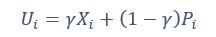
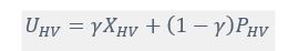
      We have provided explanations on how the reinstatement is explained by the latent cause model in the first round of the review. Briefly, both acquisition and extinction latent causes contribute to the reinstatement (test 3). The former retains the acquisition fear memory, and the latter has the updated w<sub>context</sub> from unsignaled shock. Although the reviewer is correct that the z<sub>B</sub> in Figure 1D makes a great contribution during the reinstatement, we would like to argue that the elevated CR from test 2 (trial 34) to test 3 (trial 36) is the result of the interaction between z<sub>A</sub> and z<sub>B</sub>.

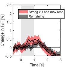
      We provided Author response image 1 using the same data in Figure 1D and 1E to further clarify this point. The posterior probability of z<sub>A</sub> increased after an unsignaled shock (trial 35), which may be attributed to the return of acquisition fear memory. The posterior probability of z<sub>A</sub> then decreased again after test 3 (trial 36) because there was no shock in this trial. Along with the weight change, the expected shock change substantially in these three trials, resulting in reinstatement. Note that the mapping of expected shock to CR in the latent cause model is controlled by parameter θ and λ. Once the expected shock exceeds the threshold θ, the CR will increase rapidly if λ is smaller.

      Lastly, accepting the idea that separate memories are responsible for acquisition and extinction in the memory modification paradigm, the latent cause model (LCM) is a rational candidate modeling this idea. Please see the following reply on why a simple model like the Rescorla-Wagner (RW) model is not sufficient to fully explain the behaviors observed in this study.

      Author response image 1.

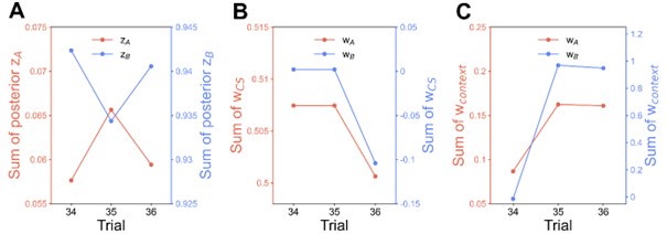
      The sum posterior probability (A), the sum of associative weight of CS (B), and the sum of associative weight of context (C) of acquisition and extinction latent causes in Figure 1D and 1E.

      (2) The authors compared the latent cause model to the Rescorla-Wagner model. This is very commendable, particularly since the latent cause model builds upon the RW model, so it can serve as an ideal test for whether a more simplified model can adequately predict the behavior. The authors show that the RW model cannot successfully predict the increased CR during reinstatement (Appendix figure 1). Yet there are some issues with the way the authors have implemented this comparison:

      (2A) The RW model is a simplified version of the latent cause model and so should be treated as a nested model when testing, or at a minimum, the number of parameters should be taken into account when comparing the models using a method such as the Bayesian Information Criterion, BIC.

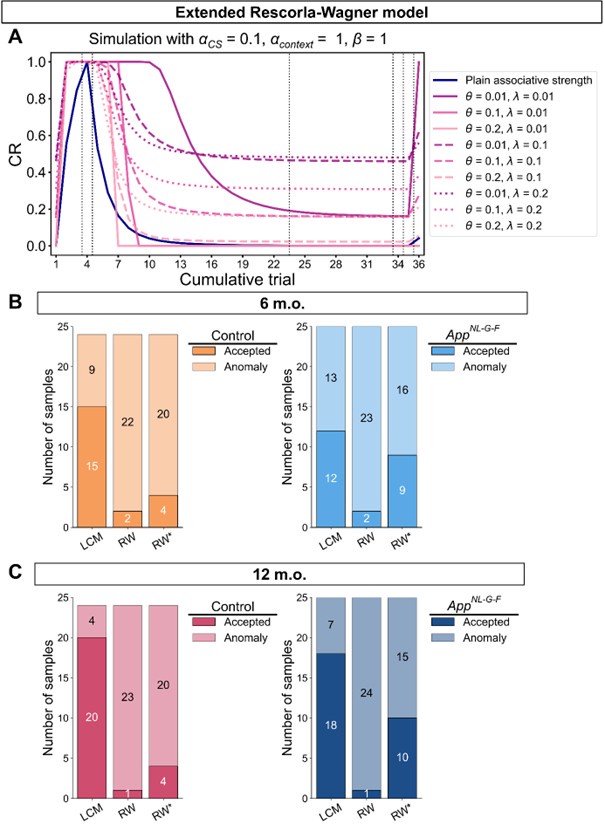
      We acknowledge that the number of parameters was not taken into consideration when we compared the models. We thank the reviewer for the suggestion to use the Bayesian Information Criterion (BIC). However, we did not use BIC in this study for the following reasons. We wanted a model that can explain fear conditioning, extinction and reinstatement, so our first priority is to fit the test phases. Models that simulate CRs well in non-test phases can yield lower BIC values even if they fail to capture reinstatement. When we calculate the BIC by using the half normal distribution (μ = 0, σ \= 0.3) as the likelihood for prediction error in each trial, the BIC of the 12-month-old control is -37.21 for the RW model (Appendix 1–figure 1C) and -11.60 for the LCM (Figure 3C). Based on this result, the RW model would be preferred, yet the LCM was penalized by the number of parameters, even though it fit better in trial 36. Because we did not think this aligned with our purpose to model reinstatement, we chose to rely on the practical criteria to determine whether the estimated parameter set is accepted or not for our purpose (see Materials and Methods). The number of accepted samples can thus roughly be seen as the model's ability to explain the data in this study. These exclusion criteria then created imbalances in accepted samples across models (Appendix 1–figure 2). In the RW model, only one or two samples met the criteria, preventing meaningful statistical comparisons of BIC within each group. Overall, though we agreed that BIC is one of the reasonable metrics in model comparison, we did not think it aligns with our purpose in this study.

      (2B) The RW model provides the associative strength between stimuli and does not necessarily require a linear relationship between V and the CR. This is the case in the original RW model as well as in the LCM. To allow for better comparison between the models, the authors should be modeling the CR in the same manner (using the same probit function) in both models. In fact, there are many instances in which a sigmoid has been applied to RW associative strengths to predict CRs. I would recommend modeling CRs in the RW as if there is just one latent cause. Or perhaps run the analysis for the LCM with just one latent cause - this would effectively reduce the LCM to RW and keep any other assumptions identical across the models.

      Regarding the suggestion to run the analysis using the LCM with one latent cause, we agree that this method is almost identical to the RW model, which is also mentioned in the original paper (Gershman et al., 2017). Importantly, it would also eliminate the RW model’s advantage of assigning distinct learning rates to different stimuli, highlighted in the next comment (2C).

      We thank the reviewer for suggesting applying the transformation of associative strength (V) to CR as in the LCM. We examined this possibility by heuristically selecting parameter values to test how such a transformation would influence the RW model (Author response image 2A). Specifically, we set α<sub>CS</sub> = 0.5, α<sub>context</sub> \= 1, β = 1, and introduced the additional parameters θ and λ, as in the LCM. This parameter set is determined heuristically to address the reviewer’s concern about a higher learning rate of context. The dark blue line is the plain associative strength. The remaining lines are CR curves under different combinations of θ and λ.

      Consistent with the reviewer’s comment, under certain parameter settings (θ \= 0.01, λ = 0.01), the extended RW model can reproduce higher CRs at test 3, thereby approximating the discrimination index observed in the 12-month-old control group. However, this modification changes the characteristics of CRs in other phases from those in the plain RW model. In the acquisition phase, the CRs rise more sharply. In the extinction phase, the CRs remain high when θ is small. Though changing λ can modulate the steepness, the CR curve is flat on the second day of the extinction phase, which does not reproduce the pattern in observed data (Figure 2B). These trade-offs suggest that the RW model with the sigmoid transformation does not improve fit quality and, in fact, sacrifices features that were well captured by simpler RW simulations (Appendix 1–figure 1A to 1D). To further evaluate this extended RW model (RW*), we applied the same parameter estimation method used in the LCM for individual data (see Materials and Methods). For each animal, α<sub>CS</sub>, α<sub>context</sub>, β, θ, and λ were estimated with their lower and upper bounds set as previously described (see Appendix 1, Materials and Methods). The results showed that the number of accepted samples slightly increased compared to the RW model without sigmoidal transformation of CR (RW* vs. RW in Author response image 2B, 2C). However, this improvement did not surpass the LCM (RW* vs. LCM in Author response image 2B, Author response image 1C). Overall, these results suggest that while using the same method to map the expected shock to CR, the RW model does not outperform the LCM. Practically, further extension, such as adding novel terms, might improve the fitting level. We would like to note that such extensions should be carefully validated if they are reasonable and necessary for an internal model, which is beyond the scope of this study. We hope this addresses the reviewer's concerns about the implementation of the RW model. 

      Author response image 2.

      Simulation (A) and parameter estimation (B and C) in the extended Rescorla-Wagner model.

      (2C) In the paper, the model fits for the alphas in the RW model are the same across the groups. Were the alphas for the two models kept as free variables? This is an important question as it gets back to the first point raised. Because the modeling of the reinstatement behavior with the LCM appears to be mainly driven by latent cause z<sub>B</sub>, the extinction memory, it may be possible to replicate the pattern of results without requiring a latent cause model. For example, the 12-month-old App NL-G-F mice behavior may have a deficit in learning about the context. Within the RW model, if the alpha for context is set to zero for those mice, but kept higher for the other groups, say alpha_context = 0.8, the authors could potentially observe the same pattern of discrimination indices in figure 2G and 2H at test. Because the authors don't explicitly state which parameters might be driving the change in the DI, the authors should show in some way that their results cannot simply be due to poor contextual learning in the 12 month old App NL-G-F mice, as this can presumably be predicted by the RW model. The authors' model fits using RW don't show this, but this is because they don't consider this possibility that the alpha for context might be disrupted in the 12-month-old App NL-G-F mice. Of course, using the RW model with these alphas won't lead to as nice of fits of the behavior across acquisition, extinction, and reinstatement as the authors' LCM, the number of parameters are substantially reduced in the RW model. Yet the important pattern of the DI would be replicated with the RW model (if I'm not mistaken), which is the important test for assessment of reinstatement.

      We would like to clarify that we estimated three parameters in the RW model for individuals:  α<sub>CS</sub>,  α<sub>context</sub>, and β. Even if we did so, many samples did not satisfy our criteria (Appendix 1–figure 2). Please refer to the “Evaluation of model fit” in Appendix 1 and the legend of Appendix 1–figure 1A to 1D, where we have written the estimated parameter values.

      We did not agree that paralyzing the contextual learning by setting  α<sub>context</sub>  as 0 in the RW model can explain the CR curve of 12-month-old AD mice well. Specifically, the RW model cannot capture the between-day extinction dynamics (i.e., the increase in CR at the beginning of day 2 extinction)  and the higher CR at test 3 relative to test 2 (i.e., DI between test 3 and test 2 is greater than 0.5). In addition, because the context input (= 0.2) was relatively lower than the CS input (= 1), and there is only a single unsignaled shock trial, even setting  α<sub>context</sub> = 1 results in only a limited increase in CR (Appendix 1–figure 1A to 1D; see also Author response image 2 9). Thus, the RW model cannot replicate the reinstatement effect or the critical pattern of discrimination index, even under conditions of stronger contextual learning.  

      (3) As stated by the authors in the introduction, the advantage of the fear learning approach is that the memory is modified across the acquisition-extinction-reinstatement phases. Although perhaps not explicitly stated by the authors, the post-reinstatement test (test 3) is the crucial test for whether there is reactivation of a previously stored memory, with the general argument being that the reinvigorated response to the CS can't simply be explained by relearning the CS-US pairing, because re-exposure the US alone leads to increase response to the CS at test. Of course there are several explanations for why this may occur, particularly when also considering the context as a stimulus. This is what I understood to be the justification for the use of a model, such as the latent cause model, that may better capture and compare these possibilities within a single framework. As such, it is critical to look at the level of responding to both the context alone and to the CS. It appears that the authors only look at the percent freezing during the CS, and it is not clear whether this is due to the contextual-US learning during the US re-exposure or to increased responding to the CS - presumably caused by reactivation of the acquisition memory. The authors do perform a comparison between the preCS and CS period, but it is not clear whether this is taken into account in the LCM. For example, the instance of the model shown in figure 1 indicates that the 'extinction cause', or cause z6, develops a strong weight for the context during the reinstatement phase of presenting the shock alone. This state then leads to increased freezing during the final CS probe test as shown in the figure. If they haven't already, I think the authors must somehow incorporate these different phases (CS vs ITI) into their model, particularly since this type of memory retrieval that depends on assessing latent states is specifically why the authors justified using the latent causal model. In more precise terms, it's not clear whether the authors incorporate a preCS/ITI period each day the cue is presented as a vector of just the context in addition to the CS period in which the vector contains both the context and the CS. Based on the description, it seemed to me that they only model the CRs during the CS period on days when the CS is presented, and thereby the context is only ever modeled on its own (as just the context by itself in the vector) on extinction days when the CS is not presented. If they are modeling both timepoints each day that the CS I presented, then I would recommend explicitly stating this in the methods section.

      In this study, we did not model the preCS freezing rate, and we thank the reviewer for the suggestion to model preCS periods as separate context-only trials. In our view, however, this approach is not consistent with the assumptions of the LCM. Our rationale is that the available periods of context and the CS are different. We assume that observation of the context lasts from preCS to CS. If we simulate both preCS (context) and CS (context and tone), the weight of context would be updated twice. Instead, we follow the same method as described in the original code from Gershman et al. (2017) to consider the context effect. We agree that explicitly modeling preCS could provide additional insights, but we believe it would require modifying or extending the LCM. We consider this an important direction for future research, but it is outside the scope of this study.

      (4) The authors fit the model using all data points across acquisition and learning. As one of the other reviewers has highlighted, it appears that there is a high chance for overfitting the data with the LCM. Of course, this would result in much better fits than models with substantially fewer free parameters, such as the RW model. As mentioned above, the authors should use a method that takes into account the number of parameters, such as the BIC.

      Please refer to the reply to public review (2A) for the reason we did not take the suggestion to use BIC. In addition, we feel that we have adequately addressed the concern of overfitting in the first round of the review. 

      (5) The authors have stated that they do not think the Barnes maze task can be modeled with the LCM. Whether or not this is the case, if the authors do not model this data with the LCM, the Barnes maze data doesn't appear valuable to the main hypothesis. The authors suggest that more sophisticated models such as the LCM may be beneficial for early detection of diseases such as Alzheimer's, so the Barnes maze data is not valuable for providing evidence of this hypothesis. Rather, the authors make an argument that the memory deficits in the Barnes maze mimic the reinstatement effects providing support that memory is disrupted similarly in these mice. Although, the authors state that the deficits in memory retrieval are similar across the two tasks, the authors are not explicit as to the precise deficits in memory retrieval in the reinstatement task - it's a combination of overgeneralizing latent causes during acquisition, poor learning rate, over differentiation of the stimuli.

      We would like to clarify that we valued the latent cause model not solely because it is more sophisticated and fits more data points, but it is an internal model that implicates the cognitive process. Please also see the reply to the recommendations to authors (3) about the reason why we did not take the suggestion to remove this data.

      Reviewer #3 (Public review):

      Summary:

      This paper seeks to identify underlying mechanisms contributing to memory deficits observed in Alzheimer's disease (AD) mouse models. By understanding these mechanisms, they hope to uncover insights into subtle cognitive changes early in AD to inform interventions for early-stage decline.

      Strengths:

      The paper provides a comprehensive exploration of memory deficits in an AD mouse model, covering early and late stages of the disease. The experimental design was robust, confirming age-dependent increases in Aβ plaque accumulation in the AD model mice and using multiple behavior tasks that collectively highlighted difficulties in maintaining multiple competing memory cues, with deficits most pronounced in older mice.

      In the fear acquisition, extinction, and reinstatement task, AD model mice exhibited a significantly higher fear response after acquisition compared to controls, as well as a greater drop in fear response during reinstatement. These findings suggest that AD mice struggle to retain the fear memory associated with the conditioned stimulus, with the group differences being more pronounced in the older mice.

      In the reversal Barnes maze task, the AD model mice displayed a tendency to explore the maze perimeter rather than the two potential target holes, indicating a failure to integrate multiple memory cues into their strategy. This contrasted with the control mice, which used the more confirmatory strategy of focusing on the two target holes. Despite this, the AD mice were quicker to reach the target hole, suggesting that their impairments were specific to memory retrieval rather than basic task performance.

      The authors strengthened their findings by analyzing their data with a leading computational model, which describes how animals balance competing memories. They found that AD mice showed somewhat of a contradiction: a tendency to both treat trials as more alike than they are (lower α) and similar stimuli as more distinct than they are (lower σx) compared to controls.

      Weaknesses:

      While conceptually solid, the model struggles to fit the data and to support the key hypothesis about AD mice's inability to retain competing memories. These issues are evident in Figure 3:

      (1) The model misses trends in the data, including the gradual learning of fear in all groups during acquisition, the absence of a fear response at the start of the experiment, and the faster return of fear during reinstatement compared to the gradual learning of fear during acquisition. It also underestimates the increase in fear at the start of day 2 of extinction, particularly in controls.

      (2) The model explains the higher fear response in controls during reinstatement largely through a stronger association to the context formed during the unsignaled shock phase, rather than to any memory of the conditioned stimulus from acquisition (as seen in Figure 3C). In the experiment, however, this memory does seem to be important for explaining the higher fear response in controls during reinstatement (as seen in Author Response Figure 3). The model does show a necessary condition for memory retrieval, which is that controls rely more on the latent causes from acquisition. But this alone is not sufficient, since the associations within that cause may have been overwritten during extinction. The Rescorla-Wagner model illustrates this point: it too uses the latent cause from acquisition (as it only ever uses a single cause across phases) but does not retain the original stimulus-shock memory, updating and overwriting it continuously. Similarly, the latent cause model may reuse a cause from acquisition without preserving its original stimulus-shock association.

      These issues lead to potential overinterpretation of the model parameters. The differences in α and σx are being used to make claims about cognitive processes (e.g., overgeneralization vs. over differentiation), but the model itself does not appear to capture these processes accurately.

      The authors could benefit from a model that better matches the data and captures the retention and retrieval of fear memories across phases. While they explored alternatives, including the Rescorla-Wagner model and a latent state model, these showed no meaningful improvement in fit. This highlights a broader issue: these models are well-motivated but may not fully capture observed behavior.

      Conclusion:

      Overall, the data support the authors' hypothesis that AD model mice struggle to retain competing memories, with the effect becoming more pronounced with age. While I believe the right computational model could highlight these differences, the current models fall short in doing so.

      We thank the reviewer for the insightful comments. For the comments (1) and (2), please refer to our previous author response to comments #26 and #27. We recognize that the models tested in this study have limitations and, as noted, do not fully capture all aspects of the observed behavioral data. We see this as an important direction for future research and value the reviewer’s suggestions.

      Recommendations for the authors:

      Reviewer #2 (Recommendations for the authors):

      I have maintained some of the main concerns included in the first round of reviews as I think they remain concerns with the new draft, even though the authors have included substantially more analysis of their data, which is appreciated. I particularly found the inclusion of the comparative modeling valuable, although I think the analysis comparing the models should be improved.

      (1) This relates to point 1 in the public assessment or #16 in the response to reviewers from the authors. The authors raise the point that even a low posterior can drive behavioral expression (lines 361-365 in the response to authors), and so the acquisition latent cause may partially drive reinstatement. Yet in the stimulation shown in figure 1D, this does not seem to be the case. As I mentioned in the public response, in figure 1, the posteriors for z<sub>A</sub> are similar on day 34 and day 36, yet only on day 36 is there a strong CR. At least in this example, it does not appear that z<sub>A</sub> contributes to the increased responding from day 34 (test 2) to day 36 (test 3). There may be a slight increase in z1 in figure 3C, but the dominant change from day 34 to day 36 appears to be the increase in the posterior of z3 and the substantial increase in w3. The authors then cite several papers which have shown the shift in balance between what it is the putative acquisition memory and extinction memory (i.e. Lacagnina et al.). Yet I do not see how this modeling fits with most of the previous findings. For example, in the Lacagnina et al. paper, activation of the acquisition ensemble or inhibition of the extinction ensemble drives freezing, whereas the opposite pattern reduces freezing. What appears to be the pattern in the modeling in this paper is primarily learning of context in the extinction latent cause to predict the shock. As I mention in point 2C of the public review, it's not clear why this pattern of results would require a latent cause model. Would a high alpha for context and not the CS not give a similar pattern of results in the RW model? At least for giving similar results of the DIs in figure 2?

      First, we would like to clarify that the x-axis in Figure 1D is labeled “Trial,” not “Day.” Please refer to the reply to public review (1), where we clarified the posterior probability of the latent cause from trials 34 to 36. Second, although we did not have direct neural circuit evidence in this study, we discussed the similarities between previous findings and the modeling in the first review. Briefly, our main point focuses on the interaction between acquisition and extinction memory. In other words, responses at different times arise from distinct internal states made up of competing memories. We assume that the reviewer expects a modeling result showing nearly full recovery of acquisition memory, which aligns with previous findings where optogenetic activation of the acquisition engram can partially mimic reinstatement (Zaki et al., 2022; see also the response to comment #12 in the first round of review). We acknowledge that such a modeling result cannot be achieved with the latent cause model and see it as a potential future direction for model improvement.

      Please also refer to the reply to public review (2) about how a high alpha for context in the RW model cannot explain the pattern we observed in the reinstatement paradigm.

      (2) This is related to point 3 in the public comments and #13 in the response to reviewers. I raised the question of comparing the preCS/ITI period with the CS period, but my main point was why not include these periods in the LCM itself as mentioned in more detail in point 3 in the current public review. The inclusion of the comparisons the authors performed helped, but my main point was that the authors could have a better measure of wcontext if they included the preCS period as a stimulus each day (when only the context is included in the stimulus). This would provide better estimates of wcontext. As stated in the public review, perhaps the authors did this, but my understanding of the methods this was not the case, rather, it seems the authors only included the CS period for CRs within the model (at least on days when the CS was present).

      Please refer to the reply to public review (3) about the reason why we did not model the preCS freezing rate.

      (3) This relates to point 4 in the public review and #15 and #24 in the response to authors. The authors have several points for why the two experiments are similar and how results may be extrapolated - lines 725-733. The first point is that associative learning is fundamental in spatial learning. I'm not sure that this broad connection between the two studies is particularly insightful for why one supports the other as associative learning is putatively involved in most behavioral tasks. In the second point about reversals, why not then use a reversal paradigm that would be easier to model with LCM? This data is certainly valuable and interesting, yet I don't think it's helpful for this paper to state qualitatively the similarities in the potential ways a latent cause framework might predict behavior on the Barnes maze. I would recommend that the authors either model the behavior with LCM, remove the experiment from the paper, or change the framing of the paper that LCM might be an ideal approach for early detection of dementia or Alzheimer's disease.

      We would like to clarify that our aim was not to present the LCM as an ideal tool for early detection of AD symptoms. Rather, our focus is on the broader idea of utilizing internal models and estimating individual internal states in early-stage AD. Regarding using a reversal paradigm that would be easier to model with LCM, the most straightforward approach is to use another type of paradigm for fear conditioning, then to examine the extent to which similar behavioral characteristics are observed between paradigms within subjects. However, re-exposing the same mice to such paradigms is constrained by strong carry-over effects, limiting the feasibility of this experiment. Other behavioral tasks relevant to AD that avoid shock generally involve action selection for subsequent observation (Webster et al., 2014), which falls outside the structure of LCM. Our rationale for including the Barnes maze task is that spatial memory deficit is implicated in the early stage of AD, making it relevant for translational research. While we acknowledge that exact modeling of Barnes maze behavior would require a more sophisticated model (as discussed in the first round of review), our intention to use the reversal Barnes maze paradigm is to suggest a presumable memory modification learning in a non-fear conditioning paradigm. We also discussed whether similar deficits in memory modification could be observed across two behavioral tasks.

      (4) Reviewer # mentioned that the change in pattern of behavior only shows up in the older mice questioning the clinical relevance of early detection. I do think this is a valid point and maybe should be addressed. There does seem to be a bit of a bump in the controls on day 23 that doesn't appear in the 6-month group. Perhaps this was initially a spontaneous recovery test indicated by the dotted vertical line? This vertical line does not appear to be defined in the figure 1 legend, nor in figures 2 and 3.

      We would like to emphasize that the App<sup>NL-G-F</sup> knock-in mouse is widely considered a model of early-stage AD, characterized by Aβ accumulation with little to no neurofibrillary tangle pathology or neuronal loss (see Introduction). By examining different ages, we can assess the contribution of both the amount and duration of Aβ accumulation as well as age-related factors. Modeling the deficit in the memory modification process in the older App<sup>NL-G-F</sup> knock-in mice, we suggested a diverged internal state in early-stage AD in older age, and this does not diminish the relevance of the model for studying early cognitive changes in AD.

      We would also like to clarify again that the x-axis in the figure is “Trial,” not “Day.” The vertical dashed lines in these figures indicate phase boundaries, and they were defined in the figure legend: in Figure 1C, “The vertical dashed lines separate the phases.”; in Figure 2B, “The dashed vertical line separates the extinction 1 and extinction 2 phases.”; in Figure 3, “The vertical dashed lines indicate the boundaries of phases.”

      (5) Are the examples in figure 3 good examples? The example for the 12-month-old control shows a substantial increase in weights for the context during test 3, but not for the CS. Yet in the bar plots in Figure 4 G and H, this pattern seems to be different. The weights for the context appear to substantially drop in the "after extinction" period as compared to the "extinction" period. It's hard to tell the change from "extinction" to "after extinction" for the CS weights (the authors change the y-axis for the CS weights but not for the context weights from panels G to H).

      We would like to clarify that in Figure 3C, the increase in weights for context is not presented during test 3 (trial 36), noted by the reviewer; rather, it is the unsignaled shock phase (trial 35).

      We assumed that the reviewer might misunderstand that the labels on the left in Figure 4, “Acquisition”, “Extinction”, and “After extinction”, indicate the time point. However, the data shown in Figure 4C to 4H are all from the same time point: test 3 (trial 36). The grouping reflects the classification of latent causes based on the trial in which they were inferred. In addition, for Figures 4G and 4H, the y‐axis limits were not set identically because the data range for “Sum of w<sub>CS</sub>” varied. This was done to ensure the visibility of all data points. In Figure 4, each dot represents one animal. Take Figure 3D as an example. The point in Figure 4G is the sum of w3 and w4 in trial 36, and the point in Figure 4H is w5 in trial 36, note that the subscript numerals indicate latent cause index. We hope this addresses the reviewer’s question about the difference between the two figures.


      The following is the authors’ response to the original reviews

      Reviewer #1 (Public review):

      Summary:

      The authors show certain memory deficits in a mouse knock-in model of Alzheimer's Disease (AD). They show that the observed memory deficits can be explained by a computational model, the latent cause model of associative memory. The memory tasks used include the fear memory task (CFC) and the 'reverse' Barnes maze. Research on AD is important given its known huge societal burden. Likewise, better characterization of the behavioral phenotypes of genetic mouse models of AD is also imperative to advance our understanding of the disease using these models. In this light, I applaud the authors' efforts.

      Strengths:

      (1) Combining computational modelling with animal behavior in genetic knock-in mouse lines is a promising approach, which will be beneficial to the field and potentially explain any discrepancies in results across studies as well as provide new predictions for future work.

      (2) The authors' usage of multiple tasks and multiple ages is also important to ensure generalization across memory tasks and 'modelling' of the progression of the disease.

      Weaknesses:

      [#1] (1) I have some concerns regarding the interpretation of the behavioral results. Since the computational model then rests on the authors' interpretation of the behavioral results, it, in turn, makes judging the model's explanatory power difficult as well. For the CFC data, why do knock-in mice have stronger memory in test 1 (Figure 2C)? Does this mean the knock-in mice have better memory at this time point? Is this explained by the latent cause model? Are there some compensatory changes in these mice leading to better memory? The authors use a discrimination index across tests to infer a deficit in re-instatement, but this indicates a relative deficit in re-instatement from memory strength in test 1. The interpretation of these differential DIs is not straightforward. This is evident when test 1 is compared with test 2, i.e., the time point after extinction, which also shows a significant difference across groups, Figure 2F, in the same direction as the re-instatement. A clarification of all these points will help strengthen the authors' case.

      We appreciate the reviewer for the critical comments. According to the latent cause framework, the strength of the memory is influenced by at least 2 parameters: associative weight between CS and US given a latent cause and posterior probability of the latent cause. The modeling results showed that a higher posterior probability of acquisition latent cause, but not higher associative weight, drove the higher test 1 CR in App<sup>NL-G-F</sup> mice (Results and Discussion; Figure 4 – figure supplement 3B, 3C). In terms of posterior, we agree that App<sup>NL-G-F</sup> mice have strong fear memory. On the other hand, this suggests that App<sup>NL-G-F</sup> mice exhibited a tendency toward overgeneralization, favoring modification of old memories, which adversely affected the ability to retain competing memories. The strong memory in test 1 would be a compensatory effect of overgeneralization.    

      To estimate the magnitude of reinstatement, at least, one would have to compare CRs between test 2 (extinction) and test 3 (reinstatement), as well as those between test 1 (acquisition) and test 3. These comparisons represent the extent to which the memory at the reinstatement is far from that in the extinction, and close to that in the acquisition. Since discrimination index (DI) has been widely used as a normalized measure to evaluate the extent to which the system can distinguish between two conditions, we applied DI consistently to behavioral and simulated data in the reinstatement experiment, and the behavioral data in the reversal Barnes maze experiment, allowing us to evaluate the discriminability of an agent in these experiments. In addition, we used DI to examine its correlation with estimated parameters, enabling us to explore how individual discriminability may relate to the internal state. We have already discussed the differences in DI between test 3 and test 1, as well as CR in test 1 between control and App<sup>NL-G-F</sup> in the manuscript and further elaborated on this point in Line 232, 745-748.   

      [#2] (2) I have some concerns regarding the interpretation of the Barnes maze data as well, where there already seems to be a deficit in the memory at probe test 1 (Figure 6C). Given that there is already a deficit in memory, would not a more parsimonious explanation of the data be that general memory function in this task is impacted in these mice, rather than the authors' preferred interpretation? How does this memory weakening fit with the CFC data showing stronger memories at test 1? While I applaud the authors for using multiple memory tasks, I am left wondering if the authors tried fitting the latent cause model to the Barnes maze data as well.

      While we agree that the deficits shown in probe test 1 may imply impaired memory function in App<sup>NL-G-F</sup> mice in this task, it would be difficult to explain this solely in terms of impairments in general memory function. The learning curve and the daily strategy changes suggested that App<sup>NL-G-F</sup> mice would have virtually intact learning ability in the initial training phase (Figure 6B, 6F, Figure 6 – figure supplement 1 and 3). For the correspondence relationship between the reinstatement and the reversal Barnes maze learning from the aspect of memory modification process, please also see our reply to comment #24. We have explained why we did not fit the latent cause model to the Barnes maze data in the provisional response.

      [#3] (3) Since the authors use the behavioral data for each animal to fit the model, it is important to validate that the fits for the control vs. experimental groups are similar to the model (i.e., no significant differences in residuals). If that is the case, one can compare the differences in model results across groups (Figures 4 and 5). Some further estimates of the performance of the model across groups would help.

      We have added the residual (i.e., observed CR minus simulated CR) in Figure 3 – figure supplement 1D and 1E. The fit was similar between control and App<sup>NL-G-F</sup> mice groups in the test trials, except test 3 in the 12-month-old group. The residual was significantly higher in the 12-month-old control mice than App<sup>NL-G-F</sup> mice, suggesting the model underestimated the reinstatement in the control, yet the DI calculated from the simulated CR replicates the behavioral data (Figure 3 – figure supplement 1A to 1C). These results suggest that the latent cause model fits our data with little systematic bias such as an overestimation of CR for the control group in the reinstatement, supporting the validity of the comparisons in estimated parameters between groups. These results and discussion have been added in the manuscript Line 269-276.

      One may notice that the latent cause model overestimated the CR in acquisition trials in all groups in Figure 3 – figure supplement 1D and 1E. We have discussed this point in the reply to comment #26, 34 questioned by reviewer 3.

      [#4] (4) Is there an alternative model the authors considered, which was outweighed in terms of prediction by this model? 

      Yes, we have further evaluated two alternative models: the Rescorla-Wagner (RW; Rescorla & Wagner, 1972) model and the latent state model (LSM; Cochran & Cisler, 2019). The RW model serves as a baseline, given its known limitations in explaining fear return after extinction. The LSM is another contemporary model that shares several concepts with the latent cause model (LCM) such as building upon the RW model, assuming a latent variable inferred by Bayes’ rule, and involving a ruminative update for memory modification. We evaluated the three models in terms of the prediction accuracy and reproducibility of key behavioral features. Please refer to the Appendix 1 for detailed methods and results for these two models.

      As expected, the RW model fit well to the data till the end of extinction but failed to reproduce reinstatement (Appendix 1 – figure 1A to 1D). Due to a large prediction error in test 3, few samples met the acceptance criteria we set (Appendix 1 – figure 2 and 3A). Conversely, the LSM reproduced reinstatement, as well as gradual learning in acquisition and extinction phases, particularly in the 12month-old control (Appendix 1 – figure 1G). The number of accepted samples in the LSM was higher than in the RW model but generally lower than in the LCM (Appendix 1 – figure 2). The sum of prediction errors over all trials in the LSM was comparable to that in the LCM in the 6-month-old group (Appendix 1 – figure 4A), it was significantly lower in the 12-month-old group (Appendix 1 – figure 4B). Especially the LSM generated smaller prediction errors during the acquisition trials than in the LCM, suggesting that the LSM might be better at explaining the behaviors of acquisition (Appendix 1 – figure 4A and 4B; but see the reply for comment #34). While the LSM generated smaller prediction errors than the LCM in test 2 of the control group, it failed to replicate the observed DIs, a critical behavioral phenotype difference between control and App<sup>NL-G-F</sup> mice (Appendix 1 – figure 6A to 6C; cf. Figure 2F to 2H, Figure 3 – figure supplement 1A to 1C).

      Thus, although each model could capture different aspects of reinstatement, standing on the LCM to explain the reinstatement better aligns with our purpose. It should also be noted that we did not explore all parameter spaces of the LSM, hence we cannot rule out the possibility that alternative parameter sets could provide a better fit and explain the memory modification process well. A more comprehensive parameter search in the LSM may be a valuable direction for future research. 

      [#5] One concern here is also parameter overfitting. Did the authors try leaving out some data (trials/mice) and predicting their responses based on the fit derived from the training data?

      Following the reviewer’s suggestion, we confirmed if overfitting occurred using all trials to estimate parameters. Estimating parameters while actually leaving out trials would disorder the time lapse across trials, and thereby the prior of latent causes in each trial. Instead, we removed the constraint of prediction error by setting the error threshold to 1 for certain trials to virtually leave these trials out. We treated these trials as a virtual “training” dataset, while the rest of the trials were a “test” dataset. For the median CR data of each group (Figure 3), we estimated parameters under 6 conditions with unique training and test trials, then evaluated the prediction error for the training and test trials. Note that training and test trials were arbitrarily decided. Also, the error threshold for the acquisition trial was set to 1 as described in Materials and Methods, which we have further discussed the reason in the reply to comment #34 and treated acquisition trials separately from the test trials. We expect that the contribution of the data from the acquisition and test trials for parameter estimation could be discounted compared to those from the training trials with the constraint, and if overfitting occurred, the prediction error in the test data would be worse than that in the training trials.

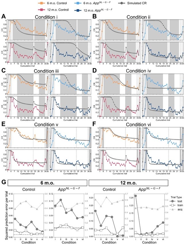
      Author response image 1A to 1F showed the simulated and observed CR under each condition, where acquisition trials were in light-shaded areas, test trials were in dark-shaded areas, and the rest of the trials were training trials. Author response image 1G showed mean squared prediction error across the acquisition, training and test trials under each condition. The dashed gray line showed the mean squared prediction error of training trials in Figure 3 as a baseline.

      In conditions i and ii, where two or four trials in the extinction were used for training (Author response image 1A and 1B), the prediction error was generally higher in test trials than in training trials. In conditions iii and iv where ten trials in the extinction were used for training (Author response image 1C and 1D), the difference in prediction error between testing and training trials became smaller. These results suggest that providing more extinction trial data would reduce overfitting. In condition v (Author response image 1E), the results showed that using trials until extinction can predict reinstatement in control mice but not App<sup>NL-G-F</sup> mice. Similarly, in condition vi (Author response image 1F), where test phase trials were left out, the prediction error differences were greater in App<sup>NL-G-F</sup> mice. These results suggest that the test trials should be used for the parameter estimation to minimize prediction error for all groups. Overall, this analysis suggests that using all trials would reduce prediction error with few overfitting. 

      Author response image 1.

      Leaving trials out in parameter estimation in the latent cause model. (A – F) The observed CR (colored line) is the median freezing rate during the CS presentation over the mice within each group, which is the same as that in Figure 3. The colors indicate different groups: orange represents 6-month-old control, light blue represents 6-month-old App<sup>NL-G-F</sup> mice, pink represents 12-month-old control, and dark blue represents 12-month-old App<sup>NL-G-F</sup> mice. Under six different leave-out conditions (i – vi), parameters were estimated and used for generating simulated CR (gray line). In each condition, trials were categorized as acquisition (light-shaded area), training data (white area), and test data (dark-shaded area) based on the error threshold during parameter estimation. Only the error threshold of the test data trial was different from the original method (see Material and Method) and set to 1. In conditions i to vi, the number of test data trials is 27, 25, 19, and 19 in extinction phases. In condition v, the number of test data trials is 2 (trials 35 and 36). In condition vi, test data trials were the 3 test phases (trials 4, 34, and 36). (G) Each subplot shows the mean squared prediction error for the test data trial (gray circles), training data trial (white squares), and acquisition trial (gray triangles) in each group. The left y-axis corresponds to data from test and training trials, and the right y-axis corresponds to data from acquisition trials. The dashed line indicates the results calculated from Figure 3 as a baseline.  

      Reviewer #1 (Recommendations for the authors):

      Minor:

      [#6] (1) I would like the authors to further clarify why 'explaining' the reinstatement deficit in the AD mouse model is important in working towards the understanding of AD i.e., which aspect of AD this could explain etc.

      In this study, we utilized the reinstatement paradigm with the latent cause model as an internal model to illustrate how estimating internal states can improve understanding of cognitive alteration associated with extensive Aβ accumulation in the brain. Our findings suggest that misclassification in the memory modification process, manifesting as overgeneralization and overdifferentiation, underlies the memory deficit in the App<sup>NL-G-F</sup> knock-in model mice. 

      The parameters in the internal model associated with AD pathology (e.g., α and σ<sub>x</sub><sup>2</sup> in this study) can be viewed as computational phenotypes, filling the explanatory gap between neurobiological abnormalities and cognitive dysfunction in AD. This would advance the understanding of cognitive symptoms in the early stages of AD beyond conventional behavioral endpoints alone.

      We further propose that altered internal states in App<sup>NL-G-F</sup> knock-in mice may underlie a wide range of memory-related symptoms in AD as we observed that App<sup>NL-G-F</sup> knock-in mice failed to retain competing memories in the reversal Barnes maze task. We speculate on how overgeneralization and overdifferentiation may explain some AD symptoms in the manuscript:

      - Line 565-569: overgeneralization may explain deficits in discriminating highly similar visual stimuli reported in early-stage AD patients as they misclassify the lure as previously learned object

      - Line 576-579: overdifferentiation may explain impaired ability to transfer previously learned association rules in early-stage AD patients as they misclassify them as separated knowledge. 

      - Line 579-582: overdifferentiation may explain delusions in AD patients as an extended latent cause model could simulate the emergence of delusional thinking

      We provide one more example here that overgeneralization may explain that early-stage AD patients are more susceptible to proactive interference than cognitively normal elders in semantic memory tests (Curiel Cid et al., 2024; Loewenstein et al., 2015, 2016; Valles-Salgado et al., 2024), as they are more likely to infer previously learned material. Lastly, we expect that explaining memory-related symptoms within a unified framework may facilitate future hypothesis generation and contribute to the development of strategies for detecting the earliest cognitive alteration in AD.  

      [#7] (2) The authors state in the abstract/introduction that such computational modelling could be most beneficial for the early detection of memory disorders. The deficits observed here are pronounced in the older animals. It will help to further clarify if these older animals model the early stages of the disease. Do the authors expect severe deficits in this mouse model at even later time points?

      The early stage of the disease is marked by abnormal biomarkers associated with Aβ accumulation and neuroinflammation, while cognitive symptoms are mild or absent. This stage can persist for several years during which the level of Aβ may reach a plateau. As the disease progresses, tau pathology and neurodegeneration emerge and drive the transition into the late stage and the onset of dementia. The App<sup>NL-G-F</sup> knock-in mice recapitulate the features present in the early stage (Saito et al., 2014), where extensive Aꞵ accumulation and neuroinflammation worsen along with ages (Figure 2 – figure supplement 1). Since App<sup>NL-G-F</sup> knock-in mice are central to Aβ pathology without tauopathy and neurodegeneration, it should be noted that it does not represent the full spectrum of the disease even at advanced ages. Therefore, older animals still model the early stages of the diseases and are suitable to study the long-term effect of Aβ accumulation and neuroinflammation. 

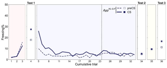
      The age tested in previous reports using App<sup>NL-G-F</sup> mice spanned a wide range from 2 months old to 24 months old. Different behavioral tasks have varied sensitivity but overall suggest the dysfunction worsens with aging (Bellio et al., 2024; Mehla et al., 2019; Sakakibara et al., 2018). We have tested the reinstatement experiment with 17-month-old App<sup>NL-G-F</sup> mice before (Author response image 2). They showed more advanced deficits with the same trends observed in 12-month-old App<sup>NL-G-F</sup> mice, but their freezing rates were overall at a lower level. There is a concern that possible hearing loss may affect the results and interpretation, therefore we decided to focus on 12-month-old data.

      Author response image 2.

      Freezing rate across reinstatement paradigm in the 17-month-old App<sup>NL-G-F</sup> mice. Dashed and solid lines indicate the median freezing rate over 34 mice before (preCS) and during (CS) tone presentation, respectively. Red, blue, and yellow backgrounds represent acquisition, extinction, and unsignaled shock in Figure 2A. The dashed vertical line separates the extinction 1 and extinction 2 phases.

      [#8] (3) There are quite a few 'marginal' p-values in the paper at p>0.05 but near it. Should we accept them all as statistically significant? The authors need to clarify if all the experimental groups are sufficiently powered.

      For our study, we decided a priori that p < 0.05 would be considered statistically significant, as described in the Materials and Methods. Therefore, in our Results, we did not consider these marginal values as statistically significant but reported the trend, as they may indicate substantive significance.

      We described our power analysis method in the manuscript Line 897-898 and have provided the results in Tables S21 and S22.

      [#9] (4) The authors emphasize here that such computational modelling enables us to study the underlying 'reasoning' of the patient (in the abstract and introduction), I do not see how this is the case. The model states that there is a latent i.e. another underlying variable that was not previously considered.

      Our use of the term “reasoning” was to distinguish the internal model, which describes how an agent makes sense of the world, from other generative models implemented for biomarker and disease progression prediction. However, we agree that using “reasoning” may be misleading and imprecise, so to reduce ambiguity we have removed this word in our manuscript Line 27: Nonetheless, internal models of the patient remain underexplored in AD; Line 85: However, previous approaches did not suppose an internal model of the world to predict future from current observation given prior knowledge.   

      [#10] (5) The authors combine knock-in mice with controls to compute correlations of parameters of the model with behavior of animals (e.g. Figure 4B and Figure 5B). They run the risk of spurious correlations due to differences across groups, which they have indeed shown to exist (Figure 4A and 5A). It would help to show within-group correlations between DI and parameter fit, at least for the control group (which has a large spread of data).

      We agree that genotype (control, App<sup>NL-G-F</sup>) could be a confounder between the estimated parameters and DI, thereby generating spurious correlations. To address this concern, we have provided withingroup correlation in Figure 4 – figure supplement 2 for the 12-month-old group and Figure 5 – figure supplement 2 for the 6-month-old group.

      In the 12-month-old group, the significant positive correlation between σx2 and DI remained in both control and App<sup>NL-G-F</sup> mice even if we adjusted the genotype effect, suggesting that it is very unlikely that the correlations in Figure 4B are due to the genotype-related confounding. On the other hand, the positive correlation between α and DI was found to be significant in the control mice but not in the App<sup>NL-G-F</sup> mice. Most of α were distributed around the lower bound in App<sup>NL-G-F</sup> mice, which possibly reduced the variance and correlation coefficient. These results support our original conclusion that α and σ<sub>x</sub><sup>2</sup> are parameters associated with a lower magnitude of reinstatement in aged App<sup>NL-G-F</sup> mice.

      In the 6-month-old group, the correlations shown in Figure 5B were not preserved within subgroups, suggesting genotype would be a confounder for α, σ<sub>x</sub><sup>2</sup>, and DI. We recognized that significant correlations in Figure 5B may arise from group differences, increased sample size, or greater variance after combining control and App<sup>NL-G-F</sup> mice. 

      Therefore, we concluded that α and σ<sub>x</sub><sup>2</sup> are associated with the magnitude of reinstatement but modulated by the genotype effect depending on the age. 

      We have added interpretations of within-group correlation in the manuscript Line 307-308, 375-378.

      [#11] (6) It is unclear to me why overgeneralization of internal states will lead to the animals having trouble recalling a memory. Would this not lead to overgeneralization of memory recall instead?

      We assume that the reviewer is referring to “overgeneralization of internal states,” a case in which the animal’s internal state remained the same regardless of the observation, thereby leading to “overgeneralization of memory recall.” We agree that this could be one possible situation and appears less problematic than the case in which this memory is no longer retrievable. 

      However, in our manuscript, we did not deal with the case of “overgeneralization of internal states”. Rather, our findings illustrated how the memory modification process falls into overgeneralization or overdifferentiation and how it adversely affects the retention of competing memories, thereby causing App<sup>NL-G-F</sup> mice to have trouble recalling the same memory as the control mice. 

      According to the latent cause model, retrieval failure is explained by a mismatch of internal states, namely when an agent perceives that the current cue does not match a previously experienced one, the old latent cause is less likely to be inferred due to its low likelihood (Gershman et al., 2017). For example, if a mouse exhibited higher CR in test 2, it would be interpreted as a successful fear memory retrieval due to overgeneralization of the fear memory. However, it reflects a failure of extinction memory retrieval due to the mismatch between the internal states at extinction and test 2. This is an example that overgeneralization of memory induces the failure of memory retrieval. 

      On the other hand, App<sup>NL-G-F</sup> mice exhibited higher CR in test 1, which is conventionally interpreted as a successful fear memory retrieval. When estimating their internal states, they would infer that their observation in test 1 well matches those under the acquisition latent causes, that is the overgeneralization of fear memory as shown by a higher posterior probability in acquisition latent causes in test 1 (Figure 4 – figure supplement 3). This is an example that over-generalization of memory does not always induce retrieval failure as we explained in the reply to comment #1. 

      Reviewer #2 (Public review):

      Summary:

      This manuscript proposes that the use of a latent cause model for the assessment of memory-based tasks may provide improved early detection of Alzheimer's Disease as well as more differentiated mapping of behavior to underlying causes. To test the validity of this model, the authors use a previously described knock-in mouse model of AD and subject the mice to several behaviors to determine whether the latent cause model may provide informative predictions regarding changes in the observed behaviors. They include a well-established fear learning paradigm in which distinct memories are believed to compete for control of behavior. More specifically, it's been observed that animals undergoing fear learning and subsequent fear extinction develop two separate memories for the acquisition phase and the extinction phase, such that the extinction does not simply 'erase' the previously acquired memory. Many models of learning require the addition of a separate context or state to be added during the extinction phase and are typically modeled by assuming the existence of a new state at the time of extinction. The Niv research group, Gershman et al. 2017, have shown that the use of a latent cause model applied to this behavior can elegantly predict the formation of latent states based on a Bayesian approach, and that these latent states can facilitate the persistence of the acquisition and extinction memory independently. The authors of this manuscript leverage this approach to test whether deficits in the production of the internal states, or the inference and learning of those states, may be disrupted in knock-in mice that show both a build-up of amyloid-beta plaques and a deterioration in memory as the mice age.

      Strengths:

      I think the authors' proposal to leverage the latent cause model and test whether it can lead to improved assessments in an animal model of AD is a promising approach for bridging the gap between clinical and basic research. The authors use a promising mouse model and apply this to a paradigm in which the behavior and neurobiology are relatively well understood - an ideal situation for assessing how a disease state may impact both the neurobiology and behavior. The latent cause model has the potential to better connect observed behavior to underlying causes and may pave a road for improved mapping of changes in behavior to neurobiological mechanisms in diseases such as AD.

      Weaknesses:

      I have several substantial concerns which I've detailed below. These include important details on how the behavior was analyzed, how the model was used to assess the behavior, and the interpretations that have been made based on the model.

      [#12] (1) There is substantial data to suggest that during fear learning in mice separate memories develop for the acquisition and extinction phases, with the acquisition memory becoming more strongly retrieved during spontaneous recovery and reinstatement. The Gershman paper, cited by the authors, shows how the latent causal model can predict this shift in latent states by allowing for the priors to decay over time, thereby increasing the posterior of the acquisition memory at the time of spontaneous recovery. In this manuscript, the authors suggest a similar mechanism of action for reinstatement, yet the model does not appear to return to the acquisition memory state after reinstatement, at least based on the examples shown in Figures 1 and 3. Rather, the model appears to mainly modify the weights in the most recent state, putatively the 'extinction state', during reinstatement. Of course, the authors must rely on how the model fits the data, but this seems problematic based on prior research indicating that reinstatement is most likely due to the reactivation of the acquisition memory. This may call into question whether the model is successfully modeling the underlying processes or states that lead to behavior and whether this is a valid approach for AD.

      We thank the reviewer for insightful comments. 

      We agree that, as demonstrated in Gershman et al. (2017), the latent cause model accounts for spontaneous recovery via the inference of new latent causes during extinction and the temporal compression property provided by the prior. Moreover, it was also demonstrated that even a relatively low posterior can drive behavioral expression if the weight in the acquisition latent cause is preserved. For example, when the interval between retrieval and extinction was long enough that acquisition latent cause was not dominant during extinction, spontaneous recovery was observed despite the posterior probability of acquisition latent cause (C1) remaining below 0.1 in Figure 11D of Gershman et al. (2017). 

      In our study, a high response in test 3 (reinstatement) is explained by both acquisition and extinction latent cause. The former preserves the associative weight of the initial fear memory, while the latter has w<sub>context</sub> learned in the unsignaled shock phase. These positive w were weighted by their posterior probability and together contributed to increased expected shock in test 3. Though the posterior probability of acquisition latent cause was lower than extinction latent cause in test 3 due to time passage, this would be a parallel instance mentioned above. To clarify their contributions to reinstatement, we have conducted additional simulations and the discussion in reply to the reviewer’s next comment (see the reply to comment #13).

      We recognize that our results might appear to deviate from the notion that reinstatement results from the strong reactivation of acquisition memory, where one would expect a high posterior probability of the acquisition latent cause. However, we would like to emphasize that the return of fear emerges from the interplay of competing memories. Previous studies have shown that contextual or cued fear reinstatement involves a neural activity switch back to fear state in the medial prefrontal cortex (mPFC), including the prelimbic cortex and infralimbic cortex, and the amygdala, including ventral intercalated amygdala neurons (ITCv), medial subdivision of central nucleus of the amygdala (CeM), and the basolateral amygdala (BLA) (Giustino et al., 2019; Hitora-Imamura et al., 2015; Zaki et al., 2022). We speculate that such transition is parallel to the internal states change in the latent cause model in terms of posterior probability and associative weight change.

      Optogenetic manipulation experiments have further revealed how fear and extinction engrams contribute to extinction retrieval and reinstatement. For instance, Gu et al. (2022) used a cued fear conditioning paradigm and found that inhibition of extinction engrams in the BLA, ventral hippocampus (vHPC), and mPFC after extinction learning artificially increased freezing to the tone cue. Similar results were observed in contextual fear conditioning, where silencing extinction engrams in the hippocampus dentate gyrus (DG) impaired extinction retrieval (Lacagnina et al., 2019). These results suggest that the weakening extinction memory can induce a return of fear response even without a reminder shock. On the other hand, Zaki et al. (2022) showed that inhibition of fear engrams in the BLA, DG, or hippocampus CA1 attenuated contextual fear reinstatement. However, they also reported that stimulation of these fear engrams was not sufficient to induce reinstatement, suggesting these fear engram only partially account for reinstatement. 

      In summary, reinstatement likely results from bidirectional changes in the fear and extinction circuits, supporting our interpretation that both acquisition and extinction latent causes contribute to the reinstatement. Although it remains unclear whether these memory engrams represent latent causes, one possible interpretation is that w<sub>context</sub> update in extinction latent causes during unsignaled shock indicates weakening of the extinction memory, while preservation of w in acquisition latent causes and their posterior probability suggests reactivation of previous fear memory. 

      [#13] (2) As stated by the authors in the introduction, the advantage of the fear learning approach is that the memory is modified across the acquisition-extinction-reinstatement phases. Although perhaps not explicitly stated by the authors, the post-reinstatement test (test 3) is the crucial test for whether there is reactivation of a previously stored memory, with the general argument being that the reinvigorated response to the CS can't simply be explained by relearning the CS-US pairing, because re-exposure the US alone leads to increase response to the CS at test. Of course there are several explanations for why this may occur, particularly when also considering the context as a stimulus. This is what I understood to be the justification for the use of a model, such as the latent cause model, that may better capture and compare these possibilities within a single framework. As such, it is critical to look at the level of responding to both the context alone and to the CS. It appears that the authors only look at the percent freezing during the CS, and it is not clear whether this is due to the contextual US learning during the US re-exposure or to increased response to the CS - presumably caused by reactivation of the acquisition memory. For example, the instance of the model shown in Figure 1 indicates that the 'extinction state', or state z6, develops a strong weight for the context during the reinstatement phase of presenting the shock alone. This state then leads to increased freezing during the final CS probe test as shown in the figure. By not comparing the difference in the evoked freezing CR at the test (ITI vs CS period), the purpose of the reinstatement test is lost in the sense of whether a previous memory was reactivated - was the response to the CS restored above and beyond the freezing to the context? I think the authors must somehow incorporate these different phases (CS vs ITI) into their model, particularly since this type of memory retrieval that depends on assessing latent states is specifically why the authors justified using the latent causal model.

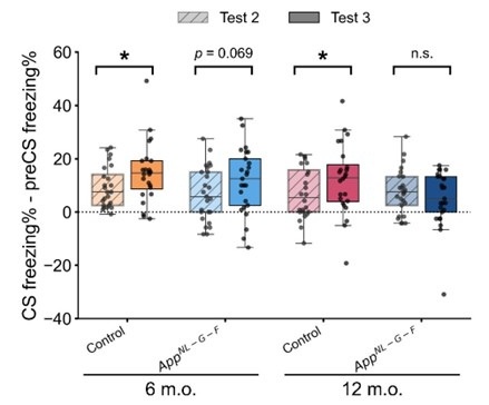
      To clarify the contribution of context, we have provided preCS freezing rate across trials in Figure 2 – figure supplement 2. As the reviewer pointed out, the preCS freezing rate did not remain at the same level across trials, especially within the 12-month-old control and App<sup>NL-G-F</sup> group (Figure 2 – figure supplement 2A and 2B), suggesting the effect context. A paired samples t-test comparing preCS freezing (Figure 2 – figure supplement 2E) and CS freezing (Figure 2E) in test 3 revealed significant differences in all groups: 6-month-old control, t(23) = -6.344, p < 0.001, d = -1.295; 6-month-old App<sup>NL-G-F</sup>, t(24) = -4.679, p < 0.001, d = -0.936; 12-month-old control, t(23) = -4.512, p < 0.001, d = 0.921; 12-month-old App<sup>NL-G-F</sup>, t(24) = -2.408, p = 0.024, d = -0.482. These results indicate that the response to CS was above and beyond the response to context only. We also compared the change in freezing rate (CS freezing rate minus preCS freezing rate) in test 2 and test 3 to examine the net response to the tone. The significant difference was found in the control group, but not in the App<sup>NL-GF</sup> group (Author response image 3). The increased net response to the tone in the control group suggested that the reinstatement was partially driven by reactivation of acquisition memory, not solely by the contextual US learning during the unsignaled shock phase. We have added these results and discussion in the manuscript Line 220-231.

      Author response image 3.

      Net freezing rate in test 2 and test 3. Net freezing rate is defined as the CS freezing rate (i.e., freezing rate during 1 min CS presentation) minus the preCS freezing rate (i.e., 1 min before CS presentation). The dashed horizontal line indicates no freezing rate change from the preCS period to the CS presentation. *p < 0.05 by paired-sample Student’s t-test, and the alternative hypothesis specifies that test 2 freezing rate change is less than test 3. Colors indicate different groups: orange represents 6-month-old control (n = 24), light blue represents 6-month-old App<sup>NL-G-F</sup> mice (n = 25), pink represents 12-month-old control (n = 24), and dark blue represents 12-month-old App<sup>NL-G-F</sup> mice (n = 25). Each black dot represents one animal. Statistical results were as follows: t(23) = -1.927, p = 0.033, Cohen’s d = -0.393 in 6-month-old control; t(24) = -1.534, p = 0.069, Cohen’s d = -0.307 in 6-month-old App<sup>NL-G-F</sup>; t(23) = -1.775, p = 0.045, Cohen’s d = -0.362 in 12-month-old control; t(24) = 0.86, p = 0.801, Cohen’s d = 0.172 in 12-monthold App<sup>NL-G-F</sup>

      According to the latent cause model, if the reinstatement is merely induced by an association between the context and the US in the unsignaled shock phase, the CR given context only and that given context and CS in test 3 should be equal. However, the simulation conducted for each mouse using their estimated parameters confirmed that this was not the case in this study. The results showed that simulated CR was significantly higher in the context+CS condition than in the context only condition (Author response image 4). This trend is consistent with the behavioral results we mentioned above.

      Author response image 4.

      Simulation of context effect in test 3. Estimated parameter sets of each sample were used to run the simulation that only context or context with CS was present in test 3 (trial 36). The data are shown as median with interquartile range, where white bars with colored lines represent CR for context only and colored bars represent CR for context with CS. Colors indicate different groups: orange represents 6-month-old control (n = 15), light blue represents 6-month-old App<sup>NL-G-F</sup> mice (n = 12), pink represents 12-month-old control (n = 20), and dark blue represents 12-month-old App<sup>NL-G-F</sup> mice (n = 18). Each black dot represents one animal. **p < 0.01, and ***p < 0.001 by Wilcoxon signed-rank test comparing context only and context + CS in each group, and the alternative hypothesis specifies that CR in context is not equal to CR in context with CS. Statistical results were as follows: W = 15, p = 0.008, effect size r = -0.66 in 6-month-old control; W = 0, p < 0.001, effect size r = -0.88 in 6-month-old App<sup>NL-G-F</sup>; W = 25, p = 0.002, effect size r = -0.67 in 12-month-old control; W = 9, p = 0.002 , effect size r = -0.75 in 12-month-old App<sup>NL-G-F</sup>

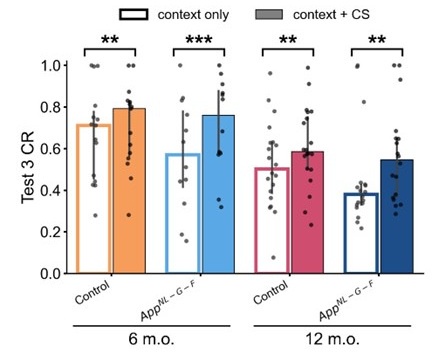
      [#14] (3) This is related to the second point above. If the question is about the memory processes underlying memory retrieval at the test following reinstatement, then I would argue that the model parameters that are not involved in testing this hypothesis be fixed prior to the test. Unlike the Gershman paper that the authors cited, the authors fit all parameters for each animal. Perhaps the authors should fit certain parameters on the acquisition and extinction phase, and then leave those parameters fixed for the reinstatement phase. To give a more concrete example, if the hypothesis is that AD mice have deficits in differentiating or retrieving latent states during reinstatement which results in the low response to the CS following reinstatement, then perhaps parameters such as the learning rate should be fixed at this point. The authors state that the 12-month-old AD mice have substantially lower learning rate measures (almost a 20-fold reduction!), which can be clearly seen in the very low weights attributed to the AD mouse in Figure 3D. Based on the example in Figure 3D, it seems that the reduced learning rate in these mice is most likely caused by the failure to respond at test. This is based on comparing the behavior in Figures 3C to 3D. The acquisition and extinction curves appear extremely similar across the two groups. It seems that this lower learning rate may indirectly be causing most of the other effects that the authors highlight, such as the low σx, and the changes to the parameters for the CR. It may even explain the extremely high K. Because the weights are so low, this would presumably lead to extremely low likelihoods in the posterior estimation, which I guess would lead to more latent states being considered as the posterior would be more influenced by the prior.

      We thank the reviewer for the suggestion about fitting and fixing certain parameters in different phases.

      However, this strategy may not be optimal for our study for the following scientific reasons.

      Our primary purpose is to explore internal states in the memory modification process that are associated with the deficit found in App<sup>NL-G-F</sup> mice in the reinstatement paradigm. We did not restrict the question to memory retrieval, nor did we have a particular hypothesis such that only a few parameters of interest account for the impaired associative learning or structure learning in App<sup>NL-G-F</sup> mice while all other parameters are comparable between groups. We are concerned that restricting questions to memory retrieval at the test is too parsimonious and might lead to misinterpretation of the results. As we explain in reply to comment #5, removing trials in extinction during parameter estimation reduces the model fit performance and runs the risk of overfitting within the individual. Therefore, we estimated all parameters for each animal, with the assumption that the estimated parameter set represents individual internal state (i.e., learning and memory characteristics) and should be fixed within the animal across all trials.  

      Figure 3 is the parameter estimation and simulation results using the median data of each group as an individual. The estimated parameter value is one of the possible cases in that group to demonstrate how a typical learning curve fits the latent cause model. The reviewer mentioned “20-fold reduction in learning rate” is the comparison of two data points, not the actual comparison between groups. The comparison between control and App<sup>NL-G-F</sup> mice in the 12-month-old group for all parameters was provided in Table S7. The Mann-Whitney U test did not reveal a significant difference in learning rate (η): 12-month-old control (Mdn = 0.09, IQR=0.23) vs. 12-month-old App<sup>NL-G-F</sup> (Mdn = 0.12, IQR=0.23), U = 199, p = 0.587.  

      We agree that lower learning rate could bias the learning toward inferring a new latent cause. However, this tendency may depend on the value of other parameters and varied in different phases in the reinstatement paradigm. Here, we used ⍺ as an example and demonstrate their interaction in Appendix 2 – table 2 with relatively extreme values: ⍺ \= {1, 3} and η \= {0.01, 0.5} while the rest of the parameters fixed at the initial guess value. 

      When ⍺ = 1, the number of latent causes across phases (K<sub>acq</sub>, K<sub>ext</sub>, K<sub>rem</sub>) remain unchanged and their posterior probability in test 3 were comparable even if η increased from 0.01 to 0.5. This is an example that lower η does not lead to inferring new latent causes because of low ⍺. The effect of low learning rate manifests in test 3 CR due to low w<sub>context, acq</sub> and w<sub>context, ext</sub>

      When ⍺ = 3, the number of acquisition latent causes (K<sub>acq</sub>) was higher in the case of η = 0.01 than that of η = 0.5, showing the effect mentioned by the reviewer. However, test 1 CR is much lower when η = 0.01, indicating unsuccessful learning even after inferring a new latent cause. This is none of the cases observed in this study. During extinction phases, the effect of η is surpassed by the effect of high ⍺, where the number of extinction latent causes (K<sub>ext</sub>) is high and not affected by η. After the extinction phases, the effect of K kicks in as the total number of latent causes reaches its value (K = 33 in this example), especially in the case of η = 0.01. A new latent cause is inferred after extinction in the condition of η = 0.5, but the CR 3 is still high as the w<sub>context, acq</sub> and w<sub>context, ext</sub> are high. This is an example that a new latent cause is inferred in spite of higher η

      Overall, the learning rate would not have a prominent effect alone throughout the reinstatement paradigm, and it has a joint effect with other parameters. Note that the example here did not cover our estimated results, as the estimated learning rate was not significantly different between control and App<sup>NL-G-F</sup> mice (see above). Please refer to the reply to comment #31 for more discussion about the interaction among parameters when the learning rate is fixed. We hope this clarifies the reviewer’s concern.

      [#15] (4) Why didn't the authors use the latent causal model on the Barnes maze task? The authors mention in the discussion that different cognitive processes may be at play across the two tasks, yet reversal tasks have been suggested to be solved using latent states to be able to flip between the two different task states. In this way, it seems very fitting to use the latent cause model. Indeed, it may even be a better way to assess changes in σx as there are presumably 12 observable stimuli/locations.

      Please refer to our provisional response about the application of the latent cause model to the reversal Barnes maze task. Briefly, it would be difficult to directly apply the latent cause model to the Barnes maze data because this task involves operant learning, and thereby almost all conditions in the latent cause model are not satisfied. Please also see our reply to comment #24 for the discussion of the link between the latent cause model and Barnes maze task. 

      Reviewer #2 (Recommendations for the authors):

      [#16] (1) I had a bit of difficulty finding all the details of the model. First, I had to mainly rely on the Gershman 2017 paper to understand the model. Even then, there were certain aspects of the model that were not clear. For instance, it's not quite clear to me when the new internal states are created and how the maximum number of states is determined. After reading the authors' methods and the Gershman paper, it seems that a new internal state is generated at each time point, aka zt, and that the prior for that state decays onwards from alpha. Yet because most 'new' internal states don't ever take on much of a portion of the posterior, most of these states can be ignored. Is that a correct understanding? To state this another way, I interpret the equation on line 129 to indicate that the prior is determined by the power law for all existing internal states and that each new state starts with a value of alpha, yet I don't see the rule for creating a new state, or for iterating k other than that k iterates at each timestep. Yet this seems to not be consistent with the fact that the max number of states K is also a parameter fit. Please clarify this, or point me to where this is better defined.

      I find this to be an important question for the current paper as it is unclear to me when the states were created. Most notably, in Figure 3, it's important to understand why there's an increase in the posterior of z<sub>5</sub> in the AD 12-month mice at test. Is state z<sub>5</sub> generated at trial 5? If so, the prior would be extremely small by trial 36, making it even more perplexing why z<sub>5</sub> has such a high posterior. If its weights are similar to z<sub>3</sub> and z<sub>4</sub>, and they have been much more active recently, why would z<sub>5</sub> come into play?

      We assume that the “new internal state" the reviewer is referring to is the “new latent cause." We would like to clarify that “internal state" in our study refers to all the latent causes at a given time point and observation. As this manuscript is submitted as a Research Advance article in eLife, we did not rephrase all the model details. Here, we explain when a new latent cause is created (i.e., the prior probability of a new latent cause is greater than 0) with the example of the 12-month-old group (Figure 3C and 3D). 

      Suppose that before the start of each trial, an agent inferred the most likely latent cause with maximum posterior, and it inferred k latent causes so far. A new latent cause can be inferred at the computation of the prior of latent causes at the beginning of each trial.  

      In the latent cause model, it follows a distance-dependent Chinese Restaurant Process (CRP; Blei and Frazier, 2011). The prior of each old latent cause is its posterior probability, which is the final count of the EM update before the current. In addition, the prior of old latent causes is sensitive to the time passage so that it exponentially decreases as a forgetting function modulated by g (see Figure 2 in Gershman et al., 2017). Simultaneously, the prior of a new cause is assigned ⍺. The new latent cause is inferred at this moment. Hence, the prior of latent causes is jointly determined by ⍺, g and its posterior probability. The maximum number of latent causes K is set a priori and does not affect the prior while k < K (see also reply to comment #30 for the discussion of boundary set for K and comment #31 for the discussion of the interaction between ⍺ and K). Note that only one new latent cause can be inferred in each trial, and (k+1)<sup>th</sup> latent cause, which has never been inferred so far, is chosen as the new latent cause.

      In our manuscript, the subscript number in zₖ denotes the order in which they were inferred, not the trial number. In Figures 3C and 3D, z<sub>3</sub> and z<sub>4</sub> were inferred in trials 5 and 6 during extinction; z<sub>5</sub> is a new latent cause inferred in trial 36. Therefore, the prior of z<sub>5</sub> is not extremely small compared to z<sub>4</sub> and z<sub>3</sub>.

      In both control and App<sup>NL-G-F</sup> mice in the 12-month-old (Figures 3C and 3D), z<sub>3</sub> is dominant until trial 35. The unsignaled shock at trial 35 generates a large prediction error as only context is presented and followed by the US. This prediction error reduces posterior of z<sub>3</sub>, while increasing the posterior of z<sub>4</sub> and w<sub>context</sub> in z<sub>3</sub> and z<sub>4</sub>. This decrease of posterior of z<sub>3</sub> is more obvious in the App<sup>NL-G-F</sup> than in the control group, prompting them to infer a new latent cause z<sub>5</sub> (Figure 3C and 3D). Although Figure 3C and 3D are illustrative examples as we explained in the reply to comment #14, this interpretation would be plausible as the App<sup>NL-G-F</sup> group inferred a significantly larger number of latent causes after the extinction with slightly higher posteriors of them than those in the control group (Figure 4E).

      [#17] (2) Related to the above, Are the states z<sub>A</sub> and z<sub>B</sub> defined by the authors to help the reader group the states into acquisition and extinction states, or are they somehow grouped by the model? If the latter is true, I don't understand how this would occur based on the model. If the former, could the authors state that these states were grouped together by the author?

      We used z<sub>A</sub> and z<sub>B</sub> annotations to assist with the explanation, so this is not grouped by the model. We have stated this in the manuscript Line 181-182.

      [#18] (3) This expands on the third point above. In Figure 3D, internal states z<sub>3</sub>, z<sub>4</sub>, and z<sub>5</sub> appear to be pretty much identical in weights in the App group. It's not clear to me why then the posterior of z<sub>5</sub> would all of a sudden jump up. If I understand correctly, the posterior is the likelihood of the observations given the internal state (presumably this should be similar across z<sub>3</sub>, z<sub>4</sub>, and z<sub>5</sub>), multiplied by the prior of the state. Z3 and Z4 are the dominant inferred states up to state 36. Why would z<sub>5</sub> become more likely if there doesn't appear to be any error? I'm inferring no error because there are little or no changes in weights on trial 36, most prominently no changes inz<sub>3</sub> which is the dominant internal state in step 36. If there's little change in weights, or no errors, shouldn't the prior dominate the calculation of the posterior which would lead to z<sub>3</sub> and z<sub>4</sub> being most prominent at trial 36?

      We have explained how z<sub>5</sub> of the 12-month-old App<sup>NL-G-F</sup> was inferred in the reply to comment #16. Here, we explain the process underlying the rapid changes of the posterior of z<sub>3</sub>, z<sub>4</sub>, and z<sub>5</sub> from trial 35 to 36.

      During the extinction, the mice inferred z<sub>3</sub> given the CS and the context in the absence of US. In trial 35, they observed the context and the unsignaled shock in the absence of the CS. This reduced the likelihood for the CS under z<sub>3</sub> and thereby the posterior of z<sub>3</sub>, while relatively increasing the posterior of z<sub>4</sub>. The associative weight between the context and the US , w<sub>context</sub>, indeed increased in both z<sub>3</sub> and z<sub>4</sub>, but w<sub>context</sub> of z<sub>4</sub> was updated more than that of z<sub>3</sub> due to its higher posterior probability. At the beginning of trial 36, a new latent cause z<sub>5</sub> was inferred with a certain prior (see also the reply for comment #16), and w<sub>5</sub> = w<sub>0</sub>, where w<sub>0</sub> is the initial value of weight. After normalizing the prior over latent causes, the emergence of z<sub>5</sub> reduced the prior probability of other latent causes compared to the case where the prior of z<sub>5</sub> is 0. Since the CS was presented while the US was absent in trial 36, the likelihood of the CS and that of the US under z<sub>3</sub>, and especially z<sub>4</sub>, given the cues and w became lower than the case in which z<sub>5</sub> has not been inferred yet. Consequently, the posterior of z<sub>5</sub> became salient (Figure 3D).

      To maintain consistency across panels, we used a uniform y-axis range. However, we acknowledge that this may make it harder to notice the changes of associative weights in Figure 3D. We have provided the subpanel in Figure 3D with a smaller y-axis limit to reveal the weight changes at trial 35 in Author response image 5.

      Author response image 5.

      Magnified view of w<sub>context</sub> and wCS in the last 3 trials in Figure 3D. The graph format is the same as in Figure 3D. The weight for CS (w<sub>CS</sub>) and that for context (w<sub>context</sub>) in each latent cause across trial 34 (test 2), 35 (unsignaled shock), and 36 (test 3) in 12-month-old App<sup>NL-G-F</sup> in Figure 3D was magnified in the upper and lower magenta box, respectively.

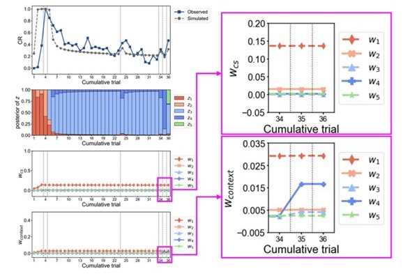
      [#19] (8) In Figure 4B - The figure legend didn't appear to indicate at which time points the DIs are plotted.

      We have amended the figure legend to indicate that DI between test 3 and test 1 is plotted.

      [#20] (9) Lines 301-303 state that the posterior probabilities of the acquisition internal states in the 12month AD mice were much higher at test 1 and that this resulted in different levels of CR across the control and 12-month App group. This is shown in the Figure 4A supplement, but this is not apparent in Figure 3 panels C and D. Is the example shown in panel D not representative of the group? The CRs across the two examples in Figure 3 C and D look extremely similar at test 1. Furthermore, the posteriors of the internal states look pretty similar across the two groups for the first 4 trials. Both the App and control have substantial posterior probabilities for the acquisition period, I don't see any additional states at test 1. The pattern of states during acquisition looks strikingly similar across the two groups, whereas the weights of the stimuli are considerably different. I think it would help the authors to use an example that better represents what the authors are referring to, or provide data to illustrate the difference. Figure 4C partly shows this, but it's not very clear how strong the posteriors are for the 3rd state in the controls.

      Figure 3 serves as an example to explain the internal states in each group (see also the third paragraph in the reply to comment #14). Figure 4C to H showed the results from each sample for between-group comparison in selected features. Therefore, the results of direct comparisons of the parameter values and internal states between genotypes in Figure 3 are not necessarily the same as those in Figure 4. Both examples in Figure 3C and 3D inferred 2 latent causes during the acquisition. In terms of posterior till test 1 (trial 4), the two could be the same. However, such examples were not rare, as the proportion of the mice that inferred 2 latent causes during the acquisition was slightly lower than 50% in the control, and around 90% in the App<sup>NL-G-F</sup> mice (Figure 4C). The posterior probability of acquisition latent cause in test 1 showed a similar pattern (Figure 4 – figure supplement 3), with values near 1 in around 50% of the control mice and around 90% of the App<sup>NL-G-F</sup> mice.  

      [#21] (10) Line 320: This is a confusing sentence. I think the authors are saying that because the App group inferred a new state during test 3, this would protect the weights of the 'extinction' state as compared to the controls since the strength of the weight updates depends on the probability of the posterior.

      In order to address this, we have revised this sentence to “Such internal states in App<sup>NL-G-F</sup> mice would diverge the associative weight update from those in the control mice after extinction.” in the manuscript Line 349-351.

      [#22] (11) In lines 517-519 the authors address the difference in generalizing the occurrence of stimuli across the App and control groups. It states that App mice with lower alpha generalized observations to an old cause rather than attributing it as a new state. Going back to statement 3 above, I think it's important to show that the model fit of a reduction in alpha does not go hand-in-hand with a reduction in the learning rates and hence the weights. Again, if the likelihoods are diminished due to the low weights, then the fit of alpha might be reduced as well. To reiterate my point above, if the observations in changes in generalization and differentiation occur because of a reduction in the learning rate, the modeling may not be providing a particularly insightful understanding of AD, other than that poor learning leads to ineffectual generalization and differentiation. Do these findings hold up if the learning rates are more comparable across the control and App group?

      These findings were explained on the basis of comparable learning rates between control and App<sup>NL-GF</sup> mice in the 12-month-old group (see the reply to comment #14). In addition, we have conducted simulation for different ⍺ and σ<sub>x</sub><sup>2</sup> values under the condition of the fixed learning rate, where overgeneralization and overdifferentaiton still occurred (see the reply to comment #26).  

      [#23] (12) Lines 391 - 393. This is a confusing sentence. "These results suggest that App NL-G-F mice could successfully form a spatial memory of the target hole, while the memory was less likely to be retrieved by a novel observation such as the absence of the escape box under the target hole at the probe test 1." The App mice show improved behavior across days of approaching the correct hole. Is this statement suggesting that once they've approached the target hole, the lack of the escape box leads to a reduction in the retention of that memory?

      We speculated that when the mice observed the absence of the escape box, a certain prediction error would be generated, which may have driven the memory modification. In App<sup>NL-G-F</sup> mice, such modification, either overgeneralization or overdifferentiation, could render the memory of the target hole vulnerable; if overgeneralization occurred, the memory would be quickly overwritten as the goal no longer exists in this position in this maze, while if overdifferentiation occurred, a novel memory such that the goal does not exist in the maze different from previous one would be formed. In either case of misclassification, the probability of retrieving the goal position would be reduced. To reduce ambiguity in this sentence, we have revised the description in the manuscript Line 432-434 as follows: “These results suggest that App<sup>NL-G-F</sup> mice could successfully form a spatial memory of the target hole, while they did not retrieve the spatial memory of the target hole as strongly as control mice when they observed the absence of the escape box during the probe test.”

      [#24] (13) The connection between the results of Barnes maze and the fear learning paradigm is weak. How can changes in overgeneralization due to a reduction in the creation of inferred states and differentiation due to a reduced σx lead to the observations in the Barnes maze experiment?

      We extrapolated our interpretation in the reinstatement modeling to behaviors in a different behavioral task, to explore the explanatory power of the latent cause framework formalizing mechanisms of associative learning and memory modification. Here, we explain the results of the reversal Barnes maze paradigm in terms of the latent cause model, while conferring the reinstatement paradigm.

      Whilst we acknowledge that fear conditioning and spatial learning are not fully comparable, the reversal Barnes maze paradigm used in our study shares several key learning components with the reinstatement paradigm. 

      First, associative learning is fundamental in spatial learning (Leising & Blaisdell, 2009; Pearce, 2009). Although we did not make any specific assumptions of what kind of associations were learned in the Barnes maze, performance improvements in learning phases likely reflect trial-and-error updates of these associations involving sensory preconditioning or secondary conditioning. Second, the reversal training phases could resemble the extinction phase in the reinstatement paradigm, challenge previously established memory. In terms of the latent cause model, both the reversal learning phase in the reversal Barnes maze paradigm and the extinction phase in the reinstatement paradigm induce a mismatch of the internal state. This process likely introduces large prediction errors, triggering memory modification to reconcile competing memories.  

      Under the latent cause framework, we posit that the mice would either infer new memories or modify existing memories for the unexpected observations in the Barnes maze (e.g., changed location or absence of escape box) as in the reinstatement paradigm, but learn a larger number of association rules between stimuli in the maze compared to those in the reinstatement. In the reversal Barnes maze paradigm, the animals would infer that a latent cause generates the stimuli in the maze at certain associative weights in each trial, and would adjust behavior by retaining competing memories.

      Both overgeneralization and overdifferentiation could explain the lower exploration time of the target hole in the App<sup>NL-G-F</sup> mice in probe test 1. In the case of overgeneralization, the mice would overwrite the existing spatial memory of the target hole with a memory that the escape box is absent. In the case of overdifferentiation, the mice would infer a new memory such that the goal does not exist in the novel field, in addition to the old memory where the goal exists in the previous field. In both cases, the App<sup>NL-G-F</sup> mice would not infer that the location of the goal is fixed at a particular point and failed to retain competing spatial memories of the goal, leading to relying on a less precise, non-spatial strategy to solve the task.  

      Since there is no established way to formalize the Barnes maze learning in the latent cause model, we did not directly apply the latent cause model to the Barnes maze data. Instead, we used the view above to explore common processes in memory modification between the reinstatement and the Barnes maze paradigm. 

      The above description was added to the manuscript on page 13 (Line 410-414) and page 19-20 (Line 600-602, 626-639).

      [#25] (14) In the fear conditioning task, it may be valuable to separate responding to the context and the cue at the time of the final test. The mice can learn about the context during the reinstatement, but there must be an inference to the cue as it's not present during the reinstatement phase. This would provide an opportunity for the model to perhaps access a prior state that was formed during acquisition. This would be more in line with the original proposal by Gershman et al. 2017 with spontaneous recovery.

      Please refer to the reply to comment #13 regarding separating the response to context in test 3.  

      Reviewer #3 (Public review):

      Summary:

      This paper seeks to identify underlying mechanisms contributing to memory deficits observed in Alzheimer's disease (AD) mouse models. By understanding these mechanisms, they hope to uncover insights into subtle cognitive changes early in AD to inform interventions for early-stage decline.

      Strengths:

      The paper provides a comprehensive exploration of memory deficits in an AD mouse model, covering the early and late stages of the disease. The experimental design was robust, confirming age-dependent increases in Aβ plaque accumulation in the AD model mice and using multiple behavior tasks that collectively highlighted difficulties in maintaining multiple competing memory cues, with deficits most pronounced in older mice.

      In the fear acquisition, extinction, and reinstatement task, AD model mice exhibited a significantly higher fear response after acquisition compared to controls, as well as a greater drop in fear response during reinstatement. These findings suggest that AD mice struggle to retain the fear memory associated with the conditioned stimulus, with the group differences being more pronounced in the older mice.

      In the reversal Barnes maze task, the AD model mice displayed a tendency to explore the maze perimeter rather than the two potential target holes, indicating a failure to integrate multiple memory cues into their strategy. This contrasted with the control mice, which used the more confirmatory strategy of focusing on the two target holes. Despite this, the AD mice were quicker to reach the target hole, suggesting that their impairments were specific to memory retrieval rather than basic task performance.

      The authors strengthened their findings by analyzing their data with a leading computational model, which describes how animals balance competing memories. They found that AD mice showed somewhat of a contradiction: a tendency to both treat trials as more alike than they are (lower α) and similar stimuli as more distinct than they are (lower σx) compared to controls.

      Weaknesses:

      While conceptually solid, the model struggles to fit the data and to support the key hypothesis about AD mice's ability to retain competing memories. These issues are evident in Figure 3:

      [#26] (1) The model misses key trends in the data, including the gradual learning of fear in all groups during acquisition, the absence of a fear response at the start of the experiment, the increase in fear at the start of day 2 of extinction (especially in controls), and the more rapid reinstatement of fear observed in older controls compared to acquisition.

      We acknowledge these limitations and explained why they arise in the latent cause model as follows.

      a. Absence of a fear response at the start of the experiment and the gradual learning of fear during acquisition 

      In the latent cause model, the CR is derived from a sigmoidal transformation from the predicted outcome with the assumption that its mapping to behavioral response may be nonlinear (see Equation 10 and section “Conditioned responding” in Gershman et al., 2017). 

      The magnitude of the unconditioned response (trial 1) is determined by w<sub>0</sub>, θ, and λ. An example was given in Appendix 2 – table 3. In general, a higher w<sub>0</sub> and a lower θ produce a higher trial 1 CR when other parameters are fixed. During the acquisition phase, once the expected shock exceeds θ, CR rapidly approaches 1, and further increases in expected shock produce few changes in CR. This rapid increase was also evident in the spontaneous recovery simulation (Figure 11) in Gershman et al. (2017). The steepness of this rapid increase is modulated by λ such that a higher value produces a shallower slope. This is a characteristic of the latent cause model, assuming CR follows a sigmoid function of expected shock, while the ordinal relationship over CRs is maintained with or without the sigmoid function, as Gershman et al. (2017) mentioned. If one assumes that the CR should be proportional to the expected shock, the model can reproduce the gradual response as a linear combination of w and posteriors of latent causes while omitting the sigmoid transformation (Figure 3). 

      b. Increase in fear at the start of day 2 extinction

      This point is partially reproduced by the latent cause model. As shown in Figure 3, trial 24 (the first trial of day 2 extinction) showed an increase in both posterior probability of latent cause retaining fear memory and the simulated CRs in all groups except the 6-month-old control group, though the increase in CR was small due to the sigmoid transformation (see above). This can be explained by the latent cause model as 24 h time lapse between extinction 1 and 2 decreases the prior of the previously inferred latent cause, leading to an increase of those of other latent causes. 

      Unlike other groups, the 6-month-old control did not exhibit increased observed CR at trial 24

      but at trial 25 (Figure 3A). The latent cause model failed to reproduce it, as there was no increase in posterior probability in trial 24 (Figure 3A). This could be partially explained by the low value of g, which counteracts the effect of the time interval between days: lower g keeps prior of the latent causes at the same level as those in the previous trial. Despite some failures in capturing this effect, our fitting policy was set to optimize prediction among the test trials given our primary purpose of explaining reinstatement.

      c. more rapid reinstatement of fear observed in older controls compared to acquisition

      We would like to point out that this was replicated by the latent cause model as shown in Figure 3 – figure supplement 1C. The DI between test 3 and test 1 calculated from the simulated CR was significantly higher in 12-month-old control than in App<sup>NL-G-F</sup> mice (cf. Figure 2C to E).  

      [#27] (2) The model attributes the higher fear response in controls during reinstatement to a stronger association with the context from the unsignaled shock phase, rather than to any memory of the conditioned stimulus from acquisition. These issues lead to potential overinterpretation of the model parameters. The differences in α and σx are being used to make claims about cognitive processes (e.g., overgeneralization vs. overdifferentiation), but the model itself does not appear to capture these processes accurately. The authors could benefit from a model that better matches the data and that can capture the retention and recollection of a fear memory across phases.

      First, we would like to clarify that the latent cause model explains the reinstatement not only by the extinction latent cause with increased w<sub>context</sub> but also the acquisition latent cause with preserved wCS and w<sub>context</sub> (see also reply to comment #13). Second, the latent cause model primarily attributes the higher fear reinstatement in control to a lower number of latent causes inferred after extinction (Figure 4E) and higher w<sub>context</sub> in extinction latent cause (Figure 4G). We noted that there was a trend toward significance in the posterior probability of latent causes inferred after extinction (Figure 4E), which in turn influences those of acquisition latent causes. Although the posterior probability of acquisition latent cause appeared trivial and no significance was detected between control and App<sup>NL-G-F</sup> mice (Figure 4C), it was suppressed by new latent causes in App<sup>NL-G-F</sup> mice (Author response image 6).

      This indicates that App<sup>NL-G-F</sup> mice retrieved acquisition memory less strongly than control mice. Therefore, we argue that the latent cause model attributed a higher fear response in control during reinstatement not solely to the stronger association with the context but also to CS fear memory from acquisition. Although we tested whether additional models fit the reinstatement data in individual mice, these models did not satisfy our fitting criteria for many mice compared to the latent cause model (see also reply to comment #4 and #28).

      Author response image 6.

      Posterior probability of acquisition, extinction, and after extinction latent causes in test 3. The values within each bar indicate the mean posterior probability of acquisition latent cause (darkest shade), extinction latent cause (medium shade), and latent causes inferred after extinction (lightest shade) in test 3 over mice within genotype. Source data are the same as those used in Figure 4C–E (posterior of z).
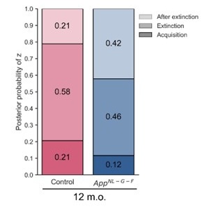
      Conclusion:

      Overall, the data support the authors' hypothesis that AD model mice struggle to retain competing memories, with the effect becoming more pronounced with age. While I believe the right computational model could highlight these differences, the current model falls short in doing so.

      Reviewer #3 (Recommendations for the authors):

      [#28] Other computational models may better capture the data. Ideally, I'd look for a model that can capture the gradual learning during acquisition, and, in some mice, the inferring of a new latent cause during extinction, allowing the fear memory to be retained and referenced at the start of day 2 extinction and during later tests.

      We have further evaluated another computational model, the latent state model, and compared it with the latent cause model. The simulation of reinstatement and parameter estimation method of the latent state model were described in the Appendix.

      The latent state model proposed by Cochran and Cisler (2019) shares several concepts with the latent cause model, and well replicates empirical data under certain conditions. We expect that it can also explain the reinstatement. 

      Following the same analysis flow for the latent cause model, we estimated the parameters and simulated reinstatement in the latent state model from individual CRs and median of them. In the median freezing rate data of the 12-month-old control mice, the simulated CR replicated the observed CR well and exhibited the ideal features that the reviewer looked for: gradual learning during acquisition and an increased fear at the start of the second-day extinction (Appendix 1 – figure 1G). However, a lot of samples did not fit well to the latent state model. The number of anomalies was generally higher than that in the latent cause model (Appendix 1 – figure 2). Within the accepted samples, the sum of squared prediction error in all trials was significantly lower in the latent state model, which resulted from lower prediction error in the acquisition trials (Appendix 1 – figure 4A and 4B). In the three test trials, the squared prediction error was comparable between the latent state model and the latent cause model except for the test 2 trials in the control group (Appendix 1 – figure 4A and 4B, rightmost panel). On the other hand, almost all accepted samples continued to infer the acquisition latent states during extinction without inferring new states (Appendix 1 – figure 5B and 5E, left panel), which differed from the ideal internal states the reviewer expected. While the latent state model fit performance seems to be better than the latent cause model, the accepted samples cannot reproduce the lower DI between test 3 and test 1 in aged App<sup>NL-G-F</sup> mice (Appendix 1 – figure 6C). These results make the latent state model less suitable for our purpose and therefore we decided to stay with the latent cause model. It should also be noted that we did not explore all parameter spaces of the latent state model hence we cannot rule out the possibility that alternative parameter sets could provide a better fit and explain the memory modification process well. A more comprehensive parameter search in the LSM may be a valuable direction for future research.

      If you decide not to go with a new model, my preference would be to drop the current modeling. However, if you wish to stay with the current model, I'd like to see justification or acknowledgment of the following:

      [#29] (1) Lower bound on alpha of 1: This forces the model to infer new latent causes, but it seems that some mice, especially younger AD mice, might rely more on classical associative learning (e.g., Rescorla-Wagner) rather than inferring new causes.

      We acknowledge that the default value set in Gershman et al. (2017) is 0.1, and the constraint we set is a much higher value. However, ⍺ = 1 does not always force the model to infer new latent causes.

      In the standard form Chinese restaurant process (CRP), the prior that n<sup>th</sup> observation is assigned to a new cluster is given by ⍺ / (n - 1 + ⍺) (Blei & Gershman, 2012). When ⍺ = 1, the prior of the new cluster for the 2nd observation will be 0.5; when ⍺ = 3, this prior increases to 0.75. Thus, when ⍺ > 1, the prior of the new cluster is above chance early in the sequence, which may relate to the reviewer’s concern. However, this effect diminishes as the number of observations increases. For instance, the prior of the new cluster drops to 0.1 and 0.25 for the 10th observation when ⍺ = 1 and 3, respectively. Furthermore, the prior in the latent cause model is governed by not only α but also g, a scaling parameter for the temporal difference between successive observations (see Results in the manuscript) following “distance-dependent” CRP, then normalized over all latent causes including a new latent cause. Thus, it does not necessarily imply that ⍺ greater than 1 forces agents to infer a new latent cause_. As shown in Appendix 2 – table 4, the number of latent causes does not inflate in each trial when _α = 1. On the other hand, the high number of latent causes due to α = 2 can be suppressed when g = 0.01. More importantly, the driving force is the prediction error generated in each trial (see also comment #31 about the interaction between ⍺ and σ<sub>x</sub><sup>2</sup>). Raising the value of ⍺ per se can be viewed as increasing the probability to infer a new latent cause, not forcing the model to do so by higher α alone. 

      During parameter exploration using the median behavioral data under a wider range of ⍺ with a lower boundary at 0.1, the estimated value eventually exceeded 1. Therefore, we set the lower bound of ⍺ to be 1 is to reduce inefficient sampling. 

      [#30] (2) Number of latent causes: Some mice infer nearly as many latent causes as trials, which seems unrealistic.

      We set the upper boundary for the maximum number of latent causes (K) to be 36 to align with the infinite features of CRP. This allowed some mice to infer more than 20 latent causes in total. When we checked the learning curves in these mice, we found that they largely fluctuated or did not show clear decreases during the extinction (Author response image 7, colored lines). The simulated learning curves were almost flat in these trials (Author response image 7, gray lines). It might be difficult to estimate the internal states of such atypical mice if the sampling process tried to fit them by increasing the number of latent causes. Nevertheless, most of the samples have a reasonable total number of latent causes: 12-month-old control mice, Mdn = 5, IQR = 4; 12-month-old App<sup>NL-G-F</sup> mice, Mdn = 5, IQR = 1.75; 6-month-old control mice, Mdn = 7, IQR = 12.5; 6-month-old App<sup>NL-G-F</sup> mice, Mdn = 5, IQR = 5.25. These data were provided in Tables S9 and S12.  

      Author response image 7.

      Samples with a high number of latent causes. Observed CR (colored line) and simulated CR (gray line) for individual samples with a total number of inferred latent causes exceeding 20. 

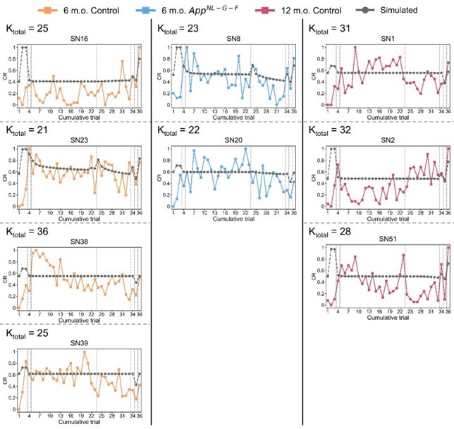
      [#31] (3) Parameter estimation: With 10 parameters fitting one-dimensional curves, many parameters (e.g., α and σx) are likely highly correlated and poorly identified. Consider presenting scatter plots of the parameters (e.g., α vs σx) in the Supplement.

      We have provided the scatter plots with a correlation matrix in Figure 4 – figure supplement 1 for the 12-month-old group and Figure 5 – figure supplement 1 for the 6-month-old group. As pointed out by the reviewer, there are significant rank correlations between parameters including ⍺ and σ<sub>x</sub><sup>2</sup> in both the 6 and 12-month-old groups. However, we also noted that there are no obvious linear relationships between the parameters.

      The correlation above raises a potential problem of non-identifiability among parameters. First, we computed the variance inflation index (VIF) for all parameters to examine the risk of multicollinearity, though we did not consider a linear regression between parameters and DI in this study. All VIF values were below the conventional threshold 10 (Appendix 2 – table 5), suggesting that severe multicollinearity is unlikely to bias our conclusions. Second, we have conducted the simulation with different combinations of ⍺, σ<sub>x</sub><sup>2</sup>, and K to clarify their contribution to overgeneralization and overdifferentiation observed in the 12-month-old group. 

      In Appendix 2 – table 6, the values of ⍺ and σ<sub>x</sub><sup>2</sup> were either their upper or lower boundary set in parameter estimation, while the value K was selected heuristically to demonstrate its effect. Given the observed positive correlation between alpha and σ<sub>x</sub><sup>2</sup>, and their negative correlation with K (Figure 4 - figure supplement 1), we consider the product of K \= {4, 35}, ⍺ \= {1, 3} and σ<sub>x</sub><sup>2</sup> \= {0.01, 3}. Among these combinations, the representative condition for the control group is α = 3, σ<sub>x</sub><sup>2</sup> = 3, and that for the App<sup>NL-G-F</sup> group is α = 1, σ<sub>x</sub><sup>2</sup> = 0.01. In the latter condition, overgeneralization and overdifferentiation, which showed higher test 1 CR, lower number of acquisition latent causes (K<sub>acq</sub>), lower test 3 CR, lower DI between test 3 and test 1, and higher number of latent causes after extinction (K<sub>rem</sub>), was extremely induced. 

      We found conditions that fall outside of empirical correlation, such as ⍺ = 3, σ<sub>x</sub><sup>2</sup> = 0.01, also reproduced overgeneralization and overdifferentiation. Similarly, the combination, ⍺ = 1, σ<sub>x</sub><sup>2</sup> = 3, exhibited control-like behavior when K = 4 but shifted toward App<sup>NL-G-F</sup>-like behavior when K = 36. The effect of K was also evident when ⍺ = 3 and σ<sub>x</sub><sup>2</sup> = 3, where K = 36 led to over-differentiation. We note that these conditions were artificially set and likely not representative of biologically plausible. These results underscore the non-identifiability concern raised by the reviewer. Therefore, we acknowledge that merely attributing overgeneralization to lower ⍺ or overdifferentiation to lower σ<sub>x</sub><sup>2</sup> may be overly reductive. Instead, these patterns likely arise from the joint effect of ⍺, σ<sub>x</sub><sup>2</sup>, and K. We have revised the manuscript accordingly in Results and Discussion (page 11-13, 18-19).

      [#32] (4) Data normalization: Normalizing the data between 0 and 1 removes the interpretability of % freezing, making mice with large changes in freezing indistinguishable seem similar to mice with small changes.

      As we describe in our reply to comment #26, the conditioned response in the latent cause model was scaled between 0 and 1, and we assume 0 and 1 mean the minimal and maximal CR within each mouse, respectively. Furthermore, although we initially tried to fit simulated CRs to raw CRs, we found that the fitting level was low due to the individual difference in the degree of behavioral expression: some mice exhibited a larger range of CR, while others showed a narrower one. Thus, we decided to normalize the data. We agree that this processing will make the mice with high changes in freezing% indistinguishable from those with low changes. However, the freezing% changes within the mouse were preserved and did not affect the discrimination index.

      [#33] (5) Overlooking parameter differences: Differences in parameters, like w<sub>0</sub>, that didn't fit the hypothesis may have been ignored.

      Our initial hypothesis is that internal states were altered in App<sup>NL-G-F</sup> mice, and we did not have a specific hypothesis on which parameter would contribute to such a state. We mainly focus on the parameters (1) that are significantly different between control and App</sup>NL-G</sup>- mice and (2) that are significantly correlated to the empirical behavioral data, DI between test 3 and test 1. 

      In the 12-month-old group, besides ⍺ and σ<sub>x</sub><sup>2</sup>, w<sub>0</sub> and K showed marginal p-value in Mann-Whitney U test (Table S7) and moderate correlation with the DI (Table S8). While differences in K were already discussed in the manuscript, we did miss the point that w<sub>0</sub> could contribute to the differences in w between control and App<sup>NL-G-F</sup> (Figure 4G) in the previous manuscript. We explain the contribution of w<sub>0</sub> on the reinstatement results here. When other parameters are fixed, higher w<sub>0</sub> would lead to higher CR in test 3, because higher w<sub>0</sub> would allow increasing w<sub>context</sub> by the unsignaled shock, leading to reinstatement (Appendix 2 – table 7). It is likely that higher w<sub>0</sub> would be sampled through the parameter estimation in the 12-month-old control but not App<sup>NL-G-F</sup>. On the other hand, the number of latent causes is not sensitive to w<sub>0</sub> when other parameters were fixed at the initial guess value (Appendix 2 – table 1), suggesting w<sub>0</sub> has a small contribution to memory modification process. 

      Thus, we speculate that although the difference in w<sub>0</sub> between control and App<sup>NL-G-F</sup> mice may arise from the sampling process, resulting in a positive correlation with DI between test 3 and test 1, its contribution to diverged internal states would be smaller relative to α or σ<sub>x</sub><sup>2</sup> as a wide range of w<sub>0</sub> has no effect on the number of latent causes (Appendix 2 – table 7). We have added the discussion of differences in w<sub>0</sub> in the 12-month-old group in manuscript Line 357-359.

      In the 6-month-old group, besides ⍺ and σ<sub>x</sub><sup>2</sup>, 𝜃 is significantly higher in the AD mice group (Table S10) but not correlated with the DI (Table S11). We have already discussed this point in the manuscript.  

      [#34] (6) Initial response: Higher initial responses in the model at the start of the experiment may reflect poor model fit.

      Please refer to our reply to comment #26 for our explanation of what contributes to high initial responses in the latent cause model.

      In addition, achieving a good fit for the acquisition CRs was not our primary purpose, as the response measured in the acquisition phase includes not only a conditioned response to the CS and context but also an unconditioned response to the novel stimuli (CS and US). This mixed response presumably increased the variance of the measured freezing rate over individuals, therefore we did not cover the results in the discussion.

      Rather, we favor models at least replicating the establishment of conditioning, extinction and reinstatement of fear memory in order to explain the memory modification process. As we mentioned in the reply for comment #4, alternative models, the latent state model and the Rescorla-Wagner model, failed to replicate the observation (cf. Figure 3 – figure supplement 1A-1C). Thus, we chose to stand on the latent cause model as it aligns better with the purpose of this study. 

      [#35] In addition, please be transparent if data is excluded, either during the fitting procedure or when performing one-way ANCOVA. Avoid discarding data when possible, but if necessary, provide clarity on the nature of excluded data (e.g., how many, why were they excluded, which group, etc?).

      We clarify the information of excluded data as follows. We had 25 mice for the 6-month-old control group, 26 mice for the 6-month-old App<sup>NL-G-F</sup> group, 29 mice for the 12-month-old control group, and 26 mice for the 12-month-old App<sup>NL-G-F</sup> group (Table S1). 

      Our first exclusion procedure was applied to the freezing rate data in the test phase. If the mouse had a freezing rate outside of the 1.5 IQR in any of the test phases, it is regarded as an outlier and removed from the analysis (see Statistical analysis in Materials and Methods). One mouse in the 6-month-old control group, one mouse in the 6-month-old App<sup>NL-G-F</sup> group, five mice in the 12-month-old control group, and two mice in the 12-month-old App<sup>NL-G-F</sup> group were excluded.

      Our second exclusion procedure was applied during the fitting and parameter estimation (see parameter estimation in Materials and Methods). We have provided the number of anomaly samples during parameter estimation in Appendix 1 – figure 2.   

      Lastly, we would like to state that all the sample sizes written in the figure legends do not include outliers detected through the exclusion procedure mentioned above.

      [#36] Finally, since several statistical tests were used and the differences are small, I suggest noting that multiple comparisons were not controlled for, so p-values should be interpreted cautiously.

      We have provided power analyses in Tables S21 and S22 with methods described in the manuscript (Line 897-898) and added a note that not all of the multiple comparisons were corrected for in the manuscript (Line 898-899).

      References cited in the response letter only 

      Bellio, T. A., Laguna-Torres, J. Y., Campion, M. S., Chou, J., Yee, S., Blusztajn, J. K., & Mellott, T. J. (2024). Perinatal choline supplementation prevents learning and memory deficits and reduces brain amyloid Aβ42 deposition in App<sup>NL-G-F</sup> Alzheimer’s disease model mice. PLOS ONE, 19(2), e0297289. https://doi.org/10.1371/journal.pone.0297289

      Blei, D. M., & Frazier, P. I. (2011). Distance Dependent Chinese Restaurant Processes. Journal of Machine Learning Research, 12(74), 2461–2488.

      Cochran, A. L., & Cisler, J. M. (2019). A flexible and generalizable model of online latent-state learning. PLOS Computational Biology, 15(9), e1007331. https://doi.org/10.1371/journal.pcbi.1007331

      Curiel Cid, R. E., Crocco, E. A., Duara, R., Vaillancourt, D., Asken, B., Armstrong, M. J., Adjouadi, M., Georgiou, M., Marsiske, M., Wang, W., Rosselli, M., Barker, W. W., Ortega, A., Hincapie, D., Gallardo, L., Alkharboush, F., DeKosky, S., Smith, G., & Loewenstein, D. A. (2024). Different aspects of failing to recover from proactive semantic interference predicts rate of progression from amnestic mild cognitive impairment to dementia. Frontiers in Aging Neuroscience, 16. https://doi.org/10.3389/fnagi.2024.1336008

      Giustino, T. F., Fitzgerald, P. J., Ressler, R. L., & Maren, S. (2019). Locus coeruleus toggles reciprocal prefrontal firing to reinstate fear. Proceedings of the National Academy of Sciences, 116(17), 8570–8575. https://doi.org/10.1073/pnas.1814278116

      Gu, X., Wu, Y.-J., Zhang, Z., Zhu, J.-J., Wu, X.-R., Wang, Q., Yi, X., Lin, Z.-J., Jiao, Z.-H., Xu, M., Jiang, Q., Li, Y., Xu, N.-J., Zhu, M. X., Wang, L.-Y., Jiang, F., Xu, T.-L., & Li, W.-G. (2022). Dynamic tripartite construct of interregional engram circuits underlies forgetting of extinction memory. Molecular Psychiatry, 27(10), 4077–4091. https://doi.org/10.1038/s41380-022-01684-7

      Lacagnina, A. F., Brockway, E. T., Crovetti, C. R., Shue, F., McCarty, M. J., Sattler, K. P., Lim, S. C., Santos, S. L., Denny, C. A., & Drew, M. R. (2019). Distinct hippocampal engrams control extinction and relapse of fear memory. Nature Neuroscience, 22(5), 753–761. https://doi.org/10.1038/s41593-019-0361-z

      Loewenstein, D. A., Curiel, R. E., Greig, M. T., Bauer, R. M., Rosado, M., Bowers, D., Wicklund, M., Crocco, E., Pontecorvo, M., Joshi, A. D., Rodriguez, R., Barker, W. W., Hidalgo, J., & Duara, R. (2016). A Novel Cognitive Stress Test for the Detection of Preclinical Alzheimer’s Disease: Discriminative Properties and Relation to Amyloid Load. The American Journal of Geriatric Psychiatry : Official Journal of the American Association for Geriatric Psychiatry, 24(10), 804–813. https://doi.org/10.1016/j.jagp.2016.02.056

      Loewenstein, D. A., Greig, M. T., Curiel, R., Rodriguez, R., Wicklund, M., Barker, W. W., Hidalgo, J., Rosado, M., & Duara, R. (2015). Proactive Semantic Interference Is Associated With Total and Regional Abnormal Amyloid Load in Non-Demented Community-Dwelling Elders: A Preliminary Study. The American Journal of Geriatric Psychiatry : Official Journal of the American Association for Geriatric Psychiatry, 23(12), 1276–1279. https://doi.org/10.1016/j.jagp.2015.07.009

      Valles-Salgado, M., Gil-Moreno, M. J., Curiel Cid, R. E., Delgado-Á lvarez, A., Ortega-Madueño, I., Delgado-Alonso, C., Palacios-Sarmiento, M., López-Carbonero, J. I., Cárdenas, M. C., MatíasGuiu, J., Díez-Cirarda, M., Loewenstein, D. A., & Matias-Guiu, J. A. (2024). Detection of cerebrospinal fluid biomarkers changes of Alzheimer’s disease using a cognitive stress test in persons with subjective cognitive decline and mild cognitive impairment. Frontiers in Psychology, 15. https://doi.org/10.3389/fpsyg.2024.1373541

      Zaki, Y., Mau, W., Cincotta, C., Monasterio, A., Odom, E., Doucette, E., Grella, S. L., Merfeld, E., Shpokayte, M., & Ramirez, S. (2022). Hippocampus and amygdala fear memory engrams reemerge after contextual fear relapse. Neuropsychopharmacology, 47(11), 1992–2001. https://doi.org/10.1038/s41386-022-01407-0

    1. Author Response

      On behalf of my co-authors, I thank you very much for sending our manuscript (# eLifeRP-RA-2023-91223) entitled “Elimination of subtelomeric repeat sequences exerts little effect on telomere functions in Saccharomyces cerevisiae” for review and providing us an opportunity for revision. We also thank the reviewers for their critical and constructive comments and suggestions which have helped us to strengthen our study. We have performed more experiments to address the concerns the reviewers raised, and we have also revised or corrected some of our statements as the reviewers suggested.

      Reviewer #1

      1) The author’s data indicate that cells with many chromosomes are more dependent on possibly homologous recombination than SY12 cells with three chromosomes. Telomerase-deficient cells exhibit the type I and type II telomere structures, whereas telomerase-deficient SY12 cells often generate different telomere structures (named Type X survivors or atypical survivors). Type I survivor depends on Rad51 possessing tandem Y' elements whereas Type II survivor depends on Rad59 carrying long TG sequences (line 60-70). Both types require Rad52 (line 66-70). At the moment, it is not determined how Type X or atypical survivors are generated in telomerase-deficient SY12 cells.

      The authors need to determine whether Type X or atypical survivors depend on other repair pathways from Type I and Type II, and what DNA sequences are retained adjacent to telomeres in Type X or atypical survivors by sequencing analysis (Fig. 2).

      We thank the reviewer’s valuable comments and suggestions. Atypical survivor is a subtype of survivor that exhibits non-uniform telomere patterns, distinct from those observed in Type I, Type II, Type X, or circular survivors. To further determine its genetic requirements, we deleted RAD52 in SY12 tlc1Δ, SY12YΔ tlc1Δ, SY12XYΔ tlc1Δ, and SY12XYΔ+Y tlc1Δ strains. Southern blotting results showed that neither Type I nor Type II survivors were found in the series of strains; circular survivor was in the predomination; beside circular survivor, some survivors exhibiting non-uniform telomere patterns suggested they were atypical survivor. These results have been presented as Figure 2—figure supplement 6B, Figure 5—figure supplement 2B and Figure 6—figure supplement 4B in the revised version. The results showed that atypical survivors still emerged when Rad52 pathway was repressed, indicating that the formation of atypical survivors does not strictly rely on the homologous recombination.

      Given that "atypical" clones exhibit non-uniform telomere patterns, it’s not surprising that their chromosome structures are variable and tanglesome. Consequently, it is hard for us to amplify and sequence the DNA sequences retained adjacent to telomeres.

      Since no Type X survivor was detected in SY12 tlc1Δ rad52Δ strain (Author response image 1A), we deleted RAD50 or RAD51 in SY12 tlc1Δ strain to investigate on which pathway the formation of the Type X survivor relied. Results showed that Type X survivor emerged in the absence of Rad51 but not Rad50, suggesting that the formation of Type X survivor depended on Rad50 pathway. These results have been presented as Figure 2—figure supplement 7.

      To determine the chromosomal end structure of the Type X survivor, we randomly selected a typical Type X survivor, and performed PCR-sequencing analysis. The results revealed the intact chromosome ends for I-L, X-R, XIII-L, XI-R, and XIV-R, albeit with some mismatches compared with the S. cerevisiae S288C genome, which possibly arising from recombination events that occurred during survivor formation. Notably, the sequence of the Y’-element in XVI-L could not be detected, while the X-element remained intact. Figure 2—figure supplement 5 in the revised manuscript.

      2) Survivor generation of each type (Type I, Type II, Type X or atypical and circularization) needs to be accurately quantitated. The authors concluded that X or Y' elements are not strictly necessary for survivor formation (Fig. 5 and Fig. 6). However, their removal appears to increase atypical survivor and chromosome circularization (Fig. 2 vs Fig. 5 and 6).

      We are grateful for the reviewer’s critical and constructive suggestions. According to the reviewer’s requirement, we quantified each type of survivors in SY12 tlc1Δ, SY12YΔ tlc1Δ, SY12XYΔ tlc1Δ and SY12XYΔ+Y tlc1Δ strains (Figure 2D, 5C, 6A and 6B). In SY12 tlc1Δ strain, Type I survivors accounted for 16%, Type II survivors for 2%, Type X survivors for 24%, circular survivors for 20% and atypical survivors for 38%. In SY12YΔ tlc1Δ strain, 4% were Type II survivors, 52% were circular survivors and 44% were atypical survivors.

      For the SY12XYΔ tlc1Δ strain, 8% were Type II survivors, 48% were circular survivors and 44% were atypical survivors. In SY12XYΔ+Y tlc1Δ strain, the proportions of Type II, circular and atypical survivors were 14%, 44%, and 42%, respectively (Author response image 1).

      In comparing SY12YΔ with SY12XYΔ, we observed a similar ratio of circular and atypical survivors. This result indicates that the remove of X-elements exert little effect on the formation of circular and atypical survivors. Similarly, in SY12XYΔ+Y strain, the proportions of circular and atypical survivors were comparable to those in SY12XYΔ strain, indicating that Y’-elements also have little effect on the formation of circular and atypical survivors. However, due to the unknown frequency of survivor formation, alternative explanations of these data are possible. For example, subtelomeric elements previously suggested to have no impact on the formation of any survivor types might influence every type to similar extents, leading to similar ratios across all survivor types. With our present data, it is still unclear whether the absence of X and Y'-elements enhances the formation of circular and atypical survivors. Therefore, we did not present these results in the revised manuscript.

      Author response image 1.

      Quantitation of each survivor type in SY12 subtelomerice engineered strains. The ratio of survivor types in SY12 tlc1Δ, SY12YΔ tlc1Δ, SY12XYΔ tlc1Δ and SY12XYΔ+Y tlc1Δ strains. Type I, pulper; Type II, green; Type X, gray; atypical survivor, orange; circular survivor, blue.

      3)The authors asked whether X and Y' elements are required for cell proliferation, stress response, telomere length control and telomere silencing (Fig. 4). Similar studies have been previously carried out by using synthetic chromosomes (see PMID: 28300123). The authors need to discuss this point.

      Thanks for your suggestion, we have added the information in the revised version. (p.24 line 449-453)

      4) The Fig. 7 data support that circular chromosomes do not require Ku-dependent DNA end protection. This is consistent with the current view that Ku binds and protects DNA ends. This finding by itself does not contribute significantly to our understanding of telomere maintenance. The authors need to more extensively discuss the significance of their findings in SY12 cells compared to wild-type cells with 16 chromosomes.

      We agree with the logic that this reviewer has pointed out. Our results demonstrate that combinatorial deletion of YKU70 and TLC1 caused synthetic lethality in SY12 cells, which possess three linear chromosomes, However, it did not affect the viability of "circular survivors", supporting the notion that telomere deprotection leads to the synthetic lethality in yku70Δ tlc1Δ double mutants. Nevertheless, this conclusion merely confirms the current view observed in wild-type cells that Ku binds and protects DNA ends.

      To avoid confusing readers and maintain the logical flow of the manuscript, we have deleted this section in the revised version.

      Minor issues:

      1) Line 112-113: " for SY13, which contains two chromosomes, could also have a high probability of circularizing all chromosomes for survival": The reference or the supplemental data are required.

      Thank this reviewer for the suggestion. According to the reviewer’s comments, we performed a Southern blotting assay to examine the types of survivors in SY13 tlc1Δ strain. We found that the majority of SY13 tlc1Δ clones exhibited hybridization signal similar to SY14 tlc1Δ circular survivors, pointing to the possibility that two chromosomes in these survivors may undergo intra-chromosomal fusions. This result has been added to figure 1D in the revised version.

      2) Line 349-350: The BY4742 mre11Δ haploid strain serves as a negative control. The authors need to explain why mre11 cells serve as a negative control.

      Thank this reviewer for the comment. We employed mre11Δ as negative control because Mre11 is a member of the RAD52 epistasis group, which is involved in the repair of double-stranded breaks in DNA, and mutants in MRE11 exhibit defects in the repair of DNA damages caused by DNA damage drugs (Krogh and Symington, 2004; Lewis et al., 2004; Symington, 2002). (p.23 line 420-422)

      Reviewer #2

      1) The qualification of survivor types mostly relies on molecular patterns in Southern blots. While this is a valid method for a standard strain, it might be more difficult to apply to the strains used in this study. For example, in SY8, SY11 and SY12, the telomere signal at 1-1.2 kb can be very faint due to the small number of terminal Y' elements left. As another example, for the Y'-less strain, it might seem obvious that no Type I survivor can emerge given that Y' amplification is a signature of Type I, but maybe Type-I-specific molecular mechanisms might still be used. To reinforce the characterization of survivor types, an analysis of the genetic requirements for Type I and Type II survivors (e.g. RAD51, RAD54, RAD59, RAD50) could complement the molecular characterization in specific result sections.

      We thank this reviewer for his/her constructive comments and suggestions. To investigate whether Type-I-specific molecular mechanisms are still utilized in the survivor formation in Y'-less strain, we deleted RAD51 in SY12XYΔ tlc1Δ. SY12XYΔ tlc1Δ rad51Δ strain was able to generate three types of survivors, including Type II survivor, circular survivor and atypical survivor, similar to the observations in SY12XYΔ tlc1Δ strain. However, the ratios of circular and atypical survivors were 36% and 32%, respectively, lower than the 48% and 44% observed in SY12XYΔ tlc1Δ strain (supplementary file 5). This result indicates that Type-I-specific molecular mechanisms contribute to the survivor formation. Given that our work primarily focuses on the function of subtelomeric elements, we chose not to include this result in our revised manuscript to maintain a coherent logical flow.

      To reinforce the characterization of survivor types, we deleted RAD50, RAD51 and RAD52 in SY12 tlc1Δ strain, respectively. Southern blotting assay revealed that in the absence of Rad51, no Type I survivor was detected; in the absence of Rad50, neither Type I nor Type X survivor was detected. However, circular and atypical survivors still emerged in the absence of Rad52, suggesting that the RAD52-mediated homologous recombination is not strictly necessary for the formation of circular and atypical survivors. These results have been presented as Figure 2—figure supplement 6 and Figure 2— figure supplement 7.

      2) In the title, the abstract and throughout the discussion, the authors chose to focus on the effect of X- and Y'-element deletion on different phenotypes and on survivor formation, as the main message to convey. While it is a legitimate and interesting message, other important results of this work might benefit from more spotlight. Namely, the observation that strains with different chromosome numbers show different survivor patterns and that several survival strategies beyond Type I and II exist and can reach substantial frequencies depending on the chromosomal context.

      Thanks for your valuable suggestion. While we value your suggestion to highlight additional aspects of our work, we would like to express our perspective on the current emphasis on the effect of X- and Y'-element deletion. We believe that by maintaining this focus, we can present a more coherent and impactful narrative for our readers. Additionally, we recognize that the relationship between chromosome numbers and survivor type frequencies is complex and warrants further experimental validation. We are considering exploring this aspect in more detail in our future projects. However, we fully acknowledge the importance of the observations you raised concerning strains with different chromosome numbers and the diversity of survival strategies.

      3) In SY12 strain, while X- and Y'-elements are not essential for survivor emergence, they do modulate the frequency of each type of survivors, with more chromosome circularization events observed for SY12YΔ, SY12XYΔ and SY12XYΔ+Y strains. This result should be stated and discussed, maybe alongside the change in survivor patterns in the other SY strains, to more accurately assess the roles of these subtelomeric elements.

      Following the reviewer’s suggestion, we compared the circular survivor ratios in SY12 tlc1Δ, SY12YΔ tlc1Δ, SY12XYΔ tlc1Δ and SY12XYΔ+Y tlc1Δ strains (supplementary file 5). It appears that the formation of circular survivors is less efficient in the SY12 tlc1Δ, with a ratio of 20%, much lower than that in SY12YΔ tlc1Δ, SY12XYΔ tlc1Δ or SY12XYΔ+Y tlc1Δ strains. However, it should be noted that SY12 tlc1Δ can generate Type I and Type X survivors, potentially decreasing the ratio of circular survivors.

      Therefore, we further compared the circular survivor ratios in SY12YΔ tlc1Δ, SY12XYΔ tlc1Δ and SY12XYΔ+Y tlc1Δ strains. In the SY12YΔ tlc1Δ strain, circular survivors accounted for 52% (26/50), comparable to 48% (24/50) in the SY12XYΔ tlc1Δ strain, indicating that X- elements exert little effect on the formation of circular survivor. Additionally, the ratio of circular survivors was 44% (22/50) in SY12XYΔ+Y tlc1Δ strain, also comparable to 48% (24/50) in the SY12XYΔ tlc1Δ strain, suggesting that Y’-element also has little effect on chromosome circularization. However, due to the unknown frequency of survivor formation, alternative explanations of these data are possible. For example, subtelomeric elements previously suggested to have no impact on the formation of any survivor types might influence every type to similar extents, resulting in similar ratios across all survivor types. With our current data, it is still uncertain whether X and Y'-elements modulate the frequency of each type of survivors. Therefore, we did not include these results in the revised manuscript.

      4) The authors might want to update some general information about subtelomere structure and their diversity across yeast strain with the recent paper by O'Donnell et al. 2023 Nature Genetics, "Telomere-to-telomere assemblies of 142 strains characterize the genome structural landscape in Saccharomyces cerevisiae".

      Thanks for your advice. We have added this information in the revised manuscript. (p.3 line 51-54)

      5) Although it is cited in the discussion, the recent work by the Malkova lab (Kockler et al. 2021 Mol Cell) could be mentioned in the introduction as it conceptually changes our views on survivor formation, its dynamics and the categorization into Type I and Type II.

      Thanks for your advice. We have added this information in the revised manuscript. (p.5 line 75-78)

      6) p.7 line 128-130: rather than chromosome number, the ratio of survivor types might be controlled by the fraction of subtelomeres with Y'-elements and their relative configuration across chromosomes. A map of the structure of remaining subtelomeres in the SYn strains might be good to have.

      We have added this information in supplementary file 2 in the revised manuscript.

      7) Fig. 1C: in SY9 tlc1Δ, the lane with triangle mark looks like a type II.

      The hybridization pattern of SY9 tlc1Δ clone 2 has both amplified Y’L-element and long heterogeneous TG1-3 repeats, it might be the “hybrid” survivor mentioned by Kockler’s work (Kockler et al., 2021). Therefore, we classify it as a no-classical survivor.

      8) p.9 line 149: the title of this result section "Y'-element is not essential for the viability of cells carrying linear chromosomes" doesn't reflect well the content of the section, which is more about characterizing the survivor pattern in SY12.

      Thanks for your advice. We have changed the title of this section into “Characterizing the survivor pattern in SY12” in the revised manuscript. (p.9 line 155)

      9) p.10 line 167: that type I can emerge in SY12 indicates that multiple Y'-elements in tandem are not required for type I recombination. I am not sure if this was already known, but it could be noted.

      We appreciate the reviewer’s comment. We have added this information in the revised manuscript. (p.10 175-177)

      10) p.18 line 318-320: the deletion of the Y' element also seems to remove the centromere-proximal telomere sequence adjacent to it. Maybe it should be stated as well. Even more importantly, in lines 327-329, the Y'-element that is reintroduced in the strain does not include the centromere-proximal short telomere sequence. This is important to interpret the Southern blots.

      We thank the reviewer for this critical suggestion. The deletion of Y'-element including both Y’- and X- element sequence in XVI-L (supplementary file 4), and the Y’element in the XVI-L does not contain the centromere-proximal telomere sequence. The Y'-element reintroduced into the left arm of Chr 3 in SY12XYΔ strain was cloned from native left arm of XVI in SY12 strain which does not contain the centromere-proximal short telomere sequence. Besides listing these details in supplementary file 4, we also emphasize it in the revised manuscript (p.21 line 397-398).

      11) p.29 lines 496-497: it seems that X and Y'-elements tend to inhibit formation of circular survivors either directly (by participating in end protection), or by promoting type I and type II, thus reducing the fraction of circular survivors. Maybe this could be added to the conclusion of this section.

      We thank the reviewer for his/her comments and have analyzed survivor types in SY12 tlc1Δ, SY12YΔ tlc1Δ, SY12XYΔ tlc1Δ and SY12XYΔ+Y tlc1Δ strains (supplementary file 5). Circular survivor formation appears less efficient in the SY12 tlc1Δ, with a ratio of 20%, significantly lower than SY12YΔ tlc1Δ, SY12XYΔ tlc1Δ or SY12XYΔ+Y tlc1Δ strains. However, it is noteworthy that SY12 tlc1Δ can generate Type I and Type X survivors, potentially impacting the circular survivor ratio.

      We further compared circular survivor ratios in SY12YΔ tlc1Δ, SY12XYΔ tlc1Δ and SY12XYΔ+Y tlc1Δ strains. SY12YΔ tlc1Δ had 52% circular survivors, similar to SY12XYΔ tlc1Δ with 48%, indicating minimal impact of X- elements. Additionally, SY12XYΔ+Y tlc1Δ had 44% circular survivors, also similar to SY12XYΔ tlc1Δ, suggesting that Y’-element has little effect on chromosome circularization. However, due to unknown frequency of survivor formation, alternative explanations, like subtelomeric elements affecting all the type of survivor similarly, are possible. With our current data, it remains unclear whether X and Y'-elements are involved in end protection and consequently inhibit the formation of circular survivors.

      Therefore, these results were not included in the revised manuscript.

      12) p.32 line 533: this result section doesn't really fit with the rest of the paper, does it?

      Thanks for your valuable advice. To avoid confusing readers and to keep the fluency of logic flow of the manuscript we have deleted this section in the revised version.

      13) The methods section does not describe the experiments sufficiently and it often lacks specific details such as the manufacturer or references. Some sections of the methods are more exhaustive than others. They should all be written with the same level of detail in my opinion.

      Thanks for your advice. We have described the experiments more sufficiently and added the manufacturer or references in the ‘materials and methods’ part in the revised manuscript. (p.41 line741-745, p.42 line 755-756, p.42 line 762-770, p.43 line 788 and p.45 line 812-813)

      Minor comments, typos and grammatical errors:

      p.3 line 33: "INTROUDUCTION" should be "INTRODUCTION".

      We have corrected it in the revised manuscript. (p.3 line 33) p.4 line 54: "S, cerevisiae", use dot instead of comma. R15: We have corrected it in the revised manuscript. (p.4 line 57)

      p.4 line 55: I believe TLC1 as the RNA moiety should be in (non-italicized) capital letters and not written as a protein.

      We have corrected it in the revised manuscript. (p.4 line 58)

      p.7 line 115: please indicate that pRS316 uses URA3 as a marker, otherwise the counterselection with 5'-FOA is not obvious.

      Thank this reviewer for the comment. We have added this statement in the revised manuscript. (p.7 line 121-122)

      p.12 line 206: tlc1Δ should be in italic.

      We have corrected it in the revised manuscript. (p.10 line 184)

      p.13 lines 227-229: "where only one hybridization signal", a verb seems to be missing.

      We thank the reviewer’s kind reminder and have corrected the mentioned errors in the revised manuscript. (p.14 line 254-255)

      Reviewer #3

      1) A weakness of the manuscript is the analysis of telomere transcriptional silencing. They state: "The results demonstrated a significant increase in the expression of the MPH3 and HSP32 upon Sir2 deletion, indicating that telomere silencing remains effective in the absence of X and Y'-elements". However, there are no statistical analyses performed as far as I can see. For some of the strains, the significance of the increased expression in sir2 (especially for MPH3) looks questionable. In addition, a striking observation is that the SY12 strain (with only three chromosomes) express much less of both MPH3 and HSP32 than the parental strain BY4742 (16 chromosomes), both in the presence and absence of Sir2. In fact, the expression of both MPH3 and HSP32 in the SY12 sir2 strain is lower than in the BY4742 SIR2+ strain. In addition, relating this work to previous studies of subtelomeric sequences in other organisms would make the discussion more interesting.

      First, I enjoyed reading your manuscript. It would be great if you performed the statistical analysis on the RT-qPCR data in figure 4B and addressed the issue of the difference of the BY4742 and SY12 strains. A model could be that this is a titration effect of silencing proteins due to fewer telomeres, which could be investigated by performing the analyses on more SY-strains with variable numbers of telomeres.

      We highly appreciate the reviewer’s valuable comments and suggestions, which included a point that has also left us confused. We conducted statistical analyses on the RT-qPCR data, and the t-test result revealed that upon the deletion of Sir2, SY12YΔ, SY12XYΔ and SY12XYΔ+Y strains exhibited a significant increase in MPH3 expression (located on the right arm of chr X) with a P value < 0.05. In the case of SY12, the deletion of Sir2 resulted in an increase in gene expression (P value < 0.1). Similar tendencies were observed in the BY4742 strain. The statistical analyses of RTqPCR results on XVI-L mirrored those of X-R.

      The results demonstrated a significant increase in MPH3 and HSP32 expression upon SIR2 deletion in SY12YΔ, SY12XYΔ and SY12XYΔ+Y strains, leading to the conclusion that telomere silencing remains effective in the absence of X-and Y’-elements. However, as the reviewer has pointed out, no statistically significant differences in MPH3 and HSP32 expression were observed between the SY12 and SY12 sir2Δ strain. For HSP32, this lack of significance may be attributed to the greater distance between HSP32 and telomere XVI-L in SY12 compared to SY12YΔ, SY12XYΔ or SY12XYΔ+Y strains, resulting in a weaker telomere position effect on HSP32 and a non-significant increase in gene expression in SY12. However, this explanation does not apply to MPH3, as SY12YΔ, with a same distance between MPH3 and telomere X-R as in SY12, still exhibits an effective telomere position effect on MPH3. We cannot provide a compelling explanation at this moment, and we suspect that the lack of statistically significant differences may be due to random clonal variation.

      Additionally, the SY12 strain (with three chromosomes) exhibited lower expression levels of both MPH3 and HSP32 compared to the parental strain BY4742 (with 16 chromosomes). Notably, it has been reported that the expression of genes coding silencing proteins in SY14 (with one chromosomes) were nearly identical to that of BY4742 (with 16 chromosomes)(Shao et al., 2018). Consequently, with respect to the reduced chromosome numbers, the silencing proteins appeared to be relatively overexpressed. Therefore, as pointed out by the reviewer, this observed phenomenon may be attributed to a titration effect of silencing proteins due to fewer telomeres. We have added the statistical analyses result in Figure 4B.

      We have related our work with previous studies of subtelomeric sequences in fission yeast in the discussion part. (p.37 line 655-676)

      Minor points are to correct the figure legend for Figure 6 supplement 1 (the strain designations) and line 55, RNAs are written with all caps, i.e. TLC1, and line 537 delete the "which" in the sentence.

      Thanks for your advice. We have corrected them in the revised manuscript.

      1) The strain has been replaced with SY12XYΔ+Y (p.35 line 617, 618 and 620)

      2) “Tlc1” has been replaced with “TLC1” (p.4 line 58).

      3) We have deleted the section of “Circular chromosome maintain stable when double knockout of yku70 and tlc1” according to the suggestions raised by reviewer 1 and 2, the deleted section contain the sentence in line 537 you mentioned.

      Kockler, Z.W., Comeron, J.M., and Malkova, A. (2021). A unified alternative telomerelengthening pathway in yeast survivor cells. Molecular Cell 81, 1816-1829.e1815. Krogh, B.O., and Symington, L.S. (2004). Recombination proteins in yeast. Annu Rev Genet 38, 233-271.

      Lewis, L.K., Storici, F., Van Komen, S., Calero, S., Sung, P., and Resnick, M.A. (2004). Role of the nuclease activity of Saccharomyces cerevisiae Mre11 in repair of DNA double-strand breaks in mitotic cells. Genetics 166, 1701-1713.

      Shao, Y., Lu, N., Wu, Z., Cai, C., Wang, S., Zhang, L.L., Zhou, F., Xiao, S., Liu, L., Zeng, X., et al. (2018). Creating a functional single-chromosome yeast. Nature 560, 331-335. Symington, L.S. (2002). Role of RAD52 epistasis group genes in homologous recombination and double-strand break repair. Microbiol Mol Biol Rev 66, 630-670, table of contents.

    1. Author response:

      The following is the authors’ response to the original reviews

      Reviewer #1:

      The chosen classification scheme for aGPCRs may require reassessment and amendment by the authors in order to prevent confusion with previously issued classification attempts of this family. (…) Can the authors suggest another scheme (mind to avoid the subfamily IIX or the alternative ADGRA-G,L,V subfamily schemes of metazoan aGPCRs), and adapt their numbering throughout the text and all figures/supplementary figures/supplementary files?

      We appreciate the reviewer's comment and agree that a different nomenclature should be used for choanoflagellate aGPCRs to avoid possible confusion. We have now re-labeled the choanoflagellate aGPCR subfamilies, previously numbered from I to XIX, using alphabetical enumeration (from A to S). Changes have been made throughout the main text, in Figure 5, and in Supplementary Figures S6 and S7.

      line 10: The abbreviation 'GPCR-TKL/Ks' is not explained.

      Thank you for pointing this out. We have now revised the text to explain the abbreviation:

      “Adhesion GPCRs and a class of GPCRs fused to kinases (the GPCR-TKL/Ks) are the most abundant GPCRs in choanoflagellates.”

      line 30: "7TM domain is diagnostic for GPCRs": strange wording. Use an alternative expression.

      We changed the wording to: 

      “A conserved seven transmembrane (7TM) domain is a hallmark of GPCRs, while the wide spectrum of extracellular and intracellular domains in some GPCRs reflects the diversification of the gene family and its functions (Schiöth and Lagerström 2008).”

      line 33: In the case of rhodopsins, not the GPCR (i.e., the apoprotein) responds directly to photons, but the retinal, which isomerises upon illumination.

      We thank the reviewer for bringing this to our attention, and we have now removed mention of photons from the list of cues detected by GPCRs.

      “For example, the extracellular N-terminus and the three extracellular loops of the 7TM domain respond to a wide range of cues, including odorant molecules, peptides, amines, lipids, nucleotides, and other molecules (Yang et al. 2021).”

      line 111: What are "genome-enabled choanoflagellates"? Explain the term. As it stands, it doesn't make sense to me.

      We meant only to highlight that these two species have sequenced genomes. We have deleted the phrase “genome enabled.”

      “To assess the predictive power of our protein-detection pipeline, we then compared the new GPCR and cytosolic signaling component datasets from two choanoflagellates – Salpingoeca rosetta and Monosiga brevicollis – with previously published GPCR and downstream GPCR signaling component counts for these two species (Nordström et al. 2009a; Krishnan et al. 2012; De Mendoza et al. 2014; Krishnan et al. 2015; Lokits et al. 2018).”

      line 145: Please give a reasoning for the naming of each of the new families (e.g., RemiSens, Hidden Gold, GPCR-TLK/K, etc.) or at least the explanations of the acronyms/names early in the manuscript, even if they are discussed later in more detail.

      Thank you for identifying this as an area of confusion. While we feel that going into the rationale behind each of the names here would interrupt the flow of the manuscript, we have added a phrase encouraging readers to “hold that thought” with the hope that they can wait for the sections that specifically focus on each of these new GPCR families.

      “This left twelve new GPCR families that had not, to our knowledge, been previously detected in choanoflagellates: Rhodopsin, TMEM145, GPR180, TMEM87, GPR155, GPR157, and six additional GPCR families that appear to fall outside all previously characterized GPCR families in eukaryotes. For reasons that will be discussed further below, we have named these six new GPCR families “Rémi-Sans-Famille” (RSF), “Hidden Gold” (Hi-GOLD), GPCR-TKL/K, GPRch1, GPRch2, and GPRch3. (Fig. 1B; Table 1).”

      lines 297/298 and 2049: Rename tethered agonist "peptide" to "element". Synthetic peptides resembling the TA were used in experiments to test for the sufficiency of the TA for receptor activation, but because the naturally occurring TAs are part of the receptor protein, they are not peptides.

      Thank you for pointing this out. We have revised the text as suggested.

      line 2026: I think the letters in the acronym "CMR" are mixed up and were intended to read "CRM".

      Good catch! We have corrected the text.

      line 2048: "diagnostic" again. Change to "tell-tale", "hallmark", or another similar descriptor.

      We have corrected the text accordingly.

      2058: Strike "motif" in order to avoid confusion with the now obsolete term "GPS motif", which entailed the five most C-terminal β-strands of GAIN subdomain B (not thus neither the full GAIN domain nor the GPS).

      Thank you for pointing this out. We have corrected the text.

      Figure 5: Did the authors also find homologs placed in the aGPCR family based on their 7TM domain sequence but lacking a GAIN domain similar to vertebrate ADGRA/GPR123, the only aGPCR known to lack a GAIN domain (10.1016/j.tips.2013.06.002)? Irrespective of the authors' findings or non-finding on that matter, please insert a note on this in the results text.

      We thank the reviewer for bringing this interesting point to our attention. We have now added a new supplementary figure A in Fig. S9 to answer the reviewer's comment. We also modified the legend of Fig. S9  to take into account this change and uploaded a new supplementary data file 20 to support Fig. S9A. Finally, we revised the main text under the section “Adhesion GPCRs” as requested: 

      Lines 328-331: “ While the GAIN and aGPCR 7TM domains evolved before the origin of opisthokonts (Araç et al.2012; Krishnan et al. 2012; De Mendoza et al. 2014), we detected the fusion of these two domains into a single module (GAIN/7TM) in most, but not all, holozoan aGPCRs (Fig. 5D, Fig.S7B and S9A; Supplementary file 20; Prömel et al, 2013; Krishnan et al. 2014).

      Reviewer #2:

      While the study contributes several interesting observations, it does not radically revise the evolutionary history of the GPCR family. However, in an era increasingly concerned with the reproducibility of scientific findings, this is arguably a strength rather than a weakness. It is encouraging to see that previously established patterns largely hold, and that with expanded sampling and improved methods, new insights can be gained, especially at the level of specific GPCR subfamilies. Then, no functional follow-ups are provided in the model system Salpingoeca rosetta, but I am sure functional work on GPCRs in choanoflagellates is set to reveal very interesting molecular adaptations in the future.

      We agree with the reviewer and anticipate that this work will provide a useful resource to motivate the future functional characterization of GPCRs in choanoflagellates, other CRMs, as well as in metazoans.

      The GPCR-TKL fusion is a particularly interesting finding, especially given the presence of such sequences in sponges. This could potentially represent a synapomorphy shared between sponges and choanoflagellates, later lost in other animals. The authors mention that BLASTP searches using the kinase domain recover the sponge GPCR-TKLs, suggesting the fusion may be ancestral. It would be useful to include phylogenetic trees of both the GPCR and TKL domains to assess this possibility. The authors might also consider examining sponge genomes released by the DTOL project to increase representation from this group.

      We agree and thank the reviewer for this suggestion. We have now added the requested phylogenetic analyses to the new Figure S17, revised the supplementary files and Methods accordingly, and commented on these results in the main text under the section “GPCR-TKL/K and GPCR-TKs“.  

      Lines 579 – 589: “While no metazoan homologs were found when using the 7TM domain of choanoflagellate GPCR-TKs as queries, using the conserved tyrosine kinase domains as queries recovered GPCR-TKs in sponges but not in other metazoan lineages or other holozoans (Fig. S17E). To test whether GPCR-TKs in sponges and choanoflagellates are homologous, we performed phylogenetic analyses of their TK and 7TM domains (Fig. S17F and G). While the TK domains of GPCR-TKs from sponges and choanoflagellates formed a well-supported clade, their 7TM domains did not. These results point to a heterogeneous evolutionary history that may include domain swapping (i.e. ancestral GPCR-TKs in which the 7TM domain was replaced in either the sponge or choanoflagellate lineages) or convergent evolution, in which homologous 7TM domains fused with unrelated 7TM domains in the sponge and choanoflagellate lineages.”

      Added to the Method section “Sequence alignment and phylogenetic analyses”:

      Lines 913 – 933: “Phylogenetic analyses of holozoan aGPCRs, Glutamate Receptors, and Gα subunits, and the 7TM and Kinase domains from GPCR TK/TKL/Ks were performed in this study. (…) To construct the phylogenies of the Kinase domain and 7TM domain from the GPCR TK/TKL/Ks, we first built a dataset including all the GPCR TK/TKL/Ks sequences identified in choanoflagellates and in sponges, as well as the GPCR TKL/Ks previously published in oomycetes and amoebozoans (Van Den Hoogen et al. 2018). We extracted the 7TM domain and Kinase domain from each sequence by combining the transmembrane domain prediction tool TMHMM-2.0 and the protein domain prediction tool InterProScan with the alignment tool MAFFT (E-INS-I algorithm) on Geneious Prime v2024.07 (Supplementary Files 30 and 32). We then aligned the aGPCR, Glutamate and Glutamate GPCR TK/TKL/K Receptor 7TMs, the GPCR TK/TKL/Ks Kinase domain, or the full-length Gα sequences using MAFFT with the E-INS-I algorithm. The resulting alignments were then used for Maximum-likelihood and/or Bayesian inference of phylogenies (Fig. 3B, Fig. 5A, Fig. S3D, and Fig. S6A, and Fig. S17F and G; Supplementary Files 5, 9, 16,18, 31, and 33).”

      Rhodopsin-like receptors are proposed in the discussion to be potential cases of lateral gene transfer (LGT) between eukaryotes. To support or refute this hypothesis, it would be valuable to place the choanoflagellate and ichthyosporean Rhodopsins within a broader phylogeny of this family, including (a few) representatives from animals and other eukaryotes. Even if deep branching relationships remain unresolved, signs such as unusually short branches could point toward recent LGT events.

      Thank you for your suggestion. While we originally considered testing these alternative hypotheses in this manuscript by building a phylogeny, the rapid sequence evolution of the Rhodopsin family has stymied similar efforts in the past and instead motivated others to use clustering approaches like those used in our study (Hu et al. 2017; Thiel et al. 2023). Unfortunately, these types of analyses cannot be used to readily identify instances of LGT.

      Therefore, following the suggestion of the reviewer, we bit the bullet and performed phylogenetic analyses on the sequences in question. Unfortunately, these analyses were completely inconclusive, and we feel they do not warrant inclusion in the manuscript. The topologies of the sequence trees recovered were poorly supported and sensitive to most of the variables we tested – the set of rhodopsin sequences included, the multiple alignment algorithms used, and the probabilistic methods employed to infer the phylogenies. 

      Instead, we have revised the manuscript to highlight the challenge of differentiating between the different hypotheses that are consistent with the phylogenetic distribution of Rhodopsins:

      Lines 670 – 678: “Thus, while it is formally possible that Rhodopsins existed in stem choanoflagellates and were lost in most modern choanoflagellate lineages, either horizontal gene transfer or convergent evolution in the shared ancestor of S. macrocollata and S. punica are similarly plausible explanations for their presence in these species. Differentiating between these alternative evolutionary scenarios is challenging because of rapid rate of sequence evolution within the family and the resultant loss of phylogenetic signal. Our own preliminary investigations of Rhodopsin evolution in non-metazoans were inconclusive. Therefore, ambiguities about the provenance and function of CRM Rhodopsins currently obscure the ancestry of metazoan Rhodopsins and opsins.”

      While the study surveys most available holozoan genomes, it appears that the genomes of Amoebidium spp.-which are cited in the manuscript- were not included. It may not be necessary to repeat all analyses with these two species (A. appalachense and A. parasiticum), but a preliminary search indicates the presence of four candidate 7tm_1 (Rhodopsin-like) proteins in their proteomes. These may warrant closer inspection (e.g., via BLASTP against animal databases) to confirm whether they are genuine GPCRs or false positives.

      Author response image 1.

      We thank the reviewer for bringing these sequences to our attention. To be clear, we did not analyze the Amoebidium spp. genome and we can find no reference to it in our manuscript. If the reviewer had the impression that the genome was analyzed, we would be grateful to know the source of the confusion so that it can be corrected. (We did not intentionally exclude the genome; it simply was not available on the Multicell Genome database from which we retrieved the ichthyosporean genomes and transcriptomes used in this study.)

      Nevertheless, out of curiosity, we have now analyzed the sequences provided by the reviewer and summarize our findings here for the interest of the reviewer. Although the sequences were annotated as 7tm_1 (Rhodopsin-like) proteins in the original genome study, none of these sequences group with metazoan or choanoflagellate Rhodopsins in our clustering analysis; instead, we found that these putative GPCRs form a distinct cluster that only weakly resembles cAMP receptors, both on the basis of their sequence and predicted structures. 

      It is not surprising to find new GPCR clusters as new taxa are folded into the study, and these Amoebidium sequences do not add to our understanding of Rhodopsin evolution. Therefore, we have not added their analysis to the manuscript, but we hope the reviewer finds our quick analysis of interest.

      Author response image 2.

      In Figure 2, perhaps expanding the other holozoan clades would have been nice, as there are not too many species, but I understand if that's beyond the point of the manuscript, focused on choanoflagellates.

      Thank you for this comment. However, given the focus of this study, we feel that an expansion of the other holozoan clades would reduce the clarity of the figure.

      line 87 - "To this end, the 671 validated choanoflagellate GPCRs were sorted by sequence similarity, resulting in 18 clusters. "Some details in the results section would be nice, or at least clear references to where this is explained in more detail. How were the extra choanoflagellate GPCRs added if they failed to be identified with quite sensitive HMM profiles?

      We apologize for the possible confusion and thank the reviewer for the suggestion; we have now added specific references to the related sections from the material and methods for interested readers.

      We believe that the "extra choanoflagellate GPCRs" mentioned by the reviewer refer to the choanoflagellate GPCRs that failed to be detected when the choanoflagellate genomes and transcriptomes were searched with the predominantly metazoan-derived GPCRHMM and HMMs from the GPCR_A Pfam clan (CL0192). We were able to recover these extra choanoflagellate GPCRs by using custom choanoflagellate-specific GPCR HMMs and by blasting the choanoflagellate GPCRs previously identified as queries against the 23 choanoflagellate proteomes. We hope that the referencing of the Methods section "Recovering additional choanoflagellate GPCRs using choanoflagellate GPCR BLAST queries and custom choanoflagellate GPCR HMMs", in lines 91 and 93, will help clarify this point.

      line 108 - Well, from the figure it seems that most eukaryotes have an 'animal-like' G protein signalling, so that's perhaps more of an eukaryotic signature than something that puts choanoflagellates and animals together.

      Excellent point! We have revised the text.

      line 132 - It is unclear what the criteria are to include these taxa as helpers for choanoflagellate classification, and not adding the other unicellular holozoans. Just some text justification could help.

      Thank you for pointing this out. We have added an explanation of the rationale to the methods — section “Clustering of the 918 validated choanoflagellate GPCRs” — and referred to it in the main text.

      New text added to methods:

      “The non-choanoflagellate sequences added to the dataset were either top blast hits recovered after searching the entire Eukprot v3 dataset (993 species) with choanoflagellate GPCRs as queries, or previously published and well-documented GPCR sequences from metazoans.”

      line 145 - These families are listed, but perhaps it would be nice to explicitly mention that they will be covered in more detail later on in the manuscript. I found myself wondering about those exotic names, until I reached the sections in the manuscript where they are explained.

      Thank you for this suggestion. We have now modified our sentence to refer to the related sections.

      “For reasons that will be discussed further below, we have named these six new GPCR families “Rémi-Sans-Famille” (RSF), “Hidden Gold” (Hi-GOLD), GPCR-TKL/K, GPRch1, GPRch2, and GPRch3. (Fig. 1B; Table 1).”

      line 199 - perhaps would be nice to explain domain architecture of validated Dictyostelium GABA-like receptors (ANF domain?).

      Thank you for your suggestion. We have now modified the sentence to mention the protein domain composition of the validated GABA-like receptor, GrlE, in Dictyostelium.

      “The Glutamate Receptors from the amoebozan Dictyostelium discoideum, of which at least one, GrlE, binds both GABA and Glutamate presumably through its conserved ANF domain (Anjard and Loomis 2006; Taniura et al. 2006; Wu and Janetopoulos 2013), grouped separately from metazoan and CRM GPCRs in our analysis.”

      Figure S4 - Perhaps a stacked bar chart would be easier to browse than a bunch of pie charts, notoriously difficult to quantify.

      Thank you for this comment. Opinions differ on how best on whether pie charts or bar charts are more effective in this context (including between the authors of this manuscript). However, we think the point of Figure S4 a minor point, only to be appreciated by a tiny number of readers, and therefore have left the data presentation as it was in the original submission.

    1. Author response:

      The following is the authors’ response to the original reviews

      Public Reviews:

      Reviewer #1 (Public review):

      Li et al. investigate Ca2+ signaling in T. gondii and argue that Ca2+ tunnels through the ER to other organelles to fuel multiple aspects of T. gondii biology. They focus in particular on TgSERCA as the presumed primary mechanism for ER Ca2+ filling. Although, when TgSERCA was knocked out there was still a Ca2+ release in response to TG present.

      Note that we did not generate a complete SERCA knockout, as this gene is essential, and its complete loss would not permit the isolation of viable parasites. Instead, we created conditional mutants that downregulate the expression of SERCA. Importantly, some residual activity is present in the mutant after 24 h of ATc treatment as shown in Fig 4C. This is consistent with our Western blots, which demonstrate the presence of residual SERCA protein at 1, 1.5 and 2 days post ATc treatment (Fig. 3B). We have clarified this point in the revised manuscript (lines 232233). See also lines 97-102.

      Overall the Ca2+ signaling data do not support the conclusion of Ca2+ tunneling through the ER to other organelles in fact they argue for direct Ca2+ uptake from the cytosol. The authors show EM membrane contact sites between the ER and other organelles, so Ca2+ released by the ER could presumably be taken up by other organelles but that is not ER Ca2+ tunneling. They clearly show that SERCA is required for T. gondii function.

      Overall, the data presented to not fully support the conclusions reached

      We agree that the data does not support Ca<sup>2+</sup> tunneling as defined and characterized in mammalian cells. In response to this comment, we have modified the title and the text accordingly.

      However, we respectfully would like to emphasize that the study demonstrates more than just the role of SERCA in T. gondii “function”. Our findings reveal that the ER, through SERCA activity, sequesters calcium following influx through the PM (see reviewer 2 comment). The ER calcium pool is important for replenishing other intracellular compartments.

      The experiments support a model in which the ER actively takes up cytosolic Ca²⁺ as it enters the parasite and contributes to intracellular Ca²⁺ redistribution during transitions between distinct extracellular calcium environments. We believe that the role of the ER in modulating intracellular calcium dynamics is demonstrated in Figures 1H–K, 4G-H, and 5H–K. To highlight the relevance of these findings, we have included an expanded discussion in the revised manuscript. See lines 443-449 and 510-522.

      Data argue for direct Ca2+ uptake from the cytosol

      The ER most likely takes up calcium from the cytosol following its entry through the PM and redistributes it to the other organelles. We deleted any mention of the word “tunneling” and replaced it with transfer and re-distribution as they reflect our experimental findings more accurately.

      We interpret the experiments shown in Figure 1 H and I as re-distribution because the amount of calcium released after nigericin or GPN are greatly enhanced after TG addition. We first add calcium to allow intracellular stores to become filled, followed by the addition of TG, which allows calcium leakage from the ER. This leaked calcium can either enter the cytosol and be pumped out or be taken up by other organelles. Our interpretation is that this process leads to an increased calcium content in acidic compartments.

      We conducted an additional experiment in which SERCA was inhibited prior to calcium addition, allowing cytosolic calcium to be exported or taken up by acidic stores. We observed a change in the GPN response (Fig. S2A), possibly indicating that the PLVAC can sequester calcium when SERCA is inactive. While this may support the reviewer’s view, TG treatment does not reflect physiological conditions and may enhance calcium transfer to other compartments. Although the result is interesting, interpretation is complicated by the use of parasites in suspension and drug exposure in solution. Single-parasite measurements are not feasible due to weak signals, and adhered parasites are even less physiological than those in suspension.

      In support of our view, the experiments shown in Figs 4G and H show that down regulating SERCA reduces significantly the response to GPN indicating diminished acidic store loading. In Fig 5I we observe that mitochondrial calcium uptake is reduced in the iDSERCA (+ATc) mutant in response to GPN. Fig 2B demonstrates that TgSERCA can take up calcium at 55 nM, close to resting cytosolic calcium while in Figures 5E and S5B we show that the mitochondrion is not responsive to an increase of cytosolic calcium. Uptake by the mitochondria requires much higher concentrations (Fig 5B-C), which may be achieved within microdomains at MCS between the ER and mitochondrion. This is also consistent with findings reported by Li et al (Nat Commun. 2021) where similar microdomains mediated transfer of calcium to the apicoplast (Fig. 7 E and F of the mentioned reference) was observed.

      Reviewer 2 (Public review):

      The role of the endoplasmic reticulum (ER) calcium pump TgSERCA in sequestering and redistributing calcium to other intracellular organelles following influx at the plasma membrane.

      T. gondii transitions through life cycle stages within and exterior to the host cells, with very different exposures to calcium, adds significance to the current investigation of the role of the ER in redistributing calcium following exposure to physiological levels of extracellular calcium

      They also use a conditional knockout of TgSERCA to investigate its role in ER calcium store-filling and the ability of other subcellular organelles to sequester and release calcium. These knockout experiments provide important evidence that ER calcium uptake plays a significant role in maintaining the filling state of other intracellular compartments.

      We thank the reviewer.

      While it is clearly demonstrated, and not surprising, that the addition of 1.8 mM extracellular CaCl2 to intact T. gondii parasites preincubated with EGTA leads to an increase in cytosolic calcium and subsequent enhanced loading of the ER and other intracellular compartments, there is a caveat to the quantitation of these increases in calcium loading. The authors rely on the amplitude of cytosolic free calcium increases in response to thapsigargin, GPN, nigericin, and CCCP, all measured with fura2. This likely overestimates the changes in calcium pool sizes because the buffering of free calcium in the cytosol is nonlinear, and fura2 (with a Kd of 100-200 nM) is a substantial, if not predominant, cytosolic calcium buffer. Indeed, the increases in signal noise at higher cytosolic calcium levels (e.g. peak calcium in Figure 1C) are indicative of fura2 ratio calculations approaching saturation of the indicator dye.

      We acknowledge the limitations associated with using Fura-2 for cytosolic calcium measurements. However, according to the literature (Grynkiewicz, Get al. (1985). J. Biol. Chem. 260 (6): 3440–3450. PMID 3838314) Fura-2 is suited for measurements between 100 nM and 1 µM calcium. The responses in our experiments were within that range and the experiments with the SERCA mutant and mitochondrial GCaMPfs supports the conclusions of our work.

      However, we agree with the reviewer that the experiment shown in Fig 1C (now Fig 1D) presents a response that approaches the limit of the linear range of Fura-2. In response to this, we have replaced this panel with a more representative experiment that remains within the linear range of the indicator (revised Fig 1D). Additionally, we have included new experiments adding GPN along with corresponding quantifications, which further support our conclusions regarding calcium dynamics in the parasite.

      Another caveat, not addressed, is that loading of fura2/AM can result in compartmentalized fura2, which might modify free calcium levels and calcium storage capacity in intracellular organelles.

      We are aware of the potential issue of Fura-2 compartmentalization, and our protocol was designed to minimize this effect. We load cells with Fura-2 for 26 min at room temperature, then maintain them on ice, and restrict the use of loaded parasites to 2-3 hours. We have observed evidence of compartmentalization as this is reflected in increasing concentrations of resting calcium with time. We carry out experiments within a time frame in which the resting calcium stays within the 100 nM range. We have included a sentence in the Materials and Methods section. Lines 604-606.

      Additionally, following this reviewer’s suggestion, we performed further experiments to directly assess compartmentalization. See below the full response to reviewer 2.

      The finding that the SERCA inhibitor cyclopiazonic acid (CPA) only mobilizes a fraction of the thapsigargin-sensitive calcium stores in T. gondii coincides with previously published work in another apicomplexan parasite, P. falciparum, showing that thapsigargin mobilizes calcium from both CPA-sensitive and CPA-insensitive calcium pools (Borges-Pereira et al., 2020, DOI: 10.1074/jbc.RA120.014906). It would be valuable to determine whether this reflects the off-target effects of thapsigargin or the differential sensitivity of TgSERCA to the two inhibitors.

      This is an interesting observation, and we now include a discussion of this result considering the Plasmodium study and include the citation. Lines 436-442.

      Figure S1 suggests differential sensitivity, and it shows that thapsigargin mobilizes calcium from both CPA-sensitive and CPA-insensitive calcium pools in T. gondii. Also important is that we used 1 µM TG as we are aware that TG has shown off-target effects at higher concentrations. TG is a well-characterized, irreversible SERCA inhibitor that ensures complete and sustained inhibition of SERCA activity. In contrast, CPA is a reversible inhibitor whose effectiveness is influenced by ATP levels, and it may only partially inhibit SERCA or dissociate over time, allowing residual Ca²⁺ reuptake into the ER.

      Additionally, as suggested by the reviewer we performed experiments using the Mag-Fluo-4 protocol to compare the inhibitory effects of CPA and TG. These results are presented in Fig. S3 (Lines 217-223). Under the conditions of the Mag-Fluo-4 assay with digitonin-permeabilized cells, both TG and CPA showed similar rates of Ca<sup>2+</sup> leakage following the addition of the inhibitor. This may indicate that under the conditions of the Mag-Fluo-4 experiments the rate of Ca<sup>2+</sup> leak is mostly determined by the intrinsic leak mechanism and not by the nature of the inhibitor. By contrast, in intact Fura-2–loaded cells, CPA induces a smaller cytosolic Ca²⁺ increase than TG, consistent with less efficient SERCA inhibition likely due to its reversibility and possibly incomplete inhibition under cellular conditions.

      The authors interpret the residual calcium mobilization response to Zaprinast observed after ATc knockdown of TgSERCA (Figures 4E, 4F) as indicative of a target calcium pool in addition to the ER. While this may well be correct, it appears from the description of this experiment that it was carried out using the same conditions as Figure 4A where TgSERCA activity was only reduced by about 50%.

      We partially agree with the reviewer that 50% knockdown of TgSERCA means that the ER may still be targeted by zaprinast, and that there is no definitive evidence of the involvement of another calcium pool. The Mag-Fluo-4 experiment, while we acknowledge that the fluorescence of MagFluo-4 is not linear to calcium, indicates that SERCA activity is present even after 24 hr of ATc treatment. However, when Zaprinast is added after TG, we observed a significant calcium release in wild type cells. This result suggests the presence of another large calcium pool than the one mobilized by TG (PMID: 2693306).

      We recently published work describing the Golgi as a calcium store in Toxoplasma (PMID: 40043955) and we showed in Fig. S4 D-G of that work, that GPN treatment of tachyzoites loaded with Fura-2 diminished the Zaprinast response indicating that they could be impacting a similar store. In the present study we performed additional experiments in which TG was followed by GPN and Zaprinast showing a similar pattern. GPN significantly diminished the Zaprinast response. These results are shown now in Figure S2B. We address these possibilities in the discussion and interpretation of the result. Lines 451-460.

      The data in Figures 4A vs 4G and Figures 4B vs 4H indicate that the size of the response to GPN is similar to that with thapsigargin in both the presence and absence of extracellular calcium. This raises the question of whether GPN is only releasing calcium from acidic compartments or whether it acts on the ER calcium stores, as previously suggested by Atakpa et al. 2019 DOI: 10.1242/jcs.223883. Nonetheless, Figure 1H shows that there is a robust calcium response to GPN after the addition of thapsigargin.

      The results of the indicated experiments did not exclude the possibility that GPN can also mobilize some calcium from the ER besides acidic organelles. We don’t have any evidence to support that GPN can mobilize calcium from the ER either. Based on our unpublished work, we think GPN mainly release calcium from the PLVAC. We included the mentioned citation and discuss the result considering the possibility that GPN may be acting on more than one store. Lines 451-460.

      An important advance in the current work is the use of state-of-the-art approaches with targeted genetically encoded calcium indicators (GECIs) to monitor calcium in important subcellular compartments. The authors have previously done this with the apicoplast, but now add the mitochondria to their repertoire. Despite the absence of a canonical mitochondrial calcium uniporter (MCU) in the Toxoplasma genome, the authors demonstrate the ability of T. gondii mitochondrial to accumulate calcium, albeit at high calcium concentrations. Although the calcium concentrations here are higher than needed for mammalian mitochondrial calcium uptake, there too calcium uptake requires calcium levels higher than those typically attained in the bulk cytosolic compartment. And just like in mammalian mitochondria, the current work shows that ER calcium release can elicit mitochondrial calcium loading even when other sources of elevated cytosolic calcium are ineffective, suggesting a role for ER-mitochondrial membrane contact sites. With these new tools in hand, it will be of great value to elucidate the bioenergetics and transport pathways associated with mitochondrial calcium accumulation in T. gondii.

      We thank this reviewer praising our work. Studies of bioenergetics and transport pathways associated with mitochondrial calcium accumulation is part of our future plans mentioned in lines 520-522 and 545.

      The current studies of calcium pools and their interactions with the ER and dependence on SERCA activity in T. gondi are complemented by super-resolution microscopy and electron microscopy that do indeed demonstrate the presence of close appositions between the ER and other organelles (see also videos). Thus, the work presented provides good evidence for the ER acting as the orchestrating organelle delivering calcium to other subcellular compartments through contact sites in T. gondi, as has become increasingly clear from work in other organisms.

      Thank you

      Reviewer #3 (Public review):

      This manuscript describes an investigation of how intracellular calcium stores are regulated and provides evidence that is in line with the role of the SERCA-Ca2+ATPase in this important homeostasis pathway. Calcium uptake by mitochondria is further investigated and the authors suggest that ER-mitochondria membrane contact sites may be involved in mediating this, as demonstrated in other organisms.

      The significance of the findings is in shedding light on key elements within the mechanism of calcium storage and regulation/homeostasis in the medically important parasite Toxoplasma gondii whose ability to infect and cause disease critically relies on calcium signalling. An important strength is that despite its importance, calcium homeostasis in Toxoplasma is understudied and not well understood.

      We agree with the reviewer. Thank you

      A difficulty in the field, and a weakness of the work, is that following calcium in the cell is technically challenging and thus requires reliance on artificial conditions. In this context, the main weakness of the manuscript is the extrapolation of data. The language used could be more careful, especially considering that the way to measure the ER calcium is highly artificial - for example utilising permeabilization and over-loading the experiment with calcium. Measures are also indirect - for example, when the response to ionomycin treatment was not fully in line with the suggested model the authors hypothesise that the result is likely affected by other storage, but there is no direct support for that.

      The Mag-Fluo-4-based protocol for measuring intraluminal calcium is well established and has been extensively used in mammalian cells, DT40 cells and other cells for measuring intraluminal calcium, activity of SERCA and response to IP3 (Some examples: PMID: 32179239, PMID: 15963563, PMID: 19668195, PMID: 30185837, PMID: 19920131).

      Furthermore, we have successfully employed this protocol in previous work, including the characterization of the Trypanosoma brucei IP3R (PMID: 23319604) and the assessment of SERCA activity in Toxoplasma (PMID: 40043955 and 34608145). The citation PMID: 32179239 provides a detailed description of the protocol, including references to its prior use. In addition, the schematic at the top of Figure 2 summarizes the experimental workflow, reinforcing that the protocol follows established methodologies. We included more references and an expanded discussion, lines 425-435.

      We respectfully disagree with the concern regarding potential calcium overloading. The cells used in our assays were permeabilized, which is a critical step that allows to precisely control calcium concentrations. All experiments were conducted at 220 nM free calcium, a concentration within the physiological range of cytosolic calcium fluctuations. This concentration was consistently used across all studies described above. Importantly, permeabilization ensures that the dye present in the cytosol becomes diluted, and allows MgATP (which cannot cross intact membranes) to access the ER membrane, in addition to be able to expose the ER to precise calcium concentrations.

      The Mag-Fluo-4 loading conditions are designed to allow compartmentalization of the indicator to all intracellular compartments and the calcium uptake stimulated by MgATP exclusively occurs in the compartment occupied by SERCA as only SERCA is responsive to MgATP-dependent transport in this experimental setup

      Regarding the use of IO, we would like to clarify that its broad-spectrum activity is welldocumented. As a calcium ionophore, IO facilitates calcium release across multiple membranes, and not just the ER leading to a more substantial calcium release compared to the more selective effect of TG. The results observed with IO were consistent with this expected broader activity and support our interpretation.

      Lastly, we emphasize that the experiment in Figure 2 was designed specifically to assess SERCA activity in situ under defined conditions. It was not intended to provide a comprehensive characterization of the role of TgSERCA in the parasite. We now clarify this distinction in the revised Discussion lines 425-435.

      Below we provide some suggestions to improve controls, however, even with those included, we would still be in favour of revising the language and trying to avoid making strong and definitive conclusions. For example, in the discussion perhaps replace "showed" with "provide evidence that are consistent with..."; replace or remove words like "efficiently" and "impressive"; revise the definitive language used in the last few lines of the abstract (lines 13-17); etc. Importantly we recommend reconsidering whether the data is sufficiently direct and unambiguous to justify the model proposed in Figure 7 (we are in favour of removing this figure at this early point of our understanding of the calcium dynamic between organelles in Toxoplasma).

      We thank the reviewer for the suggestions and we modified the language as suggested. We limited the use of the word "showed" to references to previously published work. We deleted the other words

      Figure 7 is intended as a conceptual model to summarize our proposed pathways, and, like all models, it represents a working hypothesis that may not fully capture the complexity of calcium dynamics in the parasite. In light of the reviewer’s comments, we revised the figure and legend to clearly distinguish between pathways for which there is experimental evidence from those that are hypothetical.

      Another important weakness is poor referencing of previous work in the field. Lines 248250 read almost as if the authors originally hypothesised the idea that calcium is shuttled between ER and mitochondria via membrane contact sites (MCS) - but there is extensive literature on other eukaryotes which should be first cited and discussed in this context. Likewise, the discussion of MCS in Toxoplasma does not include the body of work already published on this parasite by several groups. It is informative to discuss observations in light of what is already known.

      The sentence in which we state the hypothesis about the calcium transfer refers specifically to Toxoplasma. To clarify this, we have now added the phrase “In mammalian cells” (Line 311) and included additional citations, as suggested by the reviewer. While only a few studies have described membrane contact sites (MCSs) in Toxoplasma, we do cite several pertinent articles (e.g., lines 479-486). We believe that we cited all articles mentioning MCS in T. gondii

      However, we must clarify to the reviewer that the primary focus of our study is not to characterize or confirm the presence of MCSs in T. gondii, but rather to demonstrate functional calcium transfer between the ER and mitochondria. Our data support the conclusion that this transfer requires close apposition of these organelles, consistent with the presence of MCSs.

      Recommendations for the authors:

      Reviewer #1 (Recommendations for the authors):

      (1) Line 45: change influx to release as Ca2+ influx usually referred to Ca2+ entry from the extracellular space. Same for line 71.

      Corrected, line 47 and 73

      (2) Line 54: consider toning down the strong statement of 'widely' accepted as ER Ca2+ subdomain heterogeneity remains somewhat debated.

      Changed the sentence to “it has been proposed”, Line 56

      (3) Line 119-21: A lower release in response to TG is typical and does not reflect TG specific for SERCA. It is due to the slow kinetics of Ca2+ leak out of the ER allowing other buffering and transport mechanisms to act. Also, could be a reflection of the duration after TG treatment to allow complete store depletion. Figure S1A-B shows that there is still Ca2+ in the stores following TG but the TG signal does not go back to baseline arguing that the leak is still active. Hence the current data does not address the specificity of TG for TgSERCA. Please revise the statement accordingly.

      Thank for the suggestion, we changed the sentence to this: “This result could reflect the slow kinetics of Ca²⁺ leak from the ER, allowing other buffering and transport mechanisms to mitigate the phenomenon. Alternatively, it may indicate the duration after TG treatment allowing time to complete store depletion. As shown in Figure S1A-B, residual Ca²⁺ remains in the stores after TG treatment, and the TG-induced phenomenon does not return to baseline, suggesting that the leak remains active”. Lines 124-128

      (4) Figure 1C: the authors interpret the data 'This Ca2+ influx appeared to be immediately taken up by the ER as the response to TG was much greater in parasites previously exposed to extracellular Ca2+'. I don't understand this interpretation, in Ca2+-containing solution it would expected to have a larger signal as TG is likely to activate store-operated Ca2+ entry which would contribute to a larger cytosolic Ca2+ transient. Does T. gondii have SOCE? It cannot be uptake into the ER as SERCA is blocked. Unless the authors are arguing for another ER Ca2+ uptake pathway? But why are Ca2+ uptake in the ER would lower the signal whereas the data show an increased signal?

      We pre-incubated the suspension with calcium to allow filling of the stores, while SERCA is still active, and added thapsigargin (TG) at 400 seconds to measure calcium release. The experiment was designed to introduce the concept that the ER may have access to extracellular calcium, a phenomenon not yet clearly demonstrated in Toxoplasma. We did not expect to have less release by TG but if the ER is not efficient in filling after extracellular calcium entry it would be expected to have a similar response to TG. Yes, it is very possible that when we add TG we are also seeing more calcium entry through the PM as we previously proposed that the increased cytosolic Ca<sup>2+</sup> may regulate Ca<sup>2+</sup> entry. However, the evidence does not support that this increased entry would be triggered by store depletion. The experiments with the SERCA mutant (Fig. 4D) shows that in the conditional knockout mutant, the ER is partially depleted, yet this does not lead to enhanced calcium entry, suggesting that the depletion alone is not sufficient to trigger increased influx.

      There is no experimental evidence supporting the regulation of calcium entry by store depletion in Toxoplasma (PMID: 24867952). We revised the text to clarify this point and expanded the discussion on store-operated calcium entry (SOCE). While it is possible that a channel similar to Orai exists in Toxoplasma, it is highly unlikely to be regulated by store depletion, as there is no gene homologous to STIM. If store-regulated calcium entry does occur in Toxoplasma, it is likely mediated through a different, still unidentified, mechanism. Lines 461-467.

      (5) The choice of adding Ca2+ first followed by TG is curious as it is more difficult to interpret. Would be more informative to add TG, allow the leak to complete, and then add Ca2+ which would allow temporal separation between Ca2+ release from stores and Ca2+ influx from the extracellular space. Was this experiment done? If not would be useful to have the data.

      Yes, this experiment was already published: PMID: 24867952 and PMID: 38382669.

      It mainly highlighted that increased cytosolic calcium may regulate calcium entry most likely through a TRP channel. See our response to point 4 and the description of the new Fig. S2 in the response to point 7.

      (6) Line 136-39: these experiments as designed - partly because of the issues discussed above - do not address the ability of organelles to access extracellular Ca2+ or the state of refilling of intracellular Ca2+ stores. They can simply be interpreted as the different agents (TG, Nig, GPN, CCCP) inducing various levels of Ca2+ influx.

      Concerning TG, the experiment shown in Fig. 4D shows that depletion of the ER calcium does not result in stimulation of calcium entry, indicating the absence of classical SOCE activation in Toxoplasma.

      To our knowledge, neither mitochondria nor lysosomes (or other acidic compartments) are capable of triggering classical SOCE in mammalian cells.

      Given that the ER in Toxoplasma lacks the canonical components required to initiate SOCE, it is unclear why the mitochondria or acidic compartments would be able to do so. While it is possible that T. gondii utilizes an alternative mechanism for store-operated calcium entry, investigating such a pathway would require a comprehensive study. In mammalian systems, it took almost 15 years and the efforts of multiple research groups to identify the molecular components of SOCE. Expecting this complex question to be resolved within the scope of a single study is unrealistic.

      Our current data show that the mitochondrion is unable to access calcium from the cytosol, as shown in Figure 5E. Performing a similar experiment for the PLVAC would be ideal; however, expression of fluorescent calcium indicators in this organelle has not been successful. This is likely due to the presence of several proteases that degrade expressed proteins, as well as the acidic environment, which quenches fluorescence. These challenges have made studying calcium dynamics in the PLVAC particularly difficult.

      To address the reviewer’s comment, we performed an additional experiment presented in Fig. S2A. In this experiment, we first inhibited SERCA with thapsigargin (TG), preventing calcium uptake into the ER, and subsequently added calcium to the suspension. Under these conditions, calcium cannot be sequestered by the ER. We then applied GPN and quantified the response, comparing it to a similar experimental condition without TG. Indeed, under these conditions, we observed a significant but modest increase in the GPN-induced response, suggesting that the PLVAC may be capable of directly taking up calcium from the cytosol. However, this occurs under conditions of SERCA inhibition which creates nonphysiological conditions with elevated cytosolic calcium levels and the presence of TG may promote additional ER leakage, both of which could artificially enhance PLVAC uptake. Under physiological conditions, with functional SERCA activity, the ER would likely sequester cytosolic calcium more efficiently, thereby limiting calcium availability for PLVAC direct uptake. Thus, while the result is intriguing, it may not reflect calcium handling under normal cellular conditions. See lines 172-178.

      (7) Figure 1H-I: I disagree with the authors' interpretation of the results (lines 144-153). The data argue that by blocking ER Ca2+ uptake by TG, other organelles take up Ca2+ from the cytosol where it accumulates due to the leak and Ca2+ influx as is evident from the data allowing more release. The data does not argue for ER Ca2+ tunneling to other organelles. Tunneling would be reduced in the presence of TG (see PMID: 30046136, 24867608).

      We partially agree with this concern. In our experiments, TG was used to inhibit SERCA and block calcium uptake into the ER, allowing calcium to leak into the cytosol. We propose that this leaked calcium is subsequently taken up by other intracellular compartments. This effect is observed immediately upon TG addition. However, pre-incubation with TG or knockdown of SERCA reduces calcium storage in the ER, thereby diminishing the transfer of calcium to other stores.

      To further support our claim, we performed additional experiments in the absence of extracellular calcium, now presented in Figure 1J-K. We observed that calcium release triggered by GPN or nigericin was significantly enhanced when both agents were added after TG. These results suggest that calcium initially released from the ER can be sequestered by other compartments. As mentioned, we deleted any mention of “tunneling,” but we believe the data support the occurrence of calcium transfer. New results described in lines 166-171.

      The experiment in Fig S2A described in the response to (6) also addresses this concern. Under physiological conditions with functional SERCA, cytosolic calcium would likely be rapidly sequestered by the ER, limiting its availability to other compartments. See lines 172178.

      (8) Line 175: SERCA-dependent Ca2+ uptake is higher at 880 nM as would be expected yet the authors state that it's optimal at 220 nM Ca2+ ?

      Yes, it is true that the SERCA-dependent Ca<sup>2+</sup> uptake rate is higher at elevated Ca²⁺ concentrations. We chose to use 220 nM free calcium because of several reasons: 1) this concentration is close to physiological cytosolic levels fluctuations; 2) it is commonly used in studies of mammalian SERCA; and 3) calcium uptake is readily detectable at this level. While this may not represent the maximal activity conditions for SERCA, we believe it is a reasonable and physiologically relevant choice for assessing calcium transport activity SERCA-dependent. We added one sentence to the results explaining this reasoning (lines 204-207) and we deleted the word optimal.

      (9) Figure 3H: the saponin egress data support the conclusion that organelles Ca2+ take up cytosolic Ca2+ directly without the need for ER tunneling.

      The saponin concentration used permeabilizes the host cell membrane, allowing the intracellular tachyzoite to be surrounded with the added higher extracellular calcium concentration. The saponin concentration used does not affect the tachyzoite membrane as the parasite is still moving and calcium oscillations were clearly seen under similar conditions (PMID: 26374900 ). The resulting calcium increase in the tachyzoite cytosol is what stimulates parasite motility and egress. Since SERCA activity is reduced in the mutant, cytosolic calcium accumulates more rapidly, reaching the threshold for egress sooner and thereby accelerating parasite exit. The result does not support that the other stores contribute to this because of the Ionomycin response, which shows that egress is diminished in the mutant, likely because the calcium stores are depleted. We added an explanation in the results, lines 262-269 and the discussion, lines 532-539.

      (10) Figure S2: the HA and SERCA signals do not match perfectly? Could this reflect issues with HA tagging, potentially off-target effects? Was this tested?

      These are not off-target effects, as we did not observe them in the control cells lacking HA tagging. The HA signal also disappeared after treatment with ATc, further confirming that the IFA signal is specific. We agree with the reviewer that the signals do not align perfectly. This discrepancy could be due to differences in antibody accessibility or the fact that the two antibodies recognize different regions of the protein. We added a sentence about this in the result; lines 240-243.

      Reviewer #2 (Recommendations for the authors):

      The description of the data of Figures 1B and S1A starting on line 108 would be easier to follow if Figure S1A was actually incorporated into Figure 1. It is not clear why these two complementary experiments were separated since they are both equally important in understanding and interpreting the data.

      We re-arranged figure 1 and incorporated S1A now as Fig 1C.

      As noted in the public comments, loading of fura2/AM can result in compartmentalized fura2, which can contaminate the cytosolic calcium measurements and might modify free calcium levels and calcium storage capacity in intracellular organelles. This can be assessed using the digitonin permeabilization method used in the MagFluo4 measurements, but in this case, detecting the fura2 signal remaining after cell permeabilization.

      As suggested by the reviewer, we measured Fura-2 compartmentalization by permeabilizing cells with digitonin as we do for the Mag-Fluo-4 and the fluorescence was reduced almost completely and was unresponsive to any additions (see Author response image 1).

      Author response image 1.

      T. gondii tachyzoites in suspension exposed to Thapsigargin Calcium and GPN. The dashed lines shows and experiments using the same conditions but parasites were permeabilized with digitonin shows a similar experiment with parasites exposed to MgATP.to release the cytosolic Fura. Part B

      Following the public comment regarding the residual calcium mobilization response to Zaprinast observed after 24 h ATc knockdown of SERCA (Figsures 4E, 4F, as explained in the legend to Figure 4), was there still a response to Zaprinast after 48 h knockdown, where the thapsigargin response was apparently fully ablated?

      Unfortunately, we were unable to perform this experiment as it is not possible to obtain sufficient cells at 48 h with ATc. Due to the essential role of TgSERCA, parasites are unable to replicate after 24 h.

      As noted in the public comments, the data in Figure 4A vs 4G and Figure 4B vs 4H appear to show that the calcium responses to GPN are similar to that with thapsigargin, which seems unexpected if the acidic compartment is loaded from the ER. The results with GPN addition after thapsigargin (Figure 1H) argue against this, but the authors should still cite the work of Atakpa et al.

      We think that the reviewer is concerned that GPN may also be acting on the ER. This is a possibility that we considered, and we now included the suggested citation (line 457). However, we believe that it is difficult to directly compare the responses, as the kinetics of calcium release from the ER may differ from those of release from the PLVAC. This could be due to differences in the calcium buffering capacity between the two compartments. Additionally, it is possible that calcium leaked from the ER is more efficiently sequestered by other stores or extruded through the plasma membrane than calcium released from the PLVAC. Besides, GPN is known to have a more disruptive effect on membranes compared to TG, which may also influence their responses. As noted by the reviewer, Figure 1H also supports the idea that the acidic compartment is loaded from the ER.

      The abbreviation for the plant-like vacuolar compartment (PLVAC) only appears in a figure legend but should be defined in the main text on first use.

      Corrected, lanes 140-143

      The authors should cite the previous study of Borges-Pereira et al., 2020 (PMID: 32848018) that also demonstrates the incomplete overlap of the calcium pools mobilized by thapsigargin and CPA in P. falciparum. The ability to measure calcium in intracellular stores using MagFluo4 opens the possibility to further investigate this discrepancy between CPA and thapsigargin, but CPA does not appear to have been used in the permeabilized cell experiments with MagFluo4. I would suggest that this could be added to Figure 2 and/or Figure 4, or at least as a supplementary figure.

      In response to this reviewer’s critique we performed additional experiments with Mag-Fluo4 loaded parasites. These are presented in the new Figure S3. We added CPA and TG and combined them to inhibit SERCA and to allow calcium leak from the loaded organelle. Under these conditions, we observed a very similar leak rate after the addition of the inhibitors as measured by the slope of Ca<sup>2+</sup> leak. We believe that the leak rate is most likely determined by the intrinsic ER mechanism. See the discussion of this result in lines 436442 and the previous response to the same reviewer comment.

      Reviewer #3 (Recommendations for the authors):

      Suggestions for improved or additional experiments, data, or analyses

      (1) Figure 1A is not mentioned in the main text even though it is discussed.

      Corrected

      (2) Figure 1G: Values do not match, how can GPN be so high?

      These figures were replaced by new traces and individual quantification analyses for each experiment.

      (3) Figure 1H and I: Is this type of data/results also available for the mitochondrion?

      Unfortunately, we were not able to include this experiment because we were unable to accurately quantify the mitochondrial calcium release. Instead, we used mitochondrial GECIs and the results are shown in Figure 5 to study mitochondrial calcium uptake.

      (4) Figure 1H: where does the calcium go after GPN addition? Taken up by another calcium store?

      Most likely calcium is extruded through the plasma membrane by the activity of the Calcium ATPase TgA1.

      However, the reviewer’s suggestion is also possible, and calcium could be taken by another store like the mitochondrion. In this regard, we did observe a large mitochondrial calcium increase (parasites expressing SOD2-GCaMp6) after adding GPN (Fig 5I) suggesting that the mitochondrion may take calcium from the organelle targeted by GPN. However, the calcium affinity of the mitochondrion is very low, so the concentration of calcium needs to be very high to activate it and these concentrations are most likely achieved at the microdomains formed between the mitochondrion and other organelles.

      (5) Figure 2B-C: Further explanation of why these particular values were chosen for the follow-up experiments would be helpful for the reader.

      We tested a wide range of MgATP and free calcium concentrations to measure ER Ca<sup>2+</sup> uptake catalyzed by TgSERCA. The concentrations shown fall within the linear range.

      We followed the free calcium concentrations used by studies of mammalian SERCA (https://doi.org/10.1016/j.ceca.2020.102188 ). In this protocol they used 220 nM free calcium, which was close to cytosolic Ca<sup>2+</sup> levels. TgSERCA can take up calcium efficiently at this concentration, as shown in Fig 2. We used less MgATP than the mammalian cell protocols, since we did not observe a significant increase in SERCA activity beyond 0.5 mM MgATP. We added one more sentence explaining in the results, lines 204-207.

      (6) Figure 3E: Revise the error bar? (and note that colours do not match the graph legend).

      The colors do match; the problem visualizing it is because vacuoles containing a single parasite are virtually absent in the control group without ATc treatment.

      (7) Figure 3H: 'Interestingly, when testing egress after the addition of saponin in the presence of extracellular Ca2+, we observed that the tachyzoites egressed sooner (Figure 3H, saponin egress).' This is the only graph showing egress timing, and thus it is not clear what is the comparison. The egressed here is sooner compared to what condition? Egress in the absence of Ca2+? This requires clarification and might require the control data to be added.

      In the saponin experiment we compare time to egress of the mutant grown with or without ATc. The measurement is for time to egress after adding saponin. This experiment is in the presence of extracellular calcium. The protocol was previously used to measure time to egress: PMID: 40043955, PMID: 38382669, PMID: 26374900. See also response to question 9 of reviewer 1.

      (8) Figure 4C: There is a small peak appearing right after TG addition this should be discussed and explained.

      This trace was generated in a different fluorometer, F-4000. This was an artifact due to jumping of the signal when adding TG. Multiple repeats of the same experiment in the newer F7000 did not show the peak. We included in the MM the use of the F-4000 fluorometer for some experiments. We apologize for the omission. Lines 609-610

      (9) Figure 5A: An important control that is missing is co-localisation with a mitochondrial marker.

      The expression of the SOD2-GCaMP6 has been characterized: PMID: 31758454

      (10) Figure 5H: This line was made for this study however the line genetic verification is missing.

      In response to this concern we now include a new Figure S5 showing the fluorescence of GCaMP6 in the mitochondrion of the iDTgSERCA mutant (Fig. S5A). We include several parasites. In addition, we show fluorescence measurements after addition of Calcium showing that the cells are unresponsive indicating that the indicator is not in the cytosol. Lines 650-651 and 344-348.

      (11) Figure 6D: since the membranes are hard to see, it is not clear whether the arrows show structures that are in line with the definition of membrane contact sites. The authors should provide an in-depth analysis of the length of the interaction between the membranes where the distance is less than 30 nM, and discuss how many structures corresponding to the definition were analysed.

      All the requested details are now included in the legend to Figure S3.

      Minor corrections to the text and figures

      (1) Unify statistical labelling throughout the paper replacing *** with p values.

      Corrected. We changed the *** with the actual p value in some figures. For figure 2 and Fig S1, we still use the *** due to the space limitation.

      (2) Unify ATC vs ATc throughout the paper.

      Corrected

      (3) Unify capitalization of line name (iΔTgserca/i ΔTgSERCA) throughout the paper.

      Corrected

      (4) Unify capitalization of p value (p/P) throughout the paper.

      Corrected in figures

      (5) Unify Fig X vs Fig. X throughout the text.

      Corrected

      (6) Add values of scale bars to legends (eg Figure S2).

      Corrected

      (7) What is the time point for the data in Figures 4E-H, 5H, and S3? 24hrs? include in the legend.

      Added 24 h to the legends. Fig S3 is now S4.

      (8) Figure 3F: The second graph is NS thus perhaps no need for the p-value?

      Corrected

      (8) Figure 3G: Worth considering swapping the two around: first attachment and then invasion?

      Corrected. Invasion and attachment bars were swapped.

      (10) Figure 4A/B: Wrong colour match for Figure 4B.

      Corrected

      (11) Figure 4F: In the main text, the authors reference to Figure 1F, correct to 4F.

      Corrected

      (12) Figure 4H: In the main text, authors reference to Figure 1H, correct to 4H.

      Corrected

    1. Author response:

      The following is the authors’ response to the original reviews.

      Public Reviews:

      Reviewer #1 (Public Review):

      Summary: The authors of this study sought to define a role for IgM in responses to house dust mites in the lung.

      Strengths:

      Unexpected observation about IgM biology

      Combination of experiments to elucidate function

      Weaknesses:

      Would love more connection to human disease

      We thank the reviewer for these comments. At the time of this publication, we have not made a concrete link with human disease. While there is some anecdotal evidence of diseases such as Autoimmune glomerulonephritis, Hashimoto’s thyroiditis, Bronchial polyp, SLE, Celiac disease and other diseases in people with low IgM. Allergic disorders are also common in people with IgM deficiency, other studies have reported as high as 33-47%. The mechanisms for the high incidence of allergic diseases are unclear as generally, these patients have normal IgG and IgE levels. IgM deficiency may represent a heterogeneous spectrum of genetic defects, which might explain the heterogeneous nature of disease presentations. 

      Reviewer #2 (Public Review):

      Summary:

      The manuscript by Hadebe and colleagues describes a striking reduction in airway hyperresponsiveness in Igm-deficient mice in response to HDM, OVA and papain across the B6 and BALB-c backgrounds. The authors suggest that the deficit is not due to improper type 2 immune responses, nor an aberrant B cell response, despite a lack of class switching in these mice. Through RNA-Seq approaches, the authors identify few differences between the lungs of WT and Igm-deficient mice, but see that two genes involved in actin regulation are greatly reduced in IgM-deficient mice. The authors target these genes by CRISPR-Cas9 in in vitro assays of smooth muscle cells to show that these may regulate cell contraction. While the study is conceptually interesting, there are a number of limitations, which stop us from drawing meaningful conclusions.

      Strengths:

      Fig. 1. The authors clearly show that IgMKO mice have striking reduced AHR in the HDM model, despite the presence of a good cellular B cell response.

      Weaknesses:

      Fig. 2. The authors characterize the cd4 t cell response to HDM in IGMKO mice.<br /> They have restimulated medLN cells with antiCD3 for 5 days to look for IL-4 and IL-13, and find no discernible difference between WT and KO mice. The absence of PBS-treated WT and KO mice in this analysis means it is unclear if HDM-challenged mice are showing IL-4 or IL-13 levels above that seen at baseline in this assay.

      We thank the Reviewer for this comment. We would like to mention that a very minimal level of IL-4 and IL-13 in PBS mice was detected. We have indicated with a dotted line on the Figure to show levels in unstimulated or naïve cytokines. Please see Author response image 1 below from anti-CD3 stimulated cytokine ELISA data. The levels of these cytokines are very low and are not changed between WT and IgM<sup>-/-</sup> mice, this is also true for PMA/ionomycin-stimulated cells.

      Author response image 1.

      The choice of 5 days is strange, given that the response the authors want to see is in already primed cells. A 1-2 day assay would have been better.

      We agree with the reviewer that a shorter stimulation period would work. Over the years we have settled for 5-day re-stimulation for both anti-CD3 and HDM. We have tried other time points, but we consistently get better secretion of cytokines after 5 days.

      It is concerning that the authors state that HDM restimulation did not induce cytokine production from medLN cells, since countless studies have shown that restimulation of medLN would induce IL-13, IL-5 and IL-10 production from medLN. This indicates that the sensitization and challenge model used by the authors is not working as it should.

      We thank the reviewer for this observation. In our recent paper showing how antigen load affects B cell function, we used very low levels of HDM to sensitise and challenge mice (1 ug and 3 ug respectively). See below article, Hadebe et al., 2021 JACI. This is because Labs that have used these low HDM levels also suggested that antigen load impacts B cell function, especially in their role in germinal centres. We believe the reason we see low or undetectable levels of cytokines is because of this low antigen load sensitisation and challenge. In other manuscripts we have published or about to publish, we have shown that normal HDM sensitisation load (1 ug or 100 ug) and challenge (10 ug) do induce cytokine release upon restimulation with HDM. See the below article by Khumalo et al, 2020 JCI Insight (Figure 4A).

      Sabelo Hadebe, Jermaine Khumalo, Sandisiwe Mangali, Nontobeko Mthembu, Hlumani Ndlovu, Amkele Ngomti, Martyna Scibiorek, Frank Kirstein, Frank Brombacher. Deletion of IL-4Ra signalling on B cells limits hyperresponsiveness depending on antigen load. doi.org/10.1016/j.jaci.2020.12.635).

      Jermaine Khumalo, Frank Kirstein, Sabelo Hadebe, Frank Brombacher. IL-4Rα signalling in regulatory T cells is required for dampening allergic airway inflammation through inhibition of IL-33 by type 2 innate lymphoid cells. JCI Insight. 2020 Oct 15;5(20):e136206. doi: 10.1172/jci.insight.136206

      The IL-13 staining shown in panel c is also not definitive. One should be able to optimize their assays to achieve a better level of staining, to my mind.

      We agree with the reviewer that much higher IL-13-producing CD4 T cells should be observed. We don’t think this is a technical glitch or non-optimal set-up as we see much higher levels of IL-13-producing CD4 T cells when using higher doses of HDM to sensitise and challenge, say between 7 -20% in WT mice (see Author response image 2, lung stimulated with PMA/ionomycin+Monensin, please note this is for illustration purposes only and it not linked to the current manuscript, its merely to demonstrate a point from other experiments we have conducted in the lab).

      Author response image 2.

      In d-f, the authors perform a serum transfer, but they only do this once. The half life of IgM is quite short. The authors should perform multiple naïve serum transfers to see if this is enough to induce FULL AHR.

      We thank the reviewer for this comment. We apologise if this was not clear enough on the Figure legend and method, we did transfer serum 3x, a day before sensitisation, on the day of sensitisation and a day before the challenge to circumvent the short life of IgM. In our subsequent experiments, we have now used busulfan to deplete all bone marrow in IgM-deficient mice and replace it with WT bone marrow and this method restores AHR (Figure 3).

      This now appears in line 165 to 169 and reads

      “Adoptive transfer of naïve serum

      Naïve wild-type mice were euthanised and blood was collected via cardiac puncture before being spun down (5500rpm, 10min, RT) to collect serum. Serum (200mL) was injected intraperitoneally into IgM-deficient mice. Serum was injected intraperitoneally at day -1, 0, and a day before the challenge with HDM (day 10).”

      The presence of negative values of total IgE in panel F would indicate some errors in calculation of serum IgE concentrations.

      We thank the reviewer for this observation. For better clarity, we have now indicated these values as undetected in Figure , as they were below our detection limit.

      Overall, it is hard to be convinced that IgM-deficiency does not lead to a reduction in Th2 inflammation, since the assays appear suboptimal.

      We disagree with the reviewer in this instance, because we have shown in 3 different models and in 2 different strains and 2 doses of HDM (high and low) that no matter what you do, Th2 remains intact. Our reason for choosing low dose HDM was based on our previous work and that of others, which showed that depending on antigen load, B cells can either be redundant or have functional roles. Since our interest was to tease out the role of B cells and specifically IgM, it was important that we look at a scenario where B cells are known to have a function (low antigen load). We did find similar findings at high dose of HDM load, but effects on AHR were not as strong, but Th2 was not changed, in fact in some instances Th2 was higher in IgM-deficient mice.

      Fig. 3. Gene expression differences between WT and KO mice in PBS and HDM challenged settings are shown. PCA analysis does not show clear differences between all four groups, but genes are certainly up and downregulated, in particular when comparing PBS to HDM challenged mice. In both PBS and HDM challenged settings, three genes stand out as being upregulated in WT v KO mice. these are Baiap2l1, erdr1 and Chil1.

      Noted

      Fig. 4. The authors attempt to quantify BAIAP2L1 in mouse lungs. It is difficult to know if the antibody used really detects the correct protein. A BAIAP2L1-KO is not used as a control for staining, and I am not sure if competitive assays for BAIAP2L1 can be set up. The flow data is not convincing. The immunohistochemistry shows BAIAP2L1 (in red) in many, many cells, essentially throughout the section. There is also no discernible difference between WT and KO mice, which one might have expected based on the RNA-Seq data. So, from my perspective, it is hard to say if/where this protein is located, and whether there truly exists a difference in expression between wt and ko mice.

      We thank the reviewer for this comment. We are certain that the antibody does detect BAIAP2L1, we have used it in 3 assays, which we admit may show varying specificities since it’s a Polyclonal antibody. However, in our western blot, the antibody detects 1 band at 56.7kDa and no other bands, apart from what we think are isoforms. We agree that BAIAP2L1 is expressed by many cell types, including CD45+ cells and alpha smooth muscle negative cells and we show this in our supplementary Figure 9. Where we think there is a difference in expression between WT and IgM-deficient mice is in alpha-smooth muscle-positive cells. We have tested antibodies from different companies, and we find similar findings. We do not have access to BAIAP2L1 KO mice and to test specificity, we have also used single stain controls with or without secondary antibody and isotype control which show no binding in western blot and Immunofluorescence assays and Fluorescence minus one antibody in Flow cytometry, so that way we are convinced that the signal we are seeing is specific to BAIAP2L1.

      Fig. 5 and 6. The authors use a single cell contractility assay to measure whether BAIAP2L1 and ERDR1 impact on bronchial smooth muscle cell contractility. I am not familiar with the assay, but it looks like an interesting way of analysing contractility at the single cell level.

      The authors state that targeting these two genes with Cas9gRNA reduces smooth muscle cell contractility, and the data presented for contractility supports this observation. However, the efficiency of Cas9-mediated deletion is very unclear. The authors present a PCR in supp fig 9c as evidence of gene deletion, but it is entirely unclear with what efficiency the gene has been deleted. One should use sequencing to confirm deletion. Moreover, if the antibody was truly working, one should be able to use the antibody used in Fig 4 to detect BAIAP2L1 levels in these cells. The authors do not appear to have tried this.

      We thank the reviewer for these observations. We are in a process to optimise this using new polyclonal BAIAP2L1 antibodies from other companies, since the one we have tried doesn’t seem to work well on human cells via western blot. So hopefully in our new version, we will be able to demonstrate this by immunofluorescence or western blot.

      Other impressions:

      The paper is lacking a link between the deficiency of IgM and the effects on smooth muscle cell contraction.

      The levels of IL-13 and TNF in lavage of WT and IGMKO mice could be analysed.

      We have measured Th2 cytokine IL-13 in BAL fluid and found no differences between IgM-deficient mice and WT mice challenged with HDM (Author response image 1). We could not detected TNF-alpha in the BAL fluid, it was below detection limit.

      Author response image 3.

      IL-13 levels are not changed in IgM-deficient mice in the lung. Bronchoalveolar lavage fluid in WT or IgM-deficient mice sensitised and challenged with HDM. TNF-a levels were below the detection limit.

      Moreover, what is the impact of IgM itself on smooth muscle cells? In the Fig. 7 schematic, are the authors proposing a direct role for IgM on smooth muscle cells? Does IgM in cell culture media induce contraction of SMC? This could be tested and would be interesting, to my mind.

      We thank the Reviewer for these comments. We are still trying to test this, unfortunately, we have experienced delays in getting reagents such as human IgM to South Africa. We hope that we will be able to add this in our subsequent versions of the article. We agree it is an interesting experiment to do even if not for this manuscript but for our general understanding of this interaction at least in an in vitro system.

      Reviewer #3 (Public Review):

      Summary:

      This paper by Sabelo et al. describes a new pathway by which lack of IgM in the mouse lowers bronchial hyperresponsiveness (BHR) in response to metacholine in several mouse models of allergic airway inflammation in Balb/c mice and C57/Bl6 mice. Strikingly, loss of IgM does not lead to less eosinophilic airway inflammation, Th2 cytokine production or mucus metaplasia, but to a selective loss of BHR. This occurs irrespective of the dose of allergen used. This was important to address since several prior models of HDM allergy have shown that the contribution of B cells to airway inflammation and BHR is dose dependent.

      After a description of the phenotype, the authors try to elucidate the mechanisms. There is no loss of B cells in these mice. However, there is a lack of class switching to IgE and IgG1, with a concomitant increase in IgD. Restoring immunoglobulins with transfer of naïve serum in IgM deficient mice leads to restoration of allergen-specific IgE and IgG1 responses, which is not really explained in the paper how this might work. There is also no restoration of IgM responses, and concomitantly, the phenotype of reduced BHR still holds when serum is given, leading authors to conclude that the mechanism is IgE and IgG1 independent. Wild type B cell transfer also does not restore IgM responses, due to lack of engraftment of the B cells. Next authors do whole lung RNA sequencing and pinpoint reduced BAIAP2L1 mRNA as the culprit of the phenotype of IgM<sup>-/-</sup> mice. However, this cannot be validated fully on protein levels and immunohistology since differences between WT and IgM KO are not statistically significant, and B cell and IgM restoration are impossible. The histology and flow cytometry seems to suggest that expression is mainly found in alpha smooth muscle positive cells, which could still be smooth muscle cells or myofibroblasts. Next therefore, the authors move to CRISPR knock down of BAIAP2L1 in a human smooth muscle cell line, and show that loss leads to less contraction of these cells in vitro in a microscopic FLECS assay, in which smooth muscle cells bind to elastomeric contractible surfaces.

      Strengths:

      (1) There is a strong reduction in BHR in IgM-deficient mice, without alterations in B cell number, disconnected from effects on eosinophilia or Th2 cytokine production

      (2) BAIAP2L1 has never been linked to asthma in mice or humans

      Weaknesses:

      (1) While the observations of reduced BHR in IgM deficient mice are strong, there is insufficient mechanistic underpinning on how loss of IgM could lead to reduced expression of BAIAP2L1. Since it is impossible to restore IgM levels by either serum or B cell transfer and since protein levels of BAIAP2L1 are not significantly reduced, there is a lack of a causal relationship that this is the explanation for the lack of BHR in IgM-deficient mice. The reader is unclear if there is a fundamental (maybe developmental) difference in non-hematopoietic cells in these IgM-deficient mice (which might have accumulated another genetic mutation over the years). In this regard, it would be important to know if littermates were newly generated, or historically bred along with the KO line.

      We thank the reviewer for asking this question and getting us to think of this in a different way. This prompted us to use a different method to try and restore IgM function and since our animal facility no longer allows irradiation, we opted for busulfan. We present this data as new data in Figure 3. We had to go back and breed this strain and then generated bone marrow chimeras. What we have shown now with chimeras is that if we can deplete bone marrow from IgM-deficient mice and replace it with congenic WT bone marrow when we allow these mice to rest for 2 months before challenge with HDM (new Supplementary Figure 6 a-c) We also show that AHR (resistance and elastance) is partially restored in this way (Figure 3 a and b) as mice that receive congenic WT bone marrow after chemical irradiation can mount AHR and those that receive IgM-deficient bone marrow, can’t mount AHR upon challenge with HDM. If the mice had accumulated an unknown genetic mutation in non-hematopoietic cells, the transfer of WT bone marrow would not make a difference. So, we don’t believe the colony could have gained a mutation that we are unaware of. We have also shipped these mice to other groups and in their hands, this strains still only behaves as an IgM only knockout mice. See their publication below.

      Mark Noviski, James L Mueller, Anne Satterthwaite, Lee Ann Garrett-Sinha, Frank Brombacher, Julie Zikherman 2018. IgM and IgD B cell receptors differentially respond to endogenous antigens and control B cell fate. eLife 2018;7:e35074. DOI: https://doi.org/10.7554/eLife.35074 we have also added methods for bone marrow chimaeras and added results sections and new Figures related to this methods.

      Methods (line 171-182).

      “Busulfan Bone marrow chimeras

      WT (CD45.2) and IgM<sup>-/-</sup> (CD45.2) congenic mice were treated with 25 mg/kg busulfan (Sigma-Aldrich, Aston Manor, South Africa) per day for 3 consecutive days (75 mg/kg in total) dissolved in 10% DMSO and Phosphate buffered saline (0.2mL, intraperitoneally) to ablate bone marrow cells. Twenty-four hours after last administration of busulfan, mice were injected intravenously with fresh bone marrow (10x10<sup>6</sup> cells, 100mL) isolated from hind leg femurs of either WT (CD45.1) or IgM<sup>-/-</sup> mice(33). Animals were then allowed to complement their haematopoietic cells for 8 weeks. In some experiments the level of bone marrow ablation was assessed 4 days post-busulfan treatment in mice that did not receive donor cells. At the end of experiment level of complemented cells were also assessed in WT and IgM<sup>-/-</sup> mice that received WT (CD45.1) bone marrow.”

      Results (line 491-521)

      “Replacement of IgM-deficient mice with functional hematopoietic cells in busulfan mice chimeric mice restores airway hyperresponsiveness.

      We then generated bone marrow chimeras by chemical radiation using busulfan(33). We treated mice three times with busulfan for 3 consecutive days and after 24 hrs transferred naïve bone marrow from congenic CD45.1 WT mice or CD45.2 IgM<sup>-/-</sup> mice (Fig. 3a and Supplementary Fig. 5a). We showed that recipient mice that did not receive donor bone marrow after 4 days post-treatment have significantly reduced lineage markers (CD45+Sca-1+) or lineage negative (Lin-) cells in the bone marrow when compared to untreated or vehicle (10% DMSO) treated mice (Supplementary Figure 5b-c). We allowed mice to reconstitute bone marrow for 8 weeks before sensitisation and challenge with low dose HDM (Figure 3a). We showed that WT (CD45.2) recipient mice that received WT (CD45.1) donor bone marrow had higher airway resistance and elastance and this was comparable to IgM<sup>-/-</sup> (CD45.2) recipient mice that received donor WT (CD45.1) bone marrow (Figure 3b). As expected, IgM<sup>-/-</sup> (CD45.2) recipient mice that received donor IgM<sup>-/-</sup> (CD45.2) bone marrow had significantly lower AHR compared to WT (CD45.2) or IgM<sup>-/-</sup> (CD45.2) recipient mice that received WT (CD45.1) bone marrow (Figure 3b). We confirmed that the differences observed were not due to differences in bone marrow reconstitution as we saw similar frequencies of CD45.1 cells within the lymphocyte populations in the lungs and other tissues (Supplementary Fig. 5d). We observed no significant changes in the lung neutrophils, eosinophils, inflammatory macrophages, CD4 T cells or B cells in WT or IgM<sup>-/-</sup> (CD45.2) recipient mice that received donor WT (CD45.1/CD45.2) or IgM<sup>-/-</sup> (CD45.2) bone marrow when sensitised and challenged with low dose HDM (Fig. 3c)

      Restoring IgM function through adoptive reconstitution with congenic CD45.1 bone marrow in non-chemically irradiated recipient mice or sorted B cells into IgM<sup>-/-</sup> mice (Supplementary Fig.  6a) did not replenish IgM B cells to levels observed in WT mice and as a result did not restore AHR, total IgE and IgM in these mice (Supplementary Fig.  6b-c).”

      The 2 new figures are

      Figure 3 which moved the rest of the Figures down and Supplementary Figure 5, which also moved the rest of the supplementary figures down.

      Discussion appears in line 757-766 of the untracked version of the article.

      To resolve other endogenous factors that could have potentially influenced reduced AHR in IgM-deficient mice, we resorted to busulfan chemical irradiation to deplete bone marrow cells in IgM-deficient mice and replace bone marrow with WT bone marrow. While it is well accepted that busulfan chemical irradiation partially depletes bone marrow cells, in our case it was not possible to pursue other irradiation methods due to changes in ethical regulations and that fact that mice are slow to recover after gamma rays irradiation. Busulfan chemical irradiation allowed us to show that we could mostly restore AHR in IgM-deficient recipient mice that received donor WT bone marrow when challenged with low dose HDM.

      (2) There is no mention of the potential role of complement in activation of AHR, which might be altered in IgM-deficient mice 

      We thank the reviewer for this comment. We have not directly looked at complement in this instance, however, from our previous work on C3-/- mice, there have been comparable AHR to WT mice under the HDM challenge.

      (3) What is the contribution of elevated IgD in the phenotype of the IgM-deficient mice. It has been described by this group that IgD levels are clearly elevated

      We thank the reviewer for this question. We believe that IgD is essentially what drives partial class switching to IgG, we certainly have shown that in the case of VSV virus and Trypanosoma congolense and Trypanosoma brucei brucei that elevated IgD drive delayed but effective IgG in the absence of IgM (Lutz et al, 2001, Nature). This is also confirmed by Noviski studies where they show that both IgM and IgD do share some endogenous antigens, so its likely that external antigens can activate IgD in a similar manner to prompt class switching.

      (4) How can transfer of naïve serum in class switching deficient IgM KO mice lead to restoration of allergen specific IgE and IgG1?

      We thank the Reviewer for these comments, we believe that naïve sera transferred to IgM deficient mice is able to bind to the surface of B cells via IgM receptors (FcμR / Fcα/μR), which are still present on B cells and this is sufficient to facilitate class switching. Our IgM<sup>-/-</sup> mouse lacks both membrane-bound and secreted IgM, and transferred serum contains at least secreted IgM which can bind to surfaces via its Fc portion. We measured HDM-specific IgE and we found very low levels, but these were not different between WT and IgM<sup>-/-</sup> adoptively transferred with WT serum. We also detected HDM-specific IgG1 in IgM<sup>-/-</sup> transferred with WT sera to the same level as WT, confirming a possible class switching, of course, we can’t rule out that transferred sera also contains some IgG1. We also can’t rule out that elevated IgD levels can partially be responsible for class switched IgG1 as discussed above.

      In the discussion line 804-812, we also added the following

      “We speculate that IgM can directly activate smooth muscle cells by binding a number of its surface receptors including FcμR, Fcα/μR and pIgR(52-54). IgM binds to FcμR strictly, but shares Fcα/μR and pIgR with IgA(5,52,54). Both Fcα/μR and pIgR can be expressed by non-structural cells at mucosal sites(54,55). We would not rule out that the mechanisms of muscle contraction might be through one of these IgM receptors, especially the ones expressed on smooth muscle cells(54,55). Certainly, our future studies will be directed towards characterizing the mechanism by which IgM potentially activates the smooth muscle.”

      We have discussed this section under Discussion section, line 731 to 757. In addition, since we have now performed bone marrow chimaeras we have further added the following in our discussion in line 757-766.

      To resolve other endogenous factors that could have potentially influenced reduced AHR in IgM-deficient mice, we resorted to busulfan chemical irradiation to deplete bone marrow cells in IgM-deficient mice and replace bone marrow with WT bone marrow. While it is well accepted that busulfan chemical irradiation partially depletes bone marrow cells, in our case it was not possible to pursue other irradiation methods due to changes in ethical regulations and that fact that mice are slow to recover after gamma rays irradiation. Busulfan chemical irradiation allowed us to show that we could mostly restore AHR in IgM-deficient recipient mice that received donor WT bone marrow when challenged with low dose HDM.

      We removed the following lines, after performing bone marrow chimaeras since this changed some aspects.

      Our efforts to adoptively transfer wild-type bone marrow or sorted B cells into IgM-deficient mice were also largely unsuccessful partly due to poor engraftment of wild-type B cells into secondary lymphoid tissues. Natural secreted IgM is mainly produced by B1 cells in the peritoneal cavity, and it is likely that any transfer of B cells via bone marrow transfer would not be sufficient to restore soluble levels of IgM(3,10).

      (5) Alpha smooth muscle antigen is also expressed by myofibroblasts. This is insufficiently worked out. The histology mentions "expression in cells in close contact with smooth muscle". This needs more detail since it is a very vague term. Is it in smooth muscle or in myofibroblasts.

      Response: We appreciate that alpha-smooth muscle actin-positive cells are a small fraction in the lung and even within CD45 negative cells, but their contribution to airway hyperresponsiveness is major. We also concede that by immunofluorescence BAIAP2L1 seems to be expressed by cells adjacent to alpha-smooth muscle actin (Fig. 5b), however, we know that cells close to smooth muscle (such as extracellular matrix and myofibroblasts) contribute to its hypertrophy in allergic asthma.

      James AL, Elliot JG, Jones RL, Carroll ML, Mauad T, Bai TR, et al. Airway Smooth Muscle Hypertrophy and Hyperplasia in Asthma. Am J Respir Crit Care Med [Internet]. 2012;185:1058–64. Available from: https://doi.org/10.1164/rccm.201110-1849OC

      (6) Have polymorphisms in BAIAP2L1 ever been linked to human asthma?

      No, we have looked in asthma GWAS studies, at least summary statics and we have not seen any SNPs can could be associated with human asthma.

      (7) IgM deficient patients are at increased risk for asthma. This paper suggests the opposite. So the translational potential is unclear

      We thank the reviewer for these comments. At the time of this publication, we have not made a concrete link with human disease. While there is some anecdotal evidence of diseases such as Autoimmune glomerulonephritis, Hashimoto’s thyroiditis, Bronchial polyp, SLE, Celiac disease and other diseases in people with low IgM. Allergic disorders are also common in people with IgM deficiency as the reviewer correctly points out, other studies have reported as high as 33-47%. The mechanisms for the high incidence of allergic diseases are unclear as generally, these patients have normal or higher IgG and IgE levels. IgM deficiency may represent a heterogeneous spectrum of genetic defects, which might explain the heterogeneous nature of disease presentations.

    1. Author response:

      The following is the authors’ response to the original reviews.

      We are thankful to the reviewers and the editor for their detailed feedback, insightful suggestions, and thoughtful assessment of our work. The revised manuscript has taken into account all the comments of the three reviewers. We have also undertaken additional analyses and added materials in response to reviewer suggestions. In brief:

      (1) We have conducted a more in-depth analysis of frequency domain HRV metrics to better depict the change of autonomic tone.

      (2) We have revised the manuscript to provide justifications for the chosen taVNS protocol and to clearly articulate the objectives of the current study.

      (3) In response to comments from reviewer #2, we have included two new tables that present the absolute changes in cardiovascular metrics, clinical characteristics for the two trial arms, and effects of taVNS adjusted for age.

      Other significant amendments include:

      (1) An expanded discussion linking our findings to the existing literature on the effects of taVNS on cardiovascular function, biomarkers for taVNS response, the safety of taVNS, and the dose-response relationship of taVNS.

      (2) Revision to the Method section to provide details of QT interval calculation.

      Reviewer #1 (Public Review):

      The authors report the results of a randomized clinical trial of taVNS as a neuromodulation technique in SAH patients. They found that taVNS appears to be safe without inducing bradycardia or QT prolongation. taVNS also increased parasympathetic activity, as assessed by heart rate variability measures. Acute elevation in heart rate might be a biomarker to identify SAH patients who are likely to respond favorably to taVNS treatment. The latter is very important in light of the need for acute biomarkers of response to neuromodulation treatments.

      Comments:

      (1) Frequency domain heart rate variability measures should be analyzed and reported. Given the short duration of the ECG recording, the frequency domain may more accurately reflect autonomic tone.

      We sincerely appreciate this encouraging summary of our paper. We have analyzed and reported frequency-domain heart rate variability measures, including the relative power of the high-frequency band (0.15–0.4 Hz) and the relative power of the low-frequency band (0.04 – 0.15). We showed the distribution of the two frequency-domain HRV measures in supplementary Figure 2C-D. For 24-hour ECG recording, we found that the change in the relative high-frequency power from Day 1 was not significantly different between the treatment groups. As both high-frequency band and low-frequency band power are relative to the total power, the comparison of the relative power of the low-frequency band between groups would be the opposite of the relative power of the high-frequency band. As both time-domain and frequency-domain HRV measures can reflect the autonomic tone, we performed factor analysis to identify the parasympathetic activity component (Figure 2D). Comparing the change in parasympathetic activity component and relative high-frequency power, we observed similarities and discrepancies. Specifically, both the change in parasympathetic activity component and the change in relative high-frequency power were higher in the taVNS group at the early phase (Day 2 - 4).

      We also observed higher high-frequency power in the Sham group at the later phase. If the factor analysis successfully isolates the parasympathetic activity, there should be other factors than the parasympathetic activity affecting the relative power of the high-frequency band. One such factor is the respiration rate. The high-frequency range is between 0.15 to 0.4 Hz, corresponding to respiration's frequency range of approximately 9 to 24 breaths per minute. If the respiration rate increases and exceeds 24 breaths per minute, the respiratory-driven HRV might occur at a frequency higher than the typical high-frequency band. Given that the respiration rate was higher in the taVNS treatment group, a compensatory mechanism to ensure oxygen delivery (Figure 4E), we hypothesized that observed lower high-frequency power in the taVNS treatment group compared to sham at later phases is a result of increased respiration rate in the taVNS treatment group. Indeed, we found the normalized high-frequency power is higher when RR is less than 25 bpm compared to when RR > 25 bpm (Cohen’s d = 0.85, Supplementary Figure 3A). Moreover, an increase in RR in the taVNS treatment group is associated with a decrease in high-frequency power (Supplementary Figure 3B). These control analyses underscored the necessity of performing factor analysis to robustly measure parasympathetic activities and confirm that taVNS treatment mitigated the sympathetic overactivation during the early phase.

      We have now discussed the results of frequency-domain HRV measures in the Discussion section: taVNS and autonomic system (p23): “A key metric that reflects this restored sympathovagal balance is the increase in heart rate variability (Figure 3F). Specifically, the factor analysis showed that the parasympathetic activity was significantly higher in the taVNS treatment group. This difference was most pronounced during the early phase, particularly between Days 2 and 4 following SAH. In addition to analyzing the correlation between the parasympathetic activity factor and established HRV measures that reflect parasympathetic activity such as RMSSD and pNNI_50 (Figure 3C), we also examined changes in a frequency-domain HRV measure—the relative power of the high-frequency band (0.15–0.4 Hz)—to validate the accuracy of the factor analysis. the relative power of the high-frequency band is widely used to indicate respiratory sinus arrhythmia, a process primarily driven by the parasympathetic nervous system (Supplementary Figure 2). We found that both the change in parasympathetic activity factor and relative high-frequency power were higher in the taVNS group at the early phase (Day 2 - 4). Conversely, we observed higher high-frequency power in the Sham group during the later phase. If the factor analysis successfully isolates the parasympathetic activity, there should be other factors than the parasympathetic activity affecting the relative power of the high-frequency band. One such factor is the respiration rate. The high-frequency range is between 0.15 to 0.4 Hz, corresponding to respiration's frequency range of approximately 9 to 24 breaths per minute. If the respiration rate increases and exceeds 24 breaths per minute, the respiratory-driven HRV might occur at a frequency higher than the typical high-frequency band. Given that the respiration rate was higher in the taVNS treatment group, a compensatory mechanism to ensure oxygen delivery (Figure 4E), we hypothesized that observed lower high-frequency power in the taVNS treatment group compared to sham at later phases is a result of increased respiration rate in the taVNS treatment group. Indeed, we found the normalized high-frequency power is higher when RR is less than 25 bpm compared to when RR > 25 bpm (Cohen’s d = 0.85, Supplementary Figure 3A). Moreover, an increase in RR in the taVNS treatment group is associated with a decrease in high-frequency power (Supplementary Figure 3B). These control analyses underscored the necessity of performing factor analysis to robustly measure parasympathetic activities and confirm that taVNS treatment mitigated the sympathetic overactivation during the early phase.”

      We have also reported the changes in the relative power of the high-frequency band between the two treatment groups in Supplementary Figure 6. We did not find a significant change in relative high-frequency band power between the treatment groups (Treatment – pre-treatment difference: p = 0.74, Cohen’s d = -0.08, N(Sham) = 199, N(taVNS) = 188, Mann-Whitney U test). We reported these results in the Results section: Acute effects of taVNS on cardiovascular function (p18): “There were no significant differences in changes in corrected QT interval or heart rate variability, as measured by RMSSD, SDNN, and relative power of high-frequency band between treatment groups (Figure 5D and E and Supplementary Figure 6).”

      How was the "dose" chosen (20 minutes twice daily)?

      The choice of a 20-minute taVNS session twice daily was informed by findings from Addorisio et al. (2019), where the authors administered 5-minute taVNS twice daily to patients with rheumatoid arthritis for two days. They found that the circulating c-reactive protein (CRP) levels significantly reduced after two days of treatment but returned to baseline at the second clinical assessment by day 7. Given the high inflammatory state associated with subarachnoid hemorrhage (SAH) and our intention to maintain a steady reduction in inflammation, we extended the duration of taVNS to 20 minutes per session. We have clarified this stimulation schedule's rationale in the Results section (p5-6): “This treatment schedule was informed by findings from Addorisio et al., where a 5-minute taVNS protocol was administered twice daily to patients with rheumatoid arthritis for two days.29 Their study found that circulating c-reactive protein (CRP) levels significantly reduced after 2 days of treatment but returned to baseline at the second clinical assessment by day 7. Given the high inflammatory state associated with SAH and our intention to maintain a steady reduction in inflammation, we decided to extend the treatment duration to 20 minutes per session.”

      Addorisio, Meghan E., et al. "Investigational treatment of rheumatoid arthritis with a vibrotactile device applied to the external ear." Bioelectronic Medicine 5 (2019): 1-11.

      The use of an acute biomarker of response is very important. A bimodal response to taVNS has been previously shown in patients with atrial fibrillation (Kulkarni et al. JAHA 2021).

      Thank you for this valuable insight and for bringing the study by Kulkarni et al. to our attention. Their study showed that the response to Low-Level Tragus Stimulation (LLTS) varied among patients with atrial fibrillation, which can be predicted by acute P-wave alternans (PWA) to some degree. We have discussed the implication of the bimodal response to taVNS in the Discussion section (p26-27): “Kulkarni et al. showed that the response to low-level tragus stimulation (LLTS) varied among patients with atrial fibrillation.49 Similarly, in our study, not all patients in the taVNS treatment group showed a reduction in mRS scores (improved degree of disability or dependence). This differential response may be inherent to taVNS and potentially influenced by factors such as anatomical variations in the distribution of the vagus nerve at the outer ear. These findings underscore the importance of using acute biomarkers to guide patient selection and optimize stimulation parameters. Furthermore, we found that increased heart rate was a potential acute biomarker for identifying SAH patients who are most likely to respond favorably to taVNS treatment. Translating this finding into clinical practice will require further research to elucidate the mechanisms by which an acute increase in heart rate may predict the outcomes of patients receiving taVNS, including its relationship with neurological evaluations, vasospasm, echocardiography, and inflammatory markers.”

      Reviewer #2 (Public Review):

      Summary:

      This study investigated the effects of transcutaneous auricular vagus nerve stimulation (taVNS) on cardiovascular dynamics in subarachnoid hemorrhage (SAH) patients. The researchers conducted a randomized clinical trial with 24 SAH patients, comparing taVNS treatment to a Sham treatment group (20 minutes per day twice a day during the ICU stay). They monitored electrocardiogram (ECG) readings and vital signs to assess acute as well as middle-term changes in heart rate, heart rate variability, QT interval, and blood pressure between the two groups. The results showed that repetitive taVNS did not significantly alter heart rate, corrected QT interval, blood pressure, or intracranial pressure. However, it increased overall heart rate variability and parasympathetic activity after 5-10 days of treatment compared to the sham treatment. Acute taVNS led to an increase in heart rate, blood pressure, and peripheral perfusion index without affecting corrected QT interval, intracranial pressure, or heart rate variability. The acute post-treatment elevation in heart rate was more pronounced in patients who showed clinical improvement. In conclusion, the study found that taVNS treatment did not cause adverse cardiovascular effects, suggesting it is a safe immunomodulatory treatment for SAH patients. The mild acute increase in heart rate post-treatment could potentially serve as a biomarker for identifying SAH patients who may benefit more from taVNS therapy.

      Strengths:

      The paper is overall well written, and the topic is of great interest. The methods are solid and the presented data are convincing.

      Weaknesses:

      (1) It should be clearly pointed out that the current paper is part of the NAVSaH trial (NCT04557618) and presents one of the secondary outcomes of that study while the declared first outcomes (change in the inflammatory cytokine TNF-α in plasma and cerebrospinal fluid between day 1 and day 13, rate of radiographic vasospasm, and rate of requirement for long-term CSF diversion via a ventricular shunt) are available as a pre-print and currently under review (doi: 10.1101/2024.04.29.24306598.). The authors should better stress this point as well as the potential association of the primary with the secondary outcomes.

      Thank you for this valuable suggestion. The current study indeed focuses on the trial’s secondary outcomes. The main objective is to evaluate the cardiovascular safety of the taVNS protocol and to provide insights that will inform the application of taVNS in SAH patients. Following your comments, we have clarified this in the Introduction section (p6): “The current study is part of the NAVSaH trial (NCT04557618) and focuses on the trial’s secondary outcomes, including heart rate, QT interval, HRV, and blood pressure.32 This interim analysis aims to evaluate the cardiovascular safety of the taVNS protocol and to provide insights that will inform the application of taVNS in SAH patients. The primary outcomes of this trial, including change in the inflammatory cytokine TNF-α and rate of radiographic vasospasm, are available as a pre-print and currently under review.26”

      The negative association between HRV and inflammatory cytokines has been reported in numerous studies such as (Williams et al., Brain, Behavior, and Immunity, 2019; Haensel et al., Psychoneuroendocrinology. 2008). There are some studies suggesting that increased sympathetic tone following SAH is associated with vasospasm (Bjerkne Wenneberg, S. et al., Acta Anaesthesiologica Scandinavica. 2020; Megjhani et al., Neurocrit Care. 2020). Based on the literature, we compared the effects of taVNS on primary and secondary outcomes. The findings from the two parallel analyses are consistent: taVNS treatment reduced pro-inflammatory cytokines and increased HRV. Furthermore, the analyses of the primary outcomes revealed a reduction in the presence of any radiographic vasospasm in the taVNS treatment group compared to the sham. We have now integrated these findings and discussed them in the Discussion section (p25-26): “Given the negative association between pro-inflammatory markers and HRV, our finding that HRV was higher in the taVNS treatment group aligns with the findings of primary outcomes of this clinical trial, which showed that taVNS treatment reduced pro-inflammatory cytokines, including tumor necrosis factor-alpha (TNF-α) and interleukin-6.26,52 The consistency between these findings strengthens the evidence supporting the anti-inflammatory effects of taVNS. In addition, the sympathetic predominance following SAH is implicated in an increased risk of delayed cerebral vasospasm, which is most commonly detected 5-7 days after SAH.12 Given that taVNS treatment mitigated the sympathetic overactivation before the typical onset of cerebral vasospasm, it could potentially reduce the severity of this complication.”

      (2) The references should be implemented particularly concerning other relevant papers (including reviews and meta-analysis) of taVNS safety, particularly from a cardiovascular standpoint, such as doi: 10.1038/s41598-022-25864-1 and doi: 10.3389/fnins.2023.1227858).

      Thank you for providing the relevant papers. We have provided these references in the Introduction section to provide a more comprehensive background of our study (p6): “While some animal studies have reported a potential risk of bradycardia and decreased blood pressure associated with vagus nerve stimulation, two reviews of human studies have considered the cardiovascular effects of taVNS generally safe, with adverse effects reported only in patients with pre-existing heart diseases. 21,22,23

      (3) The dose-response issue that affects both VNS and taVNS applications in different settings should be mentioned (doi: 10.1093/eurheartjsupp/suac036.) as well as the need for more dose-finding preclinical as well as clinical studies in different settings (the best stimulation protocol is likely to be disease-specific).

      Overall, the present work has the important potential to further promote the usage of taVNS even on critically ill patients and might set the basis for future randomized studies in this setting

      Thank you for this valuable insight. Scientific understanding of the dose-response relationship and determining optimal parameters tailored to specific disease contexts has been recognized as an important part of taVNS research and, more generally, in the electrical neuromodulation field. Studies in this direction are often complex and time-intensive due to the multitude of possible parameter combinations. As such, most taVNS studies opted to use parameters that have been established in previous studies. For example, 20 Hz taVNS is extensively used as a therapeutic intervention in stroke (Matyas Jelinek ,2024, https://www.sciencedirect.com/science/article/pii/S0014488623003138). As we pioneer the application of taVNS as an immunomodulation technique in SAH patients, we also adopt parameters reported in similar studies, aiming to provide a basis for future preclinical and clinical studies of taVNS in this patient population. As you noted, the effects of taVNS are dose-dependent, necessitating systematic exploration of the parameter space, including frequency, intensity, and duration. Our findings of the acute biomarker (heart rate) hold the promise of close-loop taVNS. We have now emphasized the importance of investigating how parameters/dose affect taVNS’s effects on immune function and cardiovascular function in SAH patients (p28): “As we pioneer the application of taVNS as an immunomodulation technique in SAH patients, we adopt parameters (20 Hz, 0.4 mA) reported in similar studies.55 The current study provides a basis for future preclinical and clinical studies of taVNS in this patient population. To build on our findings, a systematic evaluation of the relationship between parameters such as frequency, intensity, and duration and taVNS’s effects on the immune system and cardiovascular function is necessary to establish taVNS as an effective therapeutic option for SAH patients.56”

      Reviewer #2 (Recommendations For The Authors):

      The paper is overall well written, and the topic is of great interest. The reviewer has some major comments:

      (1) It should be clearly pointed out that the current paper is part of the NAVSaH trial and presents one of the secondary outcomes of that study while the declared first outcomes (change in the inflammatory cytokine TNF-α in plasma and cerebrospinal fluid between day 1 and day 13, rate of radiographic vasospasm, and rate of the requirement for long-term CSF diversion via a ventricular shunt) are available as a pre-print and currently under review (doi: 10.1101/2024.04.29.24306598.).

      We have revised the manuscript following your comment. Please see comment Reviewer 2 Public Review and our response.

      The authors should assess the relationship between the impact of taVNS on inflammatory markers in plasma and in cerebrospinal fluid and the autonomic responses. The association between inflammatory markers and noninvasive autonomic markers as well as sympathovagal balance should also be assessed. Specifically, the authors should try to assess whether the acute post-treatment elevation in heart rate was more pronounced in patients who experienced a more pronounced reduction in inflammatory biomarkers. Indeed, since all patients in the current study received the same dose of taVNS (20 Hz frequency, 250 μs pulse width, and 0.4 mA intensity), while in several cardiovascular studies (doi: 10.1016/j.jacep.2019.11.008, doi: 10.1007/s10286-023-00997-z) the intensity (amplitude) of taVNS was differentially set based on the subjective pain/sensory threshold, that might be a marker of acute afferent neuronal engagement.

      We agree that analyzing the change in cardiovascular metrics and changes in inflammatory markers is an important next step. In particular, testing whether the acute elevation in heart rate correlates with changes in inflammatory markers could further establish heart rate as a biomarker to guide patient selection and optimize stimulation parameters. (Please refer to comment 1.3 and our responses). However, in this paper, the primary objective is the cardiovascular safety of the current taVNS protocol in SAH patients. This association between inflammatory markers and autonomic responses extends beyond the scope of the current manuscript and would be more appropriately addressed in a separate publication.

      Previous literature has shown a negative association between HRV and inflammatory markers in SAH patients (for example, Adam, J., 2023). It is reasonable to postulate that taVNS modulates the immune system and the autonomic system synergistically. We found that parasympathetic tone was higher in the taVNS treatment group, with the most notable differences observed between Days 2 and 4 following SAH (Figure 3F). In a separate study of the primary outcomes of this trial (Huguenard et al., 2024), serum levels of IL-6 (pro-inflammation cytokine) were also significantly lower in the taVNS treatment group on Day 4 (Figure 3A, in our preprint, https://doi.org/10.1101/2024.04.29.24306598).

      We appreciate your input regarding the potential mechanism behind acute heart rate changes. In this trial, all patients who were able to engage in verbal communication were asked if they felt any prickling or pain during all sessions. We confirmed that the current stimulation setting was sub-perception in all trialed patients, making it unlikely that the observed heart rate increase was due to pain or sensory perception. Our current hypothesis is that successful activation of the afferent vagal pathway by taVNS increased arousal, resulting in increased heart rate. We have revised the Discussion section based on your insight (p29): “All patients who were capable of verbal communication were asked if they felt any prickling or pain during all sessions. We confirmed that the current taVNS protocol is below the perception threshold for all trialed patients. Altogether, successful activation of the afferent vagal pathway by taVNS increased arousal, resulting in increased heart rate.50,51”

      Huguenard, A. L. et al. Auricular Vagus Nerve Stimulation Mitigates Inflammation and Vasospasm in Subarachnoid Hemorrhage: A Randomized Trial. (2024) doi:10.1101/2024.04.29.24306598.

      Adam, J., Rupprecht, S., Künstler, E. C. S. & Hoyer, D. Heart rate variability as a marker and predictor of inflammation, nosocomial infection, and sepsis – A systematic review. Autonomic Neuroscience vol. 249 103116 (2023).

      A new table should be provided with the mean (or median) values of the two arms of the population (taVNS and sham) including baseline clinical characteristics, comorbidities (mean age, % of female, % with known hypertension, diabetes, etc), ongoing medications (% on beta-betablockers, etc), and pre, during and post-treatment absolute values (expressed as mean or median depending on the distribution) of the studied parameters (QT and QTc absolute values, heart rate, SDNN, etc) in order for the reader to have a better understanding of how SAH affects these parameters. Absolute changes in the abovementioned parameters should also be presented in the table. For instance, the reported absolute increase in heart rate, based on Figure 5, panel C, seems very modest, below 2 bpm. This is very important to underlying for several reasons, including the fact that the evaluation of the impact of treatment on heart rate variability as assessed in the time domain might be influenced by concomitant changes in heart rate due to the nonlinearity of neural modulation of sinus node cycle length. Indeed, time-domain indexes of HRV intrinsically increase when heart rate decreases in a nonlinear way, while frequency domain indexes (e.g. the low frequency/high frequency (LF/HF) ratio), appear to be devoid of intrinsic rate-dependency (doi: 10.1016/s0008-6363(01)00240-1).

      Thank you for your suggestion. We have added the new table to the manuscript. In this table, we include clinical characteristics, the median of absolute values of cardiovascular metrics from 24-hour ECG recording, and the median absolute changes in these metrics for both arms. We believe that absolute values of cardiovascular metrics from 24-hour ECG recording are more informative about how SAH affects these parameters than metrics for the pre-, during-, and post-treatment periods.

      In Result (p7), we have added: “Supplementary Table 3 shows the clinical characteristics of the two treatment groups.” In Result, Acute effect of taVNS on cardiovascular function (p20), we have added: “Supplementary Table 3 summarizes the absolute changes in cardiovascular metrics for the treatment groups.”

      Thank you for raising the concern about HRV and providing the reference. We have now reported frequency domain indexes in our results: relative power of high-frequency power, which is negatively correlated with the LF/HF ratio. The high-frequency power is used to capture sinus arrhythmia, reflecting the parasympathetic modulation of the heart. Although the frequency domain metrics might be less susceptible to the rate-dependency (doi: 10.1016/s0008-6363(01)00240-1), there are circumstances when the frequency domain metrics might not accurately reflect the autonomic tone (Please see Reviewer 1 Publice Review and our responses).

      An attempt to correct the effect of taVNS on the evaluated autonomic parameters according to age should be provided, considering that there were no age limits and parasympathetic indexes, particularly at the sinus node level, are known to decrease with age, particularly for those older than 65 years.

      Thank you for the suggestion. We were aware of the influence of age on cardiac heart rate and heart rate variability. In our initial analysis, we compared the change in autonomic parameters from day 1 within each subject across the two treatment groups. This approach controls for individual differences, including those due to age. In addition to your comment, age is a risk factor for subarachnoid hemorrhage. Older individuals often face an increased risk of poor outcomes. To further verify if age influences autonomic changes following SAH, we performed ANCOVA on autonomic function parameters with age included as a covariate. This analysis showed that age was negatively correlated with changes in heart rate, SDNN, and RMSSD from Day 1, but not with changes in QT intervals. After adjusting for age, we found that RMSSD changes and SDNN changes were significantly higher in the taVNS treatment group, while QTc changes were significantly lower in this group. These results align with the main findings (Figures 2 and 3). In addition, autonomic changes following SAH may be influenced by age. Specifically, lower RMSSD and SDNN in older individuals suggest a greater shift toward sympathetic predominance following SAH. We have now reported these results in Supplementary Table 4 and discussed their implication in the Discussion section (p28): “To control for individual differences, including those due to age, our study compared the change in cardiovascular parameters from Day 1 within each subject across treatment groups. To further verify if age influences autonomic changes following SAH, we performed ANCOVA on autonomic function parameters with age included as a covariate. This analysis showed that age was negatively correlated with changes in heart rate, SDNN, and RMSSD from Day 1 but not with changes in QT intervals. After adjusting for age, we found that RMSSD changes and SDNN changes were significantly higher, while QTc changes were significantly lower in the taVNS treatment group (Supplementary Table 4). These results align with the conclusion that repetitive taVNS treatment increased HRV and was unlikely to cause bradycardia or QT prolongation. In addition, autonomic changes following SAH may be influenced by age. Specifically, lower RMSSD and SDNN in older individuals suggest a greater shift toward sympathetic predominance following SAH (Supplementary Table 4).”

      The results of the current study should be discussed considering what was previously demonstrated concerning the cardiovascular effects of taVNS (doi: 10.3389/fnins.2023.1227858).

      We appreciate the suggestion to consider previous findings on the cardiovascular effects of taVNS. However, it is important to note that most studies investigating the cardiovascular effects of taVNS involve healthy individuals, whereas our study focuses on SAH patients who are critically ill. Given the influence of SAH on cardiovascular parameters, we should be cautious when generalizing our findings to the broader population. Previous studies involving stroke populations have reported cardiovascular parameters descriptively as part of their safety assessments (doi: 10.1155/2020/8841752). Our study is currently the only one systematically investigating the cardiovascular safety of taVNS in SAH patients. Furthermore, the review paper (doi: 10.3389/fnins.2023.1227858) includes a highly heterogeneous mix of studies, such as auricular acupressure, auricular acupuncture, and electrical stimulation applied to different parts of the ear. For the subset of studies involving electrical stimulation, there is considerable variation in the parameters used, with frequencies ranging from 0.5 Hz to 100 Hz, currents from 0.1 mA to 45 mA, and durations spanning from 20 minutes to 168 days. These variations make direct comparisons with our findings challenging.

      It looks like QT measurements were performed automatically. It should be specified which method was used for the measurements (threshold, tangent, or superimposed method?).

      In our study, QT intervals were measured based on thresholding after wavelet transforming the ECG signals (Martínez, J. P., IEEE Transactions on Biomedical Engineering, 2004, doi: 10.1109/TBME.2003.821031). The local maxima of the wavelet transform correspond to significant changes in the ECG signal, such as the rapid upward or downward deflections associated with the QRS complex. The algorithm searches modulus maxima, that is, peaks of wavelet transform coefficients that exceed specific thresholds, to identify the QRS complex. R peaks are found as the zeros crossing between the positive-negative modulus maxima pair. After localizing the R peak, the Q onset is detected as the beginning of the first modulus maximum before the modulus maximum pair created by the R wave. To identify the T wave, the algorithm searches for local maxima in the absolute wavelet transform in a search window defined relative to the QRS complex. Thresholding is used to identify the offset of the T wave. Please refer to comments 3.4 and 3.5 and our responses for details. We have clarified the method for measuring QT in the Method section (p35): “This algorithm identifies the QRS complex by searching for modulus maxima, which are peaks in the wavelet transform coefficients that exceed specific thresholds. The onset of the QRS complex is determined as the beginning of the first modulus maximum before the modulus maximum pair created by the R wave. To identify the T wave, the algorithm searches for local maxima in the absolute wavelet transform in a search window defined relative to the QRS complex. Thresholding is used to identify the offset of the T wave.”

      QTc dispersion was not evaluated, and this should be listed as a limitation of the current study.

      We have added this limitation in the Discussion section: Limitations and outlook (p31): “The current study did not explore the effects of taVNS on less commonly used cardiovascular metrics, such as QTc dispersion.”

      It has been recently suggested (doi: 10.1016/j.brs.2018.12.510) that QTc, as a potential indirect marker of HRV, might be used as a biomarker for VNS response in the treatment of resistant depression. The author should try to assess whether in the current study baseline QTc before taVNS is associated with outcome and with taVNS response.

      Thank you for the suggestion. The conference abstract in the provided doi stated that QTc as an indirect marker of HRV before implantation was correlated with changes in the depression rating scale. The mechanism seems to be that QTc has information about the pathophysiology of the depression (10.1097/YCT.0000000000000684). The current study focused on the comparison between taVNS treatment and sham treatment. Our future study will further test if SAH patients’ response to taVNS can be predicted by baseline QTc.

      The dose-response issue that affects both VNS and taVNS in different settings should be mentioned (doi: 10.1093/eurheartjsupp/suac036.) as well as the need for more dose-finding preclinical as well as clinical studies in different settings (the best stimulation protocol is likely to be disease-specific).

      Please refer to our responses to comment 3.

      Minor Comments

      Some typos or commas instead of affirmative points and vice versa.

      Thank you for pointing this out. We have carefully proofread the manuscript and made the necessary corrections to ensure proper punctuation and grammar throughout.

      Table 1: why age is expressed as a range for each person?

      MedRxiv asks authors to remove all identifying information. Precise ages are direct identifiers, as opposed to age ranges. We have now revised the age column to ‘decade of life’ in the updated table. We believe this modification reduces confusion while adhering to MedRxiv’s guidelines.

      Although already reported in the study protocol (doi: 10.1101/2024.03.18.24304239), the heart rate limits for inclusion should be reported (sustained bradycardia on arrival with a heart rate < 50 beats per minute for > 5 minutes, implanted pacemaker or another electrical device).

      We have now added the specific inclusion and exclusion criteria in the Method details section (p33): “Inclusion criteria were: (1) Patients with SAH confirmed by CT scan; (2) Age > 18; (3) Patients or their legally authorized representative are able to give consent. Exclusion criteria were: (1) Age < 18; (2) Use of immunosuppressive medications; (3) Receiving ongoing cancer therapy; (4) Implanted electrical device; (5) Sustained bradycardia on admission with a heart rate < 50 beats per minute for > 5 minutes; (6) Considered moribund/at risk of imminent death.”

      Why did the authors choose a taVNS schedule of two times per day of 30 minutes each as compared for instance to one hour per day? Please comment on that also referring to other taVNS studies in the acute setting such as the one by Dasari T et al (doi: 10.1007/s10286-023-00997-z.) where taVNS was applied for 4 hours twice daily. For instance, Yum Kim et al (doi: 10.1038/s41598-022-25864-1) recently reported in a systematic review and meta-analysis of taVNS, safety, that repeated sessions and sessions lasting 60 min or more were shown to be more likely to lead to adverse events.

      The International Consensus-Based Review and Recommendations for Minimum Reporting Standards in Research on Transcutaneous Vagus Nerve Stimulation should be referred to and contextualized (doi: 10.3389/fnhum.2020.568051).

      Thank you for raising this question and providing relevant references. We have reviewed the proposed checklist for minimum reporting items in taVNS research (10.3389/fnhum.2020.568051) and have ensured that our manuscript complies with the recommended reporting items.

      The current taVNS schedule was based on findings from Addorisio et al. (2019). We have revised the manuscript to clarify the rationale behind the current taVNS protocol. Please refer to our response to comment 1.2. The two studies mentioned in the comments were published after our trial was designed and initiated (https://clinicaltrials.gov/study/NCT04557618). Based on the meta-analysis by Yum Kim et al., the short duration of treatment sessions might explain the cardiovascular safety of the current taVNS protocol. We are also currently assessing the effects of our taVNS protocol on inflammatory markers.

      Reviewer #3 (Public Review):

      Summary:

      The authors aimed to characterize the cardiovascular effects of acute and repetitive taVNS as an index of safety. The authors concluded that taVNS treatment did not induce adverse cardiovascular effects, such as bradycardia or QT prolongation.

      Strengths:

      This study has the potential to contribute important information about the clinical utility of taVNS as a safe immunomodulatory treatment approach for SAH patients.

      Weaknesses:

      A number of limitations were identified:

      (1) A primary hypothesis should be clearly stated. Even though the authors state the design is a randomized clinical trial, several aspects of the study appear to be exploratory. The method of randomization was not stated. I am assuming it is a forced randomization given the small sample size and approximately equal numbers in each arm.

      Thank you for the suggestion. The current study is part of the NAVSaH trial (NCT04557618), aiming to define the effects of taVNS on inflammatory markers, vasospasm, hydrocephalus, and continuous physiology data. This study focuses on the effects of repetitive and acute taVNS on continuous physiology data to evaluate the cardiovascular safety of the current taVNS protocol. The primary hypothesis tested in our study is that repetitive taVNS increased HRV but did not cause bradycardia and QT prolongation. Following your comments, we have clarified this in the Introduction section (p6): “This interim analysis aims to evaluate the cardiovascular safety of the taVNS protocol and to provide insights that will inform the application of taVNS in SAH patients. The primary outcomes of this trial, including change in the inflammatory cytokine TNF-α and rate of radiographic vasospasm, are available as a pre-print and currently under review.26 Based on a meta-analysis, repeated sessions lasting 60 min or more are likely to lead to aversive effects; therefore, we hypothesized that repetitive taVNS increased HRV but did not cause bradycardia and QT prolongation.23”

      (2) The authors "first investigated whether taVNS treatment induced bradycardia or QT prolongation, both potential adverse effects of vagus nerve stimulation. This analysis showed no significant differences in heart rate calculated from 24-hour ECG recording between groups." A justification should be provided for why a difference is expected from 20 minutes of taVNS over a period of 24 hours. Acute ECG changes are a concern for increasing arrhythmic risk, for example, due to cardiac electrical restitution properties.

      A human study (Clancy, L. A. et al., Brain Stimulation, 2017, https://doi.org/10.1016/j.brs.2014.07.031) has found that 15-min taVNS led to reduced sympathetic activity measured by low-frequency/high-frequency (LF/HF) ratio. The sympathetic activity remained lower than baseline levels during the recovery period, suggesting potential long-term effects of taVNS on cardiovascular function. In addition, the repetitive taVNS treatment in this clinical trial was intended to maintain a steady low-inflammatory state. Given the potential life-threatening implications of bradycardia and QT prolongation in these critically ill patients, we deemed it crucial to evaluate heart rate and QT interval both acutely and from 24-hour ECG monitoring. We have now provided the justification in the Result section (p11): “A study has shown that 15 minutes of taVNS reduced sympathetic activity in healthy individuals, with effects that persist during the recovery period.33 This finding suggests that taVNS may exert long-term effects on cardiovascular function. Therefore, we investigated whether repetitive taVNS treatment affects heart rate and QT interval, key indicators of bradycardia or QT prolongation, using 24-hour ECG recording.”

      An additional value of analyzing 24-hour ECG recording is that we can detect bradycardia or QT prolongation that happen outside the period of the stimulation, which could caused by repetitive taVNS. To this end, we reanalyzed the data and calculated the percentage of prolonged QT intervals using 500ms criterion (Giudicessi, J. R., Noseworthy, P. A. & Ackerman, M. J. The QT Interval. Circulation, 2019). When comparing the percentage of prolonged QT intervals between the treatment groups, we found that changes in prolonged QT intervals percentage from Day 1 were higher in the Sham group (Figure 3F, Mann–Whitney U test, N(taVNS) = 94, N(Sham)=95, p-value < 0.001, Cohen’s d = -0.72). We have now reported the results in the Result section (p11): “To ensure that repetitive taVNS did not lead to QT prolongation happening outside the period of stimulation, we calculated the percentage of prolonged QT intervals. Prolonged QT intervals were defined as corrected QT interval >= 500 ms. We found that changes in prolonged QT intervals percentage from Day 1 were higher in the Sham group (Figure 3F, Mann–Whitney U test, N(taVNS) = 94, N(Sham)=95, p-value < 0.001, Cohen’s d = -0.72).

      The concern regarding acute ECG changes related to increased arrhythmic risk is valid. We have improved the reasoning behind analyzing acute ECG change, which now reads (p20): “Assessing the acute effect of taVNS on cardiovascular is crucial for its safe translation into clinical practice. We compared the acute change of heart rate, corrected QT interval, and heart rate variability between treatment groups, as abrupt changes in the pacing cycle may increase the risk of arrhythmias.”

      (3) More rigorous evaluation is necessary to support the conclusion that taVNS did not change heart rate, HRV, QTc, etc. For example, shifts in peak frequencies of the high-frequency vs. low-frequency power may be effective at distinguishing the effects of taVNS. Further, compensatory sympathetic responses due to taVNS should be explored by quantifying the changes in the trajectory of these metrics during and following taVNS.

      We appreciate your concerns regarding the potential effects on the autonomic system associated with taVNS treatment. We would like to clarify that the primary objective of our study was to evaluate the cardiovascular safety of the taVNS protocol in SAH, with a specific focus on detecting any acute changes in heart rate and QT interval. As you highlighted, such acute ECG changes are a concern for increasing arrhythmic risk. By directly studying the trend of heart rate, HRV, and QT over the acute treatment periods, we found no significant change in these metrics between treatment groups. In addition, these metrics remained within 0.5 standard deviations of their daily fluctuations during and following taVNS treatment (Figure 5 and Supplementary Figure 6). These findings support the conclusion that the current protocol is unlikely to cause cardiac complications.

      In response to your suggestion to conduct a more rigorous analysis, particularly concerning peak frequencies within the high-frequency (HF) and low-frequency (LF) bands, we pursued this analysis to explore more nuanced effects of taVNS on the autonomic system. We compared the shifts in peak frequencies within these bands between the treatment groups and found no significant changes that would suggest a sympathetic or parasympathetic shift following acute taVNS.

      In detail, we have made the following revisions following your comments:

      (1) We have clarified the motivation behind studying the acute change of cardiac metrics following taVNS treatment – monitoring the cardiovascular safety of current taVNS protocol in SAH patients (p18): please refer to response to comment 3.2.

      (2) We compared the peak frequencies of the high-frequency and low-frequency bands following taVNS. added the results in the supplementary materials:

      We note that neurophysiology underlying peak frequencies has not been thoroughly studied in the literature compared to the LF-band power or HF-band power. Therefore, we report this result as an exploratory analysis.

      (3) We have added the changes of QTc during and following taVNS in Figure 5 and showed that they were within 0.5 standard deviations of their daily fluctuations during and following taVNS treatment. We have now shown the changes of HRV during and following taVNS in Supplementary Figure 6 A-D. We added the change of high-frequency power following Reviewer #1’s comment 1.1. Overall, our results suggest that repetitive taVNS increased parasympathetic activities, while there is no evidence that acute taVNS significantly affected heart rate or QT.

      (4) The authors do not state how the QT was corrected and at what range of heart rates. Because all forms of corrections are approximations, the actual QT data should be reported along with the corrected QT.

      The corrected QT interval (QTc) estimates the QT interval at a standard heart rate of 60 bpm. In practice, we removed RR intervals outside of the 300 – 2000 ms range. Further, we removed ectopic beats, defined as RR intervals differing by more than 20% from the one proceeding. We used the Bazett formula to correct the QT intervals: . We have now clarified how QT was corrected in the Method section – Data processing (p35-36): “R-peaks were detected as local maxima in the QRS complexes. P-waves, T-waves, and QRS waves were delineated based on the wavelet transform (Figure 2A-C).34  RR intervals were preprocessed to exclude outliers, defined as RR intervals greater than 2 s or less than 300 ms. RR intervals with > 20% relative difference to the previous interval were considered ectopic beats and excluded from analyses. After preprocessing, RR intervals were used to calculate heart rate, heart rate variability, and corrected QT (QTc) based on Bazett's formula: .44 The corrected QT interval (QTc) estimates the QT interval at a standard heart rate of 60 bpm.”

      We have reported the actual QT data in the Result section (p10 and p 19):” Moreover, changes in corrected QT interval from Day 1 were significantly higher in the Sham group compared to the taVNS group (Figure 3B, Mann–Whitney U test, N(taVNS) = 94, N(Sham)=95, p-value < 0.001, Cohen’s d = -0.57). Similarly, uncorrected QT intervals from Day 1 were higher in the Sham group (Supplementary Figure 10A, Cohen’s d = -0.42).”

      “Supplementary Figure 10B-C shows the acute changes in uncorrected QT interval.”

      (5) The QT extraction method needs to be more robust. For example, in Figure 2C, the baseline voltage of the ECG is shifting while the threshold appears to be fixed. If indeed the threshold is not dynamic and does not account for baseline fluctuations (e.g., due to impedance changes from respiration), then the measures of the QT intervals were likely inaccurate.

      A robust method to estimate the QT interval is essential in our study. To this end, we used the state-of-the-art method to calculate QT intervals. We first applied a 0.5 Hz fifth-order high-pass Butterworth filter and a 60 Hz powerline filter on the ECG recording. The high-pass filtering is used to correct potential baseline fluctuations. Subsequently, a wavelet-based algorithm was used to delineate the QRS complex and T wave (Martínez, J. P., IEEE Transactions on Biomedical Engineering, 2004). In short, this algorithm identifies QRS based on modulus maxima of the wavelet transform of ECG signals. After localizing the R peak, the Q onset is detected as the beginning of the first modulus maximum before the modulus maximum pair created by the R wave. The detection is performed on wavelet transform at a small scale rather than on the original signal, minimizing the effect of baseline shift (see III Detection methods, (5), Cuiwei Li et al., IEEE TBME, 1995, Detection of ECG Characteristic Points Using Wavelet Transforms). T wave is detected similarly based on wavelet transform. Please refer to our response to comment 2.9.

      Martínez, J. P., Almeida, R., Olmos, S., Rocha, A. P., & Laguna, P. (2004). A wavelet-based ECG delineator: evaluation on standard databases. IEEE Transactions on Biomedical Engineering, 51(4), 570-581.

      In Figure 2C, the purple and green lines take the value of 1 at the QRS onset or the T wave offset; otherwise, 0, which might appear to be a threshold. We have now used verticle lines to denote the detected QRS onsets and T wave offsets. Please see below for a comparison of the annotation:

      We have clarified the details of extracting QT intervals from ECG recordings in the Method section (p31): “To calculate cardiac metrics, we first applied a 0.5 Hz fifth-order high-pass Butterworth filter and a 60 Hz powerline filter on ECG data to reduce artifacts. 35 We detected QRS complexes based on the steepness of the absolute gradient of the ECG signal using the Neurokit2 software package.35 R-peaks were detected as local maxima in the QRS complexes. P waves, T waves, and QRS complexes were delineated based on the wavelet transform of the ECG signals proposed by Martinez J. P. et al. (Figure 2A-C).36 This algorithm identifies the QRS complex by searching for modulus maxima, which are peaks in the wavelet transform coefficients that exceed specific thresholds. The onset of the QRS complex is determined as the beginning of the first modulus maximum before the modulus maximum pair created by the R wave. To identify the T wave, the algorithm searches for local maxima in the absolute wavelet transform in a search window defined relative to the QRS complex. Thresholding is used to identify the offset of the T wave.”

      We have modified Figure 2C for better clarity:

      More statistical rigor is needed. For example, in Figure 2D, the change in heart rate for days 5-7, 8-10, and 11-13 is clearly a bimodal distribution and as such, should not be analyzed as a single distribution. Similarly, Figure 2E also shows a bimodal distribution. Without the QT data, it is unclear whether this is due to the application of the heart rate correction method.

      Thank you for raising this concern. Several factors could contribute to the observed distribution of changes in heart rate for days 5-7, 8-10, and 11-13, as shown in Figure 2D. One such factor is the smaller sample size in the later days. The mean duration of hospitalization for the 24 subjects included in this study was 11.29 days, with a standard deviation of 6.43, respectively. Other factors include variations in medical history, SAH pathology, and clinical outcomes during hospitalization. Further analysis revealed that heart rate was lower in patients with improved mRS scores (Supplementary Figure 4B), suggesting that clinical outcomes might impact changes in heart rate. Understanding the association between cardiovascular metrics and clinical assessments, such as vasospasm and inflammation, could help decide whether future taVNS trials should control for these factors when evaluating the effects of taVNS on cardiovascular function. We are currently continuing to recruit SAH patients in this clinical trial, and we plan to perform such analyses in future studies.

      In the manuscript, we reported the effect size between the treatment groups for days 5-7, 8-10, and 11-13. This should be interpreted in conjunction with the characteristics of the distribution. To provide a rigorous interpretation of our results, we have now discussed these considerations in the discussion section (p28): “We noticed a high variance of change in heart rate for days 5 – 7, 8 – 10, and 11 – 13 for both treatment groups (Figure 2D). This may be due to the small sample size in the later days, given that the mean duration of hospitalization for the 24 subjects included in this study was 11.3 days with a standard deviation of 6.4. Differences in medical history and clinical outcomes during hospitalization may also explain the variance of change in heart rate for the later days. For example. heart rate was lower in patients with improved mRS scores (Supplementary Figure 4B). Understanding the association between cardiovascular metrics and clinical assessments, such as vasospasm and inflammation, could help decide whether future taVNS trials should control for these factors when evaluating the effects of taVNS on cardiovascular function.”

      To test our hypothesis that repetitive taVNS does not induce significant heart rate change, we performed a two-tailed equivalence test of heart rate change between the two treatment groups, including data from days 2-13 (Figure 2D, left panel). To verify the validity of this approach, we calculated the Bimodality Coefficient (BC) and performed the Dip Test for unimodality for the distribution of heart rate change for the two treatment groups. The Bimodality Coefficient (BC) is a measure that combines skewness and kurtosis to assess whether a distribution is bimodal or unimodal. A BC value greater than 0.555 typically indicates a bimodal distribution, whereas a BC value less than or equal to 0.555 suggests an unimodal distribution. The Dip Test is a statistical test that assesses the unimodality of a distribution. A non-significant p-value (p-value ≥ 0.05) indicates that the distribution is likely unimodal. This analysis suggests that the distributions of heart rate changes in both treatment groups (days 2 - 13) are unimodal (BC = 0.457 and p = 0.374 for the taVNS treatment group; BC = 0.421 and p = 0.656 for the sham treatment group). This finding provides justification for our statistical approaches.

      Figure 3A shows a number of outliers. A SDNN range of 200 msec should raise concern for a non-sinus rhythm such as arrhythmia or artifact, instead of sinus arrhythmia. Moreover, Figure 3B shows that the Sham RMSSD data distribution is substantially skewed by the presence of at least 3 outliers, resulting in lower RMSSD values compared to taVNS. What types of artifact or arrhythmia discrimination did the authors employ to ensure the reported analysis is on sinus rhythm? The overall results seem to be driven by outliers.

      Mild cardiac abnormalities are common in SAH patients. Therefore, change in cardiovascular metrics was expected to differ from healthy individuals, which makes studying the cardiovascular effect on taVNS extremely important in this context. Following your comment, we investigated whether the large SDNN change was due to arrhythmia or artifacts. Except for a single instance where one subject exhibited an SDNN change of 200 ms on a particular day, all other SDNN changes were less than 150 msec. We identified the subject and day associated with the largest SDNN change, which is Day 7. As shown in Author response image 1A and B, SDNN of this subject increased on day 7 while the heart rate (HR) of this subject decreased. Changes in HRV were inversely related to HR changes, suggesting shifts in sympathetic and parasympathetic tone. We checked the ECG recording and the extracted NN intervals (processed RR intervals) on that day. The NN intervals are more variate on day 7 compared to day 1 (Author response image 1C and D). To determine whether the significant variance observed between 5:01 am and 5:02 am was due to arrhythmia or artifacts, we closely examined the corresponding ECG signals (Author response image 1E and F). Based on our analysis, the elevated SDNN is unlikely to be attributed to artifacts.

      Author response image 1.

      Similarly, we identified the subjects and days corresponding to the most prominent RMSSD decrease in the sham treatment group. We verified the ECG quality for this subject and the accuracy of RR interval identification, and that there was no significant cardiovascular event during the subject’s stay in the ICU. Based on the inclusion and exclusion criteria defined in our protocol (Huguenard A et al.m PLOS ONE, 2024), we did not exclude these data from our analysis.

      Huguenard A, Tan G, Johnson G, Adamek M, Coxon A, et al. (2024) Non-invasive Auricular Vagus nerve stimulation for Subarachnoid Hemorrhage (NAVSaH): Protocol for a prospective, triple-blinded, randomized controlled trial. PLOS ONE 19(8): e0301154. https://doi.org/10.1371/journal.pone.0301154

      To ensure accurate inferences about sympathetic and parasympathetic tone from these cardiovascular metrics, we have rigorously refined our methodologies, including correcting RR intervals outliers, correcting ectopic peaks, using state-of-art algorithms to identify QRS complex, P wave, and T wave (please refer to response to comment 3.5), and performing factor analysis. In addition, no significant cardiac complications have been reported by the attending physicians for the subjects included in this study. Nonetheless, it is important to note that ECG patterns in patients with SAH differ from those in healthy individuals, potentially impacting the accuracy of R peak identification. For example, one identified R peak (out of 73) was Q peak (F in the above figure). The pathology associated with SAH complicates the precise calculation of cardiovascular metrics and the interpretation of the results. We are committed to continually improving our methodologies for assessing autonomic function in SAH patients. We have now discussed these limitations in the Discussion section (p31-32): “Mild cardiac abnormalities are common in SAH patients5, complicating the precise calculation of cardiovascular metrics from ECG signals and the interpretation of the results. Systematic verification of methods for calculating cardiovascular metrics to ensure their applicability in SAH patients is crucial.”

      The above concern will also affect the power analysis, which was reported by authors to have been performed based on the t-test assuming the medium effect size, but the details of sample size calculations were not reported, e.g., X% power, t-test assumed Bonferroni correction in the power analysis, etc.

      Thank you for raising this concern. The current study is part of the NAVSaH trial (NCT04557618), focusing on the trial’s secondary outcomes (Please refer to comment 2.1 and our responses). The main objective of this interim analysis is to evaluate the cardiovascular safety of the current taVNS protocol. Goal enrollment for the pilot NAVSaH trial is 50 patients, based on power calculations to detect significant differences in inflammatory cytokines, radiographic vasospasm, and chronic hydrocephalus. The detailed power analysis is described in the protocol (Huguenard A et al.m PLOS ONE, 2024):

      “Under a 2-by-2 repeated measures design consisting of two groups of patients, each measured at two time points, our goal is to compare the change across time in the taVNS group to the change across time in the Sham group. Based upon previous work from Koopman et al. [67], we assume our study will observe 1.1 standardized inflammatory cytokines mean change difference between the two groups. Using a two-sided, two-sample t-test, assuming both time points have equal variance and there is a weak correlation (i.e., 0.15) between measurement pairs, a sample size of 25 in each group achieves at least 80% power to detect a standardized difference of 1.1 in mean changes, with a significance level (alpha) of 0.05 [68].

      Based on our preliminary data, we assume this study will observe 25% and 55% severe vasospasm in the taVNS and Sham groups, respectively. Under a design with 2 repeated measurements (i.e., 2 raters), assuming a compound symmetry covariance structure with a Rho of 0.2, at a significance level (alpha) of 0.05, a sample size of 25 in each group achieves at least 80% power when the null proportion is 0.55, and the alternative proportion is 0.25 [69–71].

      As previously described, LV et al. [8] studied the relationship between cytokine levels and clinical endpoints in SAH, including hydrocephalus. From their outcomes, we predict a needed enrollment of approximately 50 to detect these endpoints. From our own preliminary data, with an incidence of chronic hydrocephalus 0% in treated patients and 28.6% in control (despite grade of hemorrhage), alpha = 0.05 and power = 0.80, the projected sample size to capture that change is approximately 44 patients.”

      In this study, we used power analysis to report the achieved power of insignificant findings. For example, a Mann-Whitney U test on heart rate change between the treatment groups revealed no significant differences. We then used power analysis to calculate the achieved power. We have added the details of power analysis in the Method section (p34): “We calculated the achieved power of tests on heart rate change between the treatment groups assuming a medium effect size (Cohen’s d of 0.5) and a Type I error probability (a) of 0.05. Given that the Mann-Whitney U test is a non-parametric counterpart to the t-test and that the asymptotic relative efficiency of the U test relative to the t-test is 0.95 with normal distributions, we estimated the achieved power based on the power of a two-sample t-test, which is 0.93. We have clarified this in the introduction section and in the method section (p6 and p38):

      “The current study is part of the NAVSaH trial (NCT04557618) and focuses on the trial’s secondary outcomes, including heart rate, QT interval, HRV, and blood pressure.30 This interim analysis aims to evaluate the cardiovascular safety of the taVNS protocol and to provide insights that will inform the application of taVNS in SAH patients. The primary outcomes of this trial, including change in the inflammatory cytokine TNF-α and rate of radiographic vasospasm, are available as a pre-print and currently under review.24”

      “In this study, we reported the statistical power achieved for tests that yielded non-significant results. The achieved power is calculated based on a two-sample t-test assuming a medium effect size (Cohen’s d of 0.5) and a Type I error probability (a) of 0.05.”

      If the study was designed to show a cardiovascular effect, I am surprised that N=10 per group was considered to be sufficiently powered given the extensive reports in the literature on how HRV measures (except when pathologically low) vary within individuals. Moreover, HRV measures are especially susceptible to noise, artifacts, and outliers.

      If the study was designed to show a lack of cardiovascular effect (as the conclusions and introduction seem to suggest), then a several-fold larger sample size is warranted.

      The primary goal of this study is to assess the cardiovascular safety of the current taVNS protocol in SAH patients (please refer to comments 2.1 and 3.8 and our responses). More specifically, we want to assess whether the current taVNS protocol is associated with bradycardia or QT prolongation. The data in this study included ECG signals and vital signals from 24 subjects recruited between 2021 and 2024. The total number of days in the ICU is 271 days, which corresponds to 542 taVNS/sham treatment sessions. These data allow us to detect significant cardiovascular effects of acute taVNS with high power. For example, the comparison of heart rate from pre- to post-treatment sessions between treatment groups had power > 99% (N1 = 188, N2 = 199, assuming 0.05 type I error probability, medium effect size two sample t-test).

      To safely conclude that there is no significant cardiovascular effect of repetitive taVNS on any given day following SAH, we would need to perform statistical tests between treatment groups on Day 1, Day 2, and Day N. In this context, 64 subjects per treatment group are required to achieve 80% power assuming medium effect size and 0.05 type I error probability (two-sample t-test). We have acknowledged this limitation in the Discussion section. Thank you for raising this concern!

      The results reported in this study treat each day as an independent sample for several reasons. First, heart rate and HRV metrics exhibited great daily variations (Figure in comment 3.7, for example). Their value on one day was not predictive of the metrics on another day, which could be due to medications, interventions, or individualized SAH recovery process during the patient’s stay in the ICU. Second, SAH patients in the ICU often experience rapid/daily changes in clinical status, including fluctuations in intracranial pressure, blood pressure, neurological status, and other vital signs. Also, the recovery process from SAH is highly individualized, with different patients exhibiting distinct trajectories of recovery or complications. Day-to-day cardiovascular function changes varied as the patient recovered or encountered setbacks. Moreover, we verified ECG signal quality, corrected outliers and artifacts in ECG processing, and employed a state-of-the-art QRS delineation method (Please refer to comment 3.5). All these ensure the accuracy of our reported results.

      The revised Discussion section now reads (31): ” Our study considers each day as an independent sample for the following considerations: 1. heart rate and HRV metrics exhibited great daily variations. Their value on one day was not predictive of the metrics on another day, which could be due to medications, interventions, or individualized SAH recovery process during the patient’s stay in the ICU. 2. SAH patients in the ICU often experience daily changes in clinical status, including fluctuations in intracranial pressure, blood pressure, neurological status, and other vital signs. 3. Day-to-day cardiovascular function changes varied as the patient recovered or encountered setbacks. To conclusively establish that there is no significant cardiovascular effect of repetitive taVNS on any given day following SAH, we would need to perform statistical tests between treatment groups for each day. In this context, 64 subjects per treatment group are required to achieve 80% power assuming medium effect size and 0.05 type I error probability (two-sample t-test).”

    1. Author response:

      The following is the authors’ response to the original reviews.

      Public Reviews:

      Reviewer #1 (Public Review):

      (1) It is a nice study but lacks some functional data required to determine how useful these alleles will be in practice, especially in comparison with the figure line that stimulated their creation.

      We are grateful for this comment. For the usefulness of these alleles, figure 3 shows that specific and efficient genetic manipulation of one cell subpopulation can be achieved by mating across the DreER mouse strain to the rox-Cre mouse strain. In addition, figure 6 shows that R26-loxCre-tdT can effectively ensure Cre-loxP recombination on some gene alleles and for genetic manipulation. The expression of the tdT protein is aligned with the expression of the Cre protein (Alb roxCre-tdT and R26-loxCre-tdT, figure 2 and figure 5), which ensures the accuracy of the tracing experiments. We believe more functional data can be shown in future articles that use mice lines mentioned in this manuscript.

      (2) The data in Figure 5 show strong activity at the Confetti locus, but the design of the newly reported R26-loxCre line lacks a WPRE sequence that was included in the iSure-Cre line to drive very robust protein expression.

      Thank you for bringing up this point in the manuscript. In the R26-loxCre-tdT mice knock-in strategy, the WPRE sequence is added behind the loxCre-P2A-tdT sequence, as shown in Supplementary Figure 9.

      (3) The most valuable experiment for such a new tool would be a head-to-head comparison with iSure (or the latest iSure version from the Benedito lab) using the same CreER and target foxed allele. At the very least a comparison of Cre protein expression between the two lines using identical CreER activators is needed.

      Thank you for your valuable and insightful comment. The comparison results of R26-loxCre-tdT with iSuRe-Cre using Alb-CreER and targeting R26-Confetti can be found in Supplementary Figure 7 C-E, according to the reviewer’s suggestion.

      (4) Why did the authors not use the same driver to compare mCre 1, 4, 7, and 10? The study in Figure 2 uses Alb-roxCre for 1 and 7 and Cdh5-roxCre for 4 and 10, with clearly different levels of activity driven by the two alleles in vivo. Thus whether mCre1 is really better than mCre4 or 10 is not clear.

      Thank you for raising this concern. After screening out four robust versions of mCre, we generated these four roxCre knock-in mice. It is unpredictable for us which is the most robust mCre in vivo. It might be one or two mCre versions that work efficiently. For example, if Alb-mCre1 was competitive with Cdh5-mCre10, we can use them for targeting genes in different cell types, broadening the potential utility of these mice.

      (5) Technical details are lacking. The authors provide little specific information regarding the precise way that the new alleles were generated, i.e. exactly what nucleotide sites were used and what the sequence of the introduced transgenes is. Such valuable information must be gleaned from schematic diagrams that are insufficient to fully explain the approach.

      We appreciate your thoughtful suggestions. The schematic figures, along with the nucleotide sequences for the generation of mice, can be found in the revised Supplementary Figure 9.

      Reviewer #2 (Public Review):

      (1) The scenario where the lines would demonstrate their full potential compared to existing models has not been tested.

      Thank you for your thoughtful and constructive comment. The comparative analysis of R26-loxCre-tdT with iSuRe-Cre, employing Alb-CreER to target R26-Confetti, is provided in Supplementary Figure 7 C-E.

      (2) The challenge lies in performing such experiments, as low doses of tamoxifen needed for inducing mosaic gene deletion may not be sufficient to efficiently recombine multiple alleles in individual cells while at the same time accurately reporting gene deletion. Therefore, a demonstration of the efficient deletion of multiple floxed alleles in a mosaic fashion would be a valuable addition.

      Thank you for your constructive comments. Mosaic analysis using sparse labeling and efficient gene deletion would be our future direction using roxCre and loxCre strategies.

      (3) When combined with the confetti line, the reporter cassette will continue flipping, potentially leading to misleading lineage tracing results.

      Thank you for your professional comments. Indeed, the confetti used in this study can continue flipping, which would lead to potentially misleading lineage tracing results. Our use of R26-Confetti is to demonstrate the robustness of mCre for recombination. Some multiple-color mice lines that don’t flip have been published, for example, R26-Confetti2(10.1038/s41588-019-0346-6) and Rainbow (10.1161/CIRCULATIONAHA.120.045750). These reporters could be used for tracing Cre-expressing cells, without concerns of flipping of reporter cassettes.

      (4) Constitutive expression of Cre is also associated with toxicity, as discussed by the authors in the introduction.

      Thank you for your professional comments. The toxicity of constitutive expression of Cre and the toxicity associated with tamoxifen treatment in CreER mice line (10.1038/s44161-022-00125-6) are known to the field. This study can’t solve the toxicity of the constitutive expression of Cre in this work. Many mouse lines with constitutive Cre driven by different promoters are present across various fields, representing similar toxicity. To solve this issue, it would be possible to construct a new strategy that enables the removal of Cre after its expression.

      Reviewer #3 (Public Review):

      (1) Although leakiness is rather minor according to the original publication and the senior author of the study wrote in a review a few years ago that there is no leakiness(https://doi.org/10.1016/j.jbc.2021.100509).

      Thank you so much for your careful check. In this review (https://doi.org/10.1016/j.jbc.2021.100509), the writer’s comments on iSuRe-Cre are on the reader's side, and all summary words are based on the original published paper (10.1038/s41467-019-10239-4). Currently, we have tested iSuRe-Cre in our hands. We did detect some leakiness in the heart and muscle, but hardly in other tissues as shown in Author response image 1.

      Author response image 1.

      Leakiness in Alb CreER;iSuRe-Cre mouse line Pictures are representative results for 5 mice. Scale bars, white 100 µm.

      (2) I would have preferred to see a study, which uses the wonderful new tools to address a major biological question, rather than a primarily technical report, which describes the ongoing efforts to further improve Cre and Dre recombinase-mediated recombination.

      We gratefully appreciate your valuable comment. The roxCre and loxCre mice mentioned in this study provide more effective methods for inducible genetic manipulation in studying gene function. We hope that the application of our new genetic tools could help address some major biological questions in different biomedical fields in the future.

      (3) Very high levels of Cre expression may cause toxic effects as previously reported for the hearts of Myh6-Cre mice. Thus, it seems sensible to test for unspecific toxic effects, which may be done by bulk RNA-seq analysis, cell viability, and cell proliferation assays. It should also be analyzed whether the combination of R26-roxCre-tdT with the Tnni3-Dre allele causes cardiac dysfunction, although such dysfunctions should be apparent from potential changes in gene expression.

      We are sorry that we mistakenly spelled R26-loxCre-tdT into R26-roxCre-tdT in our manuscript. We have not generated the R26-roxCre-tdT mouse line. We also thank the reviewer for concerns about the toxicity of high Cre expression. The toxicity of constitutive expression of Cre and the toxicity of tamoxifen treatment of CreER mice line (10.1038/s44161-022-00125-6) are known to the field. This study can’t solve the toxicity of the constitutive expression of Cre in this work. Many mouse lines with constitutive Cre driven by different promoters are present across various fields, representing similar toxicity. To solve this issue, it would be possible to construct a new strategy that enables the removal of Cre after its expression.

      (4) Is there any leakiness when the inducible DreER allele is introduced but no tamoxifen treatment is applied? This should be documented. The same also applies to loxCre mice.

      In this study, we come up with new mice tool lines, including Alb roxCre1-tdT, Cdh5 roxCre4-tdT, Alb roxCre7-GFP, Cdh5 roxCre10-GFP and R26-loxCre-tdT. As the data shown in supplementary figure 1, supplementary figure 2, and figure 4D, Alb roxCre1-tdT, Cdh5 roxCre4-tdT, Alb roxCre7-GFP, Cdh5 roxCre10-GFP and R26-loxCre-tdT are not leaky. Therefore, if there is any leakiness driven by the inducible DreER or CreER allele, the leakiness is derived from the DreER or CreER. Additional pertinent experimental data can be referenced in Figure S4C, Figure S7A-B, and Figure S8A.

      (5) It would be very helpful to include a dose-response curve for determining the minimum dosage required in Alb-CreER; R26-loxCre-tdT; Ctnnb1flox/flox mice for efficient recombination.

      Thank you for your suggestion. We value your feedback and have incorporated your suggestion to strengthen our study. Relevant experimental data can be referenced in Figure S8E-G.

      (6) In the liver panel of Figure 4F, tdT signals do not seem to colocalize with the VE-cad signals, which is odd. Is there any compelling explanation?

      The staining in Figure 4F in the revision is intended to deliver optimized and high-resolution images.

      (7) The authors claim that "virtually all tdT+ endothelial cells simultaneously expressed YFP/mCFP" (right panel of Figure 5D). Well, it seems that the abundance of tdT is much lower compared to YFP/mCFP. If the recombination of R26-Confetti was mainly triggered by R26-loxCre-tdT, the expression of tdT and YFP/mCFP should be comparable. This should be clarified.

      Thank you so much for your careful check. We checked these signals carefully and didn't find the “much lower” tdT signal. As the file-loading website has a file size limitation, the compressed image results in some signal unclear. We attached clear high-resolution images here. Author response image 2 shows how we split the tdT signal and compared it with YFP/mCFP.

      Author response image 2.

      (8) In several cases, the authors seem to have mixed up "R26-roxCre-tdT" with "R26-loxCre-tdT". There are errors in #251 and #256.Furthermore, in the passage from line #278 to #301. In the lines #297 and #300 it should probably read "Alb-CreER; R26-loxCretdT;Ctnnb1flox/flox"" rather than "Alb-CreER;R26-tdT2;Ctnnb1flox/flox".

      We are grateful for these careful observations. We have corrected these typos accordingly.

      Recommendations for the authors:

      Reviewer #1:

      (1) However, for it to be useful to investigators a more direct comparison with the Benedito iSure line (or the latest version) is required as that is the crux of the study.

      Thank you for emphasizing this point, which we have now addressed in the revised manuscript and in Figure S7D-G.

      (2) I would like to know how the authors will make these new lines available to outside investigators.

      Please contact the lead author by email to consult about the availability of new mouse lines developed in this study.

      (3) The discussion is overly long and fails to address potential weaknesses. Much of it reiterates what was already said in the results section.

      We are thankful for your critical evaluation, which has helped us improve our discussion.

      Reviewer #2:

      (1) Assessing the efficiency and accuracy of the lines in mosaic deletions of multiple alleles and reporting them in single cells after low-dose tamoxifen exposure would be highly beneficial to demonstrate the full potential of the models.

      We appreciate your careful consideration of this issue. Our future endeavors will focus on mosaic analysis utilizing sparse labeling and efficient gene deletion, employing both roxCre and loxCre strategies.

      (2) Performing FACS analysis to confirm that all targeted (Cre reporter-positive) cells are also tdT-positive would provide more precise data and avoid vague statements like 'virtually all' or 'almost complete' in the results section:

      Line 166: Although mCre efficiently labeled virtually all targeted cells (Figure S3A-E)…

      Line 293: ... and not a single tdT+ hepatocyte 293 expressed Cyp2e1 (Figure 6D)... However, the authors do not provide any quantification. FACS would be ideal here.

      Line 244: ...expression of beta-catenin and GS almost disappeared in the 4W mutant sample... The resolution in the provided PDF is not adequate for assessment.

      Line 296: ... revealed almost complete deletion of Ctnnb1 in the Alb-CreER;R26-tdT2;Ctnnb1flox/flox mice...

      Thank you for suggesting these improvements, which have strengthened the robustness of our conclusions. In the revised version, we have incorporated FACS results that correspond to related sections. Additionally, a quantification statement has been included in the statistical analysis section. We appreciate your meticulous review and comments, which have significantly improved the clarity of our manuscript.

      (3) In the beginning of the results section, it is not clear which results are from this study and which are known background information (like Figure 1A). For example, it is not clear if Figure 1C presents data from R26-iSuRe-Cre. Please revise the text to more clearly present the experimental details and new findings.

      Thank you for this observation. Figure 1C belongs to this study, and the revised version has been modified to the related statement for improved clarity.

      (4) Experimental details regarding the genetic constructs and genotyping of the new knock-in lines are missing. Are R26 constructs driven by the endogenous R26 promoter or were additional enhancers used?

      Thank you for emphasizing this point. The schematic figures and nucleotide sequences for the generation of mice can be found in the revised Supplementary Figure 9, which can help to address this issue.

      (5) The method used to quantify mCre activity in terms of reporter+ target cells is not specified. From images or by FACS?

      Additionally, if images were used for quantification, it would be important to provide details on the number of images analyzed, the number of cells counted per image, and how individual cells were identified.

      Thank you for your comment. We have included the quantification statement in the statistical analysis section. Analyzing R26-Confetti+ target cells using FACS is challenging due to the limitations of the sorting instrument. Consequently, we quantified the related data by images. Each dot on the chart represents one sample, and the quantification for each mouse was conducted by averaging the data from five 10x fields taken from different sections.

      (6) Line 160: These data demonstrate that roxCre was functionally efficient yet non-leaky. Functional efficiency in vivo was not shown in the preceding experiments.

      Functional efficiency in vivo can be referred to in Figures S1-S2 and S4C.

      (7) It would be useful to provide a reference for easy vs low-efficiency recombination of different reporter alleles (lines 56-58).

      We are grateful for this comment, as it has allowed us to improve the clarity of our explanation. Consequently, we have made the necessary modifications.

      (8) Discussion on the potential drawbacks and limitations of the lines would be useful.

      We are thankful for your evaluation, which has significantly contributed to the enhancement of our discourse.

    1. Author response:

      The following is the authors’ response to the original reviews.

      Public Reviews:

      Reviewer #1 (Public Review):

      Summary:

      TMC7 knockout mice were generated by the authors and the phenotype was analyzed. They found that Tmc7 is localized to Golgi and is needed for acrosome biogenesis.

      Strengths:

      The phenotype of infertility is clear, and the results of TMC7 localization and the failed acrosome formation are highly reliable. In this respect, they made a significant discovery regarding spermatogenesis.

      Weaknesses:

      There are also some concerns, which are mainly related to the molecular function of TMC7 and Figure 5.

      (1) It is understandable that TMC7 exhibits some channel activity in the Golgi and somehow affects luminal pH or Ca2+, leading to the failure of acrosome formation. On the other hand, since they are conducting the pH and calcium imaging from the cytoplasm, I do not think that the effect of TMC7 channel function in Golgi is detectable with their methods.

      We agree with the reviewer that there are no direct evidences showing the effect of TMC7 channel function in Golgi. We have changed the description in the revised manuscript.

      (2) Rather, it is more likely that they are detecting apoptotic cells that have no longer normal ion homeostasis.

      We thank the reviewer for raising this concern. We apologize for not labeling the postnatal stage in original Figure 5. We measured intracellular Ca2+, pH and ROS in PD30 testes (revised Fig. S6a-c), no apoptotic cells were observed at this stage (revised Fig. S6e, f). Apoptotic cells were found in the seminiferous tubules and cauda epididymis of 9-week-old Tmc7–/– mice (revised Fig. 5e-f). We have included TUNEL data in testis of PD21, PD30 and 9-week-old mice (revised Fig. 5e, f and Fig. S6e, f). In accordance with our findings, Tmc1 mutation has also been shown to result in reduced Ca2+ permeability, thus triggering hair cell apoptosis (Fettiplace, R, PNAS. 2022) [1].

      (3) Another concern is that n is only 3 for these imaging experiments.

      As suggested by the reviewer, more replicates were included in imaging experiments.

      Reviewer #2 (Public Review):

      Summary:

      This study presents a significant finding that enhances our understanding of spermatogenesis. TMC7 belongs to a family of transmembrane channel-like proteins (TMC1-8), primarily known for their role in the ear. Mutations to TMC1/2 are linked to deafness in humans and mice and were originally characterized as auditory mechanosensitive ion channels. However, the function of the other TMC family members remains poorly characterized. In this study, the authors begin to elucidate the function of TMC7 in acrosome biogenesis during spermatogenesis. Through analysis of transcriptomics datasets, they identify TMC7 as a transmembrane channel-like protein with elevated transcript levels in round spermatids in both mouse and human testis. They then generate Tmc7-/- mice and find that male mice exhibit smaller testes and complete infertility. Examination of different developmental stages reveals spermatogenesis defects, including reduced sperm count, elongated spermatids, and large vacuoles. Additionally, abnormal acrosome morphology is observed beginning at the early-stage Golgi phase, indicating TMC7's involvement in proacrosomal vesicle trafficking and fusion. They observed localization of TMC7 in the cis-Golgi and suggest that its presence is required for maintaining Golgi integrity, with Tmc7-/- leading to reduced intracellular Ca2+, elevated pH, and increased ROS levels, likely resulting in spermatid apoptosis. Overall, the work delineates a new function of TMC7 in spermatogenesis and the authors suggest that its ion channel activity is likely important for Golgi homeostasis. This work is of significant interest to the community and is of high quality.

      Strengths:

      The biggest strength of the paper is the phenotypic characterization of the TMC7-/- mouse model, which has clear acrosome biogenesis/spermatogenesis defects. This is the main claim of the paper and it is supported by the data that are presented.

      Weaknesses:

      The claim is that TMC7 functions as an ion channel. It is reasonable to assume this given what has been previously published on the more well-characterized TMCs (TMC1/2), but the data supporting this is preliminary here, and more needs to be done to solidify this hypothesis. The authors are careful in their interpretation and present this merely as a hypothesis supporting this idea.

      We appreciate the insightful comment. It is indeed a limitation of our study that we lack strong evidences to support that TMC7 functions as an ion channel. We have planned to conduct cellular electrophysiology in GC-1 cells heterologous expression of TMC7. However, TMC7 was trapped in the endoplasmic reticulum like TMC1 and TMC2 (Yu X, PNAS. 2020)[2], and failed to localize to the Golgi. According to the reviewer’s suggestion, we have made careful and more detailed interpretation the molecular function of TMC7 in the revised manuscript.

      Reviewer #3 (Public Review):

      Summary:

      In this study, Wang et al. have demonstrated that TMC7, a testis-enriched multipass transmembrane protein, is essential for male reproduction in mice. Tmc7 KO male mice are sterile due to reduced sperm count and abnormal sperm morphology. TMC7 co-localizes with GM130, a cis-Golgi marker, in round spermatids. The absence of TMC7 results in reduced levels of Golgi proteins, elevated abundance of ER stress markers, as well as changes of Ca2+ and pH levels in the KO testis. However, further confirmation is required because the analyses were performed with whole testis samples in spite of the differences in the germ cell composition in WT and KO testis. In addition, the causal relationships between the reported anomalies await thorough interrogation.

      Strengths:

      The microscopic images are of great quality, all figures are properly arranged, and the entire manuscript is very easy to follow.

      Weaknesses:

      (1) Tmc7 KO male mice show multiple anomalies in sperm production and morphogenesis, such as reduced sperm count, abnormal sperm head, and deformed midpiece. Thus, it is confusing that the authors focused solely on impaired acrosome biogenesis.

      We are grateful to your comments and suggestions. We agree and have added these defects in spermiogenesis of Tmc7–/– mice in the abstract and discussion sections of revised manuscript.

      (2) Further investigations are warranted to determine whether the abnormalities reported in this manuscript (e.g., changes in protein, Ca2+, and pH levels) are directly associated with the molecular function of TMC7 or are the byproducts of partially arrested spermiogenesis. Please find additional comments in "Recommendations for the authors".

      Thank you for raising this concern. Per your comments, we have included data of intracellular Ca2+, pH and ROS in PD21 testes. The intracellular homeostasis was impaired as early as PD21, indicating TMC7 depletion impairs cellular homeostasis which in turn results in arrested spermiogenesis.

      Recommendations for the authors:

      Reviewing Editor (Recommendations For The Authors):

      As noted by all three reviewers, current flow cytometry data does not necessarily support the 'ion channel' hypothesis, thus the phenotypic analysis is compelling but the molecular mechanism of how TMC7 facilitates acrosome biogenesis remains incomplete. It is highly recommended for the authors to at least discuss or test alternative hypotheses (as reviewer #2 suggested) such as the possibility of acting as 'lipid scramblase'. Also, the authors need to provide further explanation for other morphological defects if TMC7 is truly a functional ion channel in Golgi (and thus later at acrosome), which is also related to the key question of whether TMC7 is a functional ion channel.

      We thank the reviewing editor for the comments and suggestions. We agree that our study lack strong evidences to support that TMC7 functions as an ion channel. We have discussed the possibility of TMC7 acting as 'lipid scramblase' as suggested. We have also included data of intracellular Ca2+, pH and ROS in PD21, PD30 testes.

      Indeed, Tmc7–/– mice exhibits other defects including abnormal head morphology and disorganized mitochondrial sheaths. As TMC7 is localized to the cis-Golgi apparatus and is required for maintaining Golgi integrity. Previous studies on Golgi localized proteins including GOPC (Yao R, PNAS. 2002)[2], HRB (Kang-Decker N. Science. 2001)[3] and PICK1(Xiao N, JCI. 2009)[4] exhibit similar defects in spermiogenesis with Tmc7–/– mice. It is possible that defects morphologies in Tmc7–/– mice might be due to impaired function of Golgi.

      Reviewer #1 (Recommendations For The Authors):

      (1) The authors should provide more details about the imaging experiments using FACS. Since they only describe catalog numbers (Beyotime, S1056, S1006, S0033S) for imaging reagents, it is not immediately clear what reagents they actually used. Since they used Fluo3, BCECF, and DCFH, it would be better to mention their names.

      Thanks. We have provided more detailed antibody information as suggested.

      (2) I am also concerned that in the FACS there is no information at all about laser wavelength and filter properties. This is especially important for BCECF because the wavelength spectrum changes with pH. Also, if there are any positive controls for these imaging reagents, such as ionophores, it would be more convincing to include them.

      Thank you for your comment. Excitation wavelength is 488nm for detecting Ca2+, pH and ROS in FACS. BCECF is the most popular pH probe to monitor cellular pH and the reagent from Beyotime (S1006) has been used by other studies (Chen S, Blood. 2016)[5], (Liu H, Cell Death Dis. 2022)[6]. To make the results more reliable, we have repeated these experiments in PD21 testes (revised Figure 5a-c). No positive controls for these reagents were used in our experiments.

      (3) As noted above, it is better to avoid directly linking the cell's abnormal ion homeostasis to TMC7 ion channel function in the text. The discussion should be changed to emphasize that the TMC7-deficient cells are apoptotic and that these physiological phenomena are occurring as a side effect of this apoptosis.

      Thank you for raising this concern. We agree with the reviewer that there are no direct evidences showing the effect of TMC7 channel function in Golgi and we have changed the description in the revised manuscript.

      We performed new experiment to measure apoptosis and intracellular Ca2+, pH and ROS in PD21 testes. No apoptotic cells were observed at this stage. However, impaired cellular homeostasis was still found in testis of PD21 Tmc7-/- mice. These data suggest that TMC7 depletion impairs cellular homeostasis and hence induces spermatid apoptosis.

      (4) While I understand that it appears to be difficult to experimentally verify the ion channel function of TMC7, it may be supportive to compare its amino acid sequence and/or 3D predicted structure with that of TMC1/2. Including a supplemental figure for this purpose would emphasize the possibility that TMC7 functions as an ion channel.

      We thank the reviewer for making this great suggestion. We compared the amino acid sequence and structure of TMC1, TMC2 with TMC7 respectively. TMC1 had 81% sequence similarity with TMC7 and the RMSD (Root Mean Square Deviation) was 3.079. TMC2 had 82% sequence similarity with TMC7, the RMSD was 2.176. These data suggest that TMC7 has similar amino acid sequence and predicted structure with TMC1/2 and might functions as an ion channel. We have included the predicted structures in revised Fig. S7.

      Author response image 1.

      Reviewer #2 (Recommendations For The Authors):

      I do not have any experimental comments or concerns to address, but I do ask that the authors consider an alternative hypothesis. Based on prior data demonstrating that TMC1 is a mechanosensitive ion channel, the authors reasonably assume that TMC7 may also function as an ion channel. Although the authors observe alterations in cytosolic Ca2+ and pH upon loss of TMC7 by flow cytometry, which begins to support this hypothesis, these data do not directly demonstrate ion channel activity.

      I was wondering if the authors had considered whether TMC7 could also function as a lipid scramblase. TMC1 has also been proposed to function as a Ca2+-inhibited scramblase, where knockout of TMC1 leads to a loss of phosphatidylserine (PS) exposure and membrane blebbing at the apical region of hair cells (Ballesteros, A. and Swartz, K., Science Advances, 2022). Furthermore, TMC proteins are structurally related to the Anoctamin/TMEM16 family of chloride channels and lipid scramblases, where TMEM16A-B are bona fide Ca2+-activated chloride channels, and TMEM16C-H are characterized as Ca2+-dependent scramblases. Based on their structural similarity and the observation that TMC1 may also exhibit lipid scrambling properties based on the PS exposure, I wonder if the authors may have data that support a TMC7 scramblase hypothesis. I was intrigued by this idea, especially given the authors' observations of large vacuoles in the seminiferous tubules and cauda epididymis and the vesicle accumulation phenotype in their TEM data. Incorporating this hypothesis into the discussion section, at minimum, could provide a valuable perspective, and this line of thought may lead to interesting data interpretation throughout the paper.

      We thank the reviewer for the valuable suggestion. We have discussed the possibility of TMC7 acting as 'lipid scramblase' as suggested.

      Reviewer #3 (Recommendations For The Authors):

      (1) Gene symbols should be italicized, and protein symbols should be capitalized.

      Thanks. We have made changes to the manuscript as recommended.

      (2) Tmc7 KO males show reduced sperm count, which alters the germ cell composition in the testis (Figure 2g). Thus, it is inappropriate to compare protein levels using whole testis lysates (Figure 3e, 4h, 5d, 5f). Instead, the same immunoblotting analyses could be done with purified round spermatids or 3-wk-old testis. Likewise, the significance of the intracellular Ca2+ and pH measurements is potentially diminished by the differences in the germ cell composition in WT and KO mice.

      We appreciate this constructive suggestion. We agree with the reviewer that whole testis lysates diminished the differences between WT and _Tmc7-/-_mice. However, we are unable purify round spermatids due to the lack of specific markers.

      (3) Figures 2i, 2j: How sperm motility was measured should be specified in the Methods.

      We thank you for your significant reminding and have added sperm motility assessment in Methods section.

      (4) Figure 4g: It does not make sense to compare the fluorescence intensity of these proteins without making sure that the seminiferous tubules are in the same stage. As shown in Figures S5a and S5b, TMC7 exhibits varied abundance in spermatids at different steps.

      We thank the reviewer for the insightful comment. We have replaced images in the same stage seminiferous tubules and compared the fluorescence intensity of new images as suggested.

      (5) Figure 4h: How were the band intensities measured? The third band from the left is visually stronger than the first one, but it does not seem to be so according to the column graph. The reviewer measured the intensity of GRASP65 bands relative to alpha-tubulin by ImageJ and obtained relative intensities of 0.35, 0.87, 0.6, and 0.08 for the bands from left to right. Additional replicates of the western blots should be included in the supplementary figures.

      Thank you for this insightful comment. The density and size of the blots were quantified by Image J. We have checked the first band from the left of GRASP65 and it seems that the protein was not fully transferred onto the PVDF membrane. We have performed new experiments and replaced the original bands (Revised Fig. 4h). Additional replicates of the western blots have been included in revised Fig. S8.

      (6) Figures 5a, 5b: Based on the observation of abnormal intracellular Ca2+ and pH levels in the KO germ cells, the authors concluded that TMC7 maintains the homeostasis of Golgi pH and ion (Lines 223-224, 263-264). However, intracellular Ca2+ and pH levels do not directly reflect those in the Golgi apparatus.

      We thank the reviewer for this important comment. We agree and have changed “Golgi” to “intracellular” as suggested.

      (7) Figure 5c: ROS is produced during apoptosis. Thus, it is not appropriate to conclude that the increased ROS levels in Tmc7 KO germ cells lead to apoptosis.

      According to the reviewer’s comment, we measured ROS and apoptosis in testis of PD21 and PD30 mice. ROS levels were increased, but no apoptotic cells were observed in testis of PD21 and PD30 Tmc7–/– mice. Apoptotic cells were observed in testis of 9-week-old Tmc7–/– mice (Revised Fig. 5e-f). These data suggest that TMC7 depletion results in the accumulation of ROS, thereby leads to apoptosis.

      (1) Fettiplace, R., D.N. Furness, and M. Beurg, The conductance and organization of the TMC1-containing mechanotransducer channel complex in auditory hair cells. Proc Natl Acad Sci U S A, 2022. 119(41): p. e2210849119.

      (2) Yu, X., et al., Deafness mutation D572N of TMC1 destabilizes TMC1 expression by disrupting LHFPL5 binding. Proc Natl Acad Sci U S A, 2020. 117(47): p. 29894-29903.

      (3) Kang-Decker, N., et al., Lack of acrosome formation in Hrb-deficient mice. Science, 2001. 294(5546): p. 1531-3.

      (4) Xiao, N., et al., PICK1 deficiency causes male infertility in mice by disrupting acrosome formation. J Clin Invest, 2009. 119(4): p. 802-12.

      (5) Chen, S., et al., Sympathetic stimulation facilitates thrombopoiesis by promoting megakaryocyte adhesion, migration, and proplatelet formation. Blood, 2016. 127(8): p. 1024-35.

      (6) Liu, H., et al., PRMT5 critically mediates TMAO-induced inflammatory response in vascular smooth muscle cells. Cell Death Dis, 2022. 13(4): p. 299.

    1. Author Response

      The following is the authors’ response to the original reviews.

      eLife assessment

      This research advance arctile describes a valuable image analysis method to identify individual cells (neurons) within a population of fluorescently labeled cells in the nematode C. elegans. The findings are solid and the method succeeds to identify cells with high precision. The method will be valuable to the C. elegans research community.

      Public Reviews:

      Reviewer #1 (Public Review):

      In this paper, the authors developed an image analysis pipeline to automatically identify individual neurons within a population of fluorescently tagged neurons. This application is optimized to deal with multi-cell analysis and builds on a previous software version, developed by the same team, to resolve individual neurons from whole-brain imaging stacks. Using advanced statistical approaches and several heuristics tailored for C. elegans anatomy, the method successfully identifies individual neurons with a fairly high accuracy. Thus, while specific to C. elegans, this method can become instrumental for a variety of research directions such as in-vivo single-cell gene expression analysis and calcium-based neural activity studies.

      The analysis procedure depends on the availability of an accurate atlas that serves as a reference map for neural positions. Thus, when imaging a new reporter line without fair prior knowledge of the tagged cells, such an atlas may be very difficult to construct. Moreover, usage of available reference atlases, constructed based on other databases, is not very helpful (as shown by the authors in Fig 3), so for each new reporter line a de-novo atlas needs to be constructed.

      We thank the reviewer for pointing out a place where we can use some clarification. While in principle that every new reporter line would need fair prior knowledge, atlases are either already available or not difficult to construct. If one can make the assumption that the anatomy of a particular line is similar to existing atlases (Yemini 2021,Nejatbakhsh 2023,Toyoshima 2020), the cell ID can be immediately performed. Even in the case that one suspects the anatomy may have changes from existing atlases (e.g. in the case of examining mutants), existing atlases can serve as a starting point to provide a draft ID, which facilitates manual annotation. Once manual annotations on ~5 animals are available as we have shown in this work (which is a manageable number in practice), this new dataset can be used to build an updated atlas that can be used for future inferences. We have added this discussion in the manuscript: “If one determines that the anatomy of a particular animal strain is substantially different from existing atlases, new atlases can be easily constructed using existing atlases as starting points.” (page 18).

      I have a few comments that may help to better understand the potential of the tool to become handy.

      1. I wonder the degree by which strain mosaicism affects the analysis (Figs 1-4) as it was performed on a non-integrated reporter strain. As stated, for constructing the reference atlas, the authors used worms in which they could identify the complete set of tagged neurons. But how senstiive is the analysis when assaying worms with different levels of mosaicism? Are the results shown in the paper stem from animals with a full neural set expression? Could the authors add results for which the assayed worms show partial expression where only 80%, 70%, 50% of the cells population are observed, and how this will affect idenfication accuracy? This may be important as many non-integrated reporter lines show high mosaic patterns and may therefore not be suitable for using this analytic method. In that sense, could the authors describe the mosaic degree of their line used for validating the method.

      We appreciate the reviewer for this comment. We want to clarify that most of the worms used in the construction of the atlas are indeed affected by mosaicism and thus do not express the full set of candidate neurons. We have added such a plot as requested (Figure 3 – figure supplement 2, copied below). Our data show that there is no correlation between the fraction of cells expressed in a worm and neuron ID correspondence. We agree with the reviewer this additional insight may be helpful; we have modified the text to include this discussion: “Note that we observed no correlation between the degree of mosaicism and neuron ID correspondence (Figure 3- figure supplement 2).” (page 10).

      Author response image 1.

      No correlation between the degree of mosaicism (fraction of cells expressed in the worm) and neuron ID correspondence.

      1. For the gene expression analysis (Fig 5), where was the intensity of the GFP extracted from? As it has no nuclear tag, the protein should be cytoplasmic (as seen in Fig 5a), but in Fig 5c it is shown as if the region of interest to extract fluorescence was nuclear. If fluorescence was indeed extracted from the cytoplasm, then it will be helpful to include in the software and in the results description how this was done, as a huge hurdle in dissecting such multi-cell images is avoiding crossreads between adjacent/intersecting neurons.

      For this work, we used nuclear-localized RFP co-expressed in the animal, and the GFP intensities were extracted from the same region RFP intensities were extracted. If cytosolic reporters are used, one would imagine a membrane label would be necessary to discern the border of the cells. We clarified our reagents and approach in the text: “The segmentation was done on the nuclear-localized mCherry signals, and GFP intensities were extracted from the same region.” (page21).

      1. In the same mater: In the methods, it is specified that the strain expressing GCAMP was also used in the gene expression analysis shown in Figure 5. But the calcium indicator may show transient intensities depending on spontaneous neural activity during the imaging. This will introduce a significant variability that may affect the expression correlation analysis as depicted in Figure 5.

      We apologize for the error in text. The strain used in the gene expression analysis did not express GCaMP. We did not analyze GCaMP expression in figure 5. We have corrected the error in the methods.

      Reviewer #2 (Public Review):

      The authors succeed in generalizing the pre-alignment procedure for their cell idenfication method to allow it to work effectively on data with only small subsets of cells labeled. They convincingly show that their extension accurately identifies head angle, based on finding auto fluorescent tissue and looking for a symmetric l/r axis. They demonstrate that the method works to identify known subsets of neurons with varying accuracy depending on the nature of underlying atlas data. Their approach should be a useful one for researchers wishing to identify subsets of head neurons in C. elegans, for example in whole brain recording, and the ideas might be useful elsewhere.

      The authors also strive to give some general insights on what makes a good atlas. It is interesting and valuable to see (at least for this specific set of neurons) that 5-10 ideal examples are sufficient. However, some critical details would help in understanding how far their insights generalize. I believe the set of neurons in each atlas version are matched to the known set of cells in the sparse neuronal marker, however this critical detail isn't explicitly stated anywhere I can see.

      This is an important point. We have made text modifications to make it clear to the readers that for all atlases, the number of entities (candidate list) was kept consistent as listed in the methods. In the results section under “CRF_ID 2.0 for automatic cell annotation in multi-cell images,” we added the following sentence: “Note that a truncated candidate list can be used for subse-tspecific cell ID if the neuronal expression is known” (page 3). In the methods section, we added the following sentence: “For multi-cell neuron predictions on the glr-1 strain, a truncated atlas containing only the above 37 neurons was used to exclude neuron candidates that are irrelevant for prediction” (Page 20).

      In addition, it is stated that some neuron positions are missing in the neuropal data and replaced with the (single) position available from the open worm atlas. It should be stated how many neurons are missing and replaced in this way (providing weaker information).

      We modified the text in the result section as follows: “Eight out of 37 candidate neurons are missing in the neuroPAL atlas, which means 40% of the pairwise relationships of neurons expressing the glr-1p::NLS-mcherry transgene were not augmented with the NeuroPAL data but were assigned the default values from the OpenWorm atlas” (page 10).

      It also is not explicitly stated that the putative identities for the uncertain cells (designated with Greek letters) are used to sample the neuropal data. Large numbers of openworm single positions or if uncertain cells are misidentified forcing alignment against the positions of nearby but different cells would both handicap the neuropal atlas relative to the matched florescence atlas. This is an important question since sufficient performance from an ideal neuropal atlas (subsampled) would avoid the need for building custom atlases per strain.

      The putative identities are not used to sample the NeuroPAL data. They were used in the glr-1 multi-cell case to indicate low confidence in manual identification/annotation. For all steps of manual annotation and CRF_ID predictions, we used real neuron labels, and the Greek labels were used for reporting purposes only. It is true that the OpenWorm values (40% of the atlas) would be a handicap for the neuroPAL atlas. This is mainly due to the difficulty of obtaining NeuroPAL data as it requires 3-color fluorescence microscopy and significant time and labor to annotate the large set of neurons. This is one reason to take a complementary approach as we do in this paper.

      Reviewer #1 (Recommendations For The Authors):

      1. Figure 3, there is a confusion in the legend relating to panels c-e (e.g. panel c is neuron ID accuracy but it is described per panel e in the legend.

      We made the necessary changes.

      1. Figure 3, were statistical tests performed for panels d-e? if so, and the outcome was not significant, then it might be good to indicate this in the legend.

      We have added results of statistical tests in the legend as the following sentence: “All distributions in panel d and e had a p-value of less than 0.0001 for one sample t-test against zero.” One sample t-tests were performed because what is plotted already represents each atlas’ differences to the glr-1 25 dataset atlas, we didn’t think the statistical analyses between the other atlases would add significant value.

      1. Figure 4, no asterisks are shown in the figure so it is possible to remove the sentence in the legend describing what the asterisk stands for.

      Thank you. We made the necessary changes.

      Reviewer #2 (Recommendations For The Authors):

      Comparison with deep learning approaches could be more nuanced and structured, the authors (prior) approach extended here combines a specific set of comparative relationship measurements with a general optimization approach for matching based on comparative expectations. Other measurements could be used whether explicit (like neighbor expectations) or learned differences in embeddings. These alternate measurements would both need to be extensively re-calibrated for different sets of cells but might provide significant performance gains. In addition deep learning approaches don't solve the optimization part of the matching problem, so the authors approach seems to bring something strong to the table even if one is committed to learned methods (necessary I suspect for human level performance in denser cell sets than the relatively small number here). A more complete discussion of these themes might better frame the impact of the work and help readers think about the advantages and disadvantages or different methods for their own data.

      We thank the reviewer for bringing up this point. We apologize perhaps not making the point clearer in the original submission. This extension of the original work (Chaudhary et al) is not changing the CRF-based framework, but only augmenting the approach with a better defined set of axes (solely because in multicell and not whole-brain datasets, the sparsity of neurons degrades the axis definition and consequently the neuron ID predictions). We are not fundamentally changing the framework, and therefore all the advantages (over registration-based approaches for example) also apply here. The other purpose of this paper is to demonstrate a couple of use-cases for gene expression analysis, which is common in studies in C. elegans (and other organisms). We hope that by showing a use-case others can see how this approach is useful for their own applications.

      We have clarified these points in the paper (page 18). “The fundamental framework has not been changed from CRF_ID 1.0, and therefore the advantages of CRF_ID outlined in the original work apply for CRF_ID 2.0 as well.”

      The atribution of anatomical differences to strain is interesting, but seems purely speculative, and somewhat unlikely. I would suspect the fundamentally more difficult nature of aligning N items to M>>N items in an atlas accounts for the differences in using the neuroPAL vs custom atlas here. If this is what is meant, it could be stated more clearly.

      It is important to note that the same neuron candidate list (listed in methods) was used for all atlases, so there is no difference among the atlases in terms of the number of cells in the query vs. candidate list. In other words, the same values for M and for N are used regardless of the reference atlas used.

      We have preliminary data indicating differences between the NeuroPAL and custom atlas. For instance, the NeuroPAL atlas scales smaller than the custom glr-1 atlas. Since direct comparisons of the different atlases are beyond the scope of this paper, we will leave the exact comparisons for future work. We suspect that the differences are from a combination of differences in anatomy and imaging conditions. While NeuroPAL atlas may not be exactly fitting for the custom dataset, it can serve as a good starting point for guesses when no custom atlases are available, as we have discussed earlier (response to Public Comments from Reviewer 1 Point 1). As explained earlier, we have added these discussions in the paper (see page 18).

      I was also left wondering if the random removal of landmarks had to be adjusted in this work given it is (potentially) helping cope with not just occasional weak cells but the systematic loss of most of the cells in the atlas. If the parameters of this part of the algorithm don't influence the success for N to M>>N alignment (here when the neuroPAL or OpenWorm atlas is used) this seems interesting in itself and worth discussing. Conversely, if these parameters were opitmized for the matched atlas and used for the others, this would seem to bias performance results.

      We may have failed to make this clear in the main text. As we have stated in our responses in the public review section, we do systematically limit the neuron labels in the candidate list to neurons that are known to be expressed by the promotor. The candidate list, which is kept consistent for all atlases, has more neurons than cells in the query, so it is always an N-to-M matching where M>N. We did not use landmarks, but such usage is possible and will only improve the matching.

      We have attempted to clarify these points in the manuscript. In the results section under “CRF_ID 2.0 for automatic cell annotation in multi-cell images,” we added the following sentence: “Note that a truncated candidate list can be used for subset-specific cell ID if the neuronal expression is known” (page 3). In the methods section, we added the following sentence: “For multi-cell neuron predictions on the glr-1 strain, a truncated atlas containing only the above 37 neurons was used to exclude neuron candidates that are irrelevant for prediction” (Page 20).

    1. Author response:

      The following is the authors’ response to the original reviews.

      eLife assessment

      This manuscript presents useful findings on several phage from deep sea isolates of Lentisphaerae strains WC36 and zth2 that further our understanding of deep sea microbial life. The manuscript's primary claim is that phage isolates augment polysaccharide use in Pseudomonas bacteria via auxiliary metabolic genes (AMGs). However, the strength of the evidence is incomplete and does not support the primary claims. Namely, there are not data presented to rule out phage contamination in the polysaccharide stock solution, AMGs are potentially misidentified, and there is missing evidence of successful infection.

      Thanks for the Editor’s and Reviewers’ positive and constructive comments, which help us improve the quality of our manuscript entitled “Deep-sea bacteriophages facilitate host utilization of polysaccharides” (paper#eLife-RP-RA-2023-92345). The comments are valuable, and we have studied the comments carefully and have made corresponding revisions according to the suggestions. We removed some uncertain results and strengthened other parts of the manuscript, which evidently improved the accuracy and impact of the revised version. Revised portions are marked in blue in the modified manuscript. Please find the detailed responses as following.

      Public Reviews:

      Reviewer #1 (Public Review):

      Summary: This manuscript describes the identification and isolation of several phage from deep sea isolates of Lentisphaerae strains WC36 and zth2. The authors observe induction of several putative chronic phages with the introduction of additional polysaccharides to the media. The authors suggest that two of the recovered phage genomes encode AMGs associated with polysaccharide use. The authors also suggest that adding the purified phage to cultures of Pseudomonas stutzeri 273 increased the growth of this bacterium due to augmented polysaccharide use genes from the phage. While the findings were of interest and relevance to the field, it is my opinion that several of the analysis fall short of supporting the key assertions presented.

      Thanks for your comments. We removed some uncertain results and strengthened other parts of the manuscript, which evidently improved the accuracy and impact of the revised version. Please find the detailed responses as following.

      Strengths: Interesting isolate of deep sea Lentisphaerae strains which will undoubtedly further our understanding of deep sea microbial life.

      Thanks for your positive comments.  

      Weaknesses:

      (1) Many of the findings are consistent with a phage contamination in the polysaccharide stock solution. 

      Thanks for your comments. We are very sure that the phages are specifically derived from the Lentisphaerae strain WC36 but not the polysaccharide stock solution. The reasons are as following: (1) the polysaccharide stock solution was strictly sterilized to remove any phage contamination; (2) we have performed multiple TEM checks of the rich medium supplemented with 10 g/L laminarin alone (Supplementary Fig. 1A) or in 10 g/L starch alone (Supplementary Fig. 1B), and there were not any phage-like structures, which confirmed that the polysaccharides (laminarin/starch) we used were not contaminated with any phage-like structures; in addition, we also observed the polysaccharides (laminarin/starch) directly by TEM and did not find any phage-like structures (Supplementary Fig. 2); (3) the polysaccharide (starch) alone could not promote the growth of Pseudomonas stutzeri 273, however, the supplement of starch together with the extracted Phages-WC36 could effectively facilitate the growth of Pseudomonas stutzeri 273 (Author response image 1). The above results clearly indicated the phages were derived from the Lentisphaerae strain WC36 but not the polysaccharide stock solution. 

      Author response image 1.

      Growth curve and status of Pseudomonas stutzeri 273 cultivated in basal medium, basal medium supplemented with 20 μl/mL Phages-WC36, basal medium supplemented with 5 g/L starch, basal medium supplemented with 5 g/L starch and 20 μl/mL Phages-WC36. 


      (2) The genes presented as AMGs are largely well known and studied phage genes which play a role in infection cycles.

      Thanks for your comments. Indeed, these AMGs may be only common in virulent phages, while have never been reported in chronic phages. In virulent phages, these genes typically act as lysozymes, facilitating the release of virions from the host cell upon lysis, or injection of viral DNA upon infection. However, the chronic phages do not lyse the host. Therefore, the persistence of these genes in chronic phages may be due to their ability to assist the host in metabolizing polysaccharides. Finally, according to your suggestions, we have weakened the role of AMGs and added “potential” in front of it. The detailed information is shown below.

      (3) The evidence that the isolated phage can infect Pseudomonas stutzeri 273 is lacking, putting into question the dependent results.

      Thanks for your comments. Actually, we selected many marine strains (Pseudomonadota, Planctomycetes, Verrucomicrobia, Fusobacteria, and Tenericutes isolates) to investigate whether Phages-WC36 could assist them in degradation and utilization of polysaccharides, and found that Phages-WC36 could only promote the growth of strain 273. It is reported that filamentous phages could recognize and bind to the host pili, which causes the pili to shrink and brings the filamentous phages closer to and possibly through the outer membrane of host cells. The possible mechanism of other chronic phages release without breaking the host might be that it was enclosed in lipid membrane and released from the host cells by a nonlytic manner. Thus, these chronic phages may have a wider host range. However, we were unable to further reveal the infection mechanism due to some techniques absence. Therefore, according to your suggestions, we have deleted this section in the revised manuscript.

      Reviewer #1 (Recommendations For The Authors):

      I have previously reviewed this manuscript as a submission to another journal in 2022. My recommendations here mirror those of my prior suggestions, now with further added details.

      Thanks for your great efforts for reviewing our manuscript and valuable suggestions for last and this versions.

      Specific comments:

      Comment 1: Line 32. Rephrase to "polysaccharides cause the induction of multiple temperate phages infecting two strains of Lentisphaerae (WC36 and zth2) from the deep sea."

      Thanks for your positive suggestion. We have modified this description as “Here, we found for the first time that polysaccharides induced the production of multiple temperate phages infecting two deep-sea Lentisphaerae strains (WC36 and zth2).” in the revised manuscript (Lines 31-33). 

      Comment 2: Line 66. "Chronic" infections are not "lysogenic" as described here, suggesting the former is a subcategory of the latter. If you are going to introduce lifecycles you need a brief sentence distinguishing "chronic" from "lysogenic"

      Thanks for your positive suggestion. We added this sentence as “Currently, more and more attention has been paid to chronic life cycles where bacterial growth continues despite phage reproduction (Hoffmann Berling and Maze, 1964), which was different from the lysogenic life cycle that could possibly lyse the host under some specific conditions.” in the revised manuscript (Lines 66-69).

      Comment 3: Line 72. Please avoid generalized statements like "a hand-full" (or "plenty" line 85). Try to be at least somewhat quantitative regarding how many chronic phages are known. This is a fairly common strategy among archaeal viruses. 

      Thanks for your suggestion. Given that some filamentous phages also have a chronic life cycle that is not explicitly reported, we cannot accurately estimate their numbers. According to your suggestions, we have modified these descriptions as “however, to our best knowledge, only few phages have been described for prokaryotes in the pure isolates up to date (Roux et al., 2019; Alarcón-Schumacher et al., 2022; Liu et al., 2022).” in the revised manuscript (Lines 73-75). In addition, the number of chronic phages in the biosphere cannot be accurately estimated, according to the latest report (Chevallereau et al., 2022), which showed that “a large fraction of phages in the biosphere are produced through chronic life cycles”. Therefore, we have modified this description as “Therefore, a large percentage of phages in nature are proposed to replicate through chronic life cycles” in the revised manuscript (Lines 87-88). 

      Comment 4: Line 93. While Breitbart 2012 is a good paper to cite here, there have been several, much more advanced analysis of the oceans virome. https://doi.org/10.1016/j.cell.2019.03.040 is one example, but there are several others. A deeper literature review is required in this section.  

      Thanks for your valuable suggestions. We have added some literatures and modified this description as “A majority of these viruses are bacteriophages, which exist widely in oceans and affect the life activities of microbes (Breitbart, 2012; Roux et al., 2016; Gregory et al., 2019; Dominguez-Huerta et al., 2022).” in the revised manuscript (Lines 94-97). 

      References related to this response:

      Roux, S., Brum, J.R., Dutilh, B.E., Sunagawa, S., Duhaime, M.B., Loy, A., Poulos, B.T., Solonenko, N., Lara, E., Poulain, J., et al. (2016) Ecogenomics and potential biogeochemical impacts of globally abundant ocean viruses. Nature 537:689-693. 

      Gregory, A.C., Zayed, A.A., Conceição-Neto, N., Temperton, B., Bolduc, B., Alberti, A., Ardyna, M., Arkhipova, K., Carmichael, M., Cruaud, C., et al. (2019) Marine DNA Viral Macro- and Microdiversity from Pole to Pole. Cell 177:1109-1123.e1114. 

      Dominguez-Huerta, G., Zayed, A.A., Wainaina, J.M., Guo, J., Tian, F., Pratama, A.A., Bolduc, B., Mohssen, M., Zablocki, O., Pelletier, E., et al. (2022) Diversity and ecological footprint of Global Ocean RNA viruses. Science 376:1202-1208.

      Comment 5: Line 137. I see the phage upregulation in Figure 1, however in the text and figure it would be good to also elaborate on what the background expression generally looks like. Perhaps a transcriptomic read normalization and recruitment to the genome with a display of the coverage map, highlighting the prophage would be helpful. Are the polysacharides directly influencing phage induction or is there some potential for another cascading effect?  

      Thanks for your comments. We have elaborated all expressions of phage-associated genes under different conditions in the Supplementary Table 1, which showed that the background expressions were very low. The numbers in Fig. 1C were the gene expressions (by taking log2 values) of strain WC36 cultured in rich medium supplemented with 10 g/L laminarin compared with the rich medium alone.

      In addition, our RT-qPCR results (Fig. 1D) also confirmed that these genes encoding phage-associated proteins were significantly upregulated when 10 g/L laminarin was added in the rich medium. According to your suggestions, we have modified this description as “In addition to the up-regulation of genes related to glycan transport and degradation, when 10 g/L laminarin was added in the rich medium, the most upregulated genes were phage-associated (e. g. phage integrase, phage portal protein) (Fig. 1C and Supplementary Table 1), which were expressed at the background level in the rich medium alone.” in the revised manuscript (Lines 136-140). Based on the present results, we speculate that polysaccharides might directly induce phage production, which needs to be verified by a large number of experiments in the future.

      Comment 6: Line 179. We need some assurance that phage was not introduced by your laminarin or starch supplement. Perhaps a check on the TEM/sequencing check of supplement itself would be helpful? This may be what is meant on Line 188 "without culturing bacterial cells" however this is not clearly worded if that is the case. Additional note, further reading reinforces this as a key concern. Many of the subsequent results are consistent with a contaminated starch stock. 

      Thanks for your comments. We are very sure that the phages are specifically derived from the Lentisphaerae strain WC36 but not the polysaccharide stock solution. The reasons are as following: (1) we have performed multiple TEM checks of the rich medium supplemented with 10 g/L laminarin alone (Supplementary Fig. 1A) or in 10 g/L starch alone (Supplementary Fig. 1B), and there were not any phage-like structures, which confirmed that the polysaccharides (laminarin/starch) we used are not contaminated with any phage-like structures. In addition, we also observed the polysaccharides (laminarin/starch) directly by TEM and did not find any phage-like structures (Supplementary Fig. 2). According to your suggestions, we have modified this description as “We also tested and confirmed that there were not any phage-like structures in rich medium supplemented with 10 g/L laminarin alone (Supplementary Fig. 1A) or in 10 g/L starch alone (Supplementary Fig. 1B), ruling out the possibility of phage contamination from the polysaccharides (laminarin/ starch).” in the revised manuscript (Lines 158-162) and “Meanwhile, we also checked the polysaccharides (laminarin/ starch) in rich medium directly by TEM and did not find any phage-like structures (Supplementary Fig. 2).” in the revised manuscript (Lines 178-180). (2) the polysaccharide stock solution was strictly sterilized to remove any phage contamination. (3) the polysaccharide (starch) alone could not promote the growth of Pseudomonas stutzeri 273, however, the supplement of starch together with the extracted Phages-WC36 could effectively facilitate the growth of Pseudomonas stutzeri 273 (Response Figure 1). The above results clearly indicated the phage was derived from the Lentisphaerae strain WC36 but not the polysaccharide stock solution. 

      In addition, given that polysaccharide was a kind of critical energy source for most microorganisms, we sought to ask whether polysaccharide also induces the production of bacteriophages in other deep-sea bacteria. To this end, we cultured deep-sea representatives from other four other phyla (including Chloroflexi, Tenericutes, Proteobacteria, and Actinobacteria) in the medium supplemented with laminarin/starch, and checked the supernatant of cells suspension through TEM as described above. We could not find any phage-like structures in these cells suspension (Author reaponse image 2), which also confirmed that there was no phage contamination in the polysaccharides.

      Author response image 2.

      Growth curve and status of Pseudomonas stutzeri 273 cultivated in basal medium, basal medium supplemented with 20 μl/mL Phages-WC36, basal medium supplemented with 5 g/L starch, basal medium supplemented with 5 g/L starch and 20 μl/mL Phages-WC36.   

      Author response image 3.

      TEM observation of the supernatant of cells suspension of a Chloroflexi strain, a Tenericutes strain, a Proteobacteria strain and an Actinobacteria strain that cultivated in the rich medium supplemented with 10 g/L laminarin and 10 g/L starch. No phage-like particles could be observed.  

      Comment 7: Line 223. Correct generalized wording "long time". 

      Thanks for your comments. We have changed “after for a long time” to “after 30 days” in the revised manuscript (Line 197).

      Comment 8: Line 229. Please more explicitly describe what these numbers are (counts of virion like structures - filamentous and hexagonal respectively?), the units (per µL?), and how these were derived. The word "around" should be replaced with mean and standard deviation values for each count from replicates, without which these are not meaningful.

      Thanks for your comments. The average numbers per microliter (µL) of filamentous and hexagonal phages in each condition were respectively calculated by randomly choosing ten TEM images. According to your suggestions, we have modified this description as “Specifically, the average number per microliter of filamentous phages (9.7, 29 or 65.3) extracted from the supernatant of strain WC36 cultured in rich medium supplemented with 10 g/L laminarin for 5, 10 or 30 days was higher than that cultured in rich medium supplemented with 5 g/L laminarin (4.3, 13.7 or 35.3) (Fig. 3B). The average number per microliter of hexagonal phages (9, 30, 46.7) extracted from the supernatant of strain WC36 cultured in rich medium supplemented with 10 g/L laminarin for 5, 10 or 30 days was higher than that cultured in rich medium supplemented with 5 g/L laminarin (4, 11.3 or 17.7) (Fig. 3C).” in the revised manuscript (Lines 203-210).

      Comment 9: Line 242. This section should be included in the discussion of Figure 2 - around line 194.

      Thanks. According to your suggestion, we have moved this section to the discussion corresponding to Figure 2 (Lines 183-191).

      Comment 10: Figure 3. Stay consistent in the types of figures generated per strain. Figure 3A should be a growth curve.

      Thanks for your comments. Actually, figure 3A was a growth curve, the corresponding description “(A) Growth curve of strain WC36 cultivated in either rich medium alone or rich medium supplemented with 5 g/L or 10 g/L laminarin for 30 days.” was shown in the Figure 3A legend in this manuscript.

      Comment 11: Line 312. Move the discussion of AMGs to after the discussion of the phage genome identification.

      Thanks for your valuable comments. According to your suggestions, we have moved the discussion of AMGs to after the discussion of the phage genome identification.

      Comment 12: Line 312. It would be informative to sequence in-bulk each of your treatments as opposed to just sequencing the viral isolates (starch and no host included) to see what viruses can be identified in each. ABySS is also not a common assembler for viral analysis. Is there literature to support it as a sufficient tool in assembling viral genomes? What sequencing depths were obtained in your samples?

      Thanks for your comments. In previous studies, we did sequence the starch or laminarin alone (no host included) and did not detect any phage-related sequences. The introduction of ABySS software was shown in these literatures (Jackman SD, Vandervalk BP, Mohamadi H, Chu J, Yeo S, Hammond SA, Jahesh G, Khan H, Coombe L, Warren RL, Birol I. ABySS 2.0: resource-efficient assembly of large genomes using a Bloom filter. Genome Res. 2017 May;27(5):768-777; Simpson JT, Wong K, Jackman SD, Schein JE, Jones SJ, Birol I. ABySS: a parallel assembler for short read sequence data. Genome Res. 2009 Jun;19(6):1117-23.), which were also used to assemble viral genomes in these literatures (Guo Y, Jiang T. First Report of Sugarcane Mosaic Virus Infecting Goose Grass in Shandong Province, China. Plant Dis. 2024 Mar 21. doi: 10.1094/PDIS-11-23-2514-PDN; Tang M, Chen Z, Grover CE, Wang Y, Li S, Liu G, Ma Z, Wendel JF, Hua J. Rapid evolutionary divergence of Gossypium barbadense and G. hirsutum mitochondrial genomes. BMC Genomics. 2015 Oct 12;16:770.). The sequencing depth of the phages of strain WC36 and zth2 were 350x and 365x, respectively.

      Comment 13: Line 323. Replace "eventually" with more detail about what was done to derive the genomes. Were these the only four sequences identified as viral?

      Thanks for your comments. We have used the ABySS software (http://www.bcgsc.ca/platform/bioinfo/software/abyss) to perform genome assembly with multiple-Kmer parameters. VIBRANT v1.2.1 (Kieft et al., 2020), DRAM-v (Shaffer et al., 2020), VirSorter v1.0.5 (with categories 1 (“pretty sure”) and 2 (“quite sure”)) (Roux et al., 2015) and VirFinder v1.1 (with statistically significant viral prediction: score > 0.9 and P-value < 0.05) (Ren et al., 2017) with default parameters were used to identify viral genomes from these assembly sequences by searching against the both cultured and non-cultured viral NCBI-RefSeq database (http://blast.ncbi.nlm.nih.gov/) and IMG/VR database (Camargo et al., 2023). The GapCloser software (https://sourceforge.net/projects/soapdenovo2/files/GapCloser/) was subsequently applied to fill up the remaining local inner gaps and correct the single base polymorphism for the final assembly results. All the detailed processes were described in the supplementary information. The virus sequences with higher scores are only these four, but they are not complete genomes. Some virus sequences with shorter sequences and lower scores were excluded.

      Comment 14: Line 328. We need some details about the host genomes here. How were these derived? What is their completeness/contamination? What is their size? If the bins are poor, these would not serve as a reliable comparison to identify integrated phage.

      Thanks for your comments. For genomic sequencing, strains WC36 and zth2 were grown in the liquid rich medium supplemented with 5 g/L laminarin and starch and harvested after one week of incubation at 28 °C. Genomic DNA was isolated by using the PowerSoil DNA isolation kit (Mo Bio Laboratories Inc., Carlsbad, CA). Thereafter, the genome sequencing was carried out with both the Illumina NovaSeq PE150 (San Diego, USA) and Nanopore PromethION platform (Oxford, UK) at the Beijing Novogene Bioinformatics Technology Co., Ltd. A complete description of the library construction, sequencing, and assembly was performed as previously described (Zheng et al., 2021). We used seven databases to predict gene functions, including Pfam (Protein Families Database, http://pfam.xfam.org/), GO (Gene Ontology, http://geneontology.org/) (Ashburner et al., 2000), KEGG (Kyoto Encyclopedia of Genes and Genomes, http://www.genome.jp/kegg/) (Kanehisa et al., 2004), COG (Clusters of Orthologous Groups, http://www.ncbi.nlm.nih.gov/COG/) (Galperin et al., 2015), NR (Non-Redundant Protein Database databases), TCDB (Transporter Classification Database), and Swiss-Prot (http://www.ebi.ac.uk/uniprot/) (Bairoch and Apweiler, 2000). A whole genome Blast search (E-value less than 1e-5, minimal alignment length percentage larger than 40%) was performed against above seven databases.

      The completeness of the genomes of strains WC36 and zth2 were 100%, which were checked by the CheckM v1.2.2. The size of the genome of strains WC36 and zth2 were 3,660,783 bp and 3,198,720bp, respectively. The complete genome sequences of strains WC36 and zth2 presented in this study have been deposited in the GenBank database with accession numbers CP085689 and CP071032, respectively. 

      Moreover, to verify whether the absence of microbial contamination in phage sequencing results, we used the new alignment algorithm BWA-MEM (version 0.7.15) to perform reads mapping of host WGS to these phages. We found that all the raw reads of host strains (WC36 and zth2) were not mapping to these phages sequences (Author response image 3, shown as below). In addition, we also performed the evaluation of the assembly graph underlying the host consensus assemblies. Clean reads were mapped to the bacterial complete genome sequences by the Bowtie 2 (version 2.5.0), BWA (version 0.7.8) and SAMTOOLS (version 0.1.18). The results showed that the total mismatch rate of strains WC36 and zth2 were almost 0% and 0.03%, respectively (Author response table 1, shown as below). In addition, we also collected the cells of strains WC36 and zth2, and then sent them to another company for whole genome sequencing (named WC36G and ZTH, GenBank accession numbers CP151801 and CP119760, respectively). The completeness of the genomes of strains WC36G and ZTH were also 100%. The size of the genome of strains WC36G and ZTH were 3,660,783bp and 3,198,714bp, respectively. The raw reads of strains WC36G and zth2 were also not mapping to the phages sequences. Therefore, we can confirm that these bacteriophage genomes were completely outside of the host chromosomes. 

      Author response image 4.

      The read mapping from WGS to phage sequences.

      Author response table 1.

      Sequencing depth and coverage statistics.

      References related to this response:

      Zheng, R., Liu, R., Shan, Y., Cai, R., Liu, G., and Sun, C. (2021b) Characterization of the first cultured free-living representative of Candidatus Izemoplasma uncovers its unique biology ISME J 15:2676-2691. 

      Ashburner, M., Ball, C.A., Blake, J.A., Botstein, D., Butler, H., Cherry, J.M., Davis, A.P., Dolinski, K., Dwight, S.S., Eppig, J.T., et al. (2000) Gene ontology: tool for the unification of biology. The Gene Ontology Consortium Nat Genet 25:25-29. 

      Kanehisa, M., Goto, S., Kawashima, S., Okuno, Y., and Hattori, M. (2004) The KEGG resource for deciphering the genome Nucleic Acids Res 32:D277-280. 

      Galperin, M.Y., Makarova, K.S., Wolf, Y.I., and Koonin, E.V. (2015) Expanded microbial genome coverage and improved protein family annotation in the COG database Nucleic Acids Res 43:D261-269. 

      Bairoch, A., and Apweiler, R. (2000) The SWISS-PROT protein sequence database and its supplement TrEMBL in 2000 Nucleic Acids Res 28:45-48.

      Comment 15: Line 333. This also needs some details. What evidence do you have that these are not chromosomal? If not chromosomal where can they be found? Sequencing efforts should also be able to yield extrachromosomal elements such as plasmids etc... If you were to sequence your purified isolate cultures from the rich media alone and include all assemblies (not just those binned for example) as a reference, would you be able to recruit viral reads? The way this reads suggests that Chevallereau et al., worked specifically with these phage, which is not the case - please rephrase.

      Thanks for your comments. We carefully compared the bacteriophage genomes with those of the corresponding hosts (strains WC36 and zth2) using Galaxy Version 2.6.0 (https://galaxy.pasteur.fr/) (Afgan et al., 2018) with the NCBI BLASTN method and used BWA-mem software for read mapping from host whole genome sequencing (WGS) to these bacteriophages. These analyses both showed that the bacteriophage genomes are completely outside of the host chromosomes. Therefore, we hypothesized that the phage genomes might exist in the host in the form similar to that of plasmid.

      Comment 16: Line 335. More to the point here that we need confirmation that these phages were not introduced in the polysaccharide treatment

      Thanks for your comments. Please find our answers for this concern in the responses for comment 1 of “weakness” part and comment 6 of “Recommendations For The Authors” part.

      Comment 17: Line 342. Lacking significant detail here. Phylogeny based on what gene(s), how were the alignments computed/refined, what model used etc..?

      Thanks for your comments. According to your suggestions, all the related information was shown in this section “Materials and methods” of this manuscript. The maximum likelihood phylogenetic tree of Phage-WC36-2 and Phage-zth2-2 was constructed based on the terminase large subunit protein (terL). These proteins used to construct the phylogenetic trees were all obtained from the NCBI databases. All the sequences were aligned by MAFFT version 7 (Katoh et al., 2019) and manually corrected. The phylogenetic trees were constructed using the W-IQ-TREE web server (http://iqtree.cibiv.univie.ac.at) with the “GTR+F+I+G4” model (Trifinopoulos et al., 2016). Finally, we used the online tool Interactive Tree of Life (iTOL v5) (Letunic and Bork, 2021) to edit the tree. 

      Comment 18: Line 346. How are you specifically defining AMGs in this study? Most of these are well-known and studied phage genes with specific life cycle functions and could not be considered as polysaccharide processing AMGs even though in host cells many do play a role in polysaccharide processing systems. A substantially deeper literature review is needed in this section, which would ultimately eliminate most of these from the potential AMG pools. Further, the simple HMM/BLASTp evalues are not sufficient to support the functional annotation of these genes. At a minimum, catalytic/conserved regions should be identified, secondary structures compared, and phylogenetic analysis (where possible) developed etc... My recommendation is to eliminate this section entirely from the manuscript. 

      Categorically:

      - Glycoside hydrolase (various families), glucosaminidases, and transglycosylase are all very common to phage and operate generally as a lysins, facilitating the release of virions from the host cell upon lysis, or injection of viral DNA upon infection https://doi.org/10.3389/fmicb.2016.00745 (and citations therein) https://doi.org/10.1016/j.cmi.2023.10.018 etc... In order to confirm these as distinct AMGs we would need a very detailed analysis indicating that these are not phage infection cycle/host recognition related, however I strongly suspect that under such interrogation, these would prove to be as such.

      -TonB related systems including ExbB are well studied among phages as part of the trans-location step in infection. These could not be considered as AMGs. https://doi.org/10.1128/JB.00428-19. Other TonB dependent receptors play a role in host recognition.

      -Several phage acetyltransferases play a role in suppressing host RNA polymerase in order to reserve host cell resources for virion production, including polysaccharide production. https://doi.org/10.3390/v12090976. Further it has been shown that the E. coli gene neuO (O-acetyltransferase) is a homologue of lambdoid phage tail fiber genes https://doi.org/10.1073/pnas.0407428102. I suspect the latter is also the case here and this is a tail fiber gene.

      Thanks for your valuable comments. According to your suggestions, we have reanalyzed these AMGs and made some modifications (the new version Fig. 5A, shown as below). These genes encoding proteins associated with polysaccharide transport and degradation may be only common in virulent phages, and have never been reported in chronic phages. Unlike virulent phages, these genes typically act as lysozymes, facilitating the release of virions from the host cell upon lysis, or injection of viral DNA upon infection, chronic phages do not lyse the host. It is reported that, filamentous phages could recognize and bind to the host pili, which causes the pili to shrink and brings the filamentous phages closer to and possibly through the outer membrane of host cells (Riechmann et al., 1997; Sun et al., 1987). The possible mechanism of other chronic phage release without breaking the host might be that it was enclosed in lipid membrane and released from the host cells by a nonlytic manner. It has recently been reported that the tailless Caudoviricetes phage particles are enclosed in lipid membrane and are released from the host cells by a nonlytic manner (Liu et al., 2022), and the prophage induction contributes to the production of membrane vesicles by Lacticaseibacillus casei BL23 during cell growth (da Silva Barreira et al., 2022). Therefore, the persistence of these genes in chronic phages may be due to their ability to assist the host in metabolizing polysaccharides. 

      Finally, according to your suggestions, we have weakened the role of AMGs and added “potential” in front of it.

      References related to this response:

      Riechmann L, Holliger P. (1997) The C-terminal domain of TolA is the coreceptor for filamentous phage infection of E. coli Cell 90:351-60.

      Sun TP, Webster RE. (1987) Nucleotide sequence of a gene cluster involved in entry of E colicins and single-stranded DNA of infecting filamentous bacteriophages into Escherichia coli J Bacteriol 169:2667-74. 

      Liu Y, Alexeeva S, Bachmann H, Guerra Martníez J.A, Yeremenko N, Abee T et al. (2022) Chronic release of tailless phage particles from Lactococcus lactis Appl Environ Microbiol 88: e0148321. da Silva Barreira, D., Lapaquette, P., Novion Ducassou, J., Couté, Y., Guzzo, J., and Rieu, A. Spontaneous prophage induction contributes to the production of membrane vesicles by the gram-positive bacterium Lacticaseibacillus casei BL23. mBio_._ 2022;13:e0237522.

      Comment 19: Line 354. To make this statement that these genes are missing from the host, we would need to know that these genomes are complete.

      Thanks for your comments. The completeness of the genomes of strains WC36 and zth2 were 100%, which were checked by the CheckM v1.2.2. The size of the genome of strains WC36 and zth2 were 3,660,783 bp and 3,198,720bp, respectively. The complete genome sequences of strains WC36 and zth2 presented in this study have been deposited in the GenBank database with accession numbers CP085689 and CP071032, respectively. In addition, we also collected the cells of strains WC36 and zth2, and then sent it to another company for whole genome sequencing (named WC36G and ZTH, GenBank accession numbers CP151801 and CP119760, respectively). The completeness of the genomes of strains WC36G and ZTH were also 100%. The size of the genome of strains WC36G and ZTH were 3,660,783bp and 3,198,714bp, respectively. Therefore, these genomes of strains WC36 and zth2 were complete and circular.    

      Comment 20: Figure 5. Please see https://peerj.com/articles/11447/ and https://doi.org/10.1093/nar/gkaa621 for a detailed discussion on vetting AMGs. Several of these should be eliminated according to the standards set in the field. More specifically, and by anecdotal comparison with other inoviridae genomes, for Phage-WC36-1 and Phage-zth2-1, I am not convinced that the transactional regulator and glycoside hydrolase are a part of the phage genome. The phage genome probably ends at the strand switch.

      Thanks for your comments. According to your suggestions, we have analyzed these two articles carefully and modified the genome of Phage-WC36-1 and Phage-zth2-1 by anecdotal comparison with other inoviridae genomes. As you said, the transactional regulator and glycoside hydrolase are not a part of the phage genome.

      The new version Fig. 5A was shown.

      References related to this response:

      Shaffer, M., Borton, M.A., McGivern, B.B., Zayed, A.A., La Rosa, S.L., Solden, L.M., Liu, P., Narrowe, A.B., Rodrgíuez-Ramos, J., Bolduc, B., et al. (2020) DRAM for distilling microbial metabolism to automate the curation of microbiome function Nucleic Acids Res 48:8883-8900 

      Pratama, A.A., Bolduc, B., Zayed, A.A., Zhong, Z.P., Guo, J., Vik, D.R., Gazitúa, M.C., Wainaina, J.M., Roux, S., and Sullivan, M.B. (2021) Expanding standards in viromics: in silico evaluation of dsDNA viral genome identification, classification, and auxiliary metabolic gene curation PeerJ 9:e11447

      Comment 21: Line 380. This section needs to start with detailed evidence that this phage can even infect this particular strain. Added note, upon further reading the serial dilution cultures are not sufficient to prove these phage infect this Pseudomonas. We need at a minimum a one-step growth curve and wet mount microscopy. It is much more likely that some carry over contaminant is invading the culture and influencing OD600. With the given evidence, I am not at all convinced that these phages have anything to do with Pseudomonas polysaccharide use and I recommend either drastically revising this section or eliminating it entirely.

      Line 386-389. Could this be because you are observing your added phage in the starch enriched media while no phage were introduced with the "other types of media" so none would be observed? This could have nothing to do with infection dynamics. Further, this would also be consistent with your starch solution being contaminated by phage.

      Line 399. Again consistent with the starch media being contaminated.

      Line 401-408. This is more likely to do with the augmentation of the media with an additional carbon source and not involving the phage. 

      Line 410. I am not convinced that these viruses infect the Pseudomonas strain. Extensive further evidence of infection is needed to make these assertions.  Figure 6A. We need confirmation that the isolate culture remains pure and there are no other contaminants introduced with the phage.

      Thanks for your comments. We have proved that the polysaccharides (laminarin/ starch) didn't contaminate any phages above. Actually, we selected many marine strains (Pseudomonadota, Planctomycetes, Verrucomicrobia, Fusobacteria, and Tenericutes isolates) to investigate whether Phages-WC36 could assist them in degradation and utilization of polysaccharides, and found that Phages-WC36 could only promote the growth of strain 273. The presence of filamentous phages and hexagonal phages was detected in the supernatant of strain 273 cultured in basal medium supplemented with 5 g/L starch and 20 μl/mL Phages-WC36. After 3 passages of serial cultivation in basal medium supplemented with 5 g/L starch, we found that filamentous phages and hexagonal phages were also present in basal medium supplemented with starch, but not in the basal medium, which may mean that Phages-WC36 could infect strain 273 and starch is an important inducer. In addition, the Phages-WC36 used in the growth assay of strain 273 were multiple purified and eventually suspended in SM buffer (0.01% gelatin, 50 mM Tris-HCl, 100 mM NaCl and 10 mM MgSO4). Thus, these phages are provided do not contain some extracellular enzymes and/or nutrients. In addition, we set up three control groups in the growth assay of strain 273: basal medium, basal medium supplemented with Phages-WC36 and basal medium supplemented with starch. If the Phages-WC36 contains some extracellular enzymes and/or nutrients, strain 273 could also grow well in the basal medium supplemented only with Phages-WC36. However, the poor growth results of strain 273 cultivated in the basal medium supplemented with Phages-WC36 further confirmed that there were not some extracellular enzymes and/or nutrients in these phages.

      Finally, the possible mechanism of the chronic phage release without breaking the host might be that it was enclosed in lipid membrane and released from the host cells by a nonlytic manner. Thus, these chronic phages may have a wider host range. However, we were unable to further disclose the infection mechanism in this paper. Therefore, according to your suggestions, we have deleted this section entirely.

      Comment 27: Line 460. Details about how these genomes were reconstructed is needed here.  

      Thanks for your comments. According to your suggestions, we have added the detailed information about the genome sequencing, annotation, and analysis as “Genome sequencing, annotation, and analysis of strains WC36 and zth2 For genomic sequencing, strains WC36 and zth2 were grown in the liquid rich medium supplemented with 5 g/L laminarin and starch and harvested after one week of incubation at 28 °C. Genomic DNA was isolated by using the PowerSoil DNA isolation kit (Mo Bio Laboratories Inc., Carlsbad, CA). Thereafter, the genome sequencing was carried out with both the Illumina NovaSeq PE150 (San Diego, USA) and Nanopore PromethION platform (Oxford, UK) at the Beijing Novogene Bioinformatics Technology Co., Ltd. A complete description of the library construction, sequencing, and assembly was performed as previously described (Zheng et al., 2021b). We used seven databases to predict gene functions, including Pfam (Protein Families Database, http://pfam.xfam.org/), GO (Gene Ontology, http://geneontology.org/) (Ashburner et al., 2000), KEGG (Kyoto Encyclopedia of Genes and Genomes, http://www.genome.jp/kegg/) (Kanehisa et al., 2004), COG (Clusters of Orthologous Groups, http://www.ncbi.nlm.nih.gov/COG/) (Galperin et al., 2015), NR (Non-Redundant Protein Database databases), TCDB (Transporter Classification Database), and Swiss-Prot (http://www.ebi.ac.uk/uniprot/) (Bairoch and Apweiler, 2000). A whole genome Blast search (E-value less than 1e-5, minimal alignment length percentage larger than 40%) was performed against above seven databases.” in the revised manuscript (Lines 333-351).

      Comment 28: Line 462. Accession list of other taxa in the supplement would help here.  

      Thanks for your comments. The accession numbers of these strains were displayed behind these strains in Figure 1A. According to your suggestions, we have added an accession list of these taxa (Supplementary Table 6) in the revised manuscript.

      Comment 29: Line 463. Is there any literature to support that these are phylogenetically informative genes for Inoviridae?  

      Thanks for your comments. There are some literatures (Zeng et al, 2021; Evseev et al, 2023) to support that these are phylogenetically informative genes for Inoviridae. We have added these literatures in the revised manuscript. 

      References related to this response:

      Zeng, J., Wang, Y., Zhang, J., Yang, S., and Zhang, W. (2021) Multiple novel filamentous phages detected in the cloacal swab samples of birds using viral metagenomics approach Virol J 18:240

      Evseev, P., Bocharova, J., Shagin, D., and Chebotar, I. (2023) Analysis of Pseudomonas aeruginosa isolates from patients with cystic fibrosis revealed novel groups of filamentous bacteriophages. Viruses 15: 2215

      Reviewer #2 (Public Review):

      Summary: This paper investigates virus-host interactions in deep-sea bacteriophage systems which employ a seemingly mutualistic approach to viral replication in which the virus aids host cell polysaccharide import and utilization via metabolic reprogramming. The hypothesis being tested is supported with solid and convincing evidence and the findings are potentially generalizable with implications for our understanding of polysaccharide-mediated virus-host interactions and carbon cycles in marine ecosystems more broadly.

      Thanks for your positive comments.

      Strengths: This paper synthesizes sequencing and phylogenic analyses of two Lentisphaerae bacteria and three phage genomes; electron microscopy imaging of bacterial/phage particles; differential gene expression analyses; differential growth curve analyses, and differential phage proliferation assays to extract insights into whether laminarin and starch can induce both host growth and phage proliferation. The data presented convincingly demonstrate that both host culture density and phage proliferation increase as a result having host, phage, and polysaccharide carbon source together in culture.

      Thanks for your positive comments.  

      Weaknesses (suggestions for improvement): 

      (1) The article would be strengthened by the following additional experiment: providing the phage proteins hypothesized to be aiding host cell growth (red genes from Figure 5...TonB system energizer ExbB, glycosidases, etc) individually or in combination on plasmids rather than within the context of the actual phage itself to see if such additional genes are necessary and sufficient to realize the boosts in host cell growth/saturation levels observed in the presence of the phages tested.

      Thanks for your valuable comments. It is a really good idea to express individually or in combination on plasmids to see the effects of those polysaccharide-degradation proteins in the host cell. However, at present, we failed to construct the genetic and expression system for the strictly anaerobic strain WC36, which hindering our further detailed investigation of the functions of those polysaccharide-degradation proteins. In our lab, we are trying our best to build the genetic and expression system for strain WC36. We will definitely test your idea in the future. 

      (2) The paper would also benefit from additional experiments focused on determining how the polysaccharide processing, transport, and metabolism genes are being used by the phages to either directly increase viral infection/replication or else to indirectly do so by supporting the growth of the host in a more mutualistic manner (i.e. by improving their ability to import, degrade, and metabolize polysaccharides).  

      Thanks for your valuable comments. Indeed, due to the chronic phage genome is not within the chromosome of the host, it is very hard to disclose the exact auxiliary process and mechanism of chronic phages. At present, we are trying to construct a genetic manipulation system for the strictly anaerobic host WC36, and we will gradually reveal this auxiliary mechanism in the future. In addition, combined with the reviewer 1’s suggestions, the focus of revised manuscript is to emphasize that polysaccharides induce deep-sea bacteria to release chronic phages, and most of the content of phage assisting host metabolism of polysaccharides has been deleted.

      (3) The introduction would benefit from a discussion of what is known regarding phage and/or viral entry pathways that utilize carbohydrate anchors during host entry. The discussion could also be improved by linking the work presented to the concept of "selfishness" in bacterial systems (see for instance Giljan, G., Brown, S., Lloyd, C.C. et al. Selfish bacteria are active throughout the water column of the ocean. ISME COMMUN. 3, 11 (2023) https://doi.org/10.1038/s43705-023-00219-7). The bacteria under study are gram negative and it was recently demonstrated (https://www.nature.com/articles/ismej201726) that "selfish" bacteria sequester metabolizable polysaccharides in their periplasm to advantage. It is plausible that the phages may be hijacking this "selfishness" mechanism to improve infectivity and ENTRY rather than helping their hosts to grow and profilerate so they can reap the benefits of simply having more hosts to infect. The current work does not clearly distinguish between these two distinct mechanistic possibilities. The paper would be strengthened by at least a more detailed discussion of this possibility as well as the author's rationale for interpreting their data as they do to favor the "mutualistic" interpretation. In the same light, the paper would benefit from a more careful choice of words which can also help to make such a distinction more clear/evident/intentional. As currently written the authors seem to be actively avoiding giving insights wrt this question.  

      Thanks for your valuable comments. According to your suggestions, we have added the related discussion as “Moreover, it was recently demonstrated that selfish bacteria, which were common throughout the water column of the ocean, could bind, partially hydrolyze, and transport polysaccharides into the periplasmic space without loss of hydrolysis products (Reintjes et al., 2017; Giljan et al., 2023). Based on our results, we hypothesized that these chronic phages might also enter the host through this “selfishness” mechanism while assisting the host in metabolizing polysaccharides, thus not lysing the host. On the other hand, these chronic phages might hijack this “selfishness” mechanism to improve their infectivity and entry, rather than helping their hosts to grow and proliferate, so they could reap the benefits of simply having more hosts to infect. In the future, we need to construct a genetic operating system of the strictly anaerobic host strain WC36 to detailedly reveal the relationship between chronic phage and host.” in the revised manuscript (Lines 305-316). 

      References related to this response:

      Reintjes, G., Arnosti, C., Fuchs, B.M., and Amann, R. (2017) An alternative polysaccharide uptake mechanism of marine bacteria ISME J 11:1640-1650

      Giljan, G., Brown, S., Lloyd, C.C., Ghobrial, S., Amann, R., and Arnosti, C. (2023) Selfish bacteria are active throughout the water column of the ocean ISME Commun 3:11

      (4) Finally, I would be interested to know if the author’s sequencing datasets might be used to inform the question raised above by using bacterial immunity systems such as CRISPR/Cas9. For example, if the phage systems studied are truly beneficial/mutualistic for the bacteria then it’s less likely that there would be evidence of targeted immunity against that particular phage that has the beneficial genes that support polysaccharide metabolism.

      Thanks for your comments. According to your suggestions, we have carefully analyzed the genome of strain WC36, and found that there were no CRISPR/Cas9-related genes. Considering our results that the number of chronic phages was increased with the prolongation of culture time, we speculated that host might have no targeted immunity against these chronic phages.

      Reviewer #2 (Recommendations For The Authors):

      There are some minor grammatical errors and unclear statements (lines 99-100, 107-109, 163, 222, 223, 249-250, 254) which should also be fixed before final publication. 

      Thanks for your valuable comments. We have fixed these minor grammatical errors and unclear statements in the revised manuscript.

      Lines 99-100: we have modified this description as “For instance, AMGs of marine bacteriophages have been predicted to be involved in photosynthesis (Mann et al., 2003), nitrogen cycling (Ahlgren et al., 2019; Gazitúa et al., 2021), sulfur cycling (Anantharaman et al., 2014; Roux et al., 2016), phosphorus cycling (Zeng and Chisholm, 2012), nucleotide metabolism (Sullivan et al., 2005; Dwivedi et al., 2013; Enav et al., 2014), and almost all central carbon metabolisms in host cells (Hurwitz et al., 2013).” in the revised manuscript (Lines 100-105).

      Lines 107-109: we have modified this description as “However, due to the vast majority of deep-sea microbes cannot be cultivated in the laboratory, most bacteriophages could not be isolated.” in the revised manuscript (Lines 110-111).

      Line 163: we have modified this description as “Based on the growth curve of strain WC36, we found that the growth rate of strictly anaerobic strain WC36 was relatively slow.” in the revised manuscript (Lines 149-151).

      Lines 222-223: we have modified this description as “Regardless of whether the laminarin was present, the bacterial cells kept their cell shape intact, indicating they were still healthy after 30 days” in the revised manuscript (Lines 195-197).

      Lines 249-250: we have modified this description as “However, the entry and exit of the hexagonal phages into the WC36 cells were not observed.” in the revised manuscript (Lines 190-191).

      Line 254: we have modified this description as “To explore whether the production of bacteriophages induced by polysaccharide is an individual case, we further checked the effect of polysaccharides on another cultured deep-sea Lentisphaerae strain zth2.” in the revised manuscript (Lines 213-215).

    1. Author response:

      The following is the authors’ response to the original reviews.

      Reviewer #1 (Public Review):

      Galanti et al. present an innovative new method to determine the susceptibility of large collections of plant accessions towards infestations by herbivores and pathogens. This work resulted from an unplanned infestation of plants in a greenhouse that was later harvested for sequencing. When these plants were extracted for DNA, associated pest DNA was extracted and sequenced as well. In a standard analysis, all sequencing reads would be mapped to the plant reference genome and unmapped reads, most likely originating from 'exogenous' pest DNA, would be discarded. Here, the authors argue that these unmapped reads contain valuable information and can be used to quantify plant infestation loads.

      For the present manuscript, the authors re-analysed a published dataset of 207 sequenced accessions of Thlaspi arvense. In this data, 0.5% of all reads had been classified as exogenous reads, while 99.5% mapped to the T. arvense reference genome. In a first step, however, the authors repeated read mapping against other reference genomes of potential pest species and found that a substantial fraction of 'ambiguous' reads mapped to at least one such species. Removing these reads improved the results of downstream GWAs, and is in itself an interesting tool that should be adopted more widely.

      The exogenous reads were primarily mapped to the genomes of the aphid Myzus persicae and the powdery mildew Erysiphe cruciferarum, from which the authors concluded that these were the likely pests present in their greenhouse. The authors then used these mapped pest read counts as an approximate measure of infestation load and performed GWA studies to identify plant gene regions across the T. arvense accessions that were associated with higher or lower pest read counts. In principle, this is an exciting approach that extracts useful information from 'junk' reads that are usually discarded. The results seem to support the authors' arguments, with relatively high heritabilities of pest read counts among T. arvense accessions, and GWA peaks close to known defence genes. Nonetheless, I do feel that more validation would be needed to support these conclusions, and given the radical novelty of this approach, additional experiments should be performed.

      A weakness of this study is that no actual aphid or mildew infestations of plants were recorded by the authors. They only mention that they anecdotally observed differences in infestations among accessions. As systematic quantification is no longer possible in retrospect, a smaller experiment could be performed in which a few accessions are infested with different quantities of aphids and/or mildew, followed by sequencing and pest read mapping. Such an approach would have the added benefit of allowing causally linking pest read count and pest load, thereby going beyond correlational associations.

      On a technical note, it seems feasible that mildew-infested leaves would have been selected for extraction, but it is harder to explain how aphid DNA would have been extracted alongside plant DNA. Presumably, all leaves would have been cleaned of live aphids before they were placed in extraction tubes. What then is the origin of aphid DNA in these samples? Are these trace amounts from aphid saliva and faeces/honeydew that were left on the leaves? If this is the case, I would expect there to be substantially more mildew DNA than aphid DNA, yet the absolute read counts for aphids are actually higher. Presumably read counts should only be used as a relative metric within a pest organism, but this unexpected result nonetheless raises questions about what these read counts reflect. Again, having experimental data from different aphid densities would make these results more convincing.

      We agree with the reviewer that additional aphid counts at the time of (or prior to) sequencing would have been ideal, but unfortunately we do not have these data. However, compared to such counts one strength of our sequencing-based approach is that it (presumably) integrates over longer periods than a single observation (e.g. if aphid abundances fluctuated, or winged aphids visited leaves only temporarily), and that it can detect pathogens even when invisible to our eyes, e.g. before a mildew colony becomes visible. Moreover, the key point of our study is that we can detect variation in pest abundance even in the absence of count data, which are really time consuming to collect.

      Conducting a new experiment, with controlled aphid infestations and continuous monitoring of their abundances, to test for correlation between pest abundance and the number of detected reads would require resequencing at least 30-50% of the collection for the results to be reliable. It would be a major experimental study in itself.

      Regarding the origin of aphid reads and the differences in read-counts between e.g. aphids and mildew, we believe this should not be of concern. DNA contamination is very common in all kinds of samples, but these reads are simply discarded in other studies. For example, although we collected and handled samples using gloves, MG-RAST detected human reads (Hominidae, S2 Table), possibly from handling the plants during transplanting or phenotyping 1-2 weeks before sequencing. Therefore, although we did remove aphids from the leaves at collection, aphid saliva or temporary presence on leaves must have been enough to leave detectable DNA traces. Additionally, the fact that the M. persicae load strongly correlates with the Buchnera aphidicola load (R2\=0.86, S6 Table), is reassuring. This obligate aphid symbiont is expected to be found in high amounts when sequencing aphids (see e.g. The International Aphid Genomics Consortium (2010))

      The higher amount of aphid compared to mildew reads, can probably be explained by aphids having expanded more than mildew at the time of plant collection, but most importantly, as already mentioned by the reviewer, the read-counts were meant to compare plant accessions rather then pests to one another. We are interested in relative not absolute values. Comparisons between pest species are a challenge because they can be influenced by several factors such as the availability of sequences in the MG-RAST database and the DNA extraction kit used, which is plant-specific and might bias towards certain groups. All these potential biases are not a concern when comparing different plants as they are equally subject to these biases.

      Reviewer #2 (Public Review):

      Summary:

      Galanti et al investigate genetic variation in plant pest resistance using non-target reads from whole-genome sequencing of 207 field lines spontaneously colonized by aphids and mildew. They calculate significant differences in pest DNA load between populations and lines, with heritability and correlation with climate and glucosinolate content. By genome-wide association analyses they identify known defence genes and novel regions potentially associated with pest load variation. Additionally, they suggest that differential methylation at transposons and some genes are involved in responses to pathogen pressure. The authors present in this study the potential of leveraging non-target sequencing reads to estimate plant biotic interactions, in general for GWAS, and provide insights into the defence mechanisms of Thlaspi arvense.

      Strengths:

      The authors ask an interesting and important question. Overall, I found the manuscript very well-written, with a very concrete and clear question, a well-structured experimental design, and clear differences from previous work. Their important results could potentially have implications and utility for many systems in phenotype-genotype prediction. In particular, I think the use of unmapped reads for GWAS is intriguing.

      Thank you for appreciating the originality and potential of our work.

      Weaknesses:

      I found that several of the conclusions are incomplete, not well supposed by the data and/or some methods/results require additional details to be able to be judged. I believe these analyses and/or additional clarifications should be considered.

      Thank you very much for the supportive and constructive comments. They helped us to improve the manuscript.

      Recommendations for the authors:

      Reviewing Editor (Recommendations For The Authors):

      The authors address an interesting and significant question, with a well-written manuscript that outlines a clear experimental design and distinguishes itself from previous work. However, some conclusions seem incomplete, lacking sufficient support from the data, or requiring additional methodological details for proper evaluation. Addressing these limitations through additional analyses or clarifications is recommended.

      Reviewer #2 (Recommendations For The Authors):

      Major comments:

      - So far it is not clear to me how read numbers were normalised and quantified. For instance, Figure 1C only reports raw read numbers. In L149: "Prior to these analyses, to avoid biases caused by different sequencing depths, we corrected the read counts for the total numbers of deduplicated reads in each library and used the residuals as unbiased estimates of aphid, mildew and microbe loads". Was library size considered? Is the load the ratio between exogenous vs no exogenous reads? It is described in L461, but according to this, read counts were normalised and duplicated reads were removed. Now, why read counts were used? As opposite to total coverage / or count of bases per base? I cannot follow how variation in sequencing quality was considered. I can imagine that samples with higher sequencing depth will tend to have higher exogenous reads (just higher resolution and power to detect something in a lower proportion).

      Correcting for sequencing depth/library size is indeed very important. As the reviewer noted, we had explained how we did this in the methods section (L464), and we now also point to it in the results (L151):

      “Finally, we log transformed all read counts to approximate normality, and corrected for the total number of deduplicated reads by extracting residuals from the following linear model, log(read_count + 1) ∼ log(deduplicated_reads), which allowed us to quantify non-Thlaspi loads, correcting for the sequencing depth of each sample.”

      We showed the uncorrected read-counts only in Fig 1 to illustrate the orders of magnitude but used the corrected read-counts (also referred to as “loads”) for all subsequent analyses.

      In our view, theoretically, the best metric to correct the number of reads of a specific contaminant organism, is the total number of DNA fragments captured. Importantly, this is not well reflected by the total number of raw reads because of PCR and optical duplicates occurring during library prep and sequencing. For this reason we estimated the total number of reads captured multiplying total raw reads (after trimming) by the deduplication rate obtained from FastQC (methods L409-411). This metric reflects the amount of DNA fragments sampled better than the raw reads. Also it better reflects MG-RAST metrics as this software also deduplicates reads (Author response image 1 below). We also removed duplicates in our strict mappings to the M. persicae and B. aphidicola genomes.

      Coverage is not a good option for correction, because it is defined for a specific reference genome and many of the read-counts output by MG-RAST do not have a corresponding full assembly. Moreover, coverage and base counts are influenced by read size, which depends on library prep and is not included in the read-counts produced by MG-RAST.

      Author response image 1.

      Linear correlations between the number of MG-RAST reads post-QC and either total (left) or deduplicated (right) reads from fastq files of four full samples (not only unmapped reads).

      - The general assumption is that plants with different origins will have genetic variants or epigenetic variations associated with pathogen resistance, which can be tracked in a GWAS. However, plants from different regions will also have all variants associated with their origin (isolation by state as presented in the manuscript). In line 169: "Having established that our method most likely captured variation in plant resistance, we were interested in the ecological drivers of this variation". It is not clear to me how variation in plant resistance is differentiated from geographical variation (population structure). in L203: "We corrected for population structure using an IBS matrix and only tested variants with Minor Allele Frequency (MAF) > 0.04 (see Methods).". However, if resistant variants are correlated with population structure as shown in Table 1, how are they differentiated? In my opinion, the analyses are strongly limited by the correlation between phenotype and population structure.

      The association of any given trait with population structure is surely a very important aspect in GWAS studies and when looking at correlations of traits with environmental variables. If a trait is strongly associated with population structure, then disentangling variants associated with population structure vs. the ones associated with the trait can indeed be challenging, a good example being flowering time in A. thaliana (e.g. Brachi et al. 2013).

      In our case, although the pest and microbiome loads are associated with population structure to some extent, this association is not very strong. This can be observed for example in Fig. 1C, where there is no clear separation of samples from different regions. This means that we can correct for population structure (in both GWAS and correlations with climatic variables) without removing the signals of association. It is possible that other associations were missed if specific variants were indeed strongly associated with structure, but these would be unreliable within our dataset, so it is prudent to exclude them.

      - Similarly, in L212: "we still found significant GWA peaks for Erysiphales but not for other types of exogenous reads (excluding isolated, unreliable variants) (Figure 3A and S3 Figure)." In a GWA analysis, multiple variants will constitute an association pick (as shown for instance in main Figure 3A) only when the pick is accentuated by lockage disequilibrium around the region under selection (or around the variant explaining phenotypic variation in this case). However, in this case, I suspect there is a strong component of population structure (which still needs to be corroborated as suggested in the previous comment). But if variants are filtered by population structure, the only variants considered are those polymorphic within populations. In this case, I do not think clear picks are expected since most of the signal, correlated with population has been removed. Under this scenario, I wonder how informative the analyses are.

      As mentioned above, the traits we analyse (aphid and mildew loads) are only partially associated with population structure. This is evident from Fig. 1C (see answer above) but also from the SNP-based heritability (Table 1, last column) which measures indeed the proportion of variance explained by genetic population structure. Although some variance is explained (i.e. the reviewer is correct that there is some association) there is still plenty of leftover variance to be used for GWAS and correlations with environmental variables. The fact that we still find GWAS peaks confirms this, as otherwise they would be lost by the population structure correction included in our mixed model.

      - How were heritability values calculated? Were related individuals filtered out? I suggest adding more detail in both the inference of heritability and the kinship matrix (IBS matrix). Currently missing in methods (for heritability I only found the mention of an R package in the caption of Table 1).

      We somehow missed this in the methods and thank the reviewer for noticing. We now added this paragraph to the chapter “Exogenous reads heritability and species identification”:<br /> “To test for variation between populations we used a general linear model with population as a predictor. To measure SNP-based heritability, i.e. the proportion of variance explained by kinship, we used the marker_h2() function from the R package heritability (Kruijer and Kooke 2019), which uses a genetic distance matrix as predictor to compute REML-estimates of the genetic and residual variance. We used the same IBS matrix as for GWAS and for the correlations with climatic variables.”

      We also added the reference to the R package heritability to the Table 1 caption.

      - Figure 2C. in line 188: "Although the baseline levels of benzyl glucosinolates were very low and probably sometimes below the detection level, plant lines where benzyl glucosinolate was detected had significantly lower aphid loads (over 70% less reads) in the glasshouse (Figure 3C)". It is not clear to me how to see these values in Figure 2C. From the boxplot, the difference in aphid loads between detected and not detected benzyl seems significantly lower. From the boxplot distribution is not clear how this difference is statistically significant. It rather seems like a sampling bias (a lot of non-detected vs low detected values). Is the difference still significant when random subsampling of groups is considered?

      Here the “70% less reads” refers to the uncorrected read-counts directly (difference in means between samples where benzyl-GS were detected vs. not). We agree with the reviewer that this is confusing when referred to figure 2C which depicts the corrected M. persicae load (residuals). We therefore removed that information.

      Regarding the significance of the difference, we re-calculated the p value with the Welch's t-test, which accounts for unequal variances, and with a bootstrap t-test. Both tests still found a significant difference. We now report the p value of the Welch’s t-test.

      - I think additional information regarding the read statistics needs to be improved. At the moment some sections are difficult to follow. I found this information mainly in Supplementary Table 1. I could not follow the difference in the manuscript and supplementary materials between read (read count), fragment, ambiguous fragments, target fragments, etc. I didn't find information regarding mean coverage per sample and relative plant vs parasite coverage. This lack of clarity led me to some confusion. For instance, in L207: "We suspected that this might be because some non-Thlaspi reads were very similar to these highly conserved regions and, by mapping there, generated false variants only in samples containing many non-Thlaspi reads". I find it difficult to follow how non-Thlaspi reads will interfere with genotyping. I think the fact that the large pick is lost after filtering reads is already quite insightful. However, in principle I would expect the relative coverage between non-Thlaspi:Thlaspi reads to be rather low in all cases. I would say below 1%. Thus, genotyping should be relatively accurate for the plant variants for the most part. In particular, considering genotyping was done with GATK, where low-frequency variants (relative coverage) should normally be called reference allele for the most part.

      We agree with the reviewer that some clarification over these points is necessary! We modified Supplementary Table 1 to include coverage information for all samples before and after removal of ambiguous reads and explained thoroughly how each value in the table was obtained. Regarding reads and fragments, we define each fragment as having two reads (R1 and R2). The classification into Target, Ambiguous and Unmapped reads was based on fragments, so we used that term in the table, but referring to reads has the same meaning in this context as for example an unmapped read is a read whose fragment was classified as unmapped.

      We did not include the pest coverage specifically, because this cannot be calculated for any of the read counts obtained with MG-RAST as this tool is mapping to online databases where genome size is not necessarily known. What is more meaningful instead are the read counts, which are in Supplementary tables 2 and 6. Importantly as mentioned in other answers, if different taxa are differently represented in the databases this does not affect the comparison of read counts across different samples, but only the comparison of different taxa which was not used for any further analyses.

      Regarding the ambiguous reads causing unreliable variants, these occur only in very few regions of the Thlaspi genome that are highly conserved in evolution or of very low complexity. In these regions reads generated from both plant or for instance aphid DNA, can map, but the ones from aphid might contain variants when mapping to the Thlaspi reference genome (L207 and L300). The reviewer is right that there is only a very small difference in average coverage when removing those ambiguous reads (~1X, S1 Table), but that is not true for those few regions where coverage changes massively when removing ambiguous reads as shown on the right side Y axes of S2 Figure. Therefore these unreliable variants are not low-frequency and therefore not removed by GATK.

      - L215. I am not very convinced with the enrichment analyses, justified with a reference (52). For instance, how many of the predicted picks are not close to resistance genes? How was the randomisation done? At the moment, the manuscript reads rather anecdotally by describing only those picks that effectively are "close" to resistance genes. For instance, if random windows (let's say 20kb windows) are sampled along the genome, how often there are resistant genes in those random windows, and how is the random sampling compared with observed picks (windows).

      Enrichment is by definition an increase in the proportion of true positives (observed frequency: proportion of significant SNPs located close to a priori candidate genes) compared to the background frequency (number of all SNPs located close to a priori candidate genes). So the background likelihood of SNPs to fall into a priori candidate SNPs (i.e. the occurrence of a priori candidate genes in randomly sampled windows, as suggested by the reviewer) is already taken into account as the background frequency. We now explained more extensively how enrichment is calculated in the relevant methods section (L545-549), but it is an extensively used method, established in a large body of literature, so it can be found in many papers (e.g. Atwell et al. 2010, Brachi et al. 2010, Kawakatsu et al. 2016, Kerdaffrec et al. 2017, Sasaki et al. 2015-2019-2022, Galanti et al. 2022, Contreras-Garrido et al. 2024).

      Although we had already calculated an upper bound for the FDR based on the a priori candidates, as in previous literature, we now further calculated the significance of the enrichment for the Bonferroni-corrected -log(p) threshold for Erysiphales. Calculating significance requires adopting a genome rotation scheme that preserves the LD structure of the data, as described in the previously mentioned literature (eg. Kawakatsu et al. 2016, Sasaki et al. 2022). Briefly, we calculated a null distribution of enrichments by randomly rotating the p values and a priori candidate status of the genetic variants within each chromosome, for 10 million permutations. We then assessed significance by comparing the observed enrichment to the null distribution. We found that the enrichment at the Bonferroni corrected -log(p) threshold is indeed significant for Erysiphales (p = 0.016). We added this to the relevant methods section and the code to the github page.

      In addition, many other genes very close (few kb max) to significant SNPs were not annotated with the “defense response” GO term but still had functions relatable to it. Some examples are CAR8, involved in ABA signalling, PBL7 in stomata closure and SRF3 in cell wall building and stress response  (Fig 3D). This means that our enrichment is actually most likely underestimated compared to if we had a more complete functional annotation.

      - L247. Additional information is needed regarding sampling. It is not clear to me why methylation analyses are restricted to 20 samples, contrary to whole genome analyses.

      The sampling is best described in the original paper (on natural DNA methylation variation; Galanti et al. 2022), although the most important parts are repeated in the first chapter of the methods.<br /> Regarding methylation analysis, they are not restricted to 20 samples. Only the DMR calling was restricted to the 20 vs. 20 samples with the most divergent values (of pest loads) to identify regions of variation. This analysis was used to subset the genome to potential regions associated with pest presence rather than thoroughly testing actual methylation variants associated with pest presence. The latter was done in the second step, EWAS, which was based on the whole dataset with the exclusions of samples with high non-conversion rate. This left 188 samples for EWAS. We added this number in the new manuscript (L251 and L571).

      To clarify, we made a few additions to the results (L250) and methods (last two subchapters) sections, where we explain the above.

      - No clear association with TEs: in L364: "Erysiphales load was associated with hypomethylated Copia TEs upstream of MAPKKK20, a gene involved in ABA-mediated signaling and stomatal closure. Since stomatal closure is a known defense mechanism to block pathogen access (21), it is tempting to conclude that hypomethylation of the MAPKKK20 promoter might induce its overexpression and consequent stomatal closure, thereby preventing mildew access to the leaf blade. Overall, we found associations between pathogen load and TE methylation that could act both in cis (eg. Copia TE methylation in MAPKKK20 promoter) and in trans, possibly through transposon reactivation (eg. LINE, Helitron, and Ty3/Gypsi TEs isolated from genes)." I find the whole discussion related to transposable elements, first, rather anecdotical, and second very speculative. To claim: "Overall, we found associations between pathogen load and TE methylation", I believe a more detailed analysis is needed. For instance, how often there is an association? In general, there are some rather anecdotical examples, several of which are presented as association with pathogen load on the basis of being "in proximity" to a particular region/pick. The same regions contain multiple other genes and annotations, but the authors limit the discussion to the particular gene or TE concordant with the hypothesis. This is for both the discussion and results sections.

      Here we are referring to associations in a purely statistical sense. The fact that “Overall, we found associations between pathogen load and TE methylation” is simply a conclusion drawn from Fig. 4b, without implying any causality. Some methylation variants are statistically associated with the traits (aphid or mildew loads), and whether they are true positives or causal is of course more difficult to assess.

      Regarding the methylation variants associated with mildew load in proximity of MAPKKK20, those are the only two significant ones, located close to each other and close to many other variants that, although not significant, have low P-values (Author response image 2 below), so it is the most obvious association warranting further exploration. The reviewer is correct that there are other genes flanking the large DMR that covers the TEs (Fig. 4D), but the DMR is downstream of these genes, so less likely to affect their transcription.

      Author response image 2.

      Regarding all other associations found with M. persicae load, we stated that these are not really reliable due to a skewed P-value distribution (L269, S5B Fig), but we think that for future reference it is still worth reporting the closeby genes and TEs.

      We slightly changed the wording of the passage the reviewer is citing above to make it clearer that we are only offering potential explanations for the associations we observe with TE methylation, but by no means we state that TE reactivation is surely what is happening.

      - One conclusion in the manuscript is that DMRs have been mostly the result of hypomethylation. This is shown for instance in supplementary Figure 4. However, no general statistic is shown of methylation distribution (not only restricted to DMRs). Was the ratio methylation over de-methylation proportional along the genome? Thus the finding in DMRs is out of the genome-wide distribution? Or on the contrary, the DMRs are just a random sampling of the global distribution. The same for different annotated regions. For instance, I would expect that in general coding regions would be less methylated (not restricted to DMRs).

      Complete and exhaustive analyses of the methylomes were already published in the original manuscript (Galanti et al 2022). However, the variation among these methylomes is complex and influenced by multiple factors including genetic background and environment of origin, and talking about these things would have been beyond the scope of our paper. In this paper, we just took advantage of the existing methylome information to identify the few genomic regions that are consistently differentially methylated between samples with extreme values of pest loads. As for the GWAS, the phenotypes are only partially associated with population structure, so the 20 samples with the lowest and the 20 with the highest pathogen loads are not e.g. all Swedish vs. all German but they are a mixture, which allowed us to correct for population structure running EWAS with a mixed model that includes a genetic distance matrix.

      In this study we called DMRs between two defined groups: samples with the lowest amounts of pathogen DNA (not-infected; the “control” group) vs. samples with the highest amounts of pathogens (infected or the “treatment” group), so we could define a directionality (“hyper vs. “hypo” methylation). However, this is not the case for population DMRs called between many different combinations of populations. This is why the hyper- and hypomethylated regions found here cannot be compared to the genome-wide averages, which are influenced by other factors than the pathogens. Even with relaxed thresholds we indeed found very few DMRs associated to pathogen presence here.

      Specifically about coding regions, the reviewer is correct that they are less methylated, especially because T. arvense has largely lost gene body methylation (Nunn et al. 2021, Galanti et al. 2022), but this is unrelated and was discussed in the original publication (Galanti et al. 2022).

      Minor comments:- Figure 1B: it would be good to add also percentage values.

      As the figure is already tightly packed, we rather keep it simple. As the chart gives a good impression of frequencies of different kingdoms, and the frequences of several relevant groups. Also, as explained in a previous answer, comparing different taxonomic groups could be imprecise (as opposed to comparing the same group between different samples), so exact percentages seem unnecessary. If needed, the exact percentages can still be calculated from S2 Table.

      - L159: It is not clear to me what "enemy variation" is referring to here.

      We are referring to variation in enemy densities (attack rates) in the field, that could potentially be carried over to the greenhouse to cause the patterns of infection we observed. We changed it to “variation in enemy densities” to make it more clear.

      - L259: "In accordance with previous studies (8,9), most DMRs were hypomethylated in the affected samples, indicating that genes needed for defense might be activated through demethylation". Not clear to me what "affected samples" is referring to. Samples with lower load?

      Affected samples have a higher load of pathogen reads. We changed it to “infested” to make it more clear.

      - L336. Figure should be Fig 3E.

      We fixed it, thanks for noticing.

      ADDITIONAL CHANGES

      We updated reference 43 to point to the published paper rather than the preprint.

      We corrected the phenotype names in S3 Fig, to make them consistent with the rest of the manuscript and increased font size on the axes to make it more readable.

    1. Author response:

      The following is the authors’ response to the original reviews.

      Reviewer #1 (Public Review):

      This manuscript introduced a new behavioral apparatus to regulate the animal's behavioral state naturally. It is a thermal maze where different sectors of the maze can be set to different temperatures; once the rest area of the animal is cooled down, it will start searching for a warmer alternative region to settle down again. They recorded with silicon probes from the hippocampus in the maze and found that the incidence of SWRs was higher at the rest areas and place cells representing a rest area were preferentially active during rest-SWRs as well but not during non-REM sleep.

      We thank the reviewer for carefully reading our manuscript and providing useful and constructive comments.

      Strengths:

      The maze can have many future applications, e.g., see how the duration of waking immobility can influence learning, future memory recall, or sleep reactivation. It represents an out-of-the-box thinking to study and control less-studies aspects of the animals' behavior.

      Weaknesses:

      The impact is only within behavioral research and hippocampal electrophysiology.

      We agree with this assessment but would like to add that the intersection of electrophysiological recordings in behaving animals is a very large field. Behavioral thermoregulation is a hotly researched area also by investigators using molecular tools as well. The ThermoMaze can be used for juxtacellular/intracellular recordings in behaving animals. Restricting the animal’s movement during these recordings can improve the length of recording time and recorded single unit yield in these experiments. 

      Moreover, the fact that animals can sleep within the task can open up new possibilities to compare the role of sleep in learning without having to move the animal from a maze back into its home cage. The cooling procedure can be easily adapted to head-fixed virtual reality experiments as well.

      I have only a few questions and suggestions for future analysis if data is available.

      Comment-1: Could you observe a relationship between the duration of immobility and the preferred SWR activation of place cells coding for the current (SWR) location of the animal? In the cited O'Neill et al. paper, they found that the 'spatial selectivity' of SWR activity gradually diminished within a 2-5min period, and after about 5min, SWR activity was no longer influenced by the current location of the animal. Of course, I can imagine that overall, animals are more alert here, so even over more extended immobility periods, SWRs may recruit place cells coding for the current location of the animal.

      We thank the reviewer for raising this question, which is a fundamental issue that we attempted to address using the ThermoMaze. First, we indeed observed persistent place-specific firing of CA1 neurons for up to around 5 minutes, which was the maximal duration of each warm spot epoch, as shown by the decoding analysis (based on firing rate map templates constructed during SPW-Rs) in Figure 5C and D. However, we did not observe above-chance-level decoding of the current position of the animal during sharp-wave ripples using templates constructed during theta, which aligns with previous observation that CA1 neurons during “iSWRs” (15–30 s time windows surrounding theta oscillations) did not show significant differences in their peak firing rate inside versus outside the place field (O’Neil et al., 2006). We reasoned that this could be potentially explained by a different (although correlated, see Figure 5E) neuronal representation of space during theta and during awake SPW-R.

      Comment-2: Following the logic above, if possible, it would be interesting to compare immobility periods on the thermal maze and the home cage beyond SWRs, as it could give further insights into differences in rest states associated with different alertness levels. E.g., power spectra may show a stronger theta band or reduced delta band compared to the home cage.

      If we are correct the Reviewer would like to know whether the brain state of the animal was similar in the ThermoMaze (warm spot location) and in the home cage during immobility. A comparison of the time-evolved power spectra shows similar changes from walking to immobility in both situations without notable differences. This analysis was performed on a subset of animals (n = 17 sessions in 7 mice) that were equipped with an accelerometer (home cage behavior was not monitored by video). We detected rest epochs that lasted at least 2 seconds during wakefulness in both the home cage and ThermoMaze. Using these time points we calculated the event-triggered power spectra for the delta and theta band (±2 s around the transition time) and found no difference between the home cage and ThermoMaze (Suppl. Fig. 4D).

      Prompted by the Reviewer’s question, we further quantified the changes in LFP in the two environments. We did not find any significant change in the frequencies between 1-40 Hz during Awake periods, but we did find higher delta power (1-4 Hz) in some animals in the ThermoMaze (Suppl. Fig. 4A, B). 

      We have also quantified the delta and theta power spectra in the few cases, when the warm spot was maintained, and the animal fell asleep. The time-resolved spectra classified the brain state as NREM, similar to sleeping in the home cage. Both delta and theta power were higher in the ThermoMaze following Awake-NREM transitions (±30 seconds around the transition, Suppl. Fig. 4C). It might well be that immobility/sleep outside the mouse’s nest might reflect some minor (but important) differences but our experiments with only a single camera recording do not have the needed resolution to reveal minor differences in posture.

      We added these results to the revised Supplementary material (Suppl. Fig. 4).

      Comment-3: Was there any behavioral tracking performed on naïve animals that were placed the first time in the thermal maze? I would expect some degree of learning to take place as the animal realizes that it can find another warm zone and that it is worth settling down in that area for a while. Perhaps such a learning effect could be quantified.

      Unfortunately, we did not record videos during the first few sessions in the ThermoMaze. Typically, we transferred a naïve animal into the ThermoMaze for an hour on the first day to acclimatize them to the environment. This was performed without video analysis. In addition, because the current version of the maze is relatively small (20 x 20 cm), the animal usually walked around the edges of the maze before settling down at a heated warm spot. It appeared to us that there was only a very weak drive to learn the sequence and location of the warm spot, and therefore we did not quantified learning in the current experiment. We agree with the reviewer that in future studies, it will be interesting to explore whether the ThermoMaze could be adapted to a land-version of the Morris water maze by increasing the size of the maze and performing more controlled behavioral training and testing.

      Comment-4: There may be a mislabeling in Figure 6g because the figure does not agree with the result text - the figure compares the population vector similarly of waking SWR vs sleep SWRs to exploration vs waking SWR and exploration vs sleep SWRs.

      We thank the reviewer for raising the point, we have updated the labels accordingly.

      Reviewer #2 (Public Review):

      In this manuscript, Vöröslakos and colleagues describe a new behavioural testing apparatus called ThermoMaze, which should facilitate controlling when a mouse is exploring the environment vs. remaining immobile. The floor of the apparatus is tiled with 25 plates, which can be individually heated, whereas the rest of the environment is cooled. The mouse avoids cooled areas and stays immobile on a heated tile. The authors systematically changed the location of the heated tile to trigger the mouse's exploratory behaviours. The authors showed that if the same plate stays heated longer, the mouse falls into an NREM sleep state. The authors conclude their apparatus allows easy control of triggering behaviours such as running/exploration, immobility and NREM sleep. The authors also carried out single-unit recordings of CA1 hippocampal cells using various silicone probes. They show that the location of a mouse can be decoded with above-chance accuracy from cell activity during sharp wave ripples, which tend to occur when the mouse is immobile or asleep. The authors suggest that consistent with some previous results, SPW-Rs encode the mouse's current location and any other information they may encode (such as past and future locations, usually associated with them).

      We thank the reviewer for carefully reading our manuscript and providing useful and constructive comments.

      Strengths:

      Overall, the apparatus may open fruitful avenues for future research to uncover the physiology of transitions from different behavioural states such as locomotion, immobility, and sleep. The setup is compatible with neural recordings. No training is required.

      Weaknesses:

      I have a few concerns related to the authors' methodology and some limitations of the apparatus's current form. Although the authors suggest that switching between the plates forces animal behaviour into an exploratory mode, leading to a better sampling of the enclosure, their example position heat maps and trajectories suggest that the behaviour is still very stereotypical, restricted mostly to the trajectories along the walls or the diagonal ones (between two opposite corners). This may not be ideal for studying spatial responses known to be affected by the stereotypicity of the animal's trajectories. Moreover, given such stereotypicity of the trajectories mice take before and after reaching a specific plate, it may be that the stable activity of SWR-P ripples used for decoding different quadrants may be representing future and/or past trajectories rather than the current locations suggested by the authors. If this is the case, it may be confusing/misleading to call such activity ' place-selective firing', since they don't necessarily encode a given place per se (line 281).

      We agree with the reviewer that the current version of the ThermoMaze does not necessarily motivate the mice to sample the entire maze during warm spot transitions. However, we did show correlational evidence that neuronal firing during awake sharp-wave ripples is place-selective. Both firing rate ratios and population vectors of CA1 neurons showed a reliable correlation between those during movement and awake sharp-wave ripples (Figure 5 E and F), indicating that spatial coding during movement persists into awake SWR-P state. This finding rejects the hypothesis that neuronal firing during ripples throughout the Cooling sub-session encodes past/future trajectories, which could be explained by a lack of goal-directed behavior in order to perform the task. We hope to test whether such place-specific firing during ripples can be causally involved in maintaining an egocentric representation of space in a future study.

      Besides, we have attempted to motivate the animal to visit the center of the maze during the Cooling sub-session. Moving the location of warm spots from the corners can shape the animals’ behavior and promote more exploration of the environment as we show in Suppl. Fig. 5. We agree with the Reviewer that the current size of the ThermoMaze poses these limitations. However, an example future application could be to warm the floor of a radial-arm maze by heating Peltier elements at the ends of maze arms and center in an otherwise cold room, allowing the experimenter to induce ambulation in the 1-dimensional arms, followed by extended immobility and sleep at designated areas.

      Another main study limitation is the reported instability of the location cells in the Thermomaze. This may be related to the heating procedure, differences in stereotypical sampling of the enclosure, or the enclosure size (too small to properly reveal the place code). It would be helpful if the authors separate pyramidal cells into place and non-place cells to better understand how stable place cell activity is. This information may also help to disambiguate the SPW-R-related limitations outlined above and may help to solve the poor decoding problem reported by the authors (lines 218-221).

      The ThermoMaze is a relatively small enclosure (20 x 20 cm) compared to typical 2D arenas (60 x 60 cm) used in hippocampal spatial studies. Due to the small environment, one possibility is that CA1 neurons encode less spatial information and only a small number of place cells could be found. Therefore, we identified place cells in each sub-session. We found 40.90%, 45.32%, and 41.26% of pyramidal cells to be place cells in the Pre-cooling, Cooling, and Post-cooling sub-sessions, respectively. Furthermore, we found on average 17.36% of pyramidal neurons pass the place cell criteria in all three sub-sessions in a daily session. Therefore, the strong decorrelation of spatial firing maps across sub-sessions cannot be explained by poor recording quality or weak neuronal encoding of spatial information but is potentially due to changes in environmental conditions.

      Some additional points/queries:

      Comment-1: Since the authors managed to induce sleeping on the warm pads during the prolonged stays, can they check their hypothesis that the difference in the mean ripple peak frequency (Fig. 4D) between the home cage and Thermomaze was due to the sleep vs. non-sleep states?

      In response to the reviewer’s comment, we compared the ripple peak frequency that occurred during wakefulness and NREM epochs in the home cage and ThermoMaze (n = 7 sessions in 4 mice). We found that the peak frequency of the awake ripples was higher compared to both home cage and ThermoMaze NREM sleep (one-way ANOVA with Tukey’s posthoc test, ripple frequencies were: 171.63 ± 11.69, 172.21 ± 11.86, 168.19 ± 11.10 and 168.26 ± 11.08 Hz mean±SD for home cage awake, ThermoMaze awake, home cage NREM and ThermoMaze NREM conditions, p < 0.001 between awake and NREM states). We added this quantification to the revised manuscript.

      Author response image 1.

      NREM sleep either in home cage or in ThermoMaze affects ripple mean peak frequency similarly.

      Comment-2: How many cells per mouse were recorded? How many of them were place cells? How many place cells at the same time on average? What are the place field size, peak, and mean firing rate distributions in these various conditions? It would be helpful if they could report this.

      For each animal on a given day, the average number of cells recorded was 57.5, which depended on the electrodes and duration after implantation. We first applied peak firing rate and spatial information thresholds to identify place cells in each sub-session (see more details in the revised Methods section for place cell definition). We found 40.90%, 45.32%, and 41.26% of pyramidal cells to be place cells in the Pre-cooling, Cooling, and Post-cooling sub-sessions respectively. Furthermore, we found on average 17.36% of pyramidal neurons pass the place cell criteria in all three sub-sessions in a daily session.

      For place cells identified in each sub-session, their place fields size is on average 61.03, 79.86, and 57.51 cm2 (standard deviation = 60.13, 69.98, and 49.64 cm2; Pre-cooling, Cooling, and Post-cooling correspondingly). A place field was defined to be a contiguous region of at least 20 cm2 (20 spatial bins) in which the firing rate was above 60% of the peak firing rate of the cell in the maze (Roux and Buzsaki et al., 2017). A place field also needs to contain at least one bin above 80% of the peak firing rate in the maze. With such definition, the average place field peak firing rate is 5.84, 5.22, and 6.48 Hz (standard deviation = 5.11, 4.65, and 5.83 Hz) and the average mean firing rate within the place fields is 4.54, 4.05, and 5.07 Hz (standard deviation = 4.00, 3.60, and 4.60).

      We would like to point out that these values depend strongly on the definition of place fields, which vary widely across studies. We reason that the ThermoMaze paradigm induced place field remapping which has been reported to occur upon changes in the environment such as visual cues (Leutgeb et al., 2009). We hypothesize that temperature gradient is an important aspect among the environmental cues, thus remapping is expected. Overall, we did not aim for biological discoveries in the first presentation of the ThermoMaze. Instead, our limited goal was the detailed description of the method and its validation for behavioral and physiological experiments.

      References

      (1) Mizuseki K, Royer S, Diba K, Buzsáki G. Activity dynamics and behavioral correlates of CA3 and CA1 hippocampal pyramidal neurons. Hippocampus. 2012 Aug;22(8):1659-80. doi: 10.1002/hipo.22002. Epub 2012 Feb 27. PMID: 22367959; PMCID: PMC3718552.

      (2) Skaggs WE,McNaughton BL,Gothard KM,Markus EJ. 1993. An information-theoretic approach to deciphering the hippocampal code. In: SJ Hanson, JD Cowan, CL Giles, editors. Advances in Neural Information Processing Systems, Vol. 5. San Francisco, CA: Morgan Kaufmann. pp 1030–1037.

      (3) Roux L, Hu B, Eichler R, Stark E, Buzsáki G. Sharp wave ripples during learning stabilize the hippocampal spatial map. Nat Neurosci. 2017 Jun;20(6):845-853. doi: 10.1038/nn.4543. Epub 2017 Apr 10. PMID: 28394323; PMCID: PMC5446786.

      (4) Markus, E.J., Barnes, C.A., McNaughton, B.L., Gladden, V.L. & Skaggs, W.E. Spatial information content and reliability of hippocampal CA1 neurons: effects of visual input. Hippocampus 4, 410–421 (1994).

    1. Author response:

      The following is the authors’ response to the original reviews.

      Public Reviews:

      We thank the reviewers for the detailed assessment of our work as well as their praise and constructive feedback which helped us to significantly improve our manuscript.

      Reviewer #1 (Public Review):

      The inferior colliculus (IC) is the central auditory system's major hub. It integrates ascending brainstem signals to provide acoustic information to the auditory thalamus. The superficial layers of the IC ("shell" IC regions as defined in the current manuscript) also receive a massive descending projection from the auditory cortex. This auditory cortico-collicular pathway has long fascinated the hearing field, as it may provide a route to funnel "high-level" cortical signals and impart behavioral salience upon an otherwise behaviorally agnostic midbrain circuit.

      Accordingly, IC neurons can respond differently to the same sound depending on whether animals engage in a behavioral task (Ryan and Miller 1977; Ryan et al., 1984; Slee & David, 2015; Saderi et al., 2021; De Franceschi & Barkat, 2021). Many studies also report a rich variety of non-auditory responses in the IC, far beyond the simple acoustic responses one expects to find in a "low-level" region (Sakurai, 1990; Metzger et al., 2006; Porter et al., 2007). A tacit assumption is that the behaviorally relevant activity of IC neurons is inherited from the auditory cortico-collicular pathway. However, this assumption has never been tested, owing to two main limitations of past studies:

      (1) Prior studies could not confirm if data were obtained from IC neurons that receive monosynaptic input from the auditory cortex.

      (2) Many studies have tested how auditory cortical inactivation impacts IC neuron activity; the consequence of cortical silencing is sometimes quite modest. However, all prior inactivation studies were conducted in anesthetized or passively listening animals. These conditions may not fully engage the auditory cortico-collicular pathway. Moreover, the extent of cortical inactivation in prior studies was sometimes ambiguous, which complicates interpreting modest or negative results.

      Here, the authors' goal is to directly test if auditory cortex is necessary for behaviorally relevant activity in IC neurons. They conclude that surprisingly, task relevant activity in cortico-recipient IC neuron persists in absence of auditory cortico-collicular transmission. To this end, a major strength of the paper is that the authors combine a sound-detection behavior with clever approaches that unambiguously overcome the limitations of past studies.

      First, the authors inject a transsynaptic virus into the auditory cortex, thereby expressing a genetically encoded calcium indicator in the auditory cortex's postsynaptic targets in the IC. This powerful approach enables 2-photon Ca2+ imaging from IC neurons that unambiguously receive monosynaptic input from auditory cortex. Thus, any effect of cortical silencing should be maximally observable in this neuronal population. Second, they abrogate auditory cortico-collicular transmission using lesions of auditory cortex. This "sledgehammer" approach is arguably the most direct test of whether cortico-recipient IC neurons will continue to encode task-relevant information in absence of descending feedback. Indeed, their method circumvents the known limitations of more modern optogenetic or chemogenetic silencing, e.g. variable efficacy.

      I also see three weaknesses which limit what we can learn from the authors' hard work, at least in the current form. I want to emphasize that these issues do not reflect any fatal flaw of the approach. Rather, I believe that their datasets likely contain the treasure-trove of knowledge required to completely support their claims.

      (1) The conclusion of this paper requires the following assumption to be true: That the difference in neural activity between Hit and Miss trials reflects "information beyond the physical attributes of sound." The data presentation complicates asserting this assumption. Specifically, they average fluorescence transients of all Hit and all Miss trials in their detection task. Yet, Figure 3B shows that mice's d' depends on sound level, and since this is a detection task the smaller d' at low SPLs presumably reflects lower Hit rates (and thus higher Miss rates). As currently written, it is not clear if fluorescence traces for Hits arise from trials where the sound cue was played at a higher sound level than on Miss trials. Thus, the difference in neural activity on Hit and Miss trials could indeed reflect mice's behavior (licking or not licking). But in principle could also be explained by higher sound-evoked spike rates on Hit compared to Miss trials, simply due to louder click sounds. Indeed, the amplitude and decay tau of their indicator GCaMP6f is non-linearly dependent on the number and rate of spikes (Chen et al., 2013), so this isn't an unreasonable concern.

      (2) The authors' central claim effectively rests upon two analyses in Figures 5 and 6. The spectral clustering algorithm of Figure 5 identifies 10 separate activity patterns in IC neurons of control and lesioned mice; most of these clusters show distinct activity on averaged Hit and Miss trials. They conclude that although the proportions of neurons from control and lesioned mice in certain clusters deviates from an expected 50/50 split, neurons from lesioned mice are still represented in all clusters. A significant issue here is that in addition to averaging all Hits and Miss trials together, the data from control and lesioned mice are lumped for the clustering. There is no direct comparison of neural activity between the two groups, so the reader must rely on interpreting a row of pie charts to assess the conclusion. It's unclear how similar task relevant activity is between control and lesioned mice; we don't even have a ballpark estimate of how auditory cortex does or does not contribute to task relevant activity. Although ideally the authors would have approached this by repeatedly imaging the same IC neurons before and after lesioning auditory cortex, this within-subjects design may be unfeasible if lesions interfere with task retention. Nevertheless, they have recordings from hundreds to thousands of neurons across two groups, so even a small effect should be observable in a between-groups comparison.

      (3) In Figure 6, the authors show that logistic regression models predict whether the trial is a Hit or Miss from their fluorescence data. Classification accuracy peaks rapidly following sound presentation, implying substantial information regarding mice's actions. The authors further show that classification accuracy is reduced, but still above chance in mice with auditory cortical lesions. The authors conclude from this analysis task relevant activity persists in absence of auditory cortex. In principle I do not disagree with their conclusion.

      The weakness here is in the details. First, the reduction in classification accuracy of lesioned mice suggests that auditory cortex does nevertheless transmit some task relevant information, however minor it may be. I feel that as written, their narrative does not adequately highlight this finding. Rather one could argue that their results suggest redundant sources of task-relevant activity converging in the IC. Secondly, the authors conclude that decoding accuracy is impaired more in partially compared to fully lesioned mice. They admit that this conclusion is at face value counterintuitive, and provide compelling mechanistic arguments in the Discussion. However, aside from shaded 95% CIs, we have no estimate of variance in decoding accuracy across sessions or subjects for either control or lesioned mice. Thus we don't know if the small sample sizes of partial (n = 3) and full lesion (n = 4) groups adequately sample from the underlying population. Their result of Figure 6B may reflect spurious sampling from tail ends of the distributions, rather than a true non-monotonic effect of lesion size on task relevant activity in IC.

      Our responses to the ‘recommendations for the authors’ below lay out in detail how we addressed each comment and concern. Besides filling in key information about how our original analysis aimed at minimizing any potential impact of differences in sound level distributions - namely that trials used for decoding were limited to a subset of sound levels - and which was accidentally omitted in the original manuscript, we have now carried out several additional analyses.

      We would like to highlight one of these because it supplements both the clustering and decoding analysis that we conducted to compare hit and miss trial activity, and directly addresses what the reviewer identified as our work’s main weakness (a possible confound between animal behavior and sound level distributions) and the request for an analysis that operates at the level of single units rather than the population level. Specifically, we assessed, separately for each recorded neuron, whether there was a statistically significant difference in the magnitude of neural activity between hit and miss trials. This approach allowed us to fully balance the numbers of hit and miss trials at each sound level that were entered into the analysis. The results revealed that a large proportion (close to 50%) of units were task modulated, i.e. had significantly different response magnitudes between hit and miss trials, and that this proportion was not significantly different between lesioned and non-lesioned mice. We hope that this, together with the rest of our responses, convincingly demonstrates that the shell of the IC encodes mouse sound detection behavior even when top-down input from the auditory cortex is absent.

      Reviewer #2 (Public Review):

      Summary:

      This study takes a new approach to studying the role of corticofugal projections from auditory cortex to inferior colliculus. The authors performed two-photon imaging of cortico-recipient IC neurons during a click detection task in mice with and without lesions of auditory cortex. In both groups of animals, they observed similar task performance and relatively small differences in the encoding of task-response variables in the IC population. They conclude that non-cortical inputs to the IC provide can substantial task-related modulation, at least when AC is absent. Strengths:

      This study provides valuable new insight into big and challenging questions around top-down modulation of activity in the IC. The approach here is novel and appears to have been executed thoughtfully. Thus, it should be of interest to the community.

      Weaknesses: There are, however, substantial concerns about the interpretation of the findings and limitations to the current analysis. In particular, Analysis of single unit activity is absent, making interpretation of population clusters and decoding less interpretable. These concerns should be addressed to make sure that the results can be interpreted clearly in an active field that already contains a number of confusing and possibly contradictory findings.

      Our responses to the ‘recommendations for the authors’ below lay out in detail how we addressed each comment and concern. Several additional analyses have now been carried out including ones that operate at the level of single units rather than the population level, as requested by the reviewer. We would like to briefly highlight one here because it supplements both the clustering and decoding analysis that we conducted to compare hit and miss trial activity and directly addresses what the other reviewers identified as our work’s main weakness (a possible confound between animal behavior and sound level distributions). Specifically, we assessed, separately for each recorded neuron, whether there was a statistically significant difference in the magnitude of neural activity between hit and miss trials. This approach allowed us to fully balance the numbers of hit and miss trials at each sound level that were entered into the analysis. The results revealed that a large proportion (close to 50%) of units were task modulated, i.e. had significantly different response magnitudes between hit and miss trials, and that this proportion was not significantly different between lesioned and non-lesioned mice. We hope that this, together with the rest of our responses, convincingly demonstrates that the shell of the IC encodes mouse sound detection behavior even when top-down input from the auditory cortex is absent.

      Reviewer #3 (Public Review):

      Summary:

      This study aims to demonstrate that cortical feedback is not necessary to signal behavioral outcome to shell neurons of the inferior colliculus during a sound detection task. The demonstration is achieved by the observation of the activity of cortico-recipient neurons in animals which have received lesions of the auditory cortex. The experiment shows that neither behavior performance nor neuronal responses are significantly impacted by cortical lesions except for the case of partial lesions which seem to have a disruptive effect on behavioral outcome signaling. Strengths:

      The experimental procedure is based on state of the art methods. There is an in depth discussion of the different effects of auditory cortical lesions on sound detection behavior. Weaknesses:

      The analysis is not documented enough to be correctly evaluated. Have the authors pooled together trials with different sound levels for the key hit vs miss decoding/clustering analysis? If so, the conclusions are not well supported, as there are more misses for low sound levels, which would completely bias the outcome of the analysis. It would possible that the classification of hit versus misses actually only reflects a decoding of sound level based on sensory responses in the colliculus, and it would not be surprising then that in the presence or absence of cortical feedback, some neurons responds more to higher sound levels (hits) and less to lower sound levels (misses). It is important that the authors clarify and in any case perform an analysis in which the classification of hits vs misses is done only for the same sound levels. The description of feedback signals could be more detailed although it is difficult to achieve good temporal resolution with the calcium imaging technique necessary for targeting cortico-recipient neurons.

      Our responses to the ‘recommendations for the authors’ below lay out in detail how we addressed each comment and concern. Besides filling in key information about how our original analysis aimed at minimizing any potential impact of differences in sound level distributions - namely that trials used for decoding were limited to a subset of sound levels - and which was accidentally omitted in the original manuscript, we have now carried out several additional analyses to directly address what the reviewer identified as our work’s main weakness (a possible confound between animal behavior and sound level distributions). This includes an analysis in which we were able to demonstrate for one imaging session with a sufficiently large number of trials that limiting the trials entered into the decoding analysis to those from a single sound level did not meaningfully impact decoding accuracy. We would like to highlight another new analysis here because it supplements both the clustering and decoding analyses that we conducted to compare hit and miss trial activity and addresses the other reviewers’ request for an analysis that operates at the level of single units rather than the population level. Specifically, we assessed, separately for each recorded neuron, whether there was a statistically significant difference in the magnitude of neural activity between hit and miss trials. This approach allowed us to fully balance the numbers of hit and miss trials at each sound level that were entered into the analysis. The results revealed that a large proportion (close to 50%) of units were task modulated, i.e. had significantly different response magnitudes between hit and miss trials, and that this proportion was not significantly different between lesioned and non-lesioned mice. We hope that this, together with the rest of our responses, convincingly demonstrates that the shell of the IC encodes mouse sound detection behavior even when top-down input from the auditory cortex is absent.

      Reviewer #1 (Recommendations For The Authors):

      Thank you for the opportunity to read your paper. I think the conclusion is exciting. Indeed, you indicate that perhaps contrary to many of our (untested) assumptions, task-relevant activity in the IC may persist in absence of auditory cortex.

      As mentioned in my public review: Despite my interest in the work, I also think that there are several opportunities to significantly strengthen your conclusions. I feel this point is important because your work will likely guide the efforts of future students and post-docs working on this topic. The data can serve as a beacon to move the field away from the (somewhat naïve) idea that the evolved forebrain imparts behavioral relevance upon an otherwise uncivilized midbrain. This knowledge will inspire a search for alternative explanations. Indeed, although you don't highlight it in your narrative, your results dovetail nicely with several studies showing task-relevant activity in more ventral midbrain areas that project to the IC (e.g., pedunculopontine nuclei; see work from Hikosaka in monkeys, and more recently in mice from Karel Svoboda's lab).

      Thanks for the kind words.

      These studies, in particular the work by Inagaki et al. (2022) outlining how the transformation of an auditory go signal into movement could be mediated via a circuit involving the PPN/MRN (which might rely on the NLL for auditory input) and the motor thalamus, are indeed highly relevant.

      We made the following changes to the manuscript text.

      Line 472:”...or that the auditory midbrain, thalamus and cortex are bypassed entirely if simple acousticomotor transformations, such as licking a spout in response to a sound, are handled by circuits linking the auditory brainstem and motor thalamus via pedunculopontine and midbrain reticular nuclei (Inagaki et al., 2022).”

      The beauty of the eLife experiment is that you are free to incorporate or ignore these suggestions. After all, it's your paper, not mine. Nevertheless, I hope you find my comments useful.<br /> First, a few suggestions to address my three comments in the public review.

      Suggestion for public comment #1: An easy way to address this issue is to average the neural activity separately for each trial outcome at each sound level. That way you can measure if fluorescence amplitude (or integral) varies as a function of mice's action rather than sound level. This approach to data organization would also open the door to the additional analyses for addressing comment #2, such as directly comparing auditory and putatively non-auditory activity in neurons recorded from control and lesioned mice.

      We have carried out additional analyses for distinguishing between the two alternative explanations of the data put forward by the reviewer: That the difference in neural activity between hit and miss trials reflects a) behavior or b) sound level (more precisely: differences in response magnitude arising from a higher proportion of high-sound-level trials in the hit trial group than in the miss trial group). If the data favored b), we would expect no difference in activity between hit and miss trials when plotted separately for each sound level. The new Figure 4 - figure supplement 1 indicates that this is not the case. Hit and miss trial activity are clearly distinct even when plotted separately for different sound levels, confirming that this difference in activity reflects the animals’ behavior rather than sensory information.

      Changes to manuscript.

      Line 214: “While averaging across all neurons cannot capture the diversity of responses, the averaged response profiles suggest that it is mostly trial outcome rather than the acoustic stimulus and neuronal sensitivity to sound level that shapes those responses (Figure 4 – figure supplement 1).”

      Additionally, we assessed for each neuron separately whether there was a significant difference between hit and miss trial activity and therefore whether the activity of the neuron could be considered “task-modulated”. To achieve this, we used equal numbers of hit and miss trials at each sound level to ensure balanced sound level distributions and thus rule out any potential confound between sound level distributions and trial outcome. This analysis revealed that the proportion of task-modulated neurons was very high (close to 50%) and not significantly different between lesioned and non-lesioned mice (Figure 6 - figure supplement 3).

      Changes to the manuscript.

      Line 217: “Indeed, close to half (1272 / 2649) of all neurons showed a statistically significant difference in response magnitude between hit and miss trials…”

      Line 307: “Although the proportion of individual neurons with distinct response magnitudes in hit and miss trials in lesioned mice did not differ from that in non-lesioned mice, it was significantly lower when separating out mice with partial lesions (Figure 6 – figure supplement 3).”

      Differences in the distributions of sound levels in the different trial types could also potentially confound the decoding into hit and miss trials. Our original analysis was actually designed to take this into account but, unfortunately, we failed to include sufficient details in the methods section.

      Changes to the manuscript.

      Line 710: “Rather than including all the trials in a given session, only trials of intermediate difficulty were used for the decoding analysis. More specifically, we only included trials across five sound levels, comprising the lowest sound level that exceeded a d’ of 1.5 plus the two sound levels below and above that level. That ensured that differences in sound level distributions would be small, while still giving us a sufficient number of trials to perform the decoding analysis.“

      In this context, it is worth bearing in mind that a) the decoding analysis was done on a frame-byframe basis, meaning that the decoding score achieved early in the trial has no impact on the decoding score at later time points in the trial, b) sound-driven activity predominantly occurs immediately after stimulus onset and is largely over about 1 s into the trial (see cluster 3, for instance, or average miss trial activity in Figure 4 – figure supplement 1), c) decoding performance of the behavioral outcome starts to plateau 500-1000 ms into the trial and remains high until it very gradually begins to decline after about 2 s into the trial. In other words, decoding performance remains high far longer than the stimulus would be expected to have an impact on the neurons’ activity. Therefore, we would expect any residual bias due to differences in the sound level distribution that our approach did not control for to be restricted to the very beginning of the trial and not to meaningfully impact the conclusions derived from the decoding analysis.

      Finally, we carried out an additional decoding analysis for one imaging session in which we had a sufficient number of trials to perform the analysis not only over the five (59, 62, 65, 68, 71 dB SPL) original sound levels, but also over a reduced range of three (62, 65, 68 dB SPL) sound levels, as well as a single (65 dB SPL) sound level (Figure 6 - figure supplement 1). The mean sound level differences between the hit trial distributions and miss trial distributions for these three conditions were 3.08, 1.01 and 0 dB, respectively. This analysis suggests that decoding performance is not meaningfully impacted by changing the range of sound levels (and sound level distributions), other than that including fewer sound levels means fewer trials and thus noisier decoding.

      Changes to manuscript.

      Line 287: ”...and was not meaningfully affected by differences in sound level distributions between hit and miss trials (Figure 6 – figure supplement 1).”

      Suggestion for public comment #2: Perhaps a solution would be to display example neuron activity in each cluster, recorded in control and lesioned mice. The reader could then visually compare example data from the two groups, and immediately grasp the conclusion that task relevant activity remains in absence of auditory cortex. Additionally, one possibility might be to calculate the difference in neural activity between Hit and Miss trials for each task-modulated neuron. Then, you could compare these values for neurons recorded in control and lesion mice. I feel like this information would greatly add to our understanding of cortico-collicular processing.

      I would also argue that it's perhaps more informative to show one (or a few) example recordings rather than averaging across all cells in a cluster. Example cells would give the reader a better handle on the quality of the imaging, and this approach is more standard in the field. Finally, it would be useful to show the y axis calibration for each example trace (e.g. Figure 5 supp 1). That is also pretty standard so we can immediately grasp the magnitude of the recorded signal.

      We agree that while the information we provided shows that neurons from lesioned and nonlesioned groups are roughly equally represented across the clusters, it does not allow the reader to appreciate how similar the activity profiles of neurons are from each of the two groups. However, picking examples can be highly subjective and thus potentially open to bias. We therefore opted instead to display, separately for lesioned and non-lesioned mice, the peristimulus time histograms of all neurons in each cluster, as well as the cluster averages of the response profiles (Figure 5 - figure supplement 3). This, we believe, convincingly illustrates the close correspondence between neural activity in lesioned and non-lesioned mice across different clusters. All our existing and new figures indicate the response magnitude either on the figures’ y-axis or via scale/color bars.

      Changes to manuscript.

      Line 254: “Furthermore, there was a close correspondence between the cluster averages of lesioned and non-lesioned mice (Figure 5 – figure supplement 3).”

      Furthermore, we’ve now included a video of the imaging data which, we believe, gives the reader a much better handle on the data quality than further example response profiles would.

      Changes to manuscript.

      Line 197: ”...using two-photon microscopy (Figure 4B, Video 1).”

      Suggestion for public comment #3: In absence of laborious and costly follow-up experiments to boost the sample size of partial and complete lesion groups, it may be more prudent to simply tone down the claims that lesion size differentially impacts decoding accuracy. The results of this analysis are not necessary for your main claims.

      Our new results on the proportions of ‘task-modulated’ neurons (Figure 6 - figure supplement 3) across different experimental groups show that there is no difference between non-lesioned and lesioned mice as a whole, but mice with partial lesions have a smaller proportion of taskmodulated neurons than the other two groups. While this corroborates the results of the decoding analysis, we certainly agree that the small sample size is a caveat that needs to be acknowledged.

      Changes to manuscript.

      Line 477: ”Some differences were observed for mice with only partial lesions of the auditory cortex.

      Those mice had a lower proportion of neurons with distinct response magnitudes in hit and miss trials than mice with (near-)complete lesions. Furthermore, trial outcomes could be read out with lower accuracy from these mice. While this finding is somewhat counterintuitive and is based on only three mice with partial lesions, it has been observed before that smaller lesions…”

      A few more suggestions unrelated to public review:

      Figure 1: This is somewhat of an oddball in this manuscript, and its inclusion is not necessary for the main point. Indeed, the major conclusion of Fig 1 is that acute silencing of auditory cortex impairs task performance, and thus optogenetic methods are not suitable to test your hypothesis. However, this conclusion is also easily supported from decades of prior work, and thus citations might suffice.

      We do not agree that these data can easily be substituted with citations of prior published work. While previous studies (Talwar et al., 2001, Li et al., 2017) have demonstrated the impact of acute pharmacological silencing on sound detection in rodents, pharmacological and optogenetic silencing are not equivalent. Furthermore, we are aware of only one published study (Kato et al., 2015) that investigated the impact of optogenetically perturbing auditory cortex on sound detection (others have investigated its impact on discrimination tasks). Kato et al. (2015) examined the effect of acute optogenetic silencing of auditory cortex on the ability of mice to detect the offsets of very long (5-9 seconds) sounds, which is not easily comparable to the click detection task employed by us. Furthermore, when presenting our work at a recent meeting and leaving out the optogenetics results due to time constraints, audience members immediately enquired whether we had tried an optogenetic manipulation instead of lesions. Therefore, we believe that these data represent a valuable piece of information that will be appreciated by many readers and have decided not to remove them from the manuscript.

      A worst case scenario is that Figure 1 will detract from the reader's assessment of experimental rigor. The data of 1C are pooled from multiple sessions in three mice. It is not clear if the signed-rank test compares performance across n = 3 mice or n = 13 sessions. If the latter, a stats nitpicker could argue that the significance might not hold up with a nested analysis considering that some datapoints are not independent of one another. Finally, the experiment does not include a control group, gad2-cre mice injected with a EYFP virus. So as presented, the data are equally compatible with the pessimistic conclusion that shining light into the brain impairs mice's licking. My suggestion is to simply remove Figure 1 from the paper. Starting off with Figure 3 would be stronger, as the rest of the study hinges upon the knowledge that control and lesion mice's behavior is similar.

      Instead of reporting the results session-wise and doing stats on the d’ values, we now report results per mouse and perform stats on the proportions of hits and false alarms separately for each mouse. The results are statistically significant for each mouse and suggest that the differences in d’ are primarily caused by higher false alarm rates during the optogenetic perturbation than in the control condition.

      Changes to manuscript.

      New Figure 1.

      We agree that including control mice not expressing ChR2 would be important for fully characterizing the optogenetic manipulation and that the lack of this control group should be acknowledged. However, in the context of this study, the outcome of performing this additional experiment would be inconsequential. We originally considered using an optogenetic approach to explore the contribution of cortical activity to IC responses, but found that this altered the animals’ sound detection behavior. Whether that change in behavior is due to activation of the opsin or simply due to light being shone on the brain has no bearing on the conclusion that this type of manipulation is unsuitable for determining whether auditory cortex is required for the choice-related activity that we recorded in the IC.

      Changes to manuscript.

      Line 106: ”Although a control group in which the auditory cortex was injected with an EYFP virus lacking ChR2 would be required to confirm that the altered behavior results from an opsindependent perturbation of cortical activity, this result shows that this manipulation is also unsuitable… ”

      Figure 2, comment #1: The micrograph of panel B shows the densest fluorescence in the central IC. You interpret this as evidence of retrograde labeling of central IC neurons that project to the shell IC. This is a nice finding, but perhaps a more relevant micrograph would be to show the actual injection site in the shell layers. The rest of Figure 2 documents the non-auditory cortical sources of forebrain feedback. Since non-auditory cortical neurons may or may not target distinct shell IC sub-circuits, it's important to know where the retrograde virus was injected. Stylistic comment: The flow of the panels is somewhat unorthodox. Panel A and B follow horizontally, then C and D follow vertically, followed by E-H in a separate column. Consider sequencing either horizontally or vertically to maximize the reader's experience.

      Figure 2, comment # 2: It would also be useful to show more rostral sections from these mice, perhaps as a figure supplement, if you have the data. I think there is a lot of value here given a recent paper (Olthof et al., 2019 Jneuro) arguing that the IC receives corticofugal input from areas more rostral to the auditory cortex. So it would be beneficial for the field to know if these other cortical sources do or do not represent likely candidates for behavioral modulation in absence of auditory cortex.

      Figure 2, comment #3: You have a striking cluster of retrogradely labeled PPC neurons, and I'm not sure PPC has been consistently reported as targeting the IC. It would be good to confirm that this is a "true" IC projection as opposed to viral leakage into the SC. Indeed, Figure 2, supplement 2 also shows some visual cortex neurons that are retrogradely labeled. This has bearing on the interpretations, because choice-related activity is rampant in PPC, and thus could be a potential source of the task relevant activity that persists in your recordings. This could be addressed as the point above, by showing the SC sections from these same mice.

      All IC injections were made under visual guidance with the surface of the IC and adjacent brain areas fully exposed after removal of the imaging window. Targeting the IC and steering clear of surrounding structures, including the SC, was therefore relatively straightforward.

      We typically observed strong retrograde labeling in the central nucleus after viral injections into the dorsal IC and, given the moderate injection volume (~50 nL at each of up to three sites), it was also typical to see spatially fairly confined labeling at the injection sites. For the mouse shown in Figure 2, we do not have further images of the IC. This was one of the earliest mice to be included in the study and we did not have access to an automatic slide scanner at the time. We had to acquire confocal images in a ‘manual’ and very time-consuming manner and therefore did not take further IC images for this mouse. We have now included, however, a set of images spanning the whole IC and the adjacent SC sections for the mouse for which we already show sections in Figure 2 - figure supplement 2. These were added as Figure 2 - figure supplement 3A to the manuscript. These images show that the injections were located in the caudal half of the IC and that there was no spillover into the SC - close inspection of those sections did not reveal any labeled cell bodies in the SC. Furthermore, we include as Figure 2 - figure supplement 3B a dozen additional rostral cortical sections of the same mouse illustrating corticocollicular neurons in regions spanning visual, parietal, somatosensory and motor cortex. Given the inclusion of the IC micrographs in the new supplementary figure, we removed panel B from Figure 2. This should also make it easier for the reader to follow the sequencing of the remaining panels.

      Changes to manuscript.

      New Figure 2 - figure supplement 3.

      Line 159: “After the experiments, we injected a retrogradely-transported viral tracer (rAAV2-retrotdTomato) into the right IC to determine whether any corticocollicular neurons remained after the auditory cortex lesions (Figure 2, Figure 2 – figure supplement 2, Figure 2 – figure supplement 3). The presence of retrogradely-labeled corticocollicular neurons in non-temporal cortical areas (Figure 2) was not the result of viral leakage from the dorsal IC injection sites into the superior colliculus (Figure 2 – figure supplement 3).”

      Line 495: “...projections to the IC, such as those originating from somatosensory cortical areas (Lohse et al., 2021; Lesicko et al., 2016) and parietal cortex may have contributed to the response profiles that we observed.

      Figure 5 (see also public review point #2): I am not convinced that this unsupervised method yields particularly meaningful clusters; a grain of salt should be provided to the reader. For example, Clusters 2, 5, 6, and 7 contain neurons that pretty clearly respond with either short latency excitation or inhibition following the click sound on Hits. I would argue that neurons with such diametrically opposite responses should not be "classified" together. You can see the same issue in some of Namboodiri/Stuber's clustering (their Figure 1). It might be useful to make it clear to the reader that these clusters can reflect idiosyncrasies of the algorithm, the behavior task structure, or both.

      We agree.

      Changes to manuscript.

      Line 666: “While clustering is a useful approach for organizing and visualizing the activity of large and heterogeneous populations of neurons, we need to be mindful that, given continuous distributions of response properties, the locations of cluster boundaries can be somewhat arbitrary and/or reflect idiosyncrasies of the chosen method and thus vary from one algorithm to another. We employed an approach very similar to that described in Namboodiri et al. (2019) because it is thought to produce stable results in high-dimensional neural data (Hirokawa et al. 2019).”

      Methods:

      How was a "false alarm" defined? Is it any lick happening during the entire catch trial, or only during the time period corresponding to the response window on stimulus trials?

      The response window was identical for catch and stimulus trials and a false alarm was defined as licking during the response window of a catch trial.

      Changes to manuscript.

      Line 598: “During catch trials, neither licking (‘false alarm’) during the 1.5-second response window …”

      L597 and so forth: What's the denominator in the conversion from the raw fluorescence traces into DF/F? Did you take the median or mode fluorescence across a chunk of time? Baseline subtract average fluorescence prior to click onset? Similarly, please provide some more clarification as to how neuropil subtraction was achieved. This information will help us understand how the classifier can decode trial outcome from data prior to sound onset.

      Signal processing did not involve the subtraction of a pre-stimulus period.

      Changes to manuscript.

      Line 629: ”Neuropil extraction was performed using default suite2p parameters (https://suite2p.readthedocs.io/en/latest/settings.html), neuropil correction was done using a coefficient of 0.7, and calcium ΔF/F signals were obtained by using the median over the entire fluorescence trace as F0. To remove slow fluctuations in the signal, a baseline of each neuron’s entire trace was calculated by Gaussian filtering in addition to minimum and maximum filtering using default suite2p parameters. This baseline was then subtracted from the signal.”

      Was the experimenter blinded to the treatment group during the behavior experiments? If not, were there issues that precluded blinding (limited staffing owing to lab capacity restrictions during the pandemic)? This is important to clarify for the sake of rigor and reproducibility.

      Changes to manuscript.

      Line 574: “The experimenters were not blinded to the treatment group, i.e. lesioned or non-lesioned, but they were blind to the lesion size both during the behavior experiments and most of the data processing.”

      Minor:

      L127-128: "In order to test...lesioned the auditory cortex bilaterally in 7 out of 16 animals". I would clarify this by changing the word animals to "mice" and 7 out of 16 by stating n = 9 and n = 7 are control and lesion groups, respectively.

      Agreed.

      Changes to manuscript.

      Line 129: “...compared the performance of mice with bilateral lesions of the auditory cortex (n = 7) with non-lesioned controls (n = 9)”

      L225-226: You rule out self-generated sounds as a likely source of behavioral modulation by citing Nate Sawtell's paper in the DCN. However, Stephen David's lab suggested that in marmosets, post sound activity in central IC may in fact reflect self-generated sounds during licking. I suggest addressing this with a nod to SVD's work (Singla et al., 2017; but see Shaheen et al., 2021).

      Agreed.

      Changes to manuscript.

      Line 243: “(Singla et al., 2017; but see Shaheen et al., 2021)”

      Line 238 - 239: You state that proportions only deviate greater than 10% for one of the four statistically significant clusters. Something must be unclear here because I don't understand: The delta between the groups in the significant clusters of Fig 5C is (from left to right) 20%, 20%, 38%, and 12%. Please clarify.

      Our wording was meant to convey that a deviation “from a 50/50 split” of 10% means that each side deviates from 50 by 10% resulting in a 40/60 (or 60/40) split. We agree that that has the potential to confuse readers and is not as clear as it could be and have therefore dropped the ambiguous wording.

      Changes to manuscript.

      Line 253: ”,..the difference between the groups was greater than 20% for only one of them.”

      L445: I looked at the cited Allen experiment; I'd be cautious with the interpretation here. A monosynaptic IC->striatum projection is news to me. I think Allen Institute used an AAV1-EGFP virus for these experiments, no? As you know, AAV1 is quite transsynaptic. The labeled fibers in striatum of that experiment may reflect disynaptic labeling of MGB neurons (which do project to striatum).

      Agreed. We deleted the reference to this Allen experiment.

      L650: Please define "network activity". Is this the fluorescence value for each ROI on each frame of each trial? Averaged fluorescence of each ROI per frame? Total frame fluorescence including neuropil? Depending on who you ask, each of these measures provides some meaningful readout of network activity, so clarification would be useful.

      Changes to manuscript.

      Line 707: “Logistic regression models were trained on the network activity of each session, i.e., the ΔF/F values of all ROIs in each session, to classify hit vs miss trials. This was done on a frame-by-frame basis, meaning that each time point (frame) of each session was trained separately.

      Figure 3 narrative or legend: Listing the F values for the anova would be useful. There is pretty clearly a main effect of training session for hits, but what about for the false alarms? That information is important to solidify the result, and would help more specialized readers interpret the d-prime plot in this figure.

      Agreed. There were significant main effects of training day for both hit rates and false alarm rates (as well as d’).

      Changes to manuscript.

      Line 165: “The ability of the mice to learn and perform the click detection task was evident in increasing hit rates and decreasing false alarm rates across training days (Figure 3A, p < 0.01, mixed-design ANOVAs).”

      In summary, thank you for undertaking this work. Your conclusions are provocative, and thus will likely influence the field's direction for years to come.

      Thank you for those kind words and valuable and constructive feedback, which has certainly improved the manuscript.

      Reviewer #2 (Recommendations For The Authors):

      MAJOR CONCERNS

      (1) (Fig. 5) What fraction of individual neurons actually encode task-related information in each animal group? How many neurons respond to sound? The clustering and decoding analyses are interesting, but they obscure these simple questions, which get more directly at the main questions of the study. Suggested approach: For a direct comparison of AC-lesioned and -non-lesioned animals, why not simply compare the mean difference between PSTH response for each neuron individually? To test for trial outcome effects, compare Hit and Miss trials (same stimulus, different behavior) and for sound response effects, compare Hit and False alarm trials (same behavior, different response). How do you align for time in the latter case when there's no stimulus? Align to the first lick event. The authors should include this analysis or explain why their approach of jumping right to analysis of clusters is justified.

      We have now calculated the fraction of neurons that encode trial outcome by comparing hit and miss trial activity. That fraction does not differ between non-lesioned animals and lesioned animals as a whole, but is significantly smaller in mice with partial lesions. The author’s suggestion of comparing hit and false alarm trial activity to assess sound responsiveness is problematic because hit trials involve reward delivery and consumption. Consequently, they are behaviorally very different from false alarm trials (not least because hit trials tend to contain much more licking). Therefore, we calculated the fraction of neurons that respond to the acoustic stimulus by comparing activity before and after stimulus onset in miss trials. We found no significant difference between the non-lesioned and lesioned mice or between subgroups.

      We have addressed these points with the following changes to the manuscript:

      Line 217: “Indeed, close to half (1272 / 2649) of all neurons showed a statistically significant difference in response magnitude between hit and miss trials, while only a small fraction (97 / 2649) exhibited a significant response to the sound.”

      Line 307: “Although the proportion of individual neurons with distinct response magnitudes in hit and miss trials in lesioned mice did not differ from that in non-lesioned mice, it was significantly lower when separating out mice with partial lesions (Figure 6 – figure supplement 3).”

      Line 648: “Analysis of task-modulated and sound-driven neurons. To identify individual neurons that produced significantly different response magnitudes in hit and miss trials, we calculated the mean activity for each stimulus trial by taking the mean activity over the 5 seconds following stimulus presentation and subtracting the mean activity over the 2 seconds preceding the stimulus during that same trial. A Mann-Whitney U test was then performed to assess whether a neuron showed a statistically significant difference (Benjamini-Hochberg adjusted p-value of 0.05) in response magnitude between hit and miss trials. The analysis was performed using equal numbers of hit and miss trials at each sound level to ensure balanced sound level distributions. If, for a given sound level, there were more hit than miss trials, we randomly selected a sample of hit trials (without substitution) to match the sample size for the miss trials and vice versa. Sounddriven neurons were identified by comparing the mean miss trial activity before and after stimulus presentation. Specifically, we performed a Mann-Whitney U test to assess whether there was a statistically significant difference (Benjamini-Hochberg adjusted p-value of 0.05) between the mean activity over the 2 seconds preceding the stimulus and the mean activity over the 1 second period following stimulus presentation.”

      Some more specific concerns about focusing only on cluster-level and population decoding analysis are included below.

      (2) (L 234) "larger field of view". Do task-related or lesion-dependent effects depend on the subregion of IC imaged? Some anatomists would argue that the IC shell is not a uniform structure, and concomitantly, task-related effects may differ between fields. Did coverage of IC subregions differ between experimental groups? Is there any difference in task related effects between subregions of IC? Or maybe all this work was carried out only in the dorsal area? The differences between lesioned and non-lesioned animals are relatively small, so this may not have a huge impact, but a more nuanced discussion that accounts for observed or potential (if not tested) differences between regions of the IC.

      The specific subregion coverage could also impact the decoding analysis (Fig 6), and if possible it might be worth considering an interaction between field of view and lesion size on decoding.

      Each day we chose a new imaging location to avoid recording the same neurons more than once and aimed to sample widely across the optically accessible surface of the IC. We typically stopped the experiment only when there were no more new areas to record from. In terms of the depth of the imaged neurons, we were limited by the fact that corticorecipient neurons become sparser with depth and that the signal available from the GCaMP6f labeling of the Ai95 mice becomes rapidly weaker with increasing distance from the surface. This meant that we recorded no deeper than 150 µm from the surface of the IC. Consequently, while there may have been some variability in the average rostrocaudal and mediolateral positioning of imaging locations from animal to animal due to differences between mice in how much of the IC surface was visible, cranial window positioning, and in neuronal labeling etc, our dataset is anatomically uniform in that all recorded neurons receive input from the auditory cortex and are located within 150 µm of the surface of the IC. Therefore, we think it highly unlikely that small sampling differences across animals could have a meaningful impact on the results.

      Given that there is no consensus as to where the border between the dorsal and external/lateral cortices of the IC is located and that it is typically difficult to find reliable anatomical reference points (the location of the borders between the IC and surrounding structures is not always obvious during imaging, i.e. a transition from a labeled area to a dark area near the edge of the cranial window could indicate a border with another structure, but also the IC surface sloping away from the window or simply an unlabeled area within the IC), we made no attempt to assign our recordings from corticorecipient neurons to specific subdivisions of the IC.

      Changes to manuscript.

      Line 195: “We then proceeded to record the activity of corticorecipient neurons within about 150 µm of the dorsal surface of the IC using two-photon microscopy (Figure 4B, Video 1).”

      Line 375: “We imaged across the optically accessible dorsal surface of the IC down to a depth of about 150 µm below the surface. Consequently, the neurons we recorded were located predominantly in the dorsal cortex. However, identifying the borders between different subdivisions of the IC is not straightforward and we cannot rule out the possibility that some were located in the lateral cortex.”

      (3) (L 482-483) "auditory cortex is not required for the task-related activity recording in IC neurons of mice performing a sound detection task". Most places in the text are clearer, but this statement is confusing. Yes, animals with lesions can have a "normal"-looking IC, but does that mean that AC does not strongly modulate IC during this behavior in normal animals? The authors have shown convincingly that subcortical areas can both shape behavior and modulate IC normally, but AC may still be required for IC modulation in non-lesioned animals. Given the complexity of this system, the authors should make sure they summarize their results consistently and clearly throughout the manuscript.

      The reviewer raises an important point. What we have shown is that corticorecipient dorsal IC neurons in mice without auditory cortex show neural activity during a sound detection task that is largely indistinguishable from the activity of mice with an intact auditory cortex. In lesioned mice, the auditory cortex is thus not required. Whether the IC activity of the non-lesioned group can be shaped by input from the auditory cortex in a meaningful way in other contexts, such as during learning, is a question that our data cannot answer.

      Changes to manuscript.

      Line 508: "While modulation of IC activity by this descending projection has been implicated in various functions, most notably in the plasticity of auditory processing, we have shown in mice performing a sound detection task that IC neurons show task-related activity in the absence of auditory cortical input."

      LESSER CONCERNS

      (L. 106-107) "Optogenetic suppression of cortical activity is thus also unsuitable..." It appears that behavior is not completely abolished by the suppression. One could also imagine using a lower dose of muscimol for partial inactivation of AC feedback. When some behavior persists, it does seem possible to measure task-related changes in the IC. This may not be necessary for the current study, but the authors should consider how these transient methods could be applied usefully in the Discussion. What about inactivation of cortical terminals in the IC? Is that feasible?

      Our argument is not that acute manipulations are unsuitable because they completely abolish the behavior, but because they significantly alter the behavior. Although it would not be trivial to precisely measure the extent of pharmacological cortical silencing in behaving mice that have been fitted with a midbrain window, it should be possible to titrate the size of a muscimol injection to achieve partial silencing of the auditory cortex that does not fully abolish the ability to detect sounds. However, such an outcome would likely render the data uninterpretable. If no effect on IC activity was observed, it would not be possible to conclude whether this was due to the fact that the auditory cortex was only partially silenced or that projections from the auditory cortex have no influence on the recorded IC activity. Similarly, if IC activity was altered, it would not be possible to say whether this was due to altered descending modulation resulting from the (partially) silenced auditory cortex or to the change in behavior, which would likely be reflected in the choice-related activity measured in the IC.

      Silencing of corticocollicular axons in the IC is potentially a more promising approach and we did devote a considerable amount of time and effort to establishing a method that would allow us to simultaneously image IC neurons while silencing corticocollicular axons, trying both eNpHR3.0 and Jaws with different viral labeling approaches and mouse lines. However, we ultimately abandoned those attempts because we were not convinced that we had achieved sufficient silencing or that we would be able to convincingly verify this. Furthermore, axonal silencing comes with its own pitfalls and the interpretation of its consequences is not straightforward. Given that our discussion already contains a section (line 421) on axonal silencing, we do not feel there would be any benefit in adding to that.

      (Figure 1). Can the authors break down the performance for FA and HR, as they do in Fig. 3? It would be helpful to know what aspect of behavior is impaired by the transient inactivation.

      Good point. Figure 1 has been updated to show the results separately for hit rates, false alarms and d’. The new figure indicates that the change in d’ is primarily a consequence of altered false alarm rates. Please also see our response to a related comment by reviewer #1.

      Changes to manuscript.

      New figure 1.

      (Figure 4 legend). Minor: Please clarify, what is time 0 in panel C? Time of click presentation?

      Yes, that is correct.

      Changes to manuscript.

      Line 209: ”Vertical line at time 0 s indicates time of click presentation.”

      (L. 228-229). There has been a report of lick and other motor related activity in the IC - e.g., see Shaheen, Slee et al. (J Neurosci 2021), the timing of which suggests that some of it may be acoustically driven.

      Thanks for pointing this out. Shaheen et al., 2021 should certainly have been cited by us in this context as well as in other parts of the manuscript.

      Changes to manuscript.

      Line 243: “(Singla et al., 2017; but see Shaheen et al., 2021)”

      Also, have the authors considered measuring a peri-lick response? The difference between hit and miss trials could be perceptual or it could reflect differences in motor activity. This may be hard to tease apart, but, for example, one can test whether activity is stronger on trials with many licks vs. few licks?

      (L. 261) "Behavior can be decoded..." similar or alternative to the previous question of evoked activity, can you decode lick events from the population activity?

      The difference between hit and miss trial activity almost certainly partially reflects motor activity associated with licking. This was stated in the Discussion, but to make that point more explicitly, we now include a plot of average false alarm trial activity, i.e. trials without sound (catch trials) in which animals licked (but did not receive a reward).

      Given a sufficient number of catch trials, it should be possible to decode false alarm and correct rejection trials. However, our experiment was not designed with that in mind and contains a much smaller number of catch trials than stimulus trials (approximately one tenth the number of stimulus trials), so we have not attempted this.

      Changes to manuscript.

      New Figure 4 - figure supplement 1.

      (L. 315) "Pre-stimulus activity..." Given reports of changes in activity related to pupil-indexed arousal in the auditory system, do the authors by any chance have information about pupil size in these datasets?

      Given that all recordings were performed in the dark, fluctuations in pupil diameter were relatively small. Therefore, we have not made any attempt to relate pupil diameter to any of the variables assessed in this manuscript.

      (L. 412) "abolishes sound detection". While not exactly the same task, the authors might comment on Gimenez et al (J Neurophys 2015) which argued that temporary or permanent lesioning of AC did not impair tone discrimination. More generally, there seems to be some disagreement about what effects AC lesions have on auditory behavior.

      Thank you for this suggestion. Gimenez et al. (2015) investigated the ability of freely moving rats to discriminate sounds (and, in addition, how they adapt to changes in the discrimination boundary). Broadly consistent with later reports by Ceballo et al. (2019) (mild impairment) and O’Sullivan et al. (2019) (no impairment), Gimenez et al. (2015) reported that discrimination performance is mildly impaired after lesioning auditory cortex. Where the results of Gimenez et al. (2015) stand out is in the comparatively mild impairments that were seen in their task when they used muscimol injections, which contrast with the (much) larger impairments reported by others (e.g. Talwar et al., 2001; Li et al., 2017; Jaramillo and Zador, 2014).

      Changes to manuscript.

      Line 433: ”However, transient pharmacological silencing of the auditory cortex in freely moving rats (Talwar et al., 2001), as well as head-fixed mice (Li et al., 2017), completely abolishes sound detection (but see Gimenez et al., 2015).”

      (L. 649) "... were generally separable" Is the claim here that the clusters are really distinct from each other? This is unexpected, and it might be helpful if the authors could show this result in a figure.

      The half-sentence that this comment refers to has been removed from the methods section. Please also see a related comment by reviewer #1 which prompted us to add the following to the methods section.

      Changes to manuscript.

      Line 666: “While clustering is a useful approach for organizing and visualizing the activity of large and heterogeneous populations of neurons we need to be mindful that, given continuous distributions of response properties, the locations of cluster boundaries can be somewhat arbitrary and/or reflect idiosyncrasies of the chosen method and thus vary from one algorithm to another. We employed an approach very similar to that described in Namboodiri et al. (2019) because it is thought to produce stable results in high-dimensional neural data (Hirokawa et al. 2019).”

      Reviewer #3 (Recommendations For The Authors):

      (1) The authors must absolutely clarify if the hit versus misses decoding and clustering analysis is done for a single sound level or for multiple sound levels (what is the fraction of trials for each sound leve?). If the authors did it for multiple sound levels they should redo all analyses sound-level by sound-level, or for a single sound level if there is one that dominates. No doubt that there is information about the trial outcome in IC, but it should not be over-estimated by a confound with stimulus information.

      This is an important point. The original clustering analysis was carried out across different sound levels. We have now carried out additional analysis for distinguishing between two alternative explanations of the data, which were also raised by reviewer #1. – that the difference in neural activity between hit and miss trials could reflect a) the animals’ behavior or b) relatively more hit trials at higher sound levels, which would be expected to produce stronger responses. If the data favored b), we would expect no difference in activity between hit and miss trials when plotted separately for different sound levels. The new figure 4 - figure supplement 1 indicates that that is not the case. Hit and miss trial activity are clearly distinct even when plotted separately for different sound levels, confirming that this difference in activity reflects the animals’ behavior rather than sensory information.

      We made the following changes to manuscript.

      Line 214: “While averaging across all neurons cannot capture the diversity of responses, the averaged response profiles suggest that it is mostly trial outcome rather than the acoustic stimulus and neuronal sensitivity to sound level that shapes those responses (Figure 4 – figure supplement 1).”

      Differences in the distributions of sound levels in the different trial types could also potentially confound the decoding into hit and miss trials. Our analysis actually aimed to take this into account but, unfortunately, we failed to include sufficient details in the methods section.

      Changes to manuscript.

      Line 710: “Rather than including all the trials in a given session, only trials of intermediate difficulty were used for the decoding analysis. More specifically, we only included trials across five sound levels, comprising the lowest sound level that exceeded a d’ of 1.5 plus the two sound levels below and above that level. That ensured that differences in sound level distributions would be small, while still giving us a sufficient number of trials to perform the decoding analysis.“

      In this context, it is worth bearing in mind that a) the decoding analysis was done on a frame-byframe basis, meaning that the decoding score achieved early in the trial has no impact on the decoding score at later time points in the trial, b) sound-driven activity predominantly occurs immediately after stimulus onset and is largely over about 1 s into the trial (see cluster 3, for instance, or average miss trial activity in figure 4 - figure supplement 1), c) decoding performance of the behavioral outcome starts to plateau 500-1000 ms into the trial and remains high until it very gradually begins to decline after about 2 s into the trial. In other words, decoding performance remains high far longer than the stimulus would be expected to have an impact on the neurons’ activity. Therefore, we would expect any residual bias due to differences in the sound level distribution that our approach did not control for to be restricted to the very beginning of the trial and not to meaningfully impact the conclusions derived from the decoding analysis.

      Furthermore, we carried out an additional decoding analysis for one imaging session in which we had a sufficient number of trials to perform the analysis not only over the five (59, 62, 65, 68, 71 dB SPL) original sound levels, but also over a reduced range of three (62, 65, 68 dB SPL) sound levels, as well as a single (65 dB SPL) sound level (Figure 6 - figure supplement 1). The mean sound level difference between the hit trial distributions and miss trial distributions for these three conditions were 3.08, 1.01 and 0 dB, respectively. This analysis suggests that decoding performance is not meaningfully impacted by changing the range of sound levels (and sound level distributions) other than that including fewer sound levels means fewer trials and thus noisier decoding.

      Changes to manuscript.

      Line 287: ”...and was not meaningfully affected by differences in sound level distributions between hit and miss trials (Figure 6 – figure supplement 1).”

      Finally, in order to supplement the decoding analysis, we determined for each individual neuron whether there was a significant difference between the average hit and average miss trial activity. Note that this was done using equal numbers of hit and miss trials at each sound level to ensure balanced sound level distributions and to rule out any potential confound of sound level. This revealed that the proportion of neurons containing “information about trial outcome” was generally very high, close to 50% on average, and not significantly different between lesioned and non-lesioned mice.

      Changes to manuscript.

      Line 307: “Although the proportion of individual neurons with distinct response magnitudes in hit and miss trials in lesioned mice did not differ from that in non-lesioned mice, it was significantly lower when separating out mice with partial lesions (Figure 6 – figure supplement 3).”

      Line 648: “Analysis of task-modulated and sound-driven neurons. To identify individual neurons that produced significantly different response magnitudes in hit and miss trials, we calculated the mean activity for each stimulus trial by taking the mean activity over the 5 seconds following stimulus presentation and subtracting the mean activity over the 2 seconds preceding the stimulus during that same trial. A Mann-Whitney U test was then performed to assess whether a neuron showed a statistically significant difference (Benjamini-Hochberg adjusted p-value of 0.05) in response magnitude between hit and miss trials. The analysis was performed using equal numbers of hit and miss trials at each sound level to ensure balanced sound level distributions. If, for a given sound level, there were more hit than miss trials we randomly selected a sample of hit trials (without substitution) to match the sample size for the miss trials and vice versa. ”

      (2) I have the feeling that the authors do not exploit fully the functional data recorded with two-imaging. They identify several cluster but do not describe their functional differences. For example, cluster 3 is obviously mainly sensory driven as it is not modulated by outcome. This could be mentioned. This could also be used to rule out that trial outcome is the results of insufficient sensory inputs. Could this cluster be used to predict trial outcome at the onset response? Could it be used to predict the presence of the sound, and with which accuracy. The authors discuss a bit the different cluster type, but in a very elusive manner. I recognize that one should be careful with the use of signal analysis methods in calcium imaging but a simple linear deconvolution of the calcium dynamic who help to illustrate the conclusions that the authors propose based on peak responses. It would also be very interesting to align the clusters responses (deconvolved) to the timing of licking and rewards event to check if some clusters do not fire when mice perform licks before the sound comes. It would help clarify if the behavioral signals described here require both the presence of the sound and the behavioral action or are just the reflection of the motor command. As noted by the authors, some clusters have late peak responses (2 and 5). However, 2 and 5 are not equivalent and a deconvolution would evidence that much better. 2 has late onset firing. 5 has early onset but prolonged firing.

      We agree with the reviewer’s statement that “cluster 3 is obviously mainly sensory driven”. In the Discussion we refer to cluster 3 as having a “largely behaviorally invariant response profile to the auditory stimulus” (line X), which is consistent with the statement of the reviewer. With regard to the reviewer’s suggestion to describe the “functional differences” between the clusters, we would like to refer to the subsequent three sentences of the same paragraph in which we speculate on the cognitive and behavioral variables that may underlie the response profiles of different clusters. Given the limitations imposed by the task structure, we do not think it is justified to expand on this.

      We have added an additional analysis in order to explicitly address the question of which neurons are sound responsive (please also see response to point 3 below and to point 1 of reviewer #2). That trial outcome could be predicted on the basis of only the sound-responsive neurons’ activity during the initial period of the trial (“predict trial outcome at the onset response”) is unlikely given their small number (only 97 of 2649 neurons show a statistically significant sound-evoked response) and given that only a minority (42/98) of those sound-driven neurons are also modulated by trial outcome within that initial trial period (i.e. 0-1s after stimulus onset; data not shown).

      Changes to manuscript.

      Line 219: “..., while only a small fraction (97 / 2649) exhibited a significant response to the sound.”

      Line 658: “Sound-driven neurons were identified by comparing the mean miss trial activity before and after stimulus presentation. Specifically, we performed a Mann-Whitney U test to assess whether there was a statistically significant difference (Benjamini-Hochberg adjusted p-value of 0.05) between the mean activity over the 2 seconds preceding the stimulus and the mean activity over the 1 second period following stimulus presentation. This analysis was performed using miss trials with click intensities from 53 dB SPL to 65 dB SPL (many sessions contained very few or no miss trials at higher sound levels).”

      While calcium traces represent an indirect measure of neural activity, deconvolution does not necessarily provide an accurate picture of the spiking underlying those traces and has the potential to introduce additional problems. For instance, deconvolution algorithms tend to perform poorly at inferring the spiking of inhibited neurons (Vanwalleghem et al., 2021). Given that suppression is such a prominent feature of IC activity and is evident both in our calcium data as well as in the electrophysiology data of others (Franceschi and Barkat, 2021), we decided against using deconvolved spikes in our analyses. See also the side-by-side comparison below of the hit and miss trial activity of one example neuron based on either the calcium trace (left) or deconvolved spikes (right) (extracted using the OASIS algorithm (Friedrich et al., 2017) incorporated into suite2p (Pachitariu et al., 2016).

      Author response image 1.

      (3) Along the same line, the very small proportion of really sensory driven neurons (cluster 3) is not discussed. Is it what on would expect in typical shell or core IC neurons?

      As requested by reviewer #2 and mentioned in response to the previous point, we have now quantified the number of neurons in the dataset that produced significant responses to sound (97 / 2649). For a given imaging area, the fraction of neurons that show a statistically significant change in neural activity following presentation of a click of between 53 dB SPL and 65 dB SPL rarely exceeded ten percent. While that number is low, it is not necessarily surprising given the moderate intensity and very short duration of the stimuli. For comparison: Using the same transgenics, labeling approach and imaging setup and presenting 200-ms long pure tones at 60 dB SPL with frequencies between 2 kHz and 64 kHz, we typically find that between a quarter and a third of neurons in a given imaging area exhibit a statistically significant response (data not shown).

      Changes to manuscript.

      Line 219: “..., while only a small fraction (97 / 2649) exhibited a significant response to the sound.”

      Line 658: “Sound-driven neurons were identified by comparing the mean miss trial activity before and after stimulus presentation. Specifically, we performed a Mann-Whitney U test to assess whether there was a statistically significant difference (Benjamini-Hochberg adjusted p-value of 0.05) between the mean activity over the 2 seconds preceding the stimulus and the mean activity over the 1 second period following stimulus presentation. This analysis was performed using miss trials with click intensities from 53 dB SPL to 65 dB SPL (many sessions contained very few or no miss trials at higher sound levels).”

      Line 220: “While the number of sound-responsive neurons is low, it is not necessarily surprising given the moderate intensity and very short duration of the stimuli. For comparison: Using the same transgenics, labeling approach and imaging setup and presenting 200-ms long pure tones at 60 dB SPL with frequencies between 2 kHz and 64 kHz, we typically find that between a quarter and a third of neurons in a given imaging area exhibit a statistically significant response (data not shown).”

      (4) In the discussion, the interpretation of different transient and permanent cortical inactivation experiment is very interesting and well balanced given the complexity of the issue. There is nevertheless a comment that is difficult to follow. The authors state:

      If cortical lesioning results in a greater weight being placed on the activity in spared subcortical circuits for perceptual judgements, we would expect the accuracy with which trial-by-trial outcomes could be read out from IC neurons to be greater in mice without auditory cortex. However, that was not the case.

      However, there is no indication that the activity they observe in shell IC is causal to the behavioral decision and likely it is not. There is also no indication that the behavioral signals seen by the authors reflect the weight put on the subcortical pathway for behavior. I find this argument handwavy and would remove it.

      While we are happy to amend this section, we would not wish to remove it because a) we believe that the point we are trying to make here is an important and reasonable one and b) because it is consistent with the reviewer’s comment. Hopefully, the following will make this clearer: In order for the mouse to make a perceptual judgment and act upon it - in the context of our task, hearing a sound and then licking a spout - auditory information needs to be read out and converted into a motor command. If the auditory cortex normally plays a key role in such perceptual judgments, cortical lesions would require the animal to base its decisions on the information available from the remaining auditory structures, potentially including the auditory midbrain. This might result in a greater correspondence between the mouse’s behavior and the neural activity in those structures. That we did not observe this outcome for the IC could mean that the auditory cortex did not contribute to the relevant perceptual judgments (sound detection) in the first place. Therefore, no reweighting of signals from the other structures is necessary. Alternatively, greater weight might be placed exclusively on structures other than the auditory midbrain, e.g. the thalamus. The latter would imply that the contribution of the IC remains the same. This includes the possibility that the IC shell does not play a causal role in the behavioral decision – in either control mice or mice with cortical lesions – as suggested by the reviewer.

      Changes to manuscript.

      Line 471: “This could imply that, following cortical lesions, greater weight is placed on structures other than the IC, with the thalamus being the most likely candidate, ..”

      (5) In Fig. 5 the two colors used in B and C are the same although they describe different categories.

      The dark green and ‘deep orange’ we used to distinguish between non-lesioned and lesioned in Figure 5C are slightly lighter than the colors used to distinguish between these two categories in other figures and therefore might be more easily confused with the blue and red in Figure 5B. This has been changed.

    1. Author response:

      The following is the authors’ response to the current reviews.

      We thank the Reviewers and Editors for the constructive comments, which we believe have significantly improved the quality of our manuscript.


      The following is the authors’ response to the original reviews.

      Reviewer #1 (Public Review):

      (1) With respect to the predictions, the authors propose that the subjects, depending on their linguistic background and the length of the tone in a trial, can put forward one or two predictions. The first is a short-term prediction based on the statistics of the previous stimuli and identical for both groups (i.e. short tones are expected after long tones and vice versa). The second is a long-term prediction based on their linguistic background. According to the authors, after a short tone, Basque speakers will predict the beginning of a new phrasal chunk, and Spanish speakers will predict it after a long tone.

      In this way, when a short tone is omitted, Basque speakers would experience the violation of only one prediction (i.e. the short-term prediction), but Spanish speakers will experience the violation of two predictions (i.e. the short-term and long-term predictions), resulting in a higher amplitude MMN. The opposite would occur when a long tone is omitted. So, to recap, the authors propose that subjects will predict the alternation of tone durations (short-term predictions) and the beginning of new phrasal chunks (long-term predictions).

      The problem with this is that subjects are also likely to predict the completion of the current phrasal chunk. In speech, phrases are seldom left incomplete. In Spanish is very unlikely to hear a function-word that is not followed by a content-word (and the opposite happens in Basque). On the contrary, after the completion of a phrasal chunk, a speaker might stop talking and a silence might follow, instead of the beginning of a new phrasal chunk.

      Considering that the completion of a phrasal chunk is more likely than the beginning of a new one, the prior endowed to the participants by their linguistic background should make us expect a pattern of results actually opposite to the one reported here.

      We thank the Reviewer #1 for this pertinent comment and the opportunity to address this issue. A very similar concern was also raised by Reviewer #2. Below we try to clarify the motivations that led us to predict that the hypothesized long-term predictions should manifest at the onset (and not within or the end) of a perceptual chunk. 

      Reviewers #1 and #2 contest a critical assumption of our study i.e., the fact that longterm predictions should occur at the beginning of a rhythmic chunk as opposed to its completion. They also contest the prediction deriving from this view i.e., omitting the first sound in a perceptual chunk (short for Spanish, long for Basque) would lead to larger error responses than omitting a later element. They suggest an alternative view: the omission of tones at the end of a perceptual rhythmic chunk would evoke larger error responses than omissions at its onset, as subjects are more likely to predict the completion of the chunk than its beginning. This view predicts an interaction effect in the opposite direction of our findings. 

      While we acknowledge this as a plausible hypothesis, we believe that the current literature provides strong support for our view. Indeed, many studies in the rhythm and music perception literature have investigated the ERP responses to deviant sounds and omissions placed at different positions within rhythmic patterns (e.g., Ladinig et al., 2009; Bouwer et al., 2016; Brochard et al., 2003; Potter et al., 2009; Yabe et al., 2001). For instance, Lading et al., 2009 presented participants with metrical rhythmical sound sequences composed of eight tones. In some deviant sequences, the first or a later tone was omitted. They found that earlier omissions elicited earlier and higher-amplitude MMN responses than later omissions (irrespective of attention). Overall, this and other studies showed that the amplitude of ERP responses are larger when deviants occur at positions that are expected to be the “start” of a perceptual group - “on the beat” in musical terms - and decline toward the end of the chunk. According to some of these studies, the first element of a chunk is particularly important to track the boundaries of temporal sequences, which is why more predictive resources are invested at that position. We believe that this body of evidence provides robust bases for our hypotheses and the directionality of our predictions.

      An additional point that should be considered concerns the amplitude of the prediction error response elicited by the omission. From a predictive coding perspective, the omission of the onset of a chunk should elicit larger error responses because the system is expecting the whole chunk (i.e., two tones/more acoustic information). On the other hand, the omission of the second tone - in the transition between two tones within the chunk - should elicit a smaller error response because the system is expecting only the missing tone (i.e. less acoustic information). 

      Given the importance of these points, we have now included them in the updated version of the paper, in which we try to better clarify the rationale behind our hypothesis (see Introduction section, around the 10th paragraph).

      (2) The authors report an interaction effect that modulates the amplitude of the omission response, but caveats make the interpretation of this effect somewhat uncertain. The authors report a widespread omission response, which resembles the classical mismatch response (in MEG) with strong activations in sensors over temporal regions. Instead, the interaction found is circumscribed to four sensors that do not overlap with the peaks of activation of the omission response.

      We thank the Reviewer for this comment. As mentioned in the provisional response, the approach employed to identify the presence of an interaction effect was conservative: We utilized a non-parametric test on combined gradiometers data, without making a priori assumptions about the location of the effect, and employed small cluster thresholds (cfg.clusteralpha = 0.05) to increase the chances of detecting highly localized clusters with large effect sizes. The fact that the interaction effect arises in a relatively small cluster of sensors does not alter its statistical robustness. It should be also considered that in the present analyses we focused on planar gradiometer data that, compared to magnetometers and axial gradiometers, present more fine-grained spatial resolution and are more suited for picking up relatively small effects. 

      The partial overlap of the cluster with the activation peaks may simply reflect the fact that different sources contribute to the generation of the omission-MMN, which has been reported in several studies (e.g., Zhang et al., 2018; Ross & Hamm, 2020).  We value the Reviewer’s input and are grateful for the opportunity to address these considerations.

      Furthermore, the boxplot in Figure 2E suggests that part of the interaction effect might be due to the presence of two outliers (if removed, the effect is no longer significant). Overall, it is possible that the reported interaction is driven by a main effect of omission type which the authors report, and find consistently only in the Basque group (showing a higher amplitude omission response for long tones than for short tones). Because of these points, it is difficult to interpret this interaction as a modulation of the omission response.

      We thank the Reviewer for the comment and appreciate the opportunity to address these concerns. We have re-evaluated the boxplot in Figure 2E and want to clarify that the two participants mentioned by Reviewer #1, despite being somewhat distant from the rest of the group, are not outliers according to the standard Tukey’s rule. As shown in the figure below, no participant fell outside the upper (Q3+1.5xIQR) and lower whiskers (Q1-1.5xIQR) of the boxplot. 

      Moreover, we believe that the presence of a main effect of omission type does not impact the interpretation of the interaction, especially considering that these effects emerge over distinct clusters of channels (see Fig. 1 C; Supplementary Fig. 2 A). 

      Based on these considerations - and along with the evidence collected in the control study and the source reconstruction data reported in the new version of the manuscript - we find it unlikely that the interaction effect is driven by outliers or by a main effect of omission type. We appreciate the opportunity provided by the Reviewer to address these concerns, as we believe they strengthen the claim that the observed effect is driven by the hypothesized long-term linguistic priors rather than uncontrolled group differences.

      Author response image 1.

      It should also be noted that in the source analysis, the interaction only showed a trend in the left auditory cortex, but in its current version the manuscript does not report the statistics of such a trend.

      We  appreciate  the  Reviewer’s  suggestion  to  incorporate  more comprehensive source analyses. In the new version of the paper, we perform new analyses on the source data using a new Atlas with more fine-grained parcellations of the regions of interests (ROIs) (Brainnetome atlas; Fan et al., 2016) and focusing on peak activity to increase response’s sensitivity in space and time. We therefore invite the Reviewer to read the updated part on source reconstruction included in the Results and Methods sections of the paper.  

      Reviewer #1 (Recommendations For The Authors):

      While I have described my biggest concerns with respect to this work in the public review, here I list more specific points that I hope will help to improve the manuscript. Some of these are very minor, but I hope you will still find them constructive. 

      (1) I understand the difficulties implied in recruiting subjects from two different linguistic groups, but with 20 subjects per group and a between-groups design, the current study is somewhat underpowered. A post-hoc power analysis shows an achieved power of 46% for medium effect sizes (d = 0.5, and alpha = 0.05, one-sided test). A sensitivity analysis shows that the experiment only has 80% power for effect sizes of d = 0.8 and above. It would be important to acknowledge this limitation in the manuscript. 

      We thank the Reviewer for reporting these analyses. It must be noted that our effect of interest was based on Molnar et al.’s (2016) behavioral experiment, in which a sample size of 16 subjects per group was sufficient to detect the perceptual grouping effect. In Yoshida et al., (2010), the perceptual grouping effect emerged with two groups of 20 7–8-month-old Japanese and English-learning infants. Based on these previous findings, we believe that a sample size of 20 participants per group can be considered appropriate for the current MEG study. We clarified these aspects in the Participants section of the manuscript, in which we specified that previous behavioral studies detected the perceptual grouping with similar sample sizes. Moreover, to acknowledge the limitation highlighted by the Reviewer, we also include the power and sensitivity analysis in a note in the same section (see note 2 in the Participants section).

      (2) All the line plots in the manuscript could be made much more informative by adding 95% CI bars. For example, in Figure 4A, the omission response for the long tone departs from the one for the short tone very early. Adding CIs would help to assess the magnitude of that early difference. Error bars are present in Figure 3, but it is not specified what these bars represent. 

      Thanks for the comments. We added the explanation of the error bars in the new version of Figure 3. For the remaining figures, we prefer maintaining the current version of the ERF, as the box-plots accompanying them provide information about the distribution of the effect across participants.

      (3) In the source analysis, there is only mention of an interaction trend in the left auditory cortex, but no statistics are presented. If the authors prefer to mention such a trend, I think it would be important to provide its stats to allow the reader to assess its relevance. 

      We performed new analysis on the source data, all reported in the updated version of the manuscript.

      (4) In the discussion section, the authors refer to the source analysis and state that "the interaction is evident in the left". But if only a statistical trend was observed, this statement would be misleading. 

      We agree with this comment. We invite the Reviewer to check the new part on source reconstruction, in which contrasts going in the same direction of the sensor level data are performed.

      (5) In the discussion the authors argue that "This result highlights the presence of two distinct systems for the generation of auditory" that operate at different temporal scales, but the current work doesn't offer evidence for the existence of two different systems. The effects of long-term priors and short-term priors presented here are not dissociated and instead sum up. It remains possible that a single system is in place, collecting statistics of stimuli over a lifetime, including the statistics experienced during the experiment. 

      Thanks for pointing that out. We changed the sentence above as follows: “This result highlights the presence of an active predictive system that relies on natural sound statistics learned over a lifetime to process incoming auditory input”.

      (6) In the discussion, the authors acknowledge that the omission response has been interpreted both as pure prediction and as pure prediction error. Then they declare that "Overall, these findings are consistent with the idea that omission responses reflect, at least in part, prediction error signals.". However an argument for this statement is not provided. 

      Thanks for pointing out this lack of argument. In the new version of the manuscript, we explained our rationale as follows: “Since sensory predictive signals primarily arise in the same regions as the actual input, the activation of a broader network of regions in omission responses compared to tones suggests that omission responses reflect, at least in part, prediction error signals”.

      (7) In the discussion the authors present an alternative explanation in which both groups might devote more resources to the processing of long events, because these are relevant content words. Following this, they argue that "Independently on the interpretation, the lack of a main effect of omission type in the control condition suggests that the long omission effect is driven by experience with the native language." However as there was no manipulation of duration in the control experiment, a lack of the main effect of omission type there does not rule out the alternative explanation that the authors put forward. 

      This is correct; thanks for noticing it. We removed the sentence above to avoid ambiguities.

      Minor points: 

      (8) The scale of the y-axis in Figure 2C might be wrong, as it goes from 9 to 11 and then to 12. If the scale is linear, the top value should be 13, or the bottom value should be 10. 

      Figure 2C has been modified accordingly, thanks for noticing the error.

      (9) There is a very long paragraph starting on page 7 and ending on page 8. Toward the end of the paragraph, the analysis of the control condition is presented. That could start a new paragraph.

      Thanks for the suggestion. We modified the manuscript as suggested.

      Reviewer #2 (Public Review):

      (1) Despite the evidence provided on neural responses, the main conclusion of the study reflects a known behavioral effect on rhythmic sequence perceptual organization driven by linguistic background (Molnar et al. 2016, particularly). Also, the authors themselves provide a good review of the literature that evidences the influence of longterm priors in neural responses related to predictive activity. Thus, in my opinion, the strength of the statements the authors make on the novelty of the findings may be a bit far-fetched in some instances.

      Thanks for the suggestion. A similar point was also advanced by Reviewer 1. In general, we believe our work speaks about the predictive nature of such experiencedependent  effects, and show that these linguistic priors shape sensory processes at very early stages. This is discussed in the sixth and seventh paragraphs of the Discussion section. In the new version of the article, we modified some statements and tried to make them more coherent with the scope of the present work. For instance, we changed "This result highlights the presence of two distinct systems for the generation of auditory predictive models, one relying on the transition probabilities governing the recent past, and another relying on natural sound statistics learned over a lifetime“ with “This result highlights the presence of an active predictive system that relies on natural sound statistics learned over a lifetime to process incoming auditory input”.

      (2) Albeit the paradigm is well designed, I fail to see the grounding of the hypotheses laid by the authors as framed under the predictive coding perspective. The study assumes that responses to an omission at the beginning of a perceptual rhythmic pattern will be stronger than at the end. I feel this is unjustified. If anything, omission responses should be larger when the gap occurs at the end of the pattern, as that would be where stronger expectations are placed: if in my language a short sound occurs after a long one, and I perceptually group tone sequences of alternating tone duration accordingly, when I hear a short sound I will expect a long one following; but after a long one, I don't necessarily need to expect a short one, as something else might occur.

      A similar point was advanced by Reviewer #1. We tried to clarify the rationale behind our hypothesis. Please refer to the response provided to the first comment of Reviewer #1 above.

      (3) In this regard, it is my opinion that what is reflected in the data may be better accounted for (or at least, additionally) by a different neural response to an omission depending on the phase of an underlying attentional rhythm (in terms of Large and Jones rhythmic attention theory, for instance) and putative underlying entrained oscillatory neural activity (in terms of Lakatos' studies, for instance). Certainly, the fact that the aligned phase may differ depending on linguistic background is very interesting and would reflect the known behavioral effect.

      We thank the Reviewer for this comment. We explored in more detail the possibility that the aligned phase may differ depending on linguistic background, which is indeed a very interesting hypothesis. In the phase analyses reported below we focused on the instantaneous phase angle time locked to the onset of short and long tones presented in the experiment.

      In short, we extracted time intervals of two seconds centered on the onset of the tones for each participant (~200 trials per condition) and using a wavelet transform (implemented in Fieldtrip ft_freqanalysis) we targeted the 0.92 Hz frequency that corresponds to the rhythm of presentation of our pairs of tones. We extracted the phase angle for each time point and using the circular statistics toolbox implemented in Matlab we computed the Raleigh z scores across all the sensor space for each tone (long and short tone) and group (Spanish (Spa) dominants and Basque (Eus) dominants). This method evaluates the instantaneous phase clustering at a specific time point, thus evaluating the presence of a specific oscillatory pattern at the onset of the specific tone. 

      Author response image 2.

      Here we observe that the phase clustering was stronger in the right sensors for both groups. The critical point is to evaluate the phase angle (estimated in phase radians) for the two groups and the two tones and see if there are statistical differences. We focused first on the sensor with higher clustering (right temporal MEG1323) and observed very similar phase angles for the two groups both for long and short tones (see image below). We then focused on the four left fronto-temporal sensor pairs who showed the significant interaction: here we observed one sensor (MEG0412) with different effects for the two groups (interaction group by tone was significant, p=0.02): for short tones the “Watson (1961) approximation U2 test” showed a p-value of 0.11, while for long tones the p-value was 0.03 (after correction for multiple comparisons). 

      Overall, the present findings suggest the tendency to phase aligning differently in the two groups to long and short tones in the left fronto-temporal hemisphere. However, the effect could be detected only in one gradiometer sensor and it was not statistically robust. The effect in the right hemisphere was statistically more robust, but it was not sensitive to group language dominance. 

      Due to the inconclusive nature of these analyses regarding the role of language experience in shaping the phase alignment to rhythmic sound sequences, we prefer to keep these results in the public review rather than incorporating them in the article.  Nonetheless, we believe that this decision does not undermine the main finding that the group differences in the MMN amplitude are driven by long-term predictions – especially in light of the many studies indicating the MMN as a putative index of prediction error (e.g., Bendixen et al., 2012; Heilbron and Chait, 2018). Moreover, as suggested in the preliminary reply, despite evoked responses and oscillations are often considered distinct electrophysiological phenomena, current evidence suggests that these phenomena are interconnected (e.g., Studenova et al., 2023). In our view, the hypotheses that the MMN reflects differences in phase alignment and long-term prediction errors are not mutually exclusive.

      Author response image 3.

      (4) Source localization is performed on sensor-level significant data. The lack of  sourcelevel statistics weakens the conclusions that can be extracted. Furthermore, only the source reflecting the interaction pattern is taken into account in detail as supporting their hypotheses, overlooking other sources. Also, the right IFG source activity is not depicted, but looking at whole brain maps seems even stronger than the left. To sum up, source localization data, as informative as it could be, does not strongly support the author's claims in its current state. 

      A similar comment was also advanced by Reviewer #1 (comment 2). We appreciate the suggestion to incorporate more comprehensive source analyses. In the new version of the paper, we perform new analyses on the source data using a new Atlas with more fine-grained parcellations of the ROIs, and focusing on peak activity to increase response’s sensitivity in space and time. We therefore invite the Reviewer to read the updated part on source reconstruction included in the Results and Methods sections of the paper. 

      In the article, we report only the source reconstruction data from ROIs in the left hemisphere, because it is there that the interaction effect arises at the sensor level. However, we also explored the homologous regions in the right hemisphere, as requested by the Reviewer. A cluster-based permutation test focusing on the interaction between language group and omission type was performed on both the right STG and IFG data. No significant interaction emerged in any of these regions. Below a plot of the source activity time series over ROIs in the right STG and IFG. 

      Author response image 4.

      Reviewer #2 (Recommendations For The Authors):

      In this set of private recommendations for the authors, I will outline a couple of minor comments and try to encourage additional data analyses that, in my opinion, would strengthen the evidence provided by the study. 

      (1) As I noted in the public review, I believe an oscillatory analysis of the data would, on one hand, provide stronger support for the behavioral effect of rhythmic perceptual organization given the lack of behavioral direct evidence; and, on the other hand, provide evidence (to be discussed if so) for a role of entrained oscillation phase in explaining the different pattern of omission responses. One analysis the authors could try is to measure the phase angle of an oscillation, the frequency of which relates to the length of the binary pattern, at the onset of short and long tones, separately, and compare it across groups. Also, single trials of omission responses could be sorted according to that phase. 

      Thanks for the suggestion. Please see phase analyses reported above.

      (2) I wonder why source activity for the right IFG was not shown. I urge the authors to provide and discuss a more complete picture of the source activity found. Given the lack of source statistics (which could be performed), I find it a must to give an overall view. I find it so because I believe the distinction between perceptual grouping effects due to inherent acoustic differences across languages or semantic differences is so interesting. 

      Thanks again for the invitation to provide a more complete picture of the source activity data. As mentioned in the response above, we invite the Reviewer to read the new related part included in the Results and Methods sections of the paper. In our updated source reconstruction analysis, we find that some regions around the left STG show a pattern that resembles the one found at the sensor-level, providing further support for the “acoustic” (rather than syntactic/semantic) nature of the effect. 

      We did not report ROI analysis on the right hemisphere because the interaction effect at sensor level emerged on the left hemisphere. Yet, we included a summary of this analysis in the public response above. 

      (3) Related to this, I have to acknowledge I had to read the whole Molnar et al. (2016) study to find the only evidence so far that, acoustically, in terms of sound duration, Basque and Spanish differ. This was hypothesized before but only at Molnar, an acoustic analysis is performed. I think this is key, and the authors should give it a deeper account in their manuscript. I spend my review of this study thinking, well, but when we speak we actually bind together different words and the syllabic structure does not need to reflect the written one, so maybe the effect is due to a high-level statistical prior related to the content of the words... but Molnar showed me that actually, acoustically, there's a difference in accent and duration: "Taken together, Experiments 1a and 1b show that Basque and Spanish exhibit the predicted differences in terms of the position of prosodic prominence in their phonological phrases (Basque: trochaic, Spanish: iambic), even though the acoustic realization of this prominence involves not only intensity in Basque but duration, as well. Spanish, as predicted, only uses duration as a cue to mark phrasal prosody." 

      Thanks for the suggestion, the distinction in terms of sound duration in Spanish and Basque reported by Molnar is indeed very relevant for the current study. 

      We add a few sentences to highlight the acoustic analysis by Molnar and the consequent acoustic nature of the reported effect.

      In the introduction: “Specifically, the effect has been proposed to depend on the quasiperiodic alternation of short and long auditory events in the speech signal – reported in previous acoustic analyses (Molnar et al., 2016) – which reflect the linearization of function words (e.g., articles, prepositions) and content words (e.g., nouns, adjectives, verbs).”

      In the discussion, paragraph 3, we changed “We hypothesized that this effect is linked to a long-term “duration prior” originating from the syntactic function-content word order of language, and specifically, from its acoustic consequences on the prosodic structure” with “We hypothesized that this effect is linked to a long-term “duration prior” originating from the acoustic properties of the two languages, specifically from the alternation of short and long auditory events in their prosody”.

      In the discussion, end of paragraph eight: “The reconstruction of cortical sources associated with the omission of short and long tones in the two groups showed that an interaction effect mirroring the one at the sensor level was present in the left STG, but not in the left IFG (fig. 3, B, C, D). Pairwise comparisons within different ROIs of the left STG indicated that the interaction effect was stronger over primary (BA 41/42) rather than associative (BAs 22) portions of the auditory cortex. Overall, these results suggest that the “duration prior” is linked to the acoustic properties of a given language rather than its syntactic configurations”.

      Now, some minor comments: 

      (1) Where did the experiments take place? Were they in accordance with the Declaration of Helsinki? Did participants give informed consent? 

      All the requested information has been added to the updated version of the manuscript. Thanks for pointing out this.

      (2) The fixed interval should be called inter-stimulus interval. 

      Thanks for pointing this out. We changed the wording as suggested.

      (3) The authors state that "Omission responses allow to examine the presence of putative error signals decoupled from bottom-up sensory input, offering a critical test for predictive coding (Walsh et al 2020, Heilbron and Chait, 2018).". However the way omission responses are computed in their study is by subtracting the activity from the previous tone. This necessarily means that in the omission activity analyzed, there's bottom-up sensory input activity. As performing another experiment with a control condition in which a sequence of randomly presented tones with different durations to compare directly the omission activity in both sequences (experimental and control) is possibly too demanding, I at least urge the authors to incorporate the fact that their omission responses do reflect also tone activity. And consider, for future experiments, the inclusion of further control conditions. 

      Thanks for the opportunity to clarify this aspect. Actually, the way we computed the omission MMN is not by subtracting the activity of the previous tone from the omission, but by subtracting the activity of randomly selected tones across the whole experiment. That is, we randomly selected around 120 long and short tones (i.e., about the same number as the omissions); we computed the ERF for the long and short tones; we subtracted these ERF from the ERF of the corresponding short and long omissions. We clarified these aspects in both the Materials and Methods (ERF analysis paragraph) and Results section.

      Moreover, the subtraction strategy - which is the standard approach to calculate the MMN - allows to handle possible neural carryover effects arising from the perception of the tone preceding the omission.

      The sentence "Omission responses allow to examine the presence of putative error signals decoupled from bottom-up sensory input, offering a critical test for predictive coding (Walsh et al 2020, Heilbron and Chait, 2018)." simply refer to the fact that the error responses resulting from an omission are purely endogenous, as omissions are just absence of an expected input (i.e., silence). On the other hand, when a predicted sequence of tones is disrupted by an auditory deviants (e.g., a tone with a different pitch or duration than the expected one), the resulting error response is not purely endogenous, but it partially includes the response to the acoustic properties of the deviant.

      (4) When multiple clusters emerged from a comparison, only the most significant cluster was reported. Why? 

      We found more than one significant cluster only in the comparison between pure omissions vs tones (figure 2 A, B). The additional significant cluster from this comparison is associated with a P-value of 0.04, emerges slightly earlier in time, and goes in the same direction as the cluster reported in the paper i.e., larger ERF responses for omission vs tones. We added a note specifying the presence of this second cluster, along with a figure on the supplementary material (Supplementary Fig. 1 A, B).

      (5) Fig 2, if ERFs are baseline corrected -50 to 0ms, why do the plots show pre-stimulus amplitudes not centered at 0? 

      This is because we combined the latitudinal and longitudinal gradiometers on the ERF obtained after baseline correction, by computing the root mean square of the signals at each sensor position (see also  https://www.fieldtriptoolbox.org/example/combineplanar_pipelineorder/). This information is reported in the methods part of the article.

      (6) Fig 2, add units to color bars. 

      Sure.

      (7) Fig 2 F and G, put colorbar scale the same for all topographies. 

      Sure, thanks for pointing this out.

      (8) The interaction effect language (Spanish; Basque) X omission type (short; long) appears only in a small cluster of 4 sensors not located at the locations with larger amplitudes to omissions. Authors report it as left frontotemporal, but it seems to me frontocentral with a slight left lateralization.

      (1) the fact that the cluster reflecting the interaction effect does not overlap with the peaks of activity is not surprising in our view. Many sources contribute to the generation of the MMN. The goal of our work was to establish whether there is also evidence for a long-term system (among the many) contributing to this. That is why we perform a first analysis on the whole omission response network (likely including many sources and predictive/attentional systems), and then we zoom in and focus on our hypothesized interaction. We never claim that the main source underlying the omissionMMM is the long-term predictive system. 

      (2) The exact location of those sensors is at the periphery of the left-hemisphere omission response, which mainly reflects activity from the left temporal regions. The sensor location of this cluster could be influenced by multiple factors, including (i) the direction of the source dipoles determining an effect; (ii) the combination of multiple sources contributing to the activity measured at a specific sensor location, whose unmixing could be solved only with a beamforming source approach. Based on the whole evidence we collected also in the source analyzes we concluded that the major contributors to the sensor-level interaction are emerging from both frontal and temporal regions.

      Reviewer #3 (Public Review):

      (1) The main weaknesses are the strength of the effects and generalisability. The sample size is also relatively small by today's standards, with N=20 in each group. Furthermore, the crucial effects are all mostly in the .01>P<.05 range, such as the crucial interaction P=.03. It would be nice to see it replicated in the future, with more participants and other languages. It would also have been nice to see behavioural data that could be correlated with neural data to better understand the real-world consequences of the effect.

      We appreciate the positive feedback from Reviewer #3. We agree that it would be nice to see this study replicated in the future with larger sample sizes and a behavioral counterpart. Below are a few comments concerning the weakness highlighted: 

      (i) Concerning the sample size: a similar point was raised by Reviewer #1. We report our reply as presented above: “Despite a sample size of 20 participants per group can be considered relatively small for detecting an effect in a between-group design, it must be noted that our effect of interest was based on Molnar et al.’s (2016) experiment, where a sample size of 16 subjects per group was sufficient to detect the perceptual grouping effect. In Yoshida et al., 2010, the perceptual grouping effect arose with two groups of 20 7–8-month-old Japanese and English-learning infants. Based on these findings, we believe that a sample size of 20 participants per group can be considered appropriate for the current study”. We clarified these aspects in the new version of the manuscript.

      (ii) We believe that the lack of behavioral data does not undermine the main findings of this study, given the careful selection of the participants and the well-known robustness of the perceptual grouping effect (e.g., Iversen 2008; Yoshida et al., 2010; Molnar et al. 2014; Molnar et al. 2016). As highlighted by Reviewer #2, having Spanish and Basque dominant “speakers as a sample equates that in Molnar et al. (2016), and thus overcomes the lack of direct behavioral evidence for a difference in rhythmic grouping across linguistic groups. Molnar et al. (2016)'s evidence on the behavioral effect is compelling, and the evidence on neural signatures provided by the present study aligns with it”. (iii) Regarding the fact that the “crucial effects are all mostly in the .01>P<.05 range”: we want to stress that the approach we used to detect the interaction effect was conservative, using a cluster-based permutation approach with no a priori assumptions about the location of the effect. The robustness of our approach has also been highlighted by Reviewer 2: “Data analyses. Sound, state-of-the-art methodology in the event-related field analyses at the sensor level.” In sum, despite some crucial effects being in the .01>P<.05 range, we believe that the statistical soundness of our analysis, combined with the lack of effect in the control condition, provides compelling evidence for our H1.

      Reviewer #3 (Recommendations For The Authors):

      Figures - Recommend converting all diagrams and plots to vector images to ensure they remain clear when zoomed in the PDF format. 

      Sure, thanks. 

      Figure 1: To improve clarity, the representation of sound durations in panels C and D should be revisited. The use of quavers/eighth notes can be confusing for those familiar with musical notation, as they imply isochrony. If printed in black and white, colour distinctions may be lost, making it difficult to discern the different durations. A more universal representation, such as spectrograms, might be more effective. 

      Thanks for the suggestion. It’s true that the quavers/eighth notes might be confusing in that respect. However, we find this notation as a relatively standard approach to define paradigms in auditory neuroscience, see for instance the two papers below. In the new version of the manuscript, we specified in the captions under the figure that the notes refer to individual tones, in order to avoid ambiguities.

      - Wacongne, C., Labyt, E., Van Wassenhove, V., Bekinschtein, T., Naccache, L., & Dehaene, S. (2011). Evidence for a hierarchy of predictions and prediction errors in human cortex. Proceedings of the National Academy of Sciences, 108(51), 20754-20759.

      - Dehaene, S., Meyniel, F., Wacongne, C., Wang, L., & Pallier, C. (2015). The neural representation of sequences: from transition probabilities to algebraic patterns and linguistic trees. Neuron, 88(1), 2-19.

      Figure 2 : In panel C of Figure 2, please include the exact p-value for the interaction observed. Refrain from using asterisks or "n.s." and opt for exact p-values throughout for the sake of clarity. 

      Thank you for your suggestion. We have included the exact p-value for the interaction in panel C of Figure 2. However, for the remaining figures, we have chosen to maintain the use of asterisks and "n.s.". We would like our pictures to convey the key findings concisely, while the numerical details can be found in the article text. The caption below the image also provides guidance on the interpretation of the p-values: (statistical significance: **p < 0.01, *p < 0.05, and ns p > 0.05).  

      Figure 3 Note typo "Omission reponse"

      Fixed. Thanks for noticing the typo. 

      A note: we moved the figure reflecting the main effect of long tone omission and the lack of main effect of language background (Figure 4 in the previous manuscript) in the supplementary material (Supplementary Figure 2).

      References

      Bendixen, A., SanMiguel, I., & Schröger, E. (2012). Early electrophysiological indicators for predictive processing in audition: a review. International Journal of Psychophysiology, 83(2), 120-131.

      Heilbron, M., & Chait, M. (2018). Great expectations: is there evidence for predictive coding in auditory cortex?. Neuroscience, 389, 54-73.

      Iversen, J. R., Patel, A. D., & Ohgushi, K. (2008). Perception of rhythmic grouping depends on auditory experience. The Journal of the Acoustical Society of America, 124(4), 22632271.

      Molnar, M., Lallier, M., & Carreiras, M. (2014). The amount of language exposure determines nonlinguistic tone grouping biases in infants from a bilingual environment. Language Learning, 64(s2), 45-64.

      Molnar, M., Carreiras, M., & Gervain, J. (2016). Language dominance shapes non-linguistic rhythmic grouping in bilinguals. Cognition, 152, 150-159.

      Ross, J. M., & Hamm, J. P. (2020). Cortical microcircuit mechanisms of mismatch negativity and its underlying subcomponents. Frontiers in Neural Circuits, 14, 13.

      Simon, J., Balla, V., & Winkler, I. (2019). Temporal boundary of auditory event formation: An electrophysiological marker. International Journal of Psychophysiology, 140, 53-61.

      Studenova, A. A., Forster, C., Engemann, D. A., Hensch, T., Sander, C., Mauche, N., ... & Nikulin, V. V. (2023). Event-related modulation of alpha rhythm explains the auditory P300 evoked response in EEG. bioRxiv, 2023-02.

      Yoshida, K. A., Iversen, J. R., Patel, A. D., Mazuka, R., Nito, H., Gervain, J., & Werker, J. F. (2010). The development of perceptual grouping biases in infancy: A Japanese-English cross-linguistic study. Cognition, 115(2), 356-361.

      Zhang, Y., Yan, F., Wang, L., Wang, Y., Wang, C., Wang, Q., & Huang, L. (2018). Cortical areas associated with mismatch negativity: A connectivity study using propofol anesthesia. Frontiers in Human Neuroscience, 12, 392.

      Ladinig, O., Honing, H., Háden, G., & Winkler, I. (2009). Probing attentive and preattentive emergent meter in adult listeners without extensive music training. Music Perception, 26(4), 377-386. 

      Brochard, R., Abecasis, D., Potter, D., Ragot, R., & Drake, C. (2003). The “ticktock” of our internal clock: Direct brain evidence of subjective accents in isochronous sequences. Psychological Science, 14(4), 362-366.

      Potter, D. D., Fenwick, M., Abecasis, D., & Brochard, R. (2009). Perceiving rhythm where none exists: Event-related potential (ERP) correlates of subjective accenting. Cortex, 45(1), 103-109.

      Bouwer, F. L., Werner, C. M., Knetemann, M., & Honing, H. (2016). Disentangling beat perception from sequential learning and examining the influence of attention and musical abilities on ERP responses to rhythm. Neuropsychologia, 85, 80-90.

    1. Author response:

      The following is the authors’ response to the original reviews.

      eLife assessment

      This study provides important evidence supporting the ability of a new type of neuroimaging, OPM-MEG system, to measure beta-band oscillation in sensorimotor tasks on 2-14 years old children and to demonstrate the corresponding development changes, since neuroimaging methods with high spatiotemporal resolution that could be used on small children are quite limited. The evidence supporting the conclusion is solid but lacks clarifications about the much-discussed advantages of OPM-MEG system (e.g., motion tolerance), control analyses (e.g., trial number), and rationale for using sensorimotor tasks. This work will be of interest to the neuroimaging and developmental science communities.

      We thank the editors and reviewers for their time and comments on our manuscript. We have responded in detail to the comments, on a point-by-point basis, below. Included in our responses (and our revised manuscript) are additional analyses to control for trial count, clarification of the advantages of OPM-MEG, and justification of our use of sensory (as distinct from motor) stimulation. In what follows, our responses are in bold typeface; additions to our manuscript are in bold italic typeface. 

      Reviewer #1 (Public Review):

      Summary:

      Compared with conventional SQUID-MEG, OPM-MEG offers theoretical advantages of sensor configurability (that is, sizing to suit the head size) and motion tolerance (the sensors are intrinsically in the head reference frame). This study purports to be the first to experimentally demonstrate these advantages in a developmental study from age 2 to age 34. In short, while the theoretical advantages of OPM-MEG are attractive - both in terms of young child sensitivity and in terms of motion tolerance - neither was in fact demonstrated in this manuscript. We are left with a replication of SQUID-MEG observations, which certainly establishes OPM-MEG as "substantially equivalent" to conventional technology but misses the opportunity to empirically demonstrate the much-discussed theoretical advantages/opportunities.

      Thank you for reviewing our manuscript. We agree that our results demonstrate substantial equivalence with conventional MEG. However, as mentioned by Reviewer 3, most past studies have “focused on older children and adolescents (e.g., 9-15 years old)” whereas our youngest group is 25 years. We believe that by obtaining data of sufficient quality in these age groups, without the need for any restriction of head movement, we have demonstrated the advantage of OPM-MEG. We now have made this clear in our discussion:

      “…our primary aim was to test the feasibility of OPM-MEG for neurodevelopmental studies. Our results demonstrate we were able to scan children down to age 2 years, measuring high-fidelity electrophysiological signals and characterising the neurodevelopmental trajectory of beta oscillations. The fact that we were able to complete this study demonstrates the advantages of OPM-MEG over conventional-MEG, the latter being challenging to deploy across such a large age range…”

      Strengths:

      A replication of SQUID-MEG observations, which certainly establishes OPM-MEG as "substantially equivalent" to conventional technology but misses the opportunity to empirically demonstrate the much-discussed theoretical advantages/opportunities.

      As noted above the demonstration of equivalence was one of our primary aims. We have elaborated further on the advantages below.

      Weaknesses:

      The authors describe 64 tri-axial detectors, which they refer to as 192 channels. This is in keeping with some of the SQUID-MEG description, but possibly somewhat disingenuous. For the scientific literature, perhaps "64 tri-axial detectors" is a more parsimonious description.

      The number of channels in a MEG system refers to the number of independent measurements of magnetic field. This, in turn, tells us the number of degrees of freedom in the data that can be exploited by algorithms like signal space separation or beamforming. E.g. the MEGIN (cryogenic) MEG system has 306 channels, 102 magnetometers and 204 planar gradiometers. Sensors are constructed as “triple sensor elements” with one magnetometer and 2 gradiometers (in orthogonal orientations) centred on a single location. In our system, each sensor has three orthogonal metrics of magnetic field which are (by definition) independent. We have 64 such sensors, and therefore 192 independent channels – indeed when implementing algorithms like SSS we have shown we can exploit this number of degrees of freedom.1 192 channels is therefore an accurate description of the system.

      A small fraction (<20%) of trials were eliminated for analysis because of "excess interference" - this warrants further elaboration.

      We agree that this is an important point. We now state in our methods section:

      “…Automatic trial rejection was implemented with trials containing abnormally high variance (exceeding 3 standard deviations from the mean) removed. All experimental trials were also inspected visually by an experienced MEG scientist, to exclude trials with large spikes/drifts that were missed by the automatic approach. In the adult group, there was a significant overlap between automatically and manually detected bad trials (0.7+-1.6 trials were only detected manually). In the children 10.0 +-9.4 trials were only detected manually)…”

      We also note that the other reviewers and editor questioned whether the higher rejection rate in children had any bearing on results. This is an extremely important question. In revising the manuscript this has also been taken into account with all data reanalysed with equal trial counts in children and adults. Results are presented in Supplementary Information Section 5.

      Figure 3 shows a reduced beta ERD in the youngest children. Although the authors claim that OPMMEG would be similarly sensitive for all ages and that SQUID-MEG would be relatively insensitive to young children, one trivial counterargument that needs to be addressed is that OPM has NOT in fact increased the sensitivity to young child ERD. This can possibly be addressed by analogous experiments using a SQUID-based system. An alternative would be to demonstrate similar sensitivity across ages using OPM to a brain measure such as evoked response amplitude. In short, how does Figure 3 demonstrate the (theoretical) sensitivity advantage of OPM MEG in small heads ?

      We completely understand the referees’ point – indeed the question of whether a neuromagnetic effect really changes with age, or apparently changes due to a drop in sensitivity (caused by reduced head size or - in conventional MEG and fMRI - increased subject movement) is a question that can be raised in all neurodevelopmental studies.

      Our authors have many years’ experience conducting studies using conventional MEG (including in neurodevelopment) and agreed that the idea of scanning subjects down to age two in conventional MEG would not be practical; their heads are too small and they typically fail to tolerate an environment where they are forced to remain still for long periods. Even if we tried a comparative study using conventional MEG, the likely data exclusion rate would be so high that the study would be confounded. This is why most conventional MEG studies only scan older children and adolescents. For this reason, we cannot undertake the comparative study the reviewer suggests. There are however two reasons why we believe sensitivity is not driving the neurodevelopmental effects that we observe:

      Proximity of sensors to the head: 

      For an ideal wearable MEG system, the distance between the sensors and the scalp surface (sensor proximity) would be the same regardless of age (and size), ensuring maximum sensitivity in all subjects. To test how our system performed in this regard, we undertook analyses to compute scalp-to-sensor distances. This was done in two ways:

      (1) Real distances in our adaptable system: We took the co-registered OPM sensor locations and computed the Euclidean distance from the centre of the sensitive volume (i.e. the centre of the vapour cell) to the closest point on the scalp surface. This was measured independently for all sensors, and an average across sensors calculated. We repeated this for all participants (recall participants wore helmets of varying size and this adaptability should help minimise any relationship between sensor proximity and age).

      (2) Simulated distances for a non-adaptable system: Here, the aim was to see how proximity might have changed with age, had only a single helmet size been used. We first identified the single example subject with the largest head (scanned wearing the largest helmet) and extracted the scalpto-sensor distances as above. For all other subjects, we used a rigid body transform to co-register their brain to that of the example subject (placing their head (virtually) inside the largest helmet). Proximity was then calculated as above and an average across sensors calculated. This was repeated for all participants.

      In both analyses, sensor proximity was plotted against age and significant relationships probed using Pearson correlation. 

      In addition, we also wanted to probe the relation between sensor proximity and head circumference. Head circumference was estimated by binarising the whole head MRI (to delineate volume of the head), and the axial slice with the largest circumference around was selected. We then plotted sensor proximity versus head circumference, for both the real (adaptive) and simulated (nonadaptive) case (expecting a negative relationship – i.e. larger heads mean closer sensor proximity). The slope of the relationship was measured and we used a permutation test to determine whether the use of adaptable helmets significantly lowered the identified slope (i.e. do adaptable helmets significantly improve sensor proximity in those with smaller head circumference).

      Results are shown in Figure R1. We found no measurable relationship between sensor proximity and age (r = -0.195; p = 0.171) in the case of the real helmets (panel A). When simulating a non-adaptable helmet, we did see a significant effect of age on scalp-to-sensor distance (r = -0.46; p = 0.001; panel B). This demonstrates the advantage of the adaptability of OPM-MEG; without the ability to flexibly locate sensors, we would have a significant confound of sensor proximity. 

      Plotting sensor proximity against head circumference we found a significant negative relationship in both cases (r = -0.37; p = 0.007 and  r = -0.78; p = 0.000001); however, the difference between slopes was significant according to a permutation test (p < 0.025) suggesting that adaptable has indeed improved sensor proximity in those with smaller head circumference. This again shows the benefits of adaptability to head size.

      Author response image 1.

      Scalp-to-sensor distance as a function of age (A/B) and head circumference (C/D). A and C show the case for the real helmets; B and D show the simulated non-adaptable case.

      In sum, the ideal wearable system would see sensors located on the scalp surface, to get as close as possible to the brain in all subjects. Our system of multiple helmet sizes is not perfect in this regard (there is still a significant relationship between proximity and head circumference). However, our solution has offered a significant improvement over a (simulated) non-adaptable system. Future systems should aim to improve even further on this, either by using additively manufactured bespoke helmets for every subject (this is a gold standard, but also costly for large studies), or potentially adaptable flexible helmets.

      Burst amplitudes:

      The reviewer suggested to “demonstrate similar sensitivity across ages using OPM to a brain measure”. We decided not to use the evoked response amplitude (as suggested), since this would be expected to change with age. Instead, we used the amplitude of the bursts.

      Our manuscript shows a significant correlation between beta modulation and burst probability – implying that the stimulus-related drop in beta amplitude occurs because bursts are less likely to occur. Further, we showed significant age-related changes in both beta amplitude and burst probability leading to a conclusion that the age dependence of beta modulation was caused by changes in the likelihood of bursts (i.e. bursts are less likely to ’switch off’ during sensory stimulation in children). We have now extended these analyses to test whether burst amplitude also changes significantly with age – we reasoned that if burst amplitude remained the same in children and adults, this would not only suggest that beta modulation is driven by burst probability (distinct from burst amplitude), but also show directly that the beta effects we see are not attributable to a lack of sensitivity in younger people. 

      We took the (unnormalized) beamformer projected electrophysiological time series from sensorimotor cortex and filtered it 5-48 Hz (the motivation for the large band was because bursts are known to be pan-spectral and have lower frequency content in children; this band captures most of the range of burst frequencies highlighted in our spectra). We then extracted the timings of the bursts, and for each burst took the maximum projected signal amplitude. These values were averaged across all bursts in an individual subject, and plotted for all subjects against age.

      Author response image 2.

      Beta burst amplitude as a function of age; A) shows index finger simulation trials; B shows little finger stimulation trials. In both case there was no significant modulation of burst amplitude with age.

      Results (see Figure R2) showed that the amplitude of the beta burst showed no significant age-related modulation (R2 = 0.01, p = 0.48 for index finger and R2 = 0.01, p = 0.57 for the little finger). This is distinct from both burst probability and task induced beta modulation. This adds weight to the argument that the diminished beta modulation in children is not caused by a lack of sensitivity to the MEG signal and supports our conclusion that burst probability is the primary driver of the agerelated changes in beta oscillations.

      Both of the above analyses have been added to our supplementary information and mentioned in the main manuscript. The first shows no confound of sensor proximity to the scalp with age in our study. The second shows that the bursts underlying the beta signal are not significantly lower amplitude in children – which we reasoned they would be if sensitivity was diminished at younger ages. We believe that the two together suggest that we have mitigated a sensitivity confound in our study.

      The data do not make a compelling case for the motion tolerance of OPM-MEG. Although an apparent advantage of a wearable system, an empirical demonstration is still lacking. How was motion tracked in these participants?

      We agree that this was a limitation of our experiment. 

      We have the equipment to track motion of the head during an experiment, using IR retroreflective markers placed on the helmet and a set of IR cameras located inside the MSR. However, the process takes a long time to set up, it lacks robustness, and would have required an additional computer (the one we typically use was already running the somatosensory stimulus and video). When the study was designed, we were concerned that the increased set up time for motion tracking would cause children to get bored, and result in increased participant drop out. For this reason we decided not to capture motion of the head during this study.

      With hindsight this was a limitation which – as the reviewer states – makes us unable to prove that motion robustness was a significant advantage for this study. That said, during scanning there was both a parent and an experimenter in the room for all of the children scanned, and anecdotally we can say that children tended to move their head during scans – usually to talk to the parent. Whilst this cannot be quantified (and is therefore unsatisfactory) we thought it worth mentioning in our discussion, which reads:

      “…One limitation of the current study is that practical limitations prevented us from quantitatively tracking the extent to which children (and adults) moved their head during a scan. Anecdotally however, experimenters present in the room during scans reported several instances where children moved, for example to speak to their parents who were also in the room. Such levels of movement could not be tolerated in conventional MEG or MRI and so this again demonstrates the advantages afforded by OPM-MEG…”

      As a note, empirical demonstrations of the motion tolerance of OPM-MEG have been published previously: Early demonstrations included Boto et al. 2 who captured beta oscillations in adults playing a ball game and Holmes et al. who measured visual responses as participants moved their head to change viewing angle3. In more recent demonstrations, Seymour et al. measured the auditory evoked field in standing mobile participants4; Rea et al. measured beta modulation as subjects carried out a naturalistic handwriting task5 and Holmes et al measured beta modulation as a subject walked around a room.6

      Furthermore, while the introduction discusses at some length the phenomenon of PMBR, there is no demonstration of the recording of PMBR (or post-sensory beta rebound). This is a shame because there is literature suggesting an age-sensitivity to this, that the optimal sensitivity of OPM-MEG might confirm/refute. There is little evidence in Figure 3 for adult beta rebound. Is there an explanation for the lack of sensitivity to this phenomenon in children/adolescents? Could a more robust paradigm (button-press) have shed light on this?

      We understand the question. There are two limitations to the current study in respect to measuring the PMBR:

      Firstly, sensory tasks generally do not induce as strong a PMBR as motor tasks and with this in mind a stronger rebound response could have been elicited using a button press. However, it was our intention to scan children down to age 2 and we were sceptical that the youngest children would carry out a button press as instructed. For this reason we opted for entirely passive stimulation, requiring no active engagement from our participants. The advantages of this was a stimulus that all subjects could engage with. However, this was at the cost of a diminished rebound.

      The second limitation relates to trial length. Multiple studies have shown that the PMBR can last over ~10 s 7,8. Indeed, Pfurtscheller et al. argued in 1999 that it was necessary to leave 10 s between movements to allow the PMBR to return to a true baseline9, though this has rarely been adhered to in the literature. Here, we wanted to keep recordings short for the comfort of the younger participants, so we adopted a short trial duration. However, a consequence of this short trial length is that it becomes impossible to access the PMBR directly; one can only measure beta modulation with the task. This limitation has now been addressed explicitly in our discussion:

      “…this was the first study of its kind using OPM-MEG, and consequently aspects of the study design could have been improved. Firstly, the task was designed for children; it was kept short while maximising the number of trials (to maximise signal to noise ratio). However, the classical view of beta modulation includes a PMBR which takes ~10 s to reach baseline following task cessation7–9. Our short trial duration therefore doesn’t allow the rebound to return to baseline between trials, and so conflates PMBR with rest. Consequently, we cannot differentiate the neural generators of the task induced beta power decrease and the PMBR; whilst this helped ensure a short, child friendly task, future studies should aim to use longer rest windows to independently assess which of the two processes is driving age related changes…”

      Data on functional connectivity are valuable but do not rely on OPM recording. They further do not add strength to the argument that OPM MEG is more sensitive to brain activity in smaller heads - in fact, the OPM recordings seem plagued by the same insensitivity observed using conventional systems.

      Given the demonstration above that bursts are not significantly diminished in amplitude in children relative to adults; and further given the demonstrations in the literature (e.g. Seedat et al.10) that functional connectivity is driven by bursts, we would argue that the effects of connectivity changing with age are not related to sensitivity but rather genuinely reflect a lack of coordination of brain activity.

      The discussion of burst vs oscillations, while highly relevant in the field, is somewhat independent of the OPM recording approach and does not add weight to the OPM claims.

      We agree that the burst vs. oscillations discussion does not add weight to the OPM claims per se. However, we had two aims of our paper, the second being to “investigate how task-induced beta modulation in the sensorimotor cortices is related to the occurrence of pan-spectral bursts, and how the characteristics of those bursts change with age.” As the reviewer states, this is highly relevant to the field, and therefore we believe adds impact, not only to the paper, but also by extension to the technology.

      In short, while the theoretical advantages of OPM-MEG are attractive - both in terms of young child sensitivity and in terms of motion tolerance, neither was in fact demonstrated in this manuscript. We are left with a replication of SQUID-MEG observations, which certainly establishes OPM-MEG as "substantially equivalent" to conventional technology but misses the opportunity to empirically demonstrate the much-discussed theoretical advantages/opportunities.

      We thank the referee for the time and important contributions to this paper. We believe the fact that we were able to record good data in children as young as two years old was, in itself, an experimental realisation of the ‘theoretical advantages’ of OPM-MEG. Our additional analyses, inspired by the reviewers comments, help to clarify the advantages of OPM-MEG over conventional technology. The reviewers’ insights have without doubt improved the paper.

      Reviewer #2 (Public Review):

      Summary:

      The authors introduce a new 192-channel OPM system that can be configured using different helmets to fit individuals from 2 to 34 years old. To demonstrate the veracity of the system, they conduct a sensorimotor task aimed at mapping developmental changes in beta oscillations across this age range. Many past studies have mapped the trajectory of beta (and gamma) oscillations in the sensorimotor cortices, but these studies have focused on older children and adolescents (e.g., 9-15 years old) and used motor tasks. Thus, given the study goals, the choice of a somatosensory task was surprising and not justified. The authors recorded a final sample of 27 children (2-13 years old) and 24 adults (21-34 years) and performed a time-frequency analysis to identify oscillatory activity. This revealed strong beta oscillations (decreases from baseline) following the somatosensory stimulation, which the authors imaged to discern generators in the sensorimotor cortices. They then computed the power difference between 0.3-0.8 period and 1.0-1.5 s post-stimulation period and showed that the beta response became stronger with age (more negative relative to the stimulation period). Using these same time windows, they computed the beta burst probability and showed that this probability increased as a function of age. They also showed that the spectral composition of the bursts varied with age. Finally, they conducted a whole-brain connectivity analysis. The goals of the connectivity analysis were not as clear as prior studies of sensorimotor development have not conducted such analyses and typically such whole-brain connectivity analyses are performed on resting-state data, whereas here the authors performed the analysis on task-based data. In sum, the authors demonstrate that they can image beta oscillations in young children using OPM and discern developmental effects.

      Thank you for this summary and for taking the time to review our manuscript.

      Strengths:

      Major strengths of the study include the novel OPM system and the unique participant population going down to 2-year-olds. The analyses are also innovative in many respects.

      Thank you – we also agree that the major strength is in the unique cohort.

      Weaknesses:

      Several weaknesses currently limit the impact of the study. 

      First, the choice of a somatosensory stimulation task over a motor task was not justified. The authors discuss the developmental motor literature throughout the introduction, but then present data from a somatosensory task, which is confusing. Of note, there is considerable literature on the development of somatosensory responses so the study could be framed with that.

      We completely understand the referee’s point, and we agree that the motivation for the somatosensory task was not made clear in our original manuscript.

      Our choice of task was motivated completely by our targeted cohort; whilst a motor task would have been our preference, it was generally felt that making two-year-olds comply with instructions to press a button would have been a significant challenge. In addition, there would likely have been differences in reaction times. By opting for a passive sensory stimulation we ensured compliance, and the same stimulus for all subjects. We have added text on this to our introduction as follows:

      “…Here, we combine OPM-MEG with a burst analysis based on a Hidden Markov Model (HMM) 10–12 to investigate beta dynamics. We scanned a cohort of children and adults across a wide age range (upwards from 2 years old). Because of this, we implemented a passive somatosensory task which can be completed by anyone, regardless of age…”

      We also state in our discussion:

      “…here we chose to use passive (sensory) stimulation. This helped ensure compliance with the task in subjects of all ages and prevented confounds of e.g. reaction time, force, speed and duration of movement which would be more likely in a motor task.7,8 However, there are many other systems to choose and whether the findings here regarding beta bursts and the changes with age also extend to other brain networks remains an open question.…”

      Regarding the neurodevelopmental literature – we are aware of the literature on somatosensory evoked responses – particularly median nerve stimulation – but we can find little on the neurodevelopmental trajectory of somatosensory induced beta oscillations (the topic of our paper). We have edited our introduction as follows:

      “…All these studies probed beta responses to movement execution; in the case of tactile stimulation (i.e. sensory stimulation without movement) both task induced beta power loss, and the post stimulus rebound have been consistently observed in adults9,13–18. Further, beta amplitude in sensory cortex has been related to attentional processes19 and is broadly thought to carry top down top down influence on primary areas20. However, there is less literature on how beta modulation changes with age during purely sensory tasks.…”

      We would be keen for the reviewer to point to any specific papers in the literature that we may have missed.

      Second, the primary somatosensory response actually occurs well before the time window of interest in all of the key analyses. There is an established literature showing mechanical stimulation activates the somatosensory cortex within the first 100 ms following stimulation, with the M50 being the most robust response. The authors focus on a beta decrease (desynchronization) from 0.3-0.8 s which is obviously much later, despite the primary somatosensory response being clear in some of their spectrograms (e.g., Figure 3 in older children and adults). This response appears to exhibit a robust developmental effect in these spectrograms so it is unclear why the authors did not examine it. This raises a second point; to my knowledge, the beta decrease following stimulation has not been widely studied and its function is unknown. The maps in Figure 3 suggest that the response is anterior to the somatosensory cortex and perhaps even anterior to the motor cortex. Since the goal of the study is to demonstrate the developmental trajectory of well-known neural responses using an OPM system, should the authors not focus on the best-understood responses (i.e., the primary somatosensory response that occurs from 0.0-0.3 s)?

      We understand the reviewer’s point. The original aim of our manuscript was to investigate the neurodevelopmental trajectory of beta oscillations, not the evoked response. In fact, the evoked response in this paradigm is complicated by the fact that there are three stimuli in a very short (<500 ms) time window. For this reason, we prefer the focus of our paper to remain on oscillations.

      Nevertheless, we agree that not including the evoked responses was a missed opportunity.  We have now added evoked responses to our analysis pipeline and manuscript. As surmised by the reviewer, the M50 shows neurodevelopmental changes (an increase with age). Our methods section has been updated accordingly and Figure 3 has been modified. The figure and caption are copied below for the convenience of the reviewer.

      Author response image 3.

      Beta band modulation with age: (A) Brain plots show slices through the left motor cortex, with a pseudo-T-statistical map of beta modulation (blue/green) overlaid on the standard brain. Peak MNI coordinates are indicated for each subgroup. Time frequency spectrograms show modulation of the amplitude of neural oscillations (fractional change in spectral amplitude relative to the baseline measured in the 2.5-3 s window). Vertical lines indicate the time of the first braille stimulus. In all cases results were extracted from the location of peak beta desynchronisation (in the left sensorimotor cortex). Note the clear beta amplitude reduction during stimulation. The inset line plots show the 4-40 Hz trial averaged phase-locked evoked response, with the expected prominent deflections around 20 and 50 ms. (B) Maximum difference in beta-band amplitude (0.3-0.8 s window vs 1-1.5 s window) plotted as a function of age (i.e., each data point shows a different participant; triangles represent children, circles represent adults). Note significant correlation (𝑅2 \= 0.29, 𝑝 = 0.00004 *). (C) Amplitude of the P50 component of the evoked response plotted against age. There was no significant correlation (𝑅2 \= 0.04, 𝑝 = 0.14 ). All data here relate to the index finger stimulation; similar results are available for the little finger stimulation in Supplementary Information Section 1.

      Regarding the developmental effects, the authors appear to compute a modulation index that contrasts the peak beta window (.3 to .8) to a later 1.0-1.5 s window where a rebound is present in older adults. This is problematic for several reasons. First, it prevents the origin of the developmental effect from being discerned, as a difference in the beta decrease following stimulation is confounded with the beta rebound that occurs later. A developmental effect in either of these responses could be driving the effect. From Figure 3, it visually appears that the much later rebound response is driving the developmental effect and not the beta decrease that is the primary focus of the study. Second, these time windows are a concern because a different time window was used to derive the peak voxel used in these analyses. From the methods, it appears the image was derived using the .3-.8 window versus a baseline of 2.5-3.0 s. How do the authors know that the peak would be the same in this other time window (0.3-0.8 vs. 1.0-1.5)? Given the confound mentioned above, I would recommend that the authors contrast each of their windows (0.3-0.8 and 1.0-1.5) with the 2.5-3.0 window to compute independent modulation indices. This would enable them to identify which of the two windows (beta decrease from 0.3-0.8 s or the increase from 1.0-1.5 s) exhibited a developmental effect. Also, for clarity, the authors should write out the equation that they used to compute the modulation index. The direction of the difference (positive vs. negative) is not always clear.

      We completely understand the referee’s point; referee 1 made a similar point. In fact, there are two limitations of our paradigm regarding the measurement of PMBR versus the task-induced beta decrease:

      Firstly, sensory tasks generally do not induce as strong a PMBR as motor tasks and with this in mind a stronger rebound response could have been elicited using a button press. However, as described above it was our intention to scan children down to age 2 and we were sceptical that the youngest children would carry out a button press as instructed.

      The second limitation relates to trial length. Multiple studies have shown that the PMBR can last over ~10 s7,8. Indeed, Pfurtscheller et al. argued in 1999 that it was necessary to leave 10 s between movements to allow the PMBR to return to a true baseline9 Here, we wanted to keep recordings relatively short for the younger participants, and so we adopted a short trial duration. However, a consequence of this short trial length is that it becomes impossible to access the PMBR directly because the PMBR of the nth trial is still ongoing when the (n+1)th trial begins. Because of this, there is no genuine rest period, and so the stimulus induced beta decrease and subsequent rebound cannot be disentangled. This limitation has now been made clear in our discussion as follows:

      “…this was the first study of its kind using OPM-MEG, and consequently aspects of the study design could have been improved. Firstly, the task was designed for children; it was kept short while maximising the number of trials (to maximise signal to noise ratio). However, the classical view of beta modulation includes a PMBR which takes ~10 s to reach baseline following task cessation7–9. Our short trial duration therefore doesn’t allow the rebound to return to baseline between trials, and so conflates PMBR with rest. Consequently, we cannot differentiate the neural generators of the task induced beta power decrease and the PMBR; whilst this helped ensure a short, child friendly task, future studies should aim to use longer rest windows to independently assess which of the two processes is driving age related changes…”

      To clarify our method of calculating the modulation index, we have added the following statement to the methods:

      “The beta modulation index was calculated using the equation , where , and are the average Hilbert-envelope-derived amplitudes in the stimulus (0.3-0.8s), post-stimulus (1-1.5s) and baseline (2.5-3s) windows, respectively.”

      Another complication of using a somatosensory task is that the literature on bursting is much more limited and it is unclear what the expectations would be. Overall, the burst probability appears to be relatively flat across the trial, except that there is a sharp decrease during the beta decrease (.3-.8 s). This matches the conventional trial-averaging analysis, which is good to see. However, how the bursting observed here relates to the motor literature and the PMBR versus beta ERD is unclear.

      Again, we agree completely; a motor task would have better framed the study in the context of existing burst literature – but as mentioned above, making 2-year-olds comply with the instructions for a motor task would have been difficult. Interestingly in a recent paper, Rayson et al. used EEG to investigate burst activity in infants (9 and 12 months) and adults during observed movement execution, with results showing stimulus induced decrease in beta burst rate at all ages, with the largest effects in adults21. This paper was not yet published when we submitted our article but does help us to frame our burst results since there is strong agreement between their study and ours. We now mention this study in both our introduction and discussion. 

      Another weakness is that all participants completed 42 trials, but 19% of the trials were excluded in children and 9% were excluded in adults. The number of trials is proportional to the signal-to-noise ratio. Thus, the developmental differences observed in response amplitude could reflect differences in the number of trials that went into the final analyses.

      This is an important observation and we thank the reviewer for raising the issue. We have now re-analysed all of our data, removing trials in the adults such that the overall number of trials was the same as for the children. All effects with age remained significant. We chose to keep the Figures in the main manuscript with all good trials (as previously) and present the additional analyses (with matched trial numbers) in supplementary information. However, if the reviewer feels strongly, we could do it the other way around (there is very little difference between the results).

      Reviewer #3 (Public Review):

      This study demonstrated the application of OPM-MEG in neurodevelopment studies of somatosensory beta oscillations and connections with children as young as 2 years old. It provides a new functional neuroimaging method that has a high spatial-temporal resolution as well wearable which makes it a new useful tool for studies in young children. They have constructed a 192-channel wearable OPM-MEG system that includes field compensation coils which allow free head movement scanning with a relatively high ratio of usable trials. Beta band oscillations during somatosensory tasks are well localized and the modulation with age is found in the amplitude, connectivity, and panspectral burst probability. It is demonstrated that the wearable OPM-MEG could be used in children as a quite practical and easy-to-deploy neuroimaging method with performance as good as conventional MEG. With both good spatial (several millimeters) and temporal (milliseconds) resolution, it provides a novel and powerful technology for neurodevelopment research and clinical applications not limited to somatosensory areas.

      We thank the reviewer for their summary, and their time in reviewing our manuscript.

      The conclusions of this paper are mostly well supported by data acquired under the proper method. However, some aspects of data analysis need to be improved and extended.

      (1) The colour bars selected for the pseudo-T-static pictures of beta modulation in Figures 2 and 3, which are blue/black and red/black, are not easily distinguished from the anatomical images which are grey-scale. A colour bar without black/white would make these figures better. The peak point locations are also suggested to be marked in Figure 2 and averaged locations in Figure 3 with an error bar.

      Thank you for this comment which we certainly agree with. The colour scheme used has now been changed to avoid black. We have also added peak locations. 

      (2) The data points in plots are not constant across figures. In Figures 3 and 5, they are classified into triangles and circles for children and adults, but all are circles in Figures 4 and 6.

      Thank you! We apologise for the confusion. Data points are now consistent across plots.

      (3) Although MEG is much less susceptible to conductivity inhomogeneity of the head than EEG, the forward modulating may still be impacted by the small head profile. Add more information about source localization accuracy and stability across ages or head size.

      This is an excellent point. We have added to our discussion relating to the accuracy of the forward model. 

      “…We failed to see a significant difference in the spatial location of the cortical representations of the index and little finger; there are three potential reasons for this. First, the system was not designed to look for such a difference – sensors were sparsely distributed to achieve whole head coverage (rather than packed over sensory cortex to achieve the best spatial resolution in one area22). Second, our “pseudo-MRI” approach to head modelling (see Methods) is less accurate than acquisition of participantspecific MRIs, and so may mask subtle spatial differences. Third, we used a relatively straightforward technique for modelling magnetic fields generated by the brain (a single shell forward model). Although MEG is much less susceptible to conductivity inhomogeneity of the head than EEG, the forward model may still be impacted by the small head profile. This may diminish spatial resolution and future studies might look to implement more complex models based on e.g. finite element modelling23. Finally, previous work 24 suggested that, for a motor paradigm in adults, only the beta rebound, and not the power reduction during stimulation, mapped motortopically. This may also be the case for purely sensory stimulation. Nevertheless, it remains the case that by placing sensors closer to the scalp, OPM-MEG should offer improved spatial resolution in children and adults; this should be the topic of future work…”

      Recommendations for the authors:

      Reviewer #2 (Recommendations For The Authors):

      Major items to further test include the differing number of trials, the windowing issue, and the focus on motor findings in the intro and discussion. First, I would recommend the authors adjust the number of trials in adults to equate them between groups; this will make their developmental effects easier to interpret.  

      Thank you for raising this important point. This has now been done and appears in our supplementary information as discussed above.

      Second, to discern which responses are exhibiting developmental effects, the authors need to contrast the 0.3-0.8 window with the later window (2.5-3.0), not the window that appears to have the PMBR-like response. This artificially accentuates the response. I also think they should image the 1.0-1.5 vs 2.5-3.0s window to determine whether the response in this time window is in the same location as the decrease and then contrast this for beta differences. 

      We completely understand this point, which relates to separating the reduction in beta amplitude during stimulation and the rebound post stimulation. However, as explained above, doing so unambiguously would require the use of much longer trials. Here we were only able to measure stimulus induced beta modulation (distinct from the separate contributions of the task induced beta power reduction and rebound). It may be that future studies, with >10 s trial length, could probe the role of the PMBR, but such studies require long paradigms which are challenging to implement with children.

      Third, changing the framing of the study to highlight the somatosensory developmental literature would also be an improvement.

      We have added to our introduction a stated in the responses above.

      Finally, the connectivity analysis on data from a somatosensory task did not make sense given the focus of the study and should be removed in my opinion. It is very difficult to interpret given past studies used resting state data and one would expect the networks to dynamically change during different parts of the current task (i.e., stimulation versus baseline).

      We appreciate the point regarding connectivity. However, it was our intention to examine the developmental trajectory of beta oscillations, and a major role of beta oscillations is in mediating connectivity. It is true that most studies are conducted in the resting state (or more recently – particularly in children – during movie watching). The fact that we had a sensory task running is a confound; nevertheless, the connectivity we derived in adults bears a marked similarity to that from previous papers (e.g. 25) and we do see significant changes with age. We therefore believe this to be an important addition to the paper and we would prefer to keep it.

      References

      (1) Holmes, N., Bowtell, R., Brookes, M. J. & Taulu, S. An Iterative Implementation of the Signal Space Separation Method for Magnetoencephalography Systems with Low Channel Counts.

      Sensors 23, 6537 (2023).

      (2) Boto, E. et al. Moving magnetoencephalography towards real-world applications with a wearable system. Nature (2018) doi:10.1038/nature26147.

      (3) Holmes, M. et al. A bi-planar coil system for nulling background magnetic fields in scalp mounted magnetoencephalography. NeuroImage 181, 760–774 (2018).

      (4) Seymour, R. A. et al. Using OPMs to measure neural activity in standing, mobile participants. NeuroImage 244, 118604 (2021).

      (5) Rea, M. et al. A 90-channel triaxial magnetoencephalography system using optically pumped magnetometers. annals of the new york academy of sciences 1517, https://doi.org/10.1111/nyas.14890 (2022).

      (6) Holmes, N. et al. Enabling ambulatory movement in wearable magnetoencephalography with matrix coil active magnetic shielding. NeuroImage 274, 120157 (2023).

      (7) Pakenham, D. O. et al. Post-stimulus beta responses are modulated by task duration. NeuroImage 206, 116288 (2020).

      (8) Fry, A. et al. Modulation of post-movement beta rebound by contraction force and rate of force development. Human Brain Mapping 37, 2493–2511 (2016).

      (9) Pfurtscheller, G. & Lopes da Silva, F. H. Event-related EEG/MEG synchronization and desynchronization: Basic principles. Clin Neurophysio 110, 1842–1857 (1999).

      (10) Seedat, Z. A. et al. The role of transient spectral ‘bursts’ in functional connectivity: A magnetoencephalography study. NeuroImage 209, 116537 (2020).

      (11) Baker, A. P. et al. Fast transient networks in spontaneous human brain activity. eLife 2014, 1867 (2014).

      (12) Vidaurre, D. et al. Spectrally resolved fast transient brain states in electrophysiological data. NeuroImage 126, 81–95 (2016).

      (13) Gaetz, W. & Cheyne, D. Localization of sensorimotor cortical rhythms induced by tactile stimulation using spatially filtered MEG. NeuroImage 30, 899–908 (2006).

      (14) Cheyne, D. et al. Neuromagnetic imaging of cortical oscillations accompanying tactile stimulation. Cognitive Brain Research 17, 599–611 (2003).

      (15) van Ede, F., Jensen, O. & Maris, E. Tactile expectation modulates pre-stimulus β-band oscillations in human sensorimotor cortex. NeuroImage 51, 867–876 (2010).

      (16) Salenius, S., Schnitzler, A., Salmelin, R., Jousmäki, V. & Hari, R. Modulation of Human Cortical Rolandic Rhythms during Natural Sensorimotor Tasks. NeuroImage 5, 221–228 (1997).

      (17) Cheyne, D. O. MEG studies of sensorimotor rhythms: A review. Experimental Neurology 245, 27–39 (2013).

      (18) Kilavik, B. E., Zaepffel, M., Brovelli, A., MacKay, W. A. & Riehle, A. The ups and downs of beta oscillations in sensorimotor cortex. Experimental Neurology 245, 15–26 (2013).

      (19) Bauer, M., Oostenveld, R., Peeters, M. & Fries, P. Tactile Spatial Attention Enhances Gamma-Band Activity in Somatosensory Cortex and Reduces Low-Frequency Activity in Parieto-Occipital Areas. J. Neurosci. 26, 490–501 (2006).

      (20) Barone, J. & Rossiter, H. E. Understanding the Role of Sensorimotor Beta Oscillations. Frontiers in Systems Neuroscience 15, (2021).

      (21) Rayson, H. et al. Bursting with Potential: How Sensorimotor Beta Bursts Develop from Infancy to Adulthood. J Neurosci 43, 8487–8503 (2023).

      (22) Hill, R. M. et al. Optimising the Sensitivity of Optically-Pumped Magnetometer Magnetoencephalography to Gamma Band Electrophysiological Activity. Imaging Neuroscience (2024) doi:10.1162/imag_a_00112.

      (23) Stenroos, M., Hunold, A. & Haueisen, J. Comparison of three-shell and simplified volume conductor models in magnetoencephalography. NeuroImage 94, 337–348 (2014).

      (24) Barratt, E. L., Francis, S. T., Morris, P. G. & Brookes, M. J. Mapping the topological organisation of beta oscillations in motor cortex using MEG. NeuroImage 181, 831–844 (2018).

      (25) Rier, L. et al. Test-Retest Reliability of the Human Connectome: An OPM-MEG study. Imaging Neuroscience (2023) doi:10.1162/imag_a_00020.

    1. Author response:

      The following is the authors’ response to the original reviews

      Joint Public Review:

      In this work, the authors develop a new computational tool, DeepTX, for studying transcriptional bursting through the analysis of single-cell RNA sequencing (scRNA-seq) data using deep learning techniques. This tool aims to describe and predict the transcriptional bursting mechanism, including key model parameters and the steady-state distribution associated with the predicted parameters. By leveraging scRNA-seq data, DeepTX provides high-resolution transcriptional information at the single-cell level, despite the presence of noise that can cause gene expression variation. The authors apply DeepTX to DNA damage experiments, revealing distinct cellular responses based on transcriptional burst kinetics. Specifically, IdU treatment in mouse stem cells increases burst size, promoting differentiation, while 5FU affects burst frequency in human cancer cells, leading to apoptosis or, depending on the dose, to survival and potential drug resistance. These findings underscore the fundamental role of transcriptional burst regulation in cellular responses to DNA damage, including cell differentiation, apoptosis, and survival. Although the insights provided by this tool are mostly well supported by the authors' methods, certain aspects would benefit from further clarification.

      The strengths of this paper lie in its methodological advancements and potential broad applicability. By employing the DeepTXSolver neural network, the authors efficiently approximate stationary distributions of mRNA counts through a mixture of negative binomial distributions, establishing a simple yet accurate mapping between the kinetic parameters of the mechanistic model and the resulting steady-state distributions. This innovative use of neural networks allows for efficient inference of kinetic parameters with DeepTXInferrer, reducing computational costs significantly for complex, multi-gene models. The approach advances parameter estimation for high-dimensional datasets, leveraging the power of deep learning to overcome the computational expense typically associated with stochastic mechanistic models. Beyond its current application to DNA damage responses, the tool can be adapted to explore transcriptional changes due to various biological factors, making it valuable to the systems biology, bioinformatics, and mechanistic modelling communities. Additionally, this work contributes to the integration of mechanistic modelling and -omics data, a vital area in achieving deeper insights into biological systems at the cellular and molecular levels.  

      We thank the reviewers for their positive opinion on our manuscript. As reflected in our detailed responses to the reviewers’ comments, we will make significant changes to address their concerns comprehensively.

      This work also presents some weaknesses, particularly concerning specific technical aspects. The tool was validated using synthetic data, and while it can predict parameters and steady-state distributions that explain gene expression behaviour across many genes, it requires substantial data for training. The authors account for measurement noise in the parameter inference process, which is commendable, yet they do not specify the exact number of samples required to achieve reliable predictions. Moreover, the tool has limitations arising from assumptions made in its design, such as assuming that gene expression counts for the same cell type follow a consistent distribution. This assumption may not hold in cases where RNA measurement timing introduces variability in expression profiles.

      Thank reviewers for detailed and constructive feedback on our work. We will address the key concerns raised from the following points:

      (1) Clarification on the required sample size: We tested the robustness of our inference method on simulated datasets by varying the number of single-cell samples. Our results indicated that the predictions of burst kinetics parameters become accurate when the number of cells reaches 500 (Supplementary Figure S3d, e). This sample size is smaller than the data typically obtained with current single-cell RNA sequencing (scRNA-seq) technologies, such as 10x Genomics and Smart-seq3 (Zheng GX et al., 2017; Hagemann-Jensen M et al., 2020). Therefore, we believed that our algorithm is well-suited for inferring burst kinetics from existing scRNA-seq datasets, where the sample size is sufficient for reliable predictions. We will clarify this point in the main text to make it easier for readers to use the tool.

      (2) Assumption-related limitations: One of the fundamental assumptions in our study is that the expression counts of each gene are independently and identically distributed (i.i.d.) among cells, which is a commonly adopted assumption in many related works (Larsson AJM et al., 2019; Ochiai H et al., 2020; Luo S et al., 2023). However, we acknowledged the limitations of this assumption. The expression counts of the same gene in each cell may follow distinct distributions even from the same cell type, and dependencies between genes could exist in realistic biological processes. We recognized this and will deeply discuss these limitations from assumptions and prospect as an important direction for future research.  

      The authors present a deep learning pipeline to predict the steady-state distribution, model parameters, and statistical measures solely from scRNA-seq data. Results across three datasets appear robust, indicating that the tool successfully identifies genes associated with expression variability and generates consistent distributions based on its parameters. However, it remains unclear whether these results are sufficient to fully characterise the transcriptional bursting parameter space. The parameters identified by the tool pertain only to the steady-state distribution of the observed data, without ensuring that this distribution specifically originates from transcriptional bursting dynamics.

      We appreciate reviewers’ comments and the opportunity to clarify our study’s contributions and limitations. Although we agree that assessing whether the results from these three realistic datasets can represent the characterize transcriptional burst parameter space is challenging, as it depends on data property and conditions in biology, we firmly believe that DeepTX has the capacity to characterize the full parameter space. This believes stems from the extensive parameters and samples we input during model training and inference across a sufficiently large parameter range (Method 1.3). Furthermore, the training of the model is both flexible and scalable, allowing for the expansion of the transcriptional burst parameter space as needed. We will clarify this in the text to enable readers to use DeepTX more flexibly.

      On the other hand, we agree that parameter identification is based on the steady-state distribution of the observed data (static data), which loses information about the fine dynamic process of the burst kinetics. In principle, tracking the gene expression of living cells can provide the most complete information about real-time transcriptional dynamics across various timescales (Rodriguez J et al., 2019).

      However, it is typically limited to only a small number of genes and cells, which could not investigate general principles of transcriptional burst kinetics on a genome-wide scale. Therefore, leveraging the both steady-state distribution of scRNA-seq data and mathematical dynamic modelling to infer genome-wide transcriptional bursting dynamics represents a critical and emerging frontier in this field. For example, the statistical inference framework based on the Markovian telegraph model, as demonstrated in (Larsson AJM et al., 2019), offers a valuable paradigm for understanding underlying transcriptional bursting mechanisms. Building on this, our study considered a more generalized non-Mordovian model that better captures transcriptional kinetics by employing deep learning method under conditions such as DNA damage. This provided a powerful framework for comparative analyses of how DNA damage induces alterations in transcriptional bursting kinetics across the genome. We will highlight the limitations of current inference using steady-state distributions in the text and look ahead to future research directions for inference using time series data across the genome.

      A primary concern with the TXmodel is its reliance on four independent parameters to describe gene state-switching dynamics. Although this general model can capture specific cases, such as the refractory and telegraph models, accurately estimating the parameters of the refractory model using only steadystate distributions and typical cell counts proves challenging in the absence of time-dependent data.

      We thank reviewers for highlighting this critical concern regarding the TXmodel's reliance on four independent parameters to describe gene state-switching dynamics. We acknowledge that estimating the parameters of the TXmodel using only steady-state distributions and typical single-cell RNA sequencing (scRNA-seq) data poses significant challenges, particularly in the absence of timeresolved measurements.

      As described in the response of last point, while time-resolved data can provide richer information than static scRNA-seq data, it is currently limited to a small number of genes and cells, whereas static scRNA-seq data typically capture genome-wide expression. Our framework leverages deep learning methods to link mechanistic models with static scRNA-seq data, enabling the inference of genome-wide dynamic behaviors of genes. This provides a potential pathway for comparative analyses of transcriptional bursting kinetics across the entire genome.

      Nonetheless, the refractory model and telegraphic model are important models for studying transcription bursts. We will discuss and compare them in terms of the accuracy of inferred parameters.

      Certainly, we agree that inferring the molecular mechanisms underlying transcriptional burst kinetics using time-resolved data remains a critical future direction. We will include a brief discussion on the role and importance of time-resolved data in addressing these challenges in the discussion section of the revised manuscript.

      The claim that the GO analysis pertains specifically to DNA damage response signal transduction and cell cycle G2/M phase transition is not fully accurate. In reality, the GO analysis yielded stronger p-values for pathways related to the mitotic cell cycle checkpoint signalling. As presented, the GO analysis serves more as a preliminary starting point for further bioinformatics investigation that could substantiate these conclusions. Additionally, while GSEA analysis was performed following the GO analysis, the involvement of the cardiac muscle cell differentiation pathway remains unclear, as it was not among the GO terms identified in the initial GO analysis.

      We thank the reviewer for this valuable feedback and for pointing out the need for clarification regarding the GO and GSEA analyses. We agree that the connection between the cardiac muscle cell differentiation pathway identified in the GSEA analysis and the GO terms from the initial analysis requires further clarification. This discrepancy arises because GSEA examines broader sets of pathways and may capture biological processes not highlighted by GO analysis due to differences in the statistical methods and pathway definitions used. We will revise the manuscript to address this point, explicitly discussing the distinct yet complementary nature of GO and GSEA analyses and providing a clearer interpretation of the results.

      As the advancement is primarily methodological, it lacks a comprehensive comparison with traditional methods that serve similar functions. Consequently, the overall evaluation of the method, including aspects such as inference accuracy, computational efficiency, and memory cost, remains unclear. The paper would benefit from being contextualised alongside other computational tools aimed at integrating mechanistic modelling with single-cell RNA sequencing data. Additional context regarding the advantages of deep learning methods, the challenges of analysing large, high-dimensional datasets, and the complexities of parameter estimation for intricate models would strengthen the work.

      We greatly appreciate your insightful feedback, which highlights important considerations for evaluating and contextualizing our methodological advancements. Below, we emphasize our advantages from both the modeling perspective and the inference perspective compared with previous model. As our work is rooted in a model-based approach to describe the transcriptional bursting process underlying gene expression, the classic telegraph model (Markovian) and non-Markovian models which are commonly employed are suitable for this purpose:

      Classic telegraph model: The classic telegraph model allows for the derivation of approximate analytical solutions through numerical integration, enabling efficient parameter point estimation via maximum likelihood methods, e.g., as explored in (Larsson AJM et al., 2019). Although exact analytical solutions for the telegraph model are not available, certain moments of its distribution can be explicitly derived. This allows for an alternative approach to parameter inference using moment-based estimation methods, e.g., as explored in (Ochiai H et al., 2020). However, it is important to note that higher-order sample moments can be unstable, potentially leading to significant estimation bias. 

      Non-Markovian Models: For non-Markovian models, analytical or approximate analytical solutions remain elusive. Previous work has employed pseudo-likelihood approaches, leveraging statistical properties of the model’s solutions to estimate parameters ,e.g., as explored in (Luo S et al., 2023).

      However, the method may suffer from low inference efficiency. 

      In our current work, we leverage deep learning to estimate parameters of TXmodel, which is nonMarkovian model. First, we represent the model's solution as a mixture of negative binomial distributions, which is obtained by the deep learning method. Second, through integration with the deep learning architecture, the model parameters can be optimized using automatic differentiation, significantly improving inference efficiency. Furthermore, by employing a Bayesian framework, our method provides posterior distributions for the estimated dynamic parameters, offering a comprehensive characterization of uncertainty. Compared to traditional methods such as moment-based estimation or pseudo-likelihood approaches, we believe our approach not only achieves higher inference efficiency but also delivers posterior distributions for kinetics parameters, enhancing the interpretability and robustness of the results. We will present and emphasize the computational efficiency and memory cost of our methods the revised version.

      Recommendations for the authors:

      There are various noise sources in biological progress. How transcriptional bursting fits within those as well as the reasons to focus only on this source needs to be clearly discussed in the introduction of the manuscript. Related to this last point, transcriptional bursting might not be the only mechanism to take advantage of the stochastic nature of biomolecular processes to make decisions. Once again, what are the implications of assuming this as the underlying mechanism?

      Thank the reviewer for this valuable comment. We fully agree that biological systems are subject to multiple stochastic sources, which arise from both intrinsic and extrinsic noise (Eling N et al., 2019). Intrinsic noise is primarily driven by the stochastic biochemical effects that directly influence mRNA and protein expression in a gene-specific manner, such as DNA, epigenetic, transcription, and translation levels. Extrinsic noise arises from fluctuations in cell-specific manners, such as changes in cell size, cell cycle, or cell signaling. Given that DNA damage most directly perturbs transcription and translation processes, focusing on intrinsic noise sources is appropriate for mechanistically modeling gene-specific expression variability, particularly since this variability can be captured at the genome-wide scale by scRNA-seq data.

      Among various intrinsic noise sources, transcriptional bursting offers a mechanistically wellcharacterized and quantifiable representation of gene expression variability (Tunnacliffe E & Chubb JR, 2020). It reflects the dynamic switching between active and inactive gene states and has been observed consistently across prokaryotic and eukaryotic cells (Eling N et al., 2019). Moreover, transcriptional bursting kinetics, defined by burst size and frequency, can be inferred from scRNA-seq data at the singlegene level using steady-state assumptions, making it an analytically tractable and biologically meaningful feature for large-scale inference (Rodriguez J & Larson DR, 2020).

      We acknowledge that transcriptional bursting is not the only mechanism through which cells can utilize stochasticity for fate decisions. Other processes, such as translational noise and chromatin accessibility, may also contribute. However, given the data modality (static scRNA-seq) and the established theoretical framework for bursting, we assume transcriptional bursting as a representative and interpretable proxy of stochastic regulation. This assumption enables us to extract meaningful insights while remaining open to future model extensions, incorporating additional regulatory layers as more data types become available.

      In this version of the manuscript, we have revised the introduction section to better clarify the rationale of this assumption and to more explicitly emphasize the important role of transcriptional bursting within stochastic noise.

      More careful discussion of how the proposed method differentiates from previous work that employs scRNA-seq to elucidate the diverse sources of noise (pp.3).

      Thank the reviewer for this suggestion. Our proposed method differs significantly from previous work that utilizes scRNA-seq data to study diverse noise sources from several aspects (Ochiai H et al., 2020; Eling N et al., 2019; Morgan MD & Marioni JC, 2018). Specifically, DeepTX infers genomewide burst kinetics by directly matching the full steady-state distribution of a mechanistic stochastic model to the observed scRNA-seq data, rather than relying solely on low-order statistics such as mean and variance. Moreover, by adopting a non-Markovian process that allows multi-step promoter switching, DeepTX extends beyond the classic telegraph model to better capture the complex molecular events underlying transcriptional activation and repression. Crucially, we used a deep-learning–based solver to obtain these intractable steady-state distributions rapidly and accurately. This combination of richer data usage, more realistic mechanistic assumptions, and scalable neural-network–accelerated computation lays the groundwork for incorporating additional noise sources into a unified inference framework in future work. 

      In this version of the manuscript, we have revised the discussion section to highlight the difference with previous works.

      The paper could benefit from being contextualised alongside other computational tools that aim to integrate mechanistic modelling with single-cell RNA sequencing data. This is an active area of research, and works such as Sukys and Grima (bioRxiv, 2024), Garrido-Rodriguez et al. (PLOS Computational Biology, 2021), Maizels (2024), and others could provide valuable context.

      Thank the reviewer for suggesting these relevant works. Garrido-Rodriguez et al. (PLOS Comput. Biol., 2021) integrated single-cell and bulk transcriptomic data into mechanistic pathway models to infer signaling dynamics, an approach complementary to our mapping of burst kinetic parameters onto pathway enrichment for linking transcriptional bursting to functional outcomes. Sukys and Grima et al. (bioRxiv, 2024; Now in Nucleic Acids Res., 2025) demonstrated that cell-cycle stage and cellular age significantly modulate burst frequency and size, highlighting the potential to enhance DeepTX by incorporating cell-cycle–dependent variability into genome-wide burst inference. Maizels et al. (Philos. Trans. R. Soc. Lond. B. Biol. Sci., 2024) reviewed methods for capturing single-cell temporal dynamics across multi-omic modalities, underscoring how higher time-resolved data could refine and validate steady-state burst inference frameworks to better resolve causal gene-expression mechanisms.

      We have cited these studies on the contextual relevance to DeepTX in the discussion sections.

      As the advancement is primarily methodological, it lacks a comprehensive comparison with traditional methods that serve similar functions. Consequently, the overall evaluation of the method, including aspects such as inference accuracy, computational efficiency, and memory cost, remains unclear. We suggest incorporating these experiments to provide readers with a more complete understanding of the proposed method's performance.

      Thank the reviewer for constructive suggestion regarding a comprehensive comparison with other previous methods. To address this problem, in this version, we compared DeepTX with our previous work, txABC, that utilized approximate Bayesian computation to infer parameters from the generalized telegraph model (Luo S et al., 2023). As a result, DeepTX achieved improvements in inference accuracy and computational efficiency (Supplementary Figure S4.). For memory cost during single-gene inference, DeepTX requires an average memory usage of approximately 70 MB, whose memory consumption accounts for only a small fraction of the total available memory on standard computing devices (typically exceeding 10 GB), while exhibiting superior inference efficiency compared to txABC. We have mentioned in the third result section.

      Discuss the validity of the assumption of the static snapshot provided by the scRNA-seq data as in steadystate (i.e., stationary distribution), and the implications of this assumption being untrue (for the proposed method).

      We thank the reviewer for the comment regarding the stationary assumption. We assume that each scRNA-seq snapshot approximates the steady-state (stationary) distribution of transcript counts because (i) typical single-cell experiments sample large, asynchronously dividing populations that collectively traverse many transcriptional burst cycles, and (ii) in the absence of a synchronized perturbation, mRNA production and degradation reach a dynamic balance on timescales much shorter than overall cell-type changes. Under these conditions, the empirical count distribution closely mirrors the model’s stationary solution, justifying steady-state inference of burst size and frequency from a single time point. This assumption is commonly adopted in probabilistic models of transcriptional bursting (Larsson AJM et al., 2019; Raj A & van Oudenaarden A, 2008).

      However, this steady-state assumption has some limitations. First, in some scenarios, the cell system may exhibit highly transient transcriptional programs that do not satisfy stationarity, leading to biased or misleading parameter estimates. For example, immediately following a synchronized developmental stimulus—such as serum shock–induced activation of immediate-early genes. Second, because DeepTX infers the mean burst frequency and size across the population, it cannot recover the underlying time-resolved dynamics or distinguish heterogeneous kinetic subpopulations. 

      We have added a statement in the discussion to acknowledge these limitations and suggest future extensions—such as incorporating time-series measurements or latent pseudo time covariates—to address non-stationarity and recover temporal burst dynamics.

      On page 3, "traditional telegraph model" is mentioned without any context. This model, and particularly the implications for the current work, might not be obvious to the reader. Take one or two sentences to give the reader context.

      Thank the reviewer for this helpful comment. We acknowledge that the mention of the "traditional telegraph model" on page 3 may not be immediately clear to all readers. The traditional telegraph model is a mathematical framework commonly used to describe gene expression burst dynamics, in which genes stochastically switch between active (ON) and inactive (OFF) states, with exponentially distributed waiting times for state transitions. To provide the necessary context, we added a brief introduction to the traditional telegraph model and its relevance to our work in the revised manuscript.

      A primary concern with the model used in Figure 2a (TXmodel) is its reliance on four independent parameters to describe gene state switching dynamics. While this general model can encompass specific cases such as the refractory model (Science 332, 472 (2011)) and the telegraph model, accurately estimating the parameters of the refractory model using only steady-state distributions and typical cell numbers (10³-10⁴) is challenging without time-dependent data. To address this, we suggest that the authors provide parameter inference results for each individual parameter, rather than only for burst size and burst frequency, based on synthetic data. This would help clarify the model's effectiveness and improve understanding of its estimation precision.

      Thank the reviewer for highlighting this important concern. We agree that the lack of timeresolved measurements may affect the accuracy of inferences about dynamic parameters, especially the unidentifiability of parameters inferred from steady-state distributions, i.e., multiple parameters leading to the same steady-state distribution. The unidentifiability of individual parameters is a common and critical problem in systems biology studies. To address this issue, for example, Trzaskoma et al. developed StochasticGene, a computationally efficient software suite that uses Bayesian inference to analyze arbitrary gene regulatory models and quantify parameter uncertainty across diverse data types (Trzaskoma P et al., 2024). Alexander et al. adopt a Bayesian approach to parameter estimation by incorporating prior knowledge through a prior distribution and classify a parameter as practically nonidentifiable if it cannot be uniquely determined beyond the confidence already provided by the prior (Browning AP et al., 2020). Hence, in DeepTX, we employed a Bayesian approach based on loss potential to infer the posterior distributions of the parameters (Figure 3E). 

      Although DeepTX also encounters the issue of unidentifiability for individual parameters (Supplementary Figure S11), the multimodal nature of the posterior distribution suggests that multiple distinct parameter sets can produce similarly good fits to the observed data, highlighting the inherent non-identifiability of the model. Nevertheless, in the multimodal posterior distribution, at least one of the posterior peaks aligns closely with the ground truth, thereby demonstrating the validity of the inferred result. Moreover, inference results on synthetic data confirm that the BS and BF can be accurately estimated (Supplementary Figure S3b and S3c). We also performed robustness analyses on synthetic datasets. As shown in Supplementary Figure S3d and S3e, our model reliably recovers the ground-truth burst kinetics of models when the number of cells reaches ~1000, which is within the range of typical single-cell RNA-seq experiments. 

      We have explicitly pointed out the potential issue of unidentifiability due to the lack of temporal resolution information in the discussion section. 

      Noteworthy, transcriptional is always a multi-step process (depending on the granularity with which the process is described). What do the authors mean by saying that "DNA damage turns transcription into a multi-step process rather than a single-step process"?

      Thank the reviewer for pointing out the lack of precision in our original statement. We agree that the phrasing could be misleading. Transcription is inherently a multi-step process, but most mechanistic studies simplify it to a single-step “telegraph” model for tractability. In the context of DNA damage, however, damage-induced pausing and repair-mediated delays introduce additional intermediary states in the transcription cycle that cannot be approximated by a single step. To capture these damage-specific interruptions, DeepTX explicitly consider a multi-step promoter switching framework rather than combining all transitions into one. What we originally wanted to express was the necessity of multi-step process modeling. We have replaced the original sentence in introduction with: “However, the presence of DNA damage necessitates modeling the transcriptional process as a multistep process, rather than a single-step process, to capture the additional complexity introduced by the damage”.

      It is unclear why the authors have chosen a different definition in Equation (2) rather than the commonly used burst frequency, 1/(k_deg * tau_off), as reported in the literature. Unlike the traditional definition, which is unit-free, the definition in Eq. (2) includes units, raising questions about its interpretability and consistency with established conventions. Clarifying this choice would improve the understanding and consistency of the methodology.

      Thank the reviewer for raising this important point. We acknowledge that there are multiple definitions of burst frequency (BF) in the literature. Here, we provide a detailed explanation, clarifying the differences between these definitions, including the one used and the traditional definition .

      First, the definition of burst frequency we adopt has been widely used in recent literatures, such as Benjamin Zoller et al. (Zoller B et al., 2018), Caroline Hoppe et al. (Hoppe C et al., 2020) and Daniel Ramsköld (Ramsköld D et al., 2024). And its quantity represents the average time it takes for the promoter to complete one full stochastic cycle between its active and inactive states . Secondly, the traditional definition can be regarded as a simplified version of our definition, under the assumptions that τ<sub>on</sub> is negligible and k<sub>deg</sub> =1 (i.e., rate parameters are normalized to be unit-free). Although it is reasonable to neglecting activate time τ<sub>on</sub>, as it is typically much shorter than inactive time under some conditions, we chose a more complete way to define the burst frequency so that it is applicable to more general situations. In addition, by defining the burst frequency as , the mean transcription level can be analytically represented as the product of burst size and burst frequency.

      This explanation has been clarified in the methods 1.2 section.

      The authors mention the need to model "more realistic gene expression processes". How is this exactly being incorporated into the model?

      Thank the reviewer for raising this important question. To incorporate "more realistic gene expression processes" into our model, we considered two critical aspects into DeepTX that are often oversimplified in traditional approaches:

      (1) Integration of gene expression and sequencing processes: Observations from scRNA-seq data are influenced by both the intrinsic gene expression processes and the subsequent sequencing procedure. Traditional models often focus solely on gene expression, neglecting the stochastic effects introduced by the sequencing process. Our model explicitly incorporates both the gene expression and sequencing processes, providing a more comprehensive and realistic representation of the observed data.

      (2) Modeling gene expression as a multi-step process: Gene expression is inherently a multi-step process. However, traditional telegraph models typically simplify gene state switching as a single-step process for tractable analysis, often assuming Markovian dynamics where transition waiting times follow exponential distributions. In contrast, our model accounts for the multi-step nature of gene state transitions by allowing the waiting times to follow non-exponential (non-Markovian) distributions. This model is more suitable for gene expression dynamics that cannot be simplified to a single-step process, such as DNA damage, which may introduce an intermediate state to represent pausing and repair in the transcription process.

      By addressing these factors, our model better reflects the complexity and stochastic nature of gene expression processes, aligning more closely with the data generated from biological systems. We have added detailed explanations after this sentence for clarification in the first result section.

      Better explanation of the previously developed TXmodel, and the assumption of a non-Markovian system. In particular, it isn't clear how using arbitrary distributions for the waiting times implies a non-Markovian process (as the previous state(s) of the system is not used to inform the transition probability, at least as explained in pp. 4). Without a clear discussion of the so-called arbitrary waiting time distribution, it isn't clear how these represent a mechanistic model. In general, a more careful discussion of the "mechanistic" model is needed.

      Thank the reviewer for this thoughtful comment. In this revised version, we provided a more detailed explanation of the relationship between the TXmodel and the non-Markovian system in the revised manuscript. Specifically, we will clarify the following points:

      (1) Why non-Markovian system: In a Markovian system, the waiting times for events are exponentially distributed, meaning that the state transitions depend solely on the current state and are memoryless (Van Kampen NG, 1992). However, when the waiting times follow non-exponential distributions, such as Gamma or Weibull distributions, the state transitions are no longer independent of the system's previous states. This introduces memory into the system, making it non-Markovian.

      (2) Why mechanistic model: First, it is important to clarify that regardless of whether the waiting time is arbitrary or exponential (corresponding to non-Markovian and Markovian systems), our TXmodel is a mechanistic model because it models the dynamic process of transcription bursts with interpretable kinetic parameters. Second, although we introduced arbitrarily distributed waiting times, reasonable selection of waiting time distributions can still make the distribution parameters mechanistically interpretable. For example, in the context of modeling ON and OFF state switching times using a Gamma distribution, the two parameters have clear interpretations: the shape parameter represents the number of sequential exponential (memoryless) steps required for the transition to occur, capturing the complexity or multi-step nature of the switching process, while the scale parameter denotes the average duration of each of these steps. We have added the explanation in methods 1.2 section.

      Include a brief discussion about the metric used to compare distributions (and introduce KL abbreviation).

      Thank the reviewer for this suggestion. In the second result and methods 1.3 section of revised manuscript, we have included a brief discussion to introduce and clarify the metric used to compare distributions. Specifically, we have given more explanation for the Kullback-Leibler (KL) divergence, which is a widely used metric for quantifying the difference between two probability distributions. We also ensured that the abbreviation "KL" is properly introduced when it first appears in the text, along with a concise description of its mathematical definition and interpretation within the context of our analysis. 

      What does the "CTM" model stand for (in supplementary information)? And "TX" model?

      Thank the reviewer for highlighting this point. We revised the supplementary information to explicitly define the "CTM" and "TX" models and clarify their distinctions.

      CTM model: The "CTM" model refers to the classic telegraph model, a widely used model for capturing Markovian gene expression burst kinetics. The CTM describes stochastic gene expression as a sequence of four biochemical reactions involving two gene states (ON and OFF), mRNA transcription and degradation:

      k<sub>off</sub> as the rate at which the gene switches from OFF to ON, k<sub>on</sub>  as the rate at which the gene switches from ON to OFF, k<sub>syn</sub>  as the rate of mRNA synthesis and k<sub>deg</sub>  as the rate of mRNA degradation. In this model, gene switching between active and inactive states is governed by a memoryless Markovian process, where the waiting times for transitions follow exponential distributions (Van Kampen NG, 1992).

      TX model: In contrast, the "TX" model is a more generalized telegraph model for transcriptional processes.

      Different from the CTM, the waiting times for state transitions between ON and OFF in the TX model follow arbitrary waiting time distributions. This implies that the future state of the system depends not only on the current state but may also be influenced by its historical trajectories. Consequently, the TX model exhibits non-Markovian behavior. We have added more detailed description on these two models in section 1.1 of supplementary text.

      Leaky transcription (in the OFF promoter state) is not considered. What would be the implications of its presence in the data?

      Thank the reviewer for pointing out the potential role of leaky transcription in our analysis. We acknowledge that leaky transcription, occurring in the promoter OFF state, was not explicitly considered in our current model. Our decision to exclude it assumed that the leaky transcription rate is relatively small and its impact on the observed data is negligible. This assumption is consistent with previous studies that similarly disregard leaky transcription in gene expression modeling due to its minimal contribution to the overall dynamics (Larsson AJM et al., 2019).

      However, we recognize that the leaky transcription should be considered, particularly in systems where the leaky rate is significant relative to the active transcription rate. In such cases, it may introduce additional variability to the observed expression levels or obscure the distinction between ON and OFF states. We have added relevant statements in the discussion section.

      In the main text, the waiting time for state transitions is described by two parameters, while in the methods/supplementary information only one parameter is considered per distribution (without a clear discussion of the so-called "dwell time distributions").

      Thank the reviewer for this comment. We recognize the need to clarify the discrepancy between the descriptions of waiting times in the main text and supplementary materials.

      Dwell time distribution refers to the probability distribution of the time in which a gene remains in a particular transcriptional state (ON or OFF) before transitioning to the other state. While in Markovian models the dwell time follows an exponential distribution, more complex or non-Markovian regulatory mechanisms may give rise to Gamma, Weibull, or other non-exponential dwell time distributions.

      In our model, we denote the dwell time distributions in the OFF and ON states by and , respectively, where w represents a vector of parameters characterizing the distribution, the dimensionality of which depends on the specific form of the distribution. For example, when an exponential distribution is assumed, w consists of a single rate parameter; in contrast, for distributions such as the Gamma or Weibull, w includes two parameters. In the main text, both and are modeled using Gamma distributions, whereas in the Supplementary Materials, we assume exponential distributions for both, resulting in a single-parameter representation. We have added relevant statements in the methods 1.2 section.

      Related, but more general, across the manuscript there are problems with the consistency in terminology. This is especially problematic with the figures. It makes it incredibly hard to follow the work. Better integration of the information, and consistency with the terminology, would improve the understanding for the reader.

      Thank the reviewer for the valuable feedback. To enhance clarity and readability, we have carefully revised the manuscript to ensure consistent terminology throughout the text and figures e.g., unifying terms such as "untreatment" and "control" under the consistent label "control"—across both the text and figures.

      One of the four main assumptions behind the model is that "the solution of the model can be explained by a mixed negative binomial distribution". The logic and implications of this assumption need to be discussed in the paper. (Methods, pp.13.) All four assumptions need to be carefully argued in the paper. 

      We appreciate the reviewer’s comment regarding the assumptions underlying our model. Here, we would like to clarify the rationale and implications of each assumption. 

      Assumption 1 (The gene expression of cells was in a stationary distribution during sequencing.) has been extensively used in previous studies for the inference and modeling of scRNA-seq data, demonstrating effectiveness in capturing mRNA expression distributions and inferring underlying dynamic parameters (Larsson AJM et al., 2019; Luo S et al., 2023; Ramsköld D et al., 2024; Gupta A et al., 2022).

      For Assumption 2 (Gene expression counts of the same cell type follow the same distribution.) is as follows: cell types are typically defined based on gene expression profiles or functional characteristics. Cells with similar functions often exhibit consistent transcriptional programs, leading to approximately identical gene expression distributions. This assumption has been widely adopted in previous research (Larsson AJM et al., 2019; Gupta A et al., 2022).

      Regarding Assumption 3 (The solution of the model can be approximated by a mixed negative binomial distribution.), in the most general formulation, a chemical master equation (CME) model of biological systems converges to a stationary distribution P(n;θ) over n∈ℕ. And P(n;θ) afford a real Poisson representation (Gardiner CW & Chaturvedi S, 1977): where F is a mixing cumulative distribution function (CDF). If such a Poisson representation exists, we can always write down a finite approximation over K Poisson kernels: , where w<sub>k</sub> are weights on a K-dimensional simplex. Further, as k →∞,QP . More problematically, convergence in the number of kernels in K is typically slow. Negative binomial kernels P<sub>Poisson</sub> (n m<sub> k</sub>,l<sub>k</sub>), which are continuous Poisson mixtures with a gamma mixing density can accelerate convergence in K (Gorin G et al., 2024). Hence, the solution of the TX model can be approximated by a mixed negative binomial distribution. 

      For Assumption 4 (The state space sampled from a sufficiently long single simulation is statistically equivalent to that obtained from multiple simulations at steady state in gene expression models.), when a sample trajectory of the model is simulated for a sufficiently long period, it is assumed to have traversed the entire stationary state space (Kuntz J et al., 2021). Therefore, by performing truncated statistical analysis on the trajectory, the corresponding stationary distribution of the model can be obtained. We have added the explanation in methods 1.1 section.

      The authors propose that the waiting times between promoter states follow a non-exponential distribution, but the choice of gamma distribution and the implications for the method and the biological conclusions need to be discussed.

      We thank the reviewer for this comment. To account for the impact of DNA damage on the transcription process, our model assumes that both the "ON" and "OFF" states of the promoter consist of multiple underlying sub-states. When a promoter switches from the "ON" state to the "OFF" state, the transition is governed by multiple distinct waiting time distributions that follow exponential distributions. Similarly, when a promoter switches from the "OFF" state to the "ON" state, there may be multiple transitions from different "OFF" sub-states. Consequently, the waiting times for the transitions from the "OFF" state to the "ON" state, and vice versa, must account for multiple exponential waiting time distributions associated with each "ON" state transition. We can map a multiple exponential-waiting-times reaction process to a single-step reaction process with a non-exponential waiting time distribution. Therefore, we use a Gamma distribution for dwell time of promoter switching, which can be expressed as the convolution of multiple exponential distributions (corresponding to a sum of multiple exponential variables). Additionally, other non-exponential distributions, such as those discussed in our previous studies (Zhang J & Zhou T, 2019), may also be considered, and we recognize that alternative choices could be made depending on the specific characteristics of the system. We have added the explanation in methods 1.2 section.

      BF - burst frequency; BS - burst size. These terms represent the main data output, but they are only mathematically defined in the methods, and never the intuition of the specific expression explained (e.g., why not using tON/(tON+tOFF) as BF instead of 1/(tON+tOFF), and why not kSYN*tON as BS instead of kSYN*tON).

      We appreciate the reviewer’s comment and agree that clarifying the biological intuition behind the mathematical definitions of burst frequency (BF) and burst size (BS) is important. Below, we provide a more detailed explanation of these definitions.

      BF: The definition of burst frequency we adopt has been widely used in previous literature, such as Benjamin Zoller et al (Zoller B et al., 2018), Caroline Hoppe et al (Hoppe C et al., 2020) and Daniel Ramsköld (Ramsköld D et al., 2024). And its quantity represents the average time it takes for the promoter to complete one full stochastic cycle between its active and inactive states.

      BS: The definition of burst size BS = we adopt is consistent with the definition proposed by the reviewer. Burst size refers to the average number of mRNA transcripts produced during a single transcriptional activation event of a gene. It reflects the quantity of gene product synthesized per activation and is influenced by the rate of transcription and the duration of the active state of the gene. Our definition aligns with this biological interpretation and is mathematically formulated as BS = , where k<sub>syn</sub> is the transcription rate and is the average duration of the active state.

      In addition, the mean transcription level can be analytically represented as the product of burst size and burst frequency. This analytical result has been included in the methods 1.2 section of revised manuscript.

      One can assume from the methods that omegaON and omegaOFF are the vector of (2) parameters describing the distribution, but the reader would benefit from some clarity here. The authors claim that they proved that the distribution moments can be obtained through an iterative process. How much does this rely on the assumption of an underlying binomial distribution?

      Thank the reviewer for this helpful suggestion. To clarify, the vectors omegaON and omegaOFF represent the parameters characterizing the waiting time distributions of the promoter's active and inactive states, respectively. The exact form and interpretation of these vectors depend on the specific distributional choice for the waiting times. For instance, when the waiting time distribution follows a Gamma distribution with shape parameter α>0  and scale parameter β>0 , denoted as , then w<sub>on</sub> = (α,β) . Conversely, when the waiting time distribution follows a Weibull distribution, denoted as , with shape parameter k >0 and scale parameter l>0, then w<sub>on</sub> = (l,k) . We have clarified it in the Methods 1.2 section of the revised manuscript.

      For the question about the binomial distribution, in our work, we use the binomial moment method to compute distributional statistics of chemical master equation (Zhang J et al., 2016). Binomial moments of the mRNA stationary distribution P(m) are defined as , where the symbol represents the combinatorial number. This technique refers to a mathematical tool for moment calculation and is not based on the assumption that the underlying distribution is binomial distribution (Luo S et al., 2023). Hence, our approach is general and does not require the distribution itself to follow a binomial form.

      More details about the parameter sampling are required. For instance, why are the specific ranges chosen and their implications? And is the space explored in logarithmic scale?  

      Thank the reviewer for the insightful comment regarding parameter sampling. In our study, we considered five parameters: . The parameters k<sub>off</sub>  and k<sub>on</sub> represent the number of intermediate reaction steps involved in transcriptional state transitions. These values were sampled uniformly from the range 1 to 15, which aligns with biological evidence indicating that most genes undergo either direct (single-step) transitions or a small number of intermediate steps, typically fewer than ten (Tunnacliffe E & Chubb JR, 2020). This range is sufficient to capture both widely used singlestep models and more detailed multi-step mechanisms without introducing biologically implausible complexity. 

      Among these parameters, r<sub>off</sub> and r<sub>on</sub> denote the rate constants governing stochastic transitions between the OFF and ON transcriptional states, respectively. The mean duration of the OFF state, which corresponds to the time between transcriptional bursts, is given by = k<sub>off</sub> / r<sub>off</sub> , and falls within the range ∈(0.1,150).Experimental measurements report a median value of approximately 3.7 (Gupta A et al., 2022), which is well contained within this range. Similarly, the mean duration of the ON state, referred to as the burst duration, is defined by = k<sub>on</sub> / r<sub>on</sub> , and spans the interval ∈(0.1,1500). The experimentally observed median value of 0.12 (Gupta A et al., 2022) confirms that the parameter range adequately captures biologically realistic dynamics.

      The parameter k<sub>syn</sub>  represents the normalized synthesis rate after accounting for molecular degradation. Its range was chosen based on empirical observations of transcriptional burst sizes, which typically vary from single molecules to several dozen (Gupta A et al., 2022). Considering the relationship BS = k<sub>syn</sub> * , the selected range of k<sub>syn</sub> ensures that the experimentally observed burst sizes are well represented within the defined parameter space. We have added the explanation in methods 1.2 section and supplementary text 4.

      We fully recognize the advantages of logarithmic sampling, particularly when parameters span several orders of magnitude. Logarithmic scaling ensures balanced exploration across wide ranges and prevents sampling bias towards larger values. However, in our work, we applied Sobol sampling directly within the original (linear) parameter space. Although we did not explicitly transform parameters into logarithmic scale, Sobol sequences provide low-discrepancy, quasi-random coverage, which promotes uniform sampling across bounded domains (Sobol IM, 1967). Further, if necessary, we can increase the parameter range adaptively, and perform simulation algorithm to obtain sample and train a new model to solve a larger parameter range. 

      On page 15, the rationale for selecting the parameter space is unclear. This is crucial, as fully connected neural networks typically exhibit poor extrapolation beyond their training parameter space. If the parameter space of an experimental dataset significantly differs from the training range, the inference results may become unreliable. We suggest further clarification on how the alignment between the parameter spaces of the experimental data and the training dataset can be ensured to maintain inference accuracy.

      We appreciate the reviewer’s insightful comment regarding the extrapolation limitations of fully connected neural networks. To address this concern, we have implemented a truncation strategy during inference, which constrains the inferred parameters to remain within the bounds of the training parameter space. This ensures that the neural network operates within a regime where its predictive accuracy has been validated, thereby enhancing the robustness of our results. Additionally, we have carefully selected the training parameter space to be reasonable, based on the characteristics of the experimental data. These ranges have been validated through domain knowledge and data analysis, ensuring that even when the experimental data approaches the boundaries of the training range, the inference results remain reliable and accurate.

      On page 16, it is unclear why the authors chose to incorporate the Fano factor instead of using the coefficient of variation or variance. Clarifying the reasoning behind the selection of the Fano factor over these other statistical measures would provide better insight into its relevance for their analysis.  

      We thank the reviewer for raising this point. Although the loss term is described using the Fano factor, its formulation actually involves both the variance and the mean. Specifically, the loss we use is: . We chose to use the Fano factor because it is particularly well-suited for quantifying transcriptional noise in systems where the mean expression level varies across conditions or parameters. Unlike variance, the Fano factor normalizes variability by the mean, making it more robust for comparing noise levels across genes or regulatory regimes with different expression levels. Compared to the coefficient of variation (CV), which normalizes by the square of the mean, the Fano factor tends to be less sensitive to low expression regimes and is commonly used in stochastic gene expression studies, especially when the distribution is skewed or over dispersed (i.e., variance exceeds the mean). This makes it a more appropriate metric in our context, where transcriptional bursting often leads to over dispersed expression distributions. We have added an explanation in the methods 1.3 of revised manuscript to explain this choice.

      On page 17, the definition of "sample" is unclear. Does it refer to the number of parameters sets or to the simulated trajectories generated by stochastic simulation algorithms?

      Thank reviewers for your valuable feedback. The term "sample" in this context refers to the data points used in the neural network training set. To eliminate any ambiguity, we included a precise mathematical definition of "sample" (θ<sub>i</sub>,P<sub>simulation,i</sub> ) in the methods 1.3 section of revised manuscript.

      Additionally, it is unclear how the authors determined the number of simulated trajectories per parameter set to ensure training accuracy. Furthermore, it would be relevant to address whether including moments during neural network training is beneficial.

      We appreciate the reviewer’s insightful questions regarding the simulation and training process. To clarify, for each parameter set, we did not simulate multiple trajectories to obtain the corresponding distribution. Instead, we simulated the system for a sufficiently long period to ensure that the system reached a steady-state distribution. From this steady-state data, we then used interpolation methods to derive the corresponding distribution for each parameter set.

      On the other hand, the moments were calculated theoretically without any approximations, providing higher accuracy. By incorporating the moments into the training process, we can effectively mitigate potential biases arising from insufficient sampling of the simulated data. Moreover, our experiments on the synthetic dataset demonstrate that introducing the moments as a loss function significantly enhances the model's performance on the test set (Figure 2E).

      What is the intuition behind the choice of alpha_cg? On page 18, the rationale for setting the sampling probability to 0.5 is unclear. Could this parameter be inferred rather than being preset?  

      We thank the reviewer for the insightful comment regarding the choice of α<sub>cg</sub>. We acknowledge that the typical values of this parameter in related literature often fall within a narrower range (e.g., 0.06–0.32) (Zheng GX et al., 2017; Macosko EZ et al., 2015). However, our decision to set α<sub>cg</sub> was based on a trade-off between sampling efficiency and computational tractability in our specific application context. While it is indeed possible to infer α<sub>cg</sub> as a learnable parameter, we opted for a fixed value in this work to reduce model complexity and avoid unidentifiability issues. In addition, we conducted inference under different capture efficiencies (0.5, 0.3, and 0.2), and found that the inferred burst size (BS) and burst frequency (BF) remained strongly correlated across these conditions (Supplementary Figure S12). This indicates that variations in capture efficiency do not significantly impact the outcomes of downstream enrichment analyses. Nevertheless, we agree that adaptively learning α<sub>cg</sub> could be a promising direction, and we plan to explore this in future work. We have added the explanation in methods 1.4 section.

      On page 19, the authors employed gradient descent for parameter inference. However, as this method is sensitive to initial values, it is unclear how the starting points were selected.

      We sincerely thank the reviewer for highlighting the sensitivity of gradient-based optimization methods to initial values. To address this concern, we adopted a black-box optimization strategy in the form of the adaptive differential evolution (DE) algorithm (Das S & Suganthan PN, 2010) to derive robust initial parameters for the parameter inference. The adaptive DE algorithm enables global exploration across a broad parameter space, thereby reducing the risk of convergence to suboptimal local minima. This yielded reasonably good initial estimates, which were subsequently refined using gradient-based optimization to identify high-quality solutions characterized by a vanishing gradient norm. This hybrid strategy, which combines global and local search, is widely adopted in optimization literature to alleviate the risk of entrapment in local optima (Ahandani MA et al., 2014). We have clarified this detail in the third result of the revised manuscript.

      Furthermore, clarification on how the gradients were computed - whether through finite difference approximation or other methods - would offer additional insight into the robustness and accuracy of their approach.

      Thank reviewers for valuable feedback. Regarding the computation of gradients, we use the chain rule in neural networks, and the gradients are computed through backpropagation. Specifically, we rely on automatic differentiation to efficiently calculate the gradients. Unlike finite difference approximation, automatic differentiation directly computes the derivative of the loss function with respect to each parameter, ensuring accurate gradient calculations (Baydin AG et al., 2018). We have clarified this detail in the discussion section of the revised manuscript.

      The paper presents several comparisons between continuous and discrete distributions in Figure 2B and Supplementary Figures S4, S6, and S8, described as a "comparison between mRNA distribution and inferred distribution by DeepTX for scRNA-seq data" or a "comparison between SSA results and DeepTX prediction results." This may lead to confusion for the reader, as the paper focuses on transcriptional bursting, a process where we would typically expect the distributions to be discrete. Clarifying this point would help align the figures with the main topic and enhance the reader's understanding.

      We sincerely thank the reviewer for this insightful comment. We understand the concern that the distributions shown in Figure 2B and Supplementary Figures S4, S6, and S8 may appear to be continuous, which could be confusing given that transcriptional bursting naturally results in discrete mRNA count distributions.

      We have clarified that in all these figures, both the empirical mRNA distributions derived from scRNAseq data and the model-predicted distributions from DeepTX are inherently discrete. To visualize the empirical distributions, we used histograms where the x-axis corresponds to discrete mRNA copy numbers and the y-axis represents the normalized frequency (density). To illustrate the DeepTX-inferred probability mass function, we plotted the predicted probabilities at each integer count as points and connected them with lines for clarity. While the connecting lines give the appearance of continuity, this is a standard graphical convention used to better show trends and model fit in discrete distributions.

      We suggest that Figure 3E could present the error as a percentage of the parameter value, as this would provide a more equitable comparison and better illustrate the relative accuracy of the parameter estimation.

      Thank reviewers for suggestion regarding Figure 3E. We agree that presenting the error as a percentage of the parameter value would offer a more equitable basis for comparison and better highlight the relative accuracy of our parameter estimation. Accordingly, we have revised Figure 3E to include the relative percentage error for each parameter.

      Figure 4A could be improved for better legibility. The contour plots are somewhat confusing, and the light blue points are difficult to distinguish. Additionally, the x-axis label "Untreatment" appears throughout the manuscript-could this term be referring to the control experiment?

      Thank reviewers for constructive feedback. We have revised Figure 4A to improve its clarity and legibility. Specifically, we adjusted the display style of the contour plots and enhanced the visibility of the light green points to make them more distinguishable.

      Additionally, we recognize the potential confusion caused by the term "Untreatment" and have replaced it with "Control" throughout the revised manuscript to ensure consistency and accuracy in terminology.

      Figure 4B was unclear, and further explanation would be helpful for understanding its purpose.

      Thank reviewers for feedback. The purpose of Figure 4B is to illustrate the relationship between bursting kinetics and the mean and variance of the model. In the revised manuscript, we will provide a more detailed explanation of how the figure captures these relationships, highlighting the key insights it offers into the underlying dynamics.

      Figure 4B illustrates the quantitative relationships among BS, BF, and gene expression noise within the framework of the transcriptional model. In this log-log-log 3D space, the mean expression level is constrained on a blue plane defined by the equation log(BS)+log(BF) = log(Mean), highlighting that the product of burst size and burst frequency determines the mean expression level. The orange plane represents a scaling relationship between expression noise and burst kinetics, expressed as log(BS)+log(BF) = klog(Noise), where k is a constant indicating how the burst kinetics co-vary with noise. Notably, the trajectory of the green sphere demonstrates that, under a fixed mean expression level (i.e., remaining on the blue plane), an increase in gene expression noise arises primarily from an increase in burst size. We have revised the caption of Figure 4B.

      In Figure 4D, two of the GO analysis terms are highlighted in red, but the meaning behind this emphasis is not clear. The same question applies to Figure 5E, where the green dots are missing from the plot.

      Clarification on these points would enhance the overall clarity.  

      We appreciate the reviewer’s thoughtful comments. We have added further clarification regarding the enrichment analysis results presented in Figure 4D. Specifically, we highlighted the "cell cycle G2/M phase transition" pathway because a delay in the G2/M phase transition has been shown to increase the probability of cell differentiation, which is a key aspect of our study. In addition, since IdU treatment is known to induce DNA damage, we emphasized the DNA damage-related pathway to support the biological relevance and consistency of our enrichment results. Similarly, in Figure 5E, we highlighted the apoptosis-related pathway. Apoptosis in this context is closely associated with cellular responses to toxic substances and mitochondrial dynamics. The enrichment of pathways related to these processes enables us to hypothesize the underlying mechanisms driving apoptosis in our system. Further, the absence of green dots in Figure 5E was due to an error in the figure caption. We have revised the figure caption accordingly to accurately describe all elements presented in the figure.

      Clarify axis labels in figures, particularly the y-axis in Figure 5A and the x-axis in Figure 6G. In the first case, it isn't clear what this "value" represents. In the second case, the x-label is very confusing. As I understand the figure description, in these plots you are always comparing the G0 arrested genes between control and treated cells. But the x-label says "G0 (0 D)", "Cycle (50 D)".

      Thank reviewers for pointing out the issues with the axis labels. We have made the necessary revisions to eliminate any confusion. In Figure 5A, the label for the y-axis has been changed from "value" to "log2 (value)" for clarity. The “value” in y-axis represents the value of statistical measure indicated at top of each panel. In Figure 6G, the x-axis label "Cycle (50 D)" has been updated to "G0 (50 D)" to accurately reflect the comparison between the G0-arrested genes in control and treated cells. We have revised the text of Figure 5A and Figure 6G.

      Figure 6 uses a QS metric (quality score), but the definition of this metric is not provided. Including a brief explanation of its meaning would be helpful for clarity.  

      Thank reviewers for feedback. In this version, we provided explanation of the QS (Quality Score) metric in the supplementary text 3 for better clarity. The QS is calculated based on the difference in z-scores derived from GSVA (Gene set variation analysis) of gene sets upregulated and downregulated during the quiescent phase, and is defined as QS = z(up genes)− z(down genes) , as described in the literature (Wiecek AJ et al., 2023). z(up genes) represents the standardized enrichment score of the gene set upregulated during quiescence in each sample. A higher value indicates that the quiescenceassociated upregulated genes are actively expressed, suggesting that the sample is more likely to be in a quiescent (G0) state. z(down genes)  corresponds to the standardized enrichment score of genes downregulated during quiescence. A lower value implies effective suppression of these genes, which is also consistent with quiescence. The difference score QS serves as an integrated indicator of the quiescent state: A higher value reflects simultaneous activation of quiescence-associated upregulated genes and repression of downregulated genes, indicating a gene expression profile that strongly aligns with the G0/quiescent state. A lower or negative value suggests a deviation from the quiescent signature, potentially reflecting a proliferative state or failure to enter quiescence. 

      In Figure 6G, light grey lines are shown, but their significance is unclear. It would be useful to specify what these lines represent.

      Thank reviewers for observation. In Figure 6G, each point represents a single gene, and the light grey lines indicate the trend of changes in the corresponding bursting kinetics values, mean and variance for genes. We have added the explanation in the caption of Figure 6G.

      Additionally, the manuscript should include references to the specific pathways used in the GO analysis to provide more context for the reader.

      Thank reviewers for the suggestion. We have included references to the specific pathways used in the GO analysis in the revised manuscript to provide additional context for the readers.

      In the discussion, sentences like "IdU drug treatment-induced BS enhancement delays the cell mitosis phase transition, impacting cell reprogramming and differentiation" are problematic as they imply causality, which I believe cannot be determined through the present analysis. The strength of the conclusions needs to be better argued (or toned down).

      We acknowledge that the original sentence lacked precision and may have conveyed a misleading implication of causality not fully supported by our current analysis. In the discussion section of revised manuscript, we have rephrased the statement to present a more nuanced interpretation: IdU drug treatment-induced BS enhancement of genes may be associated with a delayed transition in the cell mitosis phase, which could potentially influence cell reprogramming and differentiation.  

      Other (minor) comments:

      On pp. 10, "the BS down-regulates differential genes were mainly enriched..." appears to have a grammatical error/typo, "down-regulated"?

      We have made correction. We have revised “down-regulates” to “down-regulated” for grammatical consistency.

      Equation 2 doesn't match Figure 1A.

      We have made correction. The definition of BF = in Equation 2 is correct. We have revised the definition of BF in Figure 1A to ensure consistency with Equation 2.

      Reference

      Zheng, G.X., Terry, J.M., Belgrader, P., Ryvkin, P., Bent, Z.W., Wilson, R., Ziraldo, S.B., Wheeler, T.D., McDermott, G.P., Zhu, J., Gregory, M.T., Shuga, J., Montesclaros, L., Underwood, J.G., Masquelier, D.A., Nishimura, S.Y., Schnall-Levin, M., Wyatt, P.W., Hindson, C.M., Bharadwaj, R., Wong, A., Ness, K.D., Beppu, L.W., Deeg, H.J., McFarland, C., Loeb, K.R., Valente, W.J., Ericson, N.G., Stevens, E.A., Radich, J.P., Mikkelsen, T.S., Hindson, B.J., Bielas, J.H. 2017. Massively parallel digital transcriptional profiling of single cells. Nature Communications 8: 14049. DOI: https://dx.doi.org/10.1038/ncomms14049, PMID: 28091601

      Hagemann-Jensen, M., Ziegenhain, C., Chen, P., Ramsköld, D., Hendriks, G.J., Larsson, A.J.M., Faridani, O.R., Sandberg, R. 2020. Single-cell RNA counting at allele and isoform resolution using Smart-seq3. Nature Biotechnology 38: 708714. DOI: https://dx.doi.org/10.1038/s41587-020-0497-0, PMID: 32518404

      Larsson, A.J.M., Johnsson, P., Hagemann-Jensen, M., Hartmanis, L., Faridani, O.R., Reinius, B., Segerstolpe, A., Rivera, C.M., Ren, B., Sandberg, R. 2019. Genomic encoding of transcriptional burst kinetics. Nature 565: 251-254. DOI: https://dx.doi.org/10.1038/s41586-018-0836-1, PMID: 30602787

      Ochiai, H., Hayashi, T., Umeda, M., Yoshimura, M., Harada, A., Shimizu, Y., Nakano, K., Saitoh, N., Liu, Z., Yamamoto, T., Okamura, T., Ohkawa, Y., Kimura, H., Nikaido, I. 2020. Genome-wide kinetic properties of transcriptional bursting in mouse embryonic stem cells. Science Advances 6: eaaz6699. DOI: https://dx.doi.org/10.1126/sciadv.aaz6699, PMID: 32596448

      Luo, S., Wang, Z., Zhang, Z., Zhou, T., Zhang, J. 2023. Genome-wide inference reveals that feedback regulations constrain promoter-dependent transcriptional burst kinetics. Nucleic Acids Research 51: 68-83. DOI: https://dx.doi.org/10.1093/nar/gkac1204, PMID: 36583343

      Rodriguez, J., Ren, G., Day, C.R., Zhao, K., Chow, C.C., Larson, D.R. 2019. Intrinsic dynamics of a human gene reveal the basis of expression heterogeneity. Cell 176: 213-226.e218. DOI: https://dx.doi.org/10.1016/j.cell.2018.11.026, PMID: 30554876

      Luo, S., Zhang, Z., Wang, Z., Yang, X., Chen, X., Zhou, T., Zhang, J. 2023. Inferring transcriptional bursting kinetics from single-cell snapshot data using a generalized telegraph model. Royal Society Open Science 10: 221057. DOI: https://dx.doi.org/10.1098/rsos.221057, PMID: 37035293

      Eling, N., Morgan, M.D., Marioni, J.C. 2019. Challenges in measuring and understanding biological noise. Nature Reviews Genetics 20: 536-548. DOI: https://dx.doi.org/10.1038/s41576-019-0130-6, PMID: 31114032

      Tunnacliffe, E., Chubb, J.R. 2020. What is a transcriptional burst? Trends in Genetics 36: 288-297. DOI: https://dx.doi.org/10.1016/j.tig.2020.01.003, PMID: 32035656

      Rodriguez, J., Larson, D.R. 2020. Transcription in living Cells: molecular mechanisms of bursting. Annual Review of Biochemistry 89: 189-212. DOI: https://dx.doi.org/10.1146/annurev-biochem-011520-105250, PMID: 32208766

      Morgan, M.D., Marioni, J.C. 2018. CpG island composition differences are a source of gene expression noise indicative of promoter responsiveness. Genome Biology 19: 81. DOI: https://dx.doi.org/10.1186/s13059-018-1461-x, PMID: 29945659

      Raj, A., van Oudenaarden, A. 2008. Nature, nurture, or chance: stochastic gene expression and its consequences. Cell 135: 216-226. DOI: https://dx.doi.org/10.1016/j.cell.2008.09.050, PMID: 18957198

      Trzaskoma, P., Jung, S., Pękowska, A., Bohrer, C.H., Wang, X., Naz, F., Dell’Orso, S., Dubois, W.D., Olivera, A., Vartak, S.V. 2024. 3D chromatin architecture, BRD4, and Mediator have distinct roles in regulating genome-wide transcriptional bursting and gene network. Science Advances 10: eadl4893. DOI: https://dx.doi.org/https://www.science.org/doi/10.1126/sciadv.adl4893, PMID: 

      Browning, A.P., Warne, D.J., Burrage, K., Baker, R.E., Simpson, M.J. 2020. Identifiability analysis for stochastic differential equation models in systems biology. Journal of the Royal Society Interface 17: 20200652. DOI: https://dx.doi.org/10.1098/rsif.2020.0652, PMID: 33323054

      Zoller, B., Little, S.C., Gregor, T. 2018. Diverse spatial expression patterns emerge from unified kinetics of transcriptional bursting. Cell 175: 835-847.e825. DOI: https://dx.doi.org/10.1016/j.cell.2018.09.056, PMID: 30340044

      Hoppe, C., Bowles, J.R., Minchington, T.G., Sutcliffe, C., Upadhyai, P., Rattray, M., Ashe, H.L. 2020. Modulation of the promoter activation rate dictates the transcriptional response to graded BMP signaling levels in the drosophila embryo. Dev Cell 54: 727-741.e727. DOI: https://dx.doi.org/10.1016/j.devcel.2020.07.007, PMID: 32758422

      Ramsköld, D., Hendriks, G.J., Larsson, A.J.M., Mayr, J.V., Ziegenhain, C., Hagemann-Jensen, M., Hartmanis, L., Sandberg, R. 2024. Single-cell new RNA sequencing reveals principles of transcription at the resolution of individual bursts. Nature Cell Biology 26: 1725-1733. DOI: https://dx.doi.org/10.1038/s41556-024-01486-9, PMID: 39198695 Van Kampen, N.G. 1992. Stochastic Processes in Physics and Chemistry. Elsevier.

      Gupta, A., Martin-Rufino, J.D., Jones, T.R., Subramanian, V., Qiu, X., Grody, E.I., Bloemendal, A., Weng, C., Niu, S.Y., Min, K.H., Mehta, A., Zhang, K., Siraj, L., Al' Khafaji, A., Sankaran, V.G., Raychaudhuri, S., Cleary, B., Grossman, S., Lander, E.S. 2022. Inferring gene regulation from stochastic transcriptional variation across single cells at steady state. Proceedings of the National Academy of Sciences 119: e2207392119. DOI: https://dx.doi.org/10.1073/pnas.2207392119, PMID: 35969771

      Gardiner, C.W., Chaturvedi, S. 1977. The Poisson representation. I. A new technique for chemical master equations. Journal of Statistical Physics 17: 429-468. DOI: https://dx.doi.org/https://doi.org/10.1007/BF01014349, PMID: 

      Gorin, G., Carilli, M., Chari, T., Pachter, L. 2024. Spectral neural approximations for models of transcriptional dynamics. Biophysical Journal 123: 2892-2901. DOI: https://dx.doi.org/10.1016/j.bpj.2024.04.034, PMID: 38715358

      Kuntz, J., Thomas, P., Stan, G.-B., Barahona, M. 2021. Stationary distributions of continuous-time Markov chains: a review of theory and truncation-based approximations. SIAM Review 63: 3-64. DOI: 

      Zhang, J., Zhou, T. 2019. Computation of stationary distributions in stochastic models of cellular processes with molecular memory. bioRxiv: 521575. DOI: https://dx.doi.org/https://doi.org/10.1101/521575, PMID: 

      Zhang, J., Nie, Q., Zhou, T. 2016. A moment-convergence method for stochastic analysis of biochemical reaction networks. The Journal of chemical physics 144. DOI: 

      Sobol, I.M. 1967. On the distribution of points in a cube and the approximate evaluation of integrals. USSR Comput. Math. Math. Phys. 7: 784-802. DOI: https://dx.doi.org/10.1016/0041-5553(67)90144-9, PMID: 

      Macosko, E.Z., Basu, A., Satija, R., Nemesh, J., Shekhar, K., Goldman, M., Tirosh, I., Bialas, A.R., Kamitaki, N., Martersteck, E.M., Trombetta, J.J., Weitz, D.A., Sanes, J.R., Shalek, A.K., Regev, A., McCarroll, S.A. 2015. Highly parallel genome-wide expression profiling of individual cells using nanoliter dsroplets. Cell 161: 1202-1214. DOI: https://dx.doi.org/10.1016/j.cell.2015.05.002, PMID: 26000488

      Das, S., Suganthan, P.N. 2010. Differential evolution: A survey of the state-of-the-art. IEEE transactions on evolutionary computation 15: 4-31. DOI: https://dx.doi.org/10.1109/TEVC.2010.2059031, PMID: 

      Ahandani, M.A., Vakil-Baghmisheh, M.-T., Talebi, M. 2014. Hybridizing local search algorithms for global optimization. Computational Optimization and Applications 59: 725-748. DOI: https://dx.doi.org/https://doi.org/10.1007/s10589014-9652-1, PMID: 

      Baydin, A.G., Pearlmutter, B.A., Radul, A.A., Siskind, J.M. 2018. Automatic differentiation in machine learning: a survey. Journal of machine learning research 18: 1-43. DOI: https://dx.doi.org/https://dl.acm.org/doi/abs/10.5555/3122009.3242010, PMID: 

      Wiecek, A.J., Cutty, S.J., Kornai, D., Parreno-Centeno, M., Gourmet, L.E., Tagliazucchi, G.M., Jacobson, D.H., Zhang, P., Xiong, L., Bond, G.L., Barr, A.R., Secrier, M. 2023. Genomic hallmarks and therapeutic implications of G0 cell cycle arrest in cancer. Genome Biology 24: 128. DOI: https://dx.doi.org/10.1186/s13059-023-02963-4, PMID: 37221612

    1. Author Response:

      The following is the authors’ response to the original reviews.

      Reviewer #1 (Public review):

      Expressed concern that FOOOF may not be sensitive to peaks located at the edges of the spectrum and suggested using rhythmicity as an alternative measure of oscillatory activity.

      To address this concern, we first conducted a simulation in which we generated power spectra with a single periodic component while varying its parameters. The results confirmed that FOOOF may indeed have reduced sensitivity to low-frequency periodic components. In such cases, periodic activity can be conflated with aperiodic activity, leading to inflated estimates of the aperiodic component. These simulation results are presented in detail at the end of the Supplement.

      To further investigate whether the low-frequency activity in our datasets may be oscillatory, we employed the phase-autocorrelation function (pACF), a measure of rhythmicity developed by Myrov et al. (2024). We compared pACF and FOOOF-derived parameters using linear mixed models at each channel–frequency– time point (see Methods for details). Our analyses showed that pACF activity closely resembles periodic activity across all three datasets, and is dissimilar to aperiodic parameters (see Figures 5, S4, S5, S21, S22, S34, S35). This supports the interpretation that, in our data, aperiodic activity is not conflated with periodic activity.

      I was concerned that “there were no dedicated analyses in the paper to show that the aperiodic changes account for the theta changes.”

      To address this concern, we used linear mixed models to estimate the association between FOOOF parameters and baseline-corrected time-frequency activity. These models were fitted at each channel-frequency-time point. Our results indicate that aperiodic activity is correlated with low-frequency (theta) baseline-corrected activity, while periodic activity is correlated primarily with activity in the alpha/beta range, but not with theta (see Figures 4, S3, S20, S33). Additionally, the exponent parameter exhibited a negative correlation in the gamma frequency range.

      These findings support the reviewer's hypothesis: “I would also like to note that if the theta effect is only the aperiodic shift in disguise, we should see a concomitant increase in delta activity too – maybe even a decrease at high frequencies.” Overall, the results are consistent with our interpretation that low-frequency baseline-corrected activity reflects changes in aperiodic, rather than periodic, activity.

      “On page 7 it is noted that baseline correction might subtract a significant amount of ongoing periodic activity. I would replace the word "subtract" with "remove" as not all baseline correction procedures are subtractive. Furthermore, while this sentence makes it sound like a problem, this is, to my mind, a feature, not a bug - baseline correction is meant to take away whatever is ongoing, be it oscillatory or not, and emphasise changes compared to that, in response to some event.”

      We thank the reviewer for this helpful clarification. We have revised the sentence accordingly to read: “Our results show that classical baseline correction can remove continuous oscillatory activity that is present both during baseline and after stimulus onset, because it treats all baseline signals as 'background' to be removed without distinguishing between transient and continuous oscillations. While this is consistent with the intended purpose of baseline correction---to highlight changes relative to ongoing activity---it may also lead to unintended consequences, such as misinterpreting aperiodic activity as an increase in poststimulus theta oscillations.”

      In addition, we have made several broader revisions throughout the manuscript to improve clarity and accuracy in response to the reviewer’s feedback:

      (1) We have softened our interpretation of changes in the theta range. We no longer claim that these effects are solely due to aperiodic activity; rather, we now state that our findings suggest a potential contribution of aperiodic activity to signals typically interpreted as theta oscillations.

      (2) We have revised our language to avoid suggesting a direct “interplay” between periodic and aperiodic components. Instead, we emphasize the concurrent presence of both components, using more precise and cautious formulations.

      (3) We have clarified our discussion of baseline normalization approaches, explicitly noting that our findings hold regardless of whether a subtractive or divisive baseline correction was applied.

      (4) Finally, we have restructured the introduction to improve readability and address points of potential confusion. Specifically, we have clarified the definition and role of 1/f activity, refined the discussion linking baseline correction to aperiodic activity, and improved transitions between key concepts.

      Reviewer suggested that “it might be good to show that the findings were not driven by the cognitive-complaint subgroup (although the internal replications suggest they were not).”

      We agree that it is important to demonstrate that our findings are not driven solely by the cognitive-complaint subgroup. While we did not include additional figures in the manuscript due to their limited relevance to the primary research question, we have attached figures that explicitly show the comparison between the clinical and control groups here in the response to reviewers. These figures include non-significant effects.

      Author response image 1.

      Results of the linear mixed model analysis of periodic activity for comparison between conditions, including non-significant effect (see also Figure 7 in the paper)

      Author response image 2.

      Results of the linear mixed model analysis of aperiodic exponent for comparison between conditions, including nonsignificant effects (see also Figure 9 in the paper)

      Author response image 3.

      Results of the linear mixed model analysis of aperiodic offset for comparison between conditions, including non-significant effects (see also Figure S11 in the paper)

      “Were lure trials discarded completely, or were they included in the non-target group?”

      Thank you for the question. As described in the Methods section (EEG data preprocessing), lure trials were discarded entirely from further analysis and were not included in the non-target group.

      “Also, just as a side note, while this time-resolved approach is definitely new, it is not novel to this paper, at least two other groups have tried similar approaches, e.g., Wilson, da Silva Castanheira, & Baillet, 2022; Ameen, Jacobs, et al., 2024.”

      Thank you for drawing our attention to these relevant studies. We have now cited both Wilson et al. (2022) and Ameen et al. (2024) in our manuscript. While these papers did indeed use time-resolved approaches, to our knowledge our study is the first to use such an approach within a task-based paradigm.

      noted that it was unclear how the periodic component was reconstructed: “I understand that a Gaussian was recreated based on these parameters, but were frequencies between and around the Gaussians just zeroed out? Or rather, given a value of 1, so that it would be 0 after taking its log10.”

      The periodic component was reconstructed by summing the Gaussians derived from the FOOOF model parameters. Since the Gaussians asymptotically approach, but never reach, zero, there were no explicit zeros between them. We have included this explanation in the manuscript.

      “If my understanding is correct, the periodic and aperiodic analyses were not run on the singletrial level, but on trial-averaged TF representations. Is that correct? In that case, there was only a single observation per participant for each within-subject cell at each TF point. This means that model (4) on p. 15 just simplifies to a repeated-measures ANOVA, does it not? As hinted at later in this section, the model was run at each time point for aperiodic analyses, and at each TF point for periodic analyses, resulting in a series of p-values or a map of p-values, respectively, is that correct?”

      We thank the reviewer for this careful reading and helpful interpretation. The reviewer is correct that analyses were conducted on trial-averaged time-frequency representations. Model presented in equation 7 (as referred to in the current version of the manuscript) is indeed conceptually similar to a repeated-measures ANOVA in that it tests within-subject effects across conditions. However, due to some missing data (i.e., excluded conditions within subjects), we employed linear mixed-effects models (LMER), which can handle unbalanced data without resorting to listwise deletion. This provides more flexibility and preserves statistical power.

      The reviewer is also correct that the models were run at each channel-time point for the aperiodic analyses, and at each channel-time-frequency point for the periodic analyses, resulting in a series or map of p-values, respectively.

      suggested marking the mean response time and contrasting scalp topographies of response-related ERPs with those of aperiodic components.

      We thank the reviewer for this helpful suggestion. In response, we have now marked the mean response time and associated confidence intervals on the relevant figures (Figures 8 and S8). Additionally, we have included a new figure (Figure S13) presenting both stimulus- and response-locked ERP scalp topographies for comparison with aperiodic activity.

      In the previous version of the manuscript, we assessed the relationship between ERPs and aperiodic parameters by computing correlations between their topographies at each time point. However, to maintain consistency with our other analyses and to provide a more fine-grained view, we revised this approach and now compute correlations at each channel–time point. This updated analysis is presented in Figure S14. The results confirm that the correlation between ERPs and aperiodic activity remains low, and we discuss these findings in the manuscript.

      Regardless of the low correlation, we have added the following statement to the manuscript to clarify our conceptual stance: “While contrasting response-related ERPs with aperiodic components can help address potential confounds, we believe that ERPs are not inherently separate from aperiodic or periodic activity. Instead, ERPs may reflect underlying changes in aperiodic and periodic activity. Therefore, different approaches to studying EEG activity should be seen as providing complementary rather than competing perspectives.”

      “On page 3, it is noted that distinct theta peaks were only observed in 2 participants. Was this through visual inspection?”

      Yes, this observation was based on visual inspection of the individual power spectra. We have included this explanation in the text.

      suggested improving the plots by reducing the number of conditions (e.g., averaging across conditions), increasing the size of the colorbars, and using different color scales for different frequency bands, given their differing value ranges. Additionally, the reviewer noted that the theta and alpha results appeared surprising and lacked their expected topographical patterns, possibly due to the color scale.

      We appreciate these thoughtful suggestions and have implemented all of them to improve the clarity and interpretability of the figures. Specifically, we reduced the number of conditions by averaging across them where appropriate, enlarged the colorbars for better readability, and applied separate color scales for different frequency bands to account for variability in dynamic range.

      In the process, we also identified and corrected an error in the code that had affected the topographies of periodic activity in the previous version of the manuscript. With this correction, the resulting topographical patterns are now more consistent with canonical findings and are easier to interpret. For example, activity in the beta range now shows a clear central distribution (see Figure 6B and Figure S5B), and frontal activity in the theta range is more apparent.

      This correction also directly addresses the reviewer’s concern that the “theta and alpha results (where visible) look surprising – the characteristic mid-frontal and posterior topographies, respectively, are not really present.” These unexpected patterns were primarily due to the aforementioned error.

      “Relatedly, why is the mu parameter used here for correlations? Why not simply the RT mean/median, or one of the other ex-Gaussian parameters? Was this an a priori decision?”

      We appreciate the reviewer's thoughtful question. While mean and median RTs are indeed commonly used as summary measures, we chose the mu parameter because it provides a more principled estimate of central tendency that explicitly accounts for the positive skew typically observed in RT distributions. Although we did not directly compare mu, mean and median in this dataset, our experience with similar datasets suggests that differences between them are typically small. We chose not to include other ex-Gaussian parameters (e.g., sigma, tau) to avoid unnecessary model complexity and potential overfitting, especially since our primary interest was not in modelling the full distribution of response variability. This decision was made a priori, although we note that the study was not pre-registered. We have now added a clarification in the manuscript to reflect this rationale.

      “Relatedly, were (some) analyses of the study preregistered?”

      The analyses were not preregistered. Our initial aim was to investigate differences in phaseamplitude coupling (PAC) between the clinical and control groups. However, we did not observe clear PAC in either group—an outcome consistent with recent concerns about the validity of PAC measures in scalp EEG data (see: https://doi.org/10.3390/a16120540). This unexpected finding prompted us to shift our focus toward examining the presence of theta activity and assessing its periodicity.

      The reviewer suggested examining whether there might be differences between trials preceded by a target versus trials preceded by a non-target, potentially reflecting a CNV-like mechanism.

      We appreciate the reviewer’s insightful suggestion. The idea of investigating differences between trials preceded by a target versus a non-target, possibly reflecting a CNV-like mechanism, is indeed compelling. However, this question falls outside the scope of the current study and was not addressed in our analyses. We agree that this represents an interesting direction for future research.

      Reviewer #2 (Public review):

      “For the spectral parameterization, it is recommended to report goodness-of-fit measures, to demonstrate that the models are well fit and the resulting parameters can be interpreted.”

      We thank the reviewer for this suggestion. We have added reports of goodness-of-fit measures in the supplementary material (Fig. S9, S25, S41). However, we would like to note that our simulation results suggest that high goodness-of-fit values are not always indicative of accurate parameter estimation. For example, in our simulations, the R² values remained high even when the periodic component was not detectable or when it was conflated with the aperiodic component (e.g., compare Fig. S48 with Fig. S47). We now mention this limitation in the revised manuscript to clarify the interpretation of the goodness-of-fit metrics.

      “Relatedly, it is typically recommended to set a maximum number of peaks for spectral parameterization (based on the expected number in the analyzed frequency range). Without doing so, the algorithm can potentially overfit an excessive number of peaks. What is the average number of peaks fit in the parameterized spectra? Does anything change significantly in setting a maximum number of peaks? This is worth evaluating and reporting.”

      We report the average number of peaks, which was 1.9—2 (Figure S10). The results were virtually identical when setting number of peaks to 3.

      “In the main text, I think the analyses of 'periodic power' (e.g. section ‘Periodic activity...’ and Figures 4 & 5 could be a little clearer / more explicit on the measure being analyzed. ‘Periodic’ power could in theory refer to the total power across different frequency bands, the parameterized peaks in the spectral models, the aperiodic-removed power across frequencies, etc. Based on the methods, I believe it is either the aperiodic power or an estimate of the total power in the periodic-only model fit. The methods should be clearer on this point, and the results should specify the measure being used.”

      We thank the reviewer for highlighting this point. In our analyses, “periodic power” (or “periodic activity”) refers specifically to the periodic-only model fit. We have added clarifications under Figure 3 and in the Methods section to make this explicit in the revised manuscript.

      “The aperiodic component was further separated into the slope (exponent) and offset components". These two parameters describe the aperiodic component but are not a further decomposition per se - could be rephrased.”

      We thank the reviewer for alerting us to this potential misunderstanding. We have now rephrased the sentence to read: “The aperiodic component was characterised by the aperiodic slope (the negative counterpart of the exponent parameter) and the offset, which together describe the underlying broadband spectral shape.”

      “In the figures (e.g. Figure 5), the channel positions do not appear to be aligned with the head layout (for example - there are channels that extend out in front of the eyes).”

      Corrected.

      “Page 2: aperiodic activity 'can be described by a linear slope when plotted in semi-logarithmic space'. This is incorrect. A 1/f distributed power spectrum has a linear slope in log-log space, not semi-log.”

      Corrected.

      Page 7: "Our results clearly indicate that the classical baseline correction can subtract a significant amount of continuous periodic activity". I am unclear on what this means - it could be rephrased.

      We thank the reviewer to pointing out that the statement is not clear. We have now rephrased is to read: “Our results show that classical baseline correction can remove continuous oscillatory activity that is present both during baseline and after stimulus onset, because it treats all baseline signals as 'background' to be removed without distinguishing between transient and continuous oscillations.”

      ”Page 14: 'the FOOOF algorithm estimates the frequency spectrum in a semi-log space'. This is not quite correct - the algorithm parameterizes the spectrum in semi-log but does not itself estimate the spectrum.”

      Again, we thank the reviewer for alerting us to imprecise description. We have now changed the sentence to: “The FOOOF algorithm parameterises the frequency spectrum in a semi-logarithmic space”.

      We have made refinements to improve clarity, consistency, and flow of the main text. First, we streamlined the introduction by removing redundancies and ensuring a more concise presentation of key concepts. We also clarified our use of terminology, consistently referring to the ‘aperiodic slope’ throughout the manuscript, except where methodological descriptions necessitate the term ‘exponent.’ Additionally, we revised the final section of the introduction to better integrate the discussion of generalisability, ensuring that the inclusion of additional datasets feels more seamlessly connected to the study’s main objectives rather than appearing as an addendum. Finally, we carefully reviewed the entire manuscript to enhance coherence, particularly ensuring that discussions of periodic and aperiodic activity remain precise and do not imply an assumed interplay between the two components. We believe these revisions align with the reviewer’s suggestions and improve the overall readability and logical structure of the manuscript.

      Reviewer #3 (Public review):

      Raised concerns regarding the task's effectiveness in evoking theta power and the ability of our spectral parameterization method (specparam) to adequately quantify background activity around theta bursts.

      We thank Reviewer #3 for their constructive feedback. To address the concerns regarding the task’s effectiveness in evoking theta power and the adequacy of our spectral parameterization method, we have added additional visualizations using a log-y axis ****(Figures S1, S19, S32). These figures demonstrate that, in baseline-corrected data, low-frequency activity during working memory tasks appears as both theta and delta activity. Additionally, we have marked the borders between frequency ranges with dotted lines to facilitate clearer visual differentiation between these bands. We believe these additions help clarify the results and address the reviewer’s concerns.

      The reviewer noted that “aperiodic activity seems specifically ~1–2 Hz.”

      In our data baseline-corrected low-frequency post-stimulus increase in EEG activity spans from approximately 3 to 7 Hz, with no prominent peak observed in the canonical theta band (4–7 Hz). While we did not analyze frequencies below 3 Hz, we agree with the reviewer that some of this activity could potentially fall within the delta range.

      Nonetheless, we would like to emphasize that similar patterns of activity have often been interpreted as theta in the literature,  even  in  the  absence  of a distinct spectral  peak (see: https://doi.org/10.1016/j.neulet.2012.03.076;    https://doi.org/10.1016/j.brainres.2006.12.076; https://doi.org/10.1111/psyp.12500; https://doi.org/10.1038/s42003-023-05448-z — particularly, see the interpretation of State 1 as a “theta prefrontal state”).

      To accommodate both interpretations, we have opted to use the more neutral term “low-frequency activity” where appropriate. However, we also clarify that such activity is frequently referred to as “theta” in prior studies, even in the absence of a clear oscillatory peak.

      “Figure 4 [now Figure 6]: there is no representation of periodic theta.”

      Yes, this is one of the main findings of our study - periodic theta is absent in the vast majority of participants. A similar finding was found in a recent preprint on a working memory task (https://doi.org/10.1101/2024.12.16.628786), which further supports our results.

      “Figure 5 [now Figure 7]: there is some theta here, but it isn't clear that this is different from baseline corrected status-quo activity.”

      This figure shows comparisons of periodic activity between conditions. Although there are differences between conditions in the theta band, this does not indicate the presence of theta oscillations. Instead, the differences between the conditions in the theta band are most likely due to alpha components extending into the theta band (see Figure S6). This is further supported by the large overlap of significant channels between theta and alpha in Figure 7.

      “Figure 8: On the item-recognition task, there appears to be a short-lived burst in the high delta / low theta band, for about 500 ms. This is a short phenomenon, and there is no evidence that specparam techniques can resolve such time-limited activity.”

      We thank the reviewer for their comment. As we noted in our preliminary response, specparam, in the form we used, does not incorporate temporal information; it can be applied to any power spectral density (PSD), regardless of how the PSD is derived. Therefore, the ability of specparam to resolve temporal activity depends on the time-frequency decomposition method used. In particular, the performance of specparam is limited by the underlying time-frequency decomposition method and the data available for it. In fact, Wilson et al. (2022, https://doi.org/10.7554/eLife.77348), who have developed an approach for timeresolved estimation of aperiodic parameters, actually compare two approaches that differ only in their underlying time-frequency estimation method, while the specparam algorithm is the same in both cases. For the time-frequency decomposition we used superlets (https://doi.org/10.1038/s41467-020-20539-9), which have been shown to resolve short bursts of activity more effectively than other methods. To our knowledge, superlets provide the highest resolution in both time and frequency compared to wavelets or STFT.

      To improve the stability of the estimates, we performed spectral parameterisation on trial-averaged power rather than on individual trials (unlike the approach in Wilson et al., 2022). In contrast, Gyurkovics et al. (2022) who also investigated task-related changes in aperiodic activity, estimated power spectra at the single-trial level, but stabilised their estimates by averaging over 1-second time windows; however, this approach reduced their temporal resolution. We have now clarified this point in the manuscript.

      “The authors note in the introduction that ‘We hypothesised that the aperiodic slope would be modulated by the processing demands of the n-back task, and that this modulation would vary according to differences in load and stimulus type.’. This type of parametric variation would be a compelling test of the hypothesis, but these analyses only included alpha and beta power (Main text & Figure 4)”

      We appreciate the reviewer's comment, but would like to clarify that the comparison between conditions was performed separately for both periodic power and aperiodic parameters. The periodic power analyses included all frequencies from 3 to 50 Hz (or 35 Hz in the case of the second dataset). All factors were included in the linear model (see LMM formula in equation 7 - subsection Methods / Comparisons between experimental conditions), but the figures only include fixed effects that were statistically significant. For example, Figure 7 shows the periodic activity and Figure 9 shows the exponent, with further details provided in other supplementary figures.

      “Figure 5 does show some plots with some theta activity, but it is unclear how this representation of periodic activity has anything to do with the major hypothesis that aperiodic slope accounts for taskevoked theta.” /…/ In particular, specparam is a multi-step model fitting procedure and it isn't impressively reliable even in ideal conditions (PMID: 38100367, 36094163, 39017780). To achieve the aim stated in the title, abstract, and discussion, the authors would have to first demonstrate the robustness of this technique applied to these data.

      We acknowledge these concerns and have taken several steps to clarify the relationship between the aperiodic slope and low-frequency activity, and to assess the robustness of the specparam (FOOOF) approach in our data.

      First, we directly compared baseline-corrected activity with periodic and aperiodic components in all three data sets. These analyses showed that low-frequency increases in baseline-corrected signals consistently tracked aperiodic parameters - in particular the aperiodic exponent - rather than periodic theta activity (see Figs 4, S3, S20, S33). Periodic components, on the other hand, were primarily associated with baseline corrected activity in the alpha and beta bands. The aperiodic exponent also showed negative correlations with high beta/gamma baseline-corrected activity, which is exactly what would be expected in the case of a shift in the aperiodic slope (rather than delta/theta oscillations). See also examples at https://doi.org/10.1038/s41593-020-00744-x (Figures 1c-iv) or https://doi.org/10.1111/ejn.15361 (Figures 3c,d).

      Next, because reviewer #1 was concerned that FOOOF might be insensitive to peaks at the edges of the spectrum, we ran a simulation that confirmed this concern. We then applied an alternative phase-based measure of oscillatory activity: the phase-autocorrelation function (pACF; Myrov et al., 2024). This method does not rely on spectral fitting and is sensitive to phase rather than amplitude. Across all datasets, pACF results were in close agreement with periodic estimates from FOOOF and were not correlated with aperiodic parameter estimates (Figs 5, S4, S5, S21, S22, S34, S35).

      Taken together, these complementary analyses suggest that the apparent low-frequency (delta, theta) activity observed in the baseline-corrected data is better explained by changes in the aperiodic slope than by true low-frequency oscillations. While we acknowledge the limitations of any single method, the convergence between the techniques increases our confidence in this interpretation.

      “How did the authors derive time-varying changes in aperiodic slope and exponent in Figure 6 [now Figure 8]?”

      We thank the reviewer for this question. As explained in the Methods section, we first performed a time-frequency decomposition, averaged across trials, and then applied a spectral decomposition to each time point.

      “While these methodological details may seem trivial and surmountable, even if successfully addressed the findings would have to be very strong in order to support the rather profound conclusions that the authors made from these analyses, which I consider unsupported at this time:

      (a) ‘In particular, the similarities observed in the modulation of theta-like activity attributed to aperiodic shifts provide a crucial validation of our conclusions regarding the nature of theta activity and the aperiodic component.’

      (b) ‘where traditional baseline subtraction can obscure significant neural dynamics by misrepresenting aperiodic activity as theta band oscillatory activity’

      (d) ‘our findings suggest that theta dynamics, as measured with scalp EEG, are predominantly a result of aperiodic shifts.’

      (e)  ‘a considerable proportion of the theta activity commonly observed in scalp EEG may actually be due to shifts in the aperiodic slope’.

      (f) ‘It is therefore essential to independently verify whether the observed theta activity is genuinely oscillatory or primarily aperiodic’

      [this would be great, but first we need to know that specparam is capable of reliably doing this].”

      We believe that our claims are now supported by the aforementioned analyses, namely associations between baseline-corrected time-frequency activity and FOOOF parameters and associations between FOOOF parameters and PACF.

      The reviewer found it unclear what low-frequency phase has to do with 1/f spectral changes: ‘Finally, our findings challenge the established methodologies and interpretations of EEG-measured crossfrequency coupling, particularly phase-amplitude coupling’

      We thank the reviewer for their comment. To address this concern, we have added further clarification in the Discussion section. Our results are particularly relevant for phase-amplitude coupling (PAC) based on theta, such as theta-gamma coupling. PAC relies on the assumption that there are distinct oscillations at both frequencies. However, if no clear oscillations are present at these frequencies— specifically, if theta oscillations are absent—then the computation of PAC becomes problematic.

    1. Author response:

      The following is the authors’ response to the original reviews.

      Point-by-point reply in response to the Reviewer’s comments

      Reviewer #1

      Public review:

      [1] (a) Given that only a fraction of the FAPs express BDNF after injury, the authors need to demonstrate the specificity of the Prrx1-Cre for FAPs. This is particularly important because muscle stem cell also express GDNF receptors (Fig. 3C & D) and myogenic progenitors/satellite cells produce BDNF after nerve injury (Griesbeck et al., 1995 (PMID 8531223); Omura et al., 2005 (PMID 16221288)). (b) Moreover, as the authors point out, there are multipotent mesenchymal precursor cells in the nerve that migrate into the surrounding tissue following nerve injury and contribute to regeneration (Carr et al, PMID 30503141). Therefore, there are multiple possible sources of BDNF, highlighting the need to clearly demonstrate that FAP-derived BDNF is essential.

      - (a) As the Reviewer noted, both GDNF receptor expression and increased BDNF expression in response to nerve injury are detectable in both FAPs and muscle stem cells (MuSCs). Therefore, we agree with the Reviewer that demonstrating the specificity of Prrx1-Cre in FAPs is crucial to support our claim. In our previous publication (Kim et al., 2022), using Prrx1-Cre; Rosa-eYFP mice, we showed that while most of the CD31-CD45-Vcam1-Sca1+ FAPs are eYFP+, CD31-CD45-Vcam1+Sca1- MuSCs do not express eYFP (Liu et al., 2015; Kim et al., 2022) (Attached Figure 1). Additionally, genomic DNA PCR using mononuclear cells sorted from our Prrx1Cre; Bdnffl/fl mice showed that DNA recombination in the floxed Bdnf gene could only be detected in FAPs and CD31-CD45-Vcam1-Sca1- cells, but not in MuSCs (Author response image 2). This is consistent with a previous report that showed Prrx1-Cre activity in FAPs, pericytes, vascular smooth muscle cells (vSMCs) and tenocytes (Leinroth et al.,

      2022), where pericytes, vSMCs and tenocytes are included the CD31-CD45-Vcam1Sca1- population (Giordani et al., 2019). Together, these results demonstrate that while Prrx1-Cre is active in FAPs, it is absent in MuSCs.

      Author response image 1.

      Expression of eYFP in muscle-resident, lineage-negative, live mononuclear cells isolated from Prrx1Cre;RosaeYFP mice. Supplemental Figure 3A from Kim et al., 2022. Lin-: lineage-negative (CD31-CD45-); Neg.: Vcam1-Sca1-.

      Author response image 2.

      Recombination of the floxed Bdnf gene in the mononuclear cells sorted from muscles of Prrx1Cre; Bdnffl/fl or Bdnffl/fl mice. Genotypes and cell types sampled for each lane is specified. P4, P5, and P6 indicate primers used for each PCR. Lin+: lineage(CD31/CD45)-positive; DN: CD31-CD45-Vcam1-Sca1-.

      - (b) We appreciate and agree with the Reviewer’s comment that additional experiments are needed to confirm that FAP-derived BDNF is indeed essential for nerve regeneration, considering other potential cellular sources of BDNF, such as nerve-resident mesenchymal precursor cells. One possible experiment that could demonstrate the requirement of FAP-derived BDNF in nerve regeneration would be the transplantation of wild-type FAPs into our Prrx1Cre; Bdnf fl/fl mice and to see if the delay in nerve regeneration and remyelination is recovered, making the process similar to that in control mice. Unfortunately, since the genetic background of our Prrx1Cre; Bdnffl/fl mice is a mixture of B6, 129S4, and BALB/c, immune rejection of the transplanted cells may occur, which makes the experiment technically difficult. Another experimental approach could involve the use of FAP-specific Cre mouse line, as we have mentioned in the Discussion of our original manuscript. However, such a line does not yet exist due to the lack of a marker gene that is expressed specifically in FAPs, but not in nerve-resident mesenchymal precursor cells. Overcoming such technical challenges and demonstrating the requirement of FAP-derived BDNF in nerve regeneration would significantly strengthen our report, though we regret that these methods are currently unavailable.

      [2] Similarly, the authors should provide some evidence that BDNF protein is produced by FAPs. All of their data for BDNF expression is based on mRNA expression and that appears to only be increased in a small subset of FAPs. Perhaps an immunostaining could be done to demonstrate up-regulation of BDNF in FAPs after injury.

      - We appreciate the Reviewer’s constructive comment. To demonstrate that BDNF protein is produced by FAPs upon nerve injury, we performed western blot analysis. FAPs were isolated from either sciatic nerve crush injury-affected muscles at 7 days post injury (dpi) or from the contralateral, uninjured muscles, and protein samples were prepared for SDS-PAGE and western blot using anti-BDNF, anti-PDGFRα and antiGAPDH antibodies. As a result, while both nerve injury-affected and uninjured musclederived FAPs expressed PDGFRα, the mature from of BDNF protein was only detected in nerve injury-affected FAPs, showing that BDNF is indeed expressed in FAPs at the protein level after injury. We have added this new result as Figure 4F in the New Figure 4 with the experimental scheme as New Figure 4—figure supplement 1, and revised the Results section (lines 364-374) and the Materials and Methods section (lines 687-705) in our manuscript to include the new results in detail.

      [3] The suggestion that Schwann cell-derived GDNF is responsible for upregulation of BDNF in the FAPs is indirect, based largely on the data showing that injection of GDNF into the muscle is sufficient to up-regulate BDNF (Fig. 4F & G). However, to more directly connect the 2 observations in a causal way, the authors should inject a Ret/GDNF antagonist, such as a Ret-Fc construct, then measure the BDNF levels.

      - We appreciate the Reviewer’s constructive comment, and we agree that testing the necessity of GDNF/RET signaling in BDNF upregulation is crucial to link the expression of the two neurotrophic factors in a causal way. As a means to antagonize GDNF/RET signaling, we injected anti-GDNF antibodies into the tibialis anterior and gastrocnemius muscles following sciatic nerve crush injury to block the activity of intramuscular GDNF protein. As a result, although the differences were not statistically significant, we observed a tendancy towards decreased Bdnf mRNA expression upon anti-GDNF injection compared to IgG controls. We have added this new result as New Figure 4—figure supplement 2, and revised our manuscript to include the details in both the Results section (lines 381-390) and the Materials and Methods section (lines 611-616). We have also changed the title of New Figure 4 (line 332) to encompass the new results. We are aware that further experiments that may involve increasing the number of animals tested, increasing the antibody injection dosage or frequency, or implementation of genetic models such as Plp1CreER; Gdnffl/fl should be carried out to validate our hypothesis with statistical significance. Unfortunately, due to limited time, resources, and research funds, we were unable to perform such additional experiments. We hope that the Reviewer understands these limitations.

      [4] (a) In assessing the regeneration after nerve crush, the authors focus on remyelination, for example, assessing CMAP and g-ratios. However, they should also quantify axon regeneration, which can be done distal to the crush injury at earlier time points, before the 6 weeks scored in their study. Evaluating axon regeneration, which occurs prior to remyelination, would be especially useful because BDNF can act on both Schwann cells, to promote myelination, and axons, enhancing survival and growth. (b) They could also evaluate the stability of the neuromuscular junctions, particularly if a denervation was done with the conditional knock outs, although that may be a bit beyond the scope of this study.

      - (a) As the Reviewer mentioned, BDNF is known to act on both Schwann cells and axons, where it promotes myelination and axonal growth, respectively (Oudega and

      Hagg, 1998; Zhang et al., 2000; Chan et al., 2001; Xiao et al., 2009; English et al.,

      2013). We fully agree with the Reviewer’s comment that quantification of axon regeneration, which could be achieved through immunostaining of the distal part of the sciatic nerve at earlier time points after injury, would shed light on whether FAPderived BDNF can also contribute to axon regeneration in addition to remyelination. Unfortunately, we could not perform such additional experiments within the limited time frame, since preparing enough numbers of control and conditional knockout mice that match the age groups used in this study (3-4 months old), followed by waiting for additional 2-4 weeks after nerve crush injury for sample collection, and subsequent immunostaining for quantification could take almost 6 months in total. We hope that the Reviewer understands this limitation.

      - (b) We appreciate the Reviewer’s constructive comment. Although the number of animals used for neuromuscular junction (NMJ) analyses was not sufficient, we had briefly examined the structure of NMJs at 4 weeks post nerve crush injury in control (Ctrl) and conditional knockout (cKO) mice as a preliminary experiment. As a result, no significant differences were observed between Ctrl and cKO mice in terms of NMJ morphology and innervation (Author response image 3). 

      Author response image 3.

      Structures of neuromuscular junctions from Ctrl vs cKO mice at 4 weeks post nerve crush injury. Whole-mount immunostaining was done using the exterior digitorum longus muscles that were affected by sciatic nerve crush injury. Samples were stained with α-bungarotoxin (green), neurofilament (red), and synaptophysin (blue). Scale bar: 50 μm. 

      Going back to part (a) of this Reviewer’s comment, considering the data presented in Author response image 3, where innervation of axons into acetylcholine receptor clusters was not significantly different between Ctrl versus cKO mice, FAP-derived BDNF may not be critical for the axonal growth upon nerve injury. Although we acknowledge that additional experiments are required to draw a meaningful conclusion on this point, we could not perform such additional experiments due to insufficient time and resources.

      We hope that the Reviewer understands our limitation.

      Recommendations for the authors:

      [1] In citing the ability of BDNF to promote Schwann cell myelination the authors should include Chan et al., 2001 (PMID 11717413) in addition to the Zhang et al, 2000 and Xiao et al, 2009 references.

      - We apologize for missing out the reference mentioned by the Reviewer. We have added the suggested reference in our revised manuscript (lines 395, 425, and 517).

      Reviewer #2

      Public review:

      [1] Although, I find the data the authors generated enough for their claims. I do see them as relatively poor, and (a) a complementary analysis of protein expression would strengthen the paper through immunostaining of the different genes mentioned for FAPs and Schwann cells. The model is entirely supported by measuring mRNA levels and negative regulation of gene expression in specific cells. Additionally, (b) what happens to the structure of the neuromuscular junction after regeneration when GDNF or BDNF expression is reduced? (c) The determination of decreasing levels of FAPs BDNF mRNA during aging is interesting; is the gain of BDNF expression in FAPs reverting the phenotype?

      - (a) We appreciate and agree with the Reviewer’s comment that validation of BDNF protein expression in FAPs and GDNF protein expression in Schwann cells upon nerve injury would strengthen this paper. Regarding GDNF protein expression in Schwann cells upon nerve injury, it has already been demonstrated by previous studies (Höke et al., 2002; Xu et al., 2013). For BDNF protein expression in FAPs upon nerve injury, we performed western blot analysis for validation, as mentioned in the response to Reviewer #1 Public review [2]. The results showed that while the mature form of BDNF protein could not be readily detected in FAPs isolated from uninjured muscles, it could be detected in FAPs isolated from sciatic nerve crush injury-affected muscles at 7 days post injury. We have added the new result as Figure 4F in the New Figure 4 with the experimental scheme as New Figure 4—figure supplement 1, and revised the Results section (lines 364-374) and the Materials and Methods section (lines 687-705) in our manuscript to include the new results in detail.

      - (b) Though the data is preliminary, we examined the structures of neuromuscular junctions (NMJs) from control and Prrx1Cre; Bdnf fl/fl mice at 4 weeks post injury in the exterior digitorum longus muscles, as mentioned in the response to Reviewer #1 Publilc review [4](b). As a result, we could not identify significant differences between control versus Prrx1Cre; Bdnf fl/fl mice, where BDNF expression is reduced specifically in Prrx1-expressing cells, including FAPs (Attached Figure 3). Since other cellular sources of BDNF, such as Schwann cells, exist, regeneration of the NMJs may not have been as significantly affected as remyelination in our Prrx1Cre; Bdnf fl/fl mice. However, further experiments with a sufficient number of mice and more observation time points are required to statistically validate this hypothesis in detail. Unfortunately, preparing samples for such additional analyses would take more than four months, as we need to produce sufficient numbers of control and Prrx1Cre; Bdnf fl/fl mice that match the age groups used in this study. We hope that the Reviewer understands our limitation.

      Regarding analyzing NMJ structures after regeneration affected by reduced GDNF levels, using genetic models such as Plp1CreER; Gdnffl/fl mice would be appropriate, as we have used the Prrx1Cre; Bdnffl/fl mice in this study to reduce BDNF levels produced by FAPs. Unfortunately, we do not have the Gdnffl mice, and obtaining these mice to produce Plp1CreER; Gdnffl/fl mice and performing the additional experiment would take too much time for this current revision. In a further study, we will try to perform the additional experiment by obtaining the required mouse line. We hope that the Reviewer understands our limitation.

      - (c) We appreciate the Reviewer for highlighting this point. In this paper, we have shown that BDNF expression upon nerve injury is decreased in aged FAPs compared to young adult FAPs, and suggested that this may be one of the causes of the delayed nerve regeneration phenotype in aged mice. Previously, it has been reported that while intramuscular injection of BDNF accelerates nerve regeneration, intramuscular injection of anti-BDNF antibodies delays the regeneration process (Zheng et al., 2016). This implies that intramuscular levels of active BDNF can significantly influence the speed of nerve regeneration. Therefore, the gain of BDNF expression in aged FAPs may contribute to reversing the delayed nerve regeneration phenotype in aged mice, since it would result in additional supply of active, intramuscular BDNF, which has previously been shown to accelerate nerve regeneration. Though experimental validation is required to support such claim, we could not obtain sufficient numbers of aged mice within the limited time frame. We hope that the Reviewer understands our limitation.

      Recommendations for the authors:

      [1] The authors should include the experimental design and several drawings in the leading figures indicating, for example, how remyelination after injury was quantified and how the response of regenerated sciatic nerve to a depolarizing stimulus was studied.

      - We apologize for any confusion caused by insufficient information provided in the leading figures. Unfortunately, due to limited space, we could not add experimental designs or drawings in the leading figures. Instead, to do our best to comply with the

      Reviewer’s comment, we have revised the figure legends in the leading figures so that the experimental designs or diagrams can be referred to in the figure supplements.

      We hope that the Reviewer understands this limitation.

      Reviewer #3

      Public review:

      [1] In Fig. 1 and 2 authors provide data on scRNA seq and this is important information reporting the finding of RET and GFRa1 transcripts in the subpopulation of FAP cells. However, authors provide no data on the expression of RET and GFRa1 proteins in FAP cells.

      - Reply for this comment by the Reviewer is in the Recommendations for the authors section below ([2]), as the same comment is repeated.

      [2] Another problem is the lack of information showing that GDNF secreted by Schwann cells can activate RET and its down-stream signaling in FAP cells. There is no direct experimental proof that GDNF activating GFRa1-RET signaling triggers BDNF upregulation In FAP cells. The data that GDNF signaling is inducing the synthesis and secretion of BDNF is also not conclusive.

      - Reply for this comment by the Reviewer is in the Recommendations for the authors section below ([3]), as the same comment is repeated.

      Recommendations for the authors:

      [1] Although this is a novel study and contains very well-performed parts, the GDNF section is preliminary and requires additional experimentation. In the introduction authors describe well FAPs but even do not mention how GDNF is signaling. Moreover, the reader may get an impression that Ras-MAPK pathway is the only or at least the main GDNF signaling pathway. In fact, for neurons Akt and Src signaling pathways play also crucial role.

      - We apologize for the missing content in the Introduction section of our manuscript and for any confusion caused by our misleading description of the GDNF signaling pathway. We have revised our manuscript to include the GDNF signaling pathway in the Introduction section, along with a description of other downstream signaling pathways of GDNF that are known to play crucial roles, as mentioned by the Reviewer (lines 115-130). Additionally, we changed the expression in the Results section to avoid making any misleading impressions (lines 318-319).

      [2] In Fig. 1 and 2 authors provide data on scRNA seq and this is important information reporting the finding of RET and GFRa1 transcripts in the subpopulation of FAP cells. However, authors provide no data on the expression of RET and GFRa1 proteins in FAP cells.

      - We appreciate the Reviewer for the constructive comment. Though we fully agree with the Reviewer that validating the expression of RET and GFRα1 proteins in FAPs is needed, we were unable to obtain the antibodies required for such experiments within the limited time frame for this revision. We hope that the Reviewer understands our limitation. Although we could not directly show the expression of those GDNF receptor genes at the protein level in FAPs, based on the result where intramuscular GDNF injection could sufficiently induce Bdnf expression in FAPs compared to PBS control in the absence of nerve damage, it is likely that GDNF receptors are indeed expressed at the protein level in FAPs, since if otherwise, FAPs would not have been able to respond to the injected GDNF protein. Nevertheless, in a future study, we will try to validate the protein-level expression of GDNF receptors in FAPs to comply with the Reviewer’s suggestion and to further support this study.

      [3] Another problem is the lack of information showing that GDNF secreted by Schwann cells can activate RET and its down-stream signaling in FAP cells. Authors can monitor activation of MAPK pathway by detecting phospho-Erk and PI3 kinase-Akt pathway measuring phospho-S6 using immunohistochemistry. We can recommend to use the following antibodies: pErk1/2 (1:300, Cell Signaling, Cat# 4370L RRID:AB_2297462), pS6 (1:300, Cell Signaling, Cat# 4858L RRID:AB_1031194). These experiments are crucial because RET and GFRa1 proteins maybe not expressed at the sufficient level on the cell surface.

      - We sincerely appreciate the Reviewer’s constructive comment. In this study, we suggested that the GDNF-BDNF axis within FAPs would signal through the MAPK pathway based on the bioinformatic analysis of our single cell RNA-seq data and matching the results with the previously known pathways. We fully agree that monitoring the activation of the MAPK pathway and the PI3K-Akt pathway by immunohistochemistry would experimentally demostrate whether GDNF can activate those pathways within FAPs through GFRα1/RET activation. Unfortunately, we could not obtain the antibodies suggested by the Reviewer for this revision due to insufficient research funds and limited time frame. We hope that the Reviewer understands our limitation. In future studies, we will try to validate the detailed molecular pathway that mediates the GDNF-BDNF axis in FAPs by incorporating the methodology suggested by the Reviewer, along with implementation of genetic models such as Plp1CreER; Gdnffl/fl, Prrx1Cre; Retfl/fl or Prrx1Cre; Gfra1fl/fl to validate whether Schwann cell-derived

      GDNF can actually signal through its canonical receptor RET/GFRα1 expressed in FAPs to induce expression of BDNF upon nerve injury.

      [4] (a) There is no direct experimental proof that GDNF activating GFRa1-RET signaling triggers BDNF upregulation in FAP cells. Authors can use GDNF blocking antibodies, siRNA or use RET or GFRa1 cKO mice to delete them from FAP cells. (b) The data that GDNF signaling is inducing the synthesis and secretion of BDNF is also not conclusive. Authors should show that GDNF injection is increasing BDNF protein levels in FAPs. To get sufficient material for ELISA detection of BDNF is perhaps problematic. However, authors can use BDNF antibodies from Icosagen company and use IHC.

      - (a) We appreciate the Reviewer for the critical comment. As mentioned in the reply for Reviewer #1 Public review [3], we used GDNF blocking antibodies to reduce GDNF signaling within the tibialis anterior and gastrocnemius muscles by intramuscular injection after sciatic nerve crush injury, and included the result as a new figure supplement in our revised manuscript (New Figure 4—figure supplement 2) with its details in both the Results section (lines 381-390) and the Materials and Methods section (lines 611-616). Though the results were not statistically significant, intramuscular injection of anti-GDNF antibodies showed a tendency toward reduced Bdnf expression in FAPs, compared to IgG controls. As mentioned in the reply for Reviewer #1 Public review [3], and as suggested by the Reviewer, using cKO mice such as Plp1CreER; Gdnffl/fl, Prrx1Cre; Retfl/fl, or Prrx1Cre; Gfra1fl/fl mice would further validate the GDNF-BDNF axis suggested in this study, likely with statistical significance. Unfortunately, obtaining these genetic models within the limited time frame of this current revision is not feasible. We will try to adopt such models in our future study to validate the role of Schwann cell-derived GDNF in inducing BDNF expression in FAPs via activation of RET/GFRα1.  

      - (b) We appreciate the Reviewer for the constructive comment. Though we fully agree that the experiment suggested by the Reviewer would validate the synthesis and secretion of BDNF protein by GDNF signaling in FAPs, we were not able to perform it due to lack of research funds to obtain enough amount of the GDNF protein. We hope that the Reviewer understands our limitation. Still, combining the results from New Figure 4H in this study with the New Figure 4F, where GDNF injection induced Bdnf mRNA expression in FAPs, and BDNF protein expression in FAPs in response to nerve injury was demonstrated via western blot, we anticipate that GDNF injection would increase BDNF protein levels in FAPs, though direct validation of this statement would require conducting the additional experiments mentioned by the Reviewer.

      References

      Chan JR, Cosgaya JM, Wu YJ, and Shooter EM (2001). Neurotrophins are key mediators of the myelination program in the peripheral nervous system. Proceedings of the National Academy of Sciences 98:14661-14668.

      English AW, Liu K, Nicolini JM, Mulligan AM, and Ye K (2013). Small-molecule trkB agonists promote axon regeneration in cut peripheral nerves. Proc Natl Acad Sci U S A 110:16217-22.10.1073/pnas.1303646110

      Giordani L, He GJ, Negroni E, Sakai H, Law JY, Siu MM, Wan R, Corneau A, Tajbakhsh S, and Cheung TH (2019). High-dimensional single-cell cartography reveals novel skeletal muscle-resident cell populations. Molecular Cell 74:609-621. e6.

      Höke A, Gordon T, Zochodne D, and Sulaiman O (2002). A decline in glial cell-linederived neurotrophic factor expression is associated with impaired regeneration after long-term Schwann cell denervation. Experimental neurology 173:77-85.

      Kim J-H, Kang J-S, Yoo K, Jeong J, Park I, Park JH, Rhee J, Jeon S, Jo Y-W, and Hann S-H (2022). Bap1/SMN axis in Dpp4+ skeletal muscle mesenchymal cells regulates the neuromuscular system. JCI Insight 7:

      Leinroth AP, Mirando AJ, Rouse D, Kobayahsi Y, Tata PR, Rueckert HE, Liao Y, Long JT, Chakkalakal JV, and Hilton MJ (2022). Identification of distinct non-myogenic skeletal-muscle-resident mesenchymal cell populations. Cell Reports 39:

      Liu L, Cheung TH, Charville GW, and Rando TA (2015). Isolation of skeletal muscle stem cells by fluorescence-activated cell sorting. Nature protocols 10:1612-1624.

      Oudega M, and Hagg T (1998). Neurotrophins promote regeneration of sensory axons in the adult rat spinal cord. Brain Research 818:431-438.10.1016/S0006-8993(98)01314-6

      Xiao J, Wong AW, Willingham MM, Kaasinen SK, Hendry IA, Howitt J, Putz U, Barrett GL, Kilpatrick TJ, and Murray SS (2009). BDNF exerts contrasting effects on peripheral myelination of NGF-dependent and BDNF-dependent DRG neurons. J Neurosci 29:4016-22.10.1523/JNEUROSCI.3811-08.2009

      Xu P, Rosen KM, Hedstrom K, Rey O, Guha S, Hart C, and Corfas G (2013). Nerve injury induces glial cell linederived neurotrophic factor (gdnf) expression in schwann cells through purinergic signaling and the pkcpkd pathway. Glia 61:1029-1040.

      Zhang JY, Luo XG, Xian CJ, Liu ZH, and Zhou XF (2000). Endogenous BDNF is required for myelination and regeneration of injured sciatic nerve in rodents. European Journal of Neuroscience 12:4171-4180.10.1111/j.1460-9568.2000.01312.x

      Zheng J, Sun J, Lu X, Zhao P, Li K, and Li L (2016). BDNF promotes the axonal regrowth after sciatic nerve crush through intrinsic neuronal capability upregulation and distal portion protection. Neuroscience letters 621:1-8.

    1. Author response:

      The following is the authors’ response to the original reviews.

      eLife Assessment

      This manuscript reports valuable findings on the role of the Srs2 protein in turning off the DNA damage signaling response initiated by Mec1 (human ATR) kinase. The data provide solid evidence that Srs2 interaction with PCNA and ensuing SUMO modification is required for checkpoint downregulation. However, experimental evidence with regard to the model that Srs2 acts at gaps after camptothecin-induced DNA damage is currently lacking. The work will be of interest to cell biologists studying genome integrity but would be strengthened by considering the possible role of Rad51 and its removal. 

      We thank editors and reviewers for their constructive comments and address their main criticisms below. 

      (1)  Srs2 action sites. Our data provide support to the model that Srs2 removal of RPA is favored at ssDNA regions with proximal PCNA, but not at ssDNA regions lacking proximal PCNA. A prominent example of the former type of ssDNA regions is an ssDNA gap with a 3’ DNA end permissive for PCNA loading. Examples of the latter type of ssDNA sites include those within R-loops and negatively supercoiled regions, both lacking 3’ DNA end required for PCNA loading. The former type of ssDNA regions can recruit other DNA damage checkpoint proteins, such as 9-1-1, which requires a 5’ DNA end for loading; thus, these ssDNA regions are ideal for Srs2’s action in checkpoint dampening. In contrast, ssDNA within supercoiled and Rloop regions, both of which can be induced by CPT treatment (Pommier et al, 2022), lacks the DNA ends required for checkpoint activation. RPA loaded at these sites plays important roles, such as recruiting Rloop removal factors (Feng and Manley, 2021; Li et al, 2024; Nguyen et al, 2017), and they are not ideal sites for Srs2’s checkpoint dampening functions. Based on the above rationale and our data, we suggest that Srs2 removal of RPA is favored only at a subset of ssDNA regions prone to checkpoint activation and can be avoided at other ssDNA regions where RPA mainly helps DNA protection and repair. We have modified the text and model drawing to better articulate the implications of our work, that is, Srs2 can distinguish between two types of ssDNA regions by using PCNA proximity as a guide for RPA removal_._ We noted that the precise sites of Srs2 actions in the genome remain to be determined. 

      (2)  Rad51 in the Srs2-RPA antagonism. In our previous report (Dhingra et al, 2021), we provided several lines of evidence to support the conclusion that Rad51 is not relevant to the Srs2-RPA antagonism, despite it being the best-studied protein that is regulated by Srs2. For example, while rad51∆ rescues the hyperrecombination phenotype of srs2∆ cells as shown by others, we found that rad51∆ did not affect the hypercheckpoint phenotype of srs2∆. In contrast, rfa1-zm1/zm2 have the opposite effects. The differential effects of rad51∆ and rfa1-zm1/zm2 were also seen for the srs2-ATPase dead allele (srs2-K41A). For example, rfa1-zm2 rescued the hyper-checkpoint defect and the CPT sensitivity of srs2-K41A, while rad51∆ had neither effect. These and other data described by Dhingra et al (2021) suggest that Srs2’s effects on checkpoint vs. recombination can be separated and that Rad51 removal by Srs2 is distinct from the Srs2RPA antagonism in checkpoint regulation. Given the functional separation summarized above, in our current work investigating which Srs2 features affect the Srs2-RPA antagonism, we did not focus on the role of Rad51. However, we did examine all known features of Srs2, including its Rad51 binding domain. Consistent with our conclusion summarized above, deleting the Rad51 binding domain in Srs2 (srs2∆Rad51BD) has no effect on rfa1-zm2 phenotype in CPT (Figure 2D). This data provides yet another evidence that Srs2 regulation of Rad51 is separable from the Srs2-RPA antagonism. Our work provides a foundation for future examination of how Srs2 regulates RPA and Rad51 in different manners and if there is a crosstalk between them in specific contexts. We have added this point to the revised text.

      Public Reviews: 

      Reviewer #1.

      Overall, the data presented in this manuscript is of good quality. Understanding how cells control RPA loading on ssDNA is crucial to understanding DNA damage responses and genome maintenance mechanisms. The authors used genetic approaches to show that disrupting PCNA binding and SUMOylation of Srs2 can rescue the CPT sensitivity of rfa1 mutants with reduced affinity for ssDNA. In addition, the authors find that SUMOylation of Srs2 depends on binding to PCNA and the presence of Mec1. Noted weaknesses include the lack of evidence supporting that Srs2 binding to PCNA and its SUMOylation occur at ssDNA gaps, as proposed by the authors. Also, the mutants of Srs2 with impaired binding to PCNA or impaired SUMOylation showed no clear defects in checkpoint dampening, and in some contexts, even resulted in decreased Rad53 activation. Therefore, key parts of the paper would benefit from further experimentation and/or clarification. 

      We thank the reviewer for the positive comments, and we address her/his remark regarding ssDNA gaps below. In addition, we provide evidence that redundant pathways can mask checkpoint dampening phenotype of the srs2-∆PIM and -3KR alleles.

      Major Comments 

      (1) The central model proposed by the authors relies on the loading of PCNA at the 3' junction of an ssDNA gap, which then mediates Srs2 recruitment and RPA removal. While several aspects of the model are consistent with the data, the evidence that it is occurring at ssDNA gaps is not strong. The experiments mainly used CPT, which generates mostly DSBs. The few experiments using MMS, which mostly generates ssDNA gaps, show that Srs2 mutants lead to weaker rescue in this context (Figure S1). How do the authors explain this discrepancy? In the context of DSBs, are the authors proposing that Srs2 is engaging at later steps of HRdriven DSB repair where PCNA gets loaded to promote fill-in synthesis? If so, is RPA removal at that step important for checkpoint dampening? These issues need to be addressed and the final model adjusted. 

      Our data provide supports to the model that Srs2 removal of RPA is favored at ssDNA regions with proximal PCNA, but not at ssDNA regions lacking proximal PCNA (Figure 7). A prominent example of the former type is ssDNA gap with 3’ DNA end permissive for PCNA loading. Examples of the latter type of ssDNA sites are present within R-loops and negatively supercoiled regions, and these ssDNA sites lack 3’ DNA ends required for PCNA loading. In principle, the former can recruit other DNA damage checkpoint proteins, such as 9-1-1, which requires 5’ DNA end for loading, thus it is ideal for Srs2’s action in checkpoint dampening. In contrast, ssDNA within supercoiled and R-loop regions, which can be induced by CPT treatment (Pommier et al., 2022), lacks DNA ends required for checkpoint activation. RPA loaded at these sites plays important roles such as recruiting R-loop removal factors (Feng and Manley, 2021; Li et al., 2024; Nguyen et al., 2017), and these are not ideal sites for Srs2 removal of RPA to achieve checkpoint dampening. Our work suggests that Srs2 removal of RPA is favored only at a subset of ssDNA regions prone to checkpoint activation and can be avoided at other ssDNA regions where RPA mainly helps DNA protection and repair. We have modified the text and the model to clarify our conclusions and emphasized that Srs2 can distinguish between two types of ssDNA regions using PCNA proximity as a guide for RPA removal. 

      We note that in addition to DSBs, CPT also induces both types of ssDNA mentioned above. For example, CPT can lead to ssDNA gap formation upon excision repair or DNA-protein crosslink repair of trapped Top1 (Sun et al, 2020). The resultant ssDNA regions contain 3’ DNA end for PCNA loading, thus favoring Srs2 removal of RPA. CPT treatment also depletes the functional pool of Top1, thus causing topological stress and increased levels of DNA supercoiling and R-loops (Petermann et al, 2022; Pommier et al., 2022). As mentioned above, R-loops and supercoiled regions do not favor Srs2 removal of RPA due to a lack of PCNA loading. We have now adjusted the text to clarify that CPT can lead to the generation of two types of ssDNA regions as stated above. We have also adjusted the model drawing to indicate that while ssDNA gaps can be logical Srs2 action sites, other types of ssDNA regions with proximal PCNA (e.g., resected ssDNA tails) could also be targeted by Srs2. Our work paves the way to determine the precise ssDNA regions for Srs2’s action. 

      Multiple possibilities should be considered in explaining the less potent suppression of rfa1 mutants by srs2 alleles in MMS compared to CPT conditions. For example, MMS and CPT affect checkpoints differently. While CPT only activates the DNA damage checkpoint, MMS additionally induces DNA replication checkpoint (Menin et al, 2018; Redon et al, 2003; Tercero et al, 2003). It is possible that the Srs2-RPA antagonism is more relevant to the DNA damage checkpoint compared with the DNA replication checkpoint. Further investigation of this possibility among other scenarios will shed light on differential suppression seen here. We have included this discussion in the revised text.

      (2) The data in Figure 3 showing that Srs2 mutants reduce Rad53 activation in the rfa1-zm2 mutant are confusing, especially given the claim of an anti-checkpoint function for Srs2 (in which case Srs2 mutants should result in increased Rad53 activation). The authors propose that Rad53 is hyperactivated in rfa1-zm2 mutant because of compromised ssDNA protection and consequential DNA lesions, however, the effects sharply contrast with the central model. Are the authors proposing that in the rfa1-zm2 mutant, the compromised protection of ssDNA supersedes the checkpoint-dampening effect?  Perhaps a schematic should be included in Figure 3 to depict these complexities and help the reader. The schematic could also include the compensatory dampening mechanisms like Slx4 (on that note, why not move Figure S2 to a main figure?... and even expand experiments to better characterize the compensatory mechanisms, which seem important to help understand the lack of checkpoint dampening effect in the Srs2 mutants) 

      Partially defective alleles often do not manifest null phenotype. In this case, while srs2∆ increases Rad53 activation (Dhingra et al., 2021), srs2-∆PIM and -3KR did not (Figure 3A-3B). However, srs2-∆PIM did increase Rad53 activation when combined with another checkpoint dampening mutant slx4<sup>RIM</sup> (now Figure 4B-4C). This result suggests that defects of partially defective srs2 alleles can be masked by Slx4. Further, srs2-∆PIM and 3KR rescued rfa1-zm2’s checkpoint abnormality (now Figure 3B-3C), suggesting that Srs2 binding to PCNA and its sumoylation contribute to the Srs2-RPA antagonism in the DNA damage checkpoint response.

      Partially defective alleles that impair specific features of a protein without producing null phenotype have been used widely to reveal biological mechanisms. For example, a partially defective allele of the checkpoint protein Rad9 perturbing binding to gamma-H2A (rad9-K1088M) does not cause DNA damage sensitivity on its own, due to the compensation from other checkpoint factors (Hammet et al, 2007). However_, rad9-K1088M_ rescues the DNA damage sensitivity and persistent G2/M checkpoint of slx4 mutants, providing strong evidence for the notion that Slx4 dampens checkpoint via regulating Rad9 (Ohouo et al, 2013).

      We have now indicated that our model highlights the checkpoint recovery process and does not depict another consequence of the Srs2-RPA antagonism, that is, rfa1 DNA binding mutants can lead to increased levels of DNA lesions and consequently stronger checkpoint activation, which are rescued by lessening Srs2’s ability to strip RPA from DNA (Dhingra et al., 2021). We have stated these points more clearly in the text and added a schematic (Figure 3A) to outline the genetic relationship and interpretations. We also moved Figure S2 to the main figures (Figure 4), as suggested by the reviewer. Better characterizing the compensatory mechanisms among the multiple checkpoint dampening pathways requires substantial amounts of work that will be pursued in the future.

      (3) The authors should demarcate the region used for quantifying the G1 population in Figure 3B and explain the following discrepancy: By inspection of the cell cycle graph, all mutants have lower G1 peak height compared to WT (CPT 2h). However, in the quantification bar graph at the bottom, ΔPIM has higher G1 population than the WT. 

      We now describe how the G1 region of the FACS histogram was selected to derive the percentage of G1 cells in Figure 3B (now Figure 3C). Briefly, the G1 region from the “G1 sample” was used to demarcate the G1 region of the “CPT 2h” sample. We noticed that a mutant panel was mistakenly put in the place of wild-type, and this error is now corrected. The conclusion remains that srs2-∆PIM and srs2-3KR improved rfa1-zm2 cells’ ability to exit G2/M, while they themselves do not show difference from the wild-type control for the percentage of G1 cells after 2hr CPT treatment. We have added statistics in Figure 3C that support this conclusion.

      Reviewer #2:

      This is an interesting paper that delves into the post-translational modifications of the yeast Srs2 helicase and proteins with which it interacts in coping with DNA damage. The authors use mutants in some interaction domains with RPA and Srs2 to argue for a model in which there is a balance between RPA binding to ssDNA and Srs2's removal of RPA. The idea that a checkpoint is being regulated is based on observing Rad53 and Rad9 phosphorylation (so there are the attributes of a checkpoint), but evidence of cell cycle arrest is lacking. The only apparent delay in the cell cycle is the re-entry into the second S phase (but it could be an exit from G2/M); but in any case, the wild-type cells enter the next cell cycle most rapidly. No direct measurement of RPA residence is presented. 

      We thank the reviewer for the helpful comments. Previous studies have shown that CPT does not induce the DNA replication checkpoint, and thus does not slow down or arrest S phase progression; however, CPT does induce the DNA damage checkpoint, which causes a delay (not arrest) in G2/M phase and re-entering into the second G1 (Menin et al., 2018; Redon et al., 2003). Our result is consistent with these findings, showing that CPT induces G2/M delay but not arrest. We have now made this point clearer in the text.

      We have previously reported chromatin-bound RPA levels in rfa1-zm2, srs2, and their double mutants, as well as in vitro ssDNA binding by wild-type and mutant RPA complexes (Dhingra et al., 2021). These data showed that Srs2 loss or its ATPase dead mutant led to 4-6-fold increase of RPA levels on chromatin, which was rescued by rfa1-zm2 (Dhingra et al., 2021). On its own, rfa1-zm2 did not cause defective chromatin association, despite modestly reducing ssDNA binding in vitro (Dhingra et al., 2021). This discrepancy could be due to a lack of sensitivity of the chromatin fractionation assay in revealing moderate changes of RPA residence on DNA in vivo. Our functional assays (Figure 2-3) were more effective in identifying the Srs2 features pertaining to RPA regulation. 

      Strengths:

      Data concern viability assays in the presence of camptothecin and in the post-translational modifications of Srs2 and other proteins.  

      Weaknesses:

      There are a couple of overriding questions about the results, which appear technically excellent. Clearly, there is an Srs2-dependent repair process here, in the presence of camptothecin, but is it a consequence of replication fork stalling or chromosome breakage? Is repair Rad51-dependent, and if so, is Srs2 displacing RPA or removing Rad51 or both? If RPA is removed quickly what takes its place, and will the removal of RPA result in lower DDC1-MEC1 signaling? 

      Srs2 can affect both the checkpoint response and DNA repair processes in CPT conditions. However, rfa1zm2 mainly affects the former role of Srs2; this allows us to gain a deeper understanding of this role, which is critical for cell survival in CPT (Dhingra et al., 2021). Building on this understanding, our current study identified two Srs2 features that could afford spatial and temporal regulation of RPA removal from DNA, providing a rationale for how cells can properly utilize an activity that can be beneficial yet also dangerous if it were to lack regulation. Study of Srs2-mediated DNA repair in CPT conditions, either in Rad51-dependent or -independent manner, to deal with replication fork stalling or DNA breaks will require studies in the future.

      Moreover, it is worth noting that in single-strand annealing, which is ostensibly Rad51 independent, a defect in completing repair and assuring viability is Srs2-dependent, but this defect is suppressed by deleting Rad51. Does deleting Rad51 have an effect here? 

      We have previously shown that rad51∆ did not rescue the hyper-checkpoint phenotype of srs2∆ cells in CPT conditions, while rfa1-zm1 and -zm2 did (Dhingra et al., 2021). This differential effect was also seen for the srs2 ATPase-dead allele (Dhingra et al., 2021). These and other data described by Dhingra et al (2021) suggest that Srs2’s effects on checkpoint vs. recombination are separable at least in CPT condition, and that the Srs2-RPA antagonism in checkpoint regulation is not affected by Rad51 removal (unlike in SSA).

      Neither this paper nor the preceding one makes clear what really is the consequence of having a weakerbinding Rfa1 mutant. Is DSB repair altered? Neither CPT nor MMS are necessarily good substitutes for some true DSB assay. 

      We have previously showed that rfa1-zm1/zm2 did not affect the frequencies of rDNA recombination, gene conversation, or direct repeat repair (Dhingra et al., 2021). Further, rfa1-zm1/zm2 did not suppress the hyperrecombination phenotype of srs2∆, while rad51∆ did (Dhingra et al., 2021). In a DSB system, wherein the DNA repeats flanking the break were placed 30 kb away from each other, srs2∆ led to hyper-checkpoint and lethality, both of which were rescued by rfa1-zm mutants (Dhingra et al., 2021). In this assay, rfa1-zm1/zm2 did not show sensitivity, suggesting largely proficient DNA repair. Collectively, these data suggest that moderately weakening DNA binding of Rfa1 does not lead to detectable effect on the recombinational repair examined thus far, rather it affects Srs2-mediated checkpoint downregulation. In-depth studies of rfa1-zm mutations in the context of various DSB repair steps will be interesting to pursue in the future.

      With camptothecin, in the absence of site-specific damage, it is difficult to test these questions directly. (Perhaps there is a way to assess the total amount of RPA bound, but ongoing replication may obscure such a measurement). It should be possible to assess how CPT treatment in various genetic backgrounds affects the duration of Mec1/Rad53-dependent checkpoint arrest, but more than a FACS profile would be required. 

      Quantitative measurement of RPA residence time on DNA in cellular context and the duration of the

      Mec1/Rad53-mediated cell cycle delay/arrest will be informative but requires further technology development. Our current work provides a foundation for such quantitative assessment.

      It is also notable that MMS treatment does not seem to yield similar results (Fig. S1). 

      Figure S1 showed that srs2-∆PIM and srs2-3KR had weaker suppression of rfa1-zm2 growth on MMS plates than on CPT plates. Multiple possibilities should be considered in explaining the less potent suppression of rfa1 mutants by srs2 in MMS compared with CPT conditions. For example, MMS and CPT affect checkpoints differently. While CPT only activates the DNA damage checkpoint, MMS additionally induces DNA replication checkpoint (Menin et al., 2018; Redon et al., 2003; Tercero et al., 2003). It is therefore possible that the Srs2RPA antagonism is more relevant for the DNA damage checkpoint control compared with the DNA replication checkpoint. Further investigation of this possibility will shed light on differential suppression seen here. We have included this discussion in the revised text.

      Reviewer #3:

      The superfamily I 3'-5' DNA helicase Srs2 is well known for its role as an anti-recombinase, stripping Rad51 from ssDNA, as well as an anti-crossover factor, dissociating extended D-loops and favoring non-crossover outcome during recombination. In addition, Srs2 plays a key role in ribonucleotide excision repair. Besides DNA repair defects, srs2 mutants also show a reduced recovery after DNA damage that is related to its role in downregulating the DNA damage signaling or checkpoint response. Recent work from the Zhao laboratory (PMID: 33602817) identified a role of Srs2 in downregulating the DNA damage signaling response by removing RPA from ssDNA. This manuscript reports further mechanistic insights into the signaling downregulation function of Srs2. 

      Using the genetic interaction with mutations in RPA1, mainly rfa1-zm2, the authors test a panel of mutations in Srs2 that affect CDK sites (srs2-7AV), potential Mec1 sites (srs2-2SA), known sumoylation sites (srs2-3KR), Rad51 binding (delta 875-902), PCNA interaction (delta 1159-1163), and SUMO interaction (srs2SIMmut). All mutants were generated by genomic replacement and the expression level of the mutant proteins was found to be unchanged. This alleviates some concern about the use of deletion mutants compared to point mutations. The double mutant analysis identified that PCNA interaction and SUMO sites were required for the Srs2 checkpoint dampening function, at least in the context of the rfa1-zm2 mutant. There was no effect of these mutants in a RFA1 wild-type background. This latter result is likely explained by the activity of the parallel pathway of checkpoint dampening mediated by Slx4, and genetic data with an Slx4 point mutation affecting Rtt107 interaction and checkpoint downregulation support this notion. Further analysis of Srs2 sumoylation showed that Srs2 sumoylation depended on PCNA interaction, suggesting sequential events of Srs2 recruitment by PCNA and subsequent sumoylation. Kinetic analysis showed that sumoylation peaks after maximal Mec1 induction by DNA damage (using the Top1 poison camptothecin (CPT)) and depended on Mec1. These data are consistent with a model that Mec1 hyperactivation is ultimately leading to signaling downregulation by Srs2 through Srs2 sumoylation. Mec1-S1964 phosphorylation, a marker for Mec1 hyperactivation and a site found to be needed for checkpoint downregulation after DSB induction did not appear to be involved in checkpoint downregulation after CPT damage. The data are in support of the model that Mec1 hyperactivation when targeted to RPA-covered ssDNA by its Ddc2 (human ATRIP) targeting factor, favors Srs2 sumoylation after Srs2 recruitment to PCNA to disrupt the RPA-Ddc2-Mec1 signaling complex. Presumably, this allows gap filling and disappearance of long-lived ssDNA as the initiator of checkpoint signaling, although the study does not extend to this step. 

      Strengths 

      (1) The manuscript focuses on the novel function of Srs2 to downregulate the DNA damage signaling response and provide new mechanistic insights. 

      (2) The conclusions that PCNA interaction and ensuing Srs2-sumoylation are involved in checkpoint downregulation are well supported by the data. 

      We thank the reviewer for carefully reading our work and for his/her positive comments. 

      Weaknesses 

      (1) Additional mutants of interest could have been tested, such as the recently reported Pin mutant, srs2Y775A (PMID: 38065943), and the Rad51 interaction point mutant, srs2-F891A (PMID: 31142613). 

      Residue Y775 of Srs2 was shown to serve as a separation pin in unwinding D-loops and dsDNA with 3’ overhang in vitro; however, srs2-Y775A lacks cellular phenotype in assays for gene conversion, crossover, and genetic interactions. As such, the biological role of this residue has not been clear. In addressing reviewer’s comment, we obtained srs2-Y775A, and the control strains as described in the recent publication (Meir et al, 2023). While srs2-Y775A on its own did not affect CPT sensitivity, it improved rfa1-zm_2 mutant growth on media containing CPT. This result suggests that Y775 can influence RPA regulation during in checkpoint dampening. Given that truncated Srs2 (∆Cter 276 a.a.) containing Y775A showed normal RPA stripping activity _in vitro, it is possible that cellular assay using rfa1-zm2 is more sensitive for revealing defect of this activity or full-length protein is required for manifest Y775A effect. Future experiments distinguishing these possibilities can provide more clarity. Nevertheless, our result reveals the first phenotype of Srs2 separation pin mutant. We have added this new result (Figure S4) and our interpretation.

      We have already included data showing that a srs2 mutant lacking the Rad51 binding domain (srs2∆Rad51BD, ∆875-902) did not affect rfa1-zm2 growth in CPT nor caused defects in CPT on its own (Figure 2D). This data suggest that Rad51 binding is not relevant to the Srs2-RPA antagonism in CPT, a conclusion fully supported by data in our previous study (Dhingra et al., 2021). Collectively, these findings do not provide a strong rationale to test a point mutation within the Rad51BD region. 

      (2) The use of deletion mutants for PCNA and RAD51 interaction is inferior to using specific point mutants, as done for the SUMO interaction and the sites for post-translational modifications. 

      We generally agree with this view. However, it is less of a concern in the context of the Rad51 binding site mutant (srs2-∆Rad51BD) since it behaved as the wild-type allele in our assays. The srs2-∆PIM mutant (lacking 4 amino acids) has been examined for PCNA binding in vitro and in vivo (Kolesar et al, 2016; Kolesar et al, 2012); to our knowledge no detectable defect was reported. Thus, we believe that this allele is suitable for testing whether Srs2’s ability to bind PCNA is relevant to RPA regulation.

      (3) Figure 4D and Figure 5A report data with standard deviations, which is unusual for n=2. Maybe the individual data points could be plotted with a color for each independent experiment to allow the reader to evaluate the reproducibility of the results. 

      We have included individual data points as suggested and corrected figure legend to indicate that three independent biological samples per genotype were examined in both panels.

      References:

      Dhingra N, Kuppa S, Wei L, Pokhrel N, Baburyan S, Meng X, Antony E, Zhao X (2021) The Srs2 helicase dampens DNA damage checkpoint by recycling RPA from chromatin. Proc Natl Acad Sci U S A 118: e2020185118.

      Feng S, Manley JL (2021) Replication Protein A associates with nucleolar R loops and regulates rRNA transcription and nucleolar morphology. Genes Dev 35: 1579-1594.

      Fiorani S, Mimun G, Caleca L, Piccini D, Pellicioli A (2008) Characterization of the activation domain of the Rad53 checkpoint kinase. Cell Cycle 7: 493-499.

      Hammet A, Magill C, Heierhorst J, Jackson SP (2007) Rad9 BRCT domain interaction with phosphorylated H2AX regulates the G1 checkpoint in budding yeast. EMBO Rep 8: 851-857.

      Kolesar P, Altmannova V, Silva S, Lisby M, Krejci L (2016) Pro-recombination role of Srs2 protein requires SUMO (Small Ubiquitin-like Modifier) but is independent of PCNA (Proliferating Cell Nuclear Antigen) interaction. J Biol Chem 291: 7594-7607.

      Kolesar P, Sarangi P, Altmannova V, Zhao X, Krejci L (2012) Dual roles of the SUMO-interacting motif in the regulation of Srs2 sumoylation. Nucleic Acids Res 40: 7831-7843.

      Li Y, Liu C, Jia X, Bi L, Ren Z, Zhao Y, Zhang X, Guo L, Bao Y, Liu C et al (2024) RPA transforms RNase H1 to a bidirectional exoribonuclease for processive RNA-DNA hybrid cleavage. Nat Commun 15: 7464.

      Meir A, Raina VB, Rivera CE, Marie L, Symington LS, Greene EC (2023) The separation pin distinguishes the pro- and anti-recombinogenic functions of Saccharomyces cerevisiae Srs2. Nat Commun 14: 8144.

      Memisoglu G, Lanz MC, Eapen VV, Jordan JM, Lee K, Smolka MB, Haber JE (2019) Mec1(ATR) autophosphorylation and Ddc2(ATRIP) phosphorylation regulates dna damage checkpoint signaling. Cell Rep 28: 1090-1102 e1093.

      Menin L, Ursich S, Trovesi C, Zellweger R, Lopes M, Longhese MP, Clerici M (2018) Tel1/ATM prevents degradation of replication forks that reverse after Topoisomerase poisoning. EMBO Rep 19: e45535.

      Nguyen HD, Yadav T, Giri S, Saez B, Graubert TA, Zou L (2017) Functions of Replication Protein A as a sensor of R loops and a regulator of RNaseH1. Mol Cell 65: 832-847 e834.

      Ohouo PY, Bastos de Oliveira FM, Liu Y, Ma CJ, Smolka MB (2013) DNA-repair scaffolds dampen checkpoint signalling by counteracting the adaptor Rad9. Nature 493: 120-124.

      Papouli E, Chen S, Davies AA, Huttner D, Krejci L, Sung P, Ulrich HD (2005) Crosstalk between SUMO and ubiquitin on PCNA is mediated by recruitment of the helicase Srs2p. Mol Cell 19: 123-133.

      Petermann E, Lan L, Zou L (2022) Sources, resolution and physiological relevance of R-loops and RNA-DNA hybrids. Nat Rev Mol Cell Biol 23: 521-540.

      Pommier Y, Nussenzweig A, Takeda S, Austin C (2022) Human topoisomerases and their roles in genome stability and organization. Nat Rev Mol Cell Biol 23: 407-427.

      Redon C, Pilch DR, Rogakou EP, Orr AH, Lowndes NF, Bonner WM (2003) Yeast histone 2A serine 129 is essential for the efficient repair of checkpoint-blind DNA damage. EMBO Rep 4: 678-684.

      Sun Y, Saha S, Wang W, Saha LK, Huang SN, Pommier Y (2020) Excision repair of topoisomerase DNAprotein crosslinks (TOP-DPC). DNA Repair (Amst) 89: 102837.

      Tercero JA, Longhese MP, Diffley JFX (2003) A central role for DNA replication forks in checkpoint activation and response. Mol Cell 11: 1323-1336.

      Reviewer #1 (Recommendations For The Authors): 

      (1) "the srs2-ΔPIM (Δ1159-1163 amino acids)". "11" should not be italic.

      Corrected.

      (2) "the srs2-SIMmut (1170 IIVID 1173 to 1170 AAAAD 1173)". "1173" should be 1174.

      Corrected.

      (3) Can Slx4-RIM mutant rescue rfa1-zm2 CPT sensitivity?  

      We found that unlike srs2∆, slx4∆ failed to rescue rfa1-zm2 CPT sensitivity (picture on the right). On the other hand, slx4∆ counteracts Rad9-dependent Rad53 activation as shown by Ohouo et al (2013). 

      Author response image 1.

      (4) One genotype (rfa1-zm2 srs2-3KR) is missing in Figure 5B.

      Corrected.

      (5) In Fig. S2C, FACS plots do not match the bar graph (see major concern 3). 

      Corrected and is described in more detail in Major Concern #3.

      Reviewer #2 (Recommendations For The Authors): 

      Figure 1. The colors in A are not well-conserved in B.

      Colors for srs2-7AV and -2SA in panel B are now matched with those in panel A.

      Figure 2. Is srs2-SIMmut the same as srs2-sim? 

      This mutant allele is now referred to as srs2-SIM<sup>mut</sup> throughout the text and figures.

      The suppression of rfa1-zm2 and (less strongly) rfa-t33 by the Srs2 mutants is interesting. Based on previous data, the suppression is apparently mutual, though it isn't shown here, unless we misunderstand. 

      We have previously shown that rfa1-zm2 and srs2∆ showed mutual suppression (Dhingra et al 2021 PNAS) and have included an example in Figure S1A. Unlike srs2∆, srs2-∆PIM and -3KR showed little damage sensitivity and DDC defects, likely due to the compensation by the Slx4-mediated checkpoint dampening (detailed in the Public Review section). Suppression is not applicable toward mutants lacking a phenotype, though the mutants could confer suppression when there is a functional relationship with another mutant, as we see here toward rfa1-zm2.

      Is Srs2 interaction with PCNA dependent on its ubiquitylation or SUMO? Does PCNA mutant K164R mimic this mutation? (this may well be known; our ignorance). 

      It was known that Srs2 can bind unmodified PCNA, though SUMO enhances this interaction; however, a very small percentage of PCNA is sumoylated in cells and PCNA sumoylation affects both Srs2-dependent and independent processes (e.g., (Papouli et al, 2005). As such, the genetic interaction of K164R with rfa1-zm2 can be difficult to interpret.

      Why srs2-7AV or srs2-sim make rfa1-zm2 even more sensitive is also not obvious. The authors take refuge in the statement that Srs2 "has multiple roles in cellular survival of genotoxic stress" but don't attempt to be more precise. 

      Our understanding of srs2-7AV and -sim is limited; thus, more specific speculation cannot be made at this time.

      Figure 3. It is striking (Figure 3A) that all the cells have reached G2 an hour after releasing from alpha-factor arrest, even though presumably CPT treatment must impair replication. It is even more striking that there is apparently no G2/M arrest in the presumably damaged cells as the WT (Figure 3B) has the most rapid progression through the cell cycle. How does this compare with cells in the absence of CPT? The idea that CPT is triggering Rad53-mediated response is hard to understand if there is in fact no delay in the cell cycle. Instead, the several mutants appear to delay re-entry into S... Or maybe it is actually an exit from G2/M? 

      This phenomenon needs a better explanation. 

      CPT does not induce the DNA replication checkpoint nor S phase delay, explaining apparent G2 content by the one hour time point; however, CPT does induce the DNA damage checkpoint, and a delay (not arrest) in G2/M (Menin et al., 2018; Redon et al., 2003; Tercero et al., 2003). We confirmed these findings. In our hand, wildtype G1 cells released into the cell cycle in the absence of CPT complete the first cell cycle within 80 minutes, such that most cells are in the second G1 phase by 90 min. In contrast, when wild-type cells were treated with CPT, G2/M exit was only partial at 120min (e.g., Figure 3B). These features differentiate CPT treatment from MMS treatment, which induces both types of checkpoints and lengthening the time that cells reach G2. We have highlighted this unique feature of CPT in checkpoint induction.

      What is "active Rad53"? If the authors mean they are using a phospho-specific Ab versus Rad53, they should explain this. It's impossible to know if total Rad53 is altered from Figure 3A. A blot with an antibody that detects both phosphorylated and nonphosphorylated Rad53 would help. 

      The F9 antibody used here detects phosphorylated Rad53 forms induced by Mec1 activation and does not detect unphosphorylated Rad53 (Fiorani et al, 2008). We changed “active Rad53” to “phosphorylated Rad53”. We used Pgk1 as a loading control to ensure equal loading, which help to quantify the relative amount of “active Rad53” in cells. This method has been used widely in the field.

      Also is there a doublet of Rad53 in the right two lanes and in WT? Rad53 often shows more than one slowmigrating species, so this isn't necessarily a surprise. Were both forms used in quantitation? 

      Both forms are used for quantification. 

      Figure 4A. Is there a di-SUMO form above the band marked Srs2-Su? Is this known? Is it counted? 

      Mono-sumoylated form of Srs2 is the most abundant form of sumoylated Srs2, though we detected a sumoylated Srs2 band that can represent its di-sumo form. We did quantify both forms in the plot.

      B. The dip at 1.5 h in Rad9-P is curious. It would be useful to know what % of Rad9 is phosphorylated in a repair-defective (rad52?) background with CPT treatment. And would such rad52 cells show a long arrest? 

      This dip is reproducible and may reflect that a population of cells escape G2/M delay at this timepoint.  

      Figure 5. It seems clear that the autophosphorylation site of Mec1, which was implicated in turning off a longdelayed G2/M arrest has no effect here, but presumably, a kinase-dead Mec1 (or deletion) does? The idea that a checkpoint is being regulated seems to come more from an assumption than from any direct data; as noted above, the only apparent delay in the cell cycle is the re-entry into S. There clearly is Rad53 and Rad9 phosphorylation so there are the attributes of a checkpoint.  If PI3KK phosphorylation is important, can this be accomplished by Tel1 as well as Mec1? 

      A mec1 helicase dead or null would not activate the checkpoint at the first place, therefore will not be useful to address whether Mec1 autophosphorylation is implicated in turning off checkpoint. A recent study from the Haber lab provided evidence that Mec1 autophosphorylation at S1964 helps to turn off the checkpoint in a DSB situation (Memisoglu et al, 2019). The role of Tel1 in checkpoint dampening will be interesting to examine in the future.  

      Figure 6. Two Rfa1 phospho-sites don't appear to be important, but do the known multiple phosphorylations of Rfa2 play a role?  

      Figure 6D examined three Rfa2 phosphorylation sites and found no genetic interaction with srs2∆.   

      Summary:  There are a lot of interesting data here, but they don't strongly support the author's model in the absence of a more direct way to monitor RPA binding and removal. This could be done using some sitespecific damage, but hard to do with CPT or MMS (which themselves don't appear to have the same effect).  The abstract suggests Srs2 is "temporally and spatially regulated to both allow timely checkpoint termination and to prevent superfluous RPA removal." But where is the checkpoint termination if there's no evident checkpoint? And "superfluous" is probably not the right word (= unnecessary); probably the authors intend "excessive"? As noted above, it also isn't clear if the displacement is of RPA or of Rad51, which normally replaces RPA and which is well-known to be itself displaced by Srs2. Again, if CPT is causing enough damage to kill orders of magnitudes of cells (are the plate and liquid concentrations comparable, we suddenly wonder) then why isn't there some stronger evidence for a cell cycle response to the DDC? 

      As described in the Public Review section, we have previously shown that a lack of Srs2-mediated checkpoint downregulation leads to a 4-6 fold increase of RPA on chromatin, which was rescued by rfa1-zm2 (Dhingra et al., 2021). On its own, rfa1-zm2 did not cause defective chromatin association in our assays, despite modestly reducing ssDNA binding in vitro (Dhingra et al., 2021). This discrepancy could be due to a lack of sensitivity of chromatin fractionation assay in revealing moderate changes of RPA residence on DNA. Considering this, we decided to employ functional assays (Figure 2-3) that are more effective in identifying the specific Srs2 features pertaining to RPA regulation. 

      We respectfully disagree with the reviewer’s point that there is “no evident checkpoint” in CPT.  Previous studies have shown that CPT induces the DNA damage checkpoint as evidenced by Mec1 activation and phosphorylation of Rad53 and Rad9, and delaying exit from G2/M (Dhingra et al., 2021; Menin et al., 2018; Redon et al., 2003). Our data are fully consistent with these reports. It is important to note that DNA damage checkpoint can manifest at a range of strengths depending on the genotoxic conditions and treatment, but the fundamental principles are the same. For example, we found that the Srs2-RPA antagonism not only affects the checkpoint downregulation in CPT, but also does so in MMS treatment and in a DSB system. We focused on CPT condition in this work, since CPT only induces the DNA damage checkpoint but not DNA replication checkpoint while MMS induces both. Further investigating the Srs2-RPA antagonism in a DSB system can be interesting to pursue in the future.  

      We believe that “superfluous removal” is appropriately used when discussing RPA regulation at genomic sites wherein it supports ssDNA protection and DNA repair, rather than DDC. Examples of these sites include R-loops and negatively supercoiled regions. These sites lack 3’ and 5’ DNA ends at the ss-dsDNA junctions for loading PCNA and the 9-1-1 checkpoint factors, and thus are not designated for checkpoint regulation.

      We addressed the reviewer’s point regarding Rad51 in the Public Review section. We disagree with reviewer’s view that “Rad51 normally replaces RPA”. RPA is involved in many more processes than Rad51 wherein it is not replaced by Rad51.  

      Regarding toxicity of CPT, our view is that it stems from a combination of checkpoint regulation and other processes that also involve the Srs2-RPA antagonism. While this work focused on the checkpoint aspect of this antagonism, future studies will be conducted to address the latter.

      One reference is entered as Lee Zhou and Stephen J. Elledge as opposed to "Zhou and Elledge."

      Corrected.  

      Reviewer #3 (Recommendations For The Authors): 

      (1) It would be nice to see the additional point mutants (srs2-Y775A, srs2-F891A) be tested, as they showed little to no phenotypes in the previously reported analyses, which did not specifically test the function surveyed here. 

      This point is addressed in the Public Reviews section.

      (2) Maybe the caveat of using deletion versus point mutations could be discussed. 

      This point is addressed in the Public Reviews section.

      (3) Please plot individual data points of the two independent experiments in Figures 4D and 5A so that the reader can evaluate reproducibility. N=2 does not really allow deriving SD.

      This point is addressed in the Public Reviews section and three individual data points are now included in both panels.

      (4) It will help the reader to have the exact strains used in each experiment listed in each figure legend.  Minor point.

      The strain table is now updated to address this point.

      (5) Page 7 middle paragraph: The reference to Figure 4A in line 11 should probably be Figure S3A. 

      Corrected.

    1. Author response:

      The following is the authors’ response to the original reviews.

      Reviewer #1 (Public Review):

      Summary:

      The authors use the innovative CRISPRi method to uncover regulators of cell density and volume in neutrophils. The results show that cells require NHE activity during chemoattractant-driven cell migration. Before migration occurs, cells also undergo a rapid cell volume increase. These results indicate that water flux, driven by ion channels, appears to play a central role in neutrophil migration. The paper is very well written and clear. I suggest adding some discussion about the role of actin in the process, but this is not essential.

      Strengths

      The novel use of CRIPSPi to uncover cell density regulators is very novel. Some of the uncovered molecules were known before, e.g. discussed in Li & Sun, Frontiers in Cell and Developmental Biology, 2021. Others are more interesting, for example PI3K-gamma. The use of caged fMLP is also nice.

      We thank the reviewer for their positive appraisal of our work and have pursued their suggestions for improving our paper in this revision.

      Weaknesses

      One area of investigation that seems to be absent is mentioned in the introduction. I.e., actin is expected to play a role in regulating cell volume increase. Did the authors perform any experiments with LatA? What was seen there? Do cells still migrate with LatA, or is a different interplay seen? The role of PI3K is interesting, and maybe somewhat related to actin. But this may be a different line of inquiry for the future.

      We agree that we could have done a better job explicitly investigating the role of actin dynamics in volume changes. Towards this end, by using Latrunculin B to depolymerize actin, we find that the volume increase in suspension is not affected (Figure 1 – supplemental figure 2A). In our FxM single cell volume measurements of adherent cells, we similarly observed unhindered swelling following latrunculin treatment. These data indicate that actin is dispensable for chemoattractant-induced cell swelling (Figure 1 – supplemental figure 2B) . There was a minor apparent reduction in the final volume reached with the Latrunculin-treated cells as measured by FxM, but this likely reflects minor uptake of the excluded dye following Latrunculin treatment rather than an actual change in final volume. This conclusion is reinforced by the change in 2D footprint area being well modeled by the 2D projection of an isotropically expanding sphere (Figure 1 – supplemental figure 2C) . Latrunculin treatment completely abolishes migration, as is expected for unconfined migration on fibronectin (Figure 1 – supplemental figure 2D-E) . The second Reviewer also wanted us to dig deeper on the role of PI3K-gamma, so we expanded our analysis of this hit (Figure 3 – supplemental figure 1B-D; Figure 4 – supplemental figure 1D-G) .

      Author response image 1.

      Chemoattractant-induced swelling, but not motility, is independent of actin polymerization. (A) Human primary neutrophils were incubated with DMSO or Latrunculin B, activated with 20 nM fMLP, and then volume responses were measured using electronic sizing via a Coulter counter. Latrunculin treatment did not alter cell swelling, indicating that actin polymerization is dispensable for the chemoattractant-induced volume increase. (B) Similar results were obtained using the FxM assay, showing that Latrunculin-treated cells are capable of swelling after stimulation. (C) The Latrunculin-treated cells also increase their footprints, albeit less so than control cells, but this is within the range of what would be expected for this degree of chemoattractant-induced volume increase (modeled by a sphere expanding an equivalent volume). (D) Single cell tracks of primary human neutrophils responding to acute chemoattractant stimulation. Both panels show 15 minutes of tracks with the tracks prior (left) and the 15 minutes post (right) uncaging the chemoattractant. The scale bar is 50 microns. The top panels show the large increase in motility displayed by control cells, while the Latrunculin-treated cells (bottom panels) fail to move. (E) Latrunculin-treated cells consistently fail to move in response to chemoattractant-stimulation. (F) Representative single cell volume traces show that Latrunculin-treated cells (black) lack short-term volume fluctuations but persistently maintain an elevated volume following chemoattractant stimulation. Control cells (blue) exhibit short-term volume fluctuations. (G) The lack of short-term volume fluctuations following latrunculin treatment is borne out across the population, with the coefficient of variation in the volume for single cells (post-swelling) being dramatically lower in Latrunculin-treated cells, suggesting that these short term volume fluctuations depend on actin-based motility.

      Author response image 2.

      Additional validation of swelling screen hits. (A) Mixed WT and CRISPR KO dHL-60 populations post-stimulation show that CA2 (black) and PI3Ky (green) KO both fail to decrease their densities as much as the WT (cyan) population following chemoattractant stimulation. Cells with negative control guides (light gray) have normal volume responses. All tubes were fractionated and aligned on the fraction containing the median of the WT population. Negative values indicate a fraction with a higher density than WT. (B) To validate the perturbations to cell swelling observed with FxM, primary human neutrophils were stimulated in suspension, and their volumes were measured using a Coulter counter. 20 nM fMLP was added at the 0 minute mark. Shaded regions represent the 95% confidence intervals. (C) PI3Kγ inhibition blocks the chemoattractant-induced volume change in primary human neutrophils, as assayed by FxM. (D) PI3Kγ inhibition also blocked the chemoattractant-drive shape change in human primary neutrophils, as measured by the change in footprint area in FxM (E) The coefficient of variation in volume for control (cyan) and iNHE1 (gold) inhibited human primary neutrophils undergoing chemokinesis are comparable, suggesting that the volume fluctuations are unchanged in moving cells upon NHE1 and PI3Kγ inhibition despite the different baseline volumes.

      Author response image 3.

      Additional validation of motility phenotypes. (A-D) Single cell tracks of primary human neutrophils responding to acute chemoattractant stimulation. Both panels show tracks of cells 15 minutes prior (left) versus 15 minutes post (right) uncaging the chemoattractant. The scale bar is 50 microns. Color saturation indicates time with tracks progressing from gray to full color. (A) Control cells show a large increase in movement upon uncaging, (B) NHE1 inhibited cells also initiate movement but to a lesser degree, (C) hypo-osmotic shock rescues the NHE1 motility defect. (D) PI3Kγ leads to a large fraction of cells failing to initiate movement. (E) PI3Kγ inhibition showed near complete blockage of the chemoattractant-induced motility increase in primary human neutrophils. (F) Control neutrophils (blue) show an increased angular alignment upon stimulation as their motility becomes directional. NHE1-inhibition (gold, iNHE1) has very little effect on this process, while PI3Kγ inhibition (green) leads to a reduction in this alignment at the population level. (G) For the PI3Kγ inhibited cells that start migrating, the migration-induced volume fluctuations are comparable to iNHE1 and control cells. The top panel shows the track of a representative migrating PI3Kγ inhibited cell and the bottom panel, its corresponding volume normalized to the pre-stimulation volume. The scale bar is 50 microns.

      Reviewer #2 (Public Review):

      Nagy et al investigated the role of volume increase and swelling in neutrophils in response to the chemoattractant. Authors show that following chemoattractant response cells lose their volume slightly owing to the cell spreading phase and then have a relatively rapid increase in the cell volume that is concomitant with cell migration. The authors performed an impressive genome-wide CRISPR screen and buoyant density assay to identify the regulators of neutrophil swelling. This assay showed that stimulating cells with chemoattractant fMLP led to an increase in the cell volume that was abrogated with the FPR1 receptor knockout. The screen revealed a cascade that could potentially be involved in cell swelling including NHE1 (sodium-proton antiporter) and PI3K. NHE1 and PI3K are required for chemoattractant-induced swelling in human primary neutrophils. Authors also suggest slightly different functions of NHE1 and PI3K activity where PI3K is also required to maintain chemoattractant-induced cell shape changes. The authors convincingly show that chemoattractant-induced cell swelling is linked to cell migration and NHE1 is required for swelling at the later stages of swelling since the cells at the early point work on low-volume and low-velocity regime. Interestingly, the authors also show that lack of swelling in NHE1-inhibited cells could be rescued by mild hypo-osmotic swelling strengthening the argument that water influx followed chemoattractant stimulation is important for potentiation for migration.

      The conclusions of this paper are mostly well supported by data and are pretty convincing, but some aspects of image acquisition and data analysis need to be clarified and extended.

      We thank the reviewer for their positive appraisal of our work and pursued their suggestions for improving our paper in this revision.

      Weaknesses

      (1) It would really help if the authors could add the missing graph for the footprint area when cells are treated with Latranculin. Graph S1F for volume changes with Lat treatment should be compared with DMSO-treated controls.

      We agree that the Latrunculin condition merits more thorough investigation. To this end, we compared the volume response of human primary neutrophils to chemoattractant addition for Latrunculin B treated cells versus DMSO controls in suspension and show that there is no difference in swelling (Figure 1 – supplemental figure 2A) . This is additionally confirmed with FxM measurements with a slight undershooting of the final volume likely due to minor uptake of the excluded dye by Latrunculin treated cells (Figure 1 – supplemental figure 2B) . We have also included the requested footprint area changes in the Latrunculin treated cells as compared to controls (Figure 1 – supplemental figure 2C) . The treated cell footprints increase much less than the controls, and this is likely due to a lack of active cell spreading in the Latrunculin treated cells. The increase in footprint area observed following latrunculin treatment is within the range of what would be expected for the 2D projection of an isotropically expanding sphere fitted to the Latrunculin volume data (salmon line).

      Author response image 4.

      Chemoattractant-induced swelling, but not motility, is independent of actin polymerization. (A) Human primary eutrophils were incubated with DMSO or Latrunculin B, activated with 20 nM fMLP, and then volume responses were measured using electronic sizing via a Coulter counter. Latrunculin treatment did not alter cell swelling, indicating that actin polymerization is dispensable for the chemoattractant-induced volume increase. (B) Similar results were obtained using the FxM assay, showing that Latrunculin-treated cells are capable of swelling after stimulation. (C) The Latrunculin-treated cells also increase their footprints, albeit less so than control cells, but this is within the range of what would be expected for this degree of chemoattractant-induced volume increase (modeled by a sphere expanding an equivalent volume).

      (2) The authors show inhibition of NHE1 blocked cell swelling using Coulter counter, a similar experiment should be done with PI3K inhibitions especially since they see PI3K inhibition impact chemoattractant-induced cell shape change.

      Good idea. PI3Ky inhibition led to a substantial reduction in the chemoattractant-driven swelling in suspension showing the critical role of PI3K in the swelling of human primary neutrophils (Figure 3 – supplemental figure 1B) .

      Author response image 5.

      Additional validation of swelling screen hits. (B) To validate the perturbations to cell swelling observed with FxM, primary human neutrophils were stimulated in suspension, and their volumes were measured using a Coulter counter. 20 nM fMLP was added at the 0 minute mark. Shaded regions represent the 95% confidence intervals.

      (3) It would be more convincing visually if the authors could also include the movie of cell spreading (footprint) and then mobility with PI3K inhibition.

      Included as suggested. We agree this is a more compelling way to present the data (Figure 4 – supplemental figure 1A-D,G)

      Author response image 6.

      Additional validation of motility phenotypes. (A-D) Single cell tracks of primary human neutrophils responding to acute chemoattractant stimulation. Both panels show tracks of cells 15 minutes prior (left) versus 15 minutes post (right) uncaging the chemoattractant. The scale bar is 50 microns. Color saturation indicates time with tracks progressing from gray to full color. (A) Control cells show a large increase in movement upon uncaging. (D) PI3Kγ leads to a large fraction of cells failing to initiate movement. (E) PI3Kγ inhibition showed near complete blockage of the chemoattractant-induced motility increase in primary human neutrophils. (G) For the PI3Kγ inhibited cells that start migrating, the migration-induced volume fluctuations are comparable to iNHE1 and control cells. The top panel shows the track of a representative migrating PI3Kγ inhibited cell and the bottom panel, its corresponding volume normalized to the pre-stimulation volume. The scale bar is 50 microns.

      (4) It is not clear how cell spreading and later volume increase are linked to overall mobility of neutrophils. Are authors suggesting that cell spreading is not required for cell mobility in neutrophils?

      We did not mean to imply that cell spreading is not required for neutrophil motility. We take advantage of the fact that we can inhibit cell swelling without inhibiting spreading to investigate the specific role of swelling on migration ( Figure 4) . Conversely, cell spreading on a substrate is not required for chemoattractant-induced cell swelling, as chemoattractant-induced swelling occurs in latrunculin-treated cells (Figure 1 – supplemental figure 2A-C) . However, these latrunculin-treated cells are not able to migrate, at least not in the context studied here (Figure 1 – supplemental figure 2 D-E) . Cell spreading and swelling are likely both critical contributors to neutrophil motility, but their relative importance is dependent on the migratory context. The single cell volume fluctuation analysis indicates that migration-associated spreading and shape changes have large impacts on cell volume ( Figure 1 F) . These fluctuations are asynchronous, obscuring their observation at the population level, but the single cell traces clearly demonstrate them and their correlation with movement.

      ( 5) Volume fluctuations associated with motility were impacted by NHE1 inhibition at the baselines, what about PI3K inhibitions? Does that impact the actual fluctuations?

      PI3K inhibition causes a significant fraction of cells to stop migrating (Figure 4 – supplemental figure 1D) , but among those that do move, they are still able to fluctuate in volume (Figure 4 – supplemental figure 1G) .

      Author response image 7.

      Additional validation of motility phenotypes. (G) For the PI3Kγ inhibited cells that start migrating, the migration-induced volume fluctuations are comparable to iNHE1 and control cells. The top panel shows the track of a representative migrating PI3Kγ inhibited cell and the bottom panel, its corresponding volume normalized to the pre-stimulation volume. The scale bar is 50 microns.

      In contrast, latrunculin abolishes the volume fluctuations that normally accompany migration (Figure 1 – supplemental figure 2F-G) . These data suggest that movement/spreading itself is the driver of the rapid volume fluctuations. In contrast, the sustained volume increase following chemoattractant stimulation is independent of shape change and still occurs in latrunculin-treated cells.

      Author response image 8.

      Chemoattractant-induced swelling, but not motility, is independent of actin polymerization. (F) Representative single cell volume traces show that Latrunculin-treated cells (black) lack short-term volume fluctuations but persistently maintain an elevated volume following chemoattractant stimulation. Control cells (blue) exhibit short-term volume fluctuations. (G) The lack of short-term volume fluctuations following latrunculin treatment is borne out across the population, with the coefficient of variation in the volume for single cells (post-swelling) being dramatically lower in Latrunculin-treated cells, suggesting that these short term volume fluctuations depend on actin-based motility.

      (6) It would really help if the authors compared similar analyses and drew conclusions from that, for example, it is unclear what the authors mean by they found no change in the angular persistence of WT and NHE1 inhibited cells which is in contrast to PI3K inhibition since they do not really have an analysis for angular persistence in PI3K inhibited cells. (S4A and S4B).

      Thanks for catching this oversight in these experiments that we previously performed but neglected to include in the initial submission. We now include plots for angular persistence, velocity, and footprint size for the PI3K-gamma-inhibited cells. The results show that PI3K-gamma inhibition interferes both with swelling (Figure 3 – supplemental figure 1B-D) and motility (Figure 4 – supplemental figure 1D-F) , which aligns with its role upstream of the other hits identified in our screen.

      Author response image 9.

      Additional validation of motility phenotypes. (A-D) Single cell tracks of primary human neutrophils responding to acute chemoattractant stimulation. Both panels show tracks of cells 15 minutes prior (left) versus 15 minutes post (right) uncaging the chemoattractant. The scale bar is 50 microns. Color saturation indicates time with tracks progressing from gray to full color. (A) Control cells show a large increase in movement upon uncaging, (B) NHE1 inhibited cells also initiate movement but to a lesser degree, (C) hypo-osmotic shock rescues the NHE1 motility defect. (D) PI3Kγ leads to a large fraction of cells failing to initiate movement. (E) PI3Kγ inhibition showed near complete blockage of the chemoattractant-induced motility increase in primary human neutrophils. (F) Control neutrophils (blue) show an increased angular alignment upon stimulation as their motility becomes directional. NHE1-inhibition (gold, iNHE1) has very little effect on this process, while PI3Kγ inhibition (green) leads to a reduction in this alignment at the population level. (G) For the PI3Kγ inhibited cells that start migrating, the migration-induced volume fluctuations are comparable to iNHE1 and control cells. The top panel shows the track of a representative migrating PI3Kγ inhibited cell and the bottom panel, its corresponding volume normalized to the pre-stimulation volume. The scale bar is 50 microns.

    1. Author response:

      The following is the authors’ response to the original reviews.

      Weaknesses to be addressed: 

      (1) More detail is required to understand the effects of genetic and drug manipulations on heart rate as these are important experiments. At the very least, a discussion on the limitations of these manipulations is needed. 

      - For example, how does one separate the pulsatile versus nutritive effects of blood flow/heartrate reduction? 

      - The conclusion that arterial SMC differentiation is driven by pulsatile blood flow needs to be toned down. Indeed, this conclusion is mainly supported by in vitro cell co-cultures exposed to laminar versus pulsatile flow. In vivo, reducing Tnnt2a expression affects cardiac contractility and blood flow does not selectively affect pulsatility. To make this conclusion, the authors would need an experimental means to selectively dampen the pulsatility of blood flow.

      We understand this concern and we toned down the statements related to the pulsatile flow of our conclusion by using 'flow' instead of 'pulsatile flow' in all text except for the in vitro co-cultures part. We also added a paragraph to discuss the limited capability of qualitatively reduce blood flow in vivo, and acknowledge that the effects of nutrients and flow reduction could not be uncoupled in live zebrafish embryos. We proposed that in the future, in vitro 3D vascular culture models may be combined with microfluidics to precisely calibrate nutrient composition in culture media, flow velocity and pulse; these methods would help address these questions more thoroughly. See page 11-12 line 312-322.

      (2) Since mural cells are sensitive to transmural pressure, could the authors elaborate on the potential role of raised intravascular pressure in SMC differentiation? This would better parallel rodents and humans. 

      We thank you for this suggestion. We added a paragraph to discuss the potential role of raised intravascular pressure in VSMC differentiation in the discussion section (see page 11 line 296-311).

      (3) The authors use nifedipine to reduce blood flow. Nifedipine is a specific and potent inhibitor of voltage-dependent calcium channels (VDCC) which are expressed in SMCs. Prior studies (PMID: 35588738) showed that VDCC blockers increased rather than inhibited SMC differentiation. Nifedipine is also likely to act upon VSMC calcium handling in the circle of Willis, which may in turn affect cell maturation. Could the authors comment on this seeming discrepancy?

      It is possible that off-target or indirect effects of Nifedipine decrease smooth muscle cell proliferation, or that altered cardiac contractility fundamentally alters aspects of vascular development other than blood flow. 

      - Additionally, it would be helpful to report the quantitative heart rate reduction achieved with Nifedipine. This would clear up concerns that the heart rate reduction is too large for normal vascular development to occur, and thus decrease proliferation rate independent of changes in blood flow pulsatility. 

      We concur with these comments, which is why our experimentation with Nifedipine is reinforced by employing an alternative, non-pharmacological strategy to inhibit blood flow: the use of morpholino against tnnt2a gene. The results with either Nifedipine or tnnt2a support the lack of VSMCs maturation. In addition, we provided the quantitative heart rate reduction achieved with Nifedipine shown in new Figure S2A-S2C, suggesting that the drug is not completely halting the heart rate but decreasing it. Nevertheless, we report that Zebrafish embryos can survive and develop a normal blood vascular system without any heartbeat. Hence, we exclude that the effect on VSMCs maturation is linked non-specifical effects caused by the loss of heartbeat. Nevertheless, we now acknowledged in our discussion the limitation of nifedipine, as it may affect VSMC through VDCCs (page 12, line 323-334).

      We also added a paragraph in the discussion section to compare nifedipine, an L-type VDCC blocker, and ML218, a T-type VDCC selective inhibitor from the previous study (Ando et al., 2022). We noted that in this previous study, the increase in VSMC differentiation only occur on anterior metencephalic central arteries (AMCtAs) that are more than 40 mm away from the BCA; these AMCtAs are much smaller than CoW arteries and have different geometry hence possible different kinetics of VSMC maturation (Ando et al., 2022) as our manuscript discovery would suggest.

      (4) The authors should provide more information on how blood flow velocity and wall shear stress are calculated from the Circle of Willis vascular structure. It is presumed that these values are dependent upon the 3-D morphology of the vessel network, as labeled by intravenous dextran dye, but this is not clear. (a second reviewer similarly comments: I was unclear how flow velocity values were obtained in Fig. 3E. Are they based on computational simulation, or are they experimentally calculated following the dextran injection?) Small local differences in vessel diameter and shape will influence blood flow velocity, but these morphological changes are not clearly articulated. Further, it is unclear how flow input levels to the CaDI and basilar arteries are decided across time points. For instance, is it possible to measure the blood flow speed empirically with line-scanning or high-speed tracking of labeled blood cells or particles? This would provide validation of the modeling results. 

      The computational fluid dynamic simulation was performed according to previous study from our lab (Barak et al., 2021). Blood flow velocity and wall shear stress are dependent upon the 3D morphology of the vessel network labeled by intravascular dextran. Details on how the computational fluid dynamic simulation was performed are added in method section page 17 line 433-449.

      Moreover, to address this reviewer concern we have now provided new experimental measurement of blood flow using the red blood cell (RBC) velocity via axial line scanning microscopy in Tg(kdrl:gfp;gata1:DsRed)zn1/sd2 zebrafish embryos at 54 hpf, 3 dpf, and 4 dpf. By using the experimental RBC velocity, we re-simulated the computational fluid dynamic. The new findings align with our conclusion and are further elaborated upon in response to this reviewer comment listed as point 6. Details on how RBC velocity calculated is added in method section page 16 line 414-431.

      (5) Does the cardiac injection of dextran itself affect the diameter of the arteries, given the invasiveness of the procedure? This could be examined in fish with a transgenic endothelial label with and without dextran. 

      Here, we performed an experiment on wildtype zebrafish at 5 days post-fertilization (dpf) with and without Dextran injection, examining the effects of Dextran injection on vessel diameters. As shown in the representative image below, the XZ panel clearly illustrates a Dextran-filled PCS vessel with no alteration in vessel size. Dextran microangiography, a technique employed to obtain vessel geometry with fluorescent microsphere, has been well established in zebrafish (Kamei et al., 2010). Our findings, demonstrating that Dextran does not affect vessel size, are consistent with previous studies utilizing Dextran microangiography.

      Author response image 1.

      (6) The data from the microangiography experiment in Figure 3 does not fully support the stated results. The authors report that the CaDI had the highest blood flow speed starting from 54 hpf, but it does not appear to be higher than the other arteries at this time point. Additionally, there is not sufficient evidence that wall shear stress coincides with smooth muscle cell differentiation in the CaDI. Wall shear stress appears to be similar between 54 hpf and 3 dpf in the CaDI, only increasing between 3 dpf and 4 dpf, while differentiation is shown to begin at 3 dpf. The authors need to address this and/or soften conclusions. 

      First, In response to this specific reviewer concern, we measured red blood cell (RBC) velocity by used axial line scanning microscopy to analyze Tg(kdrl:gfp;gata1:DsRed)zn1/sd2 zebrafish embryos (the detailed method was added in Method section in the manuscript). We replaced the computational simulated blood flow velocity by RBC velocity in new Figure 3E-3G, and re-run the computational simulated wall shear stress (WSS) using the RBC velocity in new Figure 3I-3K. We compared RBC velocity and WSS among different vessels at each time point. We confirmed that CaDI has the highest RBC velocity starting from 54 hpf to 4 dpf (new Figure 3A-3C, and 3E-3G) and found an overall increase in average WSS from 54 hpf to 4 dpf (new Figure 3A-3C, and 3H). Further, WSS in CaDI was significantly higher than BCA and PCS at 54 hpf, 3 dpf, and 4 dpf (new Figure 3A-3C, 3I-3K). Altogether, the CFD simulation suggests that CoW arteries experience different hemodynamic WSS that is associated with spatiotemporal pattern of VSMC differentiation on CoW arteries.”.  (Page 6, line 153-162)

      Second, to identify the correlation of WSS and VSMC differentiation in CaDI, we performed Pearson correlation analysis. In the image provided here, we plotted a linear regression with normalized # of acta2+ cells in CaDI and WSS with developmental stages (54 hpf, 3 and 4 dpf), and performed Pearson correlation coefficient analysis by using GraphPad Prism 10.0.3. The correlation coefficient r = 0.595, suggesting that the two variables (acta2+ cells and WSS) tend to increase together with developmental stages (54 hpf, 3 and 4 dpf).

      Author response image 2.

      Third, we softened our conclusion as the RBC velocity across CoW arteries was differentially distributed while VSMC differentiation occurred in these vessels.

      (7) It is unclear if acta2 expression is conferring vascular tone, as would be expected if the cells are behaving as mature VSMCs. Does arterial diameter decrease with an increase in acta2 expression? Are acta2-positive mural cells associated with more dynamic changes in arteriole diameter under basal or stimulated conditions? 

      Thanks for this interesting question. VSMC maturation and its vasoactivity could be further investigated in the future. Our study focused on early stage of VSMC differentiation, in which pdgfrb+ progenitors started to express VSMC marker acta2. We discussed the onset of transgelin expression and loss of abcc9 expression as markers of VSMC maturation. In addition, a previous study found that VSMC covered vessels in zebrafish brain dilate as early as 4 dpf and constrict at 6 dpf (Bahrami & Childs, 2020). Future study may focus on the association between expression of different VSMC markers and VSMC functional maturation. (page 10, line 272-279)

      (8) The authors argue that CoW vessels transition from venous to arterial identity (Fig. 1). However, kdrl is not an ideal arterial marker for this experiment as it is expressed in both arteries and veins. While it is true that many arterial beds have stronger kdrl expression than the veins, its expression in both arteries and veins changes with developmental stage, and its expression level may vary depending on the type of vessel. Therefore, showing that kdrl increases from 32 hpf - 4 dpf in CoW vessels is not convincing because its expression may increase in both venous or arterial vasculature as the vessels mature. In addition, flt4 expression is not exclusively venous; for example, it has noticeable expression in the dorsal aorta at 24-32 hpf stages. It would be helpful to confirm this transition by analyzing additional arterial and venous markers. 

      We acknowledge this and we added a paragraph to discuss the limitation. We combined loss of flt4 and increase in kdrl to establish the temporal sequence of circle of Willis morphogenesis, arterial specification, and VSMC differentiation. We acknowledge that additional arterial and venous markers need to be analyzed for a more thorough characterization of arterial specification in vertebrate brain vascular development. See page 12 line 335-341.

      (9) The authors show that acta2+ VSMCs are absent in tnnt2a MO embryos, concluding that blood flow is required for their differentiation from pericytes. However, there is no data showing that pericytes are still present in tnnt2a MO embryos. Although this has been previously shown by Ando et al 2016, it would be beneficial to confirm in the current study as this is a critical piece of evidence needed for this conclusion. 

      To determine if blood flow is dispensable for pdgfrb+ progenitor recruitment, we performed tnnt2a MO (0.35 ng/embryo) injection in Tg(pdgrb:egfp, kdrl:ras-mcherry) ncv22/s896. Loss of blood flow did not affect pdgfrb+ progenitor emergence around the CoW (new Figure S2G-S2H) at 3 days post fertilization (dpf). This is consistent with previous observation in Ando et al 2016 Figure S2C (Ando et al., 2016).

      (10) The authors show that klf2a MO injected embryos have a reduced number of VSMCs at 3 dpf but a normal number at 4 dpf (Fig. 6), concluding that klf2a is only important to initiate CaDI muscularization. If this is true, it would raise important questions about how VSMCs differentiate at a later stage in the absence of klf2a. For instance, is blood flow not required to differentiate at a later stage, or is there another factor that compensates in the absence of klf2a? The alternative explanation/ caveat is that klf2a MO loses efficacy with development, leading to the recovery of VSMCs at this stage. Therefore, it would be important to confirm this result using a genetic klf2a mutant. 

      Thank you for pointing this out.  We note that based on the klf2a reporter line, klf2a activity in CoW arterial endothelial cells is highly correlated with the number of acta2+ VSMCs in CaDI, BCA and PCS at 3 dpf (r = 0.974, new Figure S5J). Interestingly however, klf2a activity remained stable from 3 dpf to 4 dpf, well beyond initiation of VSMC differentiation. Thus, we speculate sustained klf2a expression may support further maturation of VSMCs, as acta2+ VSMCs showed distinct morphology at 4 dpf compared with 3 dpf. (Page 10, line 268-272). As for the observation that klf2a morphants have normal number of VSMCs at 4 dpf, we think that in addition to the temporary effect of morpholino, a proximal explanation is compensation by paralogous klf2b in zebrafish. We acknowledge that further characterization of CoW VSMC development in klf2a and klf2b double genetic mutants (Rasouli et al., 2018; Steed et al., 2016) may help determine whether klf2b compensates klf2a in CoW VSMC differentiation beyond 4 dpf. See page 10-11 line 292-295.

      (11) A large part of the discussion focuses on Notch and Wnt signaling, as downstream Klf2 effectors. While these are reasonable hypotheses to propose, there is no data on the involvement of these pathways in the current study. It seems excessive to speculate on detailed mechanisms of how Klf2 activates Notch and Wnt signaling in the absence of data showing that these pathways are affected in CoW vessels. Therefore, the discussion could be shortened here unless additional data can be obtained to demonstrate the involvement of these pathways in VSMCs in CoW.

      We concur and have condensed the discussion on Notch and Wnt signaling as downstream klf2 effectors.

      Minor comments: 

      (1) Line 138 "CaDI is the only vessels in the CoW receiving pulsatile arterial blood low ... ". Adding a reference to support this statement would be useful. 

      We agree and revised this sentence into ‘CaDI receive proximal arterial feed through lateral dorsal aorta from cardiac outflow tract (Isogai et al., 2001)’. It was also based on our general observation of zebrafish vascular anatomy and blood flow under a confocal microscope.

      (2) The image insets in Figs. 1A, 2A, 4E-L, 5A, 6A are quite small. Please make them larger to help the reader interpret the findings. 

      We agree. We maximized the image size to help the reader interpret the finding, and to visualize confocal images and schematics side-by-side.

      (3) The schematics in Figs. 1-2, and 4-6 are helpful, but the different cell types are difficult to see because they are small and their colors/shapes are not very distinct. 

      We agree. We increased the size and color contrast to provide better visualization of the schematics in new schematic Figures. 1-2 and 4-6.

      (4) It is stated that there are no diameter differences between different arteries, but statistics are not reported. 

      The statistics in Figure 3D were performed by ordinary two-way ANOVA followed by Tukey’s multiple comparisons test, with a single pooled variance. Here we added pairwise comparisons among vessels in the CoW. Hence when non indicated the difference are non-significant.

      (5) Figure 3F would be better visualized on a log scale, as it is difficult to see the differences between each post-fertilization timepoint. 

      We agree. In the new Figure 3H, the average wall shear stress (WSS) in CoW arteries is presented on log scale in y axis to see the differences between each post-fertilization timepoint.

      (6) Please provide more background and validation on the pericyte cell line, and their use for the questions in this study. 

      Thank you for the question, TgBAC(pdgfrb:egfp)ncv22 was generated and described by Ando et al 2016 to clarify mural cell coverage of vascular endothelium in zebrafish (Ando et al., 2016). We added a describe in the method section to provide background and validation on this pericyte line (see page 13 line 368-372).

      (7) Flow velocity and WSS changes are shown in each vessel in Figs. 3E,G. However, the comparison should be made between different types of vessels to see if there is a statistical difference and PCS, for example, which would explain differences in VSMC coverage. 

      We agreed. We compared the difference among arteries in the CoW at each developmental timepoint and performed ordinary one-way ANOVA with Tukey’s multiple comparisons test. Figure. 3E is replaced by new Figure. 3E-G and Figure. 3G is replaced by new Figure. 3I-K.

      (8) Similarly, between CaDI, the number of klf2a cells in Fig. 5B should be compared between different vessels, not between different stages of the same vessel. 

      We agree. In new Figure 5B-E, the number of klf2a+ cells per 100 μm vessel length are compared among different vessels at each developmental stage and analyzed by ordinary one-way ANOVA with Tukey’s multiple comparisons test.

      (9) When quantifying klf2+ cells in Fig. 5, it would be helpful to quantify klf2 expression level between cells in different vessels. This could be done by quantifying GFP expression in existing images. The difference in expression level may explain the variation between CaDI and PCS more accurately than just the difference in cell number. 

      The GFP expression reflect the stability of GFP protein expression and labels discrete nuclei with active klf2a expression. Hence the quantification of GFP level might not give an accurate readout of klf2a expression per se but rather of its activity. For this reason we don’t think that this experiment will add accurate measurement of klf2a expression.

      (10) Do data points in Figure 4D correspond to different cells in the same chamber experiment? If so, they cannot be treated as independent replicates. Each data point should correspond to an independent replicate experiment. 

      We agree. Now in the figure legend, we report the number of cells analyzed.

      (11) Graph placement is confusing in Figs. 4I, M. An adjacent Fig. 4G shows Nifedipine treated embryos, while the graph next to (Fig. 4I) shows acta+ cell number from tnnt2a 4 dpf experiment. Similarly, the bottom Fig. 4K tnn2a 4 dpf MO experiment has an adjacent graph Fig. 4M, which shows nifedipine treatment quantification, which makes it very confusing. 

      We agreed. We rearranged Figure 4E (representative images of control embryos at 3 dpf and 4 dpf), Figure 4F (tnnt2a MO embryos at 3 dpf and 4 dpf), Figure 4G (nifedipine treated embryos at 3 dpf and 4 dpf).

      Reference:

      Ando, K., Fukuhara, S., Izumi, N., Nakajima, H., Fukui, H., Kelsh, R. N., & Mochizuki, N. (2016). Clarification of mural cell coverage of vascular endothelial cells by live imaging of zebrafish. Development, 143(8), 1328-1339. https://doi.org/10.1242/dev.132654

      Ando, K., Tong, L., Peng, D., Vazquez-Liebanas, E., Chiyoda, H., He, L., Liu, J., Kawakami, K., Mochizuki, N., Fukuhara, S., Grutzendler, J., & Betsholtz, C. (2022). KCNJ8/ABCC9-containing K-ATP channel modulates brain vascular smooth muscle development and neurovascular coupling. Dev Cell, 57(11), 1383-1399 e1387. https://doi.org/10.1016/j.devcel.2022.04.019

      Bahrami, N., & Childs, S. J. (2020). Development of vascular regulation in the zebrafish embryo. Development, 147(10). https://doi.org/10.1242/dev.183061

      Barak, T., Ristori, E., Ercan-Sencicek, A. G., Miyagishima, D. F., Nelson-Williams, C., Dong, W., Jin, S. C., Prendergast, A., Armero, W., Henegariu, O., Erson-Omay, E. Z., Harmanci, A. S., Guy, M., Gultekin, B., Kilic, D., Rai, D. K., Goc, N., Aguilera, S. M., Gulez, B., . . . Gunel, M. (2021). PPIL4 is essential for brain angiogenesis and implicated in intracranial aneurysms in humans. Nat Med, 27(12), 2165-2175. https://doi.org/10.1038/s41591-021-01572-7

      Isogai, S., Horiguchi, M., & Weinstein, B. M. (2001). The vascular anatomy of the developing zebrafish: an atlas of embryonic and early larval development. Dev Biol, 230(2), 278-301. https://doi.org/10.1006/dbio.2000.9995

      Kamei, M., Isogai, S., Pan, W., & Weinstein, B. M. (2010). Imaging blood vessels in the zebrafish. In Methods in cell biology (Vol. 100, pp. 27-54). Elsevier.

      Rasouli, S. J., El-Brolosy, M., Tsedeke, A. T., Bensimon-Brito, A., Ghanbari, P., Maischein, H. M., Kuenne, C., & Stainier, D. Y. (2018). The flow responsive transcription factor Klf2 is required for myocardial wall integrity by modulating Fgf signaling. Elife, 7. https://doi.org/10.7554/eLife.38889

      Steed, E., Faggianelli, N., Roth, S., Ramspacher, C., Concordet, J. P., & Vermot, J. (2016). klf2a couples mechanotransduction and zebrafish valve morphogenesis through fibronectin synthesis. Nat Commun, 7, 11646. https://doi.org/10.1038/ncomms11646

    1. Author Response

      The following is the authors’ response to the original reviews.

      We sincerely thank the editor and reviewers for their constructive feedback on our manuscript. Based on their recommendations, we've conducted additional experiments, made revisions to the text and figures, and provide a point-by-point response below.

      Reviewer #1 (Recommendations for the authors):

      1) The lack of behavioral/physiological measures of the depth of anesthesia (ventilation, heart rate, blood pressure, temperature, O2, pain reflexes, etc...) combined with the lack of dose-response and the use of different routes of administration makes the data difficult to interpret. Sure, there is a clear difference in network activation between KET and ISO, but are those effects due to the depth of the anesthesia, the route of administration, and the dose used? The lack of behavioral/physiological measures prevents the identification of brain regions responsible for some of the physiological effects and different effects of anesthetics.

      We greatly appreciate the insightful feedback you have provided.

      In response to the concerns about anesthesia depth:

      a. We recorded EEG and EMG data both before and after drug administration. Supplementary Figure 1 showcases the changes in EEG and EMG power observed 30 minutes post-drug administration, normalized to a 5-minute baseline taken prior to the drug's administration. Notably, no significant differences were detected in the normalized EEG and EMG power between the ISO and KET groups. Given the marked statistical differences observed between the EEG power in the KET and saline groups, and the EMG power in the home cage and ISO groups, we infer that both anesthetics effectively induced a loss of consciousness.

      b. We used standard methods and doses for inducing c-Fos expression with anesthetics, as documented in prior studies (Hua, T, et al., Nat Neurosci, 2020; 23(7): 854-868; Jiang-Xie, L F, et al., Neuron, 2019; 102(5): 1053-1065.e4; Lu, J, et al., J Comp Neurol, 2008; 508(4): 648-62). In future research, it might be more optimal to adopt continuous intraperitoneal or intravenous administration of ketamine.

      c. Within the scope of our study, while disparities in anesthesia duration might potentially influence the direct statistical comparison of ISO and KET, such disparities wouldn't compromise the identification of brain regions activated by KET or ISO when assessed as distinct stimuli (ISO vs. home cage; KET vs. saline) or in relation to their individual functional network hub node results.

      We hope these additions and clarifications adequately address your concerns and enhance the comprehensibility of our data.

      2) Under anesthesia there should be an overall reduction of activity, is that the case? There is no mention of significantly downregulated regions. The authors use multiple transformations of the data to interpret the results (%, PC1 values, logarithm) without much explanation or showing the full raw data in Fig 1. It would be helpful to interpret the data to compare the average fos+ neurons in each region between treatment and control for each drug.

      Absence of Significantly Downregulated Regions Under Anesthesia: There are two primary reasons for this observation:

      a. Our study's sampling time for the home cage, ISO, saline, and KET groups was during Zeitgeber Time (ZT) 6-7.5. During this period, mice in both the home cage and saline groups typically showed reduced spontaneous activity or were in a sleep state. Our Supplementary Figure 1 EEG and EMG data corroborate this, revealing no significant statistical variations in EEG power between the home cage and ISO groups, nor in EMG power between the saline and KET groups.

      b. Our immunohistochemical data showed that the total number of c-Fos positive cells in the two control groups was notably lower than in the experimental groups (Saline group vs KET group: 11808±2386 versus 308705±106131, P = 0.006; Home cage vs ISO group: 3371±840 vs 12326±1879, P = 0.001). This is in line with previous studies, like the one by Cirelli C and team, which found minimal c-Fos expression throughout the mouse brain during physiological sleep (Cirelli, C, and G Tononi, Sleep, 2000; 23(4): 453-69). Thus, in our analysis, we did not detect regions with significant downregulation when comparing anesthetized mice with controls.

      Interpreting Raw Data from Figure 1: Regarding the average Fos+ neurons:

      In Figures 4 and 5, we utilized raw data (c-Fos cell count) to assess cell expression differences across 201 brain regions within each group. Only brain regions that had significant statistical differences after multiple comparison corrections are shown in the figures.

      3) I do not understand their interpretation of the PCA analyses. For instance, in Fig 2 they claim that KET is associated with PC1 while ISO is associated with PC2. Looking at the distribution of points it's clear that the KET animals are all grouped at around +2.5 on PC1 and -2.0 on PC2, this means that KET is associated with both PC1 and PC2 to a similar degree (2 to 2.5). Moreover, I'm confused about why they use PCA to represent the animals/group. PCA is a powerful technique to reduce dimensionality and identify groups of variables that may represent the same underlying construct; however, it is not the best way to identify clusters of individuals or groups.

      Clarification on PCA Analyses in Figure 2: Thank you for pointing out the ambiguities in our initial presentation of the PCA analyses. We are grateful for the opportunity to address these concerns.

      KET and ISO Associations with PC1 and PC2: You rightly observed that KET samples manifest both a positive value on PC1 (around +2.5) and a negative one on PC2 (around -2.0), suggesting that KET has a substantial influence on both principal components. In PCA, a positive score implies a positive association with that component, whereas a negative score suggests a negative association. Contrarily, ISO samples predominantly exhibit values around +2.5 on PC2, with nearly neutral values for PC1, underlining its stronger association with PC2 and lack of significant correlation with PC1. To ensure transparency and clarity, we've adjusted the corresponding descriptions in our manuscript, which can be found on Line 100.

      Rationale Behind Using PCA to Represent Animals/Groups: Our initial step was to conduct PCA clustering analysis on the 201 brain regions within both the ISO and KET groups. In the accompanying chart, varying colors denote different brain regions, while distinct shapes represent separate clusters. There wasn't a pronounced distribution pattern within the ISO and KET groups, which led us to adopt the current computational method presented in the paper. This approach was chosen to directly contrast the relative differential expressions between ISO and KET.

      We deeply value your feedback, which has steered us toward a clearer and more accurate presentation of our data. We genuinely appreciate your meticulous review.

      Author response image 1.

      4) The actual metric used for the first PCA is unclear, is it the FOS density in each of the regions (some of those regions are large and consist of many subregions, how does that affect the analysis) is it the %-fos, or normalized cells? The wording describing this is variable causing some confusion. How would looking at these different metrics influence the analysis?

      Thank you for raising concerns about the metrics used in our PCA analysis. We recognize the need for clearer exposition and appreciate the opportunity to clarify.

      PCA Metrics: The metric for our PCA is calculated by obtaining the ratio of the Fos density within a specific brain region to the global Fos density across the brain. Briefly, this entails dividing the number of Fos-positive cells in a given region by its volume, and then comparing this to the Fos density of the whole brain. The logarithm of this ratio provides our PCA metric. We've elaborated on this in the Materials and Methods section (Lines 401) and enhanced clarity in our revised manuscript, particularly at Line 96.

      In Figure 2A, we employed 53 larger, mutually exclusive brain regions based on the reference from the study by Do et al. (eLife, 2016;5:e13214). However, in Figure 3A, we used a more detailed segmentation, incorporating 201 distinct brain areas that are more granular than those in Figure 2A. Notably, the PCA results from both representations were consistent. The rationale behind selecting either the 53 or 201 brain regions can be found in our response to Question 10.

      Rationale for Metric Choice: The log ratio of regional c-Fos densities relative to the global brain density was chosen due to:

      a. Notable disparities in c-Fos cell expression across the groups.

      b. A significant non-normal distribution of density values across animals within the group. Employing the log ratio effectively mitigates the impact of extreme values and outliers, achieving a more standardized data distribution.

      We've added PCA plots based on c-Fos densities, depicted in Author response image 2. However, the data dispersion has resulted in a significantly spread-out horizontal scale for these visuals.

      Author response image 2.

      5) Based on Fig 3 the authors concludes that ISO activates the hypothalamic regions and inhibits the cortex, however, Fig 1 shows neither an activation of the hypothalamus in the ISO nor an inhibition of the cortex when compared to home cage control. If anything it suggests the opposite.

      Thank you for your insightful observations regarding the discrepancies between Figures 2 and 3. We believe that when you refer to Figure 1, you are actually referencing Figure 2C.

      ISO activation in Hypothalamus: In Figure 2C, we regret the oversight where we inadvertently interchanged the positions of ISO and Saline. When accurately represented, Figure 2C indeed shows that ISO notably activates the periventricular zone (PVZ) and the lateral zone (LZ) of the hypothalamus compared to the home cage group. Moreover, there's a discernible difference in the hypothalamic response between ISO and KET.

      ISO's Effect on the Cortex: The main aim of Figure 3 was to highlight the differing responses between ISO and KET in the cortex. Notably, KET demonstrates a positive correlation with PC1 (+7 on PC1), whereas ISO shows a negative association (-3 on PC1). Given that the coefficient of PC1 for the cortical region is positive, it suggests that the cortical areas activated by KET are inhibited by ISO (with KET's distribution around 0 on PC2). However, the divergence between ISO and the home cage is most apparent in PC2, with ISO clusters at +4 and the home cage approximately at -2, suggesting that ISO activates a different set of cortical nuclei. In alignment with this, Figure 2C also illustrates that ISO activates specific cortical areas, such as ILA and PIR, in contrast to the home cage.

      Thus, Figure 3 primarily employs PCA to delineate the contrasts between ISO and KET, whereas Figure 2C emphasizes the comparison of each against their respective controls.

      6) Control for isoflurane should be air in the induction chamber rather than home cage. It is possible that Fos activation reflects handling/stress pre-anesthesia in the animals, which would increase Fos expression in the stress-related regions such as the BST, striatum (CeA), hypothalamus (PVH) and potentially the LC.

      Thank you for emphasizing the importance of an appropriate control for Isoflurane.

      In our efforts to minimize the potential impact of stress-induced c-Fos expression, we implemented several precautionary measures. Prior to the experiment, both groups of mice were subjected to handling and acclimatization within the induction chamber over four days. By the day of the experiment, for the mice in the experimental group, we ensured they were comfortable and exhibited no signs of distress or fear—such as cowering or evading. With care, we slowly relocated them to the nearby anesthesia induction chamber. Using 5% ISO, anesthesia was induced promptly, following a meticulously devised protocol to reduce stress impacts on c-Fos expression.

      Moreover, existing studies have shown Isoflurane's activation of BST/CeA (Hua, T, et al., Nat Neurosci, 2020, 23: 854-868), PVH (Xu, Z, et al., British Journal of Anaesthesia, 2023, 130: 446-458), and LC (Lu, J, et al., J Comp Neurol, 2008, 508: 648-62), even when using oxygen controls. Such literature supports our findings, indicating that the activation we observed was indeed due to Isoflurane and not purely stress-related.

      7) In the Ket network there are a few anticorrelated regions, most of which are amongst the list of the most activated regions, does this mean that the strong correlation results from an overall decreased activation? And if so, is it possible that the ketamine anesthesia was stronger than the isoflurane, causing a more general reduction in activity?

      The pronounced correlations observed within the ketamine (KET) network do not signify a generalized decrease in activation. Instead, these correlations reflect significantly enhanced activity in specific regions under KET anesthesia. This amplified correlation is an indication of a more widespread increase in activity, rather than a decrease. These findings are consistent with previous research, which showed that anesthetic doses of ketamine produce patterns of Fos expression in the CNS similar to wakefulness (Lu, J, et al., J Comp Neurol, 2008; 508(4): 648-62).

      Regarding the comparative strength of KET versus ISO anesthesia, our electroencephalographic evidence confirms that both agents induce a loss of consciousness. No significant differences were observed in EEG and EMG readings within the first 30 minutes post-administration. In future research, a continuous intravenous or intraperitoneal administration of KET might be a preferable method.

      8) Since they have established networks it would be easy and useful to look at how the different regions identified (sleep, pain, neuroendocrine, motor-related, ...) work together to maintain analgesia, are they within the same module? Do they become functionally connected and is this core network of functional connections similar for KET and ISO?

      Thank you for your suggestion. In response to your inquiry, we undertook analysis of the core functional networks for KET and ISO, using a set threshold at r>0.82 and P<0.05. For evaluating the modularity of each network, we utilized Newman's spectral community detection algorithm.

      (A) The ISO’s core functional network (56 nodes, 372 edges) predominantly divides into two modules with a modularity quotient of 0.345. ISO-active regions include arousal-associated regions (PL, ILA, PVT), analgesia-related (CeA, LC, PB), neuroendocrine function nuclei (TU, PVi, ARH, PVH, SON) as detailed in Figure 5. Notably, ARH and SON weren't incorporated into the core network. Analgesia-associated regions, such as CeA, LC, and PB, reside within module 1, while neuroendocrine nuclei are spread between modules 1 and 2.

      (B) In contrast, KET's core functional network (61 nodes, 1820 edges) splits into three distinct modules, but its low modularity quotient (0.06) indicates a lack of clear functional modularization, suggesting denser interconnections among brain regions. Furthermore, functionally-related regions such as arousal (PL, ILA, PVT, DR), analgesia-related (ACA, APN, PAG, LC), and neuroendocrine regulation (PVH, SON),etc., as seen in Figure 4, are distributed across different modules. This distribution may implies that functions like analgesia and neuroendocrine regulation are not governed by simple, linear processes, but arise from complex, overlapping pathways spanning various modules and functional zones.

      In summary, the core functional networks of ISO and KET differ, with functionally-related regions spanning multiple modules, reflecting their diverse roles in varied physiological regulations.

      Author response image 3.

      9) The naming of the function of some of the regions is very much debatable. For instance, PL/ILA are named "sleep-wakefulness regulation" regions in the paper. I can think of many more important functions of the PL/IL including executive functions, behavioral flexibility, and emotional control. It is unclear how the functions of all the regions were attributed. I am not sure that this biased labeling of structure-function is useful to the reports, it may instead suggest wrong conclusions.

      Thank you for your thoughtful feedback regarding our classification of the functions of the PL/ILA regions in our manuscript.

      We recognize the challenge in accurately defining the functions of brain regions. While there is evidence highlighting the role of PL/ILA in arousal pathways, we also acknowledge their documented roles in executive functions, behavioral flexibility, and emotional control. In response to your comments, we have refined our description, changing "sleep-wakefulness regulation" to "wake-promoting pathways" (see Line: 159, 164).

      It's worth noting that many brain regions, including the PL/ILA, have multiple functions. We agree that a single label might not capture the entirety of their roles. To provide a broader perspective, we will add a section in our manuscript that sheds light on the varied functions of these regions (Line: 181).

      10) A point of concern and confusion is the number of brain regions analyzed. In the introduction, it is mentioned that 987 brain regions are considered, but this is reduced to 53 selected brain regions in Figure 2, then 201 brain regions in Figure 3, and reduced again to 63 for the network analysis. The rationale for selecting different brain regions is not clear.

      For the 987 brain regions: Using the standard mouse atlas available at http://atlas.brain-map.org/, the mouse brain is organized into nine levels. The broadest category is the grey matter, which then progresses to more specific subdivisions, totaling 987 unique regions.

      For the 53 brain regions: To effectively understand the activation patterns of ISO and KET, we started with a broad approach, looking at larger brain areas like the thalamus and hypothalamus. This broad view, presented in Figure 2, focuses on the 5th-level brain regions, encompassing 53 primary areas. This methodology is also employed in the study by Do et al. (Elife, 2016; 5: e13214). We have added the rationale for selecting these brain regions in the main text (Line: 92).

      Regarding the 201 brain regions in Figures 3, 4, and 5: We delved deeper, examining the 6th-level brain regions, a common granularity in neuroscience research. This detailed view allowed us to highlight specific areas, like the CeA and PVH (Line:129).

      Finally, for Figures 6 and 7, we selected 63 regions that were activated by both ISO and KET, as well as regions previously reported to be related to the mechanism of general anesthesia(Leung, L, et al., Progress in neurobiology, 2014; 122: 24-44) (Line: 220). Using these regions, we analyzed the correlation of c-Fos expression, aiming to construct a functional brain network with strong positive connections.

      We hope this clarifies our approach and the rationale behind our region selection at each stage of the study. Thank you for your attention to this detail.

      11) The statistical analysis does not seem appropriate considering the high number of comparisons. They use simple t-tests without correction for multiple comparisons.

      Thank you for pointing out the concern regarding our statistical analysis. In the revised manuscript, we addressed the issue of multiple comparisons correction in our t-tests. We adopted the statistical methods detailed in the papers by Renier, N, et al., Cell, 2016; and Benjamini, Y, and Y Hochberg, 1995. P-values were adjusted for multiple comparisons using the two-stage linear step-up procedure of Benjamini, Krieger, and Yekutieli, with a false discovery rate (FDR) threshold (Q) of 0.05. This approach is now explained in the Materials and Methods section (Line: 434). After this adjustment, the brain regions we initially identified remained statistically significant. Furthermore, we revisited the original immunohistochemical images to confirm the differences in c-Fos cell expression between the experimental and control groups, reinforcing our conclusions.

      12) There is no statistical analysis in Fig 2C。

      Thank you for bringing to our attention the lack of statistical analysis in Fig 2C. We have now added the relevant statistical data in Supplementary Table 1 and provided annotations in Fig 2C to reflect this.

      Reviewer #2

      1) The authors report 987 brain regions in the introduction, but I cannot find any analysis that incorporates these or even which regions they are. Very little rationale is provided for the regions included in any of the analyses and numbers range from 53 in Figure 1, to 201 in Figure 3, to 63 in Figure 6. It would help if the authors could first survey Fos+ counts across all regions to identify a subset that is of interest (significantly changed by either condition compared to control) for follow up analysis.

      Thank you for your insightful comments on the number of brain regions analyzed in our study.

      987 Brain Regions: The reference to 987 brain regions from the standard mouse atlas (http://atlas.brain-map.org/) represents the entire categorization of the mouse brain across nine levels. We recognize that a comprehensive analysis of all these regions would be valuable, but to ensure clarity and depth, we took a focused approach.

      Region Selection Rationale:

      Figure 2: Concentrated on 5th-level brain regions (53 areas), inspired by methods from Do et al. (eLife, 2016;5:e13214). This provided a broad overview of c-Fos expression differences. Figures 4 and 5: Delved into 6th-level brain regions (201 areas), a common practice in neuroscience for more detailed study. Figure 6: We focused on 63 regions, which encompass not only the regions activated by both ISO and KET but also those previously reported to be associated with the mechanisms of general anesthesia. Methodological Approach: Our region selection was rooted in identifying areas with significant changes under anesthetic conditions compared to controls. This staged approach allowed a targeted analysis of the most affected regions, ensuring robust conclusions.

      Enhancements: We've incorporated comparative analyses of activated brain regions at different hierarchical levels in Figures 4 and 5. For clearer comprehension, we’ve added clarifications in the manuscript at Lines: 92, 130, and 220.

      2) Different data transformations are used for each analysis. One that is especially confusing is the 'normalization' of brain regions by % of total brain activation for each animal prior to PCA analysis in Figures 2 and 3. This would obscure any global differences in activation and make it unlikely to observe decreases in activation (which I think is likely here) that could be identified using the Fos+ counts after normalizing for region size (ie. Fos+ count / mm3) which is standard practice in such Fos-based activity mapping studies. While PCA can be powerful approach to identify global patterns, the purpose of the analysis in its current form is unclear. It would be more meaningful to show that regional activation patterns (measured as counts/mm3) are on separate PCs by group.

      Thank you for your thoughtful comments. We regret any confusion caused by our initial presentation. For the PCA analysis in Figures 2A and 3A, we calculated the ratio of cell density in each brain region to the overall brain density, and then applied a logarithmic transformation to this ratio. Our approach in Figure 2C was to use the proportion of c-Fos cell counts in individual brain regions to the total cell counts throughout the brain. This methodology considers variations in overall c-Fos cell counts across animals, effectively mitigating potential biases due to differential global activation levels across subjects.

      Furthermore, our direct comparison of differences in c-Fos cell counts between ISO, KET, and their respective control groups in Figures 4 and 5 addresses your concerns about potential decreases in activation. Notably, we did not identify any brain regions with significant suppression in these figures, which is consistent with the trends observed post-normalization in Figure 2C.

      Given your feedback, we conducted another PCA using cell densities for each region (counts/mm3). However, we found significant variability and non-normal distribution of c-Fos density across the groups, leading to extensive data dispersion. Consequently, normalizing the cell counts across regions and then applying a logarithmic transformation before PCA might be more appropriate.

      Author response image 4.

      Additionally, our exploration of regional activation patterns using PCA analysis for ISO and KET separately, based on the logarithm ratio of the c-Fos density, revealed that there was no distinct clustering feature among the different brain regions (as illustrated in Author response image 5: colors represented distinct brain regions, while the shapes were indicative of different clusters). This observation further suggests that our original statistical approach might be more suitable.

      Author response image 5.

      3) Critical problem: The authors include a control group for each anesthetic (ketamine vs. saline, isofluorane vs. homecage) but most analyses do not make use of the control groups or directly compare Fos+ counts across the groups. Strictly speaking, they should have compared relative levels of induction by ketamine versus induction by isoflurane using ANOVAs. Instead, each type of induction was separate from the other. This does not account for increased variability in the ketamine versus isoflurane groups. There is no mention in the Statistics section or in Results section that any multiple comparison corrections were used. It appears that the authors only used Students t-test for each region and did not perform any corrections.

      We appreciate the reviewer's insights and have addressed your concerns:

      Given the pronounced difference in c-Fos cell count expression between the KET and ISO groups, a direct comparison of Fos+ counts may not effectively capture their inherent disparities. To better highlight these distinctions, we used the logarithm ratio of c-Fos density in our PCA analysis (Figure 3), mitigating potential disparities in overall cell counts between samples and emphasizing relative variations. However, in response to your feedback, we've included additional analyses. Author response image 6 depicts the c-Fos density (cells/mm^3) across different brain regions for the home cage, ISO, saline, and KET groups, with regions like the cerebral cortex, cerebral nuclei, thalamus, and others differentiated by shaded backgrounds. Data are represented as mean ± SEM. We performed a one-way ANOVA followed by Tukey’s post hoc test, marking significant differences between ISO and KET with asterisks: P < 0.001, P < 0.01, P < 0.05.

      Regarding multiple comparison corrections, we've conducted thorough analyses on the data in Figure 2C and Figures 4, 5, and 6, implementing multiple comparison corrections. The detailed methodology is provided in the “Statistical analysis” section.

      Author response image 6.

      4) Figures 4 and 5 show brain regions 'significantly activated' following KET or ISO respectively, but again a subset of regions are shown and the stats seem to be t-tests with no multiple comparisons correction. It would help to show these two figures side by side, include the same regions, and keep the y axis ranges similar so the reader can easily compare the 'activation patterns' across the two treatments. Indeed, it looks like KET/Saline induced activation is an order or magnitude or two higher than ISO/Homecage. I would also recommend that this be the first data figure before any other analyses and maybe further analysis could be restricted to regions that are significantly changed in following KET or ISO here.

      Thank you for your constructive feedback regarding Figures 4 and 5.

      Comparison and Presentation of Figures 4 and 5: We acknowledge your suggestion to present these figures side by side for easier comparison. In the supplementary figure provided in the previous question, we've placed Figures 4 and 5 adjacent to each other, with consistent y-axis ranges, ensuring that readers can make direct comparisons between the activation patterns elicited by KET and ISO.

      Statistical Concerns and Region Selection: As mentioned in our previous response, we have conducted multiple comparison corrections on the data presented in Figures 4 and 5. Detailed procedures are elaborated in the “Statistical analysis” section. We believe this approach addresses your concerns regarding the use of t-tests without corrections for multiple comparisons.

      Difference in Activation Levels: We observed that the c-Fos activation due to KET is significantly higher than that from ISO. When presented side-by-side using the same scale, ISO activations appear less prominent, potentially mask subtle differences in the activation patterns of ISO, particularly if both KET and ISO showed changes in the same direction in certain brain regions but differed in magnitude. To address this, we used the proportion of c-Fos cell counts in Figure 2C, the logarithm ratio of c-Fos density in Figure 2A and Figure 3. This method emphasizes the relative changes, rather than absolute values, giving a more balanced view of the effects of each treatment.

      5) Analyses in Figure 6 and 7 are interesting but again the choice of regions to include is unclear and makes interpreting the results impossible. For example, in Figure 7 it is unclear why the list of regions in bar graphs showing Degree and Betweenness Centrality are not the same even within a single row?

      Thank you for your pertinent observation. The choice of brain regions in Figures 6 and 7 was carefully determined based on two main criteria: regions that were significantly activated by ISO or KET within the scope of our study, and those previously reported to be associated with anesthesia mechanisms and sleep-wake regulation.

      Regarding your second concern on Figure 7, the discrepancies observed in the x-axes of the bar graphs arise from our methodological approach. We prioritized presenting the top 20% of regions based on their Degree or Betweenness Centrality values. By separately ranking these regions from highest to lowest, the regions presented for each metric inherently differ. This approach was taken to elucidate nodes that consistently emerge as significant across both metrics, thereby highlighting core nodes in the functional network. Were we to use a consistent x-axis without this ranking, it would not only necessitate a more extensive presentation but might also dilute the emphasis on key information. To clarify this methodology and its rationale for our readers, we have expanded upon this in the manuscript at Line 243.

      We hope these clarifications address your concerns and facilitate a clearer understanding of our findings.

      Reviewer #1 (Recommendations For The Authors):

      Minor points

      1) In Table 1: the separation of which substructures belong to which brain structure is not clear

      2) Line 132 on page 3 seems to repeat the sentence earlier in the paragraph "KET predominantly affects brain regions within the cerebral cortex (CTX), while significantly inhibiting the hypothalamus, midbrain, and hindbrain."

      3) Typos

      a) Line 99/100 and 130 Central nucleus (CNU) should be cerebral nucleus

      b) Comma on line 166

      c) Fig. 4D: KET instead of Keta

      d) Line 263 "ep"

      e) Line 332: 35" "ml (add space)

      4) Will data and code be made available?

      Thank you for your detailed feedback.

      1. We have revised Table 1 to clarify which substructures belong to which brain structures.

      2. We acknowledge the redundancy and have now edited line 139 on page 3 to remove the repeated sentence regarding the effects of KET on brain regions.

      3. We have addressed the typos you pointed out:

      a. The terms "Central nucleus (CNU)" have been corrected to "cerebral nucleus."

      b. The comma issue on line 166 has been rectified.

      c. In Fig. 4D, we have corrected "Keta" to "KET."

      d. We have corrected the typo "ep" on line 263.

      e. A space has been added between "35" and "ml" on line 332 as you indicated.

      1. Regarding the availability of data and code, we are currently conducting additional analyses related to this study. Once these analyses are completed, we will be more than happy to make the data and code available.

      Thank you for assisting us in improving our manuscript.

      Reviewer #2 (Recommendations For The Authors):

      Minor comments:

      6) The term 'whole-brain mapping' in the title suggests that the mapping was performed on 'intact brains' where in fact serial sections were used here. Maybe the authors could change to 'brain-wide mapping' to align better with the study.

      Thank you for your insightful comments.

      We have revised the title as suggested, changing "whole-brain mapping" to "brain-wide mapping".

      7) It is unclear if the mice were kept under anesthesia for the 90-min duration and how the authors monitored the level of sedation. Additionally, if the KET mice were already sedated why were they further sedated with ISO before perfusions and tissue extraction? The methods should be clarified and any potential confounds discussed.

      To maintain consistency in the experimental protocol and to reduce stress reactions in the mice, ISO was used before perfusion in all cases. However, this does not affect c-Fos expression as the expression of c-Fos protein starts 20-30 minutes after stimulation (Lara Aparicio, S Y, et al., NeuroSci, 2022; 3(4): 687-702).

      We appreciate your guidance in enhancing the clarity of our manuscript.

      Reviewer #3 (Recommendations For The Authors):

      Recommendation: Minor corrections.

      1) The authors should delve deeper into the molecular mechanisms underlying the observed effects, particularly the changes associated with NMDA and GABA receptors. Exploring these mechanisms would provide a more comprehensive understanding of how Ketamine and Isoflurane modulate neural activity and induce anesthesia.

      2) The clinical relevance of these findings has not been sufficiently addressed. It would be valuable to elaborate on how the current research outcomes could potentially lead to changes in current anesthesia practices. For instance, identifying the distinct pathways of action for Ketamine and Isoflurane could aid anesthesiologists in selecting the most appropriate anesthetic based on the specific needs of individual patients or surgical procedures.

      3) Both Ketamine and Isoflurane have been associated with neurotoxicity. It is important to discuss how the c-Fos activation induced by these anesthetics could contribute, at least partially, to anesthesia-related neurotoxicity. Examining the potential neurotoxic effects would provide a more comprehensive understanding of the risks associated with these anesthetics and aid in the development of safer anesthesia protocols.

      Thank you for your valuable suggestions.

      Regarding the three points (1, 2, and 3) you've raised, we fully recognize their significance. In the current study, our primary focus was on the differential impacts of Isoflurane and Ketamine on widespread c-Fos expression in the brain. However, we indeed acknowledge the importance of delving deeper into these mechanisms and their clinical relevance. Therefore, we intend to explore these critical issues in greater detail in our future research endeavors.

      We appreciate your feedback, which provides constructive guidance for our subsequent research directions.

    1. Author response:

      The following is the authors’ response to the original reviews.

      New Experiments

      (1) Activation-dependent dynamics of PKA with the RIα regulatory subunit, adding to the answer to Reviewers 1 and 2. To determine the dynamics of all PKA isoforms, we have added experiments that used PKA-RIα as the regulatory subunit. We found differential translocation between PKA-C (co-expressed with PKA-RIα) and PKA-RIα (Figure 1–figure supplement 3), similar to the results when PKA-RIIα or PKA-RIβ was used.

      (2) PKA-C dynamics elicited by a low concentration of norepinephrine, addressing Reviewer 3’s comment. We have found that PKA-C (co-expressed with RIIα) exhibited similar translocation into dendritic spines in the presence of a 5x lowered concentration (2 μM) of norepinephrine, suggesting that the translocation occurs over a wide range of stimulus strengths (Figure 1-figure supplement 2).

      Reviewer #1 (Public Review):

      Summary:

      This is a short self-contained study with a straightforward and interesting message. The paper focuses on settling whether PKA activation requires dissociation of the catalytic and regulatory subunits. This debate has been ongoing for ~ 30 years, with renewed interest in the question following a publication in Science, 2017 (Smith et al.). Here, Xiong et al demonstrate that fusing the R and C subunits together (in the same way as Smith et al) prevents the proper function of PKA in neurons. This provides further support for the dissociative activation model - it is imperative that researchers have clarity on this topic since it is so fundamental to building accurate models of localised cAMP signalling in all cell types. Furthermore, their experiments highlight that C subunit dissociation into spines is essential for structural LTP, which is an interesting finding in itself. They also show that preventing C subunit dissociation reduces basal AMPA receptor currents to the same extent as knocking down the C subunit. Overall, the paper will interest both cAMP researchers and scientists interested in fundamental mechanisms of synaptic regulation.

      Strengths:

      The experiments are technically challenging and well executed. Good use of control conditions e.g untransfected controls in Figure 4.

      We thank the reviewer for their accurate summarization of the position of the study in the field and for the positive evaluation of our study.

      Weaknesses:

      The novelty is lessened given the same team has shown dissociation of the C subunit into dendritic spines from RIIbeta subunits localised to dendritic shafts before (Tillo et al., 2017). Nevertheless, the experiments with RII-C fusion proteins are novel and an important addition.

      We thank the reviewer for noticing our earlier work. The first part of the current work is indeed an extension of previous work, as we have articulated in the manuscript. However, this extension is important because recent studies suggested that the majority of PKA-RIIβ are axonal localized. The primary PKA subtypes in the soma and dendrite are likely PKA-RIβ or PKA-RIIα. Although it is conceivable that the results from PKA-RIIβ can be extended to the other subunits, given the current debate in the field regarding PKA dissociation (or not), it remains important to conclusively demonstrate that these other regulatory subunit types also support PKA dissociation within intact cells in response to a physiological stimulant. To complete the survey for all PKA-R isoforms, we have now added data for PKA-RIα (New Experiment #1), as they are also expressed in the brain (e.g., https://www.ncbi.nlm.nih.gov/gene/5573). Additionally, as the reviewer points out, our second part is a novel addition to the literature.

      Reviewer #2 (Public Review):

      Summary:

      PKA is a major signaling protein that has been long studied and is vital for synaptic plasticity. Here, the authors examine the mechanism of PKA activity and specifically focus on addressing the question of PKA dissociation as a major mode of its activation in dendritic spines. This would potentially allow us to determine the precise mechanisms of PKA activation and address how it maintains spatial and temporal signaling specificity.

      Strengths:

      The results convincingly show that PKA activity is governed by the subcellular localization in dendrites and spines and is mediated via subunit dissociation. The authors make use of organotypic hippocampal slice cultures, where they use pharmacology, glutamate uncaging, and electrophysiological recordings.

      Overall, the experiments and data presented are well executed. The experiments all show that at least in the case of synaptic activity, the distribution of PKA-C to dendritic spines is necessary and sufficient for PKA-mediated functional and structural plasticity.

      The authors were able to persuasively support their claim that PKA subunit dissociation is necessary for its function and localization in dendritic spines. This conclusion is important to better understand the mechanisms of PKA activity and its role in synaptic plasticity.

      We thank the reviewer for their positive evaluation of our study.

      Weaknesses:

      While the experiments are indeed convincing and well executed, the data presented is similar to previously published work from the Zhong lab (Tillo et al., 2017, Zhong et al 2009). This reduces the novelty of the findings in terms of re-distribution of PKA subunits, which was already established. A few alternative approaches for addressing this question: targeting localization of endogenous PKA, addressing its synaptic distribution, or even impairing within intact neuronal circuits, would highly strengthen their findings. This would allow us to further substantiate the synaptic localization and re-distribution mechanism of PKA as a critical regulator of synaptic structure, function, and plasticity.

      We thank the reviewer for noticing our earlier work. The first part of the current work is indeed an extension of previous work, as we have articulated in the manuscript. However, this extension is important because recent studies suggested that the majority of PKA-RIIβ are axonal localized. The primary PKA subtypes in the soma and dendrite are likely PKA-RIβ or PKA-RIIα. Although it is conceivable that the results from PKA-RIIβ can be extended to the other subunits, given the current debate in the field regarding PKA dissociation (or not), it remains important to conclusively demonstrate that these other regulatory subunit types also support PKA dissociation within intact cells in response to a physiological stimulant. To complete the survey for all PKA-R isoforms, we have now added data for PKA-RIα (New Experiment #1), as they are also expressed in the brain (e.g., https://www.ncbi.nlm.nih.gov/gene/5573). Additionally, as Reviewer 1 points out, our second part is a novel addition to the literature.

      We also thank the reviewer for suggesting the experiments to examine PKA’s synaptic localization and dynamics as a key mechanism underlying synaptic structure and function. We agree that this is a very interesting topic. At the same time, we feel that this mechanistic direction is open ended at this time and beyond what we try to conclude within this manuscript: prevention of PKA dissociation in neurons affects synaptic function. Therefore, we will save the suggested direction for future studies. We hope the reviewer understand.

      Reviewer #3 (Public Review):

      Summary:

      Xiong et al. investigated the debated mechanism of PKA activation using hippocampal CA1 neurons under pharmacological and synaptic stimulations. Examining the two PKA major isoforms in these neurons, they found that a portion of PKA-C dissociates from PKA-R and translocates into dendritic spines following norepinephrine bath application. Additionally, their use of a non-dissociable form of PKC demonstrates its essential role in structural long-term potentiation (LTP) induced by two-photon glutamate uncaging, as well as in maintaining normal synaptic transmission, as verified by electrophysiology. This study presents a valuable finding on the activation-dependent re-distribution of PKA catalytic subunits in CA1 neurons, a process vital for synaptic functionality. The robust evidence provided by the authors makes this work particularly relevant for biologists seeking to understand PKA activation and its downstream effects essential for synaptic plasticity.

      Strengths:

      The study is methodologically robust, particularly in the application of two-photon imaging and electrophysiology. The experiments are well-designed with effective controls and a comprehensive analysis. The credibility of the data is further enhanced by the research team's previous works in related experiments. The conclusions of this paper are mostly well supported by data. The research fills a significant gap in our understanding of PKA activation mechanisms in synaptic functioning, presenting valuable insights backed by empirical evidence.

      We thank the reviewer for their positive evaluation of our study.

      Weaknesses:

      The physiological relevance of the findings regarding PKA dissociation is somewhat weakened by the use of norepinephrine (10 µM) in bath applications, which might not accurately reflect physiological conditions. Furthermore, the study does not address the impact of glutamate uncaging, a well-characterized physiologically relevant stimulation, on the redistribution of PKA catalytic subunits, leaving some questions unanswered.

      We agreed with the Reviewer that testing under physiological conditions is critical especially given the current debate in the literature. That is why we tested PKA dynamics induced by the physiological stimulant, norepinephrine. It has been suggested that, near the release site, local norepinephrine concentrations can be as high as tens of micromolar (Courtney and Ford, 2014). Based on this study, we have chosen a mid-range concentration (10 μM). At the same time, in light of the Reviewer’s suggestion, we have now also tested PKA-RIIα dissociation at a 5x lower concentration of norepinephrine (2 μM; New Experiment #2). The activation and translocation of PKA-C is also readily detectible under this condition to a degree comparable to when 10 μM norepinephrine was used.

      Regarding the suggested glutamate uncaging experiment, it is extremely challenging because of finite signal-to-noise ratios in our experiments. From our past studies, we know that activated PKA-C can diffuse three dimensionally, with a fraction as membrane-associated proteins and the other as cytosolic proteins. Although we have evidence that its membrane affinity allows it to become enriched in dendritic spines, it is not known (and is unlikely) that activated PKA-C is selectively targeted to a particular spine. Glutamate uncaging of a single spine presumably would locally activate a small number of PKA-C. It will be very difficult to trace the 3D diffusion of these small number of molecules in the presence of surrounding resting-state PKA-C molecules. Finally, we hope the reviewer agrees that, regardless of the result of the glutamate uncaging experiment, the above new experiment (New Experiment #2) already indicate that certain physiologically relevant stimuli can drive PKA-C dissociation from PKA-R and translocation to spines, supporting our conclusion.

      Reviewer #2 (Recommendations For The Authors):

      It was a pleasure reading your paper, and the results are well-executed and well-presented.

      My main and only recommendations are two ways to further expand the scope of the findings.

      First, I believe addressing the endogenous localization of PKA-C subunit before and after PKA activation would be highly important to validate these claims. Overexpression of tagged proteins often shows vastly different subcellular distribution than their endogenous counterparts. Recent technological advances with CRISPR/Cas9 gene editing (Suzuki et al Nature 2016 and Gao et al Neuron 2019 for example) which the Zhong lab recently contributed to (Zhong et al 2021 eLife) allow us to tag endogenous proteins and image them in fixed or live neurons. Any experiments targeting endogenous PKA subunits that support dissociation and synaptic localization following activation would be very informative and greatly increase the novelty and impact of their findings.

      We agreed that addressing the endogenous PKA dynamics is important. However, despite recent progress, endogenous labeling using CRISPR-based methods remains challenging and requires extensive optimization. This is especially true for signaling proteins whose endogenous abundance is often low. We have tried to label PKA catalytic subunits and regulatory subunits using both the homologous recombination-based method SLENDR and our own non-homologous end joining-based method CRISPIE. We did not succeed, in part because it is very difficult to see any signal under wide-field fluorescence conditions, which makes it difficult to screen different constructs for optimizing parameters. It is also possible that, at the endogenous abundance, the label is just not bright enough to be seen. Nevertheless, for both PKA type Iβ and type IIα that we studied in this manuscript, we have correlated the measured parameters (specifically, Spine Enrichment Index or SEI) with the overexpression level (Figure 1-figure supplement 1). We found that they are not strongly correlated with the expression level under our conditions. By extrapolating to non-overexpression conditions, our conclusion remains valid.

      To overcome the inability to label endogenous PKA subunits using CRISPR-based methods, we have also attempted a conditional knock-in method call ENABLED that we previously developed to label PKA-Cα. In preliminary results, we found that endogenously label PKA were very dim. However, in a subset of cells that are bright enough to be quantified, the PKA catalytic subunit indeed translocated to dendritic spines upon stimulation (see Additional Fig. 1 in the next page), corroborating our results using overexpression. These results, however, are not ready to be published because characterization of the mouse line takes time and, at this moment, the signal-to-noise ratio remains low. We hope that the reviewer can understand.

      Author response image 1.

      Endogeneous PKA-Cα translocate to dendritic spines upon activation.

      Second, experiments which would advance and validate these findings in vivo would be highly valuable. This could be achieved in a number of ways - one would be overexpression of tagged PKA versions and examining sub-cellular distribution before and after physiological activation in vivo. Another possibility is in vivo perturbation - one would speculate that disruption or tethering of PKA subunits to the dendrite would lead to cell-specific functional and structural impairments. This could be achieved in a similar manner to the in vitro experiments, with a PKA KO and replacement strategy of the tethered C-R plasmid, followed by structural or functional examination of neurons.

      I would like to state that these experiments are not essential in my opinion, but any improvements in one of these directions would greatly improve and extend the impact and findings of this paper.

      We thank the reviewer for the suggestion and the understanding. The suggested in vivo experiments are fascinating. However, in vivo imaging of dendritic spine morphology is already in itself challenging. The difficulty greatly increases when trying to detect partial, likely transient translocation of a signaling protein. It is also very difficult to knock down endogenous PKA while simultaneously expressing the R-C construct in a large number of cells to achieve detectable circuit or behavioral effect (and hope that compensation does not happen over weeks). We hope the reviewer agrees that these experiments would be their own project and go beyond the time and scope of the current study.

      Reviewer #3 (Recommendations For The Authors):

      Please elaborate on the methods used to visualize PKA-RIIα and PKA-RIβ subunits.

      As suggested, we have now included additional details for visualizing PKA-Rs in the text. Specifically, we write (pg. 5): “…, as visualized using expressed PKA-R-mEGFP in separate experiments (Figs. 1A-1C).”.

    1. Author response:

      The following is the authors’ response to the original reviews.

      Reviewer #1 (Public Review):

      Summary:

      This manuscript by Vuong and colleagues reports a study that pooled data from 3 separate longitudinal studies that collectively spanned an observation period of over 15 years. The authors examined for correlation between viraemia measured at various days from illness onset with thrombocytopaenia and severe dengue, according to the WHO 2009 classification scheme. The motivation for this study is both to support the use of viraemia measurement as a prognostic indicator of dengue and also when an antiviral drug becomes licensed for use, to guide the selection of patients for antiviral therapy. They found that the four DENVs show differences in peak and duration of viraemia and that viraemia levels before day 5 but not those after from illness onset correlated with platelet count and plasma leakage at day 7 onwards. They concluded that the viraemia kinetics call for early measurement of viraemia levels in the early febrile phase of illness.

      Strengths:

      This is a unique study due to the large sample size and longitudinal viraemia measurements in the study subjects. The data addresses a gap in information in the literature, where although it has been widely indicated that viraemia levels are useful when collected early in the course of illness, this is the first time anyone has systematically examined this notion.

      Weaknesses:

      The study only analysed data from dengue patients in Vietnam. Moreover, the majority of these patients had DENV-1 infection; few had DENV-4 infection. The data could thus be skewed by the imbalance in the prevalence of the different types of DENV during the period of observation. The use of patient-reported time of symptom onset as a reference point for viraemia measurement is pragmatic although there is subjectivity and thus noise in the data.

      We acknowledge and appreciate your comments regarding the limitations of our study, including the pooled data from Vietnam and the use of symptom onset as a reference point for viremia kinetics. These points have been incorporated into the “Limitations” section.

      Reviewer #2 (Public Review):

      Summary:

      This manuscript highlights very important findings in the field, especially in designing clinical trials for the evaluation of antivirals.

      Strengths:

      The study shows significant differences between the kinetics of viral loads between serotypes, which is very interesting and should be taken into account when designing trials for antivirals.

      Weaknesses:

      The kinetics of the viral loads based on disease severity throughout the illness are not described, and it would be important if this could be analyzed.

      In response to your suggestion, we have expanded our analysis to investigate the relationship between the rate of viremia decline and clinical outcomes. Our findings demonstrate that a faster rate of viremia decline is associated with a reduced risk of severe clinical outcomes. We have incorporated this new analysis into the revised manuscript, providing further details in the “Statistical Analysis” section (page 7) and presenting the results on pages 15 and in Figure 6.

      Reviewer #1 (Recommendations For The Authors):

      Several areas require additional attention. I have limited my comments on the findings as I am not a mathematician and cannot knowledgeably comment on the statistical modelling methods.

      Comment #1: Lines 83-84. Although viraemia level shows declining trends from illness onset and thus lessens its prognostic value, it remains unknown if a more rapid rate of decline in viraemia is associated with a reduced risk of severe dengue. This is the fundamental premise of antiviral drug development for the treatment of dengue. The authors are uniquely poised to show if this logic that underpins antiviral development is likely correct and perhaps even estimate the extent to which a decline in viraemia needs to occur for a measurable reduction in the risk of severe dengue. Could the authors consider such an analysis?

      We appreciate your valuable suggestion. In response, we have expanded our analysis to investigate the relationship between the rate of viremia decline and clinical outcomes Utilizing a model of viremia kinetics with the assumption of a linear log-10 viremia decrease over time, we calculated the rate of decline for each patient. Our findings demonstrate that a faster rate of viremia decline is associated with a significantly reduced risk of severe clinical outcomes. We have incorporated this new analysis into the revised manuscript, providing further details in the “Statistical Analysis” section (page 7) and presenting the results on pages 15 and in Figure 6.

      Comment #2: Lines 101-102. Studies A and B were conducted in parallel, and several patients enrolled in study A from primary healthcare clinics were eventually also enrolled in study B upon hospitalization. It would be helpful to know how many patients from study A were included in study B. It would also be useful for the authors to indicate if such inclusion would constitute double-counting at any point in their analyses.

      To address potential confusion regarding patient overlap between studies A and B, we have provided further clarification in the revised manuscript’s Legend of Figure 1. Among confirmed dengue patients, 31 individuals enrolled in study A were later included in study B upon hospitalization. Of these, 9 had viremia measurements available in both studies and were consequently analysed in study A only. The remaining 22 lacked viremia data in study A but had measurements in study B, leading to their inclusion in study B in the analysis. We have taken meticulous care to ensure no patient data is double-counted.

      Comment #3: Lines 126-127. The definition of probable primary and secondary dengue from IgG measurements needs more detail. How was the anti-DENV IgG ELISA data from paired sera interpreted?

      To ensure clarity, we have moved the definitions of probable primary and secondary infections from the supplementary file (Appendix 2) to the main text of the revised manuscript (Methods section – Plasma viremia measurement, dengue diagnostics, and clinical endpoints – page 6): “A probable primary infection was defined by two negative/equivocal IgG results on separate samples taken at least two days apart within the first ten days of symptom onset, with at least one sample during the convalescent phase (days 6-10). A probable secondary infection was defined by at least one positive IgG result during the first ten days. Cases without time-appropriate IgG results were classified as indeterminate.”

      Comment #4: Lines 230-232 and Figure 4. The findings reported in Figure 4 are curious. Why is the platelet count highest (significantly?) for DENV-1 compared to other DENV-type infections at low viraemia levels on LM days 1-3? Does that also mean that DENV-3 and -4 infections have a greater impact on platelet counts at days 7-10 than DENV-1 and -2?

      In our analyses, we allowed the relation between viremia and platelet count to differ by serotype. Figure 4 shows the highest platelet counts for DENV-1 compared to other serotypes, especially at low viremia levels. Apparently, while DENV-1 on average has higher viremia (Figure 3), the same viremia level in DENV-1 compared to other serotypes is associated with a less severe disease course and higher platelet count. This does not necessarily imply that platelet count overall, uncorrected for viremia level, differs by genotype. Indeed, our unpublished analysis (shown below) indicates a modest influence of serotype on platelet count.

      Author response image 1.

      Comment #5: Figure 5. In a recent paper (Vuong et al, Clin Infect Dis 2021), the authors show elegantly that the viraemia levels on admission correlated with severe dengue. However, these correlations were different for each of the four DENV types and whether the infection was primary or secondary. Why wasn't the analysis in Figure 5 further stratified by their probable primary or secondary dengue status?

      We appreciate your feedback and have stratified Figure 5 by serotype and immune status as suggested. Please note that due to the limited number of severe dengue in primary infections (only 1 case in DENV-1) and plasma leakage in primary DENV-4 (see Appendix 4-table 1), the estimated probability of having these outcomes is nearly zero across all viremia levels within these subgroups.

      Comment #6: Line 279. The description in this line is at odds with the data in Figure 3A, which shows that DENV-2 could be detected over a longer period than DENV-1 as the one-step RT-qPCR assay has a lower detection limit than DENV-1.

      In response to your feedback, we have revised the description to clarify that DENV-1 exhibits higher viremia levels compared to DENV-2 and DENV-3 in the revised manuscript (page 18).

      Reviewer #2 (Recommendations For The Authors):

      Introduction

      Comment #1: Line 56: the authors state that viraemia is associated with dengue disease severity and cite their previous results. They then summarize the results of this study and others. The highlights of this paper should be described in more detail. It is important that the authors state the conclusions of their own paper, including that the association was not very strong and that the viral loads were lowest with DENV2, but DENV2 was associated with more severe disease.

      Thank you for your comment. To improve the introduction’s flow, we have removed that sentence in line 56 of the manuscript and have added the weak association in the next paragraph (pages 3-4).

      Comment #2: It would be important to cite smaller studies that show a delay in clearance of the virus being associated with more severe disease outcomes.

      Thanks for your suggestion. We have added information to the introduction (page 4), highlighting a study which found a slower rate of viral clearance to be associated with more severe outcomes (Wang et al., 2008). However, other studies have shown no association (Vaughn et al., 2000; Fox et al., 2011). This lack of conclusive evidence underscores the need for further research.

      Methods

      Comment #3: The authors highlight the possible discrepancies in comparing viral kinetics of two RT-PCR methods. Although it is not ideal to combine such results, the authors have analyzed them separately, providing valuable data.

      We appreciate your comment.

      Comment #4: Which tests were used to define the immune status as primary and secondary? What were the definitions?

      We have moved the definitions of probable primary and secondary infections from the supplementary file (Appendix 2) to the main text of the revised manuscript (Methods section – Plasma viremia measurement, dengue diagnostics, and clinical endpoints – page 6): “A probable primary infection was defined by two negative/equivocal IgG results on separate samples taken at least two days apart within the first ten days of symptom onset, with at least one sample during the convalescent phase (days 6-10). A probable secondary infection was defined by at least one positive IgG result during the first ten days. Cases without time-appropriate IgG results were classified as indeterminate.”

      Results

      Comment #5: It is interesting that DENV2 showed the slowest decline, but yet associated with overall lower viral loads during early illness and more severe disease outcomes. Could delayed clearance of the virus be associated with disease severity?

      We have expanded our analysis to investigate the relationship between the rate of viremia decline and clinical outcomes Utilizing a model of viremia kinetics with the assumption of a linear log-10 viremia decrease over time, we calculated the rate of decline for each patient. Our findings demonstrate that a faster rate of viremia decline is associated with a significantly reduced risk of severe clinical outcomes. We have incorporated this new analysis into the revised manuscript, providing further details in the “Statistical Analysis” section (page 7) and presenting the results on pages 15 and in Figure 6.

      Comment #6: Were there any differences in the kinetics of viral loads in children vs adults? I.e. children, young adults and older adults (>60 or 50?). Or were there insufficient numbers for this comparison?

      To address this point, we have modified the reported results of Figure 3-D by ages of 5, 10, 15, 25, and 50 years, represented children, adolescents, young adults, and older adults. Our analysis shows that viremia kinetics are largely similar across ages.

      Comment #7: Did any patients have comorbidities such as diabetes, obesity etc... if so, were there any differences in the viral loads?

      We appreciate your interest in the potential impact of comorbidities on viral loads. However, due to data limitations, we were unable to analyze this association. Only 6 patients had documented diabetes in the pooled dataset. In study C, 39 patients had obesity, whereas body mass index data is not available for studies A and B, although reports suggest a lower prevalence of obesity compared to study C.

      Comment #8: Were there any differences in the kinetics of the overall viral loads between DF/DHF/DSS or dengue with warning signs, without warning signs and severe dengue? Especially related to the time for viral clearance?

      Thank you for your suggestion. Such analysis reverses time and the causal direction, while we are more interested in looking forward. Therefore, instead of analyzing viremia kinetics based on disease severity, we have added an analysis to investigate the relationship between the rate of decline in viremia and clinical outcomes, as shown in the response to your comment #5. Results show that a more rapid rate of viremia decline is associated with a reduced risk of more severe clinical outcomes. In addition, in this study, we selected two clinical outcomes severe dengue and plasma leakage. The definitions are based on the WHO 2009 guidelines and standard endpoint definitions for dengue trials (Tomashek et al., 2018).

    1. Author Response

      The following is the authors’ response to the original reviews.

      We thank the reviewers and the editors for their careful reading of our manuscript and for the detailed and constructive feedback on our work. Please find attached the revised version of the manuscript. We performed an extensive revision of the manuscript to address the issues raised by the referees. We provide new analyses (regarding the response consistency and the neural complexity), added supplementary figures and edits to figures and texts. Based on the reviewers’ comments, we introduced several major changes to the manuscript.

      Most notably, we

      • added a limitation statement to emphasize the speculative nature of our interpretation of the timing of word processing/associative binding

      • emphasized the limitations of the control condition

      • added analyses on the interaction between memory retrieval after 12h versus 36h

      • clarified our definition of episodic memory

      • added detailed analyses of the “Feeling of having heard” responses and the confidence ratings

      We hope that the revised manuscript addresses the reviewers' comments to their satisfaction. We believe that the revised manuscript has been significantly improved owing to the feedback provided. Below you can find a point-by-point response to each reviewer comment in blue. We are looking forward that the revision will be published in the Journal eLife.

      Reviewer #1 (Public Review):

      The authors show that concurrently presenting foreign words and their translations during sleep leads to the ability to semantically categorize the foreign words above chance. Specifically, this procedure was successful when stimuli were delivered during slow oscillation troughs as opposed to peaks, which has been the focus of many recent investigations into the learning & memory functions of sleep. Finally, further analyses showed that larger and more prototypical slow oscillation troughs led to better categorization performance, which offers hints to others on how to improve or predict the efficacy of this intervention. The strength here is the novel behavioral finding and supporting physiological analyses, whereas the biggest weakness is the interpretation of the peak vs. trough effect.

      R1.1. Major importance:

      I believe the authors could attempt to address this question: What do the authors believe is the largest implication of this studies? How far can this technique be pushed, and how can it practically augment real-world learning?

      We revised the discussion to put more emphasis on possible practical applications of this study (lines 645-656).

      In our opinion, the strength of this paper is its contribution to the basic understanding of information processing during deep sleep, rather than its insights on how to augment realworld learning. Given the currently limited data on learning during sleep, we believe it would be premature to make strong claims about potential practical applications of sleep-learning. In addition, as pointed out in the discussion section, we do not know what adverse effects sleep-learning has on other sleep-related mechanisms such as memory consolidation.

      R1.2. Lines 155-7: How do the authors argue that the words fit well within the half-waves when the sounds lasted 540 ms and didn't necessarily start right at the beginning of each half-wave? This is a major point that should be discussed, as part of the down-state sound continues into the up-state. Looking at Figure 3A, it is clear that stimulus presented in the slow oscillation trough ends at a time that is solidly into the upstate, and would not neurolinguists argue that a lot of sound processing occurs after the end of the sound? It's not a problem for their findings, which is about when is the best time to start such a stimulus, but it's a problem for the interpretation. Additionally, the authors could include some discussion on whether possibly presenting shorter sounds would help to resolve the ambiguities here.

      The word pairs’ presentations lasted on average ~540 ms. Importantly, the word pairs’ onset was timed to occur 100 ms before the maximal amplitude of the targeted peaks/troughs.

      Therefore, most of a word’s sound pattern appeared during the negative going half-wave (about 350ms of 540ms). Importantly, Brodbeck and colleagues (2022) have shown that phonemes are continuously analyzed and interpreted with delays of about 50-200 ms, peaking at 100ms delay. These results suggest that word processing started just following the negative maximum of a trough and finished during the next peak. Our interpretation (e.g. line 520+) suggests that low-level auditory processing reaches the auditory cortex before the positive going half-wave. During the positive going half-wave the higher-level semantic networks appear the extract the presented word's meaning and associate the two simultaneously presented words. We clarified the time course regarding slow-wave phases and sound presentation in the manuscript (lines 158-164). Moreover, we added the limitation that we cannot know for sure when and in which slow-wave phase words were processed (lines 645-656). Future studies might want to look at shorter lasting stimuli to narrow down the timing of the word processing steps in relation to the sleep slow waves.

      R1.3. Medium importance:

      Throughout the paper, another concern relates to the term 'closed-loop'. It appears this term has been largely misused in the literature, and I believe the more appropriate term here is 'real-time' (Bergmann, 2018, Frontiers in Psychology; Antony et al., 2022, Journal of Sleep Research). For instance, if there were some sort of algorithm that assessed whether each individual word was successfully processed by the brain during sleep and then the delivery of words was subsequently changed, that could be more accurately labelled as 'closed-loop'.

      We acknowledge that the meaning of “closed-loop” in its narrowest sense is not fulfilled here. We believe that “slow oscillation phase-targeted, brain-state-dependent stimulation” is the most appropriate term to describe the applied procedure (BSDBS, Bergmann, 2018). We changed the wording in the manuscript to brain-state-dependent stimulation algorithm. Nevertheless, we would like to point out that the algorithm we developed and used (TOPOSO) is very similar to the algorithms often termed closed-loop algorithm in memory and sleep (e.g. Esfahani et al., 2023; Garcia-Molina et al., 2018; Ngo et al., 2013, for a comparison of TOPOSO to these techniques see Wunderlin et al., 2022 and for more information about TOPOSO see Ruch et al., 2022).

      R1.4. Figure 5 and corresponding analyses: Note that the two conditions end up with different sounds with likely different auditory complexities. That is, one word vs. two words simultaneously likely differ on some low-level acoustic characteristics, which could explain the physiological differences. Either the authors should address this via auditory analyses or it should be added as a limitation.

      This is correct, the two conditions differ on auditory complexities. Accordingly, we added this issue as another limitation of the study (line 651-653). We had decided for a single word control condition to ensure that no associative learning (between pseudowords) could take place in the control condition because this was the critical learning process in the experimental condition. We would like to point out that we observed significant differences in brain responses to the presentation of word-pairs (experimental condition) vs single pseudowords (control condition) in the Trough condition, but not the Peak condition. If indeed low-level acoustic characteristics explained the EEG differences occurring between the two conditions then one would expect these differences occurring in both the trough and the peak condition because earlier studies showed that low-level acoustic processing proceeds in both phases of slow waves (Andrillon et al., 2016; Batterink et al., 2016; Daltrozzo et al., 2012).

      R1.5. Line 562-7 (and elsewhere in the paper): "episodic" learning is referenced here and many times throughout the paper. But episodic learning is not what was enhanced here. Please be mindful of this wording, as it can be confusing otherwise.

      The reported unconscious learning of novel verbal associations during sleep may not match textbook definitions of episodic memory. However, the traditional definitions of episodic memory have long been criticised (e.g., Dew & Cabeza, 2011; Hannula et al., 2023; Henke, 2010; Reder et al., 2009; Shohamy & Turk-Browne, 2013).

      We stand by our claim that sleep-learning was of episodic nature. Here we use a computational definition of episodic memory (Cohen & Eichenbaum, 1993; Henke, 2010; O’Reilly et al., 2014; O’Reilly & Rudy, 2000) and not the traditional definition of episodic memory that ties episodic memory to wakefulness and conscious awareness (Gabrieli, 1998; Moscovitch, 2008; Schacter, 1998; Squire & Dede, 2015; Tulving, 2002). We revised the manuscript to clarify that and how our definition differs from traditional definitions. Please see reviewer comment R3.1 for a more extensive answer.

      Reviewer #2 (Public Review):

      In this project, Schmidig, Ruch and Henke examined whether word pairs that were presented during slow-wave sleep would leave a detectable memory trace 12 and 36 hours later. Such an effect was found, as participants showed a bias to categorize pseudowords according to a familiar word that they were paired with during slow-wave sleep. This behavior was not accompanied by any sign of conscious understanding of why the judgment was made, and so demonstrates that long-term memory can be formed even without conscious access to the presented content. Unconscious learning occurred when pairs were presented during troughs but not during peaks of slow-wave oscillations. Differences in brain responses to the two types of presentation schemes, and between word pairs that were later correctly- vs. incorrectly-judged, suggest a potential mechanism for how such deep-sleep learning can occur.

      The results are very interesting, and they are based on solid methods and analyses. Results largely support the authors' conclusions, but I felt that there were a few points in which conclusions were not entirely convincing:

      R2.1. As a control for the critical stimuli in this study, authors used a single pseudoword simultaneously played to both ears. This control condition (CC) differs from the experimental condition (EC) in a few dimensions, among them: amount of information provided, binaural coherence and word familiarity. These differences make it hard to conclude that the higher theta and spindle power observed for EC over CC trials indicate associative binding, as claimed in the paper. Alternative explanations can be made, for instance, that they reflect word recognition, as only EC contains familiar words.

      We agree. In the revised version of the manuscript, we emphasise this as a limitation of our study (line 653-656). Moreover, we understand that the differences between stimuli of the control and the experimental condition must not rely only on the associative binding of two words. We cautioned our interpretation of the findings.

      Interestingly, EC vs CC exhibits differences following trough- but not peak targeting (see R1.4). If indeed all the EC vs CC differences were unrelated to associative binding, we would expect the same EC vs CC differences when peaks were targeted. Hence, the selective EC vs CC differences in the trough condition suggest that the brain is more responsive to sound, information, word familiarity and word semantics during troughs, where we found successful learning, compared to peaks, where no learning occurred. Troughtargeted word pairs (EC) versus foreign words (CC) enhanced the theta power 336 at 500 ms following word onset and this theta enhancement correlated significantly with interindividual retrieval performance indicating that theta probably promoted associative learning during sleep. This correlation was insignificant for spindle power.

      R2.2. The entire set of EC pairs were tested both following 12 hours and following 36 hours. Exposure to the pairs during test #1 can be expected to have an effect over memory one day later, during test #2, and so differences between the tests could be at least partially driven by the additional activation and rehearsal of the material during test #1. Therefore, it is hard to draw conclusions regarding automatic memory reorganization between 12 and 36 hours after unconscious learning. Specifically, a claim is made regarding a third wave of plasticity, but we cannot be certain that the improvement found in the 36 hour test would have happened without test #1.

      We understand that the retrieval test at 12h may have had an impact on performance on the retrieval test at 36h. Practicing retrieval of newly formed memories is known to facilitate future retrieval of the same memories (e.g. Karpicke & Roediger, 2008). Hence, practicing the retrieval of sleep-formed memories during the retrieval test at 12h may have boosted performance at 36h.

      However, recent literature suggests that retrieval practice is only beneficial when corrective feedback is provided (Belardi et al., 2021; Metcalfe, 2017). In our study, we only presented the sleep-played pseudowords at test and participants received no feedback regarding the accuracy of their responses. Thus, a proper conscious re-encoding could not take place. Nevertheless, the retrieval at 12h may have altered performance at 36h in other ways. For example, it could have tagged the reactivated sleep-formed memories for enhanced consolidation during the next night (Rabinovich Orlandi et al., 2020; Wilhelm et al., 2011).

      We included a paragraph on the potential carry-over effects from retrieval at 12h on retrieval at 36h in the discussion section (line 489-496; line 657-659). Furthermore, we removed the arguments about the “third wave of plasticity”.

      R2.3. Authors claim that perceptual and conceptual processing during sleep led to increased neural complexity in troughs. However, neural complexity was not found to differ between EC and CC, nor between remembered and forgotten pairs. It is therefore not clear to me why the increased complexity that was found in troughs should be attributed to perceptual and conceptual word processing, as CC contains meaningless vowels. Moreover, from the evidence presented in this work at least, I am not sure there is room to infer causation - that the increase in HFD is driven by the stimuli - as there is no control analysis looking at HFD during troughs that did not contain stimulation.

      With the analysis of the HFD we would like to provide an additional perspective to the oscillation-based analysis. We checked whether the boundary condition of Peak and Trough targeting changes the overall complexity or information content in the EEG. Our goal was to assess the change in neural complexity (relative to a pre-stimulus baseline) following the successful vs unsuccessful encoding of word pairs during sleep.

      We acknowledge that a causal interpretation about HFD is not warranted, and we revised the manuscript accordingly. It was unexpected that we could not find the same results in the contrast of EC vs CC or correct vs incorrect word pairs. We suggest that our signal-to noise ratio might have been too weak.

      One could argue that the phase targeting alone (without stimulation) induces peak/trough differences in complexity. We cannot completely rule out this concern. But we tried to use the EEG that was not influenced by the ongoing slow-wave: the EEG 2000-500ms before the stimulus onset and 500-2000ms after the stimulus onset. Therefore, we excluded the 1s of the targeted slow-wave, hoping that most of the phase inherent complexity should have faded out (see Figure 2). We could not further extend the time window of analysis due to the minimal stimulus onset interval of 2s. Of course we cannot exclude that the targeted Trough impacted the following HFD. We clarified this in the manuscript (line 384-425).

      Furthermore, we did find a difference of neural complexity between the pre-stimulus baseline and the post-stimulus complexity in the Peak condition but not in the Trough condition (we now added this contrast to the manuscript, line 416-419). Hence, the change in neural complexity is a reaction to the interaction of the specific slow-wave phase with the processing of the word pairs. Even though these results cannot provide unambiguous, causal links, we think they can figure as an important start for other studies to decipher neural complexity during slow wave sleep.

      Reviewer #3 (Public Review):

      The study aims at creating novel episodic memories during slow wave sleep, that can be transferred in the awake state. To do so, participants were simultaneously presented during sleep both foreign words and their arbitrary translations in their language (one word in each ear), or as a control condition only the foreign word alone, binaurally. Stimuli were presented either at the trough or the peak of the slow oscillation using a closed-loop stimulation algorithm. To test for the creation of a flexible association during sleep, participant were then presented at wake with the foreign words alone and had (1) to decide whether they had the feeling of having heard that word before, (2) to attribute this word to one out of three possible conceptual categories (to which translations word actually belong), and (3) to rate their confidence about their decision.

      R3.1. The paper is well written, the protocol ingenious and the methods are robust. However, the results do not really add conceptually to a prior publication of this group showing the possibility to associate in slow wave sleep pairs of words denoting large or small object and non words, and then asking during ensuing wakefulness participant to categorise these non words to a "large" or "small" category. In both cases, the main finding is that this type of association can be formed during slow wave sleep if presented at the trough (versus the peak) of the slow oscillation. Crucially, whether these associations truly represent episodic memory formation during sleep, as claimed by the authors, is highly disputable as there is no control condition allowing to exclude the alternative, simpler hypothesis that mere perceptual associations between two elements (foreign word and translation) have been created and stored during sleep (which is already in itself an interesting finding). In this latter case, it would be only during the awake state when the foreign word is presented that its presentation would implicitly recall the associated translation, which in turn would "ignite" the associative/semantic association process eventually leading to the observed categorisation bias (i.e., foreign words tending to be put in the same conceptual category than their associated translation). In the absence of a dis-confirmation of this alternative and more economical hypothesis, and if we follow Ocam's razor assumption, the claim that there is episodic memory formation during sleep is speculative and unsupported, which is a serious limitation irrespective of the merits of the study. The title and interpretations should be toned down in this respect

      Our study conceptually adds to and extends the findings by Züst et al. (a) by highlighting the precise time-window or brain state during which sleep-learning is possible (e.g. slow-wave trough targeting), (b) by demonstrating the feasibility of associative learning during night sleep, and (c) by uncovering the longevity of sleep-formed memories.

      We acknowledge that the reported unconscious learning of novel verbal associations during sleep may not match textbook definitions of episodic memory. However, the traditional definitions of episodic memory have long been criticised (e.g, (Dew & Cabeza, 2011; Hannula et al., 2023; Henke, 2010; Reder et al., 2009; Shohamy & Turk-Browne, 2013). We stand by our claim that sleep-learning was of episodic nature. We use a computational definition of episodic memory (Cohen & Eichenbaum, 1993; Henke, 2010; O’Reilly et al., 2014; O’Reilly & Rudy, 2000), and not the traditional definition of episodic memory that ties episodic memory to wakefulness and conscious awareness (Gabrieli, 1998; Moscovitch, 2008; Schacter, 1998; Squire & Dede, 2015; Tulving, 2002). The core computational features of episodic memory are 1) rapid learning, 2) association formation, and 3) a compositional and flexible representation of the associations in long-term memory.

      Therefore, we revised the manuscript to emphasize how our definition differs from traditional definitions (line 64).

      For the current study, we designed a retrieval task that calls on the core computational features of episodic memory by assessing flexible retrieval of sleep-formed compositional word-word associations. Reviewer 3 suggests an alternative interpretation for the learning observed here: mere perceptual associations between foreign words and translations words are stored during sleep, and semantic associations are only inferred at retrieval testing during ensuing wakefulness. First, these processing steps would require the rapid soundsound associative encoding, long-term storage, and the flexible sound retrieval, which would still require hippocampal processing and computations in the episodic memory system. Second, this mechanism seems highly laborious and inefficient. The sound pattern of a word at 12 hours after learning triggers the reactivation of an associated sound pattern of another word. This sound pattern then elicits the activation of the translation words’ semantics leading to the selection of the correct superordinate semantic category at test.

      Overall, we believe that our pairwise-associative learning paradigm triggered a rapid conceptual-associative encoding process mediated by the hippocampus that provided for flexible representations of foreign and translation words in episodic memory. This study adds to the existing literature by examining specific boundary conditions of sleep-learning and demonstrates the longevity (at least 36 hours) of sleep-learned associations.

      Other remarks:

      R3.2. Lines 43-45 : the assumption that the sleeping brain decides whether external events can be disregarded, requires awakening or should be stored for further consideration in the waking state is dubious, and the supporting references date from a time (the 60') during which hypnopedia was investigated in badly controlled sleep conditions (leaving open the doubt about the possibility that it occurred during micro awakenings)

      We revised the manuscript to add timelier and better controlled studies that bolster the 60ties-born claim (line 40-51). Recently, it has been shown that the sleeping brain preferentially processes relevant information. For example the information conveyed by unfamiliar voices (Ameen et al., 2022), emotional content (Holeckova et al., 2006; Moyne et al., 2022), our own compared to others’ names (Blume et al., 2018).

      R3.3. 1st paragraph, lines 48-53 , the authors should be more specific about what kind of new associations and at which level they can be stored during sleep according to recent reports, as a wide variety of associations (mostly elementary levels) are shown in the cited references. Limitations in information processing during sleep should also be acknowledged.

      In the lines to which R3 refers, we cite an article (Ruch & Henke, 2020) in which two of the three authors of the current manuscript elaborate in detail what kind of associations can be stored during sleep. We revised these lines to more clearly present the current understanding of the potential and the limitations of sleep-learning (line 40-51). Although information processing during sleep is generally reduced (Andrillon et al., 2016), a variety of different kinds of associations can be stored, ranging from tone-odour to word-word association (Arzi et al., 2012, 2014; Koroma et al., 2022; Züst et al., 2019).

      R3.4. The authors ran their main behavioural analyses on delayed retrieval at 36h rather than 12h with the argument that retrieval performance was numerically larger at 36 than 12h but the difference was non-significant (line 181-183), and that effects were essentially similar. Looking at Figure 2, is the trough effect really significant at 12h ? In any case, the fact that it is (numerically) higher at 36 than 12h might suggest that the association created at the first 12h retrieval (considering the alternative hypothesis proposed above) has been reinforced by subsequent sleep.

      The Trough effect at 12h is not significant, as stated on line 185 (“Planned contrasts against chance level revealed that retrieval performance significantly exceeded chance at 36 hours only (P36hours = 0.036, P12hours = 0.094).”). It seems that our wording was not clear. Therefore, we refined the description of the behavioural analysis in the manuscript (lines 188-193).

      In brief, we report an omnibus ANOVA with a significant main effect of targeting type (Trough vs Peak, main effect Peak versus Trough: F(1,28) = 5.237, p = 0.030, d = 0.865). Because Trough-targeting led to significantly better memory retention than Peak-targeting, we computed a second ANOVA, solely including participants with through-targeted word-pair encoding. The memory retention in the Trough condition is above chance (MTrough = 39.11%, SD = 10.76; FIntercept (1,14) = 5.660, p = 0.032) and does not significantly differ between the 12h and 36h retrieval (FEncoding-Test Delay (1,14) = 1.308, p = 0.272). However, the retrieval performance at 36h numerically exceeds the performance at 12h and the direct comparison against chance reveals that the 36h but not the 12h retrieval was significant (P36hours = 0.036, P12hours = 0.094). Hence, we found no evidence for above chance performance at the 12h retrieval and focused on the retrieval after 36h in the EEG analysis.

      We agree with the reviewer that the subsequent sleep seems to have improved consolidation and subsequent retrieval. We assume that the reviewer suggests that participants merely formed perceptual associations during sleep and encoded episodic-like associations during testing at 12h (as pointed out in R 3.1). However, we believe that it is unlikely that the awake encoding of semantic associations during the 12h retrieval led to improved performance after 36h. We changed the discussion regarding the interaction between retrieval at 12h and 36h (line 505-512, also see R 2.2)

      R3.5> In the discussion section lines 419-427, the argument is somehow circular in claiming episodic memory mechanisms based on functional neuroanatomical elements that are not tested here, and the supporting studies conducted during sleep were in a different setting (e.g. TMR)

      Indeed, the TMR and animal studies are a different setting compared to the present study. We re-wrote this part and only focused on the findings of Züst and colleagues (2019), who examined hippocampal activity during the awake retrieval of sleep-formed memories (lines 472-482). Additionally, we would like to emphasise that our main reasoning is that the task requirements called upon the episodic memory system.

      R3.6. Supplementary Material: in the EEG data the differentiation between correct and incorrect ulterior classifications when presented at the peak of the slow oscillation is only significant in association with 36h delayed retrieval but not at 12h, how do the authors explain this lack of effect at 12 hour ?

      We assume that the reviewer refers to the TROUGH condition (word-pairs targeted at a slow-wave trough) and not as written to the peak condition. We argue that the retention performance at 12h is not significantly above chance (M12hours = 37.4%, P12hours = 0.094).

      Hence, the distinction between “correctly” and “incorrectly” categorised word pairs was not informative for the EEG analysis during sleep. For whatever reason the 12h retrieval was not significantly above chance, the less successful memory recall and thus a less balanced trial count makes recall accuracy a worse delineator for separating EEG trials then the recall performance after 36 hours.

      Recommendations for the authors:

      Reviewer #1 (Recommendations For The Authors):

      Minor importance:

      Abstract: The opening framing is confusing here and in the introduction. Why frame the paper in the broadest terms about awakenings and threats from the environment when this is a paper about intersections between learning & memory and sleep? I do understand that there is an interesting point to be made about the counterintuitive behavioral findings with respect to sleep generally being perceived as a time when stimuli are blocked out, but this does not seem to me to be the broadest points or the way to start the paper. The authors should consider this but of course push back if they disagree.

      We understand the reviewer’s criticism but believe that this has more to do with personal preferences than with the scientific value or validity of our work. We believe that it is our duty as researchers to present our study in a broader context because this may help readers from various fields to understand why the work is relevant. To some readers, evidence for learning during sleep may seem trivial, to others, it may seem impossible or a weird but useless conundrum. By pointing out potential evolutionary benefits of the ability to acquire new information during sleep, we help the broad readership of eLife understand the relevance of this work.

      Lines 31-32: "Neural complexity" -> "neural measures of complexity" because it isn't clear what "neural complexity" means at this point in the abstract. Though, note my other point that I believe this analysis should be removed.

      To our understanding, “neural complexity” is a frequently used term in the field and yields more than 4000 entries on google scholar. Whereas ‘neural measures of complexity’ only finds 3 hits on google scholar [September 2023]. In order to link our study with other studies on neural complexity, we would like to keep this terminology. As an example, two recent publications using “neural complexity” are Lee et al. (2020) and Frohlich et al. (2022).

      Lines 42-43: The line of work on 'sentinel' modes would be good to cite here (e.g., Blume et al., 2017, Brain & Language).

      We added the suggested citation to the manuscript (lines 52).

      Lines 84-90: While I appreciate the authors desire to dig deep and try to piece this all together, this is far too speculative in my opinion. Please see my other points on the same topic.

      In this paragraph, we point out why both peaks and troughs are worth exploring for their contributions to sensory processing and learning during sleep. Peaks and troughs are contributing mutually to sleep-learning. Our speculations should inspire further work aimed at pinning down the benefits of peaks and troughs for sleep-learning. We clarified the purpose and speculative nature of our arguments in the revised version of the manuscript.

      Line 109: "outlasting" -> "lasting over" or "lasting >"

      We changed the wording accordingly.

      Line 111: I believe 'nonsense' is not the correct term here, and 'foreign' (again) would be preferred. Some may be offended to hear their foreign word regarded as 'nonsense'. However, please let me know if I have misunderstood.

      We would like to use the linguistic term “pseudoword” (aligned with reviewer 2’s comment) and we revised the manuscript accordingly.

      Figure 1A: "Enconding" -> "Encoding"

      Thank you for pointing this out.

      Lines 201-2: Were there interactions between confidence and correctness on the semantic categorization task? Were correct responses given with more confidence than incorrect ones? This would not necessarily be a problem for the authors' account, as there can of course be implicit influences on confidence (i.e., fluency).

      As is stated in the results section, confidence ratings did not differ significantly between correct and incorrect assignments (Trough condition: F(1,14) = 2.36, p = 0.15); Peak condition: F(1,14) = 0.48, p = 0.50).

      Line 236: "Nicknazar" -> "Niknazar"

      Thank you for pointing this out.

      Line 266: "profited" -> "benefited"

      We changed the wording accordingly.

      Lines 280-4: There seems some relevance here with Malerba et al. (2018) and her other papers to categorize slow oscillations.

      Diving into the details on how to best categorise slow oscillations is beyond the scope of this manuscript. Here, we build on work from the field of microstate analyses and use two measures to describe and quantify the targeted brain states: the topography of the electric field (i.e., the correlation of the electric field with an established template or “microstate”), and the field strength (global field power, GFP). While the topography of a quasi-stable electric field reflects activity in a specific neural network, the strength (GFP) of a field most likely mirrors the degree of activation (or inactivity) in the specific network. Here, we find that consistent targeting of a specific network state yielding a strong frontal negativity benefitted learning during sleep. For a more detailed explanation of the slow-wave phase targeting see (Ruch et al., 2022).

      Lines 343-6: Was it intentional to have 0.5 s (0.2-0.7 s) surrounding the analysis around 500 ms but only 0.4 s (0.8-1.2 s) surrounding the analysis around 1 s? Could the authors use the same size interval or justify having them be different?

      We apologise for the misleading phrasing and we clarified this in the revised manuscript. We applied the same procedure for the comparison of later correctly vs incorrectly classified pseudowords as we did for the comparison between EC and CC. Hence, we analysed the entire window from 0s to 2.5s with a cluster-based permutation approach. Contrary to the EC vs CC contrast, no cluster remained significant for the comparison of the subsequent memory effect. By mistake we reported the wrong time window. In the revised manuscript, the paragraph is corrected (lines 364-369).

      Line 356-entire HFD section: it is unclear what's gained by this analysis, as it could simply be another reflection of the state of the brain at the time of word presentation. In my opinion, the authors should remove this analysis and section, as it does not add clarity to other aspects of the paper.

      (If the authors keep the section) Line 361-2 - "Moreover, high HFD values have been associated with cognitive processing (Lau et al., 2021; Parbat & Chakraborty, 2021)." This statement is vague. Could the authors elaborate?

      Please see our answer to Reviewer 2 (2.3) for a more detailed explanation. In brief, we would like to keep the analysis with the broad time window of -2 to -0.5 and from 0.5 to 2 s.

      Lines 403-4: How was it determined that these neural networks mediated both conscious/unconscious processes? Perhaps the authors meant to make a different point, but the way it reads to me is that there is evidence that some neural networks are conscious and others are not and both forms engage in similar functions.

      We revised the manuscript to be more precise and clear: “The conscious and unconscious rapid encoding and flexible retrieval of novel relational memories was found to recruit the same or similar networks including the hippocampus(Henke et al., 2003; Schneider et al., 2021). This suggests that conscious and unconscious relational memories are processed by the same memory system.” (p. 22, top).

      Lines 433-41: Performance didn't actually significantly increase from 12 to 36 hours, so this is all too speculative in my opinion.

      We removed the speculative claim that performance may have increased from the retrieval at 12 hours to the retrieval at 36 hours.

      Line 534: "assisted by enhanced" -> "coincident with". It's unclear whether theta reflects successful processing as having occurred or whether it directly affects or assists with it.

      We have adjusted the wording to be more cautious, as suggested (line 588).

      Line 572-4: Rothschild et al. (2016) is relevant here.

      Unfortunately, we do not see the relevance of this article within the context of our work.

      Line 577 paragraph: The authors may consider adding a note on the importance of ethical considerations surrounding this form of 'inception'.

      We extended this part by adding ethical considerations to the discussion section (Stickgold et al., 2021, line 657).

      Line 1366: It would be better if the authors could eventually make their data publicly available. This is obviously not required, but I encourage the authors to consider it if they have not considered it already.

      In my opinion, the discussion is too long. I really appreciate the authors trying to figure out the set of precise times in which each level of neural processing might occur and how this intersects with their slow oscillation phase results. However, I found a lot of this too speculative, especially given that the sounds may bleed into parts of other phases of the slow oscillation. I do not believe this is a problem unique to these authors, as many investigators attempting to target certain phases in the target memory reactivation literature have faced the same problem, but I do believe the authors get ahead of the data here. In particular, there seems to be one paragraph in the discussion that is multiple pages long (p. 22-24). This paragraph I believe has too much detail and should be broken up regardless, as it is difficult for the reader to follow.

      Considering the recent literature, we believe this interpretation best explains the data. As argued earlier, we believe that a speculative interpretation of the reported phenomena can provide substantial added value because it inspires future experimental work. We have improved the manuscript by clearly distinguishing between data and interpretation. We do declare the speculative nature of some offered interpretations. We hope that these speculations, which are testable hypotheses (!), will eventually be confirmed or refuted experimentally.

      Reviewer #2 (Recommendations For The Authors):

      I very much enjoyed the paper and think it describes important findings. I have a few suggestions for improvement, and minor comments that caught my eye during reading:

      (1) I was missing an analysis of CC ERP, and its comparison to EC ERP.

      We added this analysis to the manuscript (line 299-301). The comparison of CC ERP with EC ERP did not yield any significant cluster for either the peak (cluster-level Monte Carlo p=0.54) or the trough (cluster-level Monte Carlo p>0.37). We assume that the noise level was too high for the identification of differences between CC and EC ERP.

      (2) Regarding my public review comment #2, some light can be shed on between-test effects, I believe, using an item-based analysis - looking at correlations between items' classifications in test #1 and test #2. The assumption seems to be that items that were correct in test #1 remained correct in test #2 while other new correct classifications were added, owing to the additional consolidation happening between the two tests. But that is an empirical question that can be easily tested. If no consistency in item classification is found, on the other hand, or if only consistency in correct classification is found, that would be interesting in itself. This item-based analysis can help tease away real memory from random correct classification. For instance, the subset of items that are consistently classified correctly could be regarded as non-fluke at higher confidence and used as the focus of subsequent-memory analysis instead of the ones that were correct only in test #2.

      Thanks, we re-analysed the data accordingly. Participants were consistent at choosing a specific object category for an item at 12 hours and 36 hours (consistency rate = 47% same category, chance level is 1/3). Moreover, the consistency rate did not differ between the Trough and the Peak condition (MTrough = 47.2%, MPeak = 47.0%, P = 0.98). The better retrieval performance in the Trough compared to the Peak condition after 36 hours is due to: A) if participants were correct at 12h, they chose again the correct answer at 36h (Trough: 20% & Peak: 14%). B) Following an incorrect answer at 12h, participants switched to another object category at 36h (Trough: 72%, Peak: 67%). C) If participants switched the object category following an incorrect answer at 12h, they switched more often to the correct category at 36h in the trough versus the peak condition (Trough: in 56% & Peak: 53%). Hence, the data support the reviewer’s assumption: items that were correct after 12 hours remained correct after 36 hours, while other new correct classifications were generated at 36h owing to the additional consolidation happening between the two tests. We added this finding to the manuscript (line 191-200, Figure S6):

      Author response image 1.

      As suggested, we re-analysed the ERP with respect to the subsequent memory effect. This time we computed four conditions according to the reviewer’s argument about consistently correctly classified pseudowords, presented in the figure below: ERP of trials that were correctly classified at 36h (blue), ERP of trials that were incorrectly classified at 36h (light blue), ERP of trials that were correctly classified twice (brown) and ERP of trials that were not correctly classified twice (orange, all trials that are not in brown). Please note that the two blue lines are reported in the manuscript and include all trials. The brown and the orange line take the consistency into account and together include as well all trials.

      Author response image 2.

      By excluding even more trials from the group of correct retrieval responses, the noise level gets high. Therefore, the difference between the twice-correct and the not-twice-correct trials is not significant (cluster-level Monte Carlo p > 0.27). Because the ERP of twice-correct trials seems very similar to the ERP of the trials correctly classified at 36h at frontal electrodes, we assume that our ERP effect is not driven by a few extreme subjects. Similarly, not-twicecorrect trials (orange) have a stronger frontal trough than the trials incorrectly classified at 36h (light blue).

      (3) In a similar vein, a subject-based analysis would be highly interesting. First and foremost, readers would benefit from seeing the lines that connect individual dots across the two tests in figures 2B and 2C. It is reasonable to expect that only a subset of participants were successful learners in this experiment. Finding them and analyzing their results separately could be revealing.

      We added a Figure S1 to the supplementary material, providing the pairing between performance of the 12h and the 36h retrieval.

      It is an interesting idea to look at successful learners alone. We computed the ERP of the subsequent memory effect for those participants, who had an above change retrieval accuracy at 36h. The result shows a similar effect as reported for all participants (frontal cluster ~0-0.3s). The p-value is only 0.08 because only 9 of 15 participants exhibited an above chance retrieval performance at 36 hours.

      Author response image 3.

      ERP effect of correct (blue) vs incorrect (light blue) pseudoword category assignment of participants with a retrieval performance above chance at 36h (SD as shades):

      We prefer to not include this data in the manuscript, but are happy to provide it here.

      (4) I wondered why the authors informed subjects of the task in advance (that they will be presented associations when they slept)? I imagine this may boost learning as compared to completely naïve subjects. Whether this is the reason or not, I think an explanation of why this was done is warranted, and a statement whether authors believe the manipulation would work otherwise. Also, the reader is left wondering why subjects were informed only about test #1 and not about test #2 (and when were they told about test #2).

      Subjects were informed of all the tests upfront. We apologize for the inconsistency in the manuscript and revised the method part. The explanation of why participants were informed is twofold: a) Participants had to sleep with in-ear headphones. We wanted to explain to participants why these are necessary and why they should not remove them. b) We hoped that participants would be expecting unconsciously sounds played during sleep, would process these sounds efficiently and would remain deeply asleep (no arousals).

      (5) FoHH is a binary yes/no question, and so may not have been sensitive enough to demonstrate small differences in familiarity. For comparison, the Perceptual Awareness Scale (Ramsøy & Overgaard, 2004) that is typically used in studies of unconscious processing is of a 4-point scale, and this allows to capture more nuanced effects such as partial consciousness and larger response biases. Regardless, it would be informative to have the FoHH numbers obtained in this study, and not just their comparison between conditions. Also, was familiarity of EC and CC pseudowords compared? One may wonder whether hearing the pseudowords clearly vs. in one ear alongside a familiar word would make the word slightly more familiar.

      We apologize for having simplified this part too much in the manuscript. Indeed, the FoHH is comparable to the PAS. We used a 4-point scale, where participants rated their feeling of whether they have heard the pseudoword during previous sleep. In the revised manuscript, we report the complete results (line 203-223). The FoHH did not differ between any of the suggested contrasts. Thus, for both the peak and the trough condition, the FoHH did not differ between sleep-played vs new; correct EC trials vs new; correct vs incorrect EC trials; EC vs CC trials. To illustrate the results, a figure of the FoHH has been added to the supplement (Figure S4).

      (6) Similarly, it would be good to report the numbers of the confidence ratings in the paper as well.

      In the revised manuscript, we extended the description of the confidence rating results. We added the descriptive statistics (line 224-236) and included a corresponding figure in the supplement (Figure S5).

      Minor/aesthetic comments:

      We implemented all the following suggestions.

      (1) I suggest using "pseudoword" or "nonsense word" instead of "foreign word", because "foreign word" typically means a real word from a different language. It is quite confusing when starting to read the paper.

      After reconsidering, we think that pseudoword is the appropriate linguistic term and have revised the manuscript accordingly.

      (2) Lines 1000-1001: "The required sample size of N = 30 was determined based on a previous sleep-learning study". I was missing a description of what study you are referring to.

      (3) I am not sure I understood the claim nor the rationale made in lines 414-417. Is the claim that pairs did not form one integrated engram? How do we know that? And why would having one engram not enable extracting the meaning from a visual-auditory presentation of the cue? The sentence needs some rewording and/or unpacking.

      (4) Were categories counterbalanced (i.e., did each subjects' EC contain 9 animal words, 9 tool words and 9 place words)?

      (5) Asterisks indicating significant effects are missing from Figure 4 and S2.

      (6) Fig1 legend: "Participants were played with pairs" is ungrammatical.

      (7) Line 1093: no need for a comma.

      (8) Line 1336: missing opening parenthesis

      (9) Line 430: "observe" instead of "observed".

      (10) Line 466: two dots instead of one..

      Reviewer #3 (Recommendations For The Authors):

      Methods: 2 separate ANOVAs are performed (lines 160-185), but would not it make more sense to combine both in one ? If kept separated then a correction for multiple comparisons might be needed (p/2 = 0.025)

      We computed an omnibus ANOVA. In a next step, we examined the effect in the significant targeting condition by computing another ANOVA. For further explanations, see reviewer comment 3.4.

      References

      Ameen, M. S., Heib, D. P. J., Blume, C., & Schabus, M. (2022). The Brain Selectively Tunes to Unfamiliar Voices during Sleep. Journal of Neuroscience, 42(9), 1791–1803. https://doi.org/10.1523/JNEUROSCI.2524-20.2021

      Andrillon, T., Poulsen, A. T., Hansen, L. K., Léger, D., & Kouider, S. (2016). Neural Markers of Responsiveness to the Environment in Human Sleep. The Journal of Neuroscience, 36(24), Article 24. https://doi.org/10.1523/JNEUROSCI.0902-16.2016

      Arzi, A., Holtzman, Y., Samnon, P., Eshel, N., Harel, E., & Sobel, N. (2014). Olfactory Aversive Conditioning during Sleep Reduces Cigarette-Smoking Behavior. Journal of Neuroscience, 34(46), Article 46. https://doi.org/10.1523/JNEUROSCI.2291-14.2014

      Arzi, A., Shedlesky, L., Ben-Shaul, M., Nasser, K., Oksenberg, A., Hairston, I. S., & Sobel, N. (2012). Humans can learn new information during sleep. Nature Neuroscience, 15(10), Article 10. https://doi.org/10.1038/nn.3193

      Batterink, L. J., Creery, J. D., & Paller, K. A. (2016). Phase of Spontaneous Slow Oscillations during Sleep Influences Memory-Related Processing of Auditory Cues. Journal of Neuroscience, 36(4), 1401–1409. https://doi.org/10.1523/JNEUROSCI.3175-15.2016

      Belardi, A., Pedrett, S., Rothen, N., & Reber, T. P. (2021). Spacing, Feedback, and Testing Boost Vocabulary Learning in a Web Application. Frontiers in Psychology, 12. https://www.frontiersin.org/articles/10.3389/fpsyg.2021.757262

      Bergmann, T. O. (2018). Brain State-Dependent Brain Stimulation. Frontiers in Psychology, 9, 2108. https://doi.org/10.3389/fpsyg.2018.02108

      Blume, C., del Giudice, R., Wislowska, M., Heib, D. P. J., & Schabus, M. (2018). Standing sentinel during human sleep: Continued evaluation of environmental stimuli in the absence of consciousness. NeuroImage, 178, 638–648. https://doi.org/10.1016/j.neuroimage.2018.05.056

      Brodbeck, C., & Simon, J. Z. (2022). Cortical tracking of voice pitch in the presence of multiple speakers depends on selective attention. Frontiers in Neuroscience, 16. https://www.frontiersin.org/articles/10.3389/fnins.2022.828546

      Cohen, N. J., & Eichenbaum, H. (1993). Memory, Amnesia, and the Hippocampal System. A Bradford Book.

      Daltrozzo, J., Claude, L., Tillmann, B., Bastuji, H., & Perrin, F. (2012). Working memory is partially preserved during sleep. PloS One, 7(12), Article 12.

      Dew, I. T. Z., & Cabeza, R. (2011). The porous boundaries between explicit and implicit memory: Behavioral and neural evidence. Annals of the New York Academy of Sciences, 1224(1), 174–190. https://doi.org/10.1111/j.1749-6632.2010.05946.x

      Esfahani, M. J., Farboud, S., Ngo, H.-V. V., Schneider, J., Weber, F. D., Talamini, L. M., & Dresler, M. (2023). Closed-loop auditory stimulation of sleep slow oscillations: Basic principles and best practices. Neuroscience & Biobehavioral Reviews, 153, 105379. https://doi.org/10.1016/j.neubiorev.2023.105379

      Frohlich, J., Chiang, J. N., Mediano, P. A. M., Nespeca, M., Saravanapandian, V., Toker, D., Dell’Italia, J., Hipp, J. F., Jeste, S. S., Chu, C. J., Bird, L. M., & Monti, M. M. (2022). Neural complexity is a common denominator of human consciousness across diverse regimes of cortical dynamics. Communications Biology, 5(1), Article 1. https://doi.org/10.1038/s42003-022-04331-7

      Gabrieli, J. D. E. (1998). Cognitive neuroscience of human memory. Annual Review of Psychology, 87–115.

      Garcia-Molina, G., Tsoneva, T., Jasko, J., Steele, B., Aquino, A., Baher, K., Pastoor, S., Pfundtner, S., Ostrowski, L., Miller, B., Papas, N., Riedner, B., Tononi, G., & White, D. P. (2018). Closed-loop system to enhance slow-wave activity. Journal of Neural Engineering, 15(6), 066018. https://doi.org/10.1088/1741-2552/aae18f

      Hannula, D. E., Minor, G. N., & Slabbekoorn, D. (2023). Conscious awareness and memory systems in the brain. WIREs Cognitive Science, 14(5), e1648. https://doi.org/10.1002/wcs.1648

      Henke, K. (2010). A model for memory systems based on processing modes rather than consciousness. Nature Reviews Neuroscience, 11(7), Article 7. https://doi.org/10.1038/nrn2850

      Henke, K., Mondadori, C. R. A., Treyer, V., Nitsch, R. M., Buck, A., & Hock, C. (2003). Nonconscious formation and reactivation of semantic associations by way of the medial temporal lobe. Neuropsychologia, 41(8), Article 8. https://doi.org/10.1016/S0028-3932(03)00035-6

      Holeckova, I., Fischer, C., Giard, M.-H., Delpuech, C., & Morlet, D. (2006). Brain responses to a subject’s own name uttered by a familiar voice. Brain Research, 1082(1), 142–152. https://doi.org/10.1016/j.brainres.2006.01.089

      Karpicke, J. D., & Roediger, H. L. (2008). The Critical Importance of Retrieval for Learning. Science, 319(5865), 966–968. https://doi.org/10.1126/science.1152408

      Koroma, M., Elbaz, M., Léger, D., & Kouider, S. (2022). Learning New Vocabulary Implicitly During Sleep Transfers With Cross-Modal Generalization Into Wakefulness. Frontiers in Neuroscience, 16, 801666. https://doi.org/10.3389/fnins.2022.801666

      Lee, Y., Lee, J., Hwang, S. J., Yang, E., & Choi, S. (2020). Neural Complexity Measures. Advances in Neural Information Processing Systems, 33, 9713–9724. https://proceedings.neurips.cc/paper/2020/hash/6e17a5fd135fcaf4b49f2860c2474c7 c-Abstract.html

      Metcalfe, J. (2017). Learning from Errors. Annual Review of Psychology, 68(1), 465–489. https://doi.org/10.1146/annurev-psych-010416-044022

      Moscovitch, M. (2008). The hippocampus as a “stupid,” domain-specific module: Implications for theories of recent and remote memory, and of imagination. Canadian Journal of Experimental Psychology/Revue Canadienne de Psychologie Expérimentale, 62, 62–79. https://doi.org/10.1037/1196-1961.62.1.62

      Moyne, M., Legendre, G., Arnal, L., Kumar, S., Sterpenich, V., Seeck, M., Grandjean, D., Schwartz, S., Vuilleumier, P., & Domínguez-Borràs, J. (2022). Brain reactivity to emotion persists in NREM sleep and is associated with individual dream recall. Cerebral Cortex Communications, 3(1), tgac003. https://doi.org/10.1093/texcom/tgac003

      Ngo, H.-V. V., Martinetz, T., Born, J., & Mölle, M. (2013). Auditory Closed-Loop Stimulation of the Sleep Slow Oscillation Enhances Memory. Neuron, 78(3), Article 3. https://doi.org/10.1016/j.neuron.2013.03.006

      O’Reilly, R. C., Bhattacharyya, R., Howard, M. D., & Ketz, N. (2014). Complementary Learning Systems. Cognitive Science, 38(6), 1229–1248. https://doi.org/10.1111/j.1551-6709.2011.01214.x

      O’Reilly, R. C., & Rudy, J. W. (2000). Computational principles of learning in the neocortex and hippocampus. Hippocampus, 10(4), 389–397. https://doi.org/10.1002/1098-1063(2000)10:4<389::AID-HIPO5>3.0.CO;2-P

      Rabinovich Orlandi, I., Fullio, C. L., Schroeder, M. N., Giurfa, M., Ballarini, F., & Moncada, D. (2020). Behavioral tagging underlies memory reconsolidation. Proceedings of the National Academy of Sciences, 117(30), 18029–18036. https://doi.org/10.1073/pnas.2009517117

      Reder, L. M., Park, H., & Kieffaber, P. D. (2009). Memory systems do not divide on consciousness: Reinterpreting memory in terms of activation and binding. Psychological Bulletin, 135(1), Article 1. https://doi.org/10.1037/a0013974

      Ruch, S., & Henke, K. (2020). Learning During Sleep: A Dream Comes True? Trends in Cognitive Sciences, 24(3), 170–172. https://doi.org/10.1016/j.tics.2019.12.007

      Ruch, S., Schmidig, F. J., Knüsel, L., & Henke, K. (2022). Closed-loop modulation of local slow oscillations in human NREM sleep. NeuroImage, 264, 119682. https://doi.org/10.1016/j.neuroimage.2022.119682

      Schacter, D. L. (1998). Memory and Awareness. Science, 280(5360), 59–60. https://doi.org/10.1126/science.280.5360.59

      Schneider, E., Züst, M. A., Wuethrich, S., Schmidig, F., Klöppel, S., Wiest, R., Ruch, S., & Henke, K. (2021). Larger capacity for unconscious versus conscious episodic memory. Current Biology, 31(16), 3551-3563.e9. https://doi.org/10.1016/j.cub.2021.06.012

      Shohamy, D., & Turk-Browne, N. B. (2013). Mechanisms for widespread hippocampal involvement in cognition. Journal of Experimental Psychology: General, 142(4), 1159–1170. https://doi.org/10.1037/a0034461

      Squire, L. R., & Dede, A. J. O. (2015). Conscious and Unconscious Memory Systems. Cold Spring Harbor Perspectives in Biology, 7(3), a021667. https://doi.org/10.1101/cshperspect.a021667

      Stickgold, R., Zadra, A., & Haar, A. J. H. (2021). Advertising in Dreams is Coming: Now What? Dream Engineering. https://dxe.pubpub.org/pub/dreamadvertising/release/1

      Tulving, E. (2002). Episodic Memory: From Mind to Brain. Annual Review of Psychology, 53(1), 1–25. https://doi.org/10.1146/annurev.psych.53.100901.135114

      Wilhelm, I., Diekelmann, S., Molzow, I., Ayoub, A., Mölle, M., & Born, J. (2011). Sleep Selectively Enhances Memory Expected to Be of Future Relevance. Journal of Neuroscience, 31(5), 1563–1569. https://doi.org/10.1523/JNEUROSCI.3575-10.2011

      Wunderlin, M., Koenig, T., Zeller, C., Nissen, C., & Züst, M. A. (2022). Automatized online prediction of slow-wave peaks during non-rapid eye movement sleep in young and old individuals: Why we should not always rely on amplitude thresholds. Journal of Sleep Research, 31(6), e13584. https://doi.org/10.1111/jsr.13584

      Züst, M. A., Ruch, S., Wiest, R., & Henke, K. (2019). Implicit Vocabulary Learning during Sleep Is Bound to Slow-Wave Peaks. Current Biology, 29(4), 541-553.e7. https://doi.org/10.1016/j.cub.2018.12.038

    1. Author Response

      The following is the authors’ response to the original reviews.

      Reviewer #1

      As written in my public review I consider the science of this work to be high quality. I have some suggestions for the write-up though. As a general comment, I think that too much has been put into the appendices. In particular, the main text could contain more details about the model.

      We are pleased that this Reviewer feels that our work to be of “high quality”. We value the reviewer’s insightful suggestions and comments. Following this Reviewer’s suggestion we have moved certain sections to the main text.

      In what follows, we provide responses to each of the reviewer’s inquiry, and indicate the appropriate changes in the revised version.

      P2 -

      ϕ is introduce as packing fraction - on p3 it’s called cell density. Also it is not clear whether it is an area fraction or a cell number density. Please define properly and I would suggest sticking to one notion.

      ϕ is the cell packing fraction. In two dimensions (as is the case in our simulations) it is the area fraction. However, in order to stick to one general notation (independent of dimension) we use “packing fraction” to represent how densely the cells are packed. We changed it the revised manuscript to ensure uniformity.

      P3 -

      “which should and should slow down the overall dynamics” Typo?

      Corrected it in the revised manuscript.

      “One would intuitively expect that the ϕfree should decrease with increasing cell density” Please, define ϕfree

      ϕfree is defined in Eqn. 4. We ought to have defined it in the introduction.

      “When ϕ exceeds ϕS, the free area ϕfree saturates because the soft cells interpenetrate each other,” I suggest clearly distinguishing between biological cells and the agents (disks) used in the simulation. Please, also clarify What interpenetration of agents corresponds to in tissues?

      We have rewritten the sentence as, ”The simulations show that when..” Soft disks used in the simulations seem to be not an unrealistic model for biological cells. The small deformations noted in our model is not that different from the cells in the tissues. For visual reference, please see Author response image 1. In the left panel of the figure, a 2D snapshot of the experimental zebrafish tissue, displays the deformation of cells labeled as 1 and 2. Likewise, the right panel illustrates the extent to which such deformations are replicated in the simulation by allowing two cells to overlap (the white area in the right panel of Author response image 1 represents the interpenetration). In the revised manuscript, we have made the necessary change from “soft cells” to “soft disks.”

      Author response image 1.

      Snapshots of zebrafish tissue (left panel) (Ref. [14] main text) and model two dimensional tissue (right). In the right panel the white area represents the overlap and the black vertical line represents the intersection.

      “The facilitation mechanism, invoked in glassy systems [22] allows large cells to move with low mobility.” What is the facilitation mechanism?

      Facilitation, which is an intuitive idea, that refers to a mechanism by which cells in a in highly jammed environment can only move if the neighboring cells get out of the way. In our case (as shown in the text (Fig.3 (A) and Fig. 13 (A) & (B)) the smaller cells move faster almost independent of ϕ. When a small cell moves, it creates a void which could facilitate neighboring cells (including big ones) to move.

      “η (or relaxation time)” I suggest explaining the link between η and the relaxation time.

      First, in making this point on aging we only showed that the relaxation time is independent of the waiting time. In the revised manuscript we deleted η.

      Although not germane to this study, in the literature on glass transition, it is not uncommon to use relaxation time τα (as a proxy of viscosity η) to describe the dynamics. The relation between τα and η is given by

      where G∞ is the “infinite frequency” shear modulus, which holds in unjammed or in liquids. This relation suggests that τα is proportional to η, which is almost never satisfied in glass forming systems.

      P5 - “In addition, the elastic forces characterizing cell-cell interactions are soft, which implies that the cells can penetrate with rij − (Ri + Rj) < 0 when they are jammed.” Is this about the model or the biological tissue? Presumably the former, because real cells do not penetrate each other, right? What are rij, Ri and Rj?

      This is about the model. The cells are sufficiently soft that they can be deformed, which allows for modest interpenetration. Real cells exhibit similar behavior (see Fig. 1). In inset of Fig. 4 (b) rij is the center to center distance between cells with radii Ri and Rj. It is better to use the word overlap instead of penetrate, which is what we have done in the revised version.

      “we simulated a highly polydisperse system (PDs) in which the cell sizes vary by a factor of ∼ 8” Is it important to have a factor 8 - the zebra fish tissue presents a factor 5 − 6?

      This is an important question, which is difficult to answer using analytic theory. It does require simulations unfortunately. We do not know a priori the polysipersity value needed to observe saturation in η at high value of ϕ. However, we have shown that the a system with one type of cell (monodisperse) crystallizes. Furthermore, mixtures of two cell types do not show any saturation in η over the parameter range that we explored. A systematic simulation study is needed to explore a range of parameter values to determine the minimum PD, which would match the experimental findings.

      We performed 3D simulations to figure out if much less PD would yield saturation in η. Preliminary simulations in three dimensions with a lower value of PD (11.5% with a size variations by a factor of ≈ 2 ) exhibits saturation in the relaxation time. For comparison, the value of PD in the current work is ≈ 24% with a size variation by a factor of 8.

      P6 -

      “which is related to the Doolittle equation [26] for fluidity ( )” what is the Doolittle equation? Is it important here? Also: “VFT equation for cells”? Is it the same as given on p.2 - so nothing special for cells - or a different one?

      Historically, the Doolittle equation was proposed to describe the change in η in terms of free volume in the context polymer systems over 60 years ago. The physics in the polymers is very different from the soft models for cells considered here. Nevertheless, the equations has meaning in the context as well. The Doolittle (other names associated with similar equations are Ferry, Flory... ) equation is given by

      , where A and B are constants, V is the total volume and Vhc is the hardcore volume. Essentially, is the relative free volume. It can be shown that one can arrive at the VFT equation starting from the Doolittle equation.

      The VFT equation for cells is same as given in page 2, which we restate for completeness. Here, we introduce the apparent activation energy.

      “The stress-stress tensor” Why not simply stress tensor?

      We have corrected it.

      “shows qualitatively the same behavior as the estimate of viscosity (using dimensional arguments) made in experiments.” Where is this shown?

      The dependence of viscosity as a function ϕ is shown in Figure 1 (c).

      P7 -

      Fig 2A caption “dashed line” Maybe full line?

      This should be full line. It is fixed in in the revised manuscript.

      P8 -

      “a puzzling finding that is also reflected” Why is it puzzling?

      In figure 2 (C), it shows that the increase in the duration in the plateau of Fs(q,t) ceases when ϕ exceeds ≈ 0.90. This to us is puzzling (always a matter of perspective) because we expected that the duration of Fs(q,t) plateau to increase as a function of ϕ based on the VFT behavior for ϕ ≤ ϕS. As a result, we imagined that the relaxation time τα would continue to increase beyond ϕS. However, the simulations show that the relaxation time is essentially a constant for ϕ > 0.90, which implies that the soft disk system (our model for the tissue) is an unusual with behavior that has no counter part in the material world.

      “If the VFT relation continues” –“If the VFT relation continued”

      We have fixed it.

      First paragraph does not seem to be coherent

      What is RS (or Rs)?

      RS is the radius of the small cell. In the revised manuscript we have made this clear.

      P10 -

      Please, define the waiting time.

      The waiting time refers to the period between sample preparation and data collection either in experiments or in simulations. In an ergodic system, the properties should not depend on the waiting time provided provided it is large. In other words, after the system reaches thermal equilibrium, the waiting time tω should not have an impact on the properties of the system.

      “fully jammed” Please, define.

      The term “fully jammed” refers to a state in which the constituent particles in a system do not move. For example, it a hard sphere system at a packing fraction of approximately 0.84 is fully jammed, which implies there is wiggle room for a particle move without violating the excluded volume restriction. At this specific packing fraction, the hard sphere system undergoes a jamming transition, resulting in the particles becoming completely immobile. The nonconfluent tissue modeled here is not fully jammed.

      P11 -

      Fig.4 it is hard to see that the width of P(hij) increases with ϕ.

      Please see Author response image 2 with a less number of curves for a better visualization. We have replaced this figure in the revised version.

      Author response image 2.

      Probability of overlap (hij) between two cells, P(hij), for various ϕ values.

      “Thus, even if the cells are highly jammed at ϕ ≈ ϕS, free area is available because of an increase in the overlap between cells.” This conclusion seems premature at this point.

      The Referee is correct. This is shown in Fig. 5. We amended the ends of the sentence to reflect this observation.

      P12 -

      “as is the case when the extent of compression increases” extent of compression = density?

      This is correct. Extent of compression corresponds to the packing fraction or the density.

      “This effect is expected to occur with high probability at ϕS and beyond,” Why? What is special about ϕS.

      To achieve high packing fractions beyond a certain value of ϕ soft cells have, which would occur at a certain value ϕS. In the system studied here, ϕ ≈ 0.90 = ϕS. Note that ϕS could be altered by changing the system parameters.

      P15 -

      “local equilibrium” In a thermodynamic sense? There is also cell migration, so thermodynamic equilibrium does not seem to be appropriate.

      This is an important point. The observation that equilibrium concepts hold in what is manifestly a non-equilibrium system is a surprise. It is referred in a thermodynamic sense. We agree with the reviewer because of cell division (in Ref. [14] main text), cell death, thermodynamic equilibrium does not seems to be appropriate. This is exactly the point we raise in the introduction. However, considering the timescale of cell division and death it appears that there may be a local steady state, which we we call a “local equilibrium”. As a consequence phase transition ideas and Green-Kubo relations are applicable. Indeed, a surprise in the conclusion in Ref. [14] is that in the zebrafish morphogenesis equilibrium description seems adequate.

      “number of near neighbor cells that is in contact with the ith cell. The jth cell is the nearest neighbor of the ith cell, if hij > 0” A neighbour cell or the nearest neihbor?

      A neighbour cell is accurate.

      P16 -

      “In our model there is no dynamics with only systematic forces because the temperature is zero.” What is a systematic force? I do not understand the sentence.

      Systematic force between two cells is defined in Eqn. 5 in the main text. Because temperature is not a relevant variable in our model, we want to emphasize that in the absence of self propulsion, the cells would not move at all.

      Reviewer #2

      Major comments:

      A/ Role of size polydispersity

      In the text, and also in the methods (Appendix A), the authors mention that they need large polydispersity of particle sizes to explain the viscous plateau, as the dynamics of small vs large cells are ”dramatically different” (Appendix G). They simulate a system where cell sizes vary by a factor 8, mentioning this is typical in tissues, but I found this quite surprising - this would be heterogeneities in cell volume of 500, many orders of magnitude above what has been measured in tissues. As far as I’m aware, divisions are quite symmetric and synchronous in early vertebrate embryogenesis, so volume variations are expected to be very small (similarly in epithelial tissues, where jamming has been looked at extensively, I’m not aware of examples with ratio of 8 between cell diameters). One question I had is that when the authors look at ”small polydispersity”, there are 50 − 50 mixtures. Would small polydispersity with continuous distributions change this picture? Could they take their current simulations but smoothly change the ratio of polydispersity from 8 to 0 to see exactly how much they need to explain viscosity plateauing, and at which point is the transition?

      We thank the reviewer for raising this important question, which was also a concern for Reviewer #1. The value of polydispersity (PD) required to observe such behavior is not known a priori even within the simple model used. We selected a PD value, with a size variation of a factor of 8, guided in part by the experiment (projection onto 2D) shown in Figure 1(B) and Figure 6(D). We also showed that the monodisperse system crystallizes, and the binary system do not show signs of saturation within the explored range of parameter space and ϕ. This suggests that a certain degree of size dispersity is necessary to obtain saturation in η.

      As discussed in Appendix B, the binary system is characterized by the variables , where RB and RS represent the radii of the big and small cells, respectively, and the packing fraction ϕ. By more fully exploring the parameter space encompassing λ and ϕ than we did, it maybe possible, as the Referee suggests, that a system with two different cell sizes would yield the experimentally observed dependence of η on ϕ.

      As part of an answer to the Reviewer #1 on a the same issue, we mentioned results of preliminary simulations in three dimensions with reduced levels of polydispersity, and discovered that at lower levels of polydispersity (variation in size by a factor of ≈ 2 and polydispersity value 11.50%), the relaxation time does saturate beyond a certain packing fraction (see Fig. 3). We have not established if η, the key quantity of interest, would exhibit a similar behavior in 3D.

      Author response image 3.

      (A) τα as a function of ϕ for 11% polydispersity with size variation by a factor of ∼ 2 in the three dimensional system. (B) Same as (A) except polydispersity value is 24% and a size variation by a factor of ∼ 8.

      B/ Role of fluctuations/self-propulsion in this system, and relationship to recent findings

      “A priori it is unclear why equilibrium concepts should hold in zebrafish morphogenesis, which one would expect is controlled by non-equilibrium processes such as self-propulsion, growth and cell division. ”

      This is raised as a key paradox, but is not very clear to me in the context raised by the authors. In particular, they use self-propulsion as a source of activity and explain the evolution of viscosity but a facilitation process involving re-arrangements/motility. But I don’t think self-propulsion has been argued to play a role in zebrafish blastoderm - Ref 14 argues that this is effectively a zerotemperature phenomenon and that cell motility/rearrangements do not show any correlation with viscosity. So this part of the model assumption was not clear to me in relationship with the proposed experimental system. Active noise has been proposed to play key roles in other systems, including motility-driven and tension fluctuation-driven unjamming (among many others Bi et al, PRX, 2016, Mitchel et al, Nat Comm, 2020, Pinheiro et al, Nat Phys, 2022 as well as Kim & Campas, Nat Physics, 2021) - maybe this is somewhere where the author model could fit? In Kim & Campas, Nat Phys, 2021 in particular, the authors develop simulations of non-confluent tissues with noise, that seems to bear some resemblance to the model developed here, so it would be important to discuss the similarities and distinctions (usually I think polydispersity is not considered indeed). In general, the authors look here at a particle based model, but cells have adhesions with well-defined contact angles, so there is a question of the cross-over between their findings and the large body of recent literature on active foams/vertex models (which are not really discussed there).

      We appreciate the lengthy comment here, and there is a lot to unpack. We also thank the referee for the references, some of which we did not know about earlier.

      The primary objective of our study is to determine the simplest minimal model that would explain the experimentally observed dependence of viscosity in zebrafish blastoderm tissue as ϕ is increased beyond a certain packing fraction during morphogenesis. In Reference 14, the authors analyzed the data using the framework of rigidity percolation theory and presented evidence of a genuine equilibrium phase transition. Consequently, one would that expect zebrafish blastoderm tissue to be in equilibrium, which is surprising from many perspectives. However, since the tissue is a growing system involving numerous cell divisions and cell death, it is not immediately evident whether the assumption of equilibrium is valid. Indeed, the same problem arises when considering the glass transition where rapid cooling drives the system out of equilibrium. Nevertheless, heat capacity and η are often analyzed using the notion of equilibrium. Hence, considering this issue within the context of our research appears to be reasonable.

      To the best of our knowledge, the authors in Ref. 14 did not provide an explanation for the η behavior. The focus was, which was excellent and is the basis on which we initiated this study, was on the use of rigidity percolation theory to explain the results. Indeed, they performed an experiment by mildly reducing myosin II activity, which apparently affects cell motility. The quantitative effect was not reported.

      We did not impose any requirement of cell rearrangements etc in the model. There is essentially one variable, free area available, that explains the η dependence on ϕ. It is possible that one can come up with other zero temperature models that could also explain the data. To the best of our knowledge, it has not been proposed.

      It would be interesting to set our model in the context of other models that the referee points out. This would be an interesting research topic to explore. The only comment we would like to make is that it is unclear how vertex model for confluent tissues could explain the viscosity data.

      C/ Calculation of the effective shear viscosity

      The authors calculate viscosity from a Green-Kubo relation, although it would be good to clarify at which time scale (and maybe even shear amplitude) they expect this to be valid. These kinds of model would be expected to show plastic rearrangements for large deformations for instance, could the authors simulate realistic rheological deformations (e.g. Kim & Campas, 2021 applying external shear on the simulations) to see how much this matches both their expectation and the data?

      Once it is established that there is local equilibrium (as implied by the use of phase transition ideas to analyse the experimental data in Ref. 14), it is natural to use the Green-Kubo relation to calculate transport properties. Hence, for our purposes, it is valid for all time scales and amplitude. The Reviewer also wonders if the model could be used to simulate response to shear in order to probe rheological properties. There is no conceptual issue here and indeed this is an excellent suggestion that we intend to pursue in the future.

      D/ Role of cell adhesion

      The authors consider soft elastic disks of different sizes but unless I missed it, there is no adhesion being considered. This is expected to play a key role in jamming and multicellular mechanics, so I think the authors should either look at what this changes in their simulations, or at least discuss why they are neglecting it. One reason I’m asking is that it’s not totally clear to me that the ”free space” picture, coming from the fact that cells can interpenetrate in their model would hold in a model of deformable cells adhering to each other with constant volume (leading to more equilibration of deformations it would seem?).

      The referee raises another question regarding the lack of adhesion in the simulations. As pointed out before, we were trying to create a minimal model to account for the experimental observations for η upon changing the packing fraction. Thus, we a coarse-grained model where we considered poly-disperse cells with elastic interactions which recapitulates the experimental observations. The referee is correct that adhesion plays a role in jammed systems, and examination of how it would affect is an aspect that would be interesting to consider in the future. We hasten to add that even systems without attractive adhesion-type interaction become jammed. In principle, in many-body systems, the parameter space is large and one needs to carefully determine which parameter is important for the problem at hand. Therefore, in the first pass we did not find the need to consider the role of adhesion.

      Minor comments:

      The writing could be condensed in some places, with some details being moved to SI (for instance, section E on ageing is very short and seem more suited for supplements, or at least not as an independent section, note that the figure numbering also jumps to Fig. 9 there, although it’s Fig. 3 just before and Fig. 9 just after - re-ordering into main and supporting figures would be clearer.

      We thank the Reviewer for this recommendation. The ageing section, although is short, it does provide a line of evidence that equilibrium approaches could be valid. We have modestly expanded the section by moving Appendix D to the main text, a general suggestion made by Referee 1. We have tried to be consistent in the numbering of figures in the revision.

      Reviewer #3

      I am very much in favor of the manuscript in its present form - I only suggest commenting (in the manuscript) on the issue described below.

      Motivated by the fact that the experimental system consists of living, motile cells the authors use an active particle model (eq. 6) with stochastic selfpropulsion as the only source for noise (zero-temperature). It would be useful to elaborate briefly how important this stochastic self-propulsion is for the emergent rheological properties of the system (as summarized above): would these properties also be present in the “passive” version of the same model at “non-vanishing” temperature, and if not, why? Or analogously in a “passive” version which is “shaken”, reminiscent of shaken granular matter? To clarify these issues would relate this study to (or discriminate it from) passive, but complex, liquids or granular matter.

      We appreciate the reviewer’s positive feedback on our work. The reviewer has raised an important question concerning our model in which self-propulsion serves as the source of noise. Without self-propulsion, the system would come to a stationary state after reaching mechanical equilibrium. As mentioned in Eqn. (6) (in the main text), we can define a characteristic time . It is possible that scaling the time t by τ would not alter the results.

      The second question raised by the reviewer is also important. A passive version of the model would be to consider Eq. 6 in our article, and instead of using activity use the standard stochastic force. The resulting force would be at a finite temperature,. The coefficient of noise (a diffusion term) would be related to γi through the Fluctuation dissipation theorem(FDT)). Such a system of equations cannot ne mapped to Eq. 6 in which µ and γi are independently varied. It is unlikely that such a model, incorporating a “non-vanishing” temperature, would not result in the observed dependence of η on ϕ for the following reason. The passive model represents a polydisperse system, which would form a glass with η increasing with volume fraction, following the VFT law, as has been demonstrated in the glass transition literature for harmonic glasses. The other proposal whether the shaken version version would explain the experiments is also interesting. These are worth pursuing in future studies.

    1. Author response:

      The following is the authors’ response to the current reviews.

      Public Reviews:

      Reviewer #1 (Public review):

      Summary:

      Zanetti et al use biophysical and cellular assays to investigate the interaction of the birnavirus VP3 protein with the early endosome lipid PI3P. The major novel finding is that association of the VP3 protein with an anionic lipid (PI3P) appears to be important for viral replication, as evidenced through a cellular assay on FFUs.

      Strengths:

      Support previously published claims that VP3 associates with early endosome membrane, potentially through binding to PI3P. The finding that mutating a single residue (R200) critically affects early endosome binding and that the same mutation also inhibits viral replication suggests a very important role for this binding in the viral life cycle.

      Weaknesses:

      The manuscript is relatively narrowly focused: the specifics of the bi-molecular interaction between the VP3 of an unusual avian virus and a host cell lipid (PIP3). Further, the affinity of this interaction is low and its specificity relative to other PIPs is not tested, leading to questions about whether VP3-PI3P binding is relevant.

      Regarding the manuscript’s focus, we challenge the notion that studying a single bi-molecular interaction makes the scope of the paper overly narrow. This interaction—between VP3 and PI3P—plays a critical role in the replication of the birnavirus, which is the central theme of our work. Moreover, identifying and understanding such distinct interactions is a fundamental aspect of molecular virology, as they shed light on the precise mechanisms that viruses exploit to hijack the host cell machinery. Consequently, far from being narrowly focused, we believe our work contributes to the broader understanding of host-pathogen interactions.

      As for the low affinity of the VP3-PI3P interaction, we argue that this is not a limitation but rather a biologically relevant feature. As discussed in the manuscript, the moderate strength of this interaction is likely critical for regulating the turnover rate of VP3/endosomal PI3P complexes, which in turn could optimize viral replication efficiency. A stronger affinity might trap VP3 on the endosomal membrane, whereas weaker interactions might reduce its ability to efficiently target PI3P. Thus, the observed affinity may reflect a fine-tuned balance that supports the viral life cycle.

      With regard to specificity, we emphasize that in the context of the paper, we refer to biological specificity, which is not necessarily the same as chemical specificity. The binding of PI3P to early endosomes is “biologically” preconditioned by the distribution of PI3P within the cell. PI3P is predominantly localized in endosomal membranes, which “biologically precludes” interference from other PIPs due to their distinct cellular distributions. Moreover, while early endosomes also contain other anionic lipids, our work demonstrates that among these, PI3P plays a distinctive role in VP3 binding. This highlights its functional relevance in the context of early endosome dynamics.

      Reviewer #3 (Public review):

      Summary:

      Infectious bursal disease virus (IBDV) is a birnavirus and an important avian pathogen. Interestingly, IBDV appears to be a unique dsRNA virus that uses early endosomes for RNA replication that is more common for +ssRNA viruses such as for example SARS-CoV-2. This work builds on previous studies showing that IBDV VP3 interacts with PIP3 during virus replication. The authors provide further biophysical evidence for the interaction and map the interacting domain on VP3.

      Strengths:

      Detailed characterization of the interaction between VP3 and PIP3 identified R200D mutation as critical for the interaction. Cryo-EM data show that VP3 leads to membrane deformation.

      We thank the reviewer for the feedback.


      The following is the authors’ response to the original reviews.

      Public Reviews:

      Reviewer #1 (Public Review):

      Summary:

      Zanetti et al. use biophysical and cellular assays to investigate the interaction of the birnavirus VP3 protein with the early endosome lipid PI3P. The major novel finding is that the association of the VP3 protein with an anionic lipid (PI3P) appears to be important for viral replication, as evidenced through a cellular assay on FFUs.

      Strengths:

      Supports previously published claims that VP3 may associate with early endosomes and bind to PI3P-containing membranes. The claim that mutating a single residue (R<sub>200</sub>) critically affects early endosome binding and that the same mutation also inhibits viral replication suggests a very important role for this binding in the viral life cycle.

      Weaknesses:

      The manuscript is relatively narrowly focused: one bimolecular interaction between a host cell lipid and one protein of an unusual avian virus (VP3-PI3P). Aspects of this interaction have been described previously. Additional data would strengthen claims about the specificity and some technical issues should be addressed. Many of the core claims would benefit from additional experimental support to improve consistency.

      Indeed, our group has previously described aspects of the VP3-PI3P interaction, as indicated in lines 100-105 from the manuscript. In this manuscript, however, we present biochemical and biophysical details that have not been reported before about how VP3 connects with early endosomes, showing that it interacts directly with the PI3P. Additionally, we have now identified a critical residue in VP3—the R<sub>200</sub>—for binding to PI3P and its key role in the viral life cycle. Furthermore, the molecular dynamics simulations helped us come up with a mechanism for VP3 to connect with PI3P in early endosomes. This constitutes a big step forward in our understanding of how these "non-canonical" viruses replicate.

      We have now incorporated new experimental and simulation data; and have carefully revised the manuscript in accordance with the reviewers’ recommendations. We are confident that these improvements have further strengthened the manuscript.

      Reviewer #2 (Public Review):

      Summary:

      Birnavirus replication factories form alongside early endosomes (EEs) in the host cell cytoplasm. Previous work from the Delgui lab has shown that the VP3 protein of the birnavirus strain infectious bursal disease virus (IBDV) interacts with phosphatidylinositol-3-phosphate (PI3P) within the EE membrane (Gimenez et al., 2018, 2020). Here, Zanetti et al. extend this previous work by biochemically mapping the specific determinants within IBDV VP3 that are required for PI3P binding in vitro, and they employ in silico simulations to propose a biophysical model for VP3-PI3P interactions.

      Strengths:

      The manuscript is generally well-written, and much of the data is rigorous and solid. The results provide deep knowledge into how birnaviruses might nucleate factories in association with EEs. The combination of approaches (biochemical, imaging, and computational) employed to investigate VP3-PI3P interactions is deemed a strength.

      Weaknesses:

      (1) Concerns about the sources, sizes, and amounts of recombinant proteins used for co-flotation: Figures 1A, 1B, 1G, and 4A show the results of co-flotation experiments in which recombinant proteins (control His-FYVE v. either full length or mutant His VP3) were either found to be associated with membranes (top) or non-associated (bottom). However, in some experiments, the total amounts of protein in the top + bottom fractions do not appear to be consistent in control v. experimental conditions. For instance, the Figure 4A western blot of His-2xFYVE following co-flotation with PI3P+ membranes shows almost no detectable protein in either top or bottom fractions.

      Liposome-based methods, such as the co-flotation assay, are well-established and widely regarded as the preferred approach for studying protein-phosphoinositide interactions. However, this approach is rather qualitative, as density gradient separation reveals whether the protein is located in the top fractions (bound to liposomes) or the bottom fractions (unbound). Our quantifications aim to demonstrate differences in the bound fraction between liposome populations with and without PI3P. Given the setting of the co-flotation assays, each protein-liposome system [2xFYVE-PI3P(-), 2xFYVE-PI3P(+), VP3-PI3P(-), or VP3-PI3P(+)] is assessed separately, and even if the experimental conditions are homogeneous, it is not surprising to observe differences in the protein level between different experiments. Indeed, the revised version of the manuscript includes membranes with more similar band intensities, as depicted in the new versions of Figures 1 and 4.

      Reading the paper, it was difficult to understand which source of protein was used for each experiment (i.e., E. coli or baculovirus-expressed), and this information is contradicted in several places (see lines 358-359 v. 383-384). Also, both the control protein and the His-VP3-FL proteins show up as several bands in the western blots, but they don't appear to be consistent with the sizes of the proteins stated on lines 383-384. For example, line 383 states that His-VP3-FL is ~43 kDa, but the blots show triplet bands that are all below the 35 kDa marker (Figures 1B and 1G). Mass spectrometry information is shown in the supplemental data (describing the different bands for His-VP3-FL) but this is not mentioned in the actual manuscript, causing confusion. Finally, the results appear to differ throughout the paper (see Figures 1B v. 1G and 1A v. 4A).

      Thank you for pointing out these potentially confusing points in the previous version of the manuscript. Indeed, we were able to produce recombinant VP3 from the two sources: Baculovirus and Escherichia coli. Initially, we opted for the baculovirus system, based on evidence from previous studies showing that it was suitable for ectopic expression of VP3. Subsequently, we successfully produced VP3 using Escherichia coli. On the other side, the fusion proteins His-2xFYVE and GST-2xFYVE were only produced in the prokaryotic system, also following previous reported evidence. We confirmed that VP3, produced in either system, exhibited similar behavior in our co-flotation and bio-layer interferometry (BLI) assays. However, the results of co-flotation and BLI assays shown in Figs. 1 and 4 were performed using the His-VP3 FL, His-VP3 FL R<sub>200</sub>D and His-VP3 FL DCt fusion proteins produced from the corresponding baculoviruses. We have clarified this in the revised version of our manuscript. Please, see lines 430-432.

      Additionally, we have made clear that the His-VP3 FL protein purification yielded four distinct bands, and we confirmed their VP3 identity through mass spectrometry in the revised version of the manuscript. Please, see lines 123-124.

      Finally, we replaced membranes for Figs. 4A and 1G (left panel) with those with more similar band intensities. Please, see the new version of Figures 1 and 4.

      (2) Possible "other" effects of the R<sub>200</sub>D mutation on the VP3 protein. The authors performed mutagenesis to identify which residues within patch 2 on VP3 are important for association with PI3P. They found that a VP3 mutant with an engineered R<sub>200</sub>D change (i) did not associate with PI3P membranes in co-floatation assays, and (ii) did not co-localize with EE markers in transfected cells. Moreover, this mutation resulted in the loss of IBDV viability in reverse genetics studies. The authors interpret these results to indicate that this residue is important for "mediating VP3-PI3P interaction" (line 211) and that this interaction is essential for viral replication. However, it seems possible that this mutation abrogated other aspects of VP3 function (e.g., dimerization or other protein/RNA interactions) aside from or in addition to PI3P binding. Such possibilities are not mentioned by the authors.

      The arginine amino acid at position 200 of VP3 is not located in any of the protein regions associated with its other known functions: VP3 has a dimerization domain located in the second helical domain, where different amino acids across the three helices form a total of 81 interprotomeric close contacts; however, R<sub>200</sub> is not involved in these contacts (Structure. 2008 Jan;16(1):29-37, doi:10.1016/j.str.2007.10.023); VP3 has an oligomerization domain mapped within the 42 C-terminal residues of the polypeptide, i.e., the segment of the protein composed by the residues at positions 216-257 (J Virol. 2003 Jun;77(11):6438–6449, doi: 10.1128/jvi.77.11.6438-6449.2003); VP3’s ability to bind RNA is facilitated by a region of positively-charged amino acids, identified as P1, which includes K<sub>99</sub>, R<sub>102</sub>, K<sub>105</sub>, and K<sub>106</sub> (PLoS One. 2012;7(9):e45957, doi: 10.1371/journal.pone.0045957). Furthermore, our findings indicate that the R<sub>200</sub>D mutant retains a folding pattern similar to the wild-type protein, as shown in Figure 4B. All these lead us to conclude that the loss of replication capacity of R<sub>200</sub>D viruses results from impaired, or even loss of, VP3-PI3P interaction.

      We agree with the reviewer that this is an important point and have accordingly addressed it in the Discussion section of the revised manuscript. Please, see lines 333-346.

      (3) Interpretations from computational simulations. The authors performed computational simulations on the VP3 structure to infer how the protein might interact with membranes. Such computational approaches are powerful hypothesis-generating tools. However, additional biochemical evidence beyond what is presented would be required to support the authors' claims that they "unveiled a two-stage modular mechanism" for VP3-PI3P interactions (see lines 55-59). Moreover, given the biochemical data presented for R<sub>200</sub>D VP3, it was surprising that the authors did not perform computational simulations on this mutant. The inclusion of such an experiment would help tie together the in vitro and in silico data and strengthen the manuscript.

      We acknowledge that the wording used in the previous version of the manuscript may have overstated the "unveiling" of the two-stage binding mechanism of VP3. Our intention was to propose a potential mechanism, that is consistent both with the biophysical experiments and the molecular simulations. In the revised version of the manuscript, we have tempered these claims and framed them more appropriately.

      Regarding the simulations for the R<sub>200</sub>D VP3 mutant, these simulations were indeed performed and included in the original manuscript as part of Figure S14 in the Supplementary Information. However, we realize that this was not sufficiently emphasized in the main text, an oversight on our part. We have now revised the manuscript to highlight these results more clearly.

      Additionally, to further strengthen the connection between experimental and simulation trends, we have now included a new figure in the Supplementary Information (Figure S15). This figure depicts the binding energy of VP3 ΔNt and two of its mutants, VP3 ΔNt R<sub>200</sub>D and VP3 ΔNt P2 Mut, as a function of salt concentration. The results show that as the number of positively charged residues in VP3 is systematically reduced, the binding of the protein to the membrane becomes weaker. The effect is more pronounced at lower salt concentrations, which highlights the weight of electrostatic forces on the adsorption of VP3 on negatively charged membranes. Please, see Supplementary Information (Figure S15).

      Reviewer #3 (Public Review):

      Summary:

      Infectious bursal disease virus (IBDV) is a birnavirus and an important avian pathogen. Interestingly, IBDV appears to be a unique dsRNA virus that uses early endosomes for RNA replication that is more common for +ssRNA viruses such as for example SARS-CoV-2.

      This work builds on previous studies showing that IBDV VP3 interacts with PIP3 during virus replication. The authors provide further biophysical evidence for the interaction and map the interacting domain on VP3.

      Strengths:

      Detailed characterization of the interaction between VP3 and PIP3 identified R<sub>200</sub>D mutation as critical for the interaction. Cryo-EM data show that VP3 leads to membrane deformation.

      Weaknesses:

      The work does not directly show that the identified R<sub>200</sub> residues are directly involved in VP3-early endosome recruitment during infection. The majority of work is done with transfected VP3 protein (or in vitro) and not in virus-infected cells. Additional controls such as the use of PIP3 antagonizing drugs in infected cells together with a colocalization study of VP3 with early endosomes would strengthen the study.

      In addition, it would be advisable to include a control for cryo-EM using liposomes that do not contain PIP3 but are incubated with HIS-VP3-FL. This would allow ruling out any unspecific binding that might not be detected on WB.

      The authors also do not propose how their findings could be translated into drug development that could be applied to protect poultry during an outbreak. The title of the manuscript is broad and would improve with rewording so that it captures what the authors achieved.

      In previous works from our group, we demonstrated the crucial role of the VP3 P2 region in targeting the early endosomal membranes and for viral replication, including the use of PI3K inhibitors to deplete PI3P, showing that both the control RFP-2xFYVE and VP3 lost their ability to associate with the early endosomal membranes and reduces the production of an infective viral progeny (J Virol. 2018 May 14;92(11):e01964-17, doi: 10.1128/jvi.01964-17; J Virol. 2021 Feb 24;95(6):e02313-20, doi: 10.1128/jvi.02313-20). In the present work, to further characterize the role of R<sub>200</sub> in binding to early endosomes and for viral replication, we show that: i) the transfected VP3 R<sub>200</sub>D protein loses the ability to bind to early endosomes in immunofluorescence assays (Figure 2E and Figure 3); ii) the recombinant His-VP3 FL R<sub>200</sub>D protein loses the ability to bind to liposomes PI3P(+) in co-flotation assays (Figure 4A); and, iii) the mutant virus R<sub>200</sub>D loses replication capacity (Figure 4C).

      Regarding the cryo-electron microscopy observation, we verified that there is no binding of gold particles to liposomes PI3P(-) when they are incubated solely with the gold-particle reagent, or when they are pre-incubated with the gold-particle reagent with either His-2xFYVE or His-VP3 FL. We have incorporated a new panel in Figure 1C showing a representative image of these results. Please, see lines 143-144 in the revised version of our manuscript and our revised version of Figure 1C.

      We have replaced the title of the manuscript by a more specific one. Thus, our current is " On the Role of VP3-PI3P Interaction in Birnavirus Endosomal Membrane Targeting".

      Regarding the question of how our findings could be translated into drug development, indeed, VP3-PI3P binding constitutes a good potential target for drugs that counteract infectious bursal disease. However, we did not mention this idea in the manuscript, first because it is somewhat speculative and second because infected farms do not implement any specific treatment. The control is based on vaccination.

      Recommendations for the authors:

      Reviewer #1 (Recommendations For The Authors):

      Critical issues to address:

      (1) The citations in the important paragraph on lines 101-5 are not identifiable. These references are described as showing that VP3 is associated with EEs via P2 and PI3P, which is basically what this paper also shows. The significant advance here is unclear.

      We apologize for this mistake. These citations are identifiable in the revised version of the manuscript (lines 100-105). As mentioned before, in this manuscript we present biochemical and biophysical details that have not been reported before about how VP3 connects with early endosomes, showing that it interacts directly with the PI3P. Additionally, we have now identified a critical residue in VP3 P2—the R<sub>200</sub>—for binding to PI3P and its key role in the viral life cycle. Furthermore, the molecular dynamics simulations helped us come up with a mechanism for VP3 to connect with PI3P in early endosomes. This constitutes a big step forward in our understanding of how these "non-canonical" viruses replicate.

      (2) Even if all the claims were to be clearly supported through major revamping, authors should make the significance of knowing that this protein binds to early endosomes through PI3P more clear?

      Thank you for the recommendation, which aligns with a similar suggestion from Reviewer #2. In response, we have revised the significance paragraph to emphasize the mechanistic aspects of our findings. Please refer to lines 62–67 in the revised manuscript.

      (3) Flotation assay shows binding, but this is not quantitative. An estimate of a Kd would be useful. BLI experiments suggest that half of the binding disappears at 0.5 mM, implying a very low binding affinity.

      We agree with the reviewer that our biophysical and molecular simulation results suggest a specific but weak interaction of VP3 with PI3P bearing membranes. Indeed, our previous version of the manuscript already contained a paragraph in this regard. Please, see lines 323-332 in the revised version of the manuscript.

      From a biological point of view, a low binding affinity of VP3 for the endosomes may constitute an advantage for the virus, in the sense that its traffic through the endosomes may be short lived during its infectious cycle. Indeed, VP3 has been demonstrated to be a "multifunctional" protein involved in several processes of the viral cycle (detailed in lines 84-90), and in our laboratory we have shown that the Golgi complex and the endoplasmic reticulum are organelles where further viral maturation occurs. Taking all of this into account, a high binding affinity of VP3 for endosomes could result in the protein becoming trapped on the endosomal membrane, potentially hindering the progression of the viral infection within the host cell.

      (4) There are some major internal inconsistencies in the data: Figure 1B quantifies VP3-FL T/B ratio ~4 (which appears inconsistent with the image shown, as the T lanes are much lighter than the B) whereas apparently the same experiment in Figure 1G shows it to be ~0.6. With the error bars shown, these results would appear dramatically different from each other, despite supposedly measuring the same thing. The same issue with the FYVE domain between Figures 1A and 4A.

      We appreciate the reviewer’s comment, as it made us aware of an error in Figure 1B. There, the mean value for the VP3-FL Ts/B ratio is 3.0786 for liposomes PI3P(+) and 0.4553 for liposomes PI3P(-) (Please, see the new bar graph on Figure 1B). This may have occurred because, due to the significance of these experiments, we performed multiple rounds of quantification in search of the most suitable procedure for our observations, leading to a mix-up of data sets. Anyway, it’s possible that these corrected values still seem inconsistent given that T lanes are much lighter than the B for VP3-FL in the image shown. Flotation assays are quite labor-intensive and, at least in our experience, yield fairly variable results in terms of quantification. To illustrate this point, the following image shows the three experiments conducted for Figure 1B, where it is clear that, despite producing visually distinct images, all three yielded the same qualitative observation. For Figure 1B, we chose to present the results from experiment #2. However, all three experiments contributed to a Ts/B ratio of 3.0786 for His-VP3 FL, which may account for the apparent inconsistency when focusing solely on the image in Figure 1B.

      Author response image 1.

      We acknowledge that, at first glance, some inconsistencies may appear in the results, and we have thoroughly discussed the best approach for quantification. However, we believe the observations are robust in terms of reproducibility and reliable, as the VP3-PI3P interaction was consistently validated by comparison with liposomes lacking PI3P, where no binding was observed.

      (5) Comparison of PA (or PI) to PI3P at the same molar concentration is inappropriate because PI3P has at least double charge. The more interesting question about specificity would be whether PI45P2 (or even better PI35P2) binds or not. Without this comparison, no claim to specificity can be made.

      For us, "specificity" refers to the requirement of a phosphoinositide in the endosomal membrane for VP3 binding. Phosphoinositides have a conspicuous distribution among cellular compartments, and knowing that VP3 associates with early endosomes, our specificity assays aimed to demonstrate that PI3P is strictly required for the binding of VP3. To validate this, we used PI (lacking the phosphate group) and PA (lacking the inositol group) despite their similar charges. In spite of the potential chemical interactions between VP3 and various phosphoinositides, our experimental results suggest that the virus specifically targets endosomal membranes by binding to PI3P, a phosphoinositide present only in early endosomes.

      That said, we agree with the reviewer’s point and consider adequate to smooth our specificity claim in the manuscript as follows: “We observed that His-VP3 FL bound to liposomes PI3P(+), but not to liposomes PA or PI, reinforcing the notion that a phosphoinositide is required since neither a single negative charge nor an inositol ring are sufficient to promote VP3 binding to liposomes (SI Appendix, Fig. S2)” (Lines 136-139).

      (6) In the EM images, many of the gold beads are inside the vesicles. How do they cross the membranes?

      They do not cross the membrane. Our EM images are two-dimensional projections, meaning that the gold particles located on top or beneath the plane appear to be inside the liposome.

      (7) Images in Figure 2D are very low quality and do not show the claimed difference between any of the mutants. All red signal looks basically cytosolic in all images. It is not clear what criteria were used for the quantification in Figure 2E. The same issue is in Figure 2E, where no red WT puncta are observable at all. Consistently, there is minimal colocalization in the quantification in Figure S3, which appears to show no significant differences between any of the mutants, in direct contradiction to the claim in the manuscript.

      We apologize for the poor quality of panels in Figures 2D and 2E. Unfortunately, this was due to the PDF conversion of the original files. Please, check the high-quality version of Figure 2. As suggested by reviewers #2 and #3, we have incorporated zoomed panels, which help the reader to better see the differences in distribution.

      As mentioned in the legend to Figure 2, the quantification in Figure 2D was performed by calculating the percentage of cells with punctuated fluorescent red signal (showing VP3 distribution) for each protein. The data were then normalized to the P2 WT protein, which is the VP3 wild type.

      Figure S3 certainly shows a tendency which positively correlates with the results shown in Figure 3, where we used FYVE to detect PI3P on endosomes and observed significantly less co-localization when VP3 bears its P2 region all reversed or lacks the R<sub>200</sub>

      (8) The only significant differences in colocalization are in Figure 3B, whose images look rather dramatically different from the rest of the manuscript, leading to some concern about repeatability. Also, it is unclear how colocalization is quantified, but this number typically cannot be above 1. Finally, it is unclear what is being colocalized here: with three fluorescent components, there are 3 possible binary colocalizations and an additional ternary colocalization.

      We thank the reviewer for pointing out those aspects related to Figure 3. The experiments performed for Figure 3B were conducted by a collaborator abroad handling the purified GST-2xFYVE, which recognizes endogenous PI3P, while the rest of the cell biology experiments were conducted in our laboratory in Argentina. This is why they are aesthetically different. We have made an effort in homogenizing the way they look for the revised version of the manuscript. Please, see the new version of Figure 3.

      For quantification of the co-localization of VP3 and EGFP-2xFYVE (Figure 3A), the Manders M2 coefficient was calculated out of approximately 30 cells per construct and experiment. The M2 coefficient, which reflects co-localization of signals, is defined as the ratio of the total intensities of magenta image pixels for which the intensity in the blue channel is above zero to the total intensity in the magenta channel. JACoP plugin was utilized to determine M2. For VP3 puncta co-distributing with EEA1 and GST-FYVE (Figure 3B), the number of puncta co-distributing for the three signals was manually determined out of approximately 40 cells per construct and experiment per 200 µm². We understand that Manders or Pearson coefficients, typically ranging between 0 and 1, is the most commonly used method to quantify co-localizing immunofluorescent signals; however, this “manual” method has been used and validated in previous published manuscripts [Figures 3 and 7 from (Morel et al., 2013); Figure 7 in (Khaldoun et al., 2014); and Figure 4 in (Boukhalfa et al., 2021)].

      (9) SegA/B plasmids are not introduced, and it is not clear what these are or how this assay is meant to work. Where are the foci forming units in the images of Figure 4C? How does this inform on replication? Again, this assay is not quantitative, which is essential here: does the R<sub>200</sub> mutant completely kill activity (whatever that is here)? Or reduce it somewhat?

      We apologize for the missing information. Segments A and B are basically the components of the IBDV reverse genetics system. For their construction, we used a modification of the system described by Qi and coworkers (Qi et al., 2007), in which the full length sequences of the IBDV RNA segments A and B, flanked by a hammerhead ribozyme at the 5’-end and the hepatitis delta ribozyme at the 3’-end, were expressed under the control of an RNA polymerase II promoter within the plasmids pCAGEN.Hmz.SegA.Hdz (SegA) and pCAGEN.Hmz.SegB.Hdz (SegB). For this specific experiment we generated a third plasmid, pCAGEN.Hmz.SegA.R<sub>200</sub>D.Hdz (SegA.R<sub>200</sub>D), harboring a mutant version of segment A cDNA containing the R<sub>200</sub>D substitution. Then, QM7 cells were transfected with the plasmids SegA, SegB or Seg.R<sub>200</sub>D alone (as controls) or with a mixture of plasmids SegA+SegB (wild type situation) or SegA.R<sub>200</sub>D+SegB (mutant situation). At 8 h post transfection (p.t.), when the new viruses have been able to assemble starting from the two segments of RNA, the cells were recovered and re-plated onto fresh non-transfected cells for revealing the presence (or not) of infective viruses. At 72 h post-plating, the generation of foci forming units (FFUs) was revealed by Coomassie staining. As expected, single-transfections of SegA, SegB or Seg.R<sub>200</sub>D did not produce FFUs and, as shown in Figure 4C, the transfection of SegA+SegB produced detectable FFUs (the three circles in the upper panel) while no FFUs (the three circles in the lower panel) were detected after the transfection of SegA.R<sub>200</sub>D+SegB (Figure 4C). This system is quantitative, since the FFUs detected 72 h post-plating are quantifiable by simply counting the FFUs. However, since no FFUs were detected after the transfection of SegA.R<sub>200</sub>D+SegB, evidenced by a complete monolayer of cells stained blue, we did not find any sense in quantifying. In turn, this drastic observation indicates that viruses bearing the VP3 R<sub>200</sub>D mutation lose their replication ability (is “dead”), demonstrating its crucial role in the infectious cycle.

      We agree with the reviewer that a better explanation was needed in the manuscript, so we have incorporated a paragraph in the results section of our revised version of the manuscript (lines 209-219).

      (10) Why pH 8 for simulation?

      The Molecular Theory calculations were performed at pH 8 for consistency with the experimental conditions used in our biophysical assays. These biophysical experiments were also performed at pH 8, following the conditions established in the original study where VP3 was first purified for crystallization (DOI: 10.1016/j.str.2007.10.023).

      (11) There is minimal evidence for the sequential binding model described in the abstract. The simulations do not resolve this model, nor is truly specific PI3P binding shown.

      In response to your concerns, we would like to emphasize that our simulations provide robust evidence supporting the two more important aspects of the sequential binding model: 1) Membrane Approach: In all simulations, VP3 consistently approaches the membrane via its positively charged C-terminal (Ct) region. 2) PI3P Recruitment: Once the protein is positioned flat on the membrane surface, PI3P is unequivocally recruited to the positively charged P2 region. The enrichment of PI3P in the proximity to the protein is clearly observed and has been quantified via radial distribution functions, as detailed in the manuscript and supplementary material.

      While we understand that opinions may vary on the sufficiency of the data to fully validate the model, we believe the results offer meaningful insights into the proposed binding mechanism. That said, we acknowledge that the specificity of VP3 binding may not be restricted solely to PI3P but could extend to phosphoinositides in general. To address this, we performed the new set of co-flotation experiments which are discussed in detail in our response to point 5.

      Reviewer #2 (Recommendations For The Authors):

      (1) Line 1: Consider changing the title to better reflect the mostly biochemical and computational data presented in the paper: "Mechanism of Birnavirus VP3 Interactions with PI3P-Containing Membranes". There are no data to show hijacking by a virus presented.

      We appreciate this recommendation, which was also expressed by reviewer #3. Additionally, we thank for the suggested title. We have replaced the title of the manuscript by a more specific one. Thus, our current is

      "On the Role of VP3-PI3P Interaction in Birnavirus Endosomal Membrane Targeting".

      (2) Lines 53-54 and throughout: Consider rephrasing "demonstrate" to "validate" to give credit to Gimenez et al., 2018, 2022 for discovery.

      Thanks for the suggestion. We have followed it accordingly. Please see line 52 from our revised version of the manuscript.

      (3) Line 56-59 and throughout: Consider tempering and rephrasing these conclusions that are based mostly on computational data. For example, change "unveil" to "suggest" or another term.

      We have now modified the wording throughout the manuscript.

      (4) The abstract could also emphasize that this study sought to map the resides within VP3 that are important for P13P interaction.

      Thanks for the suggestion. We have followed it accordingly. Please, see lines 53-55 from our revised version of the manuscript.

      (5) Lines 63-69: This Significance paragraph seems tangential. The findings in this paper aren't at all related to the evolutionary link between birnaviruses and positive-strand RNA viruses. The significance of the work for me lies in the deep biochemical/biophysical insights into how a viral protein interacts with membranes to nucleate its replication factory.

      We have re-written the significance paragraph highlighting the mechanistic aspect of our findings. Please, see lines 62-67 in our revised version of the manuscript.

      (6) Line 74: Please define "IDBV" abbreviation.

      We apologize for the missing information. We have defined the IBDV abbreviation in our revised version of the manuscript (please, see line 73).

      (7) Line 88: Please define "pVP2" abbreviation.

      We apologize for the missing information. We have defined the pVP2 abbreviation in our revised version of the manuscript (please, see line 87).

      (8) Lines 101-105: Please change references (8, 9, 10) to be consistent with the rest of the manuscript (names, year).

      We apologize for this mistake. These citations are identifiable and consistent in the revised version of the manuscript (lines 100-105).

      (9) Line 125: For a broad audience, consider explaining that recombinant His-2xFYVE domain is known to exhibit PI3P-binding specificity and was used as a positive control.

      Thanks for the recommendation. We have incorporated a brief explanation supporting the use of His-2xFYVE as a positive control in our revised version of the manuscript. Please, see lines 127-129.

      (10) Lines 167-171: The quantitative data in Figure S3 shows that there was a non-significant co-localization coefficient of the R<sub>200</sub>D mutant. For transparency, this should be stated in the Results section when referenced.

      We agree with this recommendation. We have clearly mentioned it in the revised version of the manuscript. Please, see lines 177-179. Also, we have referred this fact when introducing the assays performed using the purified GST-2xFYVE, shown in Figure 3. Please, see lines 182-184.

      (11) Lines 156 and 173: These Results section titles have nearly identical wording. Consider rephrasing to make it distinct.

      We agree with the reviewer’s observation. In fact, we sought to do it on purpose as for them to be a “wordplay”, but we understand that could result in a awkwarded redundancy. So, in the revised version of the manuscript, both titles are:

      Role of VP3 P2 in the association of VP3 with the EE membrane (line 163).

      VP3 P2 mediates VP3-PI3P association to EE membranes (line 182).

      (12) Line 194: Is it alternatively possible that the R<sub>200</sub>D mutant lost its capacity to dimerize, and that in turn impacted PI3P interaction?

      Thanks for the relevant question. VP3 was crystallized and its structure reported in (Casañas et al., 2008) (DOI: 10.1016/j.str.2007.10.023). In that report, the authors showed that the two VP3 subunits associate in a symmetrical manner by using the crystallographic two-fold axes. Each subunit contributes with its 30% of the total surface to form the dimer, with 81 interprotomeric close contacts, including polar bonds and van der Waals contacts. The authors identified the group of residues involved in these interactions, among which the R<sub>200</sub> is not included. Addittionally, the authors determined that the interface of the VP3 dimer in crystals is biologically meaningful (not due to the crystal packing).

      To confirm that the lack of binding was not due to misfolding of the mutant, we compared the circular dichroism spectra of mutant and wild type proteins, without detecting significant differences (shown in Figure 4B). These observations do not exclude the possibility mentioned by the reviewer, but constitute solid evidences, we believe, to validate our observations.

      (13) Lines 231-243: Consider changing verbs to past tense (i.e., change "is" to "was") for the purposes of consistency and tempering.

      Thanks for the recommendation, we have proceeded as suggested. Please, see lines 249-262 in our revised version of the manuscript.

      (14) Lines 306-308: Is there any information about whether it is free VP3 (v. VP3 complexed in RNP) that binds to membrane? I am just trying to wrap my head around how these factories form during infection.

      Thanks for pointing this out. We first observed that in infected cell, all the components of the RNPs [VP3, VP1 (the viral polymerase) and the dsRNA] were associated to the endosomes. Since by this moment it had been already elucidated that VP3 "wrapped" de dsRNA within the RNPs (Luque et al., 2009) (DOI: 10.1016/j.jmb.2008.11.029), we sought that VP3 was most probably leading this association. We answered yes after studying its distribution, also endosome-associated, when ectopically expressed. These results were published in (Delgui et al., 2013) (DOI: 10.1128/jvi.03152-12).

      Thus, in our subsequent studies, we have worked with both, the infection-derived or the ectopically expressed VP3, to advance in elucidating the mechanism by which VP3 hijacks the endosomal membranes and its relevancy for viral replication, reported in this current manuscript.

      (15) Lines 320-334: This last paragraph discussing evolutionary links between birnaviruses and positive-strand RNA viruses seems tangential and distracting. Consider reducing or removing.

      Thanks for highlighting this aspect of our work. Maybe difficult to follow, but in the context of other evidences reported for the Birnaviridae family of viruses, we strongly believe that there is an evolutionary aspect in having observed that these dsRNA viruses replicate associated to membranous organelles, a hallmark of +RNA viruses. However, we agree with the reviewer that this might not be the main point of our manuscript, so we reduced this paragraph accordingly. Please, see lines 358-367 in our revised version of the manuscript.

      (16) Lines 322-324: Change "RdRd" to "RdRp" if keeping paragraph.

      Thanks. We have corrected this mistake in lines 360 and 361.

      (17) Figures 1A, 1B, and throughout: Again, please check and explain protein sizes and amounts. This would improve the clarity of the manuscript.

      All our flotation assays were performed using 1 mM concentration of purified protein in a final volume of 100 mL (mentioned in M&M section). The complete fusion protein His-2xFYVE (shown in Figs. 1A and 4A left panel) is 954 base pairs-long and contains 317 residues (~35 kDa). The complete fusion protein His-VP3 FL (shown in Figs. 1B and 1G left panel) is 861 base pairs-long and contains 286 residues (~32 kDa). The complete fusion protein His-VP3 DCt (shown in Fig. 1G, right panel) is 753 bp-long and contains 250 residues (~28 kDa). The complete fusion protein His-VP3 FL R<sub>200</sub>D (shown in Fig. 4A right panel) is 861 bp-long and contains 286 residues (~32 kDa). This latter information was incorporated in our revised version of the manuscript. Please, see lines 381-382, 396-397 and 399-400 from the M&M section, and lines in the corresponding figure legends.

      (18) Figures 1B and 1G show different results for PI3P(+) membranes. I see protein associated with the top fraction in 1B, but I don't see any such result in 1G.

      As already mentioned, liposome-based methods, such as the co-flotation assay, are well-established and widely regarded as the preferred approach for studying protein-phosphoinositide interactions. However, this approach is rather qualitative, as density gradient separation reveals whether the protein is located in the top fractions (bound to liposomes) or the bottom fractions (unbound). Our quantifications aim to demonstrate differences in the bound fraction between liposome populations with and without PI3P. Given the setting of the co-flotation assays, each protein-liposome system [2xFYVE-PI3P(-), 2xFYVE-PI3P(+), VP3-PI3P(-), or VP3-PI3P(+)] is assessed separately, and even if the conditions are homogeneous, it’s not surprising to observe differences in the protein level between each one. Indeed, the revised version of the manuscript include a membrane for Figure 1G, were His-VP3 FL associated with the top fraction is more clear. Please, see the new version of Figure 1G.

      (19) Figure 1C: Please include cryo-EM images of the liposome PI3P(-) variables to assess the visual differences of the liposomal membranes under these conditions.

      Thanks for the recommendation. it has been verified that there is no binding of gold particles to liposomes PI3P(-) when they are incubated solely with the gold-particle reagent, or when they are pre-incubated with the gold-particle reagent with either His-2xFYVE or His-VP3 FL. We have incorporated a new panel in Figure 1C showing a representative image of these results. Please, see lines 143-144 in the revised version of our manuscript and our revised version of Figure 1C.

      (20) Figures 2D, 2E, and 3A: The puncta are not obvious in these images. Consider adding Zoomed panels.

      We apologize for this aspect of Figures 2 and 3, also highlighted by reviewer #1. We believe that this was due to the low quality resulting from the PDF conversion of the original files. For Figure 3A, we have homogenized its aspect with those from 3B. Regarding Figure 2, we have incorporated zoomed panels, as suggested. Please, see the revised versions of both Figures.

      (21) Figure 4A: There is almost no protein in the control PI3P(+) blot. Why? Also, the quantification shows no significant membrane association for this control. This result is different from Figure 1A and very confusing (and concerning).

      We apologize for the confusion. We replaced membranes for Figure 4A (left panel) with more similar band intensities to that shown in Figure 1A. Please, visit our new version of Figure 4. The quantification shows no significant difference in the association to liposomes PI3P(+) compared to liposomes PI3P(+); it’s true and this is due to, once more, the intrinsically lack of homogeneity of co-flotation assays. However, this one shown in Figure 4A is a redundant control (has been shown in Figure 1A) and we believe that the new membrane is qualitative eloquent.

      Reviewer #3 (Recommendations For The Authors):

      (1) Overall, the title is general and does not summarize the study. I recommend making the title more specific. The current title is better suited for a review as opposed to a research article. This study provides further biophysical details on the interaction. This should be reflected in the title.

      We appreciate this recommendation, which was also expressed by reviewer #2. We have chosen a new title for the manuscript: “On the Role of VP3-PI3P Interaction in Birnavirus Endosomal Membrane Targeting”.

      (2) References 8,9,10 are important but they were not correctly cited in the work, this should be corrected.

      We apologize for this mistake. These citations are identifiable in our revised version of the manuscript. See lines 100-105.

      (3) Flotation experiments and cryo-EM convincingly show that VP3 binds to membranes in a PIP3-dependent manner. However, it would be advisable to include a control for cryo-EM using liposomes that do not contain PIP3 but are incubated with HIS-VP3-FL. This would allow us to rule out any unspecific binding that might not be detected on WB.

      Thanks for the advice, also given by reviewer #2. We confirmed that no gold particles were bound on liposomes PI3P(-) even when incubated with the Ni-NTA reagent alone or pre-incubated with His-2xFYVE of His-VP3 FL. We have incorporated a new panel to Figure 1C showing a representative image of these results. Please, see lines 143-144 in the revised version of the manuscript and see the revised version of Figure 1C.

      (4) It is not clear what is the difference between WB in B and WB in G. Figure 1G seems to show the same experiment as shown in B, is this a repetition? In both cases, plots next to WBs show quantification with bars, do they represent STD or SEM? Legend A mentions significance p>0.01 (**) but the plot shows ***. This should be corrected.

      The Western blot membrane in Figure 1B shows the result of co-flotation assay using His-VP3 FL protein, while the Western blot membrane in Figure 1G (left panel) shows a co-flotation assay using His-VP3 FL protein as a positive control. In another words, in 1B the His-VP3 FL protein is the question while in 1G (left panel) it’s the co-flotation positive control for His-VP3 DCt. The bar plots next to Western blots show quantification, the mean and the STD. Thanks for highlighting this inconsistency. We have now corrected it on the revised version of the manuscript.

      (5) It would be useful to indicate positively charged residues and P2 on the AF2 predicted structure in Fig 1.

      These are indicated in panels A and B of Figure 2.

      (6) Figure 1 legend: Change cryo-fixated liposomes to cryo-fixation or better to "liposomes were vitrified". There is a missing "o" in the cry-fixation in the methods section.

      Thanks for the recommendation. We have modified Figure 1. legend to "liposomes were vitrified" (line 758), and fixed the word cryo-fixation in the methods section (line 512).

      (7) Figure 2B. It is not clear how the punctated phenotype was unbiasedly characterized (Figure 2D). I see no difference in the representative images. Magnified images should be shown. This should be measured as colocalization (Pearson's and Mander's coefficient) with an early endosomal marker Rab5. Perhaps this figure could be consolidated with Figure 3.

      Unfortunately, the lack of clarity in Figure 2D was due to the PDF conversion of the original files. Please, observe the high-quality original image above in response to reviewer #1, where we have additionally included zoomed panels, as also suggested by the other reviewers. For quantification of the co-localization of VP3 and either EGFP-Rab5 orEGFP-2xFYVE, the Manders M2 coefficient was calculated out of approximately 30 cells per construct and experiment and were shown in Figure S3 and Figure 3A, respectively, in our previous version of the manuscript.

      (8) PIP3 antagonist drugs should be used to further substantiate the results. If PIP3 specifically recruits VP3, this interaction should be abolished in the presence of PIP3 drug and VP3 should show a diffused signal.

      We certainly agree with this point. These experiments were performed and the results were reported in (Gimenez et al., 2020). Briefly, in that work, we blocked the synthesis of PI3P in QM7 cells in a stable cell line overexpressing VP3, QM7-VP3, with either the pan-PI3Kinase (PI3K) inhibitor LY294002, or the specific class III PI3K Vps34 inhibitor Vps34-IN1. In Figure 4, we showed that 98% of the cells treated with these inhibitors had the biosensor GFP-2FYVE dissociated from EEs, evidencing the depletion of PI3P in EEs (Figure 4A). In QM7-VP3 cells, we showed that the depletion of PI3P by either inhibitor caused the dissociation of VP3 from EEs and the disaggregation of VP3 puncta toward a cytosolic distribution (Figure 4B). Moreover, since this observation was crucial for our hipothesis, these results were further confirmed with an alternative strategy to deplete PI3P in EEs. We employed a system to inducibly hydrolyze endosomal PI3P through rapamycin-induced recruitment of the PI3P-myotubularin 1 (MTM1) to endosomes in cells expressing MTM1 fused to the FK506 binding protein (FKBP) and the rapamycin-binding domain fused to Rab5, using the fluorescent proteins mCherry-FKBP-MTM1 and iRFP-FRB-Rab5, as described in (Hammond et al., 2014). These results, shown in Figures 5, 6 and 7 in the same manuscript, further reinforced the notion that PI3P mediates and is necessary for the association of VP3 protein with EEs.

      (9) The authors should show the localization of VP3 in IBDV-infected cells and treat cells with PI3P antagonists. The fact that R<sub>200</sub> is not rescued does not necessarily mean that this is because of the failed interaction with PI3P. As the authors wrote in the discussion: VP3 bears multiple essential roles during the viral life cycle (line 305).

      Indeed, after having confirmed that the VP3 lost its localization associated to the endosomes after the treatment of the cells with PI3P antagonists, we demonstrated that depletion of PI3P significantly reduced the production of IBDV progeny. For this aim, we used two approaches, the inhibitor Vps34-IN1 and an siRNA against VPs34. In both cases, we observed a significantly reduced production of IBDV progeny (Figures 9 and 10). Specifically related to the reviewer’s question, the localization of VP3 in IBDV-infected cells and treated with PI3P antagonists was shown and quantified in Figure 9a.

      (10) Could you provide adsorption-free energy profiles and MD simulations also for the R<sub>200</sub> mutant?

      Following the reviewer’s suggestion, we have added a new figure to the supplementary information (Figure S15). Instead of presenting a full free-energy profile for each protein, we focused on the adsorption free energy (i.e., the minimum of the adsorption free-energy profile) for VP3 ΔNt and its mutants, VP3 ΔNt R<sub>200</sub>D and VP3 ΔNt P2 Mut, as a function of salt concentration. The aim was to compare the adsorption free energy of the three proteins and evaluate the effect of electrostatic forces on it, which become increasingly screened at higher salt concentrations. As shown in the referenced figure, reducing the number of positively charged residues from VP3 ΔNt to VP3 ΔNt P2 Mut systematically weakens the protein’s binding to the membrane. This effect is particularly pronounced at lower salt concentrations, underscoring the importance of electrostatic interactions in the adsorption of the negatively charged VP3 onto the anionic membrane.

      (11) Liposome deformations in the presence of VP3 are interesting (Figure 6G), were these also observed in Figure 1C?

      Good question. The liposome deformations in the presence of VP3 shown in Figure 6G were a robust observation since, as mentioned, it was detectable in 36% of the liposomes PI3P(+), while they were completely absent in PI3P(-) liposomes. However, and unfortunately, the same deformations were not detectable in experiments performed using gold particles shown in Figure 1C. In this regard, we think that it might be possible that the procedure of gold particles incubation itself, or even the presence of the gold particles in the images, would somehow “mask” the deformations effect.

      Bibliography

      Boukhalfa A, Roccio F, Dupont N, Codogno P, Morel E. 2021. The autophagy protein ATG16L1 cooperates with IFT20 and INPP5E to regulate the turnover of phosphoinositides at the primary cilium. Cell Rep 35:109045. doi:10.1016/j.celrep.2021.109045

      Casañas A, Navarro A, Ferrer-Orta C, González D, Rodríguez JF, Verdaguer N. 2008. Structural Insights into the Multifunctional Protein VP3 of Birnaviruses. Structure 16:29–37. doi:10.1016/j.str.2007.10.023

      Delgui LR, Rodriguez JF, Colombo MI. 2013. The Endosomal Pathway and the Golgi Complex Are Involved in the Infectious Bursal Disease Virus Life Cycle. J Virol 87:8993–9007. doi:10.1128/JVI.03152-12

      Gimenez MC, Issa M, Sheth J, Colombo MI, Terebiznik MR, Delgui LR. 2020. Phosphatidylinositol 3-Phosphate Mediates the Establishment of Infectious Bursal Disease Virus Replication Complexes in Association with Early Endosomes. J Virol 95:e02313-20. doi:10.1128/jvi.02313-20

      Hammond GRV, Machner MP, Balla T. 2014. A novel probe for phosphatidylinositol 4-phosphate reveals multiple pools beyond the Golgi. J Cell Biol 205:113–126. doi:10.1083/jcb.201312072

      Khaldoun SA, Emond-Boisjoly MA, Chateau D, Carrière V, Lacasa M, Rousset M, Demignot S, Morel E. 2014. Autophagosomes contribute to intracellular lipid distribution in enterocytes. Mol Biol Cell 25:118. doi:10.1091/mbc.E13-06-0324

      Luque D, Saugar I, Rejas MT, Carrascosa JL, Rodríguez JF, Castón JR. 2009. Infectious Bursal Disease Virus: Ribonucleoprotein Complexes of a Double-Stranded RNA Virus. J Mol Biol 386:891–901. doi:10.1016/j.jmb.2008.11.029

      Morel E, Chamoun Z, Lasiecka ZM, Chan RB, Williamson RL, Vetanovetz C, Dall’Armi C, Simoes S, Point Du Jour KS, McCabe BD, Small SA, Di Paolo G. 2013. Phosphatidylinositol-3-phosphate regulates sorting and processing of amyloid precursor protein through the endosomal system. Nature Communications 2013 4:1 4:1–13. doi:10.1038/ncomms3250

      Qi X, Gao Y, Gao H, Deng X, Bu Z, Wang Xiaoyan, Fu C, Wang Xiaomei. 2007. An improved method for infectious bursal disease virus rescue using RNA polymerase II system. J Virol Methods 142:81–88. doi:10.1016/j.jviromet.2007.01.021

    1. Author response:

      The following is the authors’ response to the original reviews.

      Reviewer #1 (Public review): 

      Summary: 

      The authors aimed to confirm the association between the human leukocyte antigen (HLA)-II region and tuberculosis (TB) susceptibility within admixed African populations. Building upon previous findings from the International Tuberculosis Host Genetics Consortium (ITHGC), this study sought to address the limitations of small sample size and the inclusion of admixed samples by employing the Local Ancestry Allelic Adjusted (LAAA) model, as well as identify TB susceptibility loci in an admixed South African cohort. 

      Strengths: 

      The major strengths of this study include the use of six TB case-control datasets collected over 30 years from diverse South African populations and ADMIXTURE for global ancestry inference. The former represents comprehensive dataset used in this study and the later ensures accurate determination of ancestral contributions. In addition, the identified association in the HLA-DPB1 gene shows near-genomewide significance, enhancing the credibility of the findings. 

      Weaknesses: 

      The major weakness of this study includes insufficient significant discoveries and reliance on crossvalidation. This study only identified one variant significantly associated with TB status, located in an intergenic region with an unclear link to TB susceptibility. Despite identifying multiple lead SNPs, no other variants reached the genome-wide significance threshold, limiting the overall impact of the findings. The absence of an independent validation cohort, with the study relying solely on crossvalidation, is also a major limitation. This approach restricts the ability to independently confirm the findings and evaluate their robustness across different population samples. 

      Appraisal: 

      The authors successfully achieved their aims of confirming the association between the HLA-II region and TB susceptibility in admixed African populations. However, the limited number of significant discoveries, reliance on cross-validation, and insufficient discussion of model performance and SNP significance weaken the overall strength of the findings. Despite these limitations, the results support the conclusion that considering local ancestry is crucial in genetic studies of admixed populations. 

      Impact:  

      The innovative use of the LAAA model and the comprehensive dataset in this study make substantial contributions to the field of genetic epidemiology. 

      Reviewer #2 (Public review): 

      Summary: 

      This manuscript is about using different analytical approaches to allow ancestry adjustments to GWAS analyses amongst admixed populations. This work is a follow-on from the recently published ITHGC multi-population GWAS (https://doi.org/10.7554/eLife.84394), with a focus on the admixed South African populations. Ancestry adjustment models detected a peak of SNPs in the class II HLA DPB1, distinct from the class II HLA DQA1 loci significant in the ITHGC analysis. 

      Strengths: 

      Excellent demonstration of GWAS analytical pipelines in highly admixed populations. Further confirmation of the importance of the HLA class II locus in genetic susceptibility to TB. 

      Weaknesses: 

      Limited novelty compared to the group's previous existing publications and the body of work linking HLA class II alleles with TB susceptibility in South Africa or other African populations. This work includes only ~100 new cases and controls from what has already been published. High-resolution HLA typing has detected significant signals in both the DQA1 and DPB1 regions identified by the larger ITHGC and in this GWAS analysis respectively (Chihab L et al. HLA. 2023 Feb; 101(2): 124-137). Despite the availability of strong methods for imputing HLA from GWAS data (Karnes J et Plos One 2017), the authors did not confirm with HLA typing the importance of their SNP peak in the class II region. This would have supported the importance of this ancestry adjustment versus prior ITHGC analysis. 

      The populations consider active TB and healthy controls (from high-burden presumed exposed communities) and do not provide QFT or other data to identify latent TB infection. 

      Important methodological points for clarification and for readers to be aware of when reading this paper: 

      (1) One of the reasons cited for the lack of African ancestry-specific associations or suggestive peaks in the ITHGC study was the small African sample size. The current association test includes a larger African cohort and yields a near-genome-wide significant threshold in the HLA-DPB1 gene originating from the KhoeSan ancestry. The investigation is needed as to whether the increase in power is due to increased African samples and not necessarily the use of the LAAA model as stated on lines 295 and 296? 

      Thank you for your comment. The Manhattan plot in Figure 3 includes the results for all four models: the traditional GWAS model (GAO), the admixture mapping model (LAO), the ancestry plus allelic (APA) model and the LAAA model. In this figure, it is evident that only the LAAA model identified the association peak on chromosome 6, which lends support the argument that the increase in power is due to the use of the LAAA model and not solely due to the increase in sample size. 

      (2) In line 256, the number of SNPs included in the LAAA analysis was 784,557 autosomal markers; the number of SNPs after quality control of the imputed dataset was 7,510,051 SNPs (line 142). It is not clear how or why ~90% of the SNPs were removed. This needs clarification. 

      Thank you for your recommendation. In our manuscript (line 194), we mention that “…variants with minor allele frequency (MAF) < 1% were removed to improve the stability of the association tests.” A large proportion of imputed variants fell below this MAF threshold, and were subsequently excluded from this analysis. Below, we show the number of imputed variants across MAF bins for one of our datasets [RSA(A)] to substantiate this claim:  

      Author response image 1.

      (3) The authors have used the significance threshold estimated by the STEAM p-value < 2.5x10<sup>-6</sup> in the LAAA analysis. Grinde et al. (2019 implemented their significance threshold estimation approach tailored to admixture mapping (local ancestry (LA) model), where there is a reduction in testing burden. The authors should justify why this threshold would apply to the LAAA model (a joint genotype and ancestry approach). 

      Thank you for your recommendation. We describe in the methods (line 189 onwards) that the LAAA model is an extension of the APA model. Since the APA model itself simultaneously performs the null global ancestry only model and the local ancestry model (utilised in admixture mapping), we thus considered the use of a threshold tailored to admixture mapping appropriate for the LAAA model.  

      (4) Batch effect screening and correction (line 174) is a quality control check. This section is discussed after global and local ancestry inferences in the methods. Was this QC step conducted after the inferencing? If so, the authors should justify how the removed SNPs due to the batch effect did not affect the global and local ancestry inferences or should order the methods section correctly to avoid confusion. 

      Thank you for your comments. The batch effect correction method utilised a pseudo-case-control comparison which included global ancestry proportions. Thus, batch effect correction was conducted after ancestry inference. We excluded 36 627 SNPs that were believed to have been affected by the batch effect. We have amended line 186 to include the exact number of SNPs excluded due to batch effect. 

      The ancestry inference by RFMix utilised the entire merged dataset of 7 510 051 SNPs. Thus, the SNPs removed due to the batch effect make up a very small proportion of the SNPs used to conduct global and local ancestry inferences (less than 0.5%). As a result, we do not believe that the removed SNPs would have significantly affected the global and local ancestry inferences. However, we did conduct global ancestry inference with RFMix on each separate dataset as a sanity check. In the tables below, we show the average global ancestry proportions inferred for each separate dataset, the average global ancestry proportions across all datasets and the average global ancestry proportions inferred using the merged dataset. The SAC and Xhosa cohorts are shown in two separate tables due to the different number of contributing ancestral populations to each cohort. The differences between the combined average global ancestry proportions across the separate cohorts does not differ significantly to the global ancestry proportions inferred using the merged dataset. 

      Author response table 1.

      Comparison of global ancestry proportions across the separate SAC datasets and the merged cohort.

      Author response table 2.

      Comparison of global ancestry proportions in the Xhosa dataset and the merged cohort. 

      Reviewer #1 (Recommendations for the authors): 

      Suggestions for Improved or Additional Experiments, Data, or Analyses:   

      (1) It might be beneficial to consider splitting the data into separate discovery and validation cohorts rather than relying solely on cross-validation. This approach could provide a stronger basis for independently confirming the findings. 

      Thank you for your suggestion. However, we are hesitant to divide our already modest dataset (n=1544) into separate discovery and validation cohorts, as this would reduce the statistical power to detect significant associations.

      (2) Clearly stating the process of cross-validation in the methods section and reporting relevant validation statistics, such as accuracy, sensitivity, specificity, and area under the curve (AUC), would provide a more comprehensive assessment of the model's performance.  

      Thank you for your recommendation. We would like to highlight this article, “GWAS in the southern African context” (1), which evaluated the performance of the LAAA model compared to other models in three- and five-way admixed populations. Given the thorough evaluation of the model’s performance in that study, we did not find it necessary to reassess its performance in this manuscript.   

      (3) Analysing racial cohorts separately to see if you can replicate previous results and find significant markers in combined non-African populations that are not evident in African-only samples might be useful. 

      Thank you for your suggestion. We would like to respectfully note that race is a social construct, and its use as a proxy for genetic ancestry can be problematic (2). In our study, we rather rely on genetic ancestry inferred using ancestry inference software to provide a more accurate representation of our cohort's genetic diversity. Additionally, our cohort consists mostly of a highly admixed population group, with some individuals exhibiting ancestral contributions from up to five different global populations. Therefore, it is not possible to categorize our samples into distinct “Africanonly” or “non-African” groups.

      (4) It might be worthwhile to consider using polygenic risk scores (PRS) to combine multiple genetic influences. This approach could help in identifying cumulative genetic effects that are not apparent when examining individual SNPs.  

      Thank you for your recommendation. While constructing a polygenic risk score (PRS) is beyond the scope of the current study, but an ongoing interest in our group, we recognize its potential value and will consider incorporating this approach in future research endeavours or a separate publication. A recent publication by Majara et al showed that that PRS accuracy is low for all traits and varies across ancestrally and ethnically diverse South African groups (3).

      Recommendations for Improving the Writing and Presentation: 

      Including a more thorough discussion of the methodological limitations, such as the challenges of studying admixed populations and the potential limitations of the LAAA model, would provide a more balanced perspective. 

      Thank you for your suggestion. To provide a more balanced perspective, we included the limitations of our study in the discussion, from line 429 to like 451.

      Minor Corrections to the Text and Figures: 

      Including all relevant statistics would improve clarity. For example, providing confidence intervals for the odds ratios and discussing any observed trends or outliers would be beneficial. 

      Thank you for your recommendation. We have added 95% confidence intervals to all odds ratios reported in Table 3. However, beyond the association peak identified in the HL-II region associated with the phenotype, we do not observe any other trends or outliers in or LAAA analysis.  

      Reviewer #2 (Recommendations for the authors): 

      Points for improvement: 

      (1) Related to the different datasets and inclusions in previous publications, it would also be good to better understand the different numbers of cases and controls included across the previous and current analyses, or discussion thereof. For instance, the RSA(M) dataset includes 555/440 cases/controls for this analysis and only 410/405 cases/controls in the ITHGC analysis. Other discrepancies are noted across the other published datasets compared to those included in this analysis, and these always need to be detailed in a supplement or similar to better understand if this could have introduced bias or was in fact correct based on the additional ancestry-related restriction applied.  

      Thank you for your comments. Table 1 of our manuscript lists number of individuals in the RSA(M) dataset, including related individuals. As described in line 131, related individuals were subsequently excluded during quality control: “Individual datasets were screened for relatedness using KING software (Manichaikul et al., 2010) and individuals up to second degree relatedness were removed.” The ITHGC only reported the number of unrelated individuals included their analyses, which would account for the discrepancies in the reported number of cases and controls.  

      (2) The imbalance between cases and controls in this analysis is quite striking, and it is unusual to have the imbalance favour cases over controls. This contrasts with the ITHGC, where there are substantially more controls. There is no comment on how this could potentially impact this analysis. 

      Thank you for your comment. We have included a note on our case-control imbalance in the discussion:

      “While many studies discuss methods for addressing case-control imbalances with more controls than cases (which can inflate type 1 error rates (Zhou et al. 2018; Dai et al. 2021; Öztornaci et al. 2023), few address the implications of a large case-to-control ratio like ours (952 cases to 592 controls). To assess the impact of this imbalance, we used the Michigan genetic association study (GAS) power calculator (Skol et al. 2006). Under an additive disease model with an estimated prevalence of 0.15, a disease allele frequency of 0.3, a genotype relative risk of 1.5, and a default significance level of 7 × 10<sup>-6</sup>, we achieved an expected power of approximately 75%. With a balanced sample size of 950 cases and 950 controls, power would exceed 90%, but it would drop significantly with a smaller balanced cohort of 590 cases and 590 controls. Given these results, we proceeded with our analysis to maximize statistical power despite the case-control imbalance.” 

      Author response image 2.

      Minor comments 

      (1) Referencing around key points of TB epidemiology and disease states seems out of date, given recent epidemiology reviews and seminal nature or lancet review articles. Please update.  

      Thank you for your suggestion. We have included the following recent publications in the introductory paragraph: 

      Zaidi, S. M. A., Coussens, A. K., Seddon, J. A., Kredo, T., Warner, D., Houben, R. M. G. J., & Esmail, H. (2023). Beyond latent and active tuberculosis: a scoping review of conceptual frameworks. EClinicalMedicine, 66, 102332. https://doi.org/10.1016/j.eclinm.2023.102332

      Menzies, N. A., Swartwood, N., Testa, C., Malyuta, Y., Hill, A. N., Marks, S. M., Cohen, T., & Salomon, J. A. (2021). Time Since Infection and Risks of Future Disease for Individuals with Mycobacterium tuberculosis Infection in the United States. Epidemiology, 32(1), 70–78. https://doi.org/10.1097/EDE.0000000000001271  

      Cudahy, P. G. T., Wilson, D., & Cohen, T. (2020). Risk factors for recurrent tuberculosis after successful treatment in a high burden setting: a cohort study. BMC Infectious Diseases, 20(1), 789. https://doi.org/10.1186/s12879-020-05515-4  

      Escombe, A. R., Ticona, E., Chávez-Pérez, V., Espinoza, M., & Moore, D. A. J. (2019). Improving natural ventilation in hospital waiting and consulting rooms to reduce nosocomial tuberculosis transmission risk in a low resource setting. BMC Infectious Diseases, 19(1), 88. https://doi.org/10.1186/s12879-019-3717-9  

      Laghari, M., Sulaiman, S. A. S., Khan, A. H., Talpur, B. A., Bhatti, Z., & Memon, N. (2019). Contact screening and risk factors for TB among the household contact of children with active TB: a way to find source case and new TB cases. BMC Public Health, 19(1), 1274. https://doi.org/10.1186/s12889-0197597-0  

      Matose, M., Poluta, M., & Douglas, T. S. (2019). Natural ventilation as a means of airborne tuberculosis infection control in minibus taxis. South African Journal of Science, 115(9/10). https://doi.org/10.17159/sajs.2019/5737

      Smith, M. H., Myrick, J. W., Oyageshio, O., Uren, C., Saayman, J., Boolay, S., van der Westhuizen, L., Werely, C., Möller, M., Henn, B. M., & Reynolds, A. W. (2023). Epidemiological correlates of overweight and obesity in the Northern Cape Province, South Africa. PeerJ, 11, e14723. https://doi.org/10.7717/peerj.14723  

      (2) Lines 46 to 48 appear to have two contradictory statements next to each other. The first says there are numerous GWAS investigating TB susceptibility; the second says there are sparse. Please clarify.

      Thank you for bringing this to our attention. We have amended the lines as follows: 

      “Numerous genome-wide association studies (GWASs) investigating TB susceptibility have been conducted across different population groups. However, findings from these studies often do not replicate across population groups (Möller & Kinnear, 2020; Möller et al., 2018; Uren et al., 2017).”

      (3) Add ref in line 69 for two SAC populations.

      Thank you for your recommendation. We have included the citation for the ITHGC meta-analysis paper here: 

      “The authors described possible reasons for the lack of associations, including the smaller sample size compared to the other ancestry-specific meta-analyses, increased genetic diversity within African individuals and population stratification produced by two admixed cohorts from the South African Coloured (SAC) population (Schurz et al. 2024).”

      (4) Write out abbreviations the first time they appear (Line 121).

      Thank you for your recommendation. We have corrected the sentence as follows: 

      “Monomorphic sites were removed. Individuals were screened for deviations in Hardy-Weinberg Equilibrium (HWE) for each SNP and sites deviating from the HWE threshold of 10-5 were removed.”

      (5) It would be good in the supplement to see if there is a SNP peak in chromosome 20 with a hit that reached significance in the Bantu-speaking African ancestry.

      Thank you for your recommendation. We have included a regional plot for the lead variant identified on chromosome 20 originating from Bantu-speaking African ancestry in the supplementary material (Supplementary Figure 3).

      (6) It would be good to mention the p-values of rs28383206 from the ITHGC paper in this cohort for KhoeSan and Bantu-speaking African ancestries. 

      Thank you for your suggestion. We have included the following paragraph from line 352:

      “The lead variant identified in the ITHGC meta-analysis, rs28383206, was not present in our genotype or imputed datasets. The ITHGC imputed genotypes using the 1000 Genomes (1000G) reference panel (4). Variant rs28383206 has an alternate allele frequency of 11.26% in the African population subgroup within the 1000G dataset (https://www.ncbi.nlm.nih.gov/snp/rs28383206). However, rs28383206 is absent from our in-house whole-genome sequencing (WGS) datasets, which include Bantu-speaking African and KhoeSan individuals. This absence suggests that rs28383206 might not have been imputed in our datasets using the AGR reference panel, potentially due to its low alternate allele frequency in southern African populations. Our merged dataset contained two variants located within 800 base pairs of r_s28383206: rs482205_ (6:32576009) and rs482162 (6:32576019). However, these variants were not significantly associated with TB status in our cohort (Supplementary Table 1).” Supplementary Table 1 can be found in the supplementary material:

      (7) It would improve the readability of the ancestry proportions listed on lines 236 and 237 if these population groups were linked with the corresponding specific population used in Figure 1, as has been done in Table 2.

      Thank you for your suggestion. We have amended Figure 1 to include the corresponding population labels mentioned in Table 2.  

      (8) In line 209, it is not clear why the number of alleles of a specific ancestry at a locus is referred to as a covariate in admixture mapping when the corresponding marginal effect is the parameter of interest. 

      Thank you for bringing this to our attention. We have amended the description as follows: 

      “(2) Local ancestry (LA) model:

      This model is used in admixture mapping to identify ancestry-specific variants associated with a specific phenotype. The LA model evaluates the number of alleles of a specific ancestry at a locus and includes the corresponding marginal effect as a covariate in association analyses.”

      (9) Table 3 would benefit from a column on whether the SNP was genotyped or imputed. 

      Thank you for your suggestion. We have included a column indicating whether the SNP was genotyped or imputed, as well as an additional column with the INFO score for imputed genotypes. 

      (10) The authors should remove the print and download icons in Figure 1 on lines 240 and 241.

      Thank you for your suggestion. We have amended the figure as requested.  

      (11) In the quality control, the authors use a more relaxed threshold for missingness in individuals (90%) and genotypes (5%) and have strayed away from the conventional 97%-98%. An explanation of the choice of these thresholds will be helpful to the reader.

      Thank you for your suggestion. We aimed to use similar genotype and individual missingness thresholds outline by the ITHGC meta-analysis (which utilised a threshold of 10% for both genotype and individual missingness) and the previous LAAA analysis paper performed by Swart et al. in 2021. We have amended line 116 for more clarity: 

      “Individuals with genotype call rates less than 90% and SNPs with more than 5% missingness were removed as described previously (5).”

      References  

      (1) Swart Y, van Eeden G, Uren C, van der Spuy G, Tromp G, Moller M. GWAS in the southern African context. Cold Spring Harbor Laboratory. 2022;

      (2) Byeon YJJ, Islamaj R, Yeganova L, Wilbur WJ, Lu Z, Brody LC, et al. Evolving use of ancestry, ethnicity, and race in genetics research-A survey spanning seven decades. Am J Hum Genet. 2021 Dec 2;108(12):2215–23.

      (3) Majara L, Kalungi A, Koen N, Tsuo K, Wang Y, Gupta R, et al. Low and differential polygenic score generalizability among African populations due largely to genetic diversity. HGG Adv. 2023 Apr 13;4(2):100184.

      (4) Schurz H, Naranbhai V, Yates TA, Gilchrist JJ, Parks T, Dodd PJ, et al. Multi-ancestry metaanalysis of host genetic susceptibility to tuberculosis identifies shared genetic architecture. eLife. 2024 Jan 15;13.

      (5) Swart Y, Uren C, van Helden PD, Hoal EG, Möller M. Local ancestry adjusted allelic association analysis robustly captures tuberculosis susceptibility loci. Front Genet. 2021 Oct 15;12:716558.

    1. Author response:

      The following is the authors’ response to the original reviews.

      Public Reviews:

      Reviewer #1 (Public Review):

      Summary:

      The individual roles of both cosolvents and intrinsically disordered proteins (IDPs) in desiccation have been well established, but few studies have tried to elucidate how these two factors may contribute synergistically. The authors quantify the synergy for the model and true IDPs involved with desiccation and find that only the true IDPs have strong desiccation tolerance and synergy with cosolvents. Using these as model systems, they quantify the local (secondary structure vis-a-vi CD spectroscopy) and global dimensions (vis-a-vi the Rg of SAXS experiments) and find no obvious changes with the co-solvents. Instead, they focus on the gelation of one of the IDPs and, using theory and experiments, suggest that the co-solvents may enable desiccation tolerance, an interesting hypothesis to guide future in vivo desiccation studies. A few minor points that remain unclear to this reviewer are noted.

      Strengths:

      This paper is quite extensive and has significant strengths worth highlighting. Notably, the number and type of methods employed to study IDPs are quite unusual, employing CD spectroscopy, SAXS measurements, and DSC. The use of the TFE is an exciting integration of the physical chemistry of cosolvents into the desiccation field is a nice approach and a clever way of addressing the gap of the lack of conformational changes depending on the cosolvents. Furthermore, I think this is a major point and strength of the paper; the underlying synergy of cosolvents and IDPs may lie in the thermodynamics of the dehydration process.

      Figure S6A is very useful. I encourage readers who are confused about the DSC analysis, interpretation, and calculation to refer to it.

      Weaknesses:

      Overall, the paper is sound and employs strong experimental design and analysis. However, I wish to point out a few minor weaknesses.

      Perhaps the largest, in terms of reader comprehension, focuses on the transition between the model peptides and real IDPs in Figures 1 and 2. Notably, little is discussed with respect to the structure of the IDPs and what is known. Notably, I was confused to find out when looking at Table 1 that many of the IDPs are predicted to be largely unordered, which seemed to contrast with some of the CD spectroscopy data. I wonder if the disorder plots are misleading for readers. Can the authors comment more on this confusion? What are these IDPs structurally?

      We apologize for the confusion caused here and thank the reviewer for this astute observation. Our CD spectroscopy data suggests all LEA proteins are almost entirely disordered under aqueous conditions, with a single major minimum at 200 nm, although most have a small inflection around 220 nm, indicating a small proportion of helicity (Fig. 3A). The notable exception here is CAHS D, which – in line with our work and the work of many others – possesses a substantial degree of transient helicity in the linker region (residues 100-200), giving rise to a more pronounced minimum at 220 nm. These conclusions are consistent with our SAXS data (Fig. 4), which predict a radius of gyration far larger than a globular folded protein of the same number of residues should have (15-20 Å). The structural predictions (both Metapredict and AlphaFold2), however, imply several of the proteins to be ordered; AvLEA1C and HeLEA68614 are both predicted to have large folded regions based on metapredict disorder scores. We believe this is an erroneous prediction driven by these regions' propensity to acquire helicity in the context of desiccation (Fig 3B) and/or when interacting with clients. As such, our computational analysis is at odds with the experimental data because these proteins are all poised to undergo a coil-to-helix transition, an effect our parallel work has proposed is important for their function (see Biswas et al. Prot. Sci. 2024). The ability of AlphaFold2 to predict bound-state or transient helices has been previously documented (Alderson et al PNAS 2023)

      To address this discrepancy, the caption for Table 1 reads: “We note that the reason many of these profiles contain large folded regions is because the amphipathic LEA and CAHS proteins are predicted to form helices, which metapredict infers and incorrectly highlights these regions as ‘folded’ when really they are disordered in isolation”. We have also added additional context and information to the caption for Fig. S9 “We note that the structural predictions from AlphaFold2 contain largely ordered structures. We believe this is due to the propensity of these proteins to form helices in the context of drying or when interacting with a client. This has been shown in cases where an IDR contains residual helicity or is folded upon binding [70].”

      Related to the above thoughts, the alpha fold structures for the LEA proteins are predicted (unconfidently) as being alpha-helical in contrast to the CD data. Does this complicate the TFE studies and eliminate the correlation for the LEA proteins?

      AlphaFold2 predicted helicity in disordered regions is commonly observed, and thought to indicate a possible “bound” helical state (Alderson et al. PNAS 2023). As shown by the CD data, in aqueous conditions no secondary structure exists. It is only in the desiccated state - the path to which requires proteins to reach excessively high concentrations - that this secondary structure appears. Underlying our TFE model is that the AlphaFold2 predicted secondary structure is indicative of the state the proteins are in at high abundance, which occurs as cells ramp up protectant expression and as water is removed from the system. Under these assumptions, the CD data is in agreement with the AlphaFold2 predictions, and our analysis holds. This is explained in the methods under “Transfer Free Energy (TFE) Calculations” - but we have now also added an additional sentence to this effect in the main text: “Using a similar AlphaFold2-based approach for LEA proteins and for BSA, we can make correlations between the Gtr of the disorder-to-order transition and synergy (Fig. S8F-K). Interestingly, AlphaFold2 predictions of our LEA proteins were broadly helical, which is in contrast to our experimental characterization of these proteins in aqueous solutions. However, this is not unusual for AlphaFold2 predictions and could possibly represent a “bound” conformation for the proteins [70].”

      Additionally, the notation that the LEA and BSA proteins do not correlate is unclear to this reviewer, aren't many of the correlations significant, having both a large R^2 and significant p-value?

      We thank the reviewer for pointing this out. While BSA and some LEA proteins have values that correlate with synergy, there’s more to consider in assessing the relevance of these correlations. For example, we cannot claim that the value is physiologically relevant without observing an actual structural change in the protein. Furthermore, several of these proteins (BSA and AvLEA1C) were found to be not significantly synergistic in the LDH assay, and any correlation should, therefore, also be considered non-significant. We have added a sentence to the results to clarify this: “For a subset of these proteins, we see a statistically significant correlation between G and synergy. However, this data is purely computational. For CAHS D, we saw our predictions recapitulated in changes in the protein structure, and for the LEA proteins we do not. Thus, we conclude that cosolutes do not induce synergy in our LEA proteins through a change in folding.”

      The calculation of synergy seems too simplistic or even problematic to me. While I am not familiar with the standards in the desiccation field, I think the approach as presented may be problematic due to the potential for higher initial values of protection to have lower synergies (two 50%s for example, could not yield higher than 100%).

      We acknowledge the reviewer’s concern about our synergy calculation. We would like to highlight the use of sub-optimal protective concentrations in our synergy assays similar to studies previously reported in the desiccation field (Nguyen et al. 2022; Kim et al. 2018).

      As the reviewer pointed out, we agree that there is a theoretical 100% threshold in our experiments which if we hit, we cannot distinguish between individual additive vs synergistic effects. To avoid the situation of reaching the near maximal protection levels (~100%), we intentionally select a sub-optimal concentration of the protectants that are below the maximum efficacy level for individual protectants to use in our assays. This limits the potential for initial higher values of the protectants so that their combined effect is not maximized, and there is always the potential for synergy. We would also like to point out that we never actually hit that 100% threshold in any of our synergy experiments, which warrants that any observed increase in protection is attributed to a true synergistic effect between the protectants.

      Instead, I would think one would need to really think of it as an apparent equilibrium constant between functional and non-functional LDH (Kapp = [Func]/[Not Func] and frac = Kapp/(1+Kapp) or Kapp = frac/(1-frac) ) Then after getting the apparent equilibrium constants for the IDP and cosolvent (KappIDP and KappCS), the expected additive effect would be frac = (KappIDP+KappCS)/(1+KappIDP+KappCS).

      Consequently, the extent of synergy could be instead calculated as KappBOTH-KappIDP-KappCS. Maybe this reviewer is misunderstanding. It is recommended that the authors clarify why the synergy calculation in the manuscript is reasonable.

      We thank the reviewer for this suggestion. In the desiccation field, the synergy calculations that we used is the standard method that people use, so that’s what we present in our main manuscript. However, we have now quantified synergy through two new approaches: one, as suggested by the reviewer, using the equilibrium constant (Kapp) as a metric, and the other using the Bliss Independent model, which is a common approach for calculating synergy in drug combination studies. We see minimal differences in terms of the synergy scores using these different methods. We have included the results for these additional methods in supplemental figure S3.

      Related to the above, the authors should discuss the utility of using molar concentration instead of volume fraction or mass concentration. Notably, when trehalose is used in concentration, the volume fraction of trehalose is much smaller compared to the IDPs used in Figure 2 or some in Figure 1. Would switching to a different weighted unit impact the results of the study, or is it robust to such (potentially) arbitrary units?

      We thank the reviewer for this comment. Indeed, in studies of cosolute effect, concentration units can alter the conclusions of the study (Auton and Bolen 2004). In our case, the relevant figures where we use a concentration scale (1B and 2B) are not germane to the main conclusions: The only use of these PD50 values is to determine a sub-optimal concentration at which ~30% of the LDH is protected. While it is true that the number for the concentration of e.g., trehalose will be dramatically different if we were to use mass fraction units, the rest of the work and all our conclusions would be exactly the same.

      Additionally, our use of a molar ratio when discussing synergy is a direct result of the way we think about such synergy: Since the concentration of both protein and cosolute can change by orders of magnitude during drying, it is the copy numbers of both proteins and cosolute that are conserved in this process, and it is this unit that we think is important to the protective effect (rather than the partial molar volume, for example, which would be changing as the system dries).

      Reviewer #2 (Public Review):

      Summary:

      The paper aims to investigate the synergies between desiccation chaperones and small molecule cosolutes, and describe its mechanistic basis. The paper reports that IDP chaperones have stronger synergies with the cosolutes they coexist with, and in one case suggests that this is related to oligomerization propensity of the IDP.

      Strengths:

      The study uses a lot of orthogonal methods and the experiments are technically well done. They are addressing a new question that has not really been addressed previously.

      Weaknesses:

      The conclusions are based on a few examples and only partial correlations. While the data support mechanistic conclusions about the individual proteins studied, it is not clear that the conclusions can be generalized to the extent proposed by the authors due to small effect sizes, small numbers of proteins, and only partial correlations.

      Thank you for bringing this up. We agree that we should not generalize our results to other systems based on the evidence we have for the proteins used in our study. We have altered our discussion to highlight that this may apply to other IDPs, and that future experiments must be done to support this: “Additionally, we want to point out that our results cannot necessarily be generalized to all desiccation-related IDPs. More experiments will be needed to assess the relevance of cosolute effects to functional synergy and IDP folding in the context of desiccation and beyond. This remains an important future direction for the field.”

      The authors pose relevant questions and try to answer them through a systematic series of experiments that are all technically well-conducted. The data points are generally interpreted appropriately in isolation, however, I am a little concerned about a tendency to over-generalize their findings. Many of the experiments give negative or non-conclusive results (not a problem in itself), which means that the overall storyline is often based on single examples.

      We agree with the reviewer’s point. As mentioned earlier, we have modified our manuscript to reflect that our findings are based on the six proteins that we studied, and we can only speculate about other desiccation-related IDPs based on our results.

      For example, the central conclusion that IDPs interact synergistically with their endogenous co-solute (Figure 2E) is largely driven by one outlier from Arabidopsis. The rest are relatively close to the diagonal, and one could equally well suggest that the cosolutes affect the IDPs equally (which is also the conclusion in 1F).

      We appreciate the reviewer’s concern regarding our conclusion in Figures 2E and 1F. We would like to highlight that our conclusions that IDPs interact synergistically with their endogenous cosolute are based on statistical analysis. Our data shows that full-length proteins that were synergistic with both cosolutes are always significantly more synergistic with the endogenous cosolute (Fig. 2E, Fig. S2C-E). For example, the nematode protein is synergistic with both trehalose and sucrose, but is significantly more synergistic with trehalose, the endogenous nematode cosolute, than with sucrose (Fig S2D).

      This is not the case in 1F. In Fig. 1F, it is to note that not only are the points close to the diagonal, but most points are close to zero along both axes indicating no synergy. In fact, many points have negative synergy (antagonistic effect).

      We do recognize that our conclusions are based on the study of a specific set of six IDPs, and we do not want to overreach in our conclusions. To acknowledge this, we have now added text to emphasize that our conclusion is based on the six proteins that we tested, and we speculate it might apply to other systems: “Our data shows that these six IDPs synergize best with their endogenous cosolute to promote desiccation tolerance and we speculate that this may apply to other desiccation-related IDPs”.

      Similarly, the mechanistic explanations tend to be based on single examples. This is somewhat unavoidable as biophysical studies cannot be done on thousands of proteins, but the text should be toned down to reflect the strength of the conclusions.

      We acknowledge the reviewer’s concern. We have modified our manuscript accordingly to reflect that the mechanistic insights we gained are for the six proteins we tested empirically. These changes can be found throughout the manuscript. None of our experiments rule out the possibility that other LEA proteins or CAHS proteins may show different structural transitions, or that other IDPs may take on structural changes in response to the cosolutes.

      The central hypothesis revolves around the interplay between cosolutes and IDP chaperones comparing chaperones from species with different complements of cosolutes. In Table 1, it is mentioned that Arabidopsis uses both trehalose and sucrose as a cosolute, yet experiments are only done with either of these cosolutes and Arabidopsis is counted in the sucrose column. While it makes sense to compare them separately from a biophysical point of view, the ability to test the co-evolution of these systems is somewhat diminished by this. At least it should be discussed clearly.

      We appreciate the reviewer’s comment. As is mentioned in Table 1, Arabidopsis uses both trehalose and sucrose as cosolute. As such, we would predict that the Arabidopsis proteins would respond positively to both cosolutes. We would like to point out that Arabidopsis is counted in both trehalose and sucrose columns.

      We would also like to emphasize that multiple osmolytes exist in all organisms as a desiccation response and a simple IDP-cosolute system is far from a true recapitulation of a desiccating system. We have touched on this in the discussion and explicitly addressed the presence of both cosolutes in Arabidopsis and the need for further experiments to test for synergistic interactions using both or multiple mediators to illustrate synergy in multiple cosolute systems: “It is important to note that desiccation-tolerant organisms employ multiple cosolutes to counteract the effects of desiccation. The use of a single cosolute-IDP system in our in vitro experiments does not accurately mirror the diverse cosolute changes in desiccating systems. For instance, Arabidopsis seeds enrich both trehalose and sucrose, among other cosolutes. This demands the necessity of future experiments that incorporate both or multiple cosolutes and assess their synergistic effects, thus elucidating the intricate synergy in multi-cosolute systems.”

      It would be helpful if the authors could spell out the theoretical basis of how they quantify synergy. I understand what they are doing - and maybe there are no better ways to do it - but it seems like an approach with limitations. The authors identify one in that the calculation only works far from 100%, but to me, it seems there would be an equally strict requirement to be significantly above 0%. This would suggest that it is used wrongly in Figure 6H, where there is no effect of betaine (at least as far as the color scheme allows one to distinguish the different bars). In this case, the authors cannot really conclude synergy or not, it could be a straight non-synergistic inhibition by betaine.

      We appreciate the reviewer’s concern about the theoretical basis of how we quantify synergy. We do acknowledge the limitation of our LDH protection/synergy assay only produces interpretable data when our protectant/mixture yields protection levels within the range 0 and below 100%. Betaine was not protective in any of the concentrations we tested in this study. In line with the reviewer’s comment, we also acknowledge that within our experimental procedures, the inhibitory effects of betaine cannot be accurately captured, considering that LDH activity is ~0% without protectants. However, in our positive control in which LDH is co-incubated with betaine or betaine and CAHS D overnight in the hydrated state, we do not see a loss of enzymatic function of LDH nullifying a direct inhibition by betaine. We have added this text in our manuscript: “Glycine betaine on its own is not protective to LDH during drying nor does it inhibit LDH activity (Fig. S8E)”.

      Recommendations for the authors:

      Reviewer #1 (Recommendations For The Authors):

      The conclusion in lines 195-196 seems overstated as the length dependence could be strongly changed in non-tested concentrations or those that are not possible experimentally. Notably, the IDPs in Figure 2 are around 200AA and only transition in the ranges tested for these peptides. Some other conclusions around this point seem a little overstated.

      We acknowledge the reviewer’s concern about the potential variability of the length dependence of the motifs at concentrations beyond those tested. However, we would like to highlight that higher concentrations of the tandem repeats (At22 and At44) inactivated LDH during the incubation period, as was seen with  the 11-mer motifs. This meant we could not evaluate protection by these motifs at concentrations beyond those plotted in Fig. 1A. This behavior was not observed for the full-length proteins. Regardless, we have toned down the conclusion in lines 195-196 to only reflect our results for the 2X and 4X repeats of At11 which now reads “We synthesized 2X (At22) and 4X (At44) tandem repeats of the A. thaliana 11-mer LEA_4 motif (At11). At22 and At44 show minimal potency in preserving in vitro LDH function during drying (Fig. 1A, Fig. S1A).”

      Reviewer #2 (Recommendations For The Authors):

      Figure 3: The focus on the ratio 222/210 seems inappropriate. That would indeed be useful for telling apart e.g. an alpha-to-beta transition, or formation of coiled coils. However, for a helix-to-coil equilibrium, which is likely to dominate here, it will not be especially sensitive as demonstrated e.g. by BSA in the dry state.

      We thank the reviewer for this comment. The use of ratios to measure structural transition is primarily to eliminate the effects of concentrations on the graph. It is clear from Fig. 3A and Fig. 3B that a structural transition occurs between the aqueous and the desiccated state. This is also very clear from the 222/210 ratio that we use (Fig. 3C), for every construct other than BSA - which indeed does not seem to undergo a dramatic structural change in the desiccated state. We have clarified this now in the description of the results: “Using this metric, all LEAs and CAHS D display a clear increase in helical propensity upon being desiccated (Fig. 3C). On the other hand, the helical propensity of BSA remains very similar to its hydrated state, indicating that no dramatic structural change took place (Fig. 3C).

      Minor comments:

      Figure 1F is not mentioned in the text.

      We have included Fig. 1F in the text.

      Some technical details missing for SAXS experiments.

      We thank the reviewer for pointing this out. We’ve added additional technical details to the main text, and directed readers to the methods for more information.

      It is well known that BSA is in a monomer-dimer equilibrium and this is normally taken into account in data analysis as this is often a calibration sample.

      We’ve calculated for BSA, and correlated the resulting data with synergy. This can be found in figure S7M and figure S8I.

      Line 247: "BSA, which comes from cows, which of course have no capacity for anhydrobiosis" - This seems like a rather strong statement without a reference. Did the authors consider reanimating beef jerky by soaking it in water? ;-)

      This is a great idea, and we hope to assign this project to our next rotation student.

      Minor suggestions for figures (that are generally very well done):

      Figure 1-4: Consider using the color scheme to indicate what the endogenous cosolutes are. Even though this info is in table one, it would still improve readability.

      We have added the colored organismal icons for all figures in which the plain black ones were previously used, including supplementals.

      Figure 4: consider adding some white space between the two concentration series of solutes to avoid being read as a single concentration series.

      We have updated this figure to clearly separate each sample by osmolyte.

      Figure 6H: Consider changing the colors for Betaine and CAHS D, so they are easier to distinguish. They are hard to tell apart on a printout.

      We have adjusted the colors for betaine and CAHS D.

    1. Authorr Response

      The following is the authors’ response to the original reviews.

      Reviewer #1 (Public Review):

      The objective of this investigation was to determine whether experimental pain could induce alterations in cortical inhibitory/facilitatory activity observed in TMS-evoked potentials (TEPs). Previous TMS investigations of pain perception had focused on motor evoked potentials (MEPs), which reflect a combination of cortical, spinal, and peripheral activity, as well as restricting the focus to M1. The main strength of this investigation is the combined use of TMS and EEG in the context of experimental pain. More specifically, Experiment 1 investigated whether acute pain altered cortical excitability, reflected in the modulation of TEPs. The main outcome of this study is that relative to non-painful warm stimuli, painful thermal stimuli led to an increase on the amplitude of the TEP N45, with a larger increase associated with higher pain ratings. Because it has been argued that a significant portion of TEPs could reflect auditory potentials elicited by the sound (click) of the TMS, Experiment 2 constituted a control study that aimed to disentangle the cortical response related to TMS and auditory activity. Finally, Experiment 3 aimed to disentangle the cortical response to TMS and reafferent feedback from muscular activity elicited by suprathreshold TMS applied over M1. The fact that the authors accompanied their main experiment with two control experiments strengthens the conclusion that the N45 TEP peak could be implicated in the perception of painful stimuli.

      Perhaps, the addition of a highly salient but non-painful stimulus (i.e. from another modality) would have further ruled out that the effects on the N45 are not predominantly related to intensity/saliency of the stimulus rather than to pain per se.

      We thank the reviewer for their comment on the possibility of whether stimulus intensity influences the N45 as opposed to pain per se. We agree that the ideal experiment would have included multiple levels of stimulation. We would argue, however, that that in Experiment 1, despite the same level of stimulus intensity for all participants (46 degrees), individual differences in pain ratings were associated with the change in the N45 amplitude, suggesting that the results cannot be explained by stimulus intensity, but rather by pain intensity.

      Reviewer #2 (Public Review):

      The authors have used transcranial magnetic stimulation (TMS) and motor evoked potentials (MEPs) and TMS-electroencephalography (EEG) evoked potentials (TEPs) to determine how experimental heat pain could induce alterations in these metrics.
In Experiment 1 (n = 29), multiple sustained thermal stimuli were administered over the forearm, with the first, second, and third block of stimuli consisting of warm but non-painful (pre-pain block), painful heat (pain block) and warm but non-painful (post-pain block) temperatures respectively. Painful stimuli led to an increase in the amplitude of the fronto-central N45, with a larger increase associated with higher pain ratings. Experiments 2 and 3 studied the correlation between the increase in the N45 in pain and the effects of a sham stimulation protocol/higher stimulation intensity. They found that the centro-frontal N45 TEP was decreased in acute pain. The study comes from a very strong group in the pain fields with long experience in psychophysics, experimental pain, neuromodulation, and EEG in pain. They are among the first to report on changes in cortical excitability as measured by TMS-EEG over M1. While their results are in line with reductions seen in motor-evoked responses during pain and effort was made to address possible confounding factors (study 2 and 3), there are some points that need attention. In my view the most important are:

      1) The method used to calculate the rest motor threshold, which is likely to have overestimated its true value : calculating highly abnormal RMT may lead to suprathreshold stimulations in all instances (Experiment 3) and may lead to somatosensory "contamination" due to re-afferent loops in both "supra" and "infra" (aka. less supra) conditions.

      The method used to assess motor threshold was the TMS motor threshold Assessment Tool (MTAT) which estimates motor threshold using maximum likelihood parametric estimation by sequential testing (Awiszus et al., 2003; Awiszus and Borckardt, 2011). This was developed as a quicker alternative for calculating motor threshold compared to the traditional Rossini-Rothwell method which involves determining the lowest intensity that evokes at least 5/10 MEPs of at least 50 microvolts. The method has been shown to achieve the same accuracy of determining motor threshold as the traditional Rossini-Rothwell method, but with fewer pulses (Qi et al., 2011; Silbert et al., 2013).

      We have now made this clearer in the manuscript:

      “The RMT was determined using the TMS motor thresholding assessment tool, which estimates the TMS intensity required to induce an MEP of 50 microvolts with a 50% probability using maximum likelihood parametric estimation by sequential testing (Awiszus, 2003; Awiszus & Borckardt, 2011). This method has been shown to achieve the accuracy of methods such as the Rossini-Rothwell method (Rossini et al., 1994; Rothwell et al., 1999) but with fewer pulses (Qi, Wu, & Schweighofer, 2011; Silbert, Patterson, Pevcic, Windnagel, & Thickbroom, 2013). The test stimulus intensity was set at 110% RMT to concurrently measure MEPs and TEPs during pre-pain, pain and post-pain blocks.”

      Therefore, the high RMTs in our study cannot be explained by the threshold assessment method. Instead, they are likely explained by aspects of the experimental setup that increased the distance between the TMS coil and the scalp, including the layer of foam placed over the coil, the EEG cap and the fact that the electrodes we used had a relatively thick profile. This has been explained in the paper:

      “We note that the relatively high RMTs are likely due to aspects of the experimental setup that increased the distance between the TMS coil and the scalp, including the layer of foam placed over the coil, the EEG cap and relatively thick electrodes (6mm)”

      Awiszus, F. (2003). TMS and threshold hunting. In Supplements to Clinical neurophysiology (Vol. 56, pp. 13-23). Elsevier.

      Qi, F., Wu, A. D., & Schweighofer, N. (2011). Fast estimation of transcranial magnetic stimulation motor threshold. Brain stimulation, 4(1), 50-57.

      Silbert, B. I., Patterson, H. I., Pevcic, D. D., Windnagel, K. A., & Thickbroom, G. W. (2013). A comparison of relative-frequency and threshold-hunting methods to determine stimulus intensity in transcranial magnetic stimulation. Clinical Neurophysiology, 124(4), 708-712.

      2) The low number of pulses used for TEPs (close to ⅓ of the usual and recommended)

      We agree that increasing the number of pulses can increase the signal to noise ratio. During piloting, participants were unable to tolerate the painful stimulus for long periods of time and we were required to minimize the number of pulses per condition.

      We note that there is no set advised number of trials in TMS-EEG research. According to the recommendations paper, the number of trials should be based on the outcome measure e.g., TEP peaks vs. frequency domain measures vs. other measures and based on previous studies investigating test-retest reliability (Hernandez-Pavon et al., 2023). The choice of 66 pulses per condition was based on the study by Kerwin et al., (2018) showing that optimal concordance between TEP peaks can be found with 60-100 TMS pulses delivered in the same run (as in the present study). The concordance was particularly higher for the N40 peak at prefrontal electrodes, which was the key peak and electrode cluster in our study. We have made this clearer:

      “Current recommendations (Hernandez-Pavon et al., 2023) suggest basing the number of TMS trials per condition on the key outcome measure (e.g., TEP peaks vs. frequency measures) and based on previous test-retest reliability studies. In our study the number of trials was based on a test-retest reliability study by (Kerwin, Keller, Wu, Narayan, & Etkin, 2018) which showed that 60 TMS pulses (delivered in the same run) was sufficient to obtain reliable TEP peaks (i.e., sufficient within-individual concordance between the resultant TEP peaks of each trial).”

      Further supporting the reliability of the TEP data in our experiment, we note that the scalp topographies of the TEPs for active TMS at various timepoints (Figures 5, 7 and 9) were similar across all three experiments, especially at 45 ms post-TMS (frontal negative activity, parietal-occipital positive activity).

      In addition to this, the interclass correlation coefficient (Two-way fixed, single measure) for the N45 to active suprathreshold TMS across timepoints for each experiment was 0.90 for Experiment 1 (across pre-pain, pain, post-pain time points), 0.74 for Experiment 2 (across pre-pain and pain conditions), and 0.95 for Experiment 3 (across pre-pain conditions). This suggests that even with the fluctuations in the N45 induced by pain, the N45 for each participant was stable across time, further supporting the reliability of our data. These ICCs are now reported in the supplementary material (subheading: Test-retest reliability of N45 Peaks).

      Hernandez-Pavon, J. C., Veniero, D., Bergmann, T. O., Belardinelli, P., Bortoletto, M., Casarotto, S., ... & Ilmoniemi, R. J. (2023). TMS combined with EEG: Recommendations and open issues for data collection and analysis. Brain Stimulatio, 16(3), 567-593

      Kerwin, L. J., Keller, C. J., Wu, W., Narayan, M., & Etkin, A. (2018). Test-retest reliability of transcranial magnetic stimulation EEG evoked potentials. Brain stimulation, 11(3), 536-544.

      Lack of measures to mask auditory noise.

      In TMS-EEG research, various masking methods have been proposed to suppress the somatosensory and auditory artefacts resulting from TMS pulses, such as white noise played through headphones to mask the click sound (Ilmoniemi and Kičić, 2010), and a thin layer of foam placed between the TMS coil and EEG cap to minimize the scalp sensation (Massimini et al., 2005). However, recent studies have shown that even when these methods are used, sensory contamination of TEPs is still present, as shown by studies that show commonalities in the signal between active and sensory sham conditions that mimic the auditory/somatosensory aspects of real TMS (Biabani et al., 2019; Conde et al., 2019; Rocchi et al., 2021). This has led many authors (Biabani et al., 2019; Conde et al., 2019) to recommend the use of sham conditions to control for sensory contamination. To separate the direct cortical response to TMS from sensory evoked activity, Experiment 2 included a sham TMS condition that mimicked the auditory/somatosensory aspects of active TMS to determine whether any alterations in the TEP peaks in response to pain were due to changes in sensory evoked activity associated with TMS, as opposed to changes in cortical excitability. Therefore, the lack of auditory masking does not impact the main conclusions of the paper.

      We have made this clearer:

      “… masking methods have been used to suppress these sensory inputs, (Ilmoniemi and Kičić, 2010; Massimini et al., 2005). However recent studies have shown that even when these methods are used, sensory contamination of TEPs is still present, as shown by commonalities in the signal between active and sensory sham conditions that mimic the auditory/somatosensory aspects of real TMS (Biabani et al., 2019; Conde et al., 2019; Rocchi et al., 2021). This has led many leading authors (Biabani et al., 2019; Conde et al., 2019) to recommend the use of sham conditions to control for sensory contamination.”

      Ilmoniemi, R. J., & Kičić, D. (2010). Methodology for combined TMS and EEG. Brain topography, 22, 233-248.

      Massimini, M., Ferrarelli, F., Huber, R., Esser, S. K., Singh, H., & Tononi, G. (2005). Breakdown of cortical effective connectivity during sleep. Science, 309(5744), 2228-2232.

      Biabani, M., Fornito, A., Mutanen, T. P., Morrow, J., & Rogasch, N. C. (2019). Characterizing and minimizing the contribution of sensory inputs to TMS-evoked potentials. Brain stimulation, 12(6), 1537-1552.

      Conde, V., Tomasevic, L., Akopian, I., Stanek, K., Saturnino, G. B., Thielscher, A., ... & Siebner, H. R. (2019). The non-transcranial TMS-evoked potential is an inherent source of ambiguity in TMS-EEG studies. Neuroimage, 185, 300-312.

      Rocchi, L., Di Santo, A., Brown, K., Ibáñez, J., Casula, E., Rawji, V., ... & Rothwell, J. (2021). Disentangling EEG responses to TMS due to cortical and peripheral activations. Brain stimulation, 14(1), 4-18.

      3) A supra-stimulus heat stimulus not based on individual HPT, that oscillates during the experiment and that lead to large variations in pain intensity across participants is unfortunate.

      The choice of whether to calibrate or fix stimulus intensity is a contentious question in experimental pain research. A recent discussion by Adamczyk et al., (2022) explores the pros and cons of each approach and recommends situations where one method may be preferred over the other. That paper suggests that the choice of the methodology is related to the research question – when the main outcome of the research is objective (neurophysiological measures) and researchers are interested in the variability in pain ratings, the fixed approach is preferrable. Given we explored the relationship between MEP/N45 modulation by pain and pain intensity, this question is better explored by using the same stimulus intensity for all participants, as opposed to calibrating the intensity to achieve a similar level of pain across participants.

      We have made this clearer:

      “Given we were interested in the individual relationship between pain and excitability changes, the fixed temperature of 46ºC ensured larger variability in pain ratings as opposed to calibrating the temperature of the thermode for each participant (Adamczyk et al., 2022).”.

      Adamczyk, W. M., Szikszay, T. M., Nahman-Averbuch, H., Skalski, J., Nastaj, J., Gouverneur, P., & Luedtke, K. (2022). To calibrate or not to calibrate? A methodological dilemma in experimental pain research. The Journal of Pain, 23(11), 1823-1832.

      So is the lack of report on measures taken to correct for a fortuitous significance (multiple comparison correction) in such a huge number of serial paired tests.

      Note that we used a Bayesian approach for all analyses as opposed to the traditional frequentist approach. In contrast to the frequentist approach, the Bayesian approach does not require corrections for multiple comparisons (Gelman et al., 2000) given that they provide a ratio representing the strength of evidence for the null vs. alternative hypotheses as opposed to accepting or rejecting the null hypothesis based on p-values. As such, throughout the paper, we frame our interpretations and conclusions based on the strength of evidence (e.g. anecdotal/weak, moderate, strong, very strong) as opposed to referring to the significance of the effects.

      Gelman A, Tuerlinckx F. (2000). Type S error rates for classical and Bayesian single and multiple comparison procedures. Computational statistics, 15(3):373-90.

      Reviewer #3 (Public Review):

      The present study aims to investigate whether pain influences cortical excitability. To this end, heat pain stimuli are applied to healthy human participants. Simultaneously, TMS pulses are applied to M1 and TMS-evoked potentials (TEPs) and pain ratings are assessed after each TMS pulse. TEPs are used as measures of cortical excitability. The results show that TEP amplitudes at 45 msec (N45) after TMS pulses are higher during painful stimulation than during non-painful warm stimulation. Control experiments indicate that auditory, somatosensory, or proprioceptive effects cannot explain this effect. Considering that the N45 might reflect GABAergic activity, the results suggest that pain changes GABAergic activity. The authors conclude that TEP indices of GABAergic transmission might be useful as biomarkers of pain sensitivity.

      Pain-induced cortical excitability changes is an interesting, timely, and potentially clinically relevant topic. The paradigm and the analysis are sound, the results are mostly convincing, and the interpretation is adequate. The following clarifications and revisions might help to improve the manuscript further.

      1) Non-painful control condition. In this condition, stimuli are applied at warmth detection threshold. At this intensity, by definition, some stimuli are not perceived as different from the baseline. Thus, this condition might not be perfectly suited to control for the effects of painful vs. non-painful stimulation. This potential confound should be critically discussed.

      In Experiment 3, we also collected warmth ratings to confirm whether the pre-pain stimuli were perceived as different from baseline. This detail has been added to them methods:

      “In addition to the pain rating in between TMS pulses, we collected a second rating for warmth of the thermal stimulus (0 = neutral, 10 = very warm) to confirm that the participants felt some difference in sensation relative to baseline during the pre-pain block. This data is presented in the supplementary material”.

      We did not include these data in the initial submission but have now included it in the supplemental material. These data showed warmth ratings were close to 2/10 on average. This confirms that the non-painful control condition produced some level of non-painful sensation.

      2) MEP differences between conditions. The results do not show differences in MEP amplitudes between conditions (BF 1.015). The analysis nevertheless relates MEP differences between conditions to pain ratings. It would be more appropriate to state that in this study, pain did not affect MEP and to remove the correlation analysis and its interpretation from the manuscript.

      The interindividual relationship between changes in MEP amplitude and individual pain rating is statistically independent from the overall group level effect of pain on MEP amplitude. Therefore, conclusions for the individual and group level effects can be made independently.

      It is also important to note that in the pain literature, there is now increasing emphasis placed on investigating the individual level relationship between changes in cortical excitability and pain as opposed to the group level effect (Seminowicz et al., 2019; Summers et al., 2019). As such, it is important to make these results readily available for the scientific community.

      We have made this clearer:

      ‘As there is now increasing emphasis placed on investigating the individual level relationship between changes in cortical excitability and pain and not only the group level effect, (Chowdhury et al., 2022; Seminowicz et al., 2018; Seminowicz, Thapa, & Schabrun, 2019; Summers et al., 2019) we also investigated the correlations between pain ratings and changes in MEP (and TEP) amplitude”

      Chowdhury, N. S., Chang, W. J., Millard, S. K., Skippen, P., Bilska, K., Seminowicz, D. A., & Schabrun, S. M. (2022). The Effect of Acute and Sustained Pain on Corticomotor Excitability: A Systematic Review and Meta-Analysis of Group and Individual Level Data. The Journal of Pain, 23(10), 1680-1696.

      Summers, S. J., Chipchase, L. S., Hirata, R., Graven-Nielsen, T., Cavaleri, R., & Schabrun, S. M. (2019). Motor adaptation varies between individuals in the transition to sustained pain. Pain, 160(9), 2115-2125.

      Seminowicz, D. A., Thapa, T., & Schabrun, S. M. (2019). Corticomotor depression is associated with higher pain severity in the transition to sustained pain: a longitudinal exploratory study of individual differences. The Journal of Pain, 20(12), 1498-1506.

      3) Confounds by pain ratings. The ISI between TMS pulses is 4 sec and includes verbal pain ratings. Considering this relatively short ISI, would it be possible that verbal pain ratings confound the TEP? Moreover, could the pain ratings confound TEP differences between conditions, e.g., by providing earlier ratings when the stimulus is painful? This should be carefully considered, and the authors might perform control analyses.

      It is unlikely that the verbal ratings contaminated the TEP response as the subsequent TMS pulse was not delivered until the verbal rating was complete and given that each participant was cued by the experimenter to provide the pain rating after each pulse (rather than the participant giving the rating at any time). As such, it would not be possible for participants to provide earlier ratings to more painful stimuli.

      We have made this clearer:

      "To avoid contamination of TEPs by verbal ratings, the subsequent TMS pulse was not delivered until the verbal rating was complete, and the participant was cued by the experimenter to provide the pain rating after each pulse.”

      4) Confounds by time effects. Non-painful and painful conditions were performed in a fixed order. Potential confounds by time effects should be carefully considered.

      Previous research suggests that pain alters neural excitability even after pain has subsided. In a recent meta-analysis (Chowdhury et al., 2022) we found effect sizes of 0.55-0.9 for MEP reductions 0-30 minutes after pain had resolved. As such, we avoided intermixing pain and warm blocks given subsequent warm blocks would not serve as a valid baseline, as each subsequent warm block would have residual effects from the previous pain blocks.

      Chowdhury, N. S., Chang, W. J., Millard, S. K., Skippen, P., Bilska, K., Seminowicz, D. A., & Schabrun, S. M. (2022). The Effect of Acute and Sustained Pain on Corticomotor Excitability: A Systematic Review and Meta-Analysis of Group and Individual Level Data. The Journal of Pain, 23(10), 1680-1696.

      At the same time, given there was no conclusive evidence for a difference in N45 amplitude between pre-pain and post-pain conditions of Experiment 1 (Supplementary Figure 1), it is unlikely that the effect of pain was an artefact of time i.e., the explanation that successive thermal stimuli applied to the skin results an increase in the N45, regardless of whether the stimuli are painful or not. We will make this point in our next revision.

      We have discussed this issue:

      “Lastly, future research should consider replicating our experiment using intermixed pain and no pain blocks, as opposed to fixed pre-pain and pain blocks, to control for order effects i.e., the explanation that successive thermal stimuli applied to the skin results an increase in the N45 peak, regardless of whether the stimuli are painful or not. However, we note that there was no conclusive evidence for a difference in N45 peak amplitude between pre-pain and post-pain conditions of Experiment 1 (Supplementary Figure 1), suggesting it is unlikely that the observed effects were an artefact of time.”

      5) Data availability. The authors should state how they make the data openly available.

      We have uploaded the MEP, TEP and pain data on the Open science framework https://osf.io/k3psu/

      Reviewer #1 (Recommendations For The Authors):

      I think the study is quite solid and I only have very minor recommendations for the authors:

      • Introduction, p. 3: "Functional magnetic resonance imaging has helped us understand where in the brain pain is processed". This is an overstatement. fMRI provides us with potential biomarkers (e.g. "the pain signature"), but the specificity of these responses for pain is debated and we still do not know where in the brain pain is processed.

      We have amended to:

      “functional magnetic resonance imaging has assisted in the localization of brain structures implicated in pain processing”

      • Introduction, p. 5: "neural baseline" should be "neutral baseline"?

      We thank the reviewer for identifying this – this has now been amended.

      Reviewer #2 (Recommendations For The Authors):

      INTRODUCTION

      The introduction mentions how important extra-motor areas can be explored by TMS-EEG, then the effects of DLPFC rTMS on TEPs ... but you do not explore the DLPFC... Perhaps the introduction should be reframed.

      The current work explores cortical excitability throughout the brain (as shown in our cluster-based permutation and source localization analyses), so our investigations are in line with the introductions statement about the importance of studying non-motor areas.

      The reference to DLPFC rTMS was to highlight current existing research that has applied TMS-EEG to understand pain. It was not used as a methodological rationale to investigate the DLPFC in the present study. To make the research gap clearer, we state:

      “While these studies assist us in understanding whether TEPs might mediate rTMS-induced pain reductions, no study has investigated whether TEPs are altered in direct response to pain”

      Lignes 63-65 the term "TMS" is used to refer to motor corticospinal excitability measures, in contrast to TMS-EEG measures of TEPs. Then the authors come back to TMS-EEG and then again back to MEPs. This is rather confusing: TMS means TMS... the concept of MEP/ motor corticospinal excitability measures is not intuitive when using the term "TMS". I suggest using motor corticospinal excitability measures when referring to MEP/MEP-based measures of cortical excitability...) and M1TMS-EEG-evoked potentials (usually abbreviated to TEPs) to refer to TMS-EEG responses as measured here.

      Throughout the manuscript, we now use the term TEPs when referring to TMS-EEG measures, and MEPs when referring to TMS-EMG measure. The use of TEPs vs. MEPs will make it easier for readers to follow which measures we are referring to.

      Line 83: "As such, the precise origin of the pain mechanism cannot be localized." Please rephrase, the sentence conveys the idea that it is indeed possible to localize the origin of a pain mechanism with a different approach, and we know this is not currently possible, irrespective of the methodological setup.

      We have replaced this with:

      “This makes it unclear as to whether pain processes occur at the cortical, spinal or peripheral level.”

      How can one predetermine the temperature that will be perceived as painful by someone else, and not base it on individual HPT? This is against principles of psychophysics. Please comment. Attesting all participants had HPT below 46 is important, but then being stimulated at 46C when our HPT is 45C is different from when our HPT is 39C. Please explain why the pain intensity was not standardised based on individual HPT.

      Please refer to our response to the public review related to the issue

      Line 38: "if we had used an alternative design with blocks of warm stimuli intermixed with blocks of painful stimuli, the warm stimuli blocks would not serve as a valid non-painful baseline". I do not understand why it is not possible to have a pain-free baseline, followed by a pain/warm sequence.

      In our study, we had the choice of either intermixing blocks or to use a fixed sequence. Previous research suggests that pain alters neural excitability even after pain has subsided. In a recent meta-analysis (Chowdhury et al., 2022) we found effect sizes of 0.55-0.9 for MEP reductions 0-30 minutes after pain had resolved. As such, we avoided intermixing pain and warm blocks given subsequent warm blocks would not serve as a valid baseline, as each subsequent warm block would have residual effects from the previous pain blocks.

      We have updated the manuscript to be clearer about why we used a fixed sequence:

      “The pre-pain/pain/post-pain design has been commonly used in the TMS-MEP pain literature, as many studies have demonstrated strong changes in corticomotor excitability that persist beyond the painful period. Indeed, in a systematic review, we showed effect sizes of 0.55-0.9 for MEP reductions 0-30 minutes after pain had resolved (Chowdhury et al., 2022). As such, if we had used an alternative design with blocks of warm stimuli intermixed with blocks of painful stimuli, the warm stimuli blocks would not serve as a valid non-painful baseline”

      Chowdhury, N. S., Chang, W. J., Millard, S. K., Skippen, P., Bilska, K., Seminowicz, D. A., & Schabrun, S. M. (2022). The Effect of Acute and Sustained Pain on Corticomotor Excitability: A Systematic Review and Meta-Analysis of Group and Individual Level Data. The Journal of Pain, 23(10), 1680-1696.

      Please explain, and provide evidence that stimulation of people with predetermined temperatures is able to create warm/pain/warm sensations, without entraining pain in the last warm stimulation.

      A previous study by Dube et al. (2011) used sequences of warm (36°C), painful and neutral (32° C) and found that participants did not experience pain at any time when the temperature was at a warm temperature of 36°C. We have now cited this study:

      “Based on a previous study (Dubé & Mercier, 2011) which also used sequences of painful (50ºC) and warm (36°C) thermal stimuli, we did not anticipate that the stimulus in the pain block would entrain pain in the post-pain block”

      Dubé, J. A., & Mercier, C. (2011). Effect of pain and pain expectation on primary motor cortex excitability. Clinical neurophysiology, 122(11), 2318-2323.

      METHODS

      It is not clear if participants with chronic pain, present in 20% of the general population, were excluded. If they were, please provide "how" in methods.

      We excluded participants with a history or presence of acute/chronic pain. This has now been clarified:

      “Participants were excluded if they had a history of chronic pain condition or any current acute pain”

      Line 489: the definition of warm detection threshold is unusual, please provide a reference.

      We used an identical method to Furman et al., (2020). We have made the reference to this clearer: “Warmth, cold and pain thresholds were assessed in line with a previous study (Furman et al., 2020)”

      Furman, A. J., Prokhorenko, M., Keaser, M. L., Zhang, J., Chen, S., Mazaheri, A., & Seminowicz, D. A. (2020). Sensorimotor peak alpha frequency is a reliable biomarker of prolonged pain sensitivity. Cerebral Cortex, 30(12), 6069-6082.

      In Experiment 2, please explain how the lack of randomisation between "pre-pain" and "pain" may have influenced results.

      Given we tried to replicate Experiment 1’s methodology as close as possible (to isolate the source of the effect from Experiment 1) we chose to repeat the same sequence of blocks as Experiment 1: pre-pain followed by pain.

      Given there was no conclusive evidence for a difference in N45 amplitude between pre-pain and post-pain conditions of Experiment 1 (Supplementary Figure 1), it is unlikely that the effect of pain was an order effect i.e., the explanation that successive thermal stimuli applied to the skin results an increase in the N45, regardless of whether the stimuli are painful or not.

      We now discuss the issue of randomization:

      “Lastly, future research should consider replicating our experiment using intermixed pain and no pain blocks, as opposed to fixed pre-pain and pain blocks, to control for order effects i.e. the explanation that successive thermal stimuli applied to the skin results an increase in the N45 peak, regardless of whether the stimuli are painful or not. However, we note that there was no conclusive evidence for a difference in N45 peak amplitude between pre-pain and post-pain conditions of Experiment 1 (Supplementary Figure 1), suggesting it is unlikely that the observed effects were an artefact of time”

      Also, in Methods in general, disclose how pain intensity was assessed, and how.

      Pain intensity was assessed using a verbal rating scale (0 = no pain, and 10 = most pain imaginable). We have provided more detail:

      “During each 40 second thermal stimulus, TMS pulses were manually delivered, with a verbal pain rating score (0 = no pain, and 10 = worst pain imaginable) obtained between pulses. To avoid contamination of TEPs by verbal ratings, the subsequent TMS pulse was not delivered until the verbal rating was complete, and the participant was cued by the experimenter to provide the pain rating after each pulse”

      Please explain how auditory masking was made during data collection.

      Auditory masking noise was not played through the headphones, given that Experiment 2 controlled for auditory evoked potentials. We have made this clearer:

      “Auditory masking was not used. Instead, auditory evoked potentials resulting from the TMS click sound were controlled for in Experiment 2”

      Please explain if online TEP monitoring was used during data collection

      Online TEP monitoring was not available with our EEG software. We have made this clearer in the manuscript:

      “Online TEP monitoring was not available with the EEG software”

      Line 499: what is subthreshold TMS here? You are measuring TEPs, and not MEPs initially, so you may have a threshold for MEPs and TEPs, which are not the same.

      The intensity was calibrated relative to the MEP response (rather than TEP response) - this has now been clarified:

      “… and the inclusion of a subthreshold TMS (90% of resting motor threshold) condition intermixed within both the pre-pain and pain blocks.”

      Please provide a reference and a figure to illustrate the electric stimulation used in the sham procedure in Study 2

      The apparatus for the electrical stimulation is shown in Figure 7A, and was based on previous papers using electrical stimulation over motor cortex to simulate the somatosensory aspect of real TMS (Chowdhury et al., 2022; Gordon et al., 2022; Rocchi et al., 2021). We have made this clearer:

      “Electrical stimulation was based on previous studies attempting to simulate the somatosensory component of active TMS (Chowdhury et al., 2022; Gordon et al., 2022; Rocchi et al., 2021)”

      Gordon, P. C., Jovellar, D. B., Song, Y., Zrenner, C., Belardinelli, P., Siebner, H. R., & Ziemann, U. (2021). Recording brain responses to TMS of primary motor cortex by EEG–utility of an optimized sham procedure. Neuroimage, 245, 118708.

      Chowdhury, N. S., Rogasch, N. C., Chiang, A. K., Millard, S. K., Skippen, P., Chang, W. J., ... & Schabrun, S. M. (2022). The influence of sensory potentials on transcranial magnetic stimulation–Electroencephalography recordings. Clinical Neurophysiology, 140, 98-109.

      Rocchi, L., Di Santo, A., Brown, K., Ibánez, J., Casula, E., Rawji, V., ... & Rothwell, J. (2021). Disentangling EEG responses to TMS due to cortical and peripheral activations. Brain stimulation, 14(1), 4-18.

      It is not so common to use active electrodes for TMS-EEG. Please confirm the electrodes used and if they are c-ring TMS compatible and provide reference if otherwise (or actual papers recommending active ones)

      To be more specific about the electrode type we have indicated:

      “Signals were recorded from 63 TMS-compatible active electrodes (6mm height, 13mm width), embedded in an elastic cap (ActiCap, Brain Products, Germany), in line with the international 10-10 system”

      A paper directly comparing TEPs between active and passive electrodes found no difference between the two and concluded TEPs can be reliably obtained using active electrodes (Mancuso et al., 2021). There is also evidence that active electrodes have better signal quality than passive electrodes at higher impedance levels (Laszlo et al., 2014).

      This information has now been added to the paper:

      “Active electrodes result in similar TEPs (both magnitude and peaks) to more commonly used passive electrodes (Mancuso et al., 2021). There is also evidence that active electrodes have higher signal quality than passive electrodes at higher impedance levels (Laszlo, Ruiz-Blondet, Khalifian, Chu, & Jin, 2014).”

      There is a growing literature showing that monophonic pulses are not reliable for TEPs when compared to biphasic ones, please provide references. https://doi.org/10.1016/j.brs.2023.02.009

      The reference provided by the reviewer states that biphasic and monophasic pulses both have advantages and disadvantages, rather than stating “monophonic pulses are not reliable for TEPs”. While there is some evidence that the artefacts resulting from monophasic pulses are larger than biphasic pulses, the EEG signal still returns to baseline levels within 5ms of the TMS pulse (Rogasch et al., 2013). Moreover, one paper (Casula et al. 2018) found that the resultant TEPs evoked by monophasic pulses are larger than those resulting from biphasic pulses. The authors postulated that monophasic pulses are more effective at activating widespread cortical areas than biphasic pulses. Ultimately the reference provided by the reviewer concludes that “effect of pulse shape on TEPs has not been systematically investigated and more studies are needed”.

      Rogasch, N. C., Thomson, R. H., Daskalakis, Z. J., & Fitzgerald, P. B. (2013). Short-latency artifacts associated with concurrent TMS–EEG. Brain stimulation, 6(6), 868-876.

      Casula, E. P., Rocchi, L., Hannah, R., & Rothwell, J. C. (2018). Effects of pulse width, waveform and current direction in the cortex: A combined cTMS-EEG study. Brain stimulation, 11(5), 1063-1070.

      In most heads, a pulse in the PA direction is not obtained by a coil oriented 45o to the midline. The later induced later-medial pulses, good to obtain MEPs

      We followed previous studies measuring MEPs from the ECRB elbow muscle (Schabrun et al., 2016; de Martino et al., 2019) whereby the TMS coil handle was angled at 45 degrees relative to the midline in order to induce a posterior-anterior current. We are not aware of literature that shows that the 45 degrees orientation does not induce a posterior anterior current in most heads.

      Schabrun, S. M., Christensen, S. W., Mrachacz-Kersting, N., & Graven-Nielsen, T. (2016). Motor cortex reorganization and impaired function in the transition to sustained muscle pain. Cerebral Cortex, 26(5), 1878-1890.

      De Martino, E., Seminowicz, D. A., Schabrun, S. M., Petrini, L., & Graven-Nielsen, T. (2019). High frequency repetitive transcranial magnetic stimulation to the left dorsolateral prefrontal cortex modulates sensorimotor cortex function in the transition to sustained muscle pain. Neuroimage, 186, 93-102.

      The definition of RMT is (very) unusual. RMT provides small 50microV MEPs in 50% of times. If you obtain MEPs at 50microV you are supra threshold!

      The TMS motor threshold assessment tool calculates threshold in the same manner as other threshold tools – it calculates the intensity that elicits an MEP of 50 microvolts, 50% of the time. We have made this clearer:

      “The RMT was determined using the TMS motor thresholding assessment tool, which estimates the TMS intensity required to induce an MEP of 50 microvolts with a 50% probability using maximum likelihood parametric estimation by sequential testing (Awiszus and Borckardt, 2011). This method has been shown to achieve the accuracy of methods such as the Rossini-Rothwell method (Rossini et al., 1994; Rothwell et al., 1999) but with fewer pulses (Qi et al., 2011; Silbert et al., 2013).”

      Please inform the inter TMS pulse interval used of TEPs and whether they were randomly generated.

      The pulses were delivered manually – the interval was not randomly generated – as stated:

      “As TMS was delivered manually, there was no set interpulse interval. However, the 40 second stimulus duration allowed for 11 pulses for each heat stimulus …. (~ 4 seconds in between …)”

      Why have you stimulated suprathreshold on M1 when assessing TEP´s? The whole idea is that large TEPs can be obtained at lower intensities below real RMT and that prevents re-entering loops of somatosensory and joint movement inputs that insert "noise" to the TEPs.

      The suprathreshold intensity was used to concurrently measure MEPs during pre-pain, pain and post-pain blocks.

      We have made this clearer:

      “The test stimulus intensity was set at 110% RMT to concurrently measure MEPs and TEPs during pre-pain, pain and post-pain blocks.”

      The influence of re-afferent muscle activity was controlled for in Experiment 3.

      Did you assess pain intensity after each of the TEP pulses? Please discuss how such a cognitive task may have influenced results

      Pain intensity was assessed after each TMS pulse, as stated:

      “TMS pulses were manually delivered, with a verbal pain rating score (0 = no pain, and 10 = most pain imaginable) obtained between pulses”

      Reviewer 3 also brought up a concern of whether the verbal rating task might have influenced the TEPs. However, it is unlikely that the task contaminated the TEP response as the subsequent TMS pulse was not delivered until the verbal rating was complete and given that each participant was cued by the experimenter to provide the pain rating after each pulse (rather than the participant giving the rating at any time). We have made this clearer where we state:

      “To avoid contamination of TEPs by verbal ratings, the subsequent TMS pulse was not delivered until the verbal rating was complete, and the participant was cued by the experimenter to provide the pain rating after each pulse”

      The QST approach is unusual. Please confirm the sequence of CDT, WDT and HPT were not randomised and that no interval beyond 6sec were used. Proper references are welcome.

      In line with a previous study (Furman et al., 2020), the sequence of the CPT, WDT and HPT were not randomized, and the interval was not more than 6 seconds.

      We have made this clearer:

      “A total of three trials was conducted for each test to obtain an average, with an interstimulus interval of six seconds. The sequence of cold, warmth and pain threshold was the same for all participants (Furman et al. 2020)”

      Performing 60 pulses for TEPs is unusual, and against the minimum number in recommendations

      Please explain and comment.https://doi.org/10.1016/j.brs.2023.02.009

      Please refer to our previous response to this concern in the public reviews.

      Line 578: when you refer to "heat" the reader may confound warm/heat with heat meaning suprathreshold. Please revise the wording.

      We have now replaced the word heat stimulus with thermal stimulus.

      Why were Bayesian statistics used instead as frequentist ones?

      We have made this clearer:

      “Given we were interested in determining the evidence for pain altering TEP peaks in certain conditions (e.g., active TMS) and pain not altering TEP peaks in other conditions (sham TMS), we used a Bayesian approach as opposed to a frequentist approach, which considers the strength of the evidence for the alternative vs. null hypothesis”

      RESULTS

      There is a huge response with high power after 100ms- Please discuss if you believe auditory potentials may have influenced it.

      It is indeed possible that auditory potentials were present at 100ms. We now state:

      “Indeed, the signal at ~100ms post-TMS from Experiment 1 may reflect an auditory N100 response”

      The presence of auditory contamination does not impact the main conclusions of the paper given this was controlled for in Experiment 2.

      Please discuss how pain ranging from 3-10 may have influenced results in the "PAIN" situation,

      It is anticipated that the fixed thermal stimulus intensity approach would lead to large variations in pain ratings (Adamczyk et al., 2022). This is a recommended approach when the aim of the research is to determine relationships between neurophysiological measures and individual differences in pain sensitivity (Adamczyk et al., 2022). Indeed, we were interested in whether alterations in neurophysiological measures were associated with pain intensity, and we found that higher pain ratings were associated with smaller reductions in MEP amplitude and larger increases in N45 amplitude.

      Adamczyk, W. M., Szikszay, T. M., Nahman-Averbuch, H., Skalski, J., Nastaj, J., Gouverneur, P., & Luedtke, K. (2022). To calibrate or not to calibrate? A methodological dilemma in experimental pain research. The Journal of Pain, 23(11), 1823-1832.

      Please indicate if any participants offered pain after warm stimulation ( possible given secondary hyperalgesia after so many plateaux of heat stimulation).

      As stated in the results “All participants reported 0/10 pain during the pre-pain and post-pain blocks”.

      Please discuss the potential effects of having around 10% of "bad channels) In average per experiment per participants, its impacts in source localisation and in TEP measurement. Same for >5 epochs excluded by participant.

      The number of bad channels has been incorrectly stated by the reviewer as being 10% on average per experiment per participant, whereas the correct number of reported bad channels was 3%, 4.7% and 9.8% for Experiment 1, 2 and 3 respectively (see supplementary material). These numbers are below the accepted number of bad channels to interpolate (10%) in EEG pipelines (e.g., Debnath et al., 2020; Kayhan et al., 2022), so it is unlikely that our channel exclusions significantly influenced the quality of our source localization an TEP data.

      Debnath, R., Buzzell, G. A., Morales, S., Bowers, M. E., Leach, S. C., & Fox, N. A. (2020). The Maryland analysis of developmental EEG (MADE) pipeline. Psychophysiology, 57(6), e13580.

      Kayhan, E., Matthes, D., Haresign, I. M., Bánki, A., Michel, C., Langeloh, M., ... & Hoehl, S. (2022). DEEP: A dual EEG pipeline for developmental hyperscanning studies. Developmental cognitive neuroscience, 54, 101104.

      The number of excluded epochs is unlikely to have influenced the results given there was evidence for no difference in the number of rejected epochs between conditions (E1 BF10 = 0.145, E2 BF10 = 0.27, E3 BF10 = 0.169 – these BFs have now been reported in the supplementary material), and given the reliability of the N45 was high (see response to previous comment on the number of trials per condition).

      HPT of 42.9 {plus minus} 2.5{degree sign}C means many participants had HPT close to 46oC. Please discuss

      While some participants did indeed have pain thresholds close to 46 degrees, they nonetheless reported pain during the test blocks. While such participants may have reported less pain compared to others, we aimed for larger variations in pain ratings, given one of the research questions was to determine why pain intensity differs between individuals (given the same noxious stimulus). Indeed, we showed that this variation was meaningful (pain intensity was related to alterations in N45 and MEP amplitude).

      Please explain the sentence : line 139 "As such, if we had used an alternative design with blocks of warm stimuli intermixed with blocks of painful stimuli, the warm stimuli blocks would not serve as a valid non-painful baseline." I cannot see why.

      Please refer to our previous point on why the fixed sequence was included.

      And on the top of that heat was not individualised according to HPT.

      Please refer to our previous point on why we used a fixed stimulus approach.

      Sequences of warm/heat were not randomised. Please refer to our previous point on the why the sequence of blocks was not randomized.

      Line 197: "However, as this is the first study investigating the effects of experimental pain on TEPsamplitude, there were no a priori regions or timepoints of interest to compare betweenconditions". This is not clear. It means you have not measured the activity (size of the N45) under the electrode closest to the TMS coil? The TEP is supposed to by higher under the stimulated target/respective corresponding electrode…

      We are not aware of any current recommendations that state that the region of interest should be based on the site of stimulation. The advantage of TMS-EEG is that it allows characterisation of cortical excitability changes throughout the brain, not just the site of stimulation. We based our region of interest on a cluster-based permutation analysis, as recommended by Frömer, Maier, & Abdel Rahman, (2018)

      Frömer, R., Maier, M., & Abdel Rahman, R. (2018). Group-level EEG-processing pipeline for flexible single trial-based analyses including linear mixed models. Frontiers in neuroscience, 12, 48.

      Please explain where N45 values came from.

      The N45 was calculated using the TESA peak function (Rogasch et al., 2017) which identifies a data point which is larger/smaller than +/- 5 data points within a specified time window (e,g, 40-70ms post-TMS as in the present study). Where multiple peaks are found, the amplitude of the largest peak is returned. Where no peak is found, the amplitude at the specified latency is returned.

      Rogasch, N. C., Sullivan, C., Thomson, R. H., Rose, N. S., Bailey, N. W., Fitzgerald, P. B., ... & Hernandez-Pavon, J. C. (2017). Analysing concurrent transcranial magnetic stimulation and electroencephalographic data: A review and introduction to the open-source TESA software. Neuroimage, 147, 934-951.

      If only the cluster assessment was made please provide the comparison between P45 from the target TMS channel location in pre pain vs pain.

      We assume the reviewer is referring to the N45 rather than P45, and that by “target” TMS channel they are referring to the stimulated region.

      We first clarify that there is no “target” channel given the motor hotspot differs between individuals and so the channel that is closest to the site of stimulation will always differ.

      Secondly, as stated above, we are not aware of any current recommendations in TMS-EEG research that states that the region of interest for TEP analysis should be based on the site of stimulation. The advantage of TMS-EEG is that it allows characterisation of cortical excitability throughout the brain, not just the site of stimulation. If we based our ROI on the target channel only, we would lose valuable information about excitability changes occurring in other brain regions.

      Lastly, the N45 was localized at frontocentral electrodes, which is also where the cluster differences emerged. As such, we do not believe it would be informative to compare N45 peak amplitude at the region of stimulation.

      Also explain how correction for multiple comparisons was made

      Please refer to our response to the public review related to this issue.

      And report data from pain vs post-pain.

      The pain vs. post-pain comparisons are now reported in the Supplementary material.

      There is a strong possibility the response at N85 is an auditory /muscle signal. Please provide the location of this response.

      We have opted not to include the topography at 85ms in the main paper as it would introduce too much clutter into the figures (which are already very dense), and because the topography was very similar to the topography at 100ms. As an example, for the reviewer, in Author response image 1 we have shown the topography for the pre-pain condition of Experiment 1.

      Author response image 1.

      Experiment 2: I have a strong impression both active TEPs and sham TEPs were contaminated by auditory (and muscle) noise. Please explain.

      While it possible that auditory noise may have influenced TEPs in the active and sham groups, it does not impact the main conclusions of the paper, given that the purpose of the sham condition was to control for auditory and somatosensory stimulation resulting from TMS.

      While muscle activity may also affect have influenced the TEPs in active and sham conditions, we used fastICA in all conditions to suppress muscle activity. The fastICA algorithm (Rogasch et al., 2017) runs an independent component analysis on the data, and classifies components as neural, TMS-evoked muscle, eye movements and electrode noise, based on a set of heuristic thresholding rules (e.g., amplitude, frequency and topography of the components). Components classified as TMS-evoked muscle/other muscle artefacts are then removed. In the supplementary material, we further report that the number of components removed did not differ between conditions, suggesting the impact of muscle artefacts are not larger in some conditions vs. others.

      Rogasch, N. C., Sullivan, C., Thomson, R. H., Rose, N. S., Bailey, N. W., Fitzgerald, P. B., ... & Hernandez-Pavon, J. C. (2017). Analysing concurrent transcranial magnetic stimulation and electroencephalographic data: A review and introduction to the open-source TESA software. Neuroimage, 147, 934-951.

      Experiment 3: One interpretation can be that both supra and sub-threshold TMS were leading to somatosensory re-afferent responses, based on the way RMT was calculated, which hyper estimate the RMT and delivers in reality 2 types of supra-threshold stimulations. Please discuss

      Please refer to our response to the public review related to this issue.

      Please provide correlation between N45 size and MEPs amplitudes.

      This has now been included:

      “There was no conclusive evidence of any relationship between alterations in MEP amplitude during pain, and alterations in N100, N45 and P60 amplitude during pain (see supplementary material).”<br /> The supporting statistics for these analyses have been included in the supplementary material.

      DISCUSSION

      Line 303: " The present study determined whether acute experimental pain induces alterations in cortical inhibitory and/or facilitatory activity observed in TMS-evoked potentials".

      Well, no. The study assessed the N45, and was based on it. It did not really explore other metrics in a systematic fashion. P60 and N100 changes were not replicated in experiments 2 and 3..

      We assume the reviewer is stating that we did not assess other TEP peaks (such as the N15, P30 and P180). However, we did indeed assess these peaks in a systematic fashion. First, we identified the ROI by using a cluster-based analysis. This is a recommended approach when the ROI is unclear (Frömer, Maier, & Abdel Rahman, 2018). We then analysed the TEP representing the mean voltage across the electrodes within the cluster, and then identified any differences in all peaks between conditions (not just the N45). This has been made clearer in the manuscript.

      This has now been included:

      “For all experiments, the mean TEP waveform of any identified clusters from Experiment 1 were plotted, and peaks (e.g., N15, P30, N45, P60, N100) were identified using the TESA peak function (Rogasch et al., 2017)”

      Frömer, R., Maier, M., & Abdel Rahman, R. (2018). Group-level EEG-processing pipeline for flexible single trial-based analyses including linear mixed models. Frontiers in neuroscience, 12, 48.

      And the N45 is not related to facilitatory or inhibitory activity, it is a measure of an evoked response indicating excitability

      Evidence suggests the N45 is mediated by GABAAergic neurotransmission (inhibitory activity), as drugs which increase GABAA receptor activity increase the amplitude of the N45 (Premoli et al., 2014) and drugs which decrease GABAA receptor activity decrease the amplitude of the N45 (Darmani et al., 2016). As such, we and various other empirical papers (e.g., Bellardinelli et al., 2021; Noda et al., 2021; Opie at 2019 ) and review papers (Farzan & Bortoletto, 2022; Tremblay et al., 2019) have interpreted changes in the N45 peak as reflecting changes in cortical inhibitory/GABAA mediated activity.

      Premoli, I., Castellanos, N., Rivolta, D., Belardinelli, P., Bajo, R., Zipser, C., ... & Ziemann, U. (2014). TMS-EEG signatures of GABAergic neurotransmission in the human cortex. Journal of Neuroscience, 34(16), 5603-5612.

      Belardinelli, P., König, F., Liang, C., Premoli, I., Desideri, D., Müller-Dahlhaus, F., ... & Ziemann, U. (2021). TMS-EEG signatures of glutamatergic neurotransmission in human cortex. Scientific reports, 11(1), 8159.

      Darmani, G., Zipser, C. M., Böhmer, G. M., Deschet, K., Müller-Dahlhaus, F., Belardinelli, P., ... & Ziemann, U. (2016). Effects of the selective α5-GABAAR antagonist S44819 on excitability in the human brain: a TMS–EMG and TMS–EEG phase I study. Journal of Neuroscience, 36(49), 12312-12320.

      Noda, Y., Barr, M. S., Zomorrodi, R., Cash, R. F., Lioumis, P., Chen, R., ... & Blumberger, D. M. (2021). Single-pulse transcranial magnetic stimulation-evoked potential amplitudes and latencies in the motor and dorsolateral prefrontal cortex among young, older healthy participants, and schizophrenia patients. Journal of Personalized Medicine, 11(1), 54.

      Farzan, F., & Bortoletto, M. (2022). Identification and verification of a'true'TMS evoked potential in TMS-EEG. Journal of neuroscience methods, 378, 109651.

      Opie, G. M., Foo, N., Killington, M., Ridding, M. C., & Semmler, J. G. (2019). Transcranial magnetic stimulation-electroencephalography measures of cortical neuroplasticity are altered after mild traumatic brain injury. Journal of Neurotrauma, 36(19), 2774-2784.

      Tremblay, S., Rogasch, N. C., Premoli, I., Blumberger, D. M., Casarotto, S., Chen, R., ... & Daskalakis, Z. J. (2019). Clinical utility and prospective of TMS–EEG. Clinical Neurophysiology, 130(5), 802-844.

      Line 321: why have you not measured SEPs in experiment 3?

      It is not possible to directly measure the somatosensory evoked potentials resulting from a TMS pulse, given that the TMS pulse produces a range of signals including cortical activity, muscle/eye blink responses, auditory responses, somatosensory responses and other artefacts. While some researchers attempt to isolate the SEP from TMS using pre-processing methods such as ICA, others use control conditions such as sensory sham conditions (to control for the “tapping” artefact) or subthreshold intensity conditions (to control for reafferent muscle activity), as we have done in Experiment 2 and 3 of our study.

      We have now stated this in the manuscript:

      “As it is extremely challenging to isolate and filter these auditory and somatosensory evoked potentials using pre-processing pipelines, masking methods have been used to suppress these sensory inputs, (Ilmoniemi and Kičić, 2010; Massimini et al., 2005). However recent studies have shown that even when these methods are used, sensory contamination of TEPs is still present, as shown by commonalities in the signal between active and sensory sham conditions that mimic the auditory/somatosensory aspects of real TMS (Biabani et al., 2019; Conde et al., 2019; Rocchi et al., 2021). This has led many leading authors (Biabani et al., 2019; Conde et al., 2019) to recommend the use of sham conditions to control for sensory contamination”

      Line 365: SICI is dependent on GABAa activity. But the way the text is written if conveys the idea that TMS pulses "activate" GABA receptors, which is weird...Please rephrase.

      This has now been reworded.

      “SICI refers to the reduction in MEP amplitude to a TMS pulse that is preceded 1-5ms by a subthreshold pulse, with this reduction believed to be mediated by GABAA neurotransmission (Chowdhury et al., 2022)”

      Reviewer #3 (Recommendations For The Authors):

      -Key references Ye et al., 2022 and Che et al., 2019 need to be included in the reference list.

      These references have now been included in the reference list.

      -Heat pain stimuli and TMS stimuli are applied simultaneously. Sometimes the term "stimulus" is used without specifying whether it refers to TMS pulses or heat pain stimuli. Clarifying this whenever the word "stimulus" is used would enhance clarity for the reader.

      We have now clarified the use of the word “stimulus” throughout the paper.

      -Panels A-D in Figure 6 should be correctly labeled in the text and the figure legend.

      Figure 6 Panel labels have now been amended.

    1. Author Response

      The following is the authors’ response to the original reviews.

      Reviewer #1:

      Watanuki et al used metabolomic tracing strategies of U-13C6-labeled glucose and 13C-MFA to quantitatively identify the metabolic programs of HSCs during steady-state, cell-cycling, and OXPHOS inhibition. They found that 5-FU administration in mice increased anaerobic glycolytic flux and decreased ATP concentration in HSCs, suggesting that HSC differentiation and cell cycle progression are closely related to intracellular metabolism and can be monitored by measuring ATP concentration. Using the GO-ATeam2 system to analyze ATP levels in single hematopoietic cells, they found that PFKFB3 can accelerate glycolytic ATP production during HSC cell cycling by activating the rate-limiting enzyme PFK of glycolysis. Additionally, by using Pfkfb3 knockout or overexpressing strategies and conducting experiments with cytokine stimulation or transplantation stress, they found that PFKFB3 governs cell cycle progression and promotes the production of differentiated cells from HSCs in proliferative environments by activating glycolysis. Overall, in their study, Watanuki et al combined metabolomic tracing to quantitatively identify metabolic programs of HSCs and found that PFKFB3 confers glycolytic dependence onto HSCs to help coordinate their response to stress. Even so, several important questions need to be addressed as below:

      We sincerely appreciate the constructive feedback from the reviewer. Additional experiments and textual improvements have been made to the manuscript based on your valuable suggestions. In particular, the major revisions are as follows: First, we investigated the extent to which other metabolites, not limited to the glycolytic system, affect metabolism in HSCs after 5-FU treatment. Second, the extent to which PFKFB3 contributes to the expansion of the HSPC pool in the bone marrow was adjusted to make the description more accurate based on the data. Finally, we overexpressed PFKFB3 in HSCs derived from GO-ATeam2 mice and confirmed that PRMT1 inhibition did not reduce the ATP concentration. We believe that the reviewer's valuable comments have further deepened our knowledge of the significance of glycolytic activation by PFKFB3 that we have demonstrated. Our response to the "Recommendations for Authors" is listed first, followed by our responses to all "Public Review" comments as follows:

      (Recommendations For The Authors):

      1. The methods used in key experiments should be described in more detail. For example, in the section on ‘Conversion of GO-ATeam2 fluorescence to ATP concentration’, the knock-in strategy for GO-ATeam2 should be described, as well as U-13C6 -glucose tracer assays.

      As per your recommendation, we have described the key experimental method in more detail in the revised manuscript: the GO-ATeam2 knock-in method was reported by Yamamoto et al. 1. Briefly, they used a CAG promoter-based knock-in strategy targeting the Rosa26 locus to generate GO-ATeam2 knock-in mice. A description of the method has been added to Methods and the reference has been added to the citation.

      For the U-13C6-glucose tracer analysis, the following points were added to describe the details of the analysis: First, a note was added that the number of cells used for the in vitro tracer analysis was the number of cells used for each sample. Second, we added the solution from which the cells were collected by sorting. We added that the incubation was performed under 1% O2 and 5% CO2.

      1. Confusing image label of Supplemental Figure 1H should be corrected in line 253.

      We have corrected the incorrect figure caption on line 217 in the revised manuscript to "Supplemental Figure 1N" as you suggested.

      1. The percentage of the indicated cell population should also be shown in Figure S1B.

      As you indicated, we have included the percentages for each population in Supplemental Figure 1B.

      Author response image 1.

      1. Please pay attention to the small size of the marks in the graph, such as in Figure S1F and so on.

      As you indicated, we have corrected the very small text contained in Figure S1F. Similar corrections have been made to Figures S1B and S5A.

      1. Please pay attention to the label of line in Figure S6A-D.

      Thank you very much for the advice. We have added line labels to the graph in the original Figures S6A–D.

      (Specific comments)

      1. Based on previous reports, the authors expanded the LSK gate to include as many HSCs as possible (Supplemental Figure 1B). However, while they showed the gating strategy on Day 6 after 5-FU treatment, results from other time-points should also be displayed to ensure the strict selection of time-points.

      Thank you for pointing this out. First, we did not enlarge the Sca-1 gating in this study. We apologize for any confusion caused by the incomplete description. The gating of c-Kit is based on that shown by Umemoto et al (Figure EV1A) 2, who used 250 mg/kg 5-FU, so their c-Kit reduction is more pronounced than ours.

      We followed this study and compared c-Kit expression in Lin-Sca-1+CD150+CD48-EPCR+ gates to BMMNCs on day 6 after 5-FU administration (150 mg/kg). The results are shown below.

      Author response image 2.

      Since the MFI of c-Kit was downregulated, we used gating that extended the c-Kit gate to lower-expression regions on day 6 after 5-FU administration (revised Figure S1C). At other time points, LSK gating was the same as in the PBS-treated group, as noted in the Methods.

      1. In Figure 1, the authors examined the metabolite changes on Day 6 after 5-FU treatment. However, it is important to consider whether there are any dynamic adjustments to metabolism during the early and late stages of 5-FU treatment in HSCs compared to PBS treatment, in order to coordinate cell homeostasis despite no significant changes in cell cycle progression at other time-points.

      Thank you for pointing this out. Below are the results of the GO-ATeam2 analysis during the very early phase (day 3) and late phase (day 15) after 5-FU administration (revised Figures S7A–H).

      Author response image 3.

      In the very early phase, such as day 3 after 5-FU administration, cell cycle progression had not started (Figure S1C) and was not preceded by metabolic changes. Meanwhile, in the late phase, such as day 15 after 5-FU administration, the cell cycle and metabolism returned to a steady state. In summary, the timing of the metabolic changes coincided with that of cell cycle progression. This point is essential for discussing the cell cycle-dependent metabolic system of HSCs and has been newly included in the Results (page 11, lines 321-323).

      1. As is well known, ATP can be produced through various pathways, including glycolysis, the TCA cycle, the PPP, NAS, lipid metabolism, amino acid metabolism and so on. Therefore, it is important to investigate whether treatment with 5-FU or oligomycin affects these other metabolic pathways in HSCs.

      As the reviewer pointed out, ATP production by systems other than the glycolytic system of HSCs is also essential. In this revised manuscript, we examined the effects of the FAO inhibitor (Etomoxir, 100 µM) and the glutaminolysis inhibitor 6-diazo-5-oxo-L-norleucine (DON, 2mM) alone or in combination on the ATP concentration of HSCs after PBS or 5-FU treatment. As shown below, there was no apparent decrease in ATP concentration (revised Figures S7J–M).

      Author response image 4.

      Fatty acid β-oxidation activity was also measured in 5-FU-treated HSCs using the fluorescent probe FAOBlue and was unchanged compared to PBS-treated HSCs (revised Figure S7N).

      Author response image 5.

      Notably, the addition of 100 µM etomoxir plus glucose and Pfkfb3 inhibitors resulted in a rapid decrease in ATP concentration in HSCs (revised Figures S7O–P). This indicates that etomoxir partially mimics the effect of oligomycin, suggesting that at a steady state, OXPHOS is driven by FAO, but can be compensated by the acceleration of the glycolytic system by Pfkfb3. Meanwhile, the exposure of HSCs to Pfkfb3 inhibitors in addition to 2 mM DON, which is an extremely high dose considering that the Ki value of DON for glutaminase is 6 µM, did not reduce ATP (revised Figures S7O–P). This suggests that ATP production from glutaminolysis is limited in HSCs at a steady state.

      Author response image 6.

      These points suggest that OXPHOS is driven by fatty acids at a steady state, but unlike the glycolytic system, FAO is not further activated by HSCs after 5-FU treatment. The results of these analyses and related descriptions are included in the revised manuscript (page 11, lines 332-344).

      1. In part 2, they showed that oligomycin treatment of HSCs exhibited activation of the glycolytic system, but what about the changes in ATP concentration under oligomycin treatment? Are other metabolic systems affected by oligomycin treatment?

      Thank you for your thoughtful comments. The relevant results we have obtained so far with the GO-ATeam2 system are as follows: First, OXPHOS inhibition in the absence of glucose significantly decreases the ATP concentration of HSCs (Figure 4C). Meanwhile, OXPHOS inhibition in the presence of glucose maintains the ATP concentration of HSCs (Figure 5B). Since it is difficult to imagine a completely glucose-free environment in vivo, it is thought that ATP concentration is maintained by the acceleration of the glycolytic system even under hypoxic or other conditions that inhibit OXPHOS.

      Meanwhile, glucose tracer analysis shows that OXPHOS inhibition suppresses nucleic acid synthesis (NAS) except for the activation of the glycolytic system (Figures 2C–F). This is because phosphate groups derived from ATP are transferred to nucleotide mono-/di-phosphate in NAS, but OXPHOS, the main source of ATP production, is impaired, along with the enzyme conjugated with OXPHOS in the process of NAS (dihydroorotate dehydrogenase, DHODH). We have added a new paragraph in the Discussion section (page 17, lines 511-515) to provide more insight to the reader by summarizing and discussing these points.

      1. In Figure 5M, it would be helpful to include a control group that was not treated with 2-DG. Additionally, if Figure 5L is used as the control, it is unclear why the level of ATP does not show significant downregulation after 2-DG treatment. Similarly, in Figure 5O, a control group with no glucose addition should be included.

      Thank you for your advice. The experiments corresponding to the control groups in Figures 5M and O were in Figures 5L and N, respectively, but we have combined them into one graph (revised Figures 5L–M). The results more clearly show that PFKFB3 overexpression enhances sensitivity to 2-DG, but also enhances glycolytic activation upon oligomycin administration.

      Author response image 7.

      1. In this study, their findings suggest that PFKFB3 is required for glycolysis of HSCs under stress, including transplantation. In Figure 7B, the results showed that donor-derived chimerism in PB cells decreased relative to that in the WT control group during the early phase (1 month post-transplant) but recovered thereafter. Although the transplantation cell number is equal in two groups of donor cells, it is unclear why the donor-derived cell count decreased in the 2-week post-transplantation period and recovered thereafter in the Pfkgb3 KO group. Therefore, they should provide an explanation for this. Additionally, they only detected the percentage of donor-derived cells in PB but not from BM, which makes it difficult to support the argument for Increasing the HSPC pool.

      As pointed out by the reviewer, it is interesting to note that the decrease in peripheral blood chimerism in the PFKFB3 knockout is limited to immediately after transplantation and then catches up with the control group (Figure 7B). We attribute this to the fact that HSPC proliferation is delayed immediately after transplantation in PFKFB3 deficiency, but after a certain time, PB cells produced by the delayed proliferating HSPCs are supplied. In support of this, the PFKFB3 knockout HSPCs did not exhibit increased cell death after transplantation (Figure 7K), while a delayed cell cycle was observed (Figures 7G–J). A description of this point has been added to the Discussion (page 19, lines 573-579).

      In addition, the knockout efficiency in bone marrow cells could not be verified because the number of cells required for KO efficiency analysis was not available. Therefore, we have added a statement on this point and have toned down our overall claim regarding the extent to which PFKFB3 is involved in the expansion of the HSPC pool (page 15, lines 474-476).

      1. In Figure 7E, they collected the BM reconstructed with Pfkfb3- or Rosa-KO HSPCs two months after transplantation, and then tested their resistance to 5-FU. However, the short duration of the reconstruction period makes it difficult to draw conclusions about the effects on steady-state blood cell production.

      We agree that we cannot conclude from this experiment alone that PFKFB3 is completely unnecessary in steady state because, as you pointed out, the observation period of the experiment in Figure 7E is not long. We have toned down the claim by stating that PFKFB3 is only less necessary in steady-state HSCs compared to proliferative HSCs (page 15, lines 460-461).

      1. PFK is allosterically activated by PFKFB, and other members of the PFKFB family could also participate in the glycolytic program. Therefore, they should investigate their function in contributing to glycolytic plasticity in HSCs during proliferation. Additionally, they should also analyze the protein expression and modification levels of other members. Although PFKFB3 is the most favorable for PFK activation, the role of other members should also be explored in HSC cell cycling to provide sufficient reasoning for choosing PFKFB3.

      To further justify why we chose PFKFB3 among the PFKFB family members, we reviewed our data and the publicly available Gene Expression Commons (GEXC) 3. PFKFB3 is the most highly expressed member of the PFKFB family in HSCs (revised Figure 4F), and its expression increases with proliferation (Author response image 9). In addition to this, we have also cited the literature 4 indicating that AZ PFKFB3 26 is a Pfkfb3-specific inhibitor that we used in this paper, and added a note to this point (that it is specific) (page 11, lines 327-329). Through these revisions, we sought to strengthen the rationale for Pfkfb3 as the primary target of the analysis.

      Author response image 8.

      Author response image 9.

      1. In this study, the authors identified PRMT1 as the upstream regulator of PFKFB3 that is involved in the glycolysis activation of HSCs. However, PRMT1 is also known to participate in various transcriptional activations. Thus, it is important to determine whether PRMT1 affects glycolysis through transcriptional regulation or through its direct regulation of PFKFB3? Additionally, the authors should investigate whether PRMT1i inhibits ATP production in normal HSCs. Moreover, could we combine Figure 6I and 6J for analysis. Finally, the authors could conduct additional rescue experiments to demonstrate that the effect of PRMT1 inhibitors on ATP production can be rescued by overexpression of PFKFB3.

      Although PRMT1 inhibition reduced m-PFKFB3 levels in HSCs, 5-FU treatment also reduced or did not alter Pfkfb3 transcript levels (Figures 6B, G) and the expression of genes such as Hoxa7/9/10, Itga2b, and Nqo1, which are representative transcriptional targets of PRMT1, in proliferating HSCs after 5-FU treatment (revised Figure S9).

      Author response image 10.

      These results suggest that PRMT1 promotes PFKFB3 methylation, which increases independently of transcription in HSCs after 5-FU treatment.

      A summary analysis of the original Figures 6I and 6J is shown below (revised Figure 6I).

      Author response image 11.

      Finally, we tested whether the inhibition of the glycolytic system and the decrease in ATP concentration due to PRMT1 inhibition could be rescued by the retroviral overexpression of PFKFB3. We found that PFKFB3 overexpression did not decrease the ATP concentration in HSCs due to PRMT1 inhibition (revised Figure 6J). Therefore, PFKFB3 overexpression mitigated the decrease in ATP concentration caused by PRMT1 inhibition. These data and related statements have been added to the revised manuscript (page 14, lines 427-428).

      Author response image 12.

      Reviewer #2:

      In the manuscript Watanuki et al. want to define the metabolic profile of HSCs in stress/proliferative (myelosuppression with 5-FU), and mitochondrial inhibition and homeostatic conditions. Their conclusions are that during proliferation HSCs rely more on glycolysis (as other cell types) while HSCs in homeostatic conditions are mostly dependent on mitochondrial metabolism. Mitochondrial inhibition is used to demonstrate that blocking mitochondrial metabolism results in similar features of proliferative conditions.

      The authors used state-of-the-art technologies that allow metabolic readout in a limited number of cells like rare HSCs. These applications could be of help in the field since one of the major issues in studying HSCs metabolism is the limited sensitivity of the“"standard”" assays, which make them not suitable for HSC studies.

      However, the observations do not fully support the claims. There are no direct evidence/experiments tackling cell cycle state and metabolism in HSCs. Often the observations for their claims are indirect, while key points on cell cycle state-metabolism, OCR analysis should be addressed directly.

      We sincerely appreciate the reviewer's constructive comments. Thank you for highlighting the importance of the highly sensitive metabolic assay developed in this study and the findings based on it. Meanwhile, the reviewer's comments have made us aware of areas where we can further improve this manuscript. In particular, in the revised manuscript, we have performed further studies to demonstrate the link between the cell cycle and metabolic state. Specifically, we further subdivided HSCs by the uptake of in vivo-administered 2-NBDG and performed cell cycle analysis. Next, HSCs after PBS or 5-FU treatment were analyzed by a Mito Stress test using the Seahorse flux analyzer, including ECAR and OCR, and a more direct relationship between the cell cycle state and the metabolic system was found. We believe that the reviewer's valuable suggestions have helped us clarify more directly the importance of the metabolic state of HSCs in response to cell cycle and stress that we wanted to show and emphasize the usefulness of the GO-ATeam2 system. Our response to "Recommendations For The Authors" is listed first, followed by our responses to all comments in "Public Review" as follows:

      (Recommendations For The Authors):

      In general, I believe it would be important:

      1. to directly associate cell cycle state with metabolic state. For example, by sorting HSC (+/- 5FU) based on their cell cycle state (exploiting the mouse model presented in the manuscript or by defining G0/G1/G2-S-M via Pyronin/Hoechst staining which allow to sort live cells) and follow the fate of radiolabeled glucose.

      Thank you for raising these crucial points. Unfortunately, it was difficult to perform the glucose tracer analysis by preparing HSCs with different cell cycle states as you suggested due to the amount of work involved. In particular, in the 5-FU group, more than 60 mice per group were originally required for an experiment, and further cell cycle-based purification would require many times that number of mice, which we felt was unrealistic under current technical standards. As an alternative, we administered 2-NBDG to mice and fractionated HSCs at the 2-NBDG fluorescence level for cell cycle analysis. The results are shown below (revised Figure S1M). Notably, even in the PBS-treated group, HSCs with high 2-NBDG uptake were more proliferative than those with low 2-NBDG uptake and are comparable to HSCs after 5-FU treatment, although the overall population of HSCs exiting the G0 phase and entering the G1 phase increased after 5-FU treatment. In both PBS/5-FU-treated groups, these large differences in cell cycle glucose utilization suggest a direct link between HSC proliferation and glycolysis activation. If a more sensitive type of glucose tracer analysis becomes available in the future, it may be possible to directly address the reviewer's comments. We see this as a topic for the future. The descriptions of the above findings and perspectives have been added to the Results and Discussion section (page 7, lines 208-214, page 20, lines 607-610).

      Author response image 13.

      1. Use other radio labeled substrates (fatty acid, glutamate)

      Thank you very much for your suggestion. While this is an essential point for future studies, we believe it is not the primary focus of the paper. We are planning another research project on tracer analysis using labeled fatty acids and glutamates, which we will report on in the near future. We have clearly stated in the Abstract and Introduction of the revised manuscript, that the focus of this study is on changes in glucose metabolism when HSCs are stressed (page 3, line 75 and 87, page 5, lines 135).

      Instead, we added the following analyses of metabolic changes in fatty acids and glutamate using the GO-ATeam2 system. HSCs derived from GO-ATeam2 mice treated with PBS or 5-FU were used to measure changes in ATP concentrations after exposure to the fatty acid beta-oxidation (FAO) inhibitor etomoxir and the glutaminolysis inhibitor 6-diazo-5-oxo-L-norleucine (DON). Etomoxir was used at 100 µM, a concentration that inhibits FAO without inhibiting mitochondrial electron transfer complex I, as previously reported 5. DON was used at 2 mM, a concentration that sufficiently inhibits the enzyme as the Ki for glutaminase is 6 µM. In this experiment, etomoxir alone, DON alone, or etomoxir and DON in combination did not decrease the ATP concentration of HSCs in the PBS and 5-FU groups (revised Figures S7J–M), suggesting that FAO and glutaminolysis were not essential for ATP production in HSCs in the short term. Thus, according to the analysis using the GO-Ateam2 system, HSCs exposed to acute stresses change the efficiency of glucose utilization (accelerated glycolytic ATP production) rather than other energy sources. Since there are reports that FAO and glutaminolysis are required for HSC maintenance in the long term 5,6, compensatory pathways may be able to maintain ATP levels in the short term. A description of these points has been added to the Discussion (page 11, lines 332-344).

      Author response image 14.

      1. Include OCR analyses.

      In addition to the ECAR data of the Mito Stress test (original Figures 2G–H), OCR data were added to the revised manuscript (revised Figures 2H, S3D). Compared to c-Kit+ myeloid progenitors (LKS- cells), HSC showed a similar increase in ECAR, while the decrease in OCR was relatively limited. A possible explanation for this is that glycolytic and mitochondrial metabolism are coupled in c-Kit+ myeloid progenitors, whereas they are decoupled in HSCs. This is also suggested by the glucose plus oligomycin experiment in Figures 5B, C, and S6A–D (orange lines). In summary, in HSCs, glycolytic and mitochondrial ATP production are decoupled and can maintain ATP levels by glycolytic ATP production alone, whereas in progenitors including GMPs, the two ATP production systems are constantly coupled, and glycolysis alone cannot maintain ATP concentration. We have added descriptions of these points in the Results and Discussion section (page 8, lines 240-243, page 18, lines 558-561).

      Author response image 15.

      Next, a Mito Stress test was performed using HSCs derived from PBS- or 5-FU-treated mice in the presence or absence of oligomycin (revised Figures 1G–H, S3A–B). Without oligomycin treatment, ECAR in 5-FU-treated HSCs was higher than in PBS-treated HSCs, and OCR was unchanged. Oligomycin treatment increased ECAR in both PBS- and 5-FU-treated HSCs, whereas OCR was unchanged in PBS-treated HSCs, but significantly decreased in 5-FU-treated HSCs. Changes in ECAR in response to oligomycin differed between HSC proliferation or differentiation: ECAR increased in 5-FU-treated HSCs but not in LKS- progenitors (original Figures 2G–H). This suggests a metabolic feature of HSCs in which the coupling of OXPHOS with glycolysis seen in LKS- cells is not essential in HSCs even after cell cycle entry. The results and discussion of this experiment have been added to page 7, lines 194-201 and page 18, lines 558-561).

      Author response image 16.

      1. Correlate proliferation-mitochondrial inhibition-metabolic state

      We agree that it is important to clarify this point. First, OXPHOS inhibition and proliferation similarly accelerate glycolytic ATP production with PFKFB3 (Figures 4G, I, and 5F–I). Meanwhile, oligomycin treatment rapidly decreases ATP in HSCs with or without 5-FU administration (Figure 4C). These results suggest that OXPHOS is a major source of ATP production both at a steady state and during proliferation, even though the analysis medium is pre-saturated with hypoxia similar to that in vivo. This has been added to the Discussion section (page 17, lines 520-523).

      1. Tune down the claim on HSCs in homeostatic conditions since from the data it seems that HSCs rely more on anaerobic glycolysis.

      Thanks for the advice. The original Figures S2C, D, F, and G show that HSC is dependent on the anaerobic glycolytic system even at a steady state, so we have toned down our claims (page 7, lines 192-194).

      1. For proliferative HSCs mitochondrial are key. When you block mitochondria with oligomycin there's the biggest drop in ATP.

      In the revised manuscript, we have tried to highlight the key findings that you have pointed out. First, we mentioned in the Discussion (page 17, lines 523-525) that previous studies suggested the importance of mitochondria in proliferating HSCs. Meanwhile, the GO-ATeam2 and glucose tracer analyses in this study newly revealed that the glycolytic system activated by PFKFB3 is activated during the proliferative phase, as shown in Figure 4C. We also confirmed that mitochondrial ATP production is vital in proliferating HSCs, and we hope to clarify the balance between ATP-producing pathways and nutrient sources in future studies.

      1. To better clarify this point authors, authors should do experiments in hypoxic conditions and compare it to oligomycin treatment and showing that mito-inhibition acts differently on HSCs (considering that all these drugs are toxic for mitochondria and induce rapidly stress responses ex: mitophagy).

      We apologize for any confusion caused by not clearly describing the experimental conditions. As pointed out by the reviewer, we also recognize the importance of experiments in a hypoxic environment. All GO-ATeam2 analyses were performed in a medium saturated sufficiently under hypoxic conditions and analyzed within minutes, so we believe that the medium did not become oxygenated (page S5-S6, lines 160-163 in the Methods). Despite being conducted under such hypoxic conditions, the substantial decrease in ATP after oligomycin treatment is intriguing (original Figures 4C, 5B, 5C). The p50 value of mitochondria (the partial pressure of oxygen at which respiration is half maximal) is 0.1 kPa, which is less than 0.1% of the oxygen concentration at atmospheric pressure 7. Thus, biochemically, it is consistent that OXPHOS can maintain sufficient activity even in a hypoxic environment like the bone marrow. We are currently embarking on a study to determine ATP concentration in physiological hypoxic conditions using in vivo imaging within the bone marrow, which we hope to report in a separate project. We have discussed these points, technical limitations, and perspectives in the Discussion section (page 20, lines 610-612).

      • In Figure 1 C, D, E and F, the comparison should be done as unpaired t test and the control group should not be 1 as the cells comes from different individuals.

      Thank you very much for pointing this out. We have reanalyzed and revised the figures (revised Figures 1C–F)

      Author response image 17.

      • In Figure S2A, the post-sorting bar of 6PG, R5P and S7P are missing.

      Metabolites below the detection threshold (post-sorting samples of 6PG, R5P, and S7P) are now indicated as N.D. (not detected) (revised Figure S2A).

      Author response image 18.

      • In the 2NBDG experiments, authors should add the appropriate controls, since it has been shown that 2NBDG cellular uptake do not correctly reflect glucose uptake (Sinclair LV, Immunometabolism 2020) (a cell type dependent variations) thus inhibitors of glucose transporters should be added as controls (cytochalasin B; 4,6-O-ethylidene-a-D-glucose) it would be quite challenging to test it in vivo but it would be sufficient to show that in vitro in the different HSPCs analyzed.

      We appreciate the essential technical point raised by the reviewer. In the revised manuscript, we performed a 2-NBDG assay with cytochalasin B and phloretin as negative controls. After PBS treatment, 2-NBDG uptake was higher in 5-FU-treated HSCs compared to untreated HSCs. This increase was inhibited by both cytochalasin B and phloretin. In PBS-treated HSCs, cytochalasin B did not downregulate 2-NBDG uptake, whereas phloretin did. Although cytochalasin B inhibits glucose transporters (GLUTs), it is also an inhibitor of actin polymerization. Therefore, its inhibitory effect on GLUTs may be weaker than that of phloretin. We have revised the figure (revised Figure S1L) and added the corresponding description (page 7, lines 207-208).

      Author response image 19.

      • S5C: authors should show the cell number for each population. If there's a decreased in % in Lin- that will be reflected in all HSPCs. Comparing the proportion of the cells doesn't show the real impact on HSPCs.

      Thank you for your insightful point. In the revision, we compared the numbers, not percentages, of HSPCs and found no difference in the number of cells in the major HSPC fractions in Lin-. The figure has been revised (revised Figure S6C) and the corresponding description has been added (page 10, lines 296-299).

      Author response image 20.

      Minor:

      1. In S1 F-G is not indicated in which day post 5FU injection is done the analysis. I assume on day 6 but it should be indicated in the figure legend and/or text.

      Thank you for pointing this out. As you assumed, the analysis was performed on day 6. The description has been added to the legend of the revised Figure S1G.

      1. S1K is not described in the text. What are proliferative and quiescence-maintaining conditions? The analyses are done by flow using LKS SLAM markers after culture? How long was the culture?

      Thank you for your comments. First, the figure citation on line 250 was incorrect and has been corrected to Figure S1N. Regarding the proliferative and quiescence-maintaining conditions, we have previously reported on these 8. In brief, these are culture conditions that maintain HSC activity at a high level while allowing for the proliferation or maintenance of HSCs in quiescence, achieved by culturing under fatty acid-rich, hypoxic conditions with either high or low cytokine concentrations. Analysis was performed after one week of culture, with the HSC number determined by flow cytometry based on the LSK-SLAM marker. While these are mentioned in the Methods section, we have added a description in the main text to highlight these points for the reader (page 7, lines 214-217).

      1. In Figure 5G, why does the blue line (PFKFB3 inhibitor) go up in the end of the real-time monitoring? Does it mean that other compensatory pathway is turned on?

      As you have pointed out, we cannot rule out the possibility that other unknown compensatory ATP production pathways were activated. We have added a note in the Discussion section to address this (page 18, lines 555-556).

      1. In Figure S6H&J, the reduction is marginal. Does it mean that PKM2 is not important for ATP production in HSCs?

      The activity of the inhibitor is essential in the GO-ATeam2 analysis. The commercially available PKM2 inhibitors have a higher IC50 value (IC50 = 2.95 μM in this case). Nevertheless, the effect of reducing the ATP concentration was observed in progenitor cells, but not in HSCs. The report by Wang et al. 9 on the analysis using a PKM2-deficient model suggests a stronger effect on progenitor cells than on HSCs. Our results are similar to those of the previous report.

      (Specific comments)

      Specifically, there are several major points that rise concerns about the claims:

      1. The gating strategy to select HSCs with enlarged Sca1 gating is not convincing. I understand the rationale to have a sufficient number of cells to analyze, however this gating strategy should be applied also in the control group. From the FACS plot seems that there are more HSCs upon 5FU treatment (Figure S1b). How that is possible? Is it because of the 20% more of cycling cells at day 6? To prove that this gating strategy still represents a pure HSC population, authors should compare the blood reconstitution capability of this population with a "standard" gated population. If the starting population is highly heterogeneous then the metabolic readout could simply reflect cell heterogeneity.

      Thank you for pointing this out. First, we did not enlarge the Sca-1 gating in this study. We apologize for any confusion caused by the incomplete description. The gating of c-Kit is based on that shown by Umemoto et al (Figure EV1A) 2, who used 250 mg/kg 5-FU, so their c-Kit reduction is more pronounced than ours.

      We followed this study and compared c-Kit expression in the Lin-Sca-1+CD150+CD48-EPCR+ gates to BMMNCs on day 6 after 5-FU administration (150 mg/kg). The results are shown below.

      Author response image 21.

      Since the MFI of c-Kit was downregulated, we used gating that extended the c-Kit gate to lower expression regions on day 6 after 5-FU administration (revised Figure S1C).

      At other time points, LSK gating was the same as in the PBS-treated group, as noted in the Methods.

      The reason why the number of HSCs appears to be higher in the 5-FU group is because most of the differentiated blood cells were lost due to 5-FU administration and the same number of cells as in the PBS group were analyzed by FACS, resulting in a relatively higher number of HSCs. The legend of Figure S1 shows that the number of HSCs in both the PBS and 5-FU groups appeared to increase because the same number of BMMNCs was obtained at the time of analysis (page S22, lines 596-598).

      Regarding cellular heterogeneity, from a metabolic point of view, the heterogeneity in HSCs is rather reduced by 5-FU administration. As shown in Figure S3A–C, this is simulated under stress conditions, such as after 5-FU administration or during OXPHOS inhibition, where the flux variability in each enzymatic reaction is significantly reduced. GO-ATeam2 analysis after 5-FU treatment showed no increase in cell population variability. After 2-DG treatment, ATP concentrations in HSCs were widely distributed from 0 mM to 0.8 mM in the PBS group, while more than 80% of those in the 5-FU group were less than 0.4 mM (Figures 4B, D). HSCs may have a certain metabolic diversity at a steady state, but under stress conditions, they may switch to a more specialized metabolism with less cellular heterogeneity in order to adapt.

      1. S2 does not show major differences before and after sorting. However, a key metabolite like Lactate is decreased, which is also one of the most present. Wouldn't that mean that HSCs once they move out from the hypoxic niche, they decrease lactate production? Do they decrease anaerobic glycolysis? How can quiescent HSC mostly rely on OXPHOS being located in hypoxic niche?

      2. Since HSCs in the niche are located in hypoxic regions of the bone marrow, would that not mimic OxPhos inhibition (oligomycin)? Would that not mean that HSCs in the niche are more glycolytic (anaerobic glycolysis)?

      3. In Figure 5B, the orange line (Glucose+OXPHOS inhibition) remains stable, which means HSCs prefer to use glycolysis when OXPHOS is inhibited. Which metabolic pathway would HSCs use under hypoxic conditions? As HSCs resides in hypoxic niche, does it mean that these steady-state HSCs prefer to use glycolysis for ATP production? As mentioned before, mitochondrial inhibition can be comparable at the in vivo condition of the niche, where low pO2 will "inhibit" mitochondria metabolism.

      Thank you for the first half of comment 2 on the technical features of our approach. First, as you have pointed out, there is minimal variation and stable detection of many metabolites before and after sorting (Figure S2A), suggesting that isolation from the hypoxic niche and sorting stress do not significantly alter metabolite detection performance. This is consistent with a previous report by Jun et al. 10. Meanwhile, lactate levels decreased by sorting. Therefore, if the activity of anaerobic glycolysis was suppressed in stressed HSCs, it may be difficult to detect these metabolic changes with our tracer analysis. However, in this study, several glycolytic metabolites, including an increase in lactate, were detected in HSCs from 5-FU-treated mice compared with HSCs from PBS-treated mice that were similarly sorted and prepared, suggesting an increase in glycolytic activity. In other words, we may have been fortunate to detect the stress-induced activation of the glycolytic system beyond the characteristic of our analysis system that lactate levels tend to appear lower than they are. Given that damage to the bone marrow hematopoiesis tends to alleviate the low-oxygen status of the niche 11, we postulate that this upregulated aerobic glycolysis arises intrinsically in HSCs rather than from external conditions.

      The second half of comment 2, and comments 7 and 10, are essential and overlapping comments and will be answered together. Although genetic analyses have shown that HSCs produce ATP by anaerobic glycolysis in low-oxygen environments 9,12, our GO-ATeam2 analysis in this study confirmed that HSCs also generate ATP via mitochondria. This is also supported by Ansó's prior findings where the knockout of the Rieske iron–sulfur protein (RISP), a constituent of the mitochondrial electron transport chain, impairs adult HSC quiescence and bone marrow repopulation 13. Bone marrow is a physiologically hypoxic environment (9.9–32.0 mmHg 11). However, the p50 value of mitochondria (the partial pressure of oxygen at which respiration is half maximal) is below 0.1% oxygen concentration at atmospheric pressure (less than 1 mmHg) 7. This suggests that OXPHOS can retain sufficient activity even under physiologically hypoxic conditions. We are currently initiating efforts to discern ATP concentrations in vivo within the bone marrow under physiological hypoxia. This will be reported in a separate project in the future. Admittedly, when we began this research, we did not anticipate the significant mitochondrial reliance of HSCs. As we previously reported, the metabolic uncoupling of glycolysis and mitochondria 12 may enable HSCs to activate only glycolysis, and not mitochondria, under stress conditions such as post-5-FU administration, suggesting a unique metabolic trait of HSCs. We have included these technical limitations and perspectives in the Discussion section (page 17, lines 520-523).

      1. The authors performed challenging experiments to track radiolabeled glucose, which are quite remarkable. However, the data do not fully support the conclusions. Mitochondrial metabolism in HSCs can be supported by fatty acid and glutamate, thus authors should track the fate of other energy sources to fully discriminate the glycolysis vs mito-metabolism dependency. From the data on S2 and Fig1 1C-F, the authors can conclude that upon 5FU treatment HSCs increase glycolytic rate.

      2. FIG.2B-C: Increase of Glycolysis upon oligomycin treatment is common in many different cell types. As explained before, other radiolabeled substrates should be used to understand the real effect on mitochondria metabolism.

      Thank you for your suggestion. While this is essential for future studies, we believe it is not the primary focus of the paper. We are planning another research project on tracer analysis using labeled fatty acids and glutamates, which we will report on in the near future. We have clearly stated in the Abstract and Introduction of the revised manuscript that the focus of this study is on changes in glucose metabolism when HSCs are stressed (page 3, line 75 and 87, page 5, lines 135).

      Instead, we have added the following analyses of metabolic changes in fatty acids and glutamate using the GO-ATeam2 system: HSCs derived from GO-ATeam2 mice treated with PBS or 5-FU were used to measure changes in ATP concentrations after exposure to the fatty acid beta-oxidation (FAO) inhibitor etomoxir and the glutaminolysis inhibitor 6-diazo-5-oxo-L-norleucine (DON). Etomoxir was used at 100 µM, a concentration that inhibits FAO without inhibiting mitochondrial electron transfer complex I, as previously reported 5. DON was used at 2 mM, a concentration that sufficiently inhibits the enzyme as the Ki for glutaminase is 6 µM. In this experiment, etomoxir alone, DON alone, or etomoxir and DON in combination did not decrease the ATP concentration of HSCs in the PBS and 5-FU groups (revised Figures S7J–M), suggesting that FAO and glutaminolysis were not essential for ATP production in HSCs in the short term. Thus, according to the analysis using the GO-Ateam2 system, HSCs exposed to acute stresses change the efficiency of glucose utilization (accelerated glycolytic ATP production) rather than other energy sources. Since there are reports that FAO and glutaminolysis are required for HSC maintenance in the long term 5,6, compensatory pathways may be able to maintain ATP levels in the short term. A description of these points has been added to the Discussion (page 17, lines 525-527).

      Author response image 22.

      Fatty acid β-oxidation activity was also measured in 5-FU-treated HSCs using the fluorescent probe FAOBlue and was unchanged compared to PBS-treated HSCs (revised Figure S7N).

      Author response image 23.

      Notably, the addition of 100 µM etomoxir plus glucose and Pfkfb3 inhibitors resulted in a rapid decrease in ATP concentration in HSCs (revised Figures S7O–P). This indicates that etomoxir partially mimics the effect of oligomycin, suggesting that at a steady state, OXPHOS is driven by FAO, but can be compensated by the acceleration of the glycolytic system by Pfkfb3. Meanwhile, the exposure of HSCs to Pfkfb3 inhibitors in addition to 2 mM DON did not reduce ATP (revised Figures S7O–P). This suggests that ATP production from glutaminolysis is limited in HSCs at a steady state.

      Author response image 24.

      These points suggest that OXPHOS is driven by fatty acids at a steady state, but unlike the glycolytic system, FAO is not further activated by HSCs after 5-FU treatment. The results of these analyses and related descriptions are included in the revised manuscript (page 11, lines 332-344).

      1. In Figure S1, 5-FU leads to the induction of cycling HSCs and in figure 1, 5-FU results in higher activation of glycolysis. Would it be possible to correlate these two phenotypes together? For example, by sorting NBDG+ cells and checking the cell cycle status of these cells?

      We appreciate the reviewer’s insightful comments. We administered 2-NBDG to mice and fractionated HSCs at the 2-NBDG fluorescence level for cell cycle analysis. The results are shown below (revised Figure S1M). Notably, even in the PBS-treated group, HSCs with high 2-NBDG uptake were more proliferative than HSCs with low 2-NBDG uptake and were comparable to HSCs after 5-FU treatment, although the overall population of HSCs that exited the G0 phase and entered the G1 phase increased after 5-FU treatment. In both PBS/5-FU-treated groups, these profound differences in cell cycle glucose utilization suggest a direct link between HSC proliferation and glycolysis activation. Descriptions of the above findings and perspectives have been added to the Results and Discussion section (page 7, lines 208-214, page 20, lines 607-610).

      Author response image 25.

      1. Why are only ECAR measurements (and not OCR measurements) shown? In Fig.2G, why are HSCs compared with cKit+ myeloid progenitors, and not with MPP1? The ECAR increased observed in HSC upon oligomycin treatment is shared with many other types of cells. However, cKit+ cells have a weird behavior. Upon oligo treatment cKit+ cells decrease ECAR, which is quite unusual. The data of both HSCs and cKit+ cells could be clarified by adding OCR curves. Moreover, it is recommended to run glycolysis stress test profile to assess the dependency to glycolysis (Glucose, Oligomycin, 2DG).

      In addition to the ECAR data of the Mito Stress test (original Figures 2G–H), OCR data were added in the revised manuscript (revised Figures 2H, S3D). Compared to c-Kit+ myeloid progenitors (LKS- cells), HSC exhibited a similar increase in ECAR, while the decrease in OCR was relatively limited. This may be because glycolytic and mitochondrial metabolism are coupled in c-Kit+ myeloid progenitors, whereas they are decoupled in HSCs. This is also suggested by the glucose plus oligomycin experiment in Figures 5B, C, and S6A–D (orange lines). In summary, in HSCs, glycolytic and mitochondrial ATP production are decoupled and can maintain ATP levels by glycolytic ATP production alone, whereas in progenitors including GMPs, the two ATP production systems are constantly coupled, and glycolysis alone cannot maintain the ATP concentration. While we could not conduct a glycolysis stress test, we believe that Pfkfb3-dependent glycolytic activation, which is evident in the oligomycin+glucose+Pfkfb3i experiment, is only apparent in HSCs when subjected to glucose+oligomycin treatment (original Figures 5F–I). We have added descriptions of these points in the Results and Discussion section (page 8, lines 240-243, page 18, lines 558-561).

      Author response image 26.

      FIG.3 A-C. As mentioned previously, the flux analyses should be integrated with data using other energy sources. If cycling HSCs are less dependent to OXPHOS, what happen if you inhibit OXHPHOS in 5-FU condition? Since the authors are linking OXPHOS inhibition and upregulation of Glycolysis to increase proliferation, do HSCs proliferate more when treated with oligomycin?

      First, please see our response to comments 3 and 5 regarding the first part of this comment about the flux analysis of other energy sources. According to the analysis using the GO-Ateam2 system, stressed HSCs change the efficiency of glucose utilization (accelerated glycolytic ATP production) rather than other energy sources. The change in ATP concentration after OXPHOS inhibition for 5-FU-treated HSCs is shown in Figures 4C and E, suggesting that the activity of OXPHOS itself does not increase. HSCs after oligomycin treatment and HSCs after 5-FU treatment are similar in that they activate glycolytic ATP production. However, inhibition of OXPHOS did not induce the proliferation of HSCs (original Figure S1K). This suggests that proliferation activates glycolysis and not that activation of the glycolytic system induces proliferation. This similarity and dissimilarity of glycolytic activation upon proliferation and OXPHOS inhibition is discussed in the Discussion section (page 16-17, lines 505-515).

      1. FIG.4 shows that in vivo administration of radiolabeled glucose especially marks metabolites of TCA cycle and Glycolysis. The authors interpret enhanced anaerobic glycolysis, but I am not sure this is correct; if more glycolysis products go in the TCA cycle, it might mean that HSC start engaging mitochondrial metabolism. What do the authors think about that?

      Thank you for pointing this out. We believe that the data are due to two differences in the experimental features between in vivo (Figure S5) and in vitro (Figures 1 and S2) tracer analysis. The first difference is that in in vivo tracer analysis, unlike in vitro, all cells can metabolize U-13C6-glucose. Another difference is that after glucose labeling in vivo, it takes approximately 120–180 minutes to purify HSCs to extract metabolites, and processing on ice may result in a gradual progression of metabolic reactions within HSCs. As a result, in vivo tracer analysis may detect an increased influx of labeled carbon derived from U-13C6-glucose into the TCA cycle over an extended period. However, it is difficult to interpret whether this influx of labeled carbon is derived from the direct influx of glycolysis or the re-uptake by HSCs of metabolites that have been metabolized to other metabolites in other cells. Meanwhile, as shown in Figure 4C using the GO-ATeam2 system, ATP production from mitochondria is not upregulated by 5-FU treatment. This suggests that even if the direct influx from glycolysis into the TCA cycle is increased, the rate of ATP production does not exceed that of glycolysis. Despite these technical caveats in interpretation, the results of in vivo and in vitro tracer analyses are considered essential. In particular, we consider the increased labeling of metabolites involved in glycolysis and nucleotide synthesis to be crucial. We have added a discussion of these points, including experimental limitations (page 17-18, lines 530-545).

      1. FIG.4: the experimental design is not clear. Are BMNNCs stained and then put in culture? Is it 6-day culture or BMNNCs are purified at day 6 post 5FU? FIG-4B-C The difference between PBS vs 5FU conditions are the most significant; however, the effect of oligomycin in both conditions is the most dramatic one. From this readout, it seems that HSCs are more dependent on mitochondria for energy production both upon 5FU treatment and in PBS conditions.

      We apologize for the incomplete description of the experimental details. The experiment involved dispensing freshly stained BMMNC with surface antigens into the medium and immediately subjecting them to flow cytometry analysis. For post-5-FU treatment HSCs, mice were administered with 5-FU (day 1), and freshly obtained BMMNCs were analyzed on day 6. The analysis of HSCs and progenitors was performed by gating each fraction within the BMMNC (original Figure S5A). We have added these details to ensure that readers can grasp these aspects more clearly (page S5, lines 155-158).

      As pointed out by the reviewer, we understand that HSCs produce more ATP through OXPHOS. However, ATP production by glycolysis, although limited, is observed under steady-state conditions (post-PBS treatment HSC), and its reliance increases during the proliferation phase (post-5-FU treatment HSC) (original Figures 4B, D). Until now, discussions on energy production in HSCs have focused on either glycolysis or mitochondrial functions. However, with the GO-ATeam2 system, it has become possible for the first time to compare their contributions to ATP production and evaluate compensatory pathways. As a result, it became evident that while OXPHOS is the main source of ATP production, the reliance on glycolysis plastically increases in response to stress. This has led to a better understanding of HSC metabolism. These points are included in the Discussion as well (page 16, lines 479-488).

      1. FIG.6H should be extended with cell cycle analyses. There are no differences between 5FU and ctrl groups. If 5FU induces HSCs cycling and increases glycolysis I would expect higher 2-NBDG uptake in the 5FU group. How do the authors explain this?

      Thank you for your comments. In the original Figure 6H, we found that 2-NBDG uptake correlated with mPFKFB3 levels in both the 5-FU and PBS groups. mPfkfb3 levels remained low in the few HSCs with low 2-NBDG uptake in the 5-FU group.

      In the revised manuscript, to directly relate glucose utilization to the cell cycle, we administered 2-NBDG to mice and fractionated HSCs at the 2-NBDG fluorescence level for cell cycle analysis. The results are shown below (revised Figure S1M). Notably, even in the PBS-treated group, HSCs with high 2-NBDG uptake were more proliferative than those with low 2-NBDG uptake and are comparable to HSCs after 5-FU treatment, although the overall population of HSCs that exited the G0 phase and entered the G1 phase increased after 5-FU treatment. The large differences in glucose utilization per cell cycle observed in both PBS/5-FU-treated groups suggest a direct link between HSC proliferation and glycolysis activation. Descriptions of the above findings have been added to the Results and Discussion ((page 7, lines 208-214, page 20, lines 607-610).

      Author response image 27.

      1. In S7 the experimental design is not clear. What are quiescent vs proliferative conditions? What does it mean "cell number of HSC-derived colony"? Is it a CFU assay? Then you should show colony numbers. When HSCs proliferate, they need more energy thus inhibition of metabolism will impact proliferation. What happens if you inhibit mitochondrial metabolism with oligomycin?

      Regarding the proliferative and quiescence-maintaining conditions, we have previously reported on these 8. In brief, these are culture conditions that maintain HSC activity at a high level while allowing for the proliferation or maintenance of HSCs in quiescence, achieved by culturing under fatty acid-rich, hypoxic conditions with either high or low cytokine concentrations. Analysis was performed after one week of culture, with the HSC number determined by flow cytometry based on the LSK-SLAM marker. While these are mentioned in the Methods section, we have added a description in the main text to highlight these points for the reader (page 7, lines 214-217).

      In vitro experiments with the oligomycin treatment of HSCs showed that OXPHOS inhibition activates the glycolytic system, but does not induce HSC proliferation (original Figure S1K). This suggests that proliferation activates glycolysis and not that activation of the glycolytic system induces proliferation. This similarity and dissimilarity of glycolytic activation upon proliferation and OXPHOS inhibition is discussed in the Discussion (page 16-17, lines 505-515).

      1. In FIG 7 since homing of HSCs is influenced by the cell cycle state, should be important to show if in the genetic model for PFKFB3 in HSCs there's a difference in homing efficiency.

      In response to the reviewer's comments, we knocked out PFKFB3 in HSPCs derived from Ubc-GFP mice, transplanted 200,000 HSPCs into recipients (C57BL/6 mice) post-8.5Gy irradiation, and harvested the bone marrow of recipients after 16 h to compare homing efficiency (revised Figure S10H). Even with the knockout of PFKFB3, no significant difference in homing efficiency was detected compared to the control group (Rosa knockout group). These results suggest that the short-term reduction in chimerism due to PFKFB3 knockout is not due to decreased homing efficiency or cell death by apoptosis (Figure 7K) but a transient delay in cell cycle progression. We have added descriptions regarding these findings in the Results and Discussion sections (page 15, lines 470-471, page 19, lines 576-578).

      Author response image 28.

      1. Yamamoto M, Kim M, Imai H, Itakura Y, Ohtsuki G. Microglia-Triggered Plasticity of Intrinsic Excitability Modulates Psychomotor Behaviors in Acute Cerebellar Inflammation. Cell Rep. 2019;28(11):2923-2938 e2928.

      2. Umemoto T, Johansson A, Ahmad SAI, et al. ATP citrate lyase controls hematopoietic stem cell fate and supports bone marrow regeneration. EMBO J. 2022:e109463.

      3. Seita J, Sahoo D, Rossi DJ, et al. Gene Expression Commons: an open platform for absolute gene expression profiling. PLoS One. 2012;7(7):e40321.

      4. Boyd S, Brookfield JL, Critchlow SE, et al. Structure-Based Design of Potent and Selective Inhibitors of the Metabolic Kinase PFKFB3. J Med Chem. 2015;58(8):3611-3625.

      5. Ito K, Carracedo A, Weiss D, et al. A PML–PPAR-δ pathway for fatty acid oxidation regulates hematopoietic stem cell maintenance. Nat Med. 2012;18(9):1350-1358.

      6. Oburoglu L, Tardito S, Fritz V, et al. Glucose and glutamine metabolism regulate human hematopoietic stem cell lineage specification. Cell Stem Cell. 2014;15(2):169-184.

      7. Gnaiger E, Mendez G, Hand SC. High phosphorylation efficiency and depression of uncoupled respiration in mitochondria under hypoxia. Proc Natl Acad Sci U S A. 2000;97(20):11080-11085.

      8. Kobayashi H, Morikawa T, Okinaga A, et al. Environmental Optimization Enables Maintenance of Quiescent Hematopoietic Stem Cells Ex Vivo. Cell Rep. 2019;28(1):145-158 e149.

      9. Wang YH, Israelsen WJ, Lee D, et al. Cell-state-specific metabolic dependency in hematopoiesis and leukemogenesis. Cell. 2014;158(6):1309-1323.

      10. Jun S, Mahesula S, Mathews TP, et al. The requirement for pyruvate dehydrogenase in leukemogenesis depends on cell lineage. Cell Metab. 2021;33(9):1777-1792 e1778.

      11. Spencer JA, Ferraro F, Roussakis E, et al. Direct measurement of local oxygen concentration in the bone marrow of live animals. Nature. 2014;508(7495):269-273.

      12. Takubo K, Nagamatsu G, Kobayashi CI, et al. Regulation of glycolysis by Pdk functions as a metabolic checkpoint for cell cycle quiescence in hematopoietic stem cells. Cell Stem Cell. 2013;12(1):49-61.

      13. Anso E, Weinberg SE, Diebold LP, et al. The mitochondrial respiratory chain is essential for haematopoietic stem cell function. Nat Cell Biol. 2017;19(6):614-625.

    1. Author Response

      The following is the authors’ response to the original reviews.

      Reviewer #1:

      In this study, Fang H et al. describe a potential pathway, ITGB4-TNFAIP2-IQGAP1-Rac1, that may involve in the drug resistance in triple negative breast cancer (TNBC). Mechanistically, it was demonstrated that TNFAIP2 bind with IQGAP1 and ITGB4 activating Rac1 and the following drug resistance. The present study focused on breast cancer cell lines with supporting data from mouse model and patient breast cancer tissues. The study is interesting. The experiments were well controlled and carefully carried out. The conclusion is supported by strong evidence provided in the manuscript. The authors may want to discuss the link between ITGB4 and Rac1, between IQGAP1 and Rac1, and between TNFAIP2 and Rac1 as compared with the current results obtained. This is important considering some recent publications in this area (Cancer Sci 2021, J Biol Chem 2008, Cancer Res 2023). In addition, some key points need to be addressed in order to support their conclusion in full.

      Thanks for your positive comments.

      1) It is rarely found studies using the term of "DNA damage drug resistance". Do the authors mean "DNA damage and drug resistance" or "DNA damage-related drug resistance" or "DNA damage-induced drug resistance"? It is better to define "DNA damage drug resistance" in the manuscript if it is not a common term in the field.

      We agree with you that the description "DNA damage-related drug resistance" is better so that we revised it uniformly in the manuscript.

      2) For Figure 4A, it is stated the IQGAP1 is identified via IP-MS. However, the MS results are not presented in the Figure or in the supplementary. In Figure 4A, only the IP results with silver staining was presented. Moreover, based on the silver staining here, a bunch of proteins were increased in TNFAIP2 overexpression group compared to the vector group. Especially, there is a much clearer band at 52kDa. The authors didn't explain why they chose IQGAP1 and ITGB4 which are less clear than the protein(s) at 52kDa.

      Supplementary table 1 is our mass spectrometry results. There are two reasons for choosing ITGB4 and IQGAP1. Firstly, we selected the proteins that indeed interact with TNFAIP2 according to our verification experiments. Secondly, we were interested in the mechanism by which TNFAIP2 promoting DNA damage-related drug resistance, and we found that ITGB4 promoted drug resistance, while IQGAP1 activated Rac1.

      3) According to the images in Figure 4C, the efficiency of si-IQGAP1 is limited. The authors could analyze the WB image to confirm the inhibition efficiency of si-IQGAP1.

      We analyzed the WB images and the quantitative results are as follows in Author response image 1. The knockdown efficiency is acceptable.

      Author response image 1.

      4) In Figure 5B, I wonder whether the authors can explain why the IgG could immunoprecipitate similar amount of ITGB4 protein as input group.

      In this experiment, the Input group had relatively less loading amount (5%), while the IgG group had nonspecific binding.

      5) According to the results from Figure 6B, the inhibition efficiency of shITGB4#1 is much higher than shITGB4#2. However, the effects of shITGB4#1 on GTP-Rac1 are similar to or even weaker than those of shITGB4#2 in both HCC1806 and HCC1937. Can this be explained?

      The possible reason is that downregulation of ITGB4 expression to a certain level is sufficient to inhibit the activation of Rac1.

      6) In Figure 6F, there are double bands for ITGB4 while only one band shows in other Figures. Please find a better representative image here.

      ITGB4 has a cleaved band in addition to the main band. These two bands could be separated when we used a low concentration SDS-PAGE gel.

      7) In the manuscript, GAPDH, b-Actin and Tubulin are used in different experiments as internal controls. Is there any specific reason to using different internal controls for different experiments here?

      There is no specific reason using different internal controls. These experiments were conducted by different person. Each individual chose different internal controls based on the protein sizes.

      8) I cannot find Table 1 for the correlation results for TNFAIP2 and ITGB4. I wonder whether Figure 8E is the Table 1 as is mentioned, since it is stated in line 561 that Figure 8E is "the work model of this paper" but actually Figure 8F is. If Figure 8E is the correlation results, I highly recommended the scatter plots graph is used here to present more clear and visualized correlation between TNFAIP2 and ITGB4.

      Figure 8E is indeed the correlation result. In addition, Figure 8E could not be presented as scatter plot graph because the pattern of TNFAIP2 and ITGB4 expression is negative or positive according to the determination of IHC results which was carried out by professional pathologists.

      9) Throughout the whole manuscript, no description of N number was found in figure legends or in Methods for in vitro experiments. N number is important for statistical analysis.

      All our experiments have set up three replicates. We provide this information in figure legends.

      Reviewer #2:

      Breast cancer is the most common malignant tumor in women. One of subtypes in breast cancer is so called triple-negative breast cancer (TNBC), which represents the most difficult subtype to treat and cure in the clinic. Chemotherapy drugs including epirubicin and cisplatin are widely used for TNBC treatment. However, drug resistance remains as a challenge in the clinic. The authors uncovered a molecular pathway involved in chemotherapy drug resistance, and molecular players in this pathway represent as potential drug targets to overcome drug resistance. The experiments are well designed and the conclusions drawn mostly were supported by the data. The findings have potential to be translated into the clinic.

      Thanks for your positive comments.

      1) In Introduction, the statement of "Breast cancer is the most common malignant tumor in women, and the morbidity and mortality rates of female malignant tumors are ranked first in the world" is inaccurate.

      We have revised the description as“Breast cancer is the most commonly diagnosed cancer and the leading cause of cancer death in women”.

      2) In Materials and Methods, "Immunopurification and silver staining" is not correct, which should be replaced with "Immunoprecipitation and silver staining".

      We replaced the description in the manuscript according to your suggestion.

      3) It is unclear Why the authors chose the two TNBC cell lines, HCC1806 and HCC1937, for cell models in this work.

      We chose these two cell lines according to our previous work“KLF5 promotes breast cancer proliferation, migration and invasion in part by upregulating the transcription of TNFAIP2” (doi: 10.1038/onc.2015.263. Epub 2015 Jul 20).

      4) To demonstrate TNFAIP2 and ITGB4 confer TNBC drug resistance in vivo, the knockdown efficiency of animal experiments was not shown.

      The knockdown efficiency of animal experiments was shown below. We added this result into Figure 2-figure supplement 2G and Figure 5-figure supplement 2N.

      5) I would strongly suggest the authors seek help from a language editing service to improve the manuscript.

      We improved the manuscript by using a professional English language editing service and we have carefully revised the manuscript.

      Reviewer #3:

      In this manuscript, Fang and colleagues found that IQGAP1 interacts with TNFAIP2, which activates Rac1 to promote drug resistance in TNBC. Furthermore, they found that ITGB4 could interact with TNFAIP2 to promote TNBC drug resistance via the TNFAIP2/IQGAP1/Rac1 axis by promoting DNA damage repair.

      This work has good innovation and high potential clinical significance. However, there are several unsolved concerns that have to be addressed.

      Thanks for your positive comments.

      1) In the manuscript, there are four drugs used for in vitro cell experiments, why is olaparib (AZD) not used for in vivo animal experiments?

      There are two reasons why we did not choose AZD. First,the killing effect of AZD is not as strong as that of BMN. Second, AZD is more expensive than BMN. We finally chose BMN for animal experiments.

      2) In Figure 4B, why the immunoprecipitation experiments is done in HCC1806 cell line?

      In our previous study “KLF5 promotes breast cancer proliferation, migration and invasion in part by upregulating the transcription of TNFAIP2” (doi: 10.1038/onc.2015.263. Epub 2015 Jul 20), we found that TNFAIP2 knockdown could obviously inhibit the activation of Rac1 in HCC1806 when compared to the result in HCC1937. So, we used HCC1806 cell line to perform the IP-Mass assay.

      3) There should be data showing the knockdown effect of TNFAIP2 and ITGB4 in animal experiments.

      We addressed the same question above (Reviewer #2, Question#4).

      4) When screening the interaction regions between ITGB4 and TNFAIP2, why the TNFAIP2 protein truncation strategy is to delete the N-terminus?

      In fact, we also deleted the C-terminus, but the deletion of C-terminus of TNFAIP2 did not affect the interaction.

      5) In the manuscript, "input" should be changed to "Input".

      We corrected it.

      6) There should be a space between "Figure" and numbers.

      We add a space between "Figure" and numbers.

    1. Author response:

      The following is the authors’ response to the original reviews.

      Public Reviews:

      Reviewer #1 (Public Review):

      Summary:

      Tobón and Moser reveal a remarkable amount of presynaptic diversity in the fundamental Ca dependent exocytosis of synaptic vesicles at the afferent fiber bouton synapse onto the pilar or mediolar sides of single inner hair cells of mice. These are landmark findings with profound implications for understanding acoustic signal encoding and presynaptic mechanisms of synaptic diversity at inner hair cell ribbon synapses. The paper will have an immediate and long-lasting impact in the field of auditory neuroscience.

      Main findings: 1) Synaptic delays and jitter of masker responses are significantly shorter (synaptic delay: 1.19 ms) at high SR fibers (pilar) than at low SR fibers (mediolar; 2.57 ms). 2) Masked evoked EPSC are significantly larger in high SR than in low SR. 3) Quantal content and RRP size are 14 vesicles in both high and low SR fibers. 4) Depression is faster in high SR synapses suggesting they have a higher release probability and tighter Ca nanodomain coupling to docked vesicles. 5) Recovery of master-EPSCs from depletion is similar for high and low SR synapses, although there is a slightly faster rate for low SR synapses that have bigger synaptic ribbons, which is very interesting. 6) High SR synapses had larger and more compact (monophasic) sEPSCs, well suited to trigger rapidly and faithfully spikes. 7) High SR synapses exhibit lower voltage (~sound pressure in vivo) dependent thresholds of exocytosis.

      Strengths:

      Great care was taken to use physiological external pH buffers and physiological external Ca concentrations. Paired recordings were also performed at higher temperatures with IHCs at physiological resting membrane potentials and in more mature animals than previously done for paired recordings. This is extremely challenging because it becomes increasingly difficult to visualize bouton terminals when myelination becomes more prominent in the cochlear afferents.

      In addition, perforated patch recordings were used in the IHC to preserve its intracellular milieu intact and thus extend the viability of the IHCs. The experiments are tour-de-force and reveal several novel aspects of IHC ribbon synapses. The data set is rich and extensive. The analysis is detailed and compelling.

      We would like to thank the reviewer for the appreciation of our work and the comments that helped us to improve our manuscript. We detail our responses to the comments below.

      Weaknesses:

      (1) Materials and Methods: Please provide whole-cell Rs (series resistance ) and Cm (membrane capacitance) average +/- S.E.M. (or SD) values for IHC and afferent fiber bouton recordings. The Cm values for afferents have been estimated to be about 0.1 pF (Glowatzki and Fuchs, 2002) and it would be interesting to know if there are differences in these numbers for high and low SR afferents. Is it possible to estimate Cm from the capacitative transient time constant? Minimal electronic filtering would be required for that to work, so I realize the authors may not have this data and I also realize that the long cable of the afferents do not allow accurate Cm measurements, but some first order estimate would be very interesting to report, if possible.

      In response to the reviewer’s comment, we now added the estimates of series resistance and membrane capacitance for IHC and bouton recordings in Material and Methods and in the Figure 1 – figure supplement 1. Our estimate for bouton Cm is on average 1.7 ± 0.09 pF, a value that compares well to the literature. For example, Glowatzki and Fuchs (2002) provided estimates ranging 0.5-2 pF for recordings from afferent inner hair cell synapses in rats that showed a capacitance transient. In own prior work on afferent inner hair cell synapses of pre-hearing mice, we found estimates of 2.6 ± 0.5 pF (Chapochnikov et al., 2014) and 1.9 ± 0.2 pF (Takago et al., 2019). Keen and Hudspeth (2006) reported capacitances of 1–4 pF for afferent terminals in the bullfrog amphibian papilla. There was no difference in bouton Cm between high SR (1.78 ± 0.19 pF) and low SR synapses (1.68 ± 0.11 pF; p = 0.6575, unpaired t test).

      (2) Page 20, 26 and Figure 4: With regard to synaptic delays at auditory hair cell synapses: please see extensive studies done in Figure 11 of Chen and von Gersdorff (JNeurosci., 2019); this showed that synaptic delays are 1.26 ms in adult bullfrog auditory hair cells at 31oC, which is very similar to the High SR fibers (1.19 ms; Fig.4B and page 20). During ongoing depolarizations (e.g. during a sustained sine wave) the synaptic delay can be reduced to just 0.72 ms for probe EPSCs, which is a more usual number for mature fast synapses. This paper should, thus, be cited and briefly discussed in the Discussion. So a significant shortening of delay occurs for the probe response and this is also observed in young rat IHC synapses (see Goutman and Glowatzki, 2011).

      We thank the reviewer for this comment. We have analysed the synaptic delay of the probe response and included it in Figure 4 – figure supplement 1. Contrary to the findings from Goutman and Glowatzki (2011) and Chen and von Gersdorff (2019), we did not observe a shortening of the synaptic delay for the probe response compared to the masker response. This difference might arise from the duration of the masker stimulus and/or the IHC holding potential. Synaptic facilitation in hair cells seems to occur only when the RRP is not depleted by the first stimulus (Cho et al., 2011). Our 100 ms masker depolarization from a holding potential of -58 mV effectively depleted the synapse RRP (Figure 4D), while both studies mentioned above used relatively short depolarizations (2 in rat and 20 ms in bullfrog) from a holding potential around -90 mV, which most likely didn’t deplete the RRP. Indeed, when using partially RRP depleting stimuli of 10 ms, Goutman (2011) observed longer synaptic latencies and smaller responses to the second stimulus. We have included this discussion in the last paragraph of the results section.

      Additionally, we would also like to note that we referred to the important work on frog hair cell synapses in the manuscript, yet aimed to focus on relating synaptic heterogeneity of mammalian inner hair cell synapses to the functional diversity of type I spiral ganglion neurons that unlike the frog afferents show little branching of their peripheral neurites (in only ~15% of the neurons). We think it will be very interesting to study the aspect of presynaptic heterogeneity in the bullfrog amphibian papilla, but assume that the converging input of several active zones onto a single afferent might provide a different encoding scheme than in the mammalian cochlea.

      (3) Gaussian-like (and/or multi-peak) EPSC amplitude distributions were obtained in more mature rat IHCs by Grant et al. (see their Figure 4G; JNeurosci. 2010; postnatal day 19-21). The putative single quanta peak was at 50 pA and the main peak was at 375 pA. The large mean suggests a low CV (probably < 0.4). However, Fig. 2F shows a mean of about 100 pA and CV = 0.7 for spontaneous EPSCs. This major difference deserves some more discussion. I suppose that one possible explanation may be that the current paper holds the IHC membrane potential fixed at -58 mV, whereas Grant et al. (2010) did not control the IHC membrane potential and spontaneous fluctuations in the Vm may have depolarized the IHC, thus producing larger evoked EPSCs that are triggered by Ca channel openings. Some discussion that compares these differences and possible explanations would be quite useful for the readers.

      We understand the reviewer’s concern. We have now included the amplitude distribution of sEPSCs recorded from 12 boutons without patch-clamping the IHC (Figure 2–figure supplement 1, panel A). The rest of the recording conditions (i.e., artificial perilymph-like solution, physiological temperature and age) were identical to the conditions used for the paired recordings. Both the range of spontaneous rate (0 up to 16.33 sEPSC/s) and the amplitude distribution (peak at -40 pA and CV of 0.66) were comparable to the values we obtained when clamping the IHC resting potential at -58 mV. In addition, for two of our pairs, we established the bouton recording first, measured the spontaneous release, then established the perforated patch-clamp of the IHC and measured the spontaneous release again with IHC held at -58 mV. For pair #l300321_1, the SR before clamping the IHC was 0.0125 sEPSC/s, with a maximal AmpsEPSC of -110 pA (avg. -52 pA). The SR while holding the IHC at -58 mV was 0.36 sEPSCs/s, with a maximal AmpsEPSC of -140 pA (avg. -46 pA). For pair #l200522_2, the SR changed from 0.07 sEPSC/s to 0. The maximal AmpsEPSC before clamping the IHC was -70 pA (avg. -31 pA). Overall, our data recorded without controlling the IHC argues against the resting potential of -58 mV as a major source of differences in EPSC rate and amplitudes compared to previous studies.

      Nonetheless, it is important to note that the experimental conditions used in our study differ from previous reports in several aspects. Our extracellular solution contains the physiological pH buffer bicarbonate instead of the fast buffer HEPES, as well as TEA and Cs+ for proper isolation of the Ca2+ currents. Both pH and potassium channel blockers can alter the excitability of the cell and, consequently, the spontaneous and evoked release. For instance, despite maintaining a similar extracellular pH (7.3 to 7.4), the choice of bicarbonate or HEPES for the extracellular solution can influence differently the regulation of the intracellular pH of the cell (Michl et al., 2019). Indeed, the activity of ion channels and receptors (e.g., AMPAR), and the resting potential can change depending on the extracellular buffer used (Hare and Owen, 1998, Vincent et al., 2019, Cho and von Gersdorff, 2014; and review Sinning and Hübner, 2013). Additionally, the animal model and the age range could be a source of difference. In rats, the EPSC amplitude distribution seems to change with maturation but not with K+ stimulation (Grant et al., 2010) or voltage depolarizations (Goutman and Glowatzki, 2007). This however does not seem to be the case for afferent boutons recorded from mice. In resting conditions (i.e. 5.8 mM extracellular K+), average EPSC amplitudes are around -100 to -150 pA for both prehearing (Chapochnikov et al., 2014) and hearing mice (Niwa et al., 2021 and the present study). Upon stimulation (40 mM K+ or voltage depolarizations), the mean EPSC amplitude does not change in prehearing mice (Jing et al., 2013; Takaba et al., 2019), but it significantly increases in hearing mice (Niwa et al., 2021 and the present study). In p20 and p30 mice, the mean EPSC amplitude was predominantly below -100 pA at rest and only increased above -100 pA after stimulation with 40 mM K+ (Niwa et al., 2021). Similarly, our reported avg. AmpsEPSC is below -150 pA, while the evoked EPSCs reached average amplitudes above -200 pA (Figure 1–figure supplement 1, panel F and Figure 4 – figure supplement 1, panel F).

      We have included the aforementioned points in the discussion under the section "Diversity of spontaneous release and their topographical segregation”.

      Reviewer #2 (Public Review):

      Summary:

      The study by Jaime-Tobon & Moser is a truly major effort to bridge the gap between classical observations on how auditory neurons respond to sounds and the synaptic basis of these phenomena. The so-called spiral ganglion neurons (SGNs) are the primary auditory neurons connecting the brain with hair cells in the cochlea. They all respond to sounds increasing their firing rates, but also present multiple heterogeneities. For instance, some present a low threshold to sound intensity, whereas others have high threshold. This property inversely correlates with the spontaneous rate, i.e., the rate at which each neuron fires in the absence of any acoustic input. These characteristics, along with others, have been studied by many reports over the years. However, the mechanisms that allow the hair cells-SGN synapses to drive these behaviors are not fully understood.

      Strengths:

      The level of experimental complexity described in this manuscript is unparalleled, producing data that is hardly found elsewhere. The authors provide strong proof for heterogeneity in transmitter release thresholds at individual synapses and they do so in extremely complex experimental settings. In addition, the authors found other specific differences such as in synaptic latency and max EPSCs. A reasonable effort is put into bridging these observations with those extensively reported in in vivo SGNs recordings. Similarities are many and differences are not particularly worrying as experimental conditions cannot be perfectly matched, despite the authors' efforts in minimizing them.

      We would like to thank the reviewer for the appreciation of our work and the comments that helped us to improve our manuscript. We detail our responses to the comments below.

      Weaknesses:

      Some concern surges in relation to mismatches with previous reports of IHC-SGN synapses function. EPSCs at these synapses present a peculiar distribution of amplitudes, shapes, and rates. These characteristics are well-established and some do not seem to be paralleled in this study. Here, amplitude distributions are drastically shifted to smaller values, and rates of events are very low, all compared with previous evidence. The reasons for these discrepancies are unclear. The rate at which spontaneous EPSCs appear is an especially sensitive matter. A great part of the conclusions relies on the definition of which of the SGNs (or should say synapses) belong to the low end and which to the high end in the spectrum of spontaneous rates. The data presented by the authors seem a bit off and the criteria used to classify recordings are not well justified. The authors should clarify the origin of these differences since they do not seem to come from obvious reasons such as animal ages, recording techniques, mouse strain, or even species.

      We understand the reviewer’s concern. We have now included the amplitude distribution of sEPSCs recorded from 12 boutons without patch-clamping the IHC (Figure 2–figure supplement 1, panel A). The rest of the recording conditions (i.e., artificial perilymph-like solution, physiological temperature and age) were identical to the conditions used for the paired recordings. Both the range of spontaneous rate (0 up to 16.33 sEPSC/s) and the amplitude distribution (peak at -40 pA and CV of 0.66) were comparable to the values we obtained when clamping the IHC resting potential at -58 mV. In addition, for two of our pairs, we established the bouton recording first, measured the spontaneous release, then established the perforated patch-clamp of the IHC and measured the spontaneous release again with IHC held at -58 mV. For pair #l300321_1, the SR before clamping the IHC was 0.0125 sEPSC/s, with a maximal AmpsEPSC of -110 pA (avg. -52 pA). The SR while holding the IHC at -58 mV was 0.36 sEPSCs/s, with a maximal AmpsEPSC of -140 pA (avg. -46 pA). For pair #l200522_2, the SR changed from 0.07 sEPSC/s to 0. The maximal AmpsEPSC before clamping the IHC was -70 pA (avg. -31 pA). Overall, our data recorded without controlling the IHC argues against the resting potential of -58 mV as a major source of differences in EPSC rate and amplitudes compared to previous studies.

      Additionally, as noted on the section “Diversity of spontaneous release and their topographical segregation”, our SR values also agree with the range of 0.1 – 16.42 spikes/s reported by Wu et al., (2016) using loose patch recordings from p15-p17 rats. 90% of the paired recordings (and 60% of the bouton recordings) of our dataset were obtained from mice between p14-p17, where spontaneous activity is still low compared to older age groups (p19-p21: 0 – 44.22 spikes/s; p29p32: 0.11 – 54.9 spikes/s Wu et al., 2016; p28: 0 – 47.94 spikes/s, Siebald at al., 2023). There are two additional aspects to consider: i) about 40% of the SGN spikes seem to be generated intrinsically (not activated by an EPSP, ergo an EPSC) at p15-p18 (Wu et al., 2016); and ii) the presence of a spike or EPSC is the sole determinant of a successful recording when the IHC is not stimulated (either by K+ or voltage), thus, these type of experiments undersample fibers with low SR.

      We have included the aforementioned points in the discussion under the section "Diversity of spontaneous release and their topographical segregation”.

      Reviewer #3 (Public Review):

      Summary:

      "Bridging the gap between presynaptic hair cell function and neural sound encoding" by Jaime Tobon and Moser uses patch-clamp electrophysiology in cochlear preparations to probe the pre- and post-synaptic specializations that give rise to the diverse activity of spiral ganglion afferent neurons (SGN). The experiments are quite an achievement! They use paired recordings from pre-synaptic cochlear inner hair cells (IHC) that allow precise control of voltage and therefore calcium influx, with post-synaptic recordings from type I SGN boutons directly opposed to the IHC for both presynaptic control of membrane voltage and post-synaptic measurement of synaptic function with great temporal resolution.

      Strengths

      Any of these techniques by themselves are challenging, but the authors do them in pairs, at physiological temperatures, and in hearing animals, all of which combined make these experiments a real tour de force. The data is carefully analyzed and presented, and the results are convincing. In particular, the authors demonstrate that post-synaptic features that contribute to the spontaneous rate (SR) of predominantly monophasic post-synaptic currents (PSCs), shorter EPSC latency, and higher PSC rates are directly paired with pre-synaptic features such as a lower IHC voltage activation and tighter calcium channel coupling for release to give a higher probability of release and subsequent increase in synaptic depression. Importantly, IHCs paired with Low and High SR afferent fibers had the same total calcium currents, indicating that the same IHC can connect to both low and high SR fibers. These fibers also followed expected organizational patterns, with high SR fibers primarily contacting the pillar IHC face and low SR fibers primarily contacting the modiolar face. The authors also use in vivo-like stimulation paradigms to show different RRP and release dynamics that are similar to results from SGN in vivo recordings. Overall, this work systematically examines many features giving rise to specializations and diversity of SGN neurons.

      We would like to thank the reviewer for the appreciation of our work and the comments that helped us to improve our manuscript. We detail our responses to the comments below.

      Weaknesses / Comments / edits:

      (1) The careful analysis of calcium coupling and EPSC metrics is especially nice. Can the authors speculate as to why different synapses (likely in the same IHC) would have different calcium cooperativity?

      The finding of different apparent Ca2+ cooperativities among IHC synapses is intriguing. Paired pre- and postsynaptic patch-clamp recordings (this work and (Jaime Tobón and Moser, 2023)) and single synapse imaging of presynaptic Ca2+ signals and glutamate release (Özçete and Moser, 2021) jointly support this notion. Both methodologies complement each other. Imaging allows to assess the presynaptic Ca2+ of the specific synapse, while in paired recordings release is related to the whole cell Ca2+ influx. Paired recordings, on the other hand, provide the sensitivity and temporal resolution to assess the initial release rate with short stimuli (2 to 10 ms), which avoids an impact of RRP depletion and ongoing SV replenishment that needs to be considered for the longer stimuli used in imaging (50 ms). Both approaches agree on the finding of tighter coupling of Ca2+ channels and release sites (i.e., lower apparent Ca2+ cooperativity during depolarization within the range of receptor potentials) at pillar synapses. Moreover, the present study took advantage of recording individual release events [which was not achieved by imaging] and further supported the hypothesis that high SR SGNs receive input from active zones with tighter coupling than low SR SGNs. However, our two non-overlapping data sets for paired patch-clamp recordings (this work and (Jaime Tobón and Moser, 2023)) found a narrower range of apparent Ca2+ cooperativities compared to results from single synapse imaging (Özçete and Moser, 2021). This might reflect the technical differences described above. Future studies, potentially combining paired patch-clamp recordings with imaging of presynaptic Ca2+ signals will be needed to scrutinize this aspect.

      We think that the different Ca2+ cooperativities reflect subtle differences in the topography of presynaptic Ca2+ channels and vesicular release sites at the specific IHC active zones. The work of Özçete and Moser (2021) indicated that indeed, apparent Ca2+ cooperativities differ among active zones even within the same inner hair cell. Synaptic heterogeneity within one individual cell can expand its coding capacity. In the case of IHCs, differences in the Ca2+ dependence of synaptic release, in addition to the heterogeneous voltage dependence, appears to diversify the response properties (i.e., synaptic vesicle release probability) of individual synapses to the same stimulus. This is particularly important for sound intensity and temporal coding.

      We have included the aforementioned points in the discussion under the section "Candidate mechanisms distinguishing evoked release at low and high SR synapses”.

      (2) On the bottom of page 6 it would be helpful to mention earlier how many pillar vs modiolar fibers were recorded from, otherwise the skewness of SRs (figure 2H could be thought to be due to predominantly recordings from modiolar fibers. As is, it reads a bit like a cliff-hanger.

      Done!

      (3) The contrasts for some of the data could be used to point out that while significant differences occur between low and high SR fibers, some of these differences are no longer apparent when comparing modiolar vs pillar fibers (eg by contrasting Figure 2C and 2K). This can indicate that indeed there are differences between the fiber activity, but that the activity likely exists in a gradient across the hair cell faces. Pointing this out at the top of page 10 (end of the first paragraph) would be helpful, it would make the seemingly contradictory voltage dependence data easier to understand on first read (voltage-dependence of release is significantly different between different SR fibers (figure 3) but is not significantly different between fibers on different HC faces (figure S3).

      Done!

      (4) It should be acknowledged that although the use of post-hearing animals here (P14-23) ensures that SGN have begun to develop more mature activity patterns (Grant et al 2010), the features of the synapses and SGN activity may not be completely mature (Wu et al 2016 PMID: 27733610). Could this explain some of the 'challenges' (authors' section title) detailed on page 28, first full paragraph?

      Done!

      (5) In the discussion on page 24, the authors compare their recorded SR of EPSCs to measure values in vivo which are higher. Could this indicate that in vivo, the resting membrane potential of IHCs is more depolarized than is currently used for in vitro cochlear experiments?

      That is indeed one possible explanation among others. We have expanded the discussion about the factors that could affect the SR in ex vivo experiments.

      (6) The results showing lower calcium cooperativity of high SR fibers are powerful, but do the authors have an explanation for why the calcium cooperativity of < 2 is different from that (m = 3-4) observed in other manuscripts?

      We assume this question to potentially result from a misunderstanding. Using membrane capacitance measurements and Ca2+ uncaging, Beutner et al. (2001) reported a high intrinsic Ca2+ cooperativity of inner hair cell exocytosis (m = 4-5). Based on this data, it has been proposed that the binding of 4-5 Ca2+ ions is required to trigger the fusion of a synaptic vesicle in IHCs. However, given the shortcoming of Ca2+ uncaging, we and others aimed to further study this aspect using alternative methods. By varying the current of single Ca2+ channels in apical IHCs of hearing mice, several studies reported a high apparent Ca2+ cooperativity (m = 3-5) that is thought to reflect the high intrinsic cooperativity (Brandt et al., 2005; Wong et al., 2014; Özçete and Moser, 2021; Jaime Tobón and Moser, 2023).

      On the other hand, the apparent Ca2+ cooperativity observed upon changing the number of open Ca2+ channels would also reflect the active zone topography (i.e., number and distance of Ca2+ channels to the vesicular release site). In the present study, we used different depolarizations within the range of receptor potentials and found a low apparent Ca2+ cooperativity (m < 2) in 93% of the studied synapses. Other studies in apical IHCs from hearing mice used similar and alternative methods to change the number of open Ca2+ channels and also estimated an apparent cooperativity of < 2 (Brandt et al., 2005; Johnson et al., 2005; Johnson et al., 2007; Wong et al., 2014; Özçete and Moser, 2021; Jaime Tobón and Moser, 2023). The fact that these estimates are smaller than those seen upon changes in single Ca2+ current has been taken to indicate that SV release is governed by one or few Ca2+ channels in nanometer proximity (Ca2+ nanodomain-like control of SV exocytosis), building on classical synapse work (Augustine et al., 1991). 

      In contrast, comparable recordings from mouse IHCs before the onset of hearing (Wong et al., 2014) revealed more similar apparent Ca2+ cooperativities (m ~3) for both changes in the number of open Ca2+ channels and changes in single Ca2+ channel current. This suggests that IHCs before the onset of hearing employ a Ca2+ microdomain-like control of SV exocytosis in which release is governed by the combined activity of several Ca2+ channels in >100 nm distance to the release site. A Ca2+ microdomain-like control of SV exocytosis was also reported for basocochlear IHCs (Johnson et al., 2017).

      Recommendations for the authors:

      As explained in the public reviews of Reviewers 1 and 2, some mismatches between the data presented here and previous reports from the literature have been identified. It is recommended that you discuss those mismatches, perhaps in relation to the choice of patchclamping the hair cells at -58mV.

      We have addressed this point thoroughly in the revised MS. Please see our response to the public review.

      Reviewer #1 (Recommendations For The Authors):

      Minor suggestions and corrections:

      (1) Figures 3 and 4 show beautiful data with paired recordings. Figure 3 shows 10 ms pulses, whereas Fig. 4 shows 100 ms depolarizing pulses. The example in Fig. 3A shows asynchronous release after Ca channel closure, whereas Fig. 4 does not show this so prominently. Was there quite a bit of variability in the asynchronous release from different cell pairs, or was this correlated with pulse duration?

      The asynchronous release is also present after 100 ms depolarizing pulses (please see the updated panel A of Figure 4). However, we have not analysed asynchronous release and think that this would be beyond the scope of the current MS. For clarity, we have added dashed lines in the EPSC traces of Figs. 3 and 4 to indicate the on and off-set of the depolarization.

      (2) Differences in apex and basal IHC ribbon synapse nanodomain to microdomain Ca channel coupling to exocytosis-sensor have been reported also for gerbil IHCs (see Johnson et al., JNeurosci., 2017). This may be worth mentioning since it is another indication of major synaptic diversity in the mammalian cochlea, this time from low to frequency-located IHCs.

      Done

      (3) Page 22: change "hight SR" to "high SR".

      Done

      (4) Page 27: change "addess" to "addressed".

      Done

      Reviewer #2 (Recommendations For The Authors):

      Major points:

      (1) As indicated in methods, recording stretches of 5-10 seconds were used to determine the SR of a given SGN. This seems too short for a reasonable estimate of the SR in these neurons. Also, the reported SRs for these mature mice are not only much lower than those measured in in-vivo SGN extracellular recordings but also compared to those reported in ex-vivo rat recordings. Why this discrepancy? The authors decided to estimate SR by voltage-clamping IHCs at a fixed value of - 58 mV, which they take from Johnson, 2015. I wonder if it is not more reasonable to use a range of IHC holdings and measure SR at those, instead of using a single one. It is hard to visualize a very strong argument for using strictly -58 mV. In addition, mapping out a range of holding potentials could provide additional information on IHCs resting membrane potential in physiological conditions.

      Related to this point, considering that SR values found in the ex-vivo preparation are much lower than those described in in-vivo situations, is it fair to use the same 1 sp/s criteria, as in Taberner & Liberman, to segregate low and high? Shouldn't this value be adjusted to the overall lower SR? This criterion is naturally critical for the consequent evaluation of other SGN properties.

      Finally, on this same problem of IHC Vh, does -58 mV estimate include the 19 mV liquid junction potential? How does it compare with the activation threshold of calcium influx at modiolar vs pillar synapses (see imaging studies)?

      We had proactively discussed the challenges of relating ex vivo and in vivo data in the preprint provided for review. While we consider the outcome of our study helpful for better understanding the relation of afferent synaptic heterogeneity and diverse firing properties of SGNs, we do not claim that the assumptions based on literature (such as on the physiological resting potential) represent ground truth.

      When carefully revising the MS, we have expanded on the discussion to address the points raised here, particularly regarding the lower SR and sEPSC amplitudes. As this and the other reviewer commented in the public review, these experiments were hard to achieve and we consider repeating them with a range of IHC holding potentials (then not only for spontaneous rate of transmission, but also for in depth characterization of evoked release) to be beyond the scope of the present study.

      We do appreciate the suggestion to adjust the distinction between low and high SR given the overall lower rates. However, we would like to refrain from it, as i) we consider it quite arbitrary to define another criterium and ii) we would like to avoid any apparent cherry-picking bias.

      Finally, yes, of course, the -58 mV represent the liquid junction potential corrected holding potential. Our average IHC whole-cell Vhalf ICa (-38.86 mV for high SR and -37.60 mV for low SR) compares well with previous reports of average whole-cell Vhalf ICa (-35.44 mV) and average synaptic Vhalf Rhod-FF (-41.15 mV) (Özçete and Moser, 2021). Additionally, our Vhalf QEPSC distribution (ranging from -53.97 to -31.72 mV) also compares well with the Vhalf iGluSnFR distribution (ranging from -45.25 to -29.86 mV) obtained by imaging of synaptic glutamate release (Özçete and Moser, 2021).

      2) EPSCs amplitude distributions in Figure 2 seem very different from those reported before by Grant et al., 2010 and Niwa et al., 2021 (even Chapochnikov et al., 2014; although not sure if the animal ages match). The average amplitudes of EPSCs reported here, for either pillar or modiolar SGNs, seem way smaller than those reported previously. The authors should provide a convincing explanation for this critical deviation from the consensual results.

      Please refer to our response to the public review (point #3).

      3) Rise time analysis in Fig. 2 supp 1. The actual values seem too long, again, compared to reported values. Also, what would these differences between modiolar and pillar represent?

      Previous reports on mouse, rat, turtle and bullfrog focused mainly on the rise times (or time to peak) of monophasic EPSCs: about 0.39 ms (p8-p11 mouse; Chapochnikov et al., 2014, Takago et al., 2019), 0.33-0.58 ms (p7-p14 rat; Yi at al., 2010, Grant et al., 2010, Glowatzki and Fuchs, 2002), 0.17-0.29 ms (p15-p21 rat; Chapochnikov et al., 2014, Huang and Moser, 2018, Grant et al., 2010), 0.1-0.2 ms (turtle auditory papilla; Schnee et al., 2013) and 0.15-0.2 ms (bullfrog 31ºC and 22ºC; Li et al., 2009, Chen and von Gersdorff, 2019). Regarding multiphasic EPSCs, some studies have reported rise times (or times to peak) of about 1.5 ms (p8-p11 mouse; Takago et al., 2019), 1.1 ms (p8-p11 rat; Grant et al., 2010) and 0.6-0.8 ms (p15-p21 rats; Huang and Moser, 2018, Chapochnikov et al., 2014, Grant et al., 2010). When we factor in the waveform of the sEPSCs, our rise times are comparable to the literature:

      Author response table 1.

      Thus, IHC synapses with higher SR and predominantly located at the pillar side appear to have sEPSCs with faster rise times regardless of their waveform. This might be a consequence of the fusion kinetics of the synaptic vesicles which are tightly influenced by the Ca2+ influx (Huang and Moser, 2018). Additionally, differences in the composition and density of the postsynaptic AMPA receptors could play a role in the rise time of the EPSC (Rubio et al., 2017). 

      4) One of the most impressive observations of the in-vivo SGN physiology is the difference in sound threshold among specific fibers. This can vary over tens of dB of sound pressure levels.

      The representation of this phenomenon when using an ex-vivo preparation is not obvious. Overall, it has been reported that IHC Vm is a good proxy for stimulus intensity. Consequently, the authors reported an 'IHC Vm threshold' at the start of SGN synaptic activity for each recording. This can be found in Figure 3 Eii, where values vary between -65 to -30 mV. This is already an important finding. However, the representative traces on panel A only diverge by 5 mV. It would be very interesting to the reader to have represented in the figure recordings that can better illustrate this wide range of values.

      We agree with the reviewer regarding the impressive difference in the sound thresholds recorded in vivo. To illustrate better illustrate our findings, we have chosen a different representative trace for the high SR synapse.

      5) On the masker-probe experiments it would be interesting to look at the synaptic delay of the probe pulses. Are they different between high and low SR synapses?

      We have now included the results of the synaptic delay of the probe response (Figure 4– supplementary figure 1). Despite not being statistically significant, the eEPSC probe latency of high SR is on average faster than low SR.

      Reviewer #3 (Recommendations For The Authors):

      (1) The terms monophasic and compact are used interchangeably. This is fine, but perhaps compact could be defined earlier, otherwise, readers may think that 'compact' means 'short' (as is sometimes euphemistically used to describe short people), which then makes phrasing such as the figure legend for figure 2 a bit confusing. This could be included at first use in a figure as well, in figure 1B where the two types of EPSCs are first shown.

      Done, now explained and preferentially used monophasic.

      (2) Check for mention of figure panels in the results text - for example, there is no mention in the results text of figure 2A, 2I,

      Done

      (3) The locations of some of the statistics are inconsistent. This is fine if the authors have a reason for including the stats where they did, but in some cases, the stats are duplicated (for example figure 2J, 2K, 2L, the stats are in both the figure legend and the results text, then check throughout).

      Done

      (4) The color coding in figure 4 is confusing in panel A - does orange still mean a high SR fiber here? The legend indicates that orange is for EPSCs, but does not specify charge. It could be helpful to show both a high and low SR response, both for EPSCs and for charge. 

      Thanks for pointing us to this aspect: we have carefully revised the figure and figure legend for clarity. We also included an exemplary response of a low SR synapse in the figure.

    1. Author response:

      The following is the authors’ response to the original reviews.

      Public Reviews:

      Reviewer #1 (Public Review):

      This is an interesting study investigating the mechanisms underlying membrane targeting of the NLRP3 inflammasome and reporting a key role for the palmitoylation-depalmitoylation cycle of cys130 in NRLP3. The authors identify ZDHHC3 and APT2 as the specific ZDHHC and APT/ABHD enzymes that are responsible for the s-acylation and de-acylation of NLRP3, respectively. They show that the levels of ZDHHC3 and APT2, both localized at the Golgi, control the level of palmitoylation of NLRP3. The S-acylation-mediated membrane targeting of NLRP3 cooperates with polybasic domain (PBD)-mediated PI4P-binding to target NLRP3 to the TGN under steady-state conditions and to the disassembled TGN induced by the NLRP3 activator nigericin.

      However, the study has several weaknesses in its current form as outlined below.

      (1) The novelty of the findings concerning cys130 palmitoylation in NLRP3 is unfortunately compromised by recent reports on the acylation of different cysteines in NLRP3 (PMID: 38092000), including palmitoylation of the very same cys130 in NLRP3 (Yu et al https://doi.org/10.1101/2023.11.07.566005), which was shown to be relevant for NLRP3 activation in cell and animal models. What remains novel and intriguing is the finding that NLRP3 activators induce an imbalance in the acylation-deacylation cycle by segregating NLRP3 in late Golgi/endosomes from de-acylating enzymes confined in the Golgi. The interesting hypothesis put forward by the authors is that the increased palmitoylation of cys130 would finally contribute to the activation of NLRP3. However, the authors should clarify the trafficking pathway of acylated-NLRP3. This pathway should, in principle, coincide with that of TGN46 which constitutively recycles from the TGN to the plasma membrane and is trapped in endosomes upon treatment with nigericin. 

      We think the data presented in our manuscript are consistent with the majority of S-acylated NLRP3 remaining on the Golgi via S-acylation in both untreated and nigericin treated cells. We have performed an experiment with BrefeldinA (BFA), a fungal metabolite that disassembles the Golgi without causing dissolution of early endosomes, that further supports the conclusion that NLRP3 predominantly resides on Golgi membranes pre and post activation. Treatment of cells with BFA prevents recruitment of NLRP3 to the Golgi in untreated cells and blocks the accumulation of NLRP3 on the structures seen in the perinuclear area after nigericin treatment (see new Supplementary Figure 4A-D). We do see some overlap of NLRP3 signal with TGN46 in the perinuclear area after nigericin treatment (see new Supplementary Figure 2E), however this likely represents TGN46 at the Golgi rather than endosomes given that the NLRP3 signal in this area is BFA sensitive.  As with 2-BP and GFP-NLRP3C130S, GFP-NLRP3 spots also form in BFA / nigericin co-treated cells but not with untagged NLRP3. These spots also do not show any co-localisation with EEA1, suggesting that under these conditions, endosomes don’t appear to represent a secondary site of NLRP3 recruitment in the absence of an intact Golgi. However, we cannot completely rule out that some NLRP3 may recruited to endosomes at some point during its activation.

      (2) To affect the S-acylation, the authors used 16 hrs treatment with 2-bromopalmitate (2BP). In Figure 1f, it is quite clear that NLRP3 in 2-BP treated cells completely redistributed in spots dispersed throughout the cells upon nigericin treatment. What is the Golgi like in those cells? In other words, does 2-BP alter/affect Golgi morphology? What about PI4P levels after 2-BP treatment? These are important missing pieces of data since both the localization of many proteins and the activity of one key PI4K in the Golgi (i.e. PI4KIIalpha) are regulated by palmitoylation.

      We thank the reviewer for highlighting this point and agree that it is possible the observed loss of NLRP3 from the Golgi might be due to an adverse effect of 2-BP on Golgi morphology or PI4P levels. We have tested the effect of 2-BP on the Golgi markers GM130, p230 and TGN46. 2BP has marginal effects on Golgi morphology with cis, trans and TGN markers all present at similar levels to untreated control cells (Supplementary Figure 2B-D). We also tested the effect of 2-BP on PI4P levels using mCherry-P4M, a PI4P biosensor. Surprisingly, as noted by the reviewer, despite recruitment of PI4K2A being dependent on S-acylation, PI4P was still present on the Golgi after 2-BP treatment, suggesting that a reduction in Golgi PI4P levels does not underly loss of NLRP3 from the Golgi (Supplementary Figure 2A). The pool of PI4P still present on the Golgi following 2-BP treatment is likely generated by other PI4K enzymes that localise to the Golgi independently of S-acylation, such as PI4KIIIB. We have included this data in our manuscript as part of a new Supplementary Figure 2. 

      (3) The authors argue that the spots observed with NLRP-GFP result from non-specific effects mediated by the addition of the GFP tag to the NLRP3 protein. However, puncta are visible upon nigericin treatment, as a hallmark of endosomal activation. How do the authors reconcile these data? Along the same lines, the NLRP3-C130S mutant behaves similarly to wt NLRP3 upon 2-BP treatment (Figure 1h). Are those NLRP3-C130S puncta positive for endosomal markers? Are they still positive for TGN46? Are they positive for PI4P?

      This is a fair point given the literature showing overlap of NLRP3 puncta formed in response to nigericin with endosomal markers and the similarity of the structures we see in terms of size and distribution to endosomes after 2BP + nigericin treatment. We have tested whether these puncta overlap with EEA1, TGN46 or PI4P (Supplementary Figure 2A, E-G). The vast majority of spots formed by GFP-NLRP3 co-treated with 2-BP and nigericin do not co-localise with EEA1, TGN46 or PI4P. This is consistent with these spots potentially being an artifact, although it has recently been shown that human NLRP3 unable to bind to the Golgi can still respond to nigericin (Mateo-Tórtola et al., 2023). These puncta might represent a conformational change cytosolic NLRP3 undergoes in response to stimulation, although our results suggest that this doesn’t appear to happen on endosomes.

      (4) The authors expressed the minimal NLRP3 region to identify the domain required for NLRP3 Golgi localization. These experiments were performed in control cells. It might be informative to perform the same experiments upon nigericin treatment to investigate the ability of NLRP3 to recognize activating signals. It has been reported that PI4P increases on Golgi and endosomes upon NG treatment. Hence, all the differences between the domains may be lost or preserved. In parallel, also the timing of such recruitment upon nigericin treatment (early or late event) may be informative for the dynamics of the process and of the contribution of the single protein domains.

      This is an interesting point which we thank the reviewer for highlighting. However, we think that each domain on its own is not capable of responding to nigericin as shown by the effect of mutations in helix115-125 or the PB region in the full-length NLRP3 protein. NLRP3HF, which still contains a functional PB region, isn’t capable of responding to nigericin in the same way as wild type NLRP3 (Supplementary Figure 6C-D). Similarly, mutations in the PB region of full length NLRP3 that leave helix115-125 intact show that helix115-125 is not sufficient to allow enhanced recruitment of NLRP3 to Golgi membranes after nigericin treatment (Supplementary Figure 9A). We speculate that helix115-125, the PB region and the LRR domain all need to be present to provide maximum affinity of NLRP3 for the Golgi prior to encounter with and S-acylation by ZDHHC3/7. Mutation or loss of any one of the PB region, helix115-125 or the LRR lowers NLRP3 membrane affinity, which is reflected by reduced levels of NLRP3 captured on the Golgi by S-acylation at steady state and in response to nigericin. 

      (5) As noted above for the chemical inhibitors (1) the authors should check the impact of altering the balance between acyl transferase and de-acylases on the Golgi organization and PI4P levels. What is the effect of overexpressing PATs on Golgi functions?

      We have checked the effect of APT2 overexpression on Golgi morphology and can show that it has no noticeable effect, ruling out an impact of APT on Golgi integrity as the reason for loss of NLRP3 from the Golgi in the presence of overexpressed APT2. We have included these images as Supplementary Figure 11H-J. 

      It is plausible that the effects of ZDHHC3 or ZDHHC7 on enhanced recruitment of NLRP3 to the Golgi may be via an effect on PI4P levels since, as mentioned above, both enzymes are involved in recruitment of PI4K2A to the Golgi and have previously been shown to enhance levels of PI4K2A and PI4P on the Golgi when overexpressed (Kutchukian et al., 2021). However, NLRP3 mutants with most of the charge removed from the PB region, which are presumably unable to interact with PI4P or other negatively charged lipids, are still capable of being recruited to the Golgi by excess ZDHHC3. This would suggest that the effect of overexpressed ZDHHC3 on NLRP3 is largely independent of changes in PI4P levels on the Golgi and instead driven by helix115-125 and S-acylation at Cys-130. The latter point is supported by the observation that NLRP3HF and NLRP3Cys130 are insensitive to ZDHHC3 overexpression.

      At the levels of HA-ZDHHC3 used in our experiments with NLRP3 (200ng pEF-Bos-HAZDHHC3 / c.a. 180,000 cells) we don’t see any adverse effect on Golgi morphology (Author response image 1), although it has been noted previously by others that higher levels of ZDHHC3 can have an impact on TGN46 (Ernst et al., 2018). ZDHHC3 overexpression surprisingly has no adverse effects on Golgi function and in fact enhances secretion from the Golgi (Ernst et al., 2018).  

      Author response image 1.

      Overexpression of HA-ZDHHC3 does not impact Golgi morphology. A) Representative confocal micrographs of HeLaM cells transfected with 200 ng HA-ZDHHC3 fixed and stained with antibodies to STX5 or TGN46. Scale bars = 10 µm. 

      Reviewer #2 (Public Review):

      Summary:

      This paper examines the recruitment of the inflammasome seeding pattern recognition receptor NLRP3 to the Golgi. Previously, electrostatic interactions between the polybasic region of NLRP3 and negatively charged lipids were implicated in membrane association. The current study reports that reversible S-acylation of the conserved Cys-130 residue, in conjunction with upstream hydrophobic residues plus the polybasic region, act together to promote Golgi localization of NLRP3, although additional parts of the protein are needed for full Golgi localization. Treatment with the bacterial ionophore nigericin inhibits membrane traffic and prevents Golgi-associated thioesterases from removing the acyl chain, causing NLRP3 to become immobilized at the Golgi. This mechanism is put forth as an explanation for how NLRP3 is activated in response to nigericin.

      Strengths:

      The experiments are generally well presented. It seems likely that Cys-130 does indeed play a previously unappreciated role in the membrane association of NLRP3.

      Weaknesses:

      The interpretations about the effects of nigericin are less convincing. Specific comments follow.

      (1) The experiments of Figure 4 bring into question whether Cys-130 is S-acylated. For Cys130, S-acylation was seen only upon expression of a severely truncated piece of the protein in conjunction with overexpression of ZDHHC3. How do the authors reconcile this result with the rest of the story?

      Providing direct evidence of S-acylation at Cys-130 in the full-length protein proved difficult. We attempted to detect S-acylation of this residue by mass spectrometry. However, the presence of the PB region and multiple lysines / arginines directly after Cys-130 made this approach technically challenging and we were unable to convincingly detect S-acylation at Cys-130 by M/S. However, Cys-130 is clearly important for membrane recruitment as its mutation abolishes the localisation of NLRP3 to the Golgi. It is feasible that it is the hydrophobic nature of the cysteine residue itself which supports localisation to the Golgi, rather than S-acylation of Cys-130. A similar role for cysteine residues present in SNAP-25 has been reported (Greaves et al., 2009). However, the rest of our data are consistent with Cys-130 in NLRP3 being S-acylated. We also refer to another recently published study which provides additional biochemical evidence that mutation of Cys-130 impacts the overall levels of NLRP3 S-acylation (Yu et al., 2024). 

      (2) Nigericin seems to cause fragmentation and vesiculation of the Golgi. That effect complicates the interpretations. For example, the FRAP experiment of Figure 5 is problematic because the authors neglected to show that the FRAP recovery kinetics of nonacylated resident Golgi proteins are unaffected by nigericin. Similarly, the colocalization analysis in Figure 6 is less than persuasive when considering that nigericin significantly alters Golgi structure and could indirectly affect colocalization. 

      We agree that it is likely that the behaviour of other Golgi resident proteins are altered by nigericin. This is in line with a recent proteomics study showing that nigericin alters the amount of Golgi resident proteins associated with the Golgi (Hollingsworth et al., 2024) and other work demonstrating that changes in organelle pH can influence the membrane on / off rates of Rab GTPases (Maxson et al., 2023). However, Golgi levels of other peripheral membrane proteins

      that associate with the Golgi through S-acylation, such as N-Ras, appear unaltered (Author response image 2.), indicating a degree of selectivity in the proteins affected. Our main point here is that NLRP3 is amongst those proteins whose behaviour on the Golgi is sensitive to nigericin and that this change in behaviour may be important to the NLRP3 activation process, although this requires further investigation and will form the basis of future studies. 

      The reduction in co-localisation between NLRP3 and APT2, due to alterations in Golgi organisation and trafficking, was the point we were trying to make with this figure, and we apologise if this was not clear. We think that the changes in Golgi structure and function caused by nigericin potentially affect the ability of APT2 to encounter NLRP3 and de-acylate it. We have added a new paragraph to the results section to hopefully explain this more clearly. We recognise that our results supporting this hypothesis are at present limited and we have toned down the language used in the results section to reflect the nature of these findings..  

      Author response image 2.

      S-acylated peripheral membrane proteins show differential sensitivity to nigericin. A) Representative confocal micrographs of HeLaM cells coexpressing GFP-NRas and an untagged NLRP3 construct. Cells were left untreated or treated with 10 µM nigericin for 1 hour prior to fixation. Scale bars = 10 µm. B) Quantification of GFP-NRas or NLRP3 signal in the perinuclear region of cells treated with or without nigericin

      Recommendations for the authors:

      Reviewer #2 (Recommendations For The Authors):

      (1) Does overnight 2-BP treatment potentially have indirect effects that could prevent NLRP3 recruitment? It would be useful here to show some sort of control confirming that the cells are not broadly perturbed.

      Please see our response to point (2) raised by reviewer #1 which is along similar lines. 

      (2) In Figure 5, "Veh" presumably is short for "Vehicle". This term should be defined in the legend.

      We have now corrected this.

      References

      Ernst, A.M., S.A. Syed, O. Zaki, F. Bottanelli, H. Zheng, M. Hacke, Z. Xi, F. Rivera-Molina, M. Graham, A.A. Rebane, P. Bjorkholm, D. Baddeley, D. Toomre, F. Pincet, and J.E. Rothman. 2018. SPalmitoylation Sorts Membrane Cargo for Anterograde Transport in the Golgi. Dev Cell. 47:479-493 e477.

      Greaves, J., G.R. Prescott, Y. Fukata, M. Fukata, C. Salaun, and L.H. Chamberlain. 2009. The hydrophobic cysteine-rich domain of SNAP25 couples with downstream residues to mediate membrane interactions and recognition by DHHC palmitoyl transferases. Mol Biol Cell. 20:1845-1854.

      Hollingsworth, L.R., P. Veeraraghavan, J.A. Paulo, J.W. Harper, and I. Rauch. 2024. Spatiotemporal proteomic profiling of cellular responses to NLRP3 agonists. bioRxiv.

      Kutchukian, C., O. Vivas, M. Casas, J.G. Jones, S.A. Tiscione, S. Simo, D.S. Ory, R.E. Dixon, and E.J. Dickson. 2021. NPC1 regulates the distribution of phosphatidylinositol 4-kinases at Golgi and lysosomal membranes. EMBO J. 40:e105990.

      Mateo-Tórtola, M., I.V. Hochheiser, J. Grga, J.S. Mueller, M. Geyer, A.N.R. Weber, and A. TapiaAbellán. 2023. Non-decameric NLRP3 forms an MTOC-independent inflammasome. bioRxiv:2023.2007.2007.548075.

      Maxson, M.E., K.K. Huynh, and S. Grinstein. 2023. Endocytosis is regulated through the pHdependent phosphorylation of Rab GTPases by Parkinson’s kinase LRRK2. bioRxiv:2023.2002.2015.528749.

      Yu, T., D. Hou, J. Zhao, X. Lu, W.K. Greentree, Q. Zhao, M. Yang, D.G. Conde, M.E. Linder, and H. Lin. 2024. NLRP3 Cys126 palmitoylation by ZDHHC7 promotes inflammasome activation. Cell Rep. 43:114070.

    1. Author response:

      The following is the authors’ response to the original reviews.

      We are grateful for these balanced, nuanced evaluations of our work concerning the observed epistatic trends and our interpretations of their mechanistic origins. Overall, we think the reviewers have done an excellent job at recognizing the novel aspects of our findings while also discussing the caveats associated with our interpretations of the biophysical effects of these mutations. We believe it is important to consider both of these aspects of our work in order to appreciate these advances and what sorts of pertinent questions remain.

      Notably, both reviewers are concerned that our lack of experimental approaches to compare the conformational properties of GnRHR variants weakens our claims. We would first humbly suggest that this constitutes a more general caveat that applies to nearly all investigations of the cellular misfolding of α-helical membrane proteins. Whether or not any current in vitro folding measurements report on conformational transitions that are relevant to cellular protein misfolding reactions remains an active area of debate (discussed further below). Nevertheless, while we concede that our structural and/ or computational evaluations of various mutagenic effects remain speculative, prevailing knowledge on the mechanisms of membrane protein folding suggest our mutations of interest (V276T and W107A) are highly unlikely to promote misfolding in precisely the same way. Thus, regardless of whether or not we were able experimentally compare the relevant folding energetics of GnRHR variants, we are confident that the distinct epistatic interactions formed by these mutations reflect variations in the misfolding mechanism and that they are distinct from the interactions that are observed in the context of stable proteins. In the following, we provide detailed considerations concerning these caveats in relation to the reviewers’ specific comments.

      Reviewer #1 (Public Review):

      The paper carries out an impressive and exhaustive non-sense mutagenesis using deep mutational scanning (DMS) of the gonadotropin-releasing hormone receptor for the WT protein and two single point mutations that I) influence TM insertion (V267T) and ii) influence protein stability (W107A), and then measures the effect of these mutants on correct plasma membrane expression (PME).

      Overall, most mutations decreased mGnRHR PME levels in all three backgrounds, indicating poor mutational tolerance under these conditions. The W107A variant wasn't really recoverable with low levels of plasma membrane localisation. For the V267T variant, most additional mutations were more deleterious than WT based on correct trafficking, indicating a synergistic effect. As one might expect, there was a higher degree of positive correlation between V267T/W107A mutants and other mutants located in TM regions, confirming that improper trafficking was a likely consequence of membrane protein co-translational folding. Nevertheless, context is important, as positive synergistic mutants in the V27T could be negative in the W107A background and vice versa. Taken together, this important study highlights the complexity of membrane protein folding in dissecting the mechanism-dependent impact of disease-causing mutations related to improper trafficking.

      Strengths

      This is a novel and exhaustive approach to dissecting how receptor mutations under different mutational backgrounds related to co-translational folding, could influence membrane protein trafficking.

      Weaknesses

      The premise for the study requires an in-depth understanding of how the single-point mutations analysed affect membrane protein folding, but the single-point mutants used seem to lack proper validation.

      Given our limited understanding of the structural properties of misfolded membrane proteins, it is unclear whether the relevant conformational effects of these mutations can be unambiguously validated using current biochemical and/ or biophysical folding assays. X-ray crystallography, cryo-EM, and NMR spectroscopy measurements have demonstrated that many purified GPCRs retain native-like structural ensembles within certain detergent micelles, bicelles, and/ or nanodiscs. However, helical membrane protein folding measurements typically require titration with denaturing detergents to promote the formation of a denatured state ensemble (DSE), which will invariably retain considerable secondary structure. Given that the solvation provided by mixed micelles is clearly distinct from that of native membranes, it remains unclear whether these DSEs represent a reasonable proxy for the misfolded conformations recognized by cellular quality control (QC, see https://doi.org/10.1021/acs.chemrev.8b00532). Thus, the use and interpretation of these systems for such purposes remains contentious in the membrane protein folding community. In addition to this theoretical issue, we are unaware of any instances in which GPCRs have been found to undergo reversible denaturation in vitro- a practical requirement for equilibrium folding measurements (https://doi.org/10.1146/annurev-biophys-051013-022926). We note that, while the resistance of GPCRs to aggregation, proteolysis, and/ or mechanical unfolding have also been probed in micelles, it is again unclear whether the associated thermal, kinetic, and/ or mechanical stability should necessarily correspond to their resistance to cotranslational and/ or posttranslational misfolding. Thus, even if we had attempted to validate the computational folding predictions employed herein, we suspect that any resulting correlations with cellular expression may have justifiably been viewed by many as circumstantial. Simply put, we know very little about the non-native conformations are generally involved in the cellular misfolding of α-helical membrane proteins, much less how to measure their relative abundance. From a philosophical standpoint, we prefer to let cells tell us what sorts of broken protein variants are degraded by their QC systems, then do our best to surmise what this tells us about the relevant properties of cellular DSEs.

      Despite this fundamental caveat, we believe that the chosen mutations and our interpretation of their relevant conformational effects are reasonably well-informed by current modeling tools and by prevailing knowledge on the physicochemical drivers of membrane protein folding and misfolding. Specifically, the mechanistic constraints of translocon-mediated membrane integration provide an understanding of the types of mutations that are likely to disrupt cotranslational folding. Though we are still learning about the protein complexes that mediate membrane translocation (https://doi.org/10.1038/s41586-022-05336-2), it is known that this underlying process is fundamentally driven by the membrane depth-dependent amino acid transfer free energies (https://doi.org/10.1146/annurev.biophys.37.032807.125904). This energetic consideration suggests introducing polar side chains near the center of a nascent TMDs should almost invariably reduce the efficiency of topogenesis. To confirm this in the context of TMD6 specifically, we utilized a well-established biochemical reporter system to confirm that V276T attenuates its translocon-mediated membrane integration (Fig. S1)- at least in the context of a chimeric protein. We also constructed a glycosylation-based topology reporter for full-length GnRHR, but ultimately found its’ in vitro expression to be insufficient to detect changes in the nascent topological ensemble.

      In contrast to V276T, the W107A mutation is predicted to preserve the native topological energetics of GnRHR due to its position within a soluble loop region. W107A is also unlike V276T in that it clearly disrupts tertiary interactions that stabilize the native structure. This mutation should preclude the formation of a structurally conserved hydrogen bonding network that has been observed in the context of at least 25 native GPCR structures (https://doi.org/10.7554/eLife.5489). However, without a relevant folding assay, the extent to which this network stabilizes the native GnRHR fold in cellular membranes remains unclear. Overall, we admit that these limitations have prevented us from measuring how much V276T alters the efficiency of GnRHR topogenesis, how much the W107A destabilizes the native fold, or vice versa. Nevertheless, given these design principles and the fact that both reduce the plasma membrane expression of GnRHR, as expected, we are highly confident that the structural defects generated by these mutations do, in fact, promote misfolding in their own ways. We also concede that the degree to which these mutagenic perturbations are indeed selective for specific folding processes is somewhat uncertain. However, it seems exceedingly unlikely that these mutations should disrupt topogenesis and/ or the folding of the native topomer to the exact same extent. From our perspective, this is the most important consideration with respect to the validity of the conclusions we have made in this manuscript.

      Furthermore, plasma membrane expression has been used as a proxy for incorrect membrane protein folding, but this not necessarily be the case, as even correctly folded membrane proteins may not be trafficked correctly, at least, under heterologous expression conditions. In addition, mutations can affect trafficking and potential post-translational modifications, like glycosylation.

      While the reviewer is correct that the sorting of folded proteins within the secretory pathway is generally inefficient, it is also true that the maturation of nascent proteins within the ER generally bottlenecks the plasma membrane expression of most α-helical membrane proteins. Our group and several others have demonstrated that the efficiency of ER export generally appears to scale with the propensity of membrane proteins to achieve their correct topology and/ or to achieve their native fold (see https://doi.org/10.1021/jacs.5b03743 and https://doi.org/10.1021/jacs.8b08243). Notably, these investigations all involved proteins that contain native glycosylation and various other post-translational modification sites. While we cannot rule out that certain specific combinations of mutations may alter expression through their perturbation of post-translational GnRHR modifications, we feel confident that the general trends we have observed across hundreds of variants predominantly reflect changes in folding and cellular QC. This interpretation is supported by the relationship between observed trends in variant expression and Rosetta-based stability calculations, which we identified using unbiased unsupervised machine learning approaches (compare Figs. 6B & 6D).

      Reviewer #2 (Public Review):

      Summary:

      In this paper, Chamness and colleagues make a pioneering effort to map epistatic interactions among mutations in a membrane protein. They introduce thousands of mutations to the mouse GnRH Receptor (GnRHR), either under wild-type background or two mutant backgrounds, representing mutations that destabilize GnRHR by distinct mechanisms. The first mutant background is W107A, destabilizing the tertiary fold, and the second, V276T, perturbing the efficiency of cotranslational insertion of TM6 to the membrane, which is essential for proper folding. They then measure the surface expression of these three mutant libraries, using it as a proxy for protein stability, since misfolded proteins do not typically make it to the plasma membrane. The resulting dataset is then used to shed light on how diverse mutations interact epistatically with the two genetic background mutations. Their main conclusion is that epistatic interactions vary depending on the degree of destabilization and the mechanism through which they perturb the protein. The mutation V276T forms primarily negative (aggravating) epistatic interactions with many mutations, as is common to destabilizing mutations in soluble proteins. Surprisingly, W107A forms many positive (alleviating) epistatic interactions with other mutations. They further show that the locations of secondary mutations correlate with the types of epistatic interactions they form with the above two mutants.

      Strengths:

      Such a high throughput study for epistasis in membrane proteins is pioneering, and the results are indeed illuminating. Examples of interesting findings are that: (1) No single mutation can dramatically rescue the destabilization introduced by W107A. (2) Epistasis with a secondary mutation is strongly influenced by the degree of destabilization introduced by the primary mutation. (3) Misfolding caused by mis-insertion tends to be aggravated by further mutations. The discussion of how protein folding energetics affects epistasis (Fig. 7) makes a lot of sense and lays out an interesting biophysical framework for the findings.

      Weaknesses:

      The major weakness comes from the potential limitations in the measurements of surface expression of severely misfolded mutants. This point is discussed quite fairly in the paper, in statements like "the W107A variant already exhibits marginal surface immunostaining" and many others. It seems that only about 5% of the W107A makes it to the plasma membrane compared to wild-type (Figures 2 and 3). This might be a low starting point from which to accurately measure the effects of secondary mutations.

      The reviewer raises an excellent point that we considered at length during the analysis of these data and the preparation of the manuscript. Though we remain confident in the integrity of these measurements and the corresponding analyses, we now realize this aspect of the data required further discussion and documentation which we have provided in the revised version of the manuscript as is described in the following.

      Still, the authors claim that measurements of W107A double mutants "still contain cellular subpopulations with surface immunostaining intensities that are well above or below that of the W107A single mutant, which suggests that this fluorescence signal is sensitive enough to detect subtle differences in the PME of these variants". I was not entirely convinced that this was true.

      We made this statement based on the simple observation that the surface immunostaining intensities across the population of recombinant cells expressing the library of W107A double mutants was consistently broader than that of recombinant cells expressing W107A GnRHR alone (see Author response image 1 for reference). Given that the recombinant cellular library represents a mix of cells expressing ~1600 individual variants that are each present at low abundance, the pronounced tails within this distribution presumably represent the composite staining of many small cellular subpopulations that express collections of variants that deviate from the expression of W107A to an extent that is significant enough to be visible on a log intensity plot.

      Author response image 1.

      Firstly, I think it would be important to test how much noise these measurements have and how much surface immunostaining the W107A mutant displays above the background of cells that do not express the protein at all.

      For reference, the average surface immunostaining intensity of HEK293T cells transiently expressing W107A GnRHR was 2.2-fold higher than that of the IRES-eGFP negative, untransfected cells within the same sample- the WT immunostaining intensity was 9.5-fold over background by comparison. Similarly, recombinant HEK293T cells expressing the W107A double mutant library had an average surface immunostaining intensity that was 2.6-fold over background across the two DMS trials. Thus, while the surface immunostaining of this variant is certainly diminished, we were still able to reliably detect W107A at the plasma membrane even under distinct expression regimes. We have included these and other signal-to-noise metrics for each experiment in the Results section of the revised manuscript.

      Beyond considerations related to intensity, we also previously noticed the relative intensity values for W107A double mutants exhibited considerable precision across our two biological replicates. If signal were too poor to detect changes in variant expression, we would have expected a plot of the intensity values across these two replicates to form a scatter. Instead, we found DMS intensity values for individual variants to be highly correlated from one replicate to the next (Pearson’s R2 = 0.95, see Author response image 2 for reference). This observation empirically demonstrates that this assay consistently differentiated between variants that exhibit slightly enhanced immunostaining from those that have even lower immunostaining than W107A GnRHR. We have included these discussion points in the Results section as well as scatter plots for replicate variant intensities within all three genetic backgrounds in Figure S3 of the revised manuscript.

      Author response image 2.

      But more importantly, it is not clear if under this regimen surface expression still reports on stability/protein fitness. It is unknown if the W107A retains any function or folding at all. For example, it is possible that the low amount of surface protein represents misfolded receptors that escaped the ER quality control.

      While we believe that such questions are outside the scope of this work, we certainly agree that it is entirely possible that some of these variants bypass QC without achieving their native fold. This topic is quite interesting to us but is quite challenging to assess in the context of GPCRs, which have complex fitness landscapes that involve their propensity to distinguish between different ligands, engage specific components associated with divergent downstream signaling pathways, and navigate between endocytic recycling/ degradation pathways following activation. In light of the inherent complexity of GPCR function, we humbly suggest our choice of a relatively simple property of an otherwise complex protein may be viewed as a virtue rather than a shortcoming. Protein fitness is typically cast as the product of abundance and activity. Rather than measuring an oversimplified, composite fitness metric, we focused on one variable (plasma membrane expression) and its dominant effector (folding). We believe restraining the scope in this manner was key for the elucidation of clear mechanistic insights.

      The differential clustering of epistatic mutations (Fig. 6) provides some interesting insights as to the rules that dictate epistasis, but these too are dominated by the magnitude of destabilization caused by one of the mutations. In this case, the secondary mutations that had the most interesting epistasis were exceedingly destabilizing. With this in mind, it is hard to interpret the results that emerge regarding the epistatic interactions of W107A. Furthermore, the most significant positive epistasis is observed when W107A is combined with additional mutations that almost completely abolish surface expression. It is likely that either mutation destabilizes the protein beyond repair. Therefore, what we can learn from the fact that such mutations have positive epistasis is not clear to me. Based on this, I am not sure that another mutation that disrupts the tertiary folding more mildly would not yield different results. With that said, I believe that the results regarding the epistasis of V276T with other mutations are strong and very interesting on their own.

      We agree with the reviewer. In light of our results we believe it is virtually certain that the secondary mutations characterized herein would be likely to form distinct epistatic interactions with mutations that are only mildly destabilizing. Indeed, this insight reflects one of the key takeaway messages from this work- stability-mediated epistasis is difficult to generalize because it should depend on the extent to which each mutation changes the stability (ΔΔG) as well as initial stability of the WT/ reference sequence (ΔG, see Figure 7). Frankly, we are not so sure we would have pieced this together as clearly had we not had the fortune (or misfortune?) of including such a destructive mutation like W107A as a point of reference.

      Additionally, the study draws general conclusions from the characterization of only two mutations, W107A and V276T. At this point, it is hard to know if other mutations that perturb insertion or tertiary folding would behave similarly. This should be emphasized in the text.

      We agree. Our findings suggest different mutations may not behave similarly, which we believe is a key finding of this work. We have emphasized this point in the Discussion section of the revised manuscript as follows:

      “These findings suggest the folding-mediated epistasis is likely to vary among different classes of destabilizing mutations in a manner that should also depend on folding efficiency and/ or the mechanism(s) of misfolding in the cell.”

      Some statistical aspects of the study could be improved:

      (1) It would be nice to see the level of reproducibility of the biological replicates in a plot, such as scatter or similar, with correlation values that give a sense of the noise level of the measurements. This should be done before filtering out the inconsistent data.

      We thank the reviewer for this suggestion and will include scatters for each genetic background like the one shown above in Figure S3 of the revised version of the manuscript.

      (2) The statements "Variants bearing mutations within the C- terminal region (ICL3-TMD6-ECL3-TMD7) fare consistently worse in the V276T background relative to WT (Fig. 4 B & E)." and "In contrast, mutations that are 210 better tolerated in the context of W107A mGnRHR are located 211 throughout the structure but are particularly abundant among residues 212 in the middle of the primary structure that form TMD4, ICL2, and ECL2 213 (Fig. 4 C & F)." are both hard to judge. Inspecting Figures 4B and C does not immediately show these trends, and importantly, a solid statistical test is missing here. In Figures 4E and F the locations of the different loops and TMs are not indicated on the structure, making these statements hard to judge.

      We apologize for this oversight and thank the reviewer for pointing this out. We utilized paired Wilcoxon-Signed Rank Tests to evaluate the statistical significance of these observations and modified the description of these findings in the revised version of the results section as follows:

      “Variants bearing mutations within the C-terminal regions including ICL3, TMD6, and TMD7 fare consistently worse in the V276T background relative to WT (paired Wilcoxon-Signed Rank Test p-values of 0.0001, 0.02, and 0.005, respectively) (Fig. 4 B & E). Given that V276T perturbs the cotranslational membrane integration of TMD6 (Fig. S1, Table S1), this directional bias potentially suggests that the apparent interactions between these mutations manifest during the late stages of cotranslational folding. In contrast, mutations that are better tolerated in the context of W107A mGnRHR are located throughout the structure but are particularly abundant among residues in the middle of the primary structure that form ICL2, TMD4, and ECL2 (paired Wilcoxon-Signed Rank Test p-values of 0.0005, 0.0001, and 0.004, respectively) (Fig. 4 C & F).”

      (3) The following statement lacks a statistical test: "Notably, these 98 variants are enriched with TMD variants (65% TMD) relative to the overall set of 251 variants (45% TMD)." Is this enrichment significant? Further in the same paragraph, the claim that "In contrast to the sparse epistasis that is generally observed between mutations within soluble proteins, these findings suggest a relatively large proportion of random mutations form epistatic interactions in the context of unstable mGnRHR variants". Needs to be backed by relevant data and statistics, or at least a reference.

      We thank the reviewer for this reasonable suggestion. In the revised manuscript, we included the results of a paired Wilcoxon-Signed Rank Test that confirms the statistical significance of this observation and modified the Results section to reflect this as follows:

      “Notably, these 98 variants are enriched with TMD variants (65% TMD) relative to the overall set of 251 variants (45% TMD, Fisher’s Exact Test p = 0.0019). These findings suggest random mutations form epistatic interactions in the context of unstable mGnRHR variants in a manner that depends on the specific folding defect (V276T vs. W107A) and topological context.”

      Reviewer #1 (Recommendations for the Authors):

      As far as this reviewer is aware, the effect of the V267T variant on MP insertion has not been measured directly; its position corresponds to T277 in TMD6 of human GnRHR that has been measured for TM insertion, but given the clear lack of conservation (threonine vs valine) the mutation in TM6 could potentially have a different impact on the mouse homologue. Please clarify what the predicted delta TM for insertion is between human and mouse GnRHR is? Moreover, I would argue that single TM insertion by tethering to Lep is insufficient to understand MP insertion/folding, as neighbouring TM helices could help to drive TM6 insertion. Has ER microsome experiments for mouse GnRHR also been carried out in the context of neighbouring helices?

      We included measurements (and predictions) of the impact of the V276T substitution on the translocon-mediated membrane integration of the mouse TMD6 in the context of a chimeric Lep protein (see Fig. S1 & Table S1). Our results reveal that this substitution decreases the efficiency of TMD6 membrane integration by ~10%. Though imperfect, this prevailing biochemical assay remains popular for a variety of theoretical and technical reasons. Importantly, extensive experimental testing of this system has shown that these measurements report apparent equilibrium constants that are well-described by two-state equilibrium partitioning models (see DOIs 10.1038/nature03216 and 10.1038/nature06387). This observation provides a reasonable rationale to interpret these measurements using energetic models as we have in this work (see Table S1). From a technical perspective, the Lep system is also advantageous due to the fact that this protein is generally well expressed in the context of in vitro translation systems containing native membranes, which generally ensures a consistent signal to noise and dynamic range for membrane integration measurements. Nevertheless, the reviewers are correct that membrane integration efficiencies are likely distinct in the context of the native mGnRHR protein. For these reasons, we attempted to develop a glycosylation-based topology reporter prior to the posting and submission of this manuscript. However, all GnRHR reporters we tested were poorly expressed in vitro and the resulting 35S-labeled proteins only generated faint smears on our phosphorimaging screens that could not be interpreted. For these reasons, we chose to rely the Lep measurements for these investigations.

      The lack of a more relevant topological reporter is one of many challenges we faced in our investigations of this unstable, poorly behaved protein. We share the reviewer’s frustrations concerning the speculative aspects of this work. Nevertheless, there is increasing appreciation for the fact that our perspectives on protein biophysics have been skewed by our continuing choice to focus on the relatively small set of model proteins that are compatible with our favored methodologies (doi: 10.1016/j.tibs.2013.05.001). We humbly suggest this work represents an example of how we can gain a deeper understanding of the limits of biochemical systems when we instead choose to study the unsavory bits of cellular proteomes. But this choice requires a willingness to make some reasonable assumptions and to lean on energetic/ structural modeling from time to time. Despite this limitation, we believe there is still tremendous value in this compromise.

      What is the experimental evidence the W107A variant affects the protein structure? Has its melting temperature with and without inverse agonist binding for WT vs the W107A variant been measured, for example? Even heat-FSEC of detergent-solubilised membranes would be informative to know how unstable the W107A variant is. If is very unstable in detergent, then it could be that recovery mutants are going to be unlikely as you are already starting with a poor construct showing poor folding/localisation.

      We again understand the rationale for this concern, but do not believe that thermal melting measurements are likely to report the same sorts of conformational transitions involved in cellular misfolding. Heating up a protein to the point in which membranes (or micelles) are disrupted and the proteins begin to form insoluble aggregates is a distinct physical process from those that occur during co- and post-translational folding within intact ER membranes at physiological temperatures (discussed further in the Response to the Reviews). Indeed, as the reviewer points out below, there seems to be little evidence that secretion is linked to thermal stability or various other metrics that others have attempted to optimize for the sake of purification and/ or structural characterization. Thus, we believe it would be just as speculative to suggest thermal aggregation represents a relevant metric for the propensity of membrane proteins to fold in the cell. The physical interpretation of membrane protein misfolding reaction remains contentious in our field due to the key fact that the denatured states of helical membrane proteins remain highly structured in a manner that is hard to generalize beyond the fact that the denatured states retain α-helical secondary structure (doi: 10.1146/annurev-biophys-051013-022926). This is in stark contrast to soluble proteins, where random coil reference states have proven to be generally useful for energetic interpretations of protein stability. For reference, our lab is currently working to leverage epistatic measurements like this to map the prevailing physiological denatured states of an integral membrane protein. Our current findings suggest that non-native electrostatic interactions form in the context of misfolded states. We hope that more information on the structural aspects of these states will help us to develop and interpret meaningful folding measurements within the membrane.

      For reference, even in cases when quantitative folding measurements can be achieved, their relevance remains actively debated. As a point of reference, the corresponding author of this work previously worked on the stability and misfolding of another human α-helical membrane protein (PMP22). Like GnRHR, PMP22 is prone to misfolding in the secretory pathway and is associated with dozens of pathogenic mutations that cause protein misfolding. To understand how the thermodynamic stability of this protein is linked to secretion, the corresponding author purified PMP22, reconstituted it into n-Dodecyl-phosphocholine (DPC) micelles, and measured its resistance to denaturation by an anionic denaturing detergent (Lauryl Sarcosine, LS). The results were initially perplexing due to the fact that equilibrium unfolding curves manifested as an exponential decay (rather than a sigmoid) and relaxation kinetics appeared to be dominated by the rate constant for unfolding (doi: 10.1021/bi301635f). Unfortunately, these data could not be fit with existing folding models due to the lack of a folded protein baseline and the absence of a folding arm in the chevron plot. We eventually found that a full sigmoidal unfolding transition and refolding kinetics could be measured upon addition of 15% (v/v) glycerol. Our measurements revealed that the free energy of unfolding in DPC micelles was 0 kcal/ mol (without glycerol). This shocking lack of WT stability made it impossible to directly measure the effects of destabilizing mutations that enhance misfolding- you can’t measure the unfolding of a protein that is already unfolded. We ultimately had to instead infer the energetic effects of such mutations from the thermodynamic coupling between cofactor binding and folding (doi: 10.1021/jacs.5b03743). Finally, after demonstrating the resulting ΔΔGs correlated with both cellular trafficking and disease phenotype, we still faced justified scrutiny about the relevance of these measurements due to the fact that they were carried out in micelles. For these reasons, we do not feel that additional biophysical measurements will add much to this work until more is understood about the nature of misfolding reactions in the membrane and how to effectively recapitulate it in vitro. We also note that PMP22 is secreted with 20% efficiency in mammalian cell lines, which is 20-fold more efficient than human GnRHR under similar conditions (doi: 10.1016/j.celrep.2021.110046). Thus, we suspect equilibrium unfolding measurements are likely out of reach using previously described measurements.

      Our greatest evidence suggesting W107A destabilizes the protein has to do with the fact that it deletes a highly conserved structural contact and that this structural modification kills its secretion. The fact that this mutation clearly reduces the escape of GnRHR from ER quality control is a classic indicator of misfolding that represents the cell’s way of telling us that the mutation compromises the folding of the nascent protein in some way or another. Precisely how this mutation remodels the nascent conformational ensemble of nascent GnRHR and how this relates to the free energy difference between the native and non-native portions of its conformational ensemble under cellular conditions is a much more challenging question that lies beyond the scope of this investigation (and likely beyond the scope of what’s currently possible). Indeed, there is an entire field dedicated to understanding such. Nevertheless, the difference in the epistatic interactions formed by W107A and V276T is at the very least consistent with our speculative interpretation that these two mutations vary in their misfolding mechanism and/ or in the extent to which they destabilize the protein. For these reasons, we feel the main conclusions of this manuscript are well-justified.

      Please clarify if the protein is glycosylated or not and, if it is, how would this requirement affect the conclusions of your analysis?

      As we noted in the Response to the Reviewers, which also constitutes a published portion of the final manuscript, this protein is indeed glycosylated. We were well aware of this aspect of the protein since inception of this project and do not think this changes our interpretation at all. Most membrane proteins are glycosylated, and several groups have demonstrated in various ways that the secretion efficiency of glycoproteins is proportional to certain stability metrics for secreted soluble proteins and membrane proteins alike. Generally, mutations that enhance misfolding do not change the propensity of the nascent chain to undergo N-linked glycosylation, which occurs during translation before protein synthesis and/ or folding is complete. Misfolded proteins typically carry lower weight glycans, which reflects their failure to advance from the ER to the Golgi, where N-linked glycans are modified and O-linked glycans are added. From our perspective, glycosyl modifications just ensure that nascent proteins are engaged by calnexin and other lectin chaperones involved in QC. It does not decouple folding from secretion efficiency. In the case of PMP22 (described above), we found that removal of its glycosylation site allows the nascent protein to bypass the lectin chaperones in a manner that enhances its plasma membrane expression eight-fold (doi: 10.1016/j.jbc.2021.100719). Similar to WT, the expression of several misfolded PMP22 variants also significantly increases upon removal of the glycosylation site. Nevertheless, their expression is still significantly lower than the un-glycosylated WT protein, and the expression patterns of the mutants relative to WT was quite similar across this panel of un-glycosylated proteins. Thus, while glycosylation certainly impacts secretion, it does not change its dependence on folding efficiency within the ER. There are many layers of partially redundant QC within the ER, and it seems that folding imposes a key bottleneck to secretion regardless of which QC proteins are involved. For these reasons, we do not think glycosylation (or other PTMs) should factor into our interpretation of these results.

      One caveat with the study is that there is a poor understanding of the factors that decide if the protein should be trafficked to the PM or not. Even secretory proteins not going through the calnexin/reticulum cycle (as they have no N-linked glycans), might still get stuck in the ER, despite the fact they are functional. Could this be a technical issue of heterologous expression overloading the Sec system?

      While we agree that there is much to be learned about this topic, we disagree with the notion that our understanding of folding and secretion is insufficient to generally interpret the molecular basis of the observed trends. In collaboration with various other groups, the corresponding author of this paper has shown for several other proteins that the stability of the native topology and the native tertiary structure can constrain secretion efficiency (see dois: 10.1021/jacs.8b08243, 10.1021/jacs.5b03743, and 10.1016/j.jbc.2021.100423). Moreover, the Balch and Kelly groups demonstrated many years ago that relatively simple models for the coupling between folding and chaperone binding can recapitulate the observed effects of mutations on the secretion efficiency of various proteins (doi: 10.1016/j.cell.2007.10.025). Given a wide body of prevailing knowledge in this area, we believe it is entirely reasonable to assume that the conformational effects of these mutation have a dominant effect on plasma membrane expression.

      Whether or not some of the proteins retained in the ER are folded and/ or functional is an interesting question, but is outside the scope of this work. Various lines of evidence concerning approaches to rescue misfolded membrane proteins suggest many of these variants are likely to retain residual function once they escape the ER, which may suggest there are pockets of foldable/ folded proteins within the ER. But it seems generally clear that the efficiency of folding in the ER bottlenecks secretion regardless of whether or not the ER contains some fraction of folded/ functional protein. We note that it is certainly possible, if not likely, that secretion efficiency is likely to be higher at lower expression levels (doi: 10.1074/jbc.AC120.014940). However, the mutational scanning platform used in this work was designed such that all variants are expressed from an identical promoter at the same location within the genome. Thus, for the purposes of these investigations, we believe it is entirely fair to draw “apples-to-apples” comparisons of their relative effects on plasma membrane expression.

      Please see Francis Arnold's paper on this point and their mutagenesis library of the channelrhodopsin (https://www.pnas.org/doi/10.1073/pnas.1700269114), which further found that 20% of mutations improved WT trafficking. Some general comparisons to this paper might be informative.

      We agree that it may be interesting to compare the results from this paper to those in our own. Indeed, we find that 20% of the point mutations characterized herein also enhance the expression of WT mGnRHR, as mentioned in the Results section. However, we think it might be a bit premature to suggest this is a more general trend in light of the fact that the channelrhodopsins engineered in those studies were not of eukaryotic origin and have likely resulted from distinct evolutionary constraints. We ultimately decided against adding more on this to our already lengthy discussion in order to maintain focus on the mechanisms of epistasis.

      Chris Tate and others have shown that there is a high frequency of finding stabilising point mutations in GPCRs and this is the premise of the StAR technology used to thermostabilise GPCRs in the presence of different ligands, i.e. agonist vs inverse agonists. As far as I am aware, there is a poor correlation between expression levels and thermostability (measured by ligand binding to detergent-solubilised membranes). As such, it is possible that some of the mutants might be more stable than WT even though they have lower levels of PME.

      We believe the disconnect between thermostability and expression precisely speaks to our main point about the suitability of current membrane protein folding assays for the questions we address herein. The degradative activity of ER quality control has not necessarily selected for proteins that are resistant to thermal degradation and/ or are suitable for macromolecular crystallography. For this reason, it is often not so difficult to engineer proteins with enhanced thermal stability. We do not believe this disconnect signals that quality control is insensitive to protein folding and stability, but rather that it is more likely to recognize conformational defects that are distinct from those involved in thermal degradation and/ or aggregation. Indeed, recent work from the Fluman group, which builds on a wider body of previous observations, has shown that the exposure of polar groups within the membrane is a key factor that recruits degradation machinery (doi: 0.1101/2023.12.12.571171). It is hard to imagine that these sorts of conformational defects are the same as those involved in thermal aggregation.

      Reviewer #2 (Recommendations For The Authors):

      (1) I believe that by focusing more on the epistasis with V276T, and less on W107A, the paper could be strengthened significantly.

      We appreciate this sentiment. But we believe the comparison of these two mutants really drive home the point that destabilizing mutations are not equivalent with respect to the epistatic interactions they form.

      (2) In the abstract - please define the term epistasis in a simple way, to make it accessible to a general audience. For example - negative epistasis means that... this should be explicitly explained.

      We thank the reviewer for this suggestion. To meet eLife formatting, we had to cut down the abstract significantly. We simplified this as best we could in the following statement:

      “Though protein stability is known to shape evolution, it is unclear how cotranslational folding constraints modulate the synergistic, epistatic interactions between mutations.”

      We also define positive and negative epistasis in the results section as follows:

      “Positive Ɛ values denote double mutants that have greater PME than would be expected based on the effects of single mutants. Negative Ɛ values denote double mutants that have lower PME than would be expected based on the effects of single mutants. Pairs of mutations with Ɛ values near zero have additive effects on PME.”

      (3) The title is quite complex and might deter readers from outside the protein evolution field. Consider simplifying it.

      We thank the reviewer for this suggestion. We have simplified the title to the following:

      “Divergent Folding-Mediated Epistasis Among Unstable Membrane Protein Variants”

      (4) The paper could benefit from a simple figure explaining the different stages of membrane protein folding (stages 1+2) to make it more accessible to readers from outside the membrane protein field.

      This is a great suggestion. We incorporated a new schematic in the revised manuscript that outlines the nature of these processes (see Fig. 1A in the revised manuscript).

      (5) For the FACS-Seq experiment - it was not clear to me if and when all cells are pulled together. For example - are the 3 libraries mixed together already at the point of transfection, or are the transfected cells pulled together at any point before sorting? This could have some implications on batch effects and should, therefore, be explicitly mentioned in the main text.

      We thank the reviewer for this suggestion. We modified the description of the DNA library assembly to emphasize that the mutations were generated in the context of three mixed plasmid pools, which were then transfected into the cells and sorted independently:

      “We then generated a mixed array of mutagenic oligonucleotides that collectively encode this series of substitutions (Table S3) and used nicking mutagenesis to introduce these mutations into the V276T, W107A, and WT mGnRHR cDNAs (Medina-Cucurella et al., 2019), which produced three mixed plasmid pools.”

      (6) The following description in the text is quite confusing. It would be better to simplify it considerably or remove it: "scores (Ɛ) were then determined by taking the log of the double mutant fitness value divided by the difference between the single mutant fitness values (see Methods)."

      We thank the reviewer for this valuable feedback and have simplified the text as follows:

      “To compare epistatic trends in these libraries, we calculated epistasis scores (Ɛ) for the interactions that these 251 mutations form with V276T and W107A by comparing their relative effects on PME of the WT, V276T, and W107A variants using a previously described epistasis model (product model, see Methods) (Olson et al. 2014).”

    1. Author Response

      The following is the authors’ response to the original reviews.

      Public Reviews:

      Reviewer #1 (Public Review):

      This work provides new mechanistic insights into the competitive inhibition in the mammalian P2X7 receptors using structural and functional approaches. The authors solved the structure of panda (pd) P2X7 in the presence of the classical competitive antagonists PPNDS and PPADS. They find that both drugs bind to the orthosteric site employed by the physiological agonist ATP. However, owing to the presence of a single phosphate group, they prevent movements in the flipper domain required for channel opening. The authors performed structure-based mutational analysis together with electrophysiological characterization to understand the subtype-specific binding of these drugs. It is known from previous studies that P2X1 and P2X3 are more sensitive to these drugs as compared to P2X7, hence, the residues adjacent to the ATP binding site in pdP2X7 were mutated to those present in P2X1. They observed that mutations of Q143, I214, and Q248 into lysine (hP2X1) increased the P2X7 sensitivity to PPNDS, whereas in P2X1, mutations of these lysines to alanine reduced sensitivity to PPNDS, suggesting that these key residues contribute to the subunit-specific sensitivity to these drugs. Similar experiments were done in hP2X3 to demonstrate its higher sensitivity to PPNDS. This preprint provides a useful framework for developing subtype-specific drugs for the family of P2X receptor channels, an area that is currently relatively unexplored.

      We appreciate the time and effort Reviewer #1 devoted to this review, and we have addressed the specific comments below.

      (1) Why was the crystallization construct of panda P2X7 used for structural studies instead of rat P2X7 with the cytoplasmic ballast which is a more complete receptor that is closely related to the human receptor? Can the authors provide a justification for this choice?

      We appreciate this comment. We did try to express the rat P2X7 receptor in its full-length form based on a previous report (Cell 2019, PMID: 31587896), but the expression of the receptor was not successful for an unknown reason. Instead, we employed a truncated construct of panda P2X7 based on the findings described another previous report (eLife 2016, PMID: 27935479). This truncated construct also possesses ATP-dependent channel activity (eLife 2016, PMID: 27935479). Thus, we understand that the full-length P2X7 construct would be preferable, particularly for addressing the function of the cytoplasmic domain; however, the main focus of this study was on PPNDS/PPNADS recognition and the associated structural changes in the ATP binding pocket, which we believe are less likely to be severely affected by truncation of the cytoplasmic domain. In support of this expectation, our mutational analyses are consistent with the structures in this study. Therefore, we believe that the use of the truncation construct in this study is justified.

      (2) Was there a good reason why hP2X1 and hP2X3 currents were recorded in perforated patches, whereas pdP2X7 currents were recorded using the whole-cell configuration? It seems that the extent of rundown is less of a problem with perforated patch recordings. Can the authors comment and perhaps provide a justification? It would also be good to present data for repeated applications of ATP alone using protocols similar to those for testing antagonists so the reader can better appreciate the extent of run down with different recording configurations for the different receptors.

      We thank the reviewer for bringing up this point. The whole-cell configuration is the most commonly used method in patch-clamp experiments; therefore, we used this method to record the current of pdP2X7 (Author response image 1). However, the whole-cell configuration is not suitable for all experiments; for example, the currents of P2X1 and P2X3 recorded by this method show a severe "rundown" effect. The "rundown" effect prevents accurate calculation of the inhibition rate of the antagonist, and to obtain more accurate results, we used perforated patches to record the currents of hP2X1 and hP2X3.

      Author response image 1.

      Representative current traces of pdP2X7, hP2X3, and hP2X1 after repeated applications of ATP. The pdP2X7 currents were recorded using the whole-cell configuration, and the hP2X1 and hP2X3 currents were recorded using perforated patches.

      (3) The data in Fig. S1, panel A shows multiple examples where the currents activated by ATP after removal of the antagonist are considerably smaller than the initial ATP application. Is this due to rundown or incomplete antagonist unbinding? It is interesting that this wasn't observed with hP2X1 and hP2X3 even though they have a higher affinity for the antagonist. Showing examples of rundown without antagonist application would help to distinguish these distinct phenomena and it would be good for the authors to comment on this in the text. It is also curious why a previous study on pdP2X7 did not seem to have problems with rundown (see Karasawa and Kawate. eLife, 2016).

      We thank the reviewer for bringing up this point. We believe that this difference may be the result of incomplete antagonist unbinding. A similar phenomenon has been observed in previous studies of pdP2X7 (eLife 2016, PMID: 27935479). In the previous experiment, the currents activated by ATP after removal of the antagonist A740003 did not return to the initial value upon ATP application, whereas activation by ATP after removal of the antagonist GW791343 immediately restored the initial value upon ATP application (Fig. 1C of eLife 2016, PMID: 27935479). This may be because different inhibitors dissociate differently from pdP2X7. In our experiments, we assumed that PPNDS/PPADS was not completely dissociated from P2X7 even after 20 min of elution. The activation of P2X7 by ATP without antagonists showed no rundown effect (Author response image 1); therefore, we calculated the inhibition rate of the antagonist according to the precontrol.

      (4) The written presentation could be improved as there are many instances where the writing lacks clarity and the reader has to guess what the authors wish to communicate.

      To address this comment, we made changes to the text, particularly by following the

      Recommendations for The Authors

      Reviewer #1 (Recommendations For The Authors):

      (1) The way the manuscript is written could be greatly improved. There are many confusing sections where the reader has to guess what the authors wish to convey. For example, on page 9 "In addition, the mutation of Val173 to aspartate, as observed in pdP2X7, significantly decreased the sensitivity to PPNDS (Fig. 6B)." It appears from this sentence that Asp is present in P2X7, which is incorrect, please rephrase. There are many more examples of confusing sentences that need to be carefully edited to improve comprehension.

      To address this comment, we extensively modified the text to avoid this kind of misunderstanding. Please see the manuscript file with the track changes.

      (2) Please use either a 1-letter or 3-letter code for amino acid residues throughout the manuscript to maintain uniformity.

      We made this correction throughout the revised manuscript.

      (3) In Figure 1 on the right side, including the nearby density and side chains for interacting residues of PPNDS and PPADS would give more information and reliability for the density of the drugs.

      We appreciate this comment. The corresponding information is shown in Fig. S7.

      (4) Typo: Figure S1, E, and F panels - please correct the y-axis label to Inhibition.

      We corrected the typo in Fig. S1.

      (5) Please rewrite the legends for Fig. S3 and S5. They are confusing. The figure shows 3D classification using Relion, however, the legend suggests it was done using Cryosparc. Please clarify.

      We apologize for the confusion. Before applying C3 symmetry, all steps including 3D classification were performed in Relion 3.1. With C3 symmetry, we performed further refinement using Cryosparc v4.2.1 by non-uniform refinement. We have corrected the figure legends accordingly.

      (6) For Fig. S3 and S5 increase the resolution and size of representative micrographs, and also please provide scale bars.

      We have corrected Figures S3 and S5 accordingly.

      (7) Please add the 3D classification protocol performed in Relion/Cryosparc in the methods section as well.

      We added the corresponding description to the revised manuscript (Lines 9-14, Page 16).

      (8) In Table S1, under the initial model the authors state 'this study' when they should report the use of 5U1L according to the methods section.

      We corrected Table S1 in accordance with this comment.

      (9) The authors should consider combining the raw data shown in Figure S1 in Figure 6 as it provides stronger support for the conclusions than the bar graphs shown in Figure 6B.

      We appreciate the comment and fully understand the intention of Reviewer #1. Nevertheless, we would like to keep Figure S1, since it was also mentioned earlier together with Figure 1. In addition, if we combine Figure S1 with Figure 6, the result would be too large to present as a single figure.

      (10) In Figure 6A, please provide colored labels for both P2X7 and P2X1 to aid comprehension of the structural models.

      Based on this comment, we corrected the labels in Figure 6.

      (11) In the discussion, the authors write about comparisons with the docking study by Huo et al. JBC, 2018. Can they show the superimposition of their EM model with the previous studies' docking model in a supplementary figure for more clarity?

      We appreciate the constructive comments. However, unfortunately, the docking model in the previous study (JBC 2018, PMID: 29997254) is not available, so it is not possible to show the superimposition.

      Reviewer #2 (Public Review):

      Summary:

      P2X receptors play pivotal roles in physiological processes such as neurotransmission and inflammation, making them promising drug targets. This study, through cryo-EM and functional experiments, reveals the structural basis of the competitive inhibition of the PPNDS and PPADS on mammalian P2X7 receptors. Key findings include the identification of the orthosteric site for these antagonists, the revelation of how PPADS/PPNDS binding impedes channel-activating conformational changes, and the pinpointing of specific residues in P2X1 and P2X3 subtypes that determine their heightened sensitivity to these antagonists. These insights present a comprehensive understanding that could guide the development of improved drugs targeting P2X receptors. This work will be a valuable addition to the field.

      Strengths and weaknesses:

      The combination of structural experiments and mutagenesis analyses offers a deeper understanding of the mechanism. While the inclusion of MD simulation is appreciated, providing more insights from the simulation might further strengthen this already compelling story.”

      We appreciate the time and effort Reviewer #2 devoted to this review, and we have addressed the specific comments below.

      Reviewer #2 (Recommendations For The Authors):

      (1) On page 3, the sentence "ATP analogs are the most competitive inhibitors of P2X receptors but are typically unsuitable due to a lack of high specificity in vivo," might need additional context. Could the authors clarify if they are referring to the unsuitability of ATP analogs for medical applications?

      To address this comment, we have rewritten the sentence as follows (Lines 13-16, Page 3):

      ATP analogs are most common among competitive inhibitors for P2X receptors; however, they are generally unsuitable for in vivo applications due to their relatively low specificity, which may result in off-target toxicity. This issue arises because the human body contains numerous ATP-binding proteins.

      (2) Fig. S1. I am curious why, for P2X7, the ATP-only current after removal of PPNDS/PPADS does not recover and become larger than the current in the presence of PPNDS/PPADS? Such behavior was not as pronounced in P2X1. Does that suggest PPNDS/PPADS might remain bound and can not be removed when the P2X7 channel is closed?

      We thank the reviewer for bringing up this point. We believe that this difference may be the result of incomplete antagonist unbinding. A similar phenomenon has been observed in previous studies of pdP2X7 (eLife 2016, PMID: 27935479). In the previous experiment, the currents activated by ATP after removal of the antagonist A740003 did not return to the initial value upon ATP application, whereas activation by ATP after removal of the antagonist GW791343 immediately restored the initial value upon ATP application (Fig. 1C of eLife 2016, PMID: 27935479). We strongly agree with the reviewer that this may be due to the difficulty of dissociating the antagonist from pdP2X7.

    1. Author response:

      The following is the authors’ response to the original reviews.

      We would like to thank both Editors and reviewers for their valuable time, careful reading, and constructive comments. The comments have been highly valuable and useful for improving the quality of our study, as well as important in guiding the direction of our present and future research. In the revised manuscript, we have incorporated the necessary changes including additional experimental data as suggested; please find our detailed pointby-point response to the reviewer’s comments and the changes we have made in the manuscript as follows.

      Reviewer #1 (Public Review):

      In this work, the authors have explored how treating C. albicans fungal cells with EDTA affects their growth and virulence potential. They then explore the use of EDTA-treated yeast as a whole-cell vaccine in a mouse model of systemic infection. In general, the results of the paper are unsurprising. Treating yeast cells with EDTA affects their growth and the addition of metals rescues the phenotype. Because of the significant growth defects of the cells, they don't infect mice and you see reduced virulence. Injection with these cells effectively immunises the mice, in the same way that heatkilled yeast cells would. The data is fairly sound and mostly well-presented, and the paper is easy to follow. However, I feel the data is an incremental advance at best, and the immune analysis in the paper is very basic and descriptive.

      Strengths:

      Detailed analysis of EDTA-treated yeast cells

      Weaknesses:

      • Basic immune data with little advance in knowledge.

      • No comparison between their whole-cell vaccine and others tried in the field.

      • The data is largely unsurprising and not novel.

      Reply: Thank you so much for appreciating our effort to generate a whole cell anti-fungal vaccine by treating C. albicans cells with EDTA. Also, we appreciate your comment that the manuscript is sound and well-presented. However, we are afraid that the respected reviewer assumed the CAET cells as dead cells while they only divide relatively slower than the untreated cells. In the revised manuscript, we have presented additional evidence to show that CAET are live cells (Supp. Figs 2) and based on the new data, we expect a positive change in the reviewer’s opinion. Since CAET is a live strain, the data presented here is novel.

      Reviewer #2 (Public Review):

      Summary:

      Invasive fungal infections are very difficult to treat with limited drug options. With the increasing concern of drug resistance, developing an antifungal vaccine is a high priority. In this study, the authors studied the metal metabolism in Candida albicans by testing some chelators, including EDTA, to block the metal acquisition and metabolism by the fungus. Interestingly, they found EDTAtreated yeast cells grew poorly in vitro and non-pathogenic in vivo in a murine model. Mice immunized by EDTA-treated Candida (CAET) were protected against challenge with wild-type Candida cells. RNA-Seq analysis to survey the gene expression profile in response to EDTA treatment in vitro revealed upregulation of genes in metal homeostasis and downregulation of ribosome biogenesis. They also revealed an induction of both pro- and anti-inflammatory cytokines involved in Th1, Th2 and Th17 host immune response in response to CAET immunization. Overall, this is an interesting study with translational potential.

      Strengths:

      The main strength of the report is that the authors identified a potential whole-cell live vaccine strain that can provide full protection against candidiasis. Abundant data both on in vitro phenotype, gene expression profile, and host immune response have been presented.

      Weaknesses:

      A weakness is that the immune mechanism of CAET-mediated host protection remains unclear. The immune data is somewhat confusing. The authors only checked cytokines and chemokines in blood. The immune response in infected tissues and antibody response may be investigated.

      Reply: Thank you very much for appreciating our work and finding our strain to be a live whole-cell anti-fungal vaccine strain with translational potential. Since the current study focused on the identification and detailed characterizations of a non-genetically modified live-attenuated strain and determination of its safety and efficacy as a potential vaccine candidate in the preclinical model, we have excluded the possible immune mechanisms involving CAET. In a separate study, we are currently investigating both cellular and molecular mechanisms that provide protective immunity in CAET-vaccinated mice.

      Reviewer #3 (Public Review):

      Summary:

      The authors are trying to find a vaccine solution for invasive candidiasis.

      Strengths:

      The testing of the antifungal activity of EDTA on Candida is not new as many other papers have examined this effect. The novelty here is the use of this EDTA-treated strain as a vaccine to protect against a secondary challenge with wild-type Candida.

      Weaknesses:

      However, data presented in Figure 5 and Figure 6 are not convincing and need further experimental controls and analysis as the authors do not show a time-dependent effect on the CFU of their vaccine formulation. The methodology used is also an issue. As it stands, the impact is minor.

      Reply: Thank you so much for appreciating our efforts to develop a novel vaccine against fungal infections. We are extremely sorry for the lack of clarity in our writing related to Figs. 5 and 6, we have now modified the text and hope that the respected reviewer will find these convincing.

      Recommendations for the authors:

      Although the reviewers recognize the importance of the manuscript, they would like to see: 1) comparisons between their whole-cell vaccine and others tried in the field, 2) an investigation of the immune response in infected tissues and antibody response, and 3) more controls in Figures 5 and 6, and a time-dependent effect on the colony-forming units of their vaccine formulation. Please, address the questions and submit a revised version together with a rebuttal letter addressing point-by-point raised by each reviewer.

      Reply: (1) We are afraid that a comparative study of a live and heat-killed cell vaccines will mislead the information presented here. This is the only non-genetically modified antifungal vaccine candidate therefore a comparison with a dead strain at present is unwarranted. We have now added supporting data to confirm that, the survivability of C. albicans cells was unaffected at 6 hr of EDTA treatment (CAET, Supp. Fig. S2). (2) Since the current study focused on the identification and a detailed characterization of a non-genetically modified live attenuated strain and its safety and efficacy as a potential vaccine candidate in the preclinical model, we have excluded the possible immune mechanisms involving CAET. However, in a separate study, we are currently investigating both cellular and molecular mechanisms that provide protective immunity in CAET-vaccinated mice. (3) The results of Figs 5 and 6 were misinterpreted by the respected reviewer, please see the explanation below.

      Reviewer #1 (Recommendations For The Authors):

      Some specific comments/suggestions for the authors: (1) What was the viability of the yeast after EDTA treatment? Is the delayed growth response because many cells died and it takes a while for remaining viable cells to catch up? This is important to know because it may mean the dose given to mice is substantially different and that should be accounted for. Some PI staining of the cells after treatment would help.

      Reply: The growth curve assays (Fig. 1A and 1E) were initiated with O.D.600nm=0.5 of each cultures (~ 107 cells/mL) and the analyses suggested that the EDTA-treated C. albicans cells grew slower than the untreated cells. Fig. 1B and 1F further demonstrated that EDTA has minimal effect on the survival of the strain up to 8 hrs post-exposure. The proportion of the number of cells increased without and with metal chelators almost remained the same for this duration (0 – 8 hrs). Therefore, for subsequent analyses, 6 hr treatment was selected and such treated cells were considered as CAET, which were actively dividing live cells, albeit slower than untreated cells. As suggested and to strengthen our finding, a time dependent SYTOX Green and Propidium iodide staining of C. albicans cells without and with EDTA treatment was carried out and analysed by flow cytometry and microscopy, respectively. Both analyses revealed that the percentage of dead cells up to 12 hrs of without and with EDTA treatment remained the same. The new data has now been added in the revised version of the manuscript as Supplementary figure 2.

      Author response image 1.

      (2) In line with the above, what was the viability of the CAET cells after 3h in media? In the macrophage in vitro experiments, how do you know the reduced viability of the CAET cells is macrophage-specific? Did you run a control of CAET cells in media on their own to determine how CFU changed in macrophage-free conditions? Is the proliferation rates of untreated and CAET cells different? That would affect CFSE labelling and results. These experiments would work better with a GFP-expressing C. albicans strain, which is widely available. In the images in Figure 4c, it looks like there are more hyphae in CAET than untreated - was hyphal induction checked/measured? That's important to know because more hyphae usually means more clumping and this can affect CFU counts (giving the impression of less CFU when actually there is more). Because of all the issues above, I'm not fully convinced by the uptake/killing data.

      Reply: As explained in response 1, we used actively dividing WT and CAET cells, and equal number of these cells were CFSE labelled. As can be seen in Fig.4A, the rate of phagocytosis was the same in 1 hr of pre-culture, but in the subsequent time points the double-positive cells were reduced in the case of CAET cells and that is due to fungal killing by macrophages. Fungal cells were released from the macrophages by warm water treatment and CFU was determined. Fig. 4B suggested that at 1hr of co-culture, the CFU of both fungal cells (WT and CAET) were the same and the fungal clearance was observed at later time points. Thus, the reduced viability of CAET cells was macrophagespecific. EDTA has minimal effect on hyphal transition without and with the presence of serum and the new data has now been provided in the revised version (Supplementary Fig. 3).

      Author response image 2.

      (3) Pooled data should be shown for all animal experiments.

      Reply: Thank you for the suggestion, wherever it was meaningful pooled data for the animal experiments have now been provided.

      (4) Immune cell counts/analysis in the kidney and bone marrow would be hugely helpful and more relevant to understanding immune responses following immunisation/infection. I think a more interesting analysis for the authors to consider would be to immunise with heat-killed yeast vs EDTAtreated yeast and see if there is a qualitative difference or better protection, i.e. is the EDTA-treated whole-cell vaccine superior to the heat-killed version? That is a better question to address. As it stands, the data in the paper is not surprising.

      Reply: The studies on cellular and molecular mechanisms underlying protective immunity in CAETvaccinated mice are under progress in a separate study. This study mostly focused on the identification and detailed characterization of a non-genetically modified live-attenuated strain and its safety and efficacy as a potential vaccine candidate in a preclinical model. We are afraid that a comparison of a live cell (CAET) with a dead cell (heat-killed) will dilute the content of the manuscript and will not be meaningful. It is well accepted that the heat-killed C. albicans strain only provides partial short-lived protection to re-challenge (Refs-PMIDs: 12146759, and 9916097), thus, it does not warrant any comparison with CAET.

      Reviewer #2 (Recommendations For The Authors):

      Overall, this is a highly interesting study. I have the following specific comments for clarification.

      (1) In the introduction, the authors mentioned other anti-candida vaccines that are mostly effective against Candida infection by inducing neutralizing antibodies. However, in their CAET vaccine candidate, they only checked the cellular immunity in blood and found a balanced immune response (both pro- and anti-inflammatory responses are induced). How about the antibody production in these mice? It is a bit surprising that both untreated Candida infection and CAET Candida infection produced similar immune activation based on Figure 6, yet the CAET immunization provides protection. Some innate cell recruitment is higher in untreated Ca infection than the CAET infected mice (Figure 5F). The overall results on immune response characterization did not seem to explain why the CAET infection led to host protection while untreated Ca infection cannot. Characterizing infected tissue immune cell differentiation and cytokine production may offer some additional insights.

      Reply: We agree with you that in this manuscript we have not provided any mechanistic study on the protective immunity in CAET-vaccinated mice. This will be demonstrated in a subsequent study.

      (2) In Figure 5, some critical data seem to be missing in panels B and C. The CFU and histopathological images for CAET-treated mice challenged by Ca should also be shown there for comparison. Although they did show some data in Figure 5E and Figure S4, it is necessary to have that data in 5B and 5C from the same experiment. Figure S4 is a very busy figure and the images are quite small. It may be necessary to use arrows to point out what information authors want to emphasize.

      Reply: Fig 5 B and 5C showed the data for mice that succumbed to infection. Since the other mice (saline control groups, CAET infected, CAET vaccinated, and re-challenged groups) survived, they were not sacrificed; therefore, the CFU data was not collected. In addition, we wanted to see the longevity of these survived mice and after 1 year of observations, they were handed over to the animal house for clearance as per the institutional guidelines. However, Figure 5E and Figure S4 (now Fig. S6) included all the mice groups as they were sacrificed at various time points irrespective of humane end points. As suggested FigS6 has now been modified and fungal cells were denoted by yellow arrows.

      (3) EDTA-treated yeast cells showed poor growth but also had thicker cell walls with high chitin, glucan, and mannan levels. What leads to its clearance in vivo remains unclear, as usually, cells with thick cell wall structures and low metabolism are more resistant to stress, e.g., dormant cells. Macrophages were shown to contribute to CAET killing in a phagocytosis assay (Figure 4). Checking cytokines produced by macrophages during co-incubation may offer some insights. In all, additional discussion on what caused in vivo clearance would be helpful.

      Reply: Mechanistic study on the protective immune responses of CAET will be demonstrated in a separate study. As suggested, the discussion section now contains additional information emphasising the in vivo clearance of CAET cells in the 3rd paragraph of discussion section.

      (4) Long paragraphs in the discussion section could be divided into a bigger number of shorter paragraphs.

      Reply: Thank you for the suggestion, it has now been modified in the revised version (7 short paragraphs). To make it more comprehensive, some of the content has been removed.

      Reviewer #3 (Recommendations For The Authors):

      (1) It is unclear how many cells were treated with 250 micromolar of EDTA for 6 hours before preparing the inoculum. It seems that only the OD was measured before adding EDTA. This is not a very rigorous and reproducible method.

      Reply: In this manuscript, we have repeatedly used the same protocol to generate CAET cells for various analyses. The O.D.600nm= 0.5 culture is equivalent to 107 C. albicans cells per mL and this information has now been added in the revised manuscript.

      (2) Upon treatment with 250 micromolar of EDTA, cells were harvested and counted to prepare the inoculum (5x10e5) for injecting it in mice. However, it appears that CFU of the inoculum was not done. Based on data shown in Fig. 1B, 250 micromolar of EDTA does inhibit Candida cell replication. Thus, the authors may have counted dead cells and, thus, injected dead cells together with live cells for the CAET inoculum. Thus, mice receiving this inoculum may have been infected (and vaccinated) with a lower number of live Candida cells.

      Reply: Please see a similar response to reviewer #1. EDTA has minimal effect on the survival of C. albicans cells at 6 hr (also see supp. Fig. S2). We have already mentioned the CFU analysis of untreated and CAET cells in the methodology section related to inoculum preparation.

      (3) It is unclear if 6 hours of treatment with 250 micromolar of EDTA is enough to induce a block of Candida cell replication. In Figure 1B, the authors treated for 24h. The authors are encouraged to wash the cells after 6 hours of treatment and see if their cell division will recover upon removal of EDTA.

      Reply: Thank you for the suggestion. At 6 hr treatment, survivability of C. albicans cells was unaffected upon EDTA exposure. PI and SYTOX GREEN staining confirmed it (Supp. Fig. 2). Additionally, as suggested a rescue experiment was carried out by exogenous addition of divalent metals after 6 hr EDTA treatment and growth/CFU analyses were followed thereafter. A modified Fig. 1 A and B with new data has been provided.

      (4) The data shown in Figure 5A is extremely exciting. However, the number of mice in each group (n=6) is too low. Normally, 10 mice per group are used for virulence studies unless the authors provide a power analysis that 6 mice per group will be sufficient. Also, CFU data were only provided for Ca and saline-Ca groups (Fig. 5B) and not for the other groups. CFU data should be provided for all mice.

      Reply: Thank you for the suggestion and a statistical analysis of Fig. 5A was provided in the revised version. The rationale behind not including all mice groups in Fig. 5B is already explained in a response to reviewer #2.

      (5) It is unclear how the authors differentiate between CFU arising from CAET or from WT Candida.

      Reply: Since the Fig 5 E demonstrated that no CAET cells were detected in the kidney beyond 10 days of inoculation, in the re-challenged mice group (1CAET 2 Ca), the fungal cells those detected in the 3rd and 7th days were from the later inoculated cells (brown colour).

      (6) Figure 5E: it is unclear if a 1 saline-2 saline (Figure legend) or if 1 saline-2 Ca (text) group was included. If the latter, where are the CFU? It is impossible that 1 saline-2 Ca mice have no CFU.

      Reply: Thank you so much for pointing this out. The legend has now been modified that include 1saline-2saline and 1CAET-2Ca.

      (7) It seems that CFU is significantly present in the kidney in the 1 CAET - 2 Ca group at day 7 but not at day 3. How is this possible? This is an extremely invasive model of infection, and the authors are challenging intravenously 500,000 live Candida cells. If by the 3rd day, the authors detect no CFU, then how is it possible that CFUs are arising on day 7?

      Reply: We do detect fungal cells on 3rd day in 1CAET 2 WT mice group (~2000 cells), albeit much lower than in 7 days (~11200 cells). A Log10 scale graph has now been provided for better representation.

      (8) Most importantly, if the authors are not detecting CFU at day 3, then earlier time points (e.g. day 2, day 1, or even 12 hours post-challenge) must be analyzed. The authors should show that CFU from the organs is decreasing in a time-dependent manner. Also, all CFU should be shown as Log10.

      Reply: please see the previous response.

      (9) Fig. 6: because it is unclear if the mice were challenged with the same inoculum of live Candida cells (untreated and treated with EDTA), the different cytokine profiles between the two groups could be simply due to the different inoculum sizes and not to the effect of EDTA on Ca.

      Reply: please see the previous response as given also for Reviewer 1.

    1. Author response:

      The following is the authors’ response to the original reviews.

      eLife assessment

      This work presents valuable information about the specificity and promiscuity of toxic effector and immunity protein pairs. The evidence supporting the claims of the authors is currently incomplete, as there is concern about the methodology used to analyze protein interactions, which did not take potential differences in expression levels, protein folding, and/or transient interaction into account. Other methods to measure the strength of interactions and structural predictions would improve the study. The work will be of interest to microbiologists and biochemists working with toxin-antitoxin and effector-immunity proteins.

      We thank the reviewers for considering this manuscript. We agree that this manuscript provides a valuable and cross-discipline introduction to new EI pair protein families where we focus on the EI pair’s flexibility and impacts on community structure. As such, we believe we have provided a solid foundation for future studies to examine non-cognate interactions and their possible effects on microbial communities. This, by definition, leaves some areas “incomplete” and, therefore, open for further investigations. While the methods we show do consider potential differences in binding assays, we have more explicitly addressed how “expression, protein folding, and/or transient binding” may play into this expanded EI pair model. We have also tempered the discussion of the proposed model, while also clearly highlighting other published evidence of non-cognate binding interactions between effector and immunity proteins. We have responded to the reviewers’ public comments (italicized below). 

      In this revised manuscript, we have updated the main text, particularly the Discussion section, to include more careful language, explain past research better, and add new references to works showing non-cognate immunity proteins protecting against effectors in other systems. We have also updated the supplemental files with more analyses; the relevant procedures are in the Materials and Methods.

      Public Reviews:

      Note: Reviewer 1, who appeared to focus on a subset of the manuscript rather than the whole, based their comments on several inaccuracies, which we discuss below. We found the tone in this reviewer's comments to be, at times, inappropriate, e.g., using "harsh" and "simply too drastic" to imply that common structure-function analyses were outside of the field-standard methods. We also note that the reviewer took a somewhat atypical step in reviewing this manuscript by running and analyzing the potential protein-complex data in AlphaFold2 but did not discuss areas of low confidence within that model that may contradict their conclusions. We are concerned their approach muddled valid scientific criticisms with problematic conclusions.

      Reviewer #1 (Public Review):

      In this manuscript, Knecht, Sirias et al describe toxin-immunity pair from Proteus mirabilis. Their observations suggest that the immunity protein could protect against non-cognate effectors from the same family. They analyze these proteins by dissecting them into domains and constructing chimeras which leads them to the conclusion that the immunity can be promiscuous and that the binding of immunity is insufficient for protective activity.

      Strengths:<br />  The manuscript is well written and the data are very well presented and could be potentially interesting. The phylogenetic analysis is well done, and provides some general insights.

      Weaknesses:<br /> (1) Conclusions are mostly supported by harsh deletions and double hybrid assays. The later assays might show binding, but this method is not resolutive enough to report the binding strength. Proteins could still bind, but the binding might be weaker, transient, and out-competed by the target binding.

      The phrasing of structure-function analyses as “harsh” is a bit unusual, as other research groups regularly use deletions and hybrid studies. Given the known caveats to deletion and domain substitutions, we included point-mutation analyses for both the effector and immunity proteins, as found on lines 105 - 113 and 255 - 261 in the current manuscript. These caveats are also why we coupled the in vitro binding analyses with in vivo protection experiments in two distinct experimental systems (E. coli and P. mirabilis). Based on this manuscript’s introductory analysis (where we define and characterize the genes, proteins, interactions, phylogenetics, and incidences in human microbiomes), the next apparent questions are beyond the scope of this study. Future approaches would include analyzing purified proteins from the effector (E) and immunity (I) protein families using biochemical assays, such as X-ray crystallography, circular dichroism spectroscopy, among others. 

      Interestingly, most papers in the EI field do not measure EI protein affinity (Jana et al., 2019, Yadav et al., 2021). Notable exceptions are earlier colicin research (Wallis et al., 1995) and a new T6SS EI paper (Bosch et al., 2023) published as we first submitted this manuscript.

      (2) While the authors have modeled the structure of toxin and immunity, the toxin-immunity complex model is missing. Such a model allows alternative, more realistic interpretation of the presented data. Firstly, the immunity protein is predicted to bind contributing to the surface all over the sequence, except the last two alpha helices (very high confidence model, iPTM>0.8). The N terminus described by the authors contributes one of the toxin-binding surfaces, but this is not the sole binding site. Most importantly, other parts of the immunity protein are predicted to interact closer to the active site (D-E-K residues). Thus, based on the AlphaFold model, the predicted mechanism of immunization remains physically blocking the active site. However, removing the N terminal part, which contributes large interaction surface will directly impact the binding strength. Hence, the toxin-immunity co-folding model suggests that proper binding of immunity, contributed by different parts of the protein, is required to stabilize the toxin-immunity complex and to achieve complete neutralization. Alternative mechanisms of neutralization might not be necessary in this case and are difficult to imagine for a DNase.

      In response to the reviewer’s comment, we again reviewed the RdnE-RdnI AlphaFold2 complex predictions with the most updated version of ColabFold (1.5.2-patch with PDB100 and MMseq2) and have included them at the end of these responses [1].

      However, the literature reports that computational predictions of E-I complexes often do not match experimental structural results (Hespanhol et al., 2022, Bosch et al., 2023). As such, we chose not to include the predicted cognate and non-cognate RdnE-I complexes from ColabFold (which uses AlphaFold2) and have not included this data in the revised manuscript. (It is notable that reviewer 1 found the proposed expanded model and research so interesting as to directly input and examine the AI-predicted RdnE-RdnI protein interactions in AlphaFold2.)

      Discussion of the prevailing toxin-immunity complex model is in the introduction (lines 45-48) and Figure 5E. Further, there are various known mechanisms for neutralizing nucleases and other T6SS effectors, which we briefly state in the discussion (lines 359 - 361). More in-depth, these molecular mechanisms include active-site blocking (Benz et al., 2012), allosteric-site binding (Kleanthous et al., 1999 and Lu et al., 2014), enzymatic neutralization of the target (Ting et al., 2021), and structural disruption of both the active and binding sites (Bosch et al., 2023). Given this diversity of mechanisms, we did not presume to speculate on the as-of-yet unknown mechanism of RdnI protection. We have expanded discussion of these items in the revised manuscript.

      (3) Dissection of a toxin into two domains is also not justified from a structural point of view, it is probably based on initial sequence analyses. The N terminus (actually previously reported as Pone domain in ref 21) is actually not a separate domain, but an integral part of the protein that is encased from both sides by the C terminal part. These parts might indeed evolve faster since they are located further from the active site and the central core of the protein. I am happy to see that the chimeric toxins are active, but regarding the conservation and neutralization, I am not surprised, that the central core of the protein fold is highly conserved. However, "deletion 2" is quite irrelevant - it deletes the central core of the protein, which is simply too drastic to draw any conclusions from such a construct - it will not fold into anything similar to an original protein, if it will fold properly at all.

      The reviewer’s comment highlights why we turned to the chimera proteins to dissect the regions of RdnE (formerly IdrD-CT), as the deletions could result in misfolded proteins. (We initially examined RdnE in the years before the launch of AlphaFold2.) However, the reviewer is incorrect regarding the N-terminus of RdnE. The PoNe domain, while also a subfamily of the PD-(D/E)XK superfamily, forms a distinct clade of effectors from the PD-(D/E)XK domain in RdnE (formally IdrD-CT) as seen in Hespanhol et al., 2022; this is true for other DNase effectors as well. Many studies analyzing effectors within the PD-(D/E)XK superfamily only focus on the PD-(D/E)XK domain, removing just this domain from the context of the whole protein (Hespanhol et al., 2022; Jana et al., 2019). Of note, in RdnE, this region alone (containing the DNA-binding domain) is insufficient for DNase activity (unlike in PoNe). We have clarified this distinction in the results section of the current manuscript, visible in figure 2 .

      (4) Regarding the "promiscuity" there is always a limit to how similar proteins are, hence when cross-neutralization is claimed authors should always provide sequence similarities. This similarity could also be further compared in terms of the predicted interaction surface between toxin and immunity.

      Reviewer 1 points out a fundamental property of protein-protein interactions that has been isolated away from the impacts of such interactions on bacterial community structure. We have provided the whole protein alignments in figure 3 supplemental figure 3, the summary images in Figure 3D, and the protein phylogenetic trees in Figure 3C. We encourage others to consider the protein alignments as percent amino acid sequence similarity is not necessarily a good gauge for protein function and interactions. These data are publicly available on the OSF website associated with this manuscript https://osf.io/scb7z/, and we hope the community explores the data there.

      In consideration of the enthusiasm to deeply dive into the primary research data, we have included the pairwise sequence identities across the entire proteins here: Proteus RdnI vs. Rothia RdnI: 23.6%; Proteus RdnI vs. Prevotella RdnI: 16.3%, Proteus RdnI vs. Pseudomonas RdnI: 14.6%; Rothia RdnI vs. Prevotella RdnI: 22.4%, Rothia RdnI vs. Pseudomonas RdnI: 17.6%; Prevotella RdnI vs. Pseudomonas RdnI: 19.5%. (As stated in response to reviewer 1 comment 2, we did not find it appropriate to make inferences based on AlphaFold2-predicted protein complexes.)

      Overall, it looks more like a regular toxin-immunity couple, where some cross-reactions with homologues are possible, depending on how far the sequences have deviated. Nevertheless, taking all of the above into account, these results do not challenge toxin-immunity specificity dogma.

      In this manuscript, we did not intend to dismiss the E-I specificity model but rather point out its limitations and propose an important expansion of that model that accounts for cross-protection and survival against attacks from other genera. We agree that it is commonly considered that deviations in amino acid sequence over time could result in cross-binding and protection (see lines 364-368). However, the impacts of such cross-binding on community structure, bacterial survival, and strain evolution were rarely addressed in prior literature, with exceptions such as in Zhang et al., 2013 and Bosch et al., 2023 among others. One key insight we propose and show in this manuscript is that cross-binding can be a fitness benefit in mixed communities; therefore, it could be selected for evolutionarily (lines 378-380), even potentially in host microbiomes.

      Reviewer #2 (Public Review):

      Summary:

      The manuscript by Knecht et al entitled "Non-cognate immunity proteins provide broader defenses against interbacterial effectors in microbial communities" aims at characterizing a new type VI secretion system (T6SS) effector immunity pair using genetic and biochemical studies primarily focused on Proteus mirabilis and metagenomic analysis of human-derived data focused on Rothia and Prevotella sequences. The authors provide evidence that RdnE and RdnI of Proteus constitute an E-I pair and that the effector likely degrades nucleic acids. Further, they provide evidence that expression of non-cognate immunity derived from diverse species can provide protection against RdnE intoxication. Overall, this general line of investigation is underdeveloped in the T6SS field and conceptually appropriate for a broad audience journal. The paper is well-written and, aside from a few cases, well-cited. As detailed below however, there are several aspects of this paper where the evidence provided is somewhat insufficient to support the claims. Further, there are now at least two examples in the literature of non-cognate immunity providing protection against intoxication, one of which is not cited here (Bosch et al PMID 37345922 - the other being Ting et al 2018). In general therefore I think that the motivating concept here in this paper of overturning the predominant model of interbacterial effector-immunity cognate interactions is oversold and should be dialed back.

      We agree that analyses focusing on flexible non-cognate interactions and protection are underdeveloped within the T6SS field and are not fully explored within a community structure. These ideas are rapidly growing in the field, as evidenced by the references provided by the reviewer. As stated earlier, we did not intend to overturn the prevailing model but rather have proposed an expanded model that accounts for protection against attacks from foreign genera.

      Strengths:

      One of the major strengths of this paper is the combination of diverse techniques including competition assays, biochemistry, and metagenomics surveys. The metagenomic analysis in particular has great potential for understanding T6SS biology in natural communities. Finally, it is clear that much new biology remains to be discovered in the realm of T6SS effectors and immunity.

      Weaknesses:

      The authors have not formally shown that RdnE is delivered by the T6SS. Is it the case that there are not available genetics tools for gene deletion for the BB2000 strain? If there are genetic tools available, standard assays to demonstrate T6SS-dependency would be to interrogate function via inactivation of the T6SS (e.g. by deleting tssC).

      Our research group showed that the T6SS secretes RdnE (previously IdrD) in Wenren et al., 2013 (cited in lines 71-73). We later confirmed T6SS-dependent secretion by LC-MS/MS (Saak et al., 2017).  

      For swarm cross-phyla competition assays (Figure 4), at what level compared to cognate immunity are the non-cognate immunity proteins being expressed? This is unclear from the methods and Figure 4 legend and should be elaborated upon. Presumably these non-cognate immunity proteins are being overexpressed. Expression level and effector-to-immunity protein stoichiometry likely matters for interpretation of function, both in vitro as well as in relevant settings in nature. It is important to assess if native expression levels of non-cognate cross-phyla immunity (e.g. Rothia and Prevotella) protect similarly as the endogenously produced cognate immunity. This experiment could be performed in several ways, for example by deleting the RdnE-I pair and complementing back the Rothia or Prevotella RdnI at the same chromosomal locus, then performing the swarm assay. Alternatively, if there are inducible expression systems available for Proteus, examination of protection under varying levels of immunity induction could be an alternate way to address this question. Western blot analysis comparing cognate to non-cognate immunity protein levels expressed in Proteus could also be important. If the authors were interested in deriving physical binding constants between E and various cognate and non-cognate I (e.g. through isothermal titration calorimetry) that would be a strong set of data to support the claims made. The co-IP data presented in supplemental Figure 6 are nice but are from E. coli cells overexpressing each protein and do not fully address the question of in vivo (in Proteus) native expression.

      P. mirabilis strain ATCC29906 does not encode the rdnE and rdnI genes on the chromosome (NCBI BioSample: SAMN00001486) (line 151). Production of the RdnI proteins, including the cognate Proteus RdnI, comes from equivalent transgenic expression vectors. Specifically, the rdnI genes were expressed under the flaA promoter in P. mirabilis strain ATCC29906 (Table 1) for the swarm competition assays found in Figure 2C and Figure 4. This promoter results in constitutive expression in swarming cells (Belas et al., 1991; Jansen et al., 2003). In the revised manuscript, figure 4 Supplement Figure 2 shows the relative RdnI protein levels in these strains; we also clarified the expression constructs in the text (see reviewer 3, comment 1).

      Lines 321-324, the authors infer differences between E and I in terms of read recruitment (greater abundance of I) to indicate the presence of orphan immunity genes in metagenomic samples (Figure 5A-D). It seems equally or perhaps more likely that there is substantial sequence divergence in E compared to the reference sequence. In fact, metagenomes analyzed were required only to have "half of the bases on reference E-I sequence receiving coverage". Variation in coverage again could reflect divergent sequence dipping below 90% identity cutoff. I recommend performing metagenomic assemblies on these samples to assess and curate the E-I sequences present in each sample and then recalculating coverage based on the exact inferred sequences from each sample.

      This comment raises the challenges with metagenomic analyses. It was difficult to balance specificity to a particular species’ DNA sequence with the prevalence of any homologous sequence in the sample. Given the distinction in binding interactions among the examined four species, we opted to prioritize specificity, accepting that we were losing access to some rdnE and rdnI sequences in that decision. We chose a 90% identity cutoff, which, through several in silica controls, ensured that each sequence we identified was the rdnE or rdnI gene from that specific species. For the Version of Record, we have included analysis with a 70% cutoff in the supplemental information to try to account for sequence divergence by lowering the identity cutoffs as suggested. The data from the 70% identity cutoff was consistent with the original data from the 90% identity cutoff.

      A description of gene-level read recruitment in the methods section relating to metagenomic analysis is lacking and should be provided.

      Noted. We included the raw code and sequences on the OSF website associated with this manuscript https://osf.io/scb7z/.

      Reviewer #3 (Public Review):

      Summary:<br /> The authors discovered that the RdnE effector possesses DNase activity, and in competition, P. mirabilis having RdnE outcompetes the null strain. Additionally, they presented evidence that the RdnI immunity protein binds to RdnE, suppressing its toxicity. Interestingly, the authors demonstrated that the RdnI homolog from a different phylum (i.e., Actinomycetota) provides cross-species protection against RdnE injected from P. mirabilis, despite the limited identity between the immunity sequences. Finally, using metagenomic data from human-associated microbiomes, the authors provided bioinformatic evidence that the rdnE/rdnI gene pair is widespread and present in individual microbiomes. Overall, the discovery of broad protection by non-cognate immunity is intriguing, although not necessarily surprising in retrospect, considering the prolonged period during which Earth was a microbial battlefield/paradise.

      Strengths:<br /> The authors presented a strong rationale in the manuscript and characterized the molecular mechanism of the RdnE effector both in vitro and in the heterologous expression model. The utilization of the bacterial two-hybrid system, along with the competition assays, to study the protective action of RdnI immunity is informative. Furthermore, the authors conducted bioinformatic analyses throughout the manuscript, examining the primary sequence, predicted structural, and metagenomic levels, which significantly underscore the significance and importance of the EI pair. 

      Weaknesses:<br /> (1) The interaction between RdnI and RdnE appears to be complex and requires further investigation. The manuscript's data does not conclusively explain how RdnI provides a "promiscuous" immunity function, particularly concerning the RdnI mutant/chimera derivatives. The lack of protection observed in these cases might be attributed to other factors, such as a decrease in protein expression levels or misfolding of the proteins. Additionally, the transient nature of the binding interaction could be insufficient to offer effective defenses.

      Yes, we agree with the reviewer and hope that grant reviewers’ share this colleague’s enthusiasm for understanding the detailed molecular mechanisms of RdnE-RdnI binding across genera. In the revised manuscript, we have continued to emphasize such caveats as the next frontier is clearly understanding the molecular mechanisms for RdnI cognate or non-cognate protection. In the revised manuscript, figure 4 Supplement Figure 2 shows the RdnI protein levels; we also clarified the expression constructs in the text (see reviewer 2, comment 2).

      (2) The results from the mixed population competition lack quantitative analysis. The swarm competition assays only yield binary outcomes (Yes or No), limiting the ability to obtain more detailed insights from the data.

      The mixed swam assay is needed when studying T6SS effectors that are primarily secreted during Proteus’ swarming activity (Saak et al. 2017, Zepeda-Rivera et al. 2018). This limitation is one reason we utilize in vitro, in vivo, and bioinformatic analyses. Though the swarm competition assay yields a binary outcome, we are confident that the observed RdnI protection is due to interaction with a trans-cell RdnE via an active T6SS. By contrast, many manuscripts report co-expression of the EI pair (Yadev et al., 2021, Hespanhol et al., 2022) rather than secreted effectors, as we have achieved in this manuscript.

      (3) The discovery of cross-species protection is solely evident in the heterologous expression-competition model. It remains uncertain whether this is an isolated occurrence or a common characteristic of RdnI immunity proteins across various scenarios. Further investigations are necessary to determine the generality of this behavior.

      We agree, which is why we submitted this paper as a launching point for further investigations into the generality of non-cognate interactions and their potential impact on community structure.

      Comments from Reviewing Editor:<br />  - In addition to the references provided by reviewer#2, the first manuscript to show non-cognate binding of immunity proteins was Russell et al 2012 (PMID: 22607806).<br />  - IdrD was shown to form a subfamily of effectors in this manuscript by Hespanhol et al 2022 PMID: 36226828 that analyzed several T6SS effectors belonging to PDDExK, and it should be cited.

      We appreciate that the reviewer and eLife staff pointed out missed citations. We have incorporated these studies and cited them in the revised manuscript.

      [1] The Proteus RdnE in complex with either the Prevotella or Pseudomonas RdnI showed low confidence at the interface (pIDDT ~50-70%); this AI-predicted complex might support the lack of binding seen in the bacterial two-hybrid assay. On the other hand, the Proteus and Rothia RdnI N-terminal regions show higher confidence at the interface with RdnE. Despite this, the C-terminus of the Proteus RdnI shows especially low confidence (pIDDT ~50%) where it might interact near RdnE’s active site (as suggested by reviewer 1). Given this low confidence and the already stated inaccuracies of AI-generated complexes, we would rather wait for crystallization data to inform potential protection mechanisms of RdnI.

      Author response image 1.

    1. Author response:

      The following is the authors’ response to the original reviews.

      We thank the reviewers for their constructive comments and suggestions. We have prepared a revised manuscript with updated quantification of theta cycle skipping, new statistical comparisons of the difference between the two behavioral tasks, and general improvements to the text and figures.

      Reviewer #1 (Public Review):

      Summary

      The authors provide very compelling evidence that the lateral septum (LS) engages in theta cycle skipping.

      Strengths

      The data and analysis are highly compelling regarding the existence of cycle skipping.

      Weaknesses

      The manuscript falls short on in describing the behavioral or physiological importance of the witnessed theta cycle skipping, and there is a lack of attention to detail with some of the findings and figures:

      More/any description is needed in the article text to explain the switching task and the behavioral paradigm generally. This should be moved from only being in methods as it is essential for understanding the study.

      Following this suggestion, we have expanded the description of the behavioral tasks in the Results section.

      An explanation is needed as to how a cell can be theta skipping if it is not theta rhythmic.

      A cell that is purely theta skipping (i.e., always fires on alternating theta cycles and never on adjacent theta cycles) will only have enhanced power at half theta frequency and not at theta frequency. Such a cell will therefore not be considered theta rhythmic in our analysis. Note, however, that there is a large overlap between theta rhythmic and theta skipping cell populations in our data (Figure 3 - figure supplement 2), indicating that most cells are not purely theta skipping.

      The most interesting result, in my opinion, is the last paragraph of the entire results section, where there is more switching in the alternation task, but the reader is kind of left hanging as to how this relates to other findings. How does this relate to differences in decoding of relative arms (the correct or incorrect arm) during those theta cycles or to the animal's actual choice? Similarly, how does it relate to the animal's actual choice? Is this phenomenon actually behaviorally or physiologically meaningful at all? Does it contribute at all to any sort of planning or decision-making?

      We agree that the difference between the two behavioral tasks is very interesting. It may provide clues about the mechanisms that control the cycle-by-cycle expression of possible future paths and the potential impact of goal-directed planning and (recent) experience. In the revised manuscript, we have expanded the analysis of the differences in theta-cycle dynamics between the two behavioral tasks. First, we confirm the difference through a new quantification and statistical comparison. Second, we performed additional analyses to explore the idea that the alternation of non-local representations reflects the number of relevant paths available to the animal (Figure 11 – figure supplements 2 and 3), but this did not appear to be the case. However, these results provide a starting point for future studies to clarify the task dependence of the theta- cycle dynamics of spatial representations and to address the important question of behavioral/physiological relevance.

      The authors state that there is more cycle skipping in the alternation task than in the switching task, and that this switching occurs in the lead-up to the choice point. Then they say there is a higher peak at ~125 in the alternation task, which is consistent. However, in the final sentence, the authors note that "This result indicates that the representations of the goal arms alternate more strongly ahead of the choice point when animals performed a task in which either goal arm potentially leads to reward." Doesn't either arm potentially lead to a reward (but different amounts) in the switching task, not the alternation task? Yet switching is stronger in the alternation task, which is not constant and contradicts this last sentence.

      The reviewer is correct that both choices lead to (different amounts of) reward in the switching task. As written, the sentence that the reviewer refers to is indeed not accurate and we have rephrased it to: “This result indicates that the representations of the goal arms alternate more strongly ahead of the choice point when animals performed a task in which either goal arm potentially leads to a desirable high-value reward.”.

      Additionally, regarding the same sentence - "representations of the goal arms alternate more strongly ahead of the choice point when the animals performed a task in which either goal arm potentially leads to reward." - is this actually what is going on? Is there any reason at all to think this has anything to do with reward versus just a navigational choice?

      We appreciate the reviewer’s feedback and acknowledge that our statement needs clarification. At the choice point in the Y-maze there are two physical future paths available to the animal (disregarding the path that the animal took to reach the choice point) – we assume this is what the reviewer refers to as “a navigational choice”. One hypothesis could be that alternation of goal arm representations is present whenever there are multiple future paths available, irrespective of the animal’s (learned) preference to visit one or the other goal arm. However, the reduced alternation of goal arm representations in the switching task that we report, suggests that the animal’s recent history of goal arm visits and reward expectations likely do influence the theta-cycle representations ahead of the choice point. We have expanded our analysis to test if theta cycle dynamics differ for trials before and after a switch in reward contingency in the switching task, but there was no statistical difference in our data. We have rewritten and expanded this part of the results to make our point more clearly.

      Similarly, the authors mention several times that the LS links the HPC to 'reward' regions in the brain, and it has been found that the LS represents rewarded locations comparatively more than the hippocampus. How does this relate to their finding?

      Indeed, Wirtshafter and Wilson (2020) reported that lateral septum cells are more likely to have a place field close to a reward site than elsewhere in their double-sided T-maze. It is possible that this indicates a shift towards reward or value representations in the lateral septum. In our study we did not look at reward-biased cells and whether they are more or less likely to engage in theta cycle skipping. This could be a topic for future analyses. It should be noted that the study by Wirtshafter and Wilson (2020) reports that a reward bias was predominantly present for place fields in the direction of travel away from the reward site. These reward-proximate LS cells may thus contribute to theta-cycle skipping in the inbound direction, but it is not clear if these cells would be active during theta sweeps when approaching the choice point in the outbound direction.

      Reviewer #2 (Public Review)

      Summary

      Recent evidence indicates that cells of the navigation system representing different directions and whole spatial routes fire in a rhythmic alternation during 5-10 Hz (theta) network oscillation (Brandon et al., 2013, Kay et al., 2020). This phenomenon of theta cycle skipping was also reported in broader circuitry connecting the navigation system with the cognitive control regions (Jankowski et al., 2014, Tang et al., 2021). Yet nothing was known about the translation of these temporally separate representations to midbrain regions involved in reward processing as well as the hypothalamic regions, which integrate metabolic, visceral, and sensory signals with the descending signals from the forebrain to ensure adaptive control of innate behaviors (Carus-Cadavieco et al., 2017). The present work aimed to investigate theta cycle skipping and alternating representations of trajectories in the lateral septum, neurons of which receive inputs from a large number of CA1 and nearly all CA3 pyramidal cells (Risold and Swanson, 1995). While spatial firing has been reported in the lateral septum before (Leutgeb and Mizumori, 2002, Wirtshafter and Wilson, 2019), its dynamic aspects have remained elusive. The present study replicates the previous findings of theta-rhythmic neuronal activity in the lateral septum and reports a temporal alternation of spatial representations in this region, thus filling an important knowledge gap and significantly extending the understanding of the processing of spatial information in the brain. The lateral septum thus propagates the representations of alternative spatial behaviors to its efferent regions. The results can instruct further research of neural mechanisms supporting learning during goal-oriented navigation and decision-making in the behaviourally crucial circuits entailing the lateral septum.

      Strengths

      To this end, cutting-edge approaches for high-density monitoring of neuronal activity in freely behaving rodents and neural decoding were applied. Strengths of this work include comparisons of different anatomically and probably functionally distinct compartments of the lateral septum, innervated by different hippocampal domains and projecting to different parts of the hypothalamus; large neuronal datasets including many sessions with simultaneously recorded neurons; consequently, the rhythmic aspects of the spatial code could be directly revealed from the analysis of multiple spike trains, which were also used for decoding of spatial trajectories; and comparisons of the spatial coding between the two differently reinforced tasks.

      Weaknesses

      Possible in principle, with the present data across sessions, longitudinal analysis of the spatial coding during learning the task was not performed. Without using perturbation techniques, the present approach could not identify the aspects of the spatial code actually influencing the generation of behaviors by downstream regions.

      Reviewer #3 (Public Review)

      Summary

      Bzymek and Kloosterman carried out a complex experiment to determine the temporal spike dynamics of cells in the dorsal and intermediate lateral septum during the performance of a Y-maze spatial task. In this descriptive study, the authors aim to determine if inputting spatial and temporal dynamics of hippocampal cells carry over to the lateral septum, thereby presenting the possibility that this information could then be conveyed to other interconnected subcortical circuits. The authors are successful in these aims, demonstrating that the phenomenon of theta cycle skipping is present in cells of the lateral septum. This finding is a significant contribution to the field as it indicates the phenomenon is present in neocortex, hippocampus, and the subcortical hub of the lateral septal circuit. In effect, this discovery closes the circuit loop on theta cycle skipping between the interconnected regions of the entorhinal cortex, hippocampus, and lateral septum. Moreover, the authors make 2 additional findings: 1) There are differences in the degree of theta modulation and theta cycle skipping as a function of depth, between the dorsal and intermediate lateral septum; and 2) The significant proportion of lateral septum cells that exhibit theta cycle skipping, predominantly do so during 'non-local' spatial processing.

      Strengths

      The major strength of the study lies in its design, with 2 behavioral tasks within the Y-maze and a battery of established analyses drawn from prior studies that have established spatial and temporal firing patterns of entorhinal and hippocampal cells during these tasks. Primary among these analyses, is the ability to decode the animal's position relative to locations of increased spatial cognitive demand, such as the choice point before the goal arms. The presence of theta cycle skipping cells in the lateral septum is robust and has significant implications for the ability to dissect the generation and transfer of spatial routes to goals within and between the neocortex and subcortical neural circuits.

      Weaknesses

      There are no major discernable weaknesses in the study, yet the scope and mechanism of the theta cycle phenomenon remain to be placed in the context of other phenomena indicative of spatial processing independent of the animal's current position. An example of this would be the ensemble-level 'scan ahead' activity of hippocampal place cells (Gupta et al., 2012; Johnson & Redish, 2007). Given the extensive analytical demands of the study, it is understandable that the authors chose to limit the analyses to the spatial and burst firing dynamics of the septal cells rather than the phasic firing of septal action potentials relative to local theta oscillations or CA1 theta oscillations. Yet, one would ideally be able to link, rather than parse the phenomena of temporal dynamics. For example, Tingley et al recently showed that there was significant phase coding of action potentials in lateral septum cells relative to spatial location (Tingley & Buzsaki, 2018). This begs the question as to whether the non-uniform distribution of septal cell activity within the Y-maze may have a phasic firing component, as well as a theta cycle skipping component. If so, these phenomena could represent another means of information transfer within the spatial circuit during cognitive demands. Alternatively, these phenomena could be part of the same process, ultimately representing the coherent input of information from one region to another. Future experiments will therefore have to sort out whether theta cycle skipping, is a feature of either rate or phase coding, or perhaps both, depending on circuit and cognitive demands.

      The authors have achieved their aims of describing the temporal dynamics of the lateral septum, at both the dorsal extreme and the intermediate region. All conclusions are warranted.

      Reviewer #1 (Recommendations For The Authors)

      The text states: "We found that 39.7% of cells in the LSD and 32.4% of cells in LSI had significantly higher CSI values than expected by chance on at least one of the trajectories." The text in the supplemental figure indicates a p-value of 0.05 was used to determine significance. However, four trajectory categories are being examined so a Bonferroni correction should be used (significance at p<0.0125).

      Indeed, a p-value correction for multiple tests should be performed when determining theta cycle skipping behavior for each of the four trajectories. We thank the reviewer for pointing out this oversight. We have implemented a Holm-Sidak p-value correction for the number of tested trajectories per cell (excluding trajectories with insufficient spikes). As a consequence, the number of cells with significant cycle-skipping activity decreased, but overall the results have not changed.

      Figure 4 is very confusing as raster plots are displayed for multiple animals but it is unclear which animal the LFP refers to? The bottom of the plot is also referenced twice in the figure caption.

      We apologize for the confusion. We have removed this figure in the revised manuscript, as it was not necessary to make the point about the spatial distribution of theta cycle skipping. Instead, we show examples of spatially-resolved cycle skipping in Figure 4 (formerly Figure 5 - supplementary figures 1 and 2) and we have added a plot with the spatially-resolved cycle skipping index for all analyzed cells in Figure 5A.

      Figure 6 has, I think, an incorrect caption or figure. Only A and B are marked in the figure but A-G are mentioned in the caption but do not appear to correspond to anything in the figure.

      Indeed, the caption was outdated. This has now been corrected.

      Figure 8 is also confusing for several reasons: how is the probability scale on the right related to multiple semi-separate (top and middle) figures? In the top and bottom figures, it is not clear what the right and left sides refer to. It is also unclear why a probability of 0.25 is used for position (seems potentially low). The caption also mentions Figure A but there are no lettered "sub" figures in Figure 8.

      The color bar on the right applies to both the top plot (directional decoding) and the middle plot (positional decoding). However, the maximum probability that is represented by black differs between the top and middle plots. We acknowledge that a shared color bar may lead to confusion and we have given each of the plots a separate color bar.

      As for the maximum probability of 0.25 for position: this was a typo in the legend. The correct maximum value is 0.5. In general, the posterior probability will be distributed over multiple (often neighboring) spatial bins, and the distribution of maximum probabilities will depend on the number of spatial bins, the level of spatial smoothing in the decoding algorithm, and the amount of decodable information in the data. It would be more appropriate to consider the integrated probability over a small section of the maze, rather than the peak probability that is assigned to a single 5 cm bin. Also, note that a posterior probability of 0.5 is many times higher than the probability associated with a uniform distribution, which is in our case.

      The left and right sides of the plots represent two different journeys that the animal ran. On the left an outbound journey is shown, and on the right an inbound journey. We have improved the figure and the description in the legend to make this clearer.

      The reviewer is correct that there are no panels in Figure 8 and we have corrected the legend.

      Some minor concerns

      The introduction states that "a few studies have reported place cell-like activity in the lateral septum (Tingley and Buzsaki, 2018; Wirtshafter and Wilson, 2020, 2019)." However, notably and controversially, the Tingley study is one of the few studies to find NO place cell activity in the lateral septum. This is sort of mentioned later but the citation in this location should be removed.

      The reviewer is correct, Tingley and Buzsaki reported a spatial phase code but no spatial rate code. We have removed the citation.

      Stronger position/direction coding in the dLS consistent with prior studies and they should be cited in text (not a novel finding).

      Thank you for pointing out this omission. Indeed, a stronger spatial coding in the dorsal lateral septum has been reported before, for example by Van der Veldt et al. (2021). We now cite this paper when discussing these findings.

      Why is the alternation task administered for 30m but the switching task for 45m?

      The reason is that rats received a larger reward in the switching task (in the high-reward goal arm) and took longer to complete trials on average. To obtain a more-or-less similar number of trials per session in both tasks, we extended the duration of switching task sessions to 45 minutes. We have added this explanation to the text.

      Regarding the percentage of spatially modulated cells in the discussion, it is also worth pointing out that bits/sec information is consistent with previous studies.

      Thank you for the suggestion. We now point out that the spatial information in our data is consistent with previous studies.

      Reviewer #2 (Recommendations For The Authors)

      While the results of the study are robust and timely, further details of behavioural training, additional quantitative comparisons, and improvements in the data presentation would make the study more comprehensible and complete.

      Major comments

      (1) I could not fully comprehend the behavioural protocols. They require a clearer explanation of both the specific rationale of the two tasks as well as a more detailed presentation of the protocols. Specifically:

      (1.1) In the alternation task, were the arms baited in a random succession? How many trials were applied per session? Fig 1D: how could animals reach high choice accuracy if the baiting was random?

      We used a continuous version of the alternation task, in which the animals were rewarded for left→home→right and right→home→left visit sequences. In addition, animals were always rewarded on inbound journeys. There was no random baiting of goal arms. Perhaps the confusion stems from our use of the word “trial” to refer to a completed lap (i.e., a pair of outbound/inbound journeys). On average, animals performed 54 of such trials per 30-minute session in the alternation task. We have expanded the description of the behavioral tasks in the Results and further clarified these points in the Methods section.

      (1.2) Were they rewarded for correct inbound trials? If there was no reward, why were they considered correct?

      Yes, rats received a reward at the home platform for correct inbound trials. We have now explicitly stated this in the text.

      (1.3) In the switch alternation protocol, for how many trials was one arm kept more rewarding than the other, and how many trials followed after the rewarding value switch?

      A switch was triggered when rats (of their own volition) visited the high-reward goal arm eight times in a row. Following a switch, the animals could complete as many trials as necessary until they visited the new high- reward goal arm in eight consecutive trials, which triggered another switch. As can be seen in Figure 1D, at the population level, animals needed ~13 trials to fully commit to the high-reward goal arm following a switch. We have further clarified the switching task protocol in the Results and Methods sections.

      (1.4) What does the phrase "the opposite arm (as 8 consecutive visits)" exactly mean? Sounds like 8 consecutive visits signalled that the arm was rewarded (as if were not predefined in the protocol).

      The task is self-paced and the animals initially visit both goal arms, before developing a bias for the high- reward goal arm. A switch of reward size was triggered as soon as the animal visited the high-reward goal arm for eight consecutive trials. We have rewritten the description of the switching task protocol, including this sentence, which hopefully clarifies the procedure.

      (1.5) P. 15, 1st paragraph, Theta cycle skipping and alternation of spatial representations is more prominent in the alternation task. Why in the switching task, did rats visit the left and right arms approximately equally often if one was more rewarding than the other? How many switches were applied per recording session, and how many trials were there in total?

      Both the left and right goal arms were sampled more or less equally by the animals because both goal arms at various times were associated with a large reward following switches in reward values during sessions. The number of switches per session varied from 1 to 3. Sampling of both goal arms was also evident at the beginning of each session and following each reward value switch, before animals switched their behavior to the (new) highly rewarded goal arm. In Table 1, we have now listed the number of trials and the number of reward-value switches for all sessions.

      (1.6) Is the goal arm in figures the rewarded/highly rewarded arm only or are non-baited arms also considered here?

      Both left and right arms are considered goal arms and were included in the analyses, irrespective of the reward that was received (or not received).

      (2) The spatial navigation-centred behavioural study design and the interpretation of results highlight the importance of the dorsal hippocampal input to the LS. Yet, the recorded LSI cells are innervated by intermediate and ventral aspects of the hippocampus, and LS receives inputs from the amygdala and the prefrontal cortex, which together may together bring about - crucial for the adaptive behaviours regulated by the LS - reward, and reward-prediction-related aspects in the firing of LS cells during spatial navigation. Does success or failure to acquire reward in a trial modify spatial coding and cycle skipping of LSD vs. LSI cells in ensuing inbound and outbound trials?

      This is an excellent question and given the length of the current manuscript, we think that exploration of this question is best left for a future extension of our study.

      A related question: in Figure 10, it is interesting that cycle skipping is prominent in the goal arm for outbound switching trials and inbound trials of both tasks. Could it be analytically explained by task contingencies and behaviour (e.g. correct/incorrect trial, learning dynamics, running speed, or acceleration)?

      Our observation of cycle skipping at the single-cell level in the goal arms is somewhat surprising and, we agree with the reviewer, potentially interesting. However, it was not accompanied by alternation of representations at the population level. Given the current focus and length of the manuscript, we think further investigation of cycle skipping in the goal arm is better left for future analyses.

      (3) Regarding possible cellular and circuit mechanisms of cycle skipping and their relation to the alternating representations in the LS. Recent history of spiking influences the discharge probability; e.g. complex spike bursts in the hippocampus are associated with a post-burst delay of spiking. In LS, cycle skipping was characteristic for LS cells with high firing rates and was not uniformly present in all trajectories and arms. The authors propose that cycle skipping can be more pronounced in epochs of reduced firing, yet the opposite seems also possible - this phenomenon can be due to an intermittently increased drive onto some LS cells. Was there a systematic relationship between cycle skipping in a given cell and the concurrent firing rate or a recent discharge with short interspike intervals?

      In our discussion, we tried to explain the presence of theta cycle skipping in the goal arms at the single-cell level without corresponding alternation dynamics at the population level. We mentioned the possibility of a decrease in excitatory drive. As the reviewer suggests, an increase in excitatory drive combined with post- burst suppression or delay of spiking is an alternative explanation. We analyzed the spatial tuning of cells with theta cycle skipping and found that, on average, these cells have a higher firing rate in the goal arm than the stem of the maze in both outbound and inbound run directions (Figure 5 – figure supplement 1). In contrast, cells that do not display theta cycle skipping do not show increased firing in the goal arm. These results are more consistent with the reviewer’s suggested mechanism and we have updated the discussion accordingly.

      (4) Were the differences between the theta modulation (cycle skipping) of local vs. non-local representations (P.14, line 10-12, "In contrast...", Figure 9A) and between alternation vs. switching tasks (Figure 10 C,D) significantly different?

      We have added quantification and statistical comparisons for the auto- and cross-correlations of the local/non-local representations. The results indeed show significantly stronger theta cycle skipping of the non-local representations as compared to the local representations (Figure 10 - figure supplement 1A), a stronger alternation of non-local representations in the outbound direction (Figure 10 - figure supplement 1B), and significant differences between the two tasks (Figure 11E,F).

      (5) Regarding the possibility of prospective coding in LS, is the accurate coding of run direction not consistent with prospective coding? Can the direction be decoded from the neural activity in the start arm? Are the cycling representations of the upcoming arms near the choice point equally likely or preferential for the then- selected arm?

      The coding of run direction (outbound or inbound) is distinct from the prospective/retrospective coding of the goal arm. As implemented, the directional decoding model does not differentiate between the two goal arms and accurate decoding of direction with this model can not inform us whether or not there is prospective (or retrospective) coding. To address the reviewer’s comments, we performed two additional analyses. First, we analyzed the directional (outbound/inbound) decoding performance as a function of location in the maze (Figure 6 - figure supplement 3E). The results show that directional decoding performance is high in both stem and goal arms. Second, we analyzed how well we can predict the trajectory type (i.e., to/from the left or right goal arm) as a function of location in the maze, and separately for outbound and inbound trajectories (Figure 6 - figure supplement 3C,D). The results show that on outbound journeys, decoding the future goal arm is close to chance when the animals are running along the stem. The decoding performance goes up around the choice point and reaches the highest level when animals are in the goal arm.

      (6) Figure 10 seems to show the same or similar data as Figures 5 (A,B) and 9 (C,D).

      Figure 10 (figure 11 in revised manuscript) re-analyzes the same data as presented in Figures 5 and 9, but separates the experimental sessions according to the behavioral task. We now explicitly state this.

      Minor comments

      (1) If cycle skipping in the periodicity of non-local representations was more prominent in alternation than in the switching task, one might expect them to be also prominent in early trials of the switching task, when the preference of a more rewarding arm is not yet established. Was this the case?

      The reviewer makes an interesting suggestion. Indeed, if theta cycle skipping and the alternation of non-local representations reflect that there are multiple paths that the animal is considering, one may predict that the theta skipping dynamics are similar between the two tasks in early trials (as the reviewer suggests). Similarly, one may predict that in the switching task, the alternation of non-local representations is weaker immediately before a reward contingency switch (when the animal has developed a bias towards the goal arm with a large reward) as compared to after the switch.

      We have now quantified the theta cycle dynamics of spatial representations in the early trials in each session of both tasks (Figure 11 - figure supplement 2) and in the trials before and after each switch in the switching task (Figure 11 - figure supplement 3).

      The results of the early trial analysis indicate stronger alternation of non-local representations in the alternation task than in the switching task (consistent with the whole session analysis), which is contrary to the prediction.

      The pre-/post-switch analysis did not reveal a significant difference between the trials before and after a reward contingency switch. If anything, there was a trend towards stronger theta cycle skipping/alternation in the trials before a switch, which would be opposite to the prediction.

      These results do not appear to support the idea that the alternation of non-local representations reflects the number of relevant paths available to the animal. We have updated the text to incorporate these new data and discuss the implications.

      (2) Summary: sounds like the encoding of spatial information and its readout in the efferent regions are equally well established.

      Thank you for pointing this out.

      (3) Summary: "motivation and reward processing centers such as the ventral tegmental area." How about also mentioning here the hypothalamus, which is a more prominent output of the lateral septum than the VTA?

      We have now also mentioned the hypothalamus.

      (4) "lateral septum may contribute to the hippocampal theta" - readers not familiar with details of the medial vs. lateral septum research may misinterpret the modest role of LS in theta compared to MS.

      We have added “in addition to the strong theta drive originating from the medial septum” to make clear that the lateral septum has a modest role in hippocampal theta generation.

      (5) "(Tingley and Buzsáki, 2018) found a lack of spatial rate coding in the lateral septum and instead reported a place coding by specific phases of the hippocampal theta rhythm (Rizzi-Wise and Wang, 2021) " needs rephrasing.

      Thank you, we have rephrased the sentence.

      (6) Figure 4 is a bit hard to generalize. The authors may additionally consider a sorted raster presentation of the dataset in this main figure.

      We have removed this figure in the revised manuscript, as it was not necessary to make the point about the location of theta cycle skipping. Instead, we show examples of spatially-resolved cycle skipping in Figure 4 (formerly Figure 5 - supplementary figures 1 and 2), and, following the reviewer’s suggestion, we have added a plot with the spatially-resolved cycle skipping index for all analyzed cells (Figure 5A).

      (7) It would help if legends of Figure 5 (and related supplementary figures) state in which of the two tasks the data was acquired, as it is done for Figure 10.

      Thank you for the suggestion. The legends of Figure 4A,B (formerly Figure 5 – supplemental figures 1 and 2) and Figure 5 now include in which behavioral task the data was acquired.

      (8) Page 10, "Spatial coding...", 1st Citing the initial report by Leugeb and Mizumori would be appropriate here too.

      The reviewer is correct. We have added the citation.

      (9) The legend in Figure 6 (panels A-G) does not match the figure (only panels A,B). What is shown in Fig. 6B, the legend does not seem to fully match.

      Indeed, the legend was outdated. This has now been corrected.

      (10) 7 suppl., if extended to enable comparisons, could be a main figure. Presently, Figure 7C does not account for the confounding effect of population size and is therefore difficult to interpret without complex comparisons with the Supplementary Figure which is revealing per se.

      We thank the reviewer for their suggestion. We have changed Figure 7 such that it only shows the analysis of decoding performed with all LSD and LSI cells. Figure 7 – supplemental figure 1 has been transformed into main Figure 8, with the addition of a panel to show a statistical comparison between decoding performance in LSD and LSI with a fixed number of cells.

      (11) 14, line 10 there is no Figure 8A

      This has been corrected.

      (12) 15 paragraph 1, is the discussed here model the one from Kay et al?

      From Kay et al. (2020) and also Wang et al. (2020). We have added the citations.

      (13) Figure 5 - Figure Supplement 1 presents a nice analysis that, in my view, can merit a main figure. I could not find the description of the colour code in CSI panels, does grey/red refer to non/significant points?

      Indeed, grey/red refers to non-significant points and significant points respectively. We have clarified the color code in the figure legend. Following the reviewer’s suggestion, we have made Figure 5 Supplement 1 and 2 a main figure (Figure 4).

      (14) Figure 5 -Figure Supplement 2. Half of the cells (255 and 549) seems not to be representative of the typically high SCI in the goal arm in left and right inbound trials combined (Figure 5 A). Were the changes in CSI in the right and left inbound trials similar enough to be combined in Fig 5A? Otherwise, considering left and right inbound runs separately and trying to explain where the differences come from would seem to make sense.

      Figure 5 – figure supplement 2 is now part of the new main Figure 4. Originally, the examples were from a single session and the same cells as shown in the old Figure 4. However, since the old Figure 4 has been removed, we have selected examples from different sessions and both left/right trajectories that are more representative of the overall distribution. We have further added a plot with the spatially-resolved cycle skipping for all analyzed cells in Figure 5A.

      (15) In the second paragraph of the Discussion, dorso-ventral topography of hippocampal projections to the LS (Risold and Swanson, Science, 90s) could be more explicitly stated here.

      Thank you for the suggestion. We have now explicitly mentioned the dorsal-ventral topography of hippocampal-lateral septum projections and cite Risold & Swanson (1997).

      (16) Discussion point: why do the differences in spatial information of cells in the ventral/intermediate vs. dorsal hippocampus not translate into similarly prominent differences in LSI vs. LSD?

      In our data, we do observe clear differences in spatial coding between LSD and LSI. Specifically, cell activity in the LSD is more directional, has higher goal arm selectivity, and higher spatial information (we have now added statistical comparisons to Figure 6 – figure supplement 1). As a result, spatial decoding performance is much better for LSD cell populations than LSI cell populations (see updated Figure 8, with statistical comparison of decoding performance). Spatial coding in the LS is not as strong as in the hippocampus, likely because of the convergence of hippocampal inputs, which may give the impression of a less prominent difference between the two subregions.

      (17) Discussion, last paragraph: citation of the few original anatomical and neurophysiological studies would be fitting here, in addition to the recent review article.

      Thank you for the suggestion. We have added selected citations of the original literature.

      (18) Methods, what was the reference electrode?

      We used an external reference electrode that was soldered to a skull screw, which was positioned above the cerebellum. We have added this to the Methods section.

      (19) Methods, Theta cycle skipping: bandwidth = gaussian kerner parameter?

      The bandwidth is indeed a parameter of the Gaussian smoothing kernel and is equal to the standard deviation.

      Reviewer #3 (Recommendations For The Authors)

      Below I offer a short list of minor comments and suggestions that may benefit the manuscript.

      (A) I was not able to access the Open Science Framework Repository. Can this be rectified?

      Thank you for checking the OSF repository. The data and analysis code are now publicly available.

      (B) In the discussion the authors should attempt to flesh out whether they can place theta cycle skipping into context with left/right sweeps or scan ahead phenomena, as shown in the Redish lab.

      Thank you for the excellent suggestion. We have now added a discussion of the possible link between theta cycle skipping and the previously reported scan-ahead theta sweeps.

      (C) What is the mechanism of cycle skipping? This could be relevant to intrinsic vs network oscillator models. Reference should also be made to the Deshmukh model of interference between theta and delta (Deshmukh, Yoganarasimha, Voicu, & Knierim, 2010).

      We had discussed a potential mechanism in the discussion (2nd to last paragraph in the revised manuscript), which now includes a citation of a recent computational study (Chu et al., 2023). We have now also added a reference to the interference model in Deshmukh et al, 2010.

      (D) Little background was given for the motivation and expectation for potential differences between the comparison of the dorsal and intermediate lateral septum. I don't believe that this is the same as the dorsal/ventral axis of the hippocampus, but if there's a physiological justification, the authors need to make it.

      We have added a paragraph to the introduction to explain the anatomical and physiological differences across the lateral septum subregions that provide our rationale for comparing dorsal and intermediate lateral septum (we excluded the ventral lateral septum because the number of cells recorded in this region was too low).

      (E) It would help to label "outbound" and "inbound" on several of the figures. All axes need to be labeled, with appropriate units indicated.

      We have carefully checked the figures and added inbound/outbound labels and axes labels where appropriate.

      (F) In Figure 6, the legend doesn't match the figure.

      Indeed, the legend was outdated. This has now been corrected.

      (G) The firing rate was non-uniform across the Y-maze. Does this mean that the cells tended to fire more in specific positions of the maze? If so, how would this affect the result? Would increased theta cycle skipping at the choice point translate to a lower firing rate at the choice point? Perhaps less overdispersion of the firing rate (Fenton et al., 2010)?

      Individual cells indeed show a non-uniform firing rate across the maze. To address the reviewer’s comment and test if theta cycle skipping cells were active preferentially near the choice point or other locations, we computed the mean-corrected spatial tuning curves for cell-trajectory pairs with and without significant theta cycle skipping. This additional analysis indicates that, on average, the population of theta cycle skipping cells showed a higher firing rate in the goal arms than in the stem of the maze as compared to non-skipping cells for outbound and inbound directions (shown in Figure 5 - figure supplement 1).

      (H) As mentioned above, it could be helpful to look at phase preference. Was there an increased phase preference at the choice point? Would half-cycle firing correlate with an increased or decreased phase preference? Based on prior work, one would expect increased phase preference, at least in CA1, at the choice point (Schomburg et al., 2014). In contrast, other work might predict phasic preference according to spatial location (Tingley & Buzsaki, 2018). Including phase analyses is a suggestion, of course. The manuscript is already sufficiently novel and informative. Yet, the authors should state why phase was not analyzed and that these questions remain for follow-up analyses. If the authors did analyze this and found negative results, it should be included in this manuscript.

      We thank the reviewer for their suggestion. We have not yet analyzed the theta phase preference of lateral septum cells or other relations to the theta phase. We agree that this would be a valuable extension of our work, but prefer to leave it for future analyses.

      (I) One of the most important aspects of the manuscript, is that there is now evidence of theta cycle skipping in the circuit loop between the EC, CA1, and LS. This now creates a foundation for circuit-based studies that could dissect the origin of route planning. Perhaps the authors should state this? In the same line of thinking, how would one determine whether theta cycle skipping is necessary for route planning as opposed to a byproduct of route planning? While this question is extremely complex, other studies have shown that spatial navigation and memory are still possible during the optogenetic manipulation of septal oscillations (Mouchati, Kloc, Holmes, White, & Barry, 2020; Quirk et al., 2021). However, pharmacological perturbation or lesioning of septal activity can have a more profound effect on spatial navigation (Bolding, Ferbinteanu, Fox, & Muller, 2019; Winson, 1978). As a descriptive study, I think it would be helpful to remind the readers of these basic concepts.

      We thank the reviewer for their comment and for pointing out possible future directions for linking theta cycle skipping to route planning. Experimental manipulations to directly test this link would be very challenging, but worthwhile to pursue. We now mention how circuit-based studies may help to test if theta cycle skipping in the broader subcortical-cortical network is necessary for route planning. Given that the discussion is already quite long, we decided to omit a more detailed discussion of the possible role of the medial septum (which is the focus of the papers cited by the reviewer).

      Very minor points

      (A) In the introduction, "one study" begins the sentence but there is a second reference.

      Thank you, we have rephrased the sentence.

      (B) Also in the introduction, it could be helpful to have an operational definition of theta cycle skipping (i.e., 'enhanced rhythmicity at half theta frequency').

      We followed the reviewer’s suggestion.

      (C) The others should be more explicit in the introduction about their main question. Theta cycle skipping exists in CA1, and then import some of the explanations mentioned in the discussion to the introduction (i.e., attractors states of multiple routes). The main question is then whether this phenomenon, and others from CA1, translate to the output in LS.

      We have edited the introduction to more clearly state the main question of our study, following the suggestion from the reviewer.

      (D) There are a few instances of extra closing parentheses.

      We checked the text but did not find instances of erroneous extra closing parentheses. There are instances of nested parentheses, which may have given the impression that closing parentheses were duplicated.

      (E) The first paragraph of the Discussion lacks sufficient references.

      We have now added references to the first paragraph of the discussion.

      (F) At the end of the 2nd paragraph in the Discussion, the comparison is missing. More than what? It's not until the next reference that one can assume that the authors are referring to a dorsal/ventral axis. However, the physiological motivation for this comparison is lacking. Why would one expect a dorsal/intermediate continuum for theta modulation as there is along the dorsal/ventral axis of the hippocampus?

      Thank you for spotting this omission. We have rewritten the paragraph to more clearly make the parallel between dorsal-ventral gradients in the lateral septum and hippocampus and how this relates to the topographical connections between the two structures.

    1. Author response:

      The following is the authors’ response to the original reviews

      Reviewer 1 (Public Review):

      Summary

      The manuscript uses state-of-the-art analysis technology to document the spatio-temporal dynamics of brain activity during the processing of threats. The authors offer convincing evidence that complex spatio-temporal aspects of brain dynamics are essential to describe brain operations during threat processing.

      Strengths

      Rigorous complex analyses well suited to the data.

      Weaknesses

      Lack of a simple take-home message about discovery of a new brain operation.

      We have addressed the concern under response to item 1 in Recommendations for the authors of Reviewer 2 below.

      Reviewer 1 (Recommendations for the authors):

      The paper presents sophisticated analyses of how the spatiotemporal activity of the brain processes threats. While the study is elegant and relevant to the threat processing literature, it could be improved by better clarification of novelty, scope, assumptions and implications. Suggestions are reported below.

      (1) Introduction: It is difficult to understand what is unsatisfactory in the present literature and why we need this study. For example, lines 57-64 report what works well in the work of Anderson and Fincham but do not really describe what this approach lacks, either in failing to explain real data in conceptual terms.

      We have edited the corresponding lines to better describe what such approaches generally lack:

      Introduction; Lines 63-66: However, the mapping between brain signals and putative mental states (e.g., “encoding”) remained speculative. More generally, state-based modeling of fMRI data would benefit from evaluation in contexts where the experimental paradigm affords a clearer mapping between discovered states and experimental manipulation.

      (2) Also, based on the introduction it is unclear if the focus is on understanding the processing of threat or in the methodological development of experimental design and analysis paradigms for more ecologically valid situations.

      In our present work, we tried to focus on understanding dynamics of threat processing while also contributing to methodological development of analysis of dynamic/ecologically inspired experiments. To that end, we have added a new paragraph at the end of Introduction to clarify the principal focus of our work:

      Introduction; Lines 111-118: Is the present contribution focused on threat processing or methodological developments for the analysis of more continuous/ecologically valid paradigms? Our answer is “both”. One goal was to contribute to the development of a framework that considers brain processing to be inherently dynamic and multivariate. In particular, our goal was to provide the formal basis for conceptualizing threat processing as a dynamic process (see (Fanselow and Lester, 1987)) subject to endogenous and exogenous contributions. At the same time, our study revealed how regions studied individually in the past (e.g., anterior insula, cingulate cortex) contribute to brain states with multi-region dynamics.

      (3) The repeated statement, based on the Fiete paper, that most analyses or models of brain activity do not include an exogenous drive seems an overstatement. There is plenty of literature that not only includes exogenous drives but also studies and documents them in detail. There are many examples, but a prominent one is the study of auditory processing. Essentially all human brain areas related to hearing (not only the activity of individual areas but also their communication) are entrained by the exogenous drive of speech (e.g. J. Gross et al, PLoS Biology 11 e1001752, 2013).

      We have altered the original phrasing, which now reads as:

      Introduction; Lines 93-95: Importantly, we estimated both endogenous and exogenous components of the dynamics, whereas some past work has not modeled both contributions (see discussion in (Khona and Fiete, 2022)).

      Discussion; Lines 454-455: Work on dynamics of neural circuits in systems neuroscience at times assumes that the target circuit is driven only by endogenous processes (Khona and Fiete, 2022).

      (4) Attractor dynamics is used as a prominent descriptor of fMRI activity, yet the discussion of how this may emerge from the interaction between areas is limited. Is it related to the way attractors emerge from physical systems or neural networks (e.g. Hopfield?).

      This is an important question that we believe will benefit from computational and mathematical modeling, but we consider it beyond the scope of the present paper.

      (5) Fig 4 shows activity of 4 regions, not 2 s stated in lines 201-202. Correct?

      Fig. 4 shows activity of two regions and also the average activity of regions belonging to two resting-state networks engaged during threat processing (discussed shortly after lines 201-202). To clarify the above concern, we have changed the following line:

      Results; Lines 228-230: In Fig. 4, we probed the average signals from two resting-state networks engaged during threat-related processing, the salience network which is particularly engaged during higher threat, and the default network which is engaged during conditions of relative safety.

      (6) It would be useful to state more clearly how Fig 7B, C differs from Fig 2A, B (my understanding it is that in the former they are isolating the stimulus-driven processes)

      We have clarified this by adding the following line in the Results:

      Results; Lines 290-292: Note that in Fig. 7B/C we evaluated exogenous contributions only for stimuli associated with each state/state transition reported in Fig. 2A/B (see also Methods).

      Reviewer 2 (Public Review):

      Summary

      This paper by Misra and Pessoa uses switching linear dynamical systems (SLDS) to investigate the neural network dynamics underlying threat processing at varying levels of proximity. Using an existing dataset from a threat-of-shock paradigm in which threat proximity is manipulated in a continuous fashion, the authors first show that they can identify states that each has their own linear dynamical system and are consistently associated with distinct phases of the threat-of-shock task (e.g., “peri-shock”, “not near”, etc). They then show how activity maps associated with these states are in agreement with existing literature on neural mechanisms of threat processing, and how activity in underlying brain regions alters around state transitions. The central novelty of the paper lies in its analyses of how intrinsic and extrinsic factors contribute to within-state trajectories and betweenstate transitions. A final set of analyses shows how the findings generalize to another (related) threat paradigm.

      Strengths

      The analyses for this study are conducted at a very high level of mathematical and theoretical sophistication. The paper is very well written and effectively communicates complex concepts from dynamical systems. I am enthusiastic about this paper, but I think the authors have not yet exploited the full potential of their analyses in making this work meaningful toward increasing our neuroscientific understanding of threat processing, as explained below.

      Weaknesses

      (1) I appreciate the sophistication of the analyses applied and/or developed by the authors. These methods have many potential use cases for investigating the network dynamics underlying various cognitive and affective processes. However, I am somewhat disappointed by the level of inferences made by the authors based on these analyses at the level of systems neuroscience. As an illustration consider the following citations from the abstract: “The results revealed that threat processing benefits from being viewed in terms of dynamic multivariate patterns whose trajectories are a combination of intrinsic and extrinsic factors that jointly determine how the brain temporally evolves during dynamic threat” and “We propose that viewing threat processing through the lens of dynamical systems offers important avenues to uncover properties of the dynamics of threat that are not unveiled with standard experimental designs and analyses”. I can agree to the claim that we may be able to better describe the intrinsic and extrinsic dynamics of threat processing using this method, but what is now the contribution that this makes toward understanding these processes?

      We have addressed the concern under response to item 1 in Recommendations for the authors below.

      (2) How sure can we be that it is possible to separate extrinsically and intrinsically driven dynamics?

      We have addressed the concern under response to item 2 in Recommendations for the authors below.

      Reviewer 2 (Recommendations for the authors):

      (1) To address the first point under weaknesses above: I would challenge the authors to make their results more biologically/neuroscientifically meaningful, in particular in the sections (in results and/or discussion) on how intrinsic and extrinsic factors contribute to within-state trajectories and between-state transitions, and make those explicit in both the abstract and the discussion (what exactly are the properties of the dynamics of threat that are uncovered?). The authors may also argue that the current approach lies the groundwork for such efforts, but does not currently provide such insights. If they would take this position, that should be made explicit throughout (which would make it more of a methodological paper).

      The SLDS approach provides, we believe, a powerful framework to describe system-level dynamics (of threat processing in the the present case). A complementary type of information can be obtained by studying the contribution of individual components (brain regions) within the larger system (brain), an approach that helps connect our approach to studies that typically focus on the contributions of individual regions, and contributes to providing more neurobiological interpretability to the results. Accordingly, we developed a new measure of region importance that captured the extent to which individual brain regions contributed to driving system dynamics during a given state.

      Abstract; Lines 22-25: Furthermore, we developed a measure of region importance that quantifies the contributions of an individual brain region to system dynamics, which complements the system-level characterization that is obtained with the state-space SLDS formalism.

      Introduction; Lines 95-99: A considerable challenge in state-based modeling, including SLDS, is linking estimated states and dynamics to interpretable processes. Here, we developed a measure of region importance that provides a biologically meaningful way to bridge this gap, as it quantifies how individual brain regions contribute to steering state trajectories.

      Results; Lines 302-321: Region importance and steering of dynamics: Based on time series data and input information, the SLDS approach identifies a set of states and their dynamics. While these states are determined in the latent space, they can be readily mapped back to the brain, allowing for the characterization of spatiotemporal properties across the entire brain. Since not all regions contribute equally to state properties, we propose that a region’s impact on state dynamics serves as a measure of its importance.

      We illustrate the concept for STATE 5 (“near miss”) in Fig. 8 (see Fig. S17 for all states). Fig. 8A shows importance in the top row and activity below as a function of time from state entry.The dynamics of importance and activity can be further visualized (Fig. 8B), where some regions of particularly high importance are illustrated together with the ventromedial PFC, a region that is typically not engaged during high-threat conditions. Notably, the importance of the dorsal anterior insula increased quickly in the first time points, and later decreased. In contrast, the importance of the periaqueductal gray was relatively high from the beginning of the state and decreased moderately later.

      Fig. 8C depicts the correlation between these measures as a function of time. For all but STATE 1, the correlation increased over time. Interestingly, for STATES 4-5, the correlation was low at the first and second time points of the state (and for STATE 2 at the first time point), and for STATE 3 the measures were actually anticorrelated; both cases indicate a dissociation between activity and importance. In summary, our results illustrate that univariate region activity can differ from multivariate importance, providing a fruitful path to understand how individual brain regions contribute to collective dynamic properties.

      Discussion; Lines 466-487: In the Introduction, we motivated our study in terms of determining multivariate and distributed patterns of activity with shared dynamics. At one end of the spectrum, it is possible to conceptualize the whole brain as dynamically evolving during a state; at the other end, we could focus on just a few “key” regions, or possibly a single one (at which point the description would be univariate). Here, we addressed this gap by studying the importance of regions to state dynamics: To what extent does a region steer the trajectory of the system? From a mathematical standpoint, our proposed measure is not merely a function of activity of a region but also of the coefficients of the dynamics matrix capturing its effect on across-region dynamics (Eichler, 2005; Smith et al., 2010).

      How distributed should the dynamics of threat be considered? One answer to this question is to consider the distribution of importance values for all states. For STATE 1 (“post shock”), a few regions displayed the highest importance values for a few time points. However, for the other states the distribution of importance values tended to be more uniform at each time point. Thus, based on our proposed importance measure, we conclude that threat-related processing is profitably viewed as substantially distributed. Furthermore, we found that while activity and importance were relatively correlated, they could also diverge substantially. Together, we believe that the proposed importance measure provides a valuable tool for understanding the rich dynamics of threat processing. For example, we discovered that the dorsal anterior insula is important not only during high-anxiety states (such as STATE 5; “near miss”) but also, surprisingly, for a state that followed the aversive shock event (STATE 1; “post shock”). Additionally, we noted that posterior cingulate cortex, widely known to play a central role in the default mode network, to have the highest importance among all other regions in driving dynamics of low-anxiety states (such as STATE 3 and STATE 4; “not near”).

      Methods; Lines 840-866: Region importance We performed a “lesion study”, where we quantified how brain regions contribute to state dynamics by eliminating (zeroing) model parameters corresponding to a given region, and observing the resulting changes in system dynamics. According to our approach, the most important regions are those that cause the greatest change in system dynamics when eliminated.

      The SLDS model represents dynamics in a low dimensional latent space and model parameters are not readily available at the level of individual regions. Thus, the first step was to project the dynamics equation onto the brain data prior to computing importance values. Thus, the linear dynamics equation in the latent space (Eq. 2) was mapped to the original data space of N = 85 ROIs using the emissions model (Eq. 1):

      where C<sup>†</sup> represents the Moore-Penrose pseudoinverse of C, and and denote the corresponding dynamics matrix, input matrix, and bias terms in the original data space.

      Based on the above, we defined the importance of the i<sup>th</sup> ROI at time t based on quantifying the impact of “lesioning” the i<sup>th</sup> ROI, i.e., by setting the i<sup>th</sup> column of , the i<sup>th</sup> row of ,   and the i<sup>th</sup> element of to 0, denoted , , and respectively. Formally, the importance of the i<sup>th</sup> ROI was defined as:

      where ‘∗’ indicates element-wise multiplication of a scalar with a vector, is the activity of i<sup>th</sup> ROI at time corresponds to the i<sup>th</sup> column of is the inner product between i<sup>th</sup> row of and input corresponds to the i<sup>th</sup> element of and represents an indicator vector corresponding to the i<sup>th</sup> ROI. Note that the term is a function of both the i<sup>th</sup> ROI’s activity as well as the coefficients of the dynamics matrix capturing the effect of region i on the one-step dynamics of the entire system (Eichler, 2005; Smith et al., 2010); the remaining terms capture the effect of the external inputs and the bias term on the one-step dynamics of the i<sup>th</sup> ROI.

      After computing for a given run, the resultant importance time series was normalized to zero mean and unit variance.

      (2) To address the second point under the weaknesses above: Given that the distinction between intrinsic and extrinsic dynamics appears central to the novelty of the paper, I would suggest the authors explicitly address this issue in the introduction and/or discussion sections.

      The distinction between intrinsic and extrinsic dynamics is a modeling assumption of SLDS. We used such an assumption because in experimental designs with experimenter manipulated inputs one can profitably investigate both types of contribution to dynamics. While we should not reify the model’s assumption, we can gain confidence in our separation of extrinsically and intrinsically driven dynamics through controlled experiments where we can manipulate external inputs, or by demonstrating time-scale separation of intrinsic and extrinsic dynamics and that they operate at different frequencies. This is an important question that requires additional computational/mathematical modeling, but we consider it beyond the scope of the current paper. We have added the following lines in the discussion section:

      Discussion; Lines 521-528: A further issue that we wish to discuss is related to the distinction between intrinsic and extrinsic dynamics, which is explicitly modeled in our SLDS approach (see Methods, equation 2). We believe this is a powerful approach because in experimental designs with experimenter manipulated inputs, one can profitably investigate both types of contribution to dynamics. However, complete separation between intrinsic and extrinsic dynamics is challenging to ascertain. More generally, one can gain confidence in their separation through controlled experiments where external inputs are manipulated, or by demonstrating timescale separation of intrinsic and extrinsic dynamics.

      (3) In the abstract, the statement “.. studies in systems neuroscience that frequently assume that systems are decoupled from external inputs” sounds paradoxical after first introducing how threat processing is almost exclusively studied using blocked and event-related task designs (which obviously rely on external inputs only). Please clarify this.

      In this work, we wished to state that the SLDS framework characterizes both endogenous and exogenous contributions to dynamics, whereas some past work has not modeled both contributions. To clarify, we have changed the corresponding line:

      Abstract; Lines 19-20: Importantly, we characterized both endogenous and exogenous contributions to dynamics.

      (4) In the abstract, the first mention of circles comes out of the blue; the paradigm needs to be introduced first to make this understandable.

      We have rephrased the corresponding text:

      Abstract; Lines 14-17: First, we demonstrated that the SLDS model learned the regularities of the experimental paradigm, such that states and state transitions estimated from fMRI time series data from 85 regions of interest reflected threat proximity and threat approach vs. retreat.

      (5 In Figure 3, the legend shows z-scores representing BOLD changes associated with states. However, the z-scores are extremely low (ranging between -.4 and .4). Can this be correct, given that maps are thresholded at p < ._001 (i.e., _z > 3_._09)? A similar small range of z-scores is shown in the legend of Fig 5. Please check the z-score ranges.

      The p-value threshold used in Fig. 3 is based on the voxelwise t-test conducted between the participantbased bootstrapped maps and null maps (see Methods : State spatial maps : “To identify statistically significant voxels, we performed a paired t-test between the participant-based boostrapped maps and the null maps.”). Thus, the p-value threshold in the figure does not correspond to the z-scores of the groupaveraged state-activation maps. Similarly in Fig. 5, we only visualized the state-wise attractors on a brain surface map without any thresholding. The purpose of using a z-score color bar was to provide a scale comparable to that of BOLD activity.

    1. Author response:

      The following is the authors’ response to the original reviews.

      Public Reviews:

      Reviewer #1 (Public Review):

      Summary:

      The authors seek to establish what aspects of nervous system structure and function may explain behavioral differences across individual fruit flies. The behavior in question is a preference for one odor or another in a choice assay. The variables related to neural function are odor responses in olfactory receptor neurons or in the second-order projection neurons, measured via calcium imaging. A different variable related to neural structure is the density of a presynaptic protein BRP. The authors measure these variables in the same fly along with the behavioral bias in the odor assays. Then they look for correlations across flies between the structure-function data and the behavior.

      Strengths:

      Where behavioral biases originate is a question of fundamental interest in the field. In an earlier paper (Honegger 2019) this group showed that flies do vary with regard to odor preference, and that there exists neural variation in olfactory circuits, but did not connect the two in the same animal. Here they do, which is a categorical advance, and opens the door to establishing a correlation. The authors inspect many such possible correlations. The underlying experiments reflect a great deal of work, and appear to be done carefully. The reporting is clear and transparent: All the data underlying the conclusions are shown, and associated code is available online.

      We are glad to hear the reviewer is supportive of the general question and approach.

      Weaknesses:

      The results are overstated. The correlations reported here are uniformly small, and don't inspire confidence that there is any causal connection. The main problems are

      Our revision overhauls the interpretation of the results to prioritize the results we have high confidence in (specifically, PC 2 of our Ca++ data as a predictor of OCT-MCH preference) versus results that are suggestive but not definitive (such as PC 1 of Ca++ data as a predictor of Air-OCT preference).

      It’s true that the correlations are small, with R2 values typically in the 0.1-0.2 range. That said, we would call it a victory if we could explain 10 to 20% of the variance of a behavior measure, captured in a 3 minute experiment, with a circuit correlate. This is particularly true because, as the reviewer notes, the behavioral measurement is noisy.

      (1) The target effect to be explained is itself very weak. Odor preference of a given fly varies considerably across time. The systematic bias distinguishing one fly from another is small compared to the variability. Because the neural measurements are by necessity separated in time from the behavior, this noise places serious limits on any correlation between the two.

      This is broadly correct, though to quibble, it’s our measurement of odor preference which varies considerably over time. We are reasonably confident that more variance in our measurements can be attributed to sampling error than changes to true preference over time. As evidence, the correlation in sequential measures of individual odor preference, with delays of 3 hours or 24 hours, are not obviously different. We are separately working on methodological improvements to get more precise estimates of persistent individual odor preference, using averages of multiple, spaced measurements. This is promising, but beyond the scope of this study.

      (2) The correlations reported here are uniformly weak and not robust. In several of the key figures, the elimination of one or two outlier flies completely abolishes the relationship. The confidence bounds on the claimed correlations are very broad. These uncertainties propagate to undermine the eventual claims for a correspondence between neural and behavioral measures.

      We are broadly receptive to this criticism. The lack of robustness of some results comes from the fundamental challenge of this work: measuring behavior is noisy at the individual level. Measuring Ca++ is also somewhat noisy. Correlating the two will be underpowered unless the sample size is huge (which is impractical, as each data point requires a dissection and live imaging session) or the effect size is large (which is generally not the case in biology). In the current version we tried in some sense to avoid discussing these challenges head-on, instead trying to focus on what we thought were the conclusions justified by our experiments with sample sizes ranging from 20 to 60. Our revision is more candid about these challenges.

      That said, we believe the result we view as the most exciting — that PC2 of Ca++ responses predicts OCT-MCH preference — is robust. 1) It is based on a training set with 47 individuals and a test set composed of 22 individuals. The p-value is sufficiently low in each of these sets (0.0063 and 0.0069, respectively) to pass an overly stringent Bonferroni correction for the 5 tests (each PC) in this analysis. 2) The BRP immunohistochemistry provides independent evidence that is consistent with this result — PC2 that predicts behavior (p = 0.03 from only one test) and has loadings that contrast DC2 and DM2. Taken together, these results are well above the field-standard bar of statistical robustness.

      In our revision, we are explicit that this is the (one) result we have high confidence in. We believe this result convincingly links Ca++ and behavior, and warrants spotlighting. We have less confidence in other results, and say so, and we hope this addresses concerns about overstating our results.

      (3) Some aspects of the statistical treatment are unusual. Typically a model is proposed for the relationship between neuronal signals and behavior, and the model predictions are correlated with the actual behavioral data. The normal practice is to train the model on part of the data and test it on another part. But here the training set at times includes the testing set, which tends to give high correlations from overfitting. Other times the testing set gives much higher correlations than the training set, and then the results from the testing set are reported. Where the authors explored many possible relationships, it is unclear whether the significance tests account for the many tested hypotheses. The main text quotes the key results without confidence limits.

      Our primary analyses are exactly what the reviewer describes, scatter plots and correlations of actual behavioral measures against predicted measures. We produced test data in separate experiments, conducted weeks to months after models were fit on training data. This is more rigorous than splitting into training and test sets data collected in a single session, as batch/environmental effects reduce the independence of data collected within a single session.

      We only collected a test set when our training set produced a promising correlation between predicted and actual behavioral measures. We never used data from test sets to train models. In our main figures, we showed scatter plots that combined test and training data, as the training and test partitions had similar correlations.

      We are unsure what the reviewer means by instances where we explored many possible relationships. The greatest number of comparisons that could lead to the rejection of a null hypothesis was 5 (corresponding to the top 5 PCs of Ca++ response variation or Brp signal). We were explicit that the p-values reported were nominal. As mentioned above, applying a Bonferroni correction for n=5 comparisons to either the training or test correlations from the Ca++ to OCT-MCH preference model remains significant at alpha=0.05.

      Our revision includes confidence intervals around ⍴signal for the PN PC2 OCT-MCH model, and for the ORN Brp-Short PC2 OCT-MCH model (lines 170-172, 238)

      Reviewer #2 (Public Review):

      Summary:

      The authors aimed to identify the neural sources of behavioral variation in a decision between odor and air, or between two odors.

      Strengths:

      -The question is of fundamental importance.

      -The behavioral studies are automated, and high-throughput.

      -The data analyses are sophisticated and appropriate.

      -The paper is clear and well-written aside from some strong wording.

      -The figures beautifully illustrate their results.

      -The modeling efforts mechanistically ground observed data correlations.

      We are glad to read that the reviewer sees these strengths in the study. We hope the current revision addresses the strong wording.

      Weaknesses:

      -The correlations between behavioral variations and neural activity/synapse morphology are (i) relatively weak, (ii) framed using the inappropriate words "predict", "link", and "explain", and (iii) sometimes non-intuitive (e.g., PC 1 of neural activity).

      Taking each of these points in turn:

      i) It would indeed be nicer if our empirical correlations are higher. One quibble: we primarily report relatively weak correlations between measurements of behavior and Ca++/Brp. This could be the case even when the correlation between true behavior and Ca++/Brp is higher. Our analysis of the potential correlation between latent behavioral and Ca++ signals was an attempt to tease these relationships apart. The analysis suggests that there could, in fact, be a high underlying correlation between behavior and these circuit features (though the error bars on these inferences are wide).

      ii) We worked to ensure such words are used appropriately. “Predict” can often be appropriate in this context, as a model predicts true data values. Explain can also be appropriate, as X “explaining” a portion of the variance of Y is synonymous with X and Y being correlated. We cannot think of formal uses of “link,” and have revised the manuscript to resolve any inappropriate word choice.

      iii) If the underlying biology is rooted in non-intuitive relationships, there’s unfortunately not much we can do about it. We chose to use PCs of our Ca++/Brp data as predictors to deal with the challenge of having many potential predictors (odor-glomerular responses) and relatively few output variables (behavioral bias). Thus, using PCs is a conservative approach to deal with multiple comparisons. Because PCs are just linear transformations of the original data, interpreting them is relatively easy, and in interpreting PC1 and PC2, we were able to identify simple interpretations (total activity and the difference between DC2 and DM2 activation, respectively). All in all, we remain satisfied with this approach as a means to both 1) limit multiple comparisons and 2) interpret simple meanings from predictive PCs.

      No attempts were made to perturb the relevant circuits to establish a causal relationship between behavioral variations and functional/morphological variations.

      We did conduct such experiments, but we did not report them because they had negative results that we could not definitively interpret. We used constitutive and inducible effectors to alter the physiology of ORNs projecting to DC2 and DM2. We also used UAS-LRP4 and UAS-LRP4-RNAi to attempt to increase and decrease the extent of Brp puncta in ORNs projecting to DC2 and DM2. None of these manipulations had a significant effect on mean odor preference in the OCT-MCH choice, which was the behavioral focus of these experiments. We were unable to determine if the effectors had the intended effects in the targeted Gal4 lines, particularly in the LRP experiments, so we could not rule out that our negative finding reflected a technical failure.

      Author response image 1.

      We believe that even if these negative results are not technical failures, they are not necessarily inconsistent with the analyses correlating features of DC2 and DM2 to behavior. Specifically, we suspect that there are correlated fluctuations in glomerular Ca++ responses and Brp across individuals, due to fluctuations in the developmental spatial patterning of the antennal lobe. Thus, the DC2-DM2 predictor may represent a slice/subset of predictors distributed across the antennal lobe. This would also explain how we “got lucky” to find two glomeruli as predictors of behavior, when we were only able to image a small portion of the glomeruli.

      Reviewer #3 (Public Review):

      Churgin et. al. seeks to understand the neural substrates of individual odor preference in the Drosophila antennal lobe, using paired behavioral testing and calcium imaging from ORNs and PNs in the same flies, and testing whether ORN and PN odor responses can predict behavioral preference. The manuscript's main claims are that ORN activity in response to a panel of odors is predictive of the individual's preference for 3-octanol (3-OCT) relative to clean air, and that activity in the projection neurons is predictive of both 3-OCT vs. air preference and 3-OCT vs. 4-methylcyclohexanol (MCH). They find that the difference in density of fluorescently-tagged brp (a presynaptic marker) in two glomeruli (DC2 and DM2) trends towards predicting behavioral preference between 3-oct vs. MCH. Implementing a model of the antennal lobe based on the available connectome data, they find that glomerulus-level variation in response reminiscent of the variation that they observe can be generated by resampling variables associated with the glomeruli, such as ORN identity and glomerular synapse density.

      Strengths:

      The authors investigate a highly significant and impactful problem of interest to all experimental biologists, nearly all of whom must often conduct their measurements in many different individuals and so have a vested interest in understanding this problem. The manuscript represents a lot of work, with challenging paired behavioral and neural measurements.

      Weaknesses:

      The overall impression is that the authors are attempting to explain complex, highly variable behavioral output with a comparatively limited set of neural measurements.

      We would say that we are attempting to explain a simple, highly variable behavioral measure with a comparatively limited set of neural measurements, i.e. we make no claims to explain the complex behavioral components of odor choice, like locomotion, reversals at the odor boundary, etc.

      Given the degree of behavioral variability they observe within an individual (Figure 1- supp 1) which implies temporal/state/measurement variation in behavior, it's unclear that their degree of sampling can resolve true individual variability (what they call "idiosyncrasy") in neural responses, given the additional temporal/state/measurement variation in neural responses.

      We are confident that different Ca++ recordings are statistically different. This is borne out in the analysis of repeated Ca++ recordings in this study, which finds that the significant PCs of Ca++ variation contain 77% of the variation in that data. That this variation is persistent over time and across hemispheres was assessed in Honegger & Smith, et al., 2019. We are thus confident that there is true individuality in neural responses (Note, we prefer not to call it “individual variability” as this could refer to variability within individuals, not variability across individuals.) It is a separate question of whether individual differences in neural responses bear some relation to individual differences in behavioral biases. That was the focus of this study, and our finding of a robust correlation between PC 2 of Ca++ responses and OCT-MCH preference indicates a relation. Because behavior and Ca++ were collected with an hours-to-day long gap, this implies that there are latent versions of both behavioral bias and Ca++ response that are stable on timescales at least that long.

      The statistical analyses in the manuscript are underdeveloped, and it's unclear the degree to which the correlations reported have explanatory (causative) power in accounting for organismal behavior.

      With respect, we do not think our statistical analyses are underdeveloped, though we acknowledge that the detailed reviewer suggestions included the helpful suggestion to include uncertainty in the estimation of confidence intervals around the point estimate of the strength of correlation between latent behavioral and Ca++ response states – we have added these for the PN PC2 linear model (lines 170-172).

      It is indeed a separate question whether the correlations we observed represent causal links from Ca++ to behavior (though our yoked experiment suggests there is not a behavior-to-Ca++ causal relationship — at least one where odor experience through behavior is an upstream cause). We attempted to be precise in indicating that our observations are correlations. That is why we used that word in the title, as an example. In the revision, we worked to ensure this is appropriately reflected in all word choice across the paper.

      Recommendations for the Authors:

      Reviewer #1 (Recommendations for the Authors):

      Detailed comments: Many of the problems can be identified starting from Figure 4, which summarizes the main claims. I will focus on that figure and its tributaries.

      Acknowledging that the strength of several of our inferences are weak compared to what we consider the main result (the relationship between PC2 of Ca++ and OCT-MCH preference),we have removed Figure 4. This makes the focus of the paper much clearer and appropriately puts focus on the results that have strong statistical support.

      (1) The process of "inferring" correlation among the unobserved latent states for neural sensitivity and behavioral bias is unconventional and risky. The larger the assumed noise linking the latent to the observed variables (i.e. the smaller r_b and r_c) the bigger the inferred correlation rho from a given observed correlation R^2_cb. In this situation, the value of the inferred rho becomes highly dependent on what model one assumes that links latent to observed states. But the specific model drawn in Fig 4 suppl 1 is just one of many possible guesses. For example, models with nonlinear interactions could produce different inference.

      We agree with the reviewer’s notes of caution. To be clear, we do not intend for this analysis to be the main takeaway of the paper and have revised it to make this clear. The signal we are most confident in is the simple correlation between measured Ca++ PC2 and measured behavior. We have added more careful language saying that the attempt to infer the correlation between latent signals is one attempt at describing the data generation process (lines 166-172), and one possible estimate of an “underlying” correlation.

      (2) If one still wanted to go through with this inference process and set confidence bounds on rho, one needs to include all the uncertainties. Here the authors only include uncertainty in the value of R^2_c,b and they peg that at +/-20% (Line 1367). In addition there is plenty of uncertainty associated also with R^2_c,c and R^2_b,b. This will propagate into a wider confidence interval on rho.

      We have replaced the arbitrary +/- 20% window with bootstrapping the pairs of (predicted preference by PN PC2, measured preference) points and getting a bootstrap distribution of R2c,b, which is, not surprisingly, considerably wider. Still, we think there is some value in this analysis as the 90% CI of 𝜌signal under this model is 0.24-0.95. That is, including uncertainty about the R2b,b and R2c,c in the model still implies a significant relationship between latent calcium and behavior signals.

      (2.1) The uncertainty in R^2_cb is much greater than +/-20%. Take for example the highest correlation quoted in Fig 4: R^2=0.23 in the top row of panel A. This relationship refers to Fig 1L. Based on bootstrapping from this data set, I find a 90% confidence interval of CI=[0.002, 0.527]. That's an uncertainty of -100/+140%, not +/-20%. Moreover, this correlation is due entirely to the lone outlier on the bottom left. Removing that single fly abolishes any correlation in the data (R^2=0.04, p>0.3). With that the correlation of rho=0.64, the second-largest effect in Fig 4, disappears.

      We acknowledge that removal of the outlier in Fig 1L abolishes the correlation between predicted and measured OCT-AIR preference. We have thus moved that subfigure to the supplement (now Figure 1 – figure supplement 10B), note that we do not have robust statistical support of ORN PC1 predicting OCT-AIR preference in the results (lines 177-178), and place our emphasis on PN PC2’s capacity to predict OCT-MCH preference throughout the text.

      (2.2) Similarly with the bottom line of Fig 4A, which relies on Fig 1M. With the data as plotted, the confidence interval on R^2 is CI=[0.007, 0.201], again an uncertainty of -100/+140%. There are two clear outlier points, and if one removes those, the correlation disappears entirely (R^2=0.06, p=0.09).

      We acknowledge that removal of the two outliers in Fig 1M between predicted and measured OCT-AIR preference abolishes the correlation. We have also moved that subfigure to the supplement (now Figure 1 – figure supplement 10F) and do not claim to have robust statistical support of PN PC1 predicting OCT-AIR preference.

      (2.3) Similarly, the correlation R^2_bb of behavior with itself is weak and comes with great uncertainty (Fig 1 Suppl 1, panels B-E). For example, panel D figures prominently in computing the large inferred correlation of 0.75 between PN responses and OCT-MCH choice (Line 171ff). That correlation is weak and has a very wide confidence interval CI=[0.018, 0.329]. This uncertainty about R^2_bb should be taken into account when computing the likelihood of rho.

      We now include bootstrapping of the 3 hour OCT-MCH persistence data in our inference of 𝜌signal.

      (2.4) The correlation R^2_cc for the empirical repeatability of Ca signals seems to be obtained by a different method. Fig 4 suppl 1 focuses on the repeatability of calcium recording at two different time points. But Line 625ff suggests the correlation R^2_cc=0.77 all derives from one time point. It is unclear how these are related.

      Because our calcium model predictors utilize principal components of the glomerulus-odor responses (the mean Δf/f in the odor presentation window), we compute R2c,c through adding variance explained along the PCs, up to the point in which the component-wise variance explained does not exceed that of shuffled data (lines 609-620 in Materials and Methods). In this revision we now bootstrap the calcium data on the level of individual flies to get a bootstrap distribution of R2c,c, and propagate the uncertainty forward in the inference of 𝜌signal.

      (2.5) To summarize, two of the key relationships in Fig 1 are due entirely to one or two outlier points. These should not even be used for further analysis, yet they underlie two of the claims in Fig 4. The other correlations are weak, and come with great uncertainty, as confirmed by resampling. Those uncertainties should be propagated through the inference procedure described in Fig 4. It seems possible that the result will be entirely uninformative, leaving rho with a confidence interval that spans the entire available range [0,1]. Until that analysis is done, the claims of neuron-to-behavior correlation in this manuscript are not convincing.

      It is important to note that we never thought our analysis of the relationship between latent behavior and calcium signals should be interpreted as the main finding. Instead, the observed correlation between measured behavior and calcium is the take-away result. Importantly, it is also conservative compared to the inferred latent relationship, which in our minds was always a “bonus” analysis. Our revisions are now focused on highlighting the correlations between measured signals that have strong statistical support.

      As a response to these specific concerns, we have propagated uncertainty in all R2’s (calcium-calcium, behavior-behavior, calcium-behavior) in our new inference for 𝜌signal, yielding a new median estimate for PN PC 2 underlying OCT-MCH preference of 0.68, with a 90% CI of 0.24-0.95. (Lines 171-172 in results, Inference of correlation between latent calcium and behavior states section in Materials and Methods).

      (3) Other statistical methods:

      (3.1) The caption of Fig 4 refers to "model applied to train+test data". Does that mean the training data were included in the correlation measurement? Depending on the number of degrees of freedom in the model, this could have led to overfitting.

      We have removed Figure 4 and emphasize the key results in Figure 1 and 2 that we see statistically robust signal of PN PC 2 explaining OCT-MCH preference variation in both a training set and a testing set of flies (Fig 2 – figure supplement 1C-D).

      (3.2) Line 180 describes a model that performed twice as well on test data (31% EV) as it did on training data (15%). What would explain such an outcome? And how does that affect one's confidence in the 31% number?

      The test set recordings were conducted several weeks after the training set recordings, which were used to establish PN PC 2 as a correlate of OCT-MCH preference. The fact that the test data had a higher R2 likely reflects sampling error (these two correlation coefficients are not significantly different). Ultimately this gives us more confidence in our model, as the predictive capacity is maintained in a totally separate set of flies.

      (3.340 Multiple models get compared in performance before settling on one. For example, sometimes the first PC is used, sometimes the second. Different weighting schemes appear in Fig 2. Do the quoted p-values for the correlation plots reflect a correction for multiple hypothesis testing?

      For all calcium-behavior models, we restricted our analysis to 5 PCs, as the proportion of calcium variance explained by each of these PCs was higher than that explained by the respective PC of shuffled data — i.e., there were at most five significant PCs in that data. We thus performed at most 5 hypothesis tests for a given model. PN PC 2 explained 15% of OCT-MCH preference variation, with a p-value of 0.0063 – this p-value is robust to a conservative Bonferroni correction to the 5 hypotheses considered at alpha=0.05.

      The weight schemes in Figure 2 and Figure 1 – figure supplement 10 reflect our interpretations of the salient features of the PCs and are follow-up analysis of the single principal component hypothesis tests. Thus they do not constitute additional tests that should be corrected. We now state in the methods explicitly that all reported p-values are nominal (line 563).

      (3.4) Line 165 ff: Quoting rho without giving the confidence interval is misleading. For example, the rho for the presynaptic density model is quoted as 0.51, which would be a sizeable correlation. But in fact, the posterior on rho is almost flat, see caption of Fig 4 suppl 1, which lists the CI as [0.11, 0.85]. That means the experiments place virtually no constraint on rho. If the authors had taken no data at all, the posterior on rho would be uniform, and give a median of 0.5.

      We now provide a confidence interval around 𝜌signal for the PN PC 2 model (lines 170-172). But per above, and consistent with the new focus of this revision, we view the 𝜌signal inference as secondary to the simple, significant correlation between PN PC 2 and OCT-MCH preference.

      (4) As it stands now, this paper illustrates how difficult it is to come to a strong conclusion in this domain. This may be worth some discussion. This group is probably in a better position than any to identify what are the limiting factors for this kind of research.

      We thank the reviewer for this suggestion and have added discussion of the difficulties in detecting signals for this kind of problem. That said, we are confident in stating that there is a meaningful correlation between PC 2 of PN Ca++ responses and OCT-MCH behavior given our model’s performance in predicting preference in a test set of flies, and in the consistent signal in ORN Bruchpilot.

      Reviewer #3 (Recommendations for the Authors):

      Two major concerns, one experimental/technical and one conceptual:

      (1) I appreciate the difficulty of the experimental design and problem. However, the correlations reported throughout are based on neural measurements in only 5 glomeruli (~10% of the olfactory system) at early stages of olfactory processing.

      We acknowledge that only imaging 5 glomeruli is regrettable. We worked hard to develop image analysis pipelines that could reliably segment as many glomeruli as possible from almost all individual flies. In the end, we concluded that it was better to focus our analysis on a (small) core set of glomeruli for which we had high confidence in the segmentation. Increasing the number of analyzed glomeruli is high on the list of improvements for subsequent studies. Happily, we are confident that we are capturing a significant, biologically meaningful correlation between PC 2 of PN calcium (dominated by the responses in DC2 and DM2) and OCT-MCH preference.

      3-OCT and MCH activate many glomeruli in addition to the five studied, especially at the concentrations used. There is also limited odor-specificity in their response matrix: notably responses are more correlated in all glomeruli within an individual, compared to responses across individuals (they note this in lines 194-198, though I don't quite understand the specific point they make here). This is a sign of high experimental variability (typically the dynamic range of odor response within an individual is similar to the range across individuals) and makes it even more difficult to resolve underlying individual variation.

      We respectfully disagree with the reviewer’s interpretation here. There is substantial odor-specificity in our response matrix. This is evident in both the ORN and PN response matrices (and especially the PN matrix) as variation in the brightness across rows. Columns, which correspond to individuals, are more similar than rows, which correspond to odor-glomerulus pairs. The dynamic range within an individual (within a column, across rows) is indeed greater than the variation among individuals (within a row, across columns).

      As an (important) aside, the odor stimuli are very unusual in this study. Odors are delivered at extremely high concentrations (variably 10-25% sv, line 464, not exactly sure what "variably' means- is the stimulus intensity not constant?) as compared to even the highest concentrations used in >95% of other studies (usually <~0.1% sv delivered).

      We used these concentrations for a variety of reasons. First, following the protocol of Honegger and Smith (2020), we found that dilutions in this range produce a linear input-output relationship, i.e. doubling or halving one odorant yields proportionate changes in odor-choice behavior metrics. Second, such fold dilutions are standard for tunnel assays of the kind we used. Claridge-Chang et al. (2009) used 14% and 11% for MCH and OCT respectively, for instance. Finally, the specific dilution factor (i.e., within the range of 10-25%) was adjusted on a week-by-week basis to ensure that in an OCT-MCH choice, the mean preference was approximately 50%. This yields the greatest signal of individual odor preference. We have added this last point to the methods section where the range of dilutions is described (lines 442-445).

      A parsimonious interpretation of their results is that the strongest correlation they see (ORN PC1 predicts OCT v. air preference) arises because intensity/strength of ORN responses across all odors (e.g. overall excitability of ORNs) partially predicts behavioral avoidance of 3-OCT. However, the degree to which variation in odor-specific glomerular activation patterns can explain behavioral preference (3-OCT v. MCH) seems much less clear, and correspondingly the correlations are weaker and p-values larger for the 3-OCT v. MCH result.

      With respect, we disagree with this analysis. The correlation between ORN PC 1 and OCT v. air preference (R2 \= 0.23) is quite similar to that of PN PC 2 and OCT vs MCH preference (R2 \= 0.20). However, the former is dependent on a single outlying point, whereas the latter is not. The latter relationship is also backed up by the BRP imaging and modeling. Therefore in the revision we have de-emphasized the OCT v. air preference model and emphasized the OCT v. MCH preference models.

      (2) There is a broader conceptual concern about the degree of logical consistency in the authors' interpretation of how neural variability maps to behavioral variability. For instance, the two odors they focus on, 3-OCT and MCH, barely activate ORNs in 4 of the 5 glomeruli they study. Most of the correlation of ORN PC1 vs. behavioral choice for 3-OCT vs. air, then, must be driven by overall glomerular activation by other odors (but remains predictive since responses across odors appear correlated within an individual). This gives pause to the interpretation that 3-OCT-evoked ORN activity in these five glomeruli is the neural substrate for variability in the behavioral response to 3-OCT.

      Our interpretation of the ORN PC1 linear model is not that 3-OCT-evoked ORN activity is the neural substrate for variability – instead, it is the general responsiveness of an individual’s AL across multiple odors (this is our interpretation of the the uniformly positive loadings in ORN PC1). It is true that OCT and MCH do not activate ORNs as strongly as other odorants – our analysis rests on the loadings of the PCs that capture all odor/glomerulus combinations available in our data. All that said, since a single outlier in Figure 1L dominates the relationship, therefore we have de-emphasized these particular results in our revision.

      This leads to the most significant concern, which is that the paper does not provide strong evidence that odor-specific patterns of glomerular activation in ORNs and PNs underlie individual behavioral preference between different odors (that each drive significant levels of activity, e.g. 3-OCT v. MCH), or that the ORN-PN synapse is a major driver of individual behavioral variability. Lines 26-31 of the abstract are not well supported, and the language should be softened.

      We have modified the abstract to emphasize our confidence in PN calcium correlating with odor-vs-odor preference (removing the ORN & odor-vs-air language).

      Their conclusions come primarily from having correlated many parameters reduced from the ORN and PN response matrices against the behavioral data. Several claims are made that a given PC is predictive of an odor preference while others are not, however it does not appear that the statistical tests to support this are shown in the figures or text.

      For each linear model of calcium dynamics predicting preference, we restricted our analysis to the first 5 principal components. Thus, we do not feel that we correlated many parameters against the behavioral data. As mentioned below, the correlations identified by this approach comfortably survive a conservative Bonferroni correction. In this revision, a linear model with a single predictor – the projection onto PC 2 of PN calcium – is the result we emphasize in the text, and we report R2 between measured and predicted preference for both a training set of flies and for a test set of flies (Figure 1M and Figure 2 – figure supplement 1).

      That is, it appears that the correlation of models based on each component is calculated, then the component with the highest correlation is selected, and a correlation and p-value computed based on that component alone, without a statistical comparison between the predictive values of each component, or to account for effectively performing multiple comparisons. (Figure 1, k l m n o p, Figure 3, d f, and associated analyses).

      To reiterate, this was our process: 1) Collect a training data set of paired Ca++ recordings and behavioral preference scores. 2) Compute the first five PCs of the Ca++ data, and measure the correlation of each to behavior. 3) Identify the PC with the best correlation. 4) Collect a test data set with new experimental recordings. 5) Apply the model identified in step 3. For some downstream analyses, we combined test and training data, but only after confirming the separate significance of the training and test correlations.

      The p-values associated with the PN PC 2 model predicting OCT-MCH preference are sufficiently low in each of the training and testing sets (0.0063 and 0.0069, respectively) to pass a conservative Bonferroni multiple hypothesis correction (one hypothesis for each of the 5 PCs) at an alpha of 0.05.

      Additionally, the statistical model presented in Figure 4 needs significantly more explanation or should be removed- it's unclear how they "infer" the correlation, and the conclusions appears inconsistent with Figure 3 - Figure Supplement 2.

      We have removed Figure 4 and have improved upon our approach of inferring the strength of the correlation between latent calcium and behavior in the Methods, incorporating bootstrapping of all sources of data used for the inference (lines 622-628). At the same time, we now emphasize that this analysis is a bonus of sorts, and that the simple correlation between Ca++ and behavior is the main result.

      Suggestions:

      (1) If the authors want to make the claim that individual variation in ORN or PN odor representations (e.g. glomerular activation patterns) underlie differences in odor preference (MCH v. OCT), they should generalize the weak correlation between ORN/PN activity and behavior to additional glomeruli and pair of odors, where both odors drive significant activity. Otherwise, the claims in the abstract should be tempered.

      We have modified the abstract to focus on the effect we have the highest confidence in: contrasting PN calcium activation of DM2 and DC2 predicting OCT-MCH preference.

      (2) One of the most valuable contributions a study like this could provide is to carefully quantify the amount of measurement variation (across trials, across hemispheres) in neural responses relative to the amount of individual variation (across individuals). Beyond the degree of variation in the amplitude of odor responses, the rank ordering of odor response strength between repeated measurements (to try to establish conditions that account for adaptation, etc.), between hemispheres, and between individuals is important. Establishing this information is foundational to this entire field of study. The authors take a good first step towards this in Figure 1J and Figure 1, supplement 5C, but the plots do not directly show variance, and the comparison is flawed because more comparisons go into the individual-individual crunch (as evidenced by the consistently smaller range of quartiles). The proper way to do this is by resampling.

      We do not know what the reviewer means by “individual-individual crunch,” unfortunately. Thus, it is difficult to determine why they think the analysis is flawed. We are also uncertain about the role of resampling in this analysis. The medians, interquartile ranges and whiskers in the panels referenced by the reviewer are not confidence intervals as might be determined by bootstrap resampling. Rather, these are direct statistics on the coding distances as measured – the raw values associated with these plots are visualized in Figure 1H.

      In our revision we updated the heatmaps in Figure 1 – figure supplement 3 to include recordings across the lobes and trials of each individual fly, and we have added a new supplementary figure, Figure 1 – figure supplement 4, to show the correspondence between recordings across lobes or trials, with associated rank-order correlation coefficients. Since the focus of this study was whether measured individual differences predict individual behavioral preference, a full characterization of the statistics of variation in calcium responses was not the focus, though it was the focus of a previous study (Honegger & Smith et al., 2019).

      To help the reader understand the data, we would encourage displaying data prior to dimensionality reduction - why not show direct plots of the mean and variance of the neural responses in each glomerulus across repeats, hemispheres, individuals?

      We added a new supplementary figure, Figure 1 – figure supplement 4, to show the correspondence between recordings across lobes or trials.

      A careful analysis of this point would allow the authors to support their currently unfounded assertion that odor responses become more "idiosyncratic" farther from the periphery (line 135-36); presumably they mean beyond just noise introduced by synaptic transmission, e.g. "idiosyncrasy" is reproducible within an individual. This is a strong statement that is not well-supported at present - it requires showing the degree of similarity in the representation between hemispheres is more similar within a fly than between flies in PNs compared to ORNs (see Hige... Turner, 2015).

      Here are the lines in question: “PN responses were more variable within flies, as measured across the left and right hemisphere ALs, compared to ORN responses (Figure 1 – figure supplement 5C), consistent with the hypothesis that odor representations become more idiosyncratic farther from the sensory periphery.”

      That responses are more idiosyncratic farther from the periphery is therefore not an “unfounded assertion.” It is clearly laid out as a hypothesis for which we can assess consistency in the data. We stand by our original interpretation: that several observations are consistent with this finding, including greater distance in coding space in PNs compared to ORNs, particularly across lobes and across flies. In addition, higher accuracy in decoding individual identity from PN responses compared to ORN responses (now appearing as Figure 1 – figure supplement 6A) is also consistent with this hypothesis.

      Still, to make confusion at this sentence less likely, we have reworded it as “suggesting that odor representations become more divergent farther from the sensory periphery.” (lines 139-140)

      (3) Figure 3 is difficult to interpret. Again, the variability of the measurement itself within and across individuals is not established up front. Expression of exogenous tagged brp in ORNs is also not guaranteed to reflect endogenous brp levels, so there is an additional assumption at that level.

      Figure 3 – figure supplement 1 Panels A-C display the variability of measurements (Brp volume, total fluorescence and fluorescence density) both within (left/right lobes) and across individuals (the different data points). We agree that exogenous tagged Brp levels will not be identical to endogenous levels. The relationship appears significant despite this caveat.

      Again there are statistical concerns with the correlations. For instance, the claim that "Higher Brp in DM2 predicted stronger MCH preference... " on line 389 is not statistically supported with p<0.05 in the ms (see Figure 3 G as the closest test, but even that is a test of the difference of DM2 and DC2, not DM2 alone).

      We have changed the language to focus on the pattern of the loadings in PC 2 of Brp-Short density and replaced “predict.” (lines 366-369).

      Can the authors also discuss what additional information is gained from the expansion microscopy in the figure supplement, and how it compares to brp density in DC2 using conventional methods?

      The expansion microscopy analysis was an attempt to determine what specific aspect of Brp expression was predictive of behavior, on the level of individual Brp puncta, as a finer look compared to the glomerulus-wide fluorescence signal in the conventional microscopy approach. Since this method did not yield a large sample size, at best we can say it provided evidence consistent with the observation from confocal imaging that Brp fluorescent density was the best measure in terms of predicting behavior.

      I would prefer to see the calcium and behavioral datasets strengthened to better establish the relationship between ORN/PN responses and behavior, and to set aside the anatomical dataset for a future work that investigates mechanisms.

      We are satisfied that our revisions put appropriate emphasis on a robust result relating calcium and behavior measurements: the relationship between OCT-MCH preference and idiosyncratic PN calcium responses. Finding that idiosyncratic Brp density has similar PC 2 loadings that also significantly predict behavior is an important finding that increases confidence in the calcium-behavior finding. We agree with the reviewer that these anatomical findings are secondary to the calcium-behavior analyses, but think they warrant a place in the main findings of the study. As the reviewer suggests, we are conducting follow-on studies that focus on the relationship between neuroanatomical measures and odor preference.

      (4) The mean imputation of missing data may have an effect on the conclusions that it is possible to draw from this dataset. In particular, as shown in Figure 1, supplemental figure 3, there is a relatively large amount of missing data, which is unevenly distributed across glomeruli and between the cell types recorded from. Strikingly, DC2 is missing in a large fraction of ORN recordings, while it is present in nearly all the PN recordings. Because DC2 is one of the glomeruli implicated in predicting MCH-OCT preference, this lack of data may be particularly likely to effect the evaluation of whether this preference can be predicted from the ORN data. Overall, mean imputation of glomerulus activity prior to PCA will artificially reduce the amount of variance contributed by the glomerulus. It would be useful to see an evaluation of which results of this paper are robust to different treatments of this missing data.

      We confirmed that the linear model of predicted OCT-MCH using PN PC2 calcium was minimally altered when we performed imputation via alternating least squares using the pca function with option ‘als’ to infill missing values on the calcium matrix 1000 times and taking the mean infilled matrix (see MATLAB documentation and Figure 1 – figure supplement 5 of Werkhoven et al., 2021). Fitted slope value for model using mean-infilled data presented in article: -0.0806 (SE = 0.028, model R2 \= 0.15), fitted slope value using ALS-imputed model: -0.0806 (SE 0.026, model R2 \= 0.17).

      Additional comments:

      (1) On line 255 there is an unnecessary condition: "non-negative positive".

      Thank you – non-negative has been removed.

      (2) In Figure 4 and the associated analysis, selection of +/- 20% interval around the observed $R^2$ appears arbitrary. This could be based on the actual confidence interval, or established by bootstrapping.

      We have replaced the +/- 20% rule by bootstrapping the calculation of behavior-behavior R2, calcium-calcium R2, and calcium-behavior R2 and propagating the uncertainties forward (Inference of correlation between latent calcium and behavior states section in Materials and Methods).

      (3) On line 409 the claim is made "These sources of variation specifically implicate the ORN-PN synapse..." While the model recapitulates the glomerulus specific variation of activity under PN synapse density variation, it also occurs under ORN identity variation, which calls into question whether the synapse distribution itself is specifically implicated, or if any variation that is expected to be glomerulus specific would be equally implicated.

      We agree with this observation. We found that varying either the ORNs or the PNs that project to each glomeruli can produce patterns of PN response variation similar to what is measured experimentally. This is consistent with the idea that the ORN-PN synapse is a key site of behaviorally-relevant variation.

      (4) Line 214 "... we conclude that the relative responses of DM2 vs DC2 in PNs largely explains an individual's preference." is too strong of a claim, based on the fact that using the PC2 explains much more of the variance, while using the stated hypothesis noticeable decreases the predictive power ($R^2$ = 0.2 vs $R^2$ = 0.12 )

      We have changed the wording here to “we conclude that the relative responses of DM2 vs DC2 in PNs compactly predict an individual’s preference.” (lines 192-193)

    1. Author response:

      The following is the authors’ response to the original reviews.

      Public Reviews:

      Reviewer #1 (Public Review):

      Summary:

      This study investigated the mechanism by which PGE2 inhibits the release of insulin from pancreatic beta cells in response to glucose. The researchers used a combination of cell line experiments and studies in mice with genetic ablation of the Kv2.2 channel. Their findings suggest a novel pathway where PGE2 acts through EP2/EP4 receptors to activate PKA, which directly phosphorylates a specific site (S448) on the Kv2.2 channel, inhibiting its activity and reducing GSIS.

      Strengths:

      - The study elegantly demonstrates a potential pathway connecting PGE2, EP2/EP4 receptors, PKA, and Kv2.2 channel activity, using embryonic cell line.

      - Additional experiments in INS1 and primary mouse beta cells with altered Kv2.2 function partially support the inhibitory role of PGE2 on GSIS through Kv2.2 inhibition.

      Weaknesses:

      - A critical limitation is the use of HEK293T cells, which are not pancreatic beta cells. Functional aspects can differ significantly between these cell types.

      - The study needs to address the apparent contradiction of PKA activating insulin secretion in beta cells, while also inhibiting GSIS through the proposed mechanism.

      - A more thorough explanation is needed for the discrepancies observed between the effects of PGE2 versus Kv2.2 knockdown/mutation on the electrical activity of beta cells and GSIS.

      Thank you for your positive evaluation and constructive feedback on our study. We appreciate the concern regarding the use of HEK293T cells, which are not pancreatic beta cells and may exhibit functional differences. In response, we have repeated our key experiments using INS1 cells and primary mouse beta cells, which are more representative of the native beta cell environment. These additional experiments confirm our hypothesis and further support the role of Kv2.2 in PGE2-induced inhibition of GSIS. In beta cells, glucose-induced PKA activation is highly localized. As a result, while some PKA pathways promote insulin secretion, others may inhibit it. To directly demonstrate that PGE2-induced PKA phosphorylation of Kv2.2 is involved in the inhibitory effect on GSIS, we overexpressed the S448A mutant Kv2.2 channel in INS-1(832/13) cells. Our results show that Kv2.2-S448A channels significantly attenuate the inhibitory effect of PGE2 on GSIS, further supporting the critical role of Kv2.2 phosphorylation at S448. These data have been added to the revised Figure 7C.

      Reviewer #2 (Public Review):

      The authors identified new target elements for prostaglandin E2 (PGE2) through which insulin release can be regulated in pancreatic beta cells under physiological conditions. In vitro extracellular exposure to PGE2 could directly and dose-dependently inhibit the potassium channel Kv2.2. In vitro pharmacology revealed that this inhibition occurs through the EP2/4 receptors, which activate protein kinase A (PKA). By screening specific sites of the Kv2.2 channel, the target phosphorylation site (S448) for PKA regulation was found. The physiological relevance of the described signaling cascade was investigated and confirmed in vivo, using a Kv2.2 knockdown mouse model.

      The strength of this manuscript is the novelty of the (EP2/4-PKA-Kv2.2 channel) molecular pathway described and the comprehensive methodological toolkit the authors have relied upon.

      The introduction is detailed and contains all the information necessary to place the claims in context. Although the dataset is comprehensive and a logical lead is consistently built, there is one important point to consider: to clarify that the described signaling pathway is characteristic of normal physiological conditions and thus differs from pathological changes. It would be useful to carry out basic experiments in a diabetes model (regardless of whether this is in mice or rats).

      Thank you for your positive evaluation and insightful comment. We have clarified in the Discussion section that our findings pertain specifically to physiological conditions. We acknowledge the importance of investigating the signaling pathway in a pathological context and plan to conduct experiments using a diabetes model in future studies to explore how this pathway may differ under such conditions.

      Recommendations for the authors:

      Reviewer #1 (Recommendations For The Authors):

      (1) Figure 3A-C: PKA activation regulates different functional aspects in beta cells and HEK293T cells. It is well known that PKA activation enhances insulin secretion in beta cells, therefore the mechanisms that allow the same pathway at the same time to inhibit GSIS are not clear and should be addressed by experiments in beta cells.

      Thank you for your insightful comment. Specificity and versatility in cAMP-PKA signaling are governed by the spatial localization and temporal dynamics of the signal. In beta cells, glucose-induced PKA activation is highly localized (Tengholm and Gylfe, 2017). As a result, while some PKA pathways promote insulin secretion, others may inhibit it. For example, a global increase in cAMP, such as through treatment with Db-cAMP, can simultaneously activate both stimulatory and inhibitory PKA pathways, reflecting a more integrated, complex response. In previous studies, 1 mM Db-cAMP was shown to enhance GSIS in INS-1 cells (Dezaki et al., 2011). We observed that 1 mM Db-cAMP increased GSIS, but lower concentrations (10 mM) decreased GSIS (as shown in Author response image 1). These findings suggest that not all PKA signaling events increase GSIS. To further investigate the role of PGE2-induced PKA phosphorylation of Kv2.2 in the inhibition of GSIS, we overexpressed the S448A mutant of Kv2.2 in INS-1 (832/13) cells. Our results showed that the Kv2.2-S448A mutant significantly attenuated the inhibitory effect of PGE2 on GSIS. These new data have been incorporated into the revised Figure 7C.

      Author response image 1.

      Effect of Db-cAMP on GSIS in INS-1 cells. Statistics for the effect of different concentrations of Db-cAMP on GSIS in INS-1(832/13) cells. One-way ANOVA with Bonferroni post hoc test. *p < 0.05; ***p < 0.001; ****p < 0.0001; n.s., not significant.

      (2) Figure 3G: One would expect that the phospho-mimetic mutation, S448D, will have an opposite effect to S448A and a similar effect as PGE2 or PKA activator in Figure 3B. There is no explanation by the authors for having the same effect in S448A and S448D.

      Thank you for your thoughtful comment. Indeed, the S448D mutation exhibited a similar effect to PGE2 on Kv2.2 channels, as we observed significantly smaller currents compared to wild-type Kv2.2 (Figure 3F). The S448D mutation mimics the phosphorylated state of S448, and since PGE2 regulates Kv2.2 channels by phosphorylating this residue, it has no further effect on the S448D mutant (Figure 3G). In contrast, the S448A mutation prevents phosphorylation at this site, which explains why PGE2 has no effect on the currents of S448A mutant Kv2.2 channels (Figure 3H). These results confirm that PGE2 modulates Kv2.2 channels specifically through phosphorylation of S448, as evidenced by the lack of effect on both the S448A and S448D mutants.

      (3) Figure 4E: Since both PGE2 and Kv2.2 KD inhibit the activity of the channel, it doesn't definitively prove whether PGE2 acts through Kv2.2 in INS-1 cells. A complementary experiment should be done in which overactivation of Kv2.2 rescues the effect of PGE2. For example, with the S448A form of the channel.

      We appreciate your comment and valuable suggestion. Knockdown of Kv2.2 abrogated the inhibitory effect of PGE2 on I<sub>K</sub> currents in INS-1 cells (Figure 4E and F), which strongly indicates that PGE2 acts through Kv2.2. While we agree that the suggested complementary experiment with Kv2.2 overactivation (e.g., using the S448A mutant) could provide additional insights, we believe the current data sufficiently support our conclusion, as the knockdown of Kv2.2 eliminates the observed PGE2 effect, providing direct evidence of the channel's involvement.

      (4) Figure 5C: This result requires further explanation. If PGE2 downregulates Kv2.2 activity and has an inhibitory effect on GSIS, why does Kv2.2 KD have the opposite effect?

      The knockdown of Kv2.2 (Fig. 5C) reduced action potential (AP) firing rates compared to the scramble control (Fig. 5B), which is expected because Kv2.2 is critical for maintaining AP firing. When Kv2.2 is knocked down, the reduced AP firing diminishes the system’s responsiveness to further modulation by PGE2. This is because PGE2 exerts its effects primarily through Kv2.2 channels. Therefore, in the Kv2.2 knockdown condition, PGE2 does not exert an additional inhibitory effect on AP firing rates, as the channels critical for its action are already impaired.

      (5) Figure 5D - The EP1-EP4 receptor antibodies should be validated at least in INS-1(832/13) cells using knockdowns.

      Thank you for your suggestion. We have validated the EP1-EP4 receptor antibodies in INS-1(832/13) cells using knockdown experiments. The validation results, including confirmation of specificity and knockdown efficiency, are provided in Supplemental Figure S2.

      (6) Figure 7B - These experiments don't necessarily prove that PGE2 acts directly through Kv2.2 inhibition. Using the S448A mutation in these experiments could prove this point.

      Thank you for this valuable suggestion. We have now overexpressed the S448A mutant Kv2.2 channels in INS-1(832/13) cells, and the results demonstrate that Kv2.2-S448A channels significantly reduce the inhibitory effect of PGE2 on GSIS. These new data have been incorporated into the revised Figure 7C.

      Reviewer #2 (Recommendations For The Authors):

      (1) Deficiencies and inaccuracies in the description of the methods (animal numbers, name of vendors, abbreviations) and the typos in the figures (axis label) require correction.

      Thank you for pointing this out. We have carefully reviewed the manuscript and the figures, making the necessary corrections to address the deficiencies in the methods section and the typos in the figure axis labels.

      (2) Reducing the number of figures (Figures 7/C-E: knockout mouse line test and Figure1/HEK cell experiments could be part of supplementary) and paragraphs would make the manuscript more compact and powerful. It would also ease its reading for non-experts.

      Thank you for your suggestion. We have moved Figures 7C-E to the supplementary data (Supplemental Figure S1) to streamline the main manuscript.

      (3) Multiple immunostainings for EP receptors in insulinoma cells or pancreatic islets would be representative.

      Due to the rabbit-derived nature of the antibodies (EP1, EP2, EP4), performing multiple immunostainings on the same samples is not feasible due to potential cross-reactivity. However, the immunohistochemistry images demonstrate that each antibody labels more than 90% of the cells, indicating that β-cell express different subtypes of EP receptors simultaneously.

      (4) The antagonists chosen (AH6809, AH23848) are non-specific. Experiments should be re-run (at least some) under more stringent conditions.

      Thank you for your suggestion. AH6809 and AH23848 are well-documented, widely used antagonists in the literature. To further strengthen our findings, we have included additional, widely-used antagonists: the EP2-specific antagonist TG4155 and the EP4-specific antagonist GW627368. The results obtained with these new antagonists were consistent with those observed using AH6809 and AH23848. These updated data are now included in the revised Figure 4I and 4J.

      (5) It would be very helpful to indeed emphasise that this work is for physiological conditions and that it is (or is not) modified in diabetes. Maybe even irrelevant for diabetes (?). This needs to be clarified and supported by data even if one could assume the authors intend to have a follow-up entirely dedicated to pathological changes, perhaps.

      Thank you for this insightful comment. We have clarified in the Discussion that our findings are specific to physiological conditions. To address this point, we have added the following statement:

      "Importantly, our findings pertain to physiological conditions. While we demonstrate the inhibitory effects of PGE2 on Kv2.2 channels in normal b-cells, the role of this pathway under diabetic conditions remains to be investigated and will be the focus of future studies."

      Dezaki K, Damdindorj B, Sone H, Dyachok O, Tengholm A, Gylfe E, Kurashina T, Yoshida M, Kakei M, Yada T (2011) Ghrelin attenuates cAMP-PKA signaling to evoke insulinostatic cascade in islet beta-cells. Diabetes 60:2315-2324.

      Tengholm A, Gylfe E (2017) cAMP signalling in insulin and glucagon secretion. Diabetes Obes Metab 19 Suppl 1:42-53.

    1. Author response:

      The following is the authors’ response to the original reviews.

      eLife Assessment

      This study attempts to resolve an apparent paradox of rapid evolutionary rates of multi-copy gene systems by using a theoretical model that integrates two classic population models. While the conceptual framework is intuitive and thus useful, the specific model is perplexing and difficult to penetrate for non-specialists. The data analysis of rRNA genes provides inadequate support for the conclusions due to a lack of consideration of technical challenges, mutation rate variation, and the relationship between molecular processes and model parameters.

      Overall Responses:

      Since the eLife assessment succinctly captures the key points of the reviews, the reply here can be seen as the overall responses to the summed criticisms. We believe that the overview should be sufficient to address the main concerns, but further details can be found in the point-by-point responses below. The overview covers the same grounds as the provisional responses (see the end of this rebuttal) but is organized more systematically in response to the reviews. The criticisms together fall into four broad areas. 

      First, the lack of engagement with the literature, particularly concerning Cannings models and non-diffusive limits. This is the main rebuttal of the companion paper (eLife-RP-RA-2024-99990). The literature in question is all in the WF framework and with modifications, in particular, with the introduction of V(K). Nevertheless, all WF models are based on population sampling. The Haldane model is an entirely different model of genetic drift, based on gene transmission. Most importantly, the WF models and the Haldane model differ in the ability to handle the four paradoxes presented in the two papers. These paradoxes are all incompatible with the WF models.

      Second, the poor presentation of the model that makes the analyses and results difficult to interpret. In retrospect, we fully agree and thank all the reviewers for pointing them out. Indeed, we have unnecessarily complicated the model. Even the key concept that defines the paradox, which is the effective copy number of rRNA genes, is difficult to comprehend. We have streamlined the presentation now. Briefly, the complexity arose from the general formulation permitting V(K) ≠ E(K) even for single copy genes. (It would serve the same purpose if we simply let V(K) = E(K) for single copy genes.) The sentences below, copied from the new abstract, should clarify the issue. The full text in the Results section has all the details.

      “On average, rDNAs have C ~ 150 - 300 copies per haploid in humans. While a neutral mutation of a single-copy gene would take 4N generations (N being the population size of an ideal population) to become fixed, the time should be 4NC* generations for rRNA genes (C* being the effective copy number). Note that C* >> 1, but C* < (or >) C would depend on the drift strength. Surprisingly, the observed fixation time in mouse and human is < 4N, implying the paradox of C* < 1.”

      Third, the confusion about which rRNA gene is being compared with which homology, as there are hundreds of them. We should note that the effective copy number C* indicates that the rRNA gene arrays do not correspond with the “gene locus” concept. This is at the heart of the confusion we failed to remove clearly. We now use the term “pseudo-population” to clarify the nature of rDNA variation and evolution. The relevant passage is reproduced from the main text shown below.

      “The pseudo-population of ribosomal DNA copies within each individual

      While a human haploid with 200 rRNA genes may appear to have 200 loci, the concept of "gene loci" cannot be applied to the rRNA gene clusters. This is because DNA sequences can spread from one copy to others on the same chromosome via replication slippage. They can also spread among copies on different chromosomes via gene conversion and unequal crossovers (Nagylaki 1983; Ohta and Dover 1983; Stults, et al. 2008; Smirnov, et al. 2021). Replication slippage and unequal crossovers would also alter the copy number of rRNA genes. These mechanisms will be referred to collectively as the homogenization process. Copies of the cluster on the same chromosome are known to be nearly identical in sequences (Hori, et al. 2021; Nurk, et al. 2022). Previous research has also provided extensive evidence for genetic exchanges between chromosomes (Krystal, et al. 1981; Arnheim, et al. 1982; van Sluis, et al. 2019).

      In short, rRNA gene copies in an individual can be treated as a pseudo-population of gene copies. Such a pseudo-population is not Mendelian but its genetic drift can be analyzed using the branching process (see below). The pseudo-population corresponds to the "chromosome community" proposed recently (Guarracino, et al. 2023). As seen in Fig. 1C, the five short arms harbor a shared pool of rRNA genes that can be exchanged among them. Fig. 1D presents the possible molecular mechanisms of genetic drift within individuals whereby mutations may spread, segregate or disappear among copies. Hence, rRNA gene diversity or polymorphism refers to the variation across all rRNA copies, as these genes exist as paralogs rather than orthologs. This diversity can be assessed at both individual and population levels according to the multi-copy nature of rRNA genes.”

      Fourth, the lack of consideration of many technical challenges. We have responded to the criticisms point-by-point below. One of the main criticisms is about mutation rate differences between single-copy and rRNA genes. We did in fact alluded to the parity in mutation rate between them in the original text but should have presented this property more prominently as is done now. Below is copied from the revised text:

      “We now consider the evolution of rRNA genes between species by analyzing the rate of fixation (or near fixation) of mutations. Polymorphic variants are filtered out in the calculation. Note that Eq. (3) shows that the mutation rate, m, determines the long-term evolutionary rate, l. Since we will compare the l values between rRNA and single-copy genes, we have to compare their mutation rates first by analyzing their long-term evolution. As shown in Table S1, l falls in the range of 50-60 (differences per Kb) for single copy genes and 40 – 70 for the non-functional parts of rRNA genes. The data thus suggest that rRNA and single-copy genes are comparable in mutation rate. Differences between their l values will have to be explained by other means.”

      While the overview should address the key issues, we now present the point-by-point response below. 

      Public Reviews:

      Reviewer #1 (Public Review):

      The manuscript by Wang et al is, like its companion paper, very unusual in the opinion of this reviewer. It builds off of the companion theory paper's exploration of the "Wright-Fisher Haldane" model but applies it to the specific problem of diversity in ribosomal RNA arrays.

      The authors argue that polymorphism and divergence among rRNA arrays are inconsistent with neutral evolution, primarily stating that the amount of polymorphism suggests a high effective size and thus a slow fixation rate, while we, in fact, observe relatively fast fixation between species, even in putatively non-functional regions.

      They frame this as a paradox in need of solving, and invoke the WFH model.

      The same critiques apply to this paper as to the presentation of the WFH model and the lack of engagement with the literature, particularly concerning Cannings models and non-diffusive limits. However, I have additional concerns about this manuscript, which I found particularly difficult to follow.

      Response 1: We would like to emphasize that, despite the many modified WF models, there has not been a model for quantifying genetic drift in multi-copy gene systems, due to the complexity of two levels of genetic drift – within individuals as well as between individuals of the population. We will address this question in the revised manuscript (Ruan, et al. 2024) and have included a mention of it in the text as follows:

      “In the WF model, gene frequency is governed by 1/N (or 1/2_N_ in diploids) because K would follow the Poisson distribution whereby V(K) = E(K). As E(K) is generally ~1, V(K) would also be ~ 1. In this backdrop, many "modified WF" models have been developed(Der, et al. 2011), most of them permitting V(K) ≠ E(K) (Karlin and McGregor 1964; Chia and Watterson 1969; Cannings 1974). Nevertheless, paradoxes encountered by the standard WF model apply to these modified WF models as well because all WF models share the key feature of gene sampling (see below and (Ruan, et al. 2024)). ”

      My first, and most major, concern is that I can never tell when the authors are referring to diversity in a single copy of an rRNA gene compared to when they are discussing diversity across the entire array of rRNA genes. I admit that I am not at all an expert in studies of rRNA diversity, so perhaps this is a standard understanding in the field, but in order for this manuscript to be read and understood by a larger number of people, these issues must be clarified.

      Response 2: We appreciate the reviewer’s feedback and acknowledge that the distinction between the diversity of individual rRNA gene copies and the diversity across the entire array of rRNA genes may not have been clearly defined in the original manuscript. The diversity in our manuscript is referring to the genetic diversity of the population of rRNA genes in the cell. To address this concern, we have revised the relevant paragraph in the text:

      “Hence, rRNA gene diversity or polymorphism refer to the variation across all rRNA copies, as these genes exist as paralogs rather than orthologs. This diversity can be assessed at both individual and population levels according to the multi-copy nature of rRNA genes.”

      Additionally, we have updated the Methods section to include a detailed description of how diversity is measured as follows:

      “All mapping and analysis are performed among individual copies of rRNA genes.

      Each individual was considered as a psedo-population of rRNA genes and the diversity of rRNA genes was calculated using this psedo-population of rRNA genes.”

      The authors frame the number of rRNA genes as roughly equivalent to expanding the population size, but this seems to be wrong: the way that a mutation can spread among rRNA gene copies is fundamentally different than how mutations spread within a single copy gene. In particular, a mutation in a single copy gene can spread through vertical transmission, but a mutation spreading from one copy to another is fundamentally horizontal: it has to occur because some molecular mechanism, such as slippage, gene conversion, or recombination resulted in its spread to another copy. Moreover, by collapsing diversity across genes in an rRNA array, the authors are massively increasing the mutational target size.   

      For example, it's difficult for me to tell if the discussion of heterozygosity at rRNA genes in mice starting on line 277 is collapsed or not. The authors point out that Hs per kb is ~5x larger in rRNA than the rest of the genome, but I can't tell based on the authors' description if this is diversity per single copy locus or after collapsing loci together. If it's the first one, I have concerns about diversity estimation in highly repetitive regions that would need to be addressed, and if it's the second one, an elevated rate of polymorphism is not surprising, because the mutational target size is in fact significantly larger.

      Response 3: As addressed in previous Response2, the measurement of diversity or heterozygosity of rRNA genes is consistently done by combining copies, as there is no concept of single gene locus for rDNAs. We agree that by combining the diversity across multiple rRNA gene copies into one measurement, the mutational target size is effectively increased, leading to higher observed levels of diversity than one gene. This is in line with our text:

      “If we use the polymorphism data, it is as if rDNA array has a population size 5.2 times larger than single-copy genes. Although the actual copy number on each haploid is ~ 110, these copies do not segregate like single-copy genes and we should not expect N* to be 100 times larger than N. The HS results confirm the prediction that rRNA genes should be more polymorphic than single-copy genes.”

      Under this consensus, the reviewer points out that the having a large number of rRNA genes is not equivalent to having a larger population size, because the spreading of mutations among rDNA copies within a species involves two stages: within individual (horizontal transmission) and between individuals (vertical transmission). Let’s examine how the mutation spreading mechanisms influence the population size of rRNA genes.

      First, an increase in the copy number of rRNA genes dose increase the actual population size (CN) of rRNA genes. If reviewer is referring to the effective population size of rRNA genes in the context of diversity (N* = CN/V*(K)), then an increase in C would also increase N*. In addition, the linkage among copies would reduce the drift effect, leading to increase diversity. Conversely, homogenization mechanism, like gene conversion and unequal crossing-over would reduce genetic variations between copies and increase V*(K), leading to lower diversity. Therefore, the C* =C/V*(K) in mice is about 5 times larger for rRNA genes than the rest of the genome (which mainly single-copy genes), even though the actual copy number is about 110, indicating a high homogenization rate.

      Even if these issues were sorted out, I'm not sure that the authors framing, in terms of variance in reproductive success is a useful way to understand what is going on in rRNA arrays. The authors explicitly highlight homogenizing forces such as gene conversion and replication slippage but then seem to just want to incorporate those as accounting for variance in reproductive success. However, don't we usually want to dissect these things in terms of their underlying mechanism? Why build a model based on variance in reproductive success when you could instead explicitly model these homogenizing processes? That seems more informative about the mechanism, and it would also serve significantly better as a null model, since the parameters would be able to be related to in vitro or in vivo measurements of the rates of slippage, gene conversion, etc.

      In the end, I find the paper in its current state somewhat difficult to review in more detail, because I have a hard time understanding some of the more technical aspects of the manuscript while so confused about high-level features of the manuscript. I think that a revision would need to be substantially clarified in the ways I highlighted above.

      Response 4: We appreciate your perspective on modeling the homogenizing processes of rRNA gene arrays.

      We employ the WFH model to track the drift effect of the multi-copy gene system. In the context of the Haldane model, the term K is often referred to as reproductive success, but it might be more accurate to interpret it as “transmission rate” in this study. As stated in the caption of Figure 1D, two new mutations can have very large differences in individual output (K) when transmitted to the next generation through homogenization process.

      Regarding why we did not explicitly model different mechanisms of homogenization, previous elegant models of multigene families have involved mechanisms like unequal crossing over(Smith 1974a; Ohta 1976; Smith 1976) or gene conversion (Nagylaki 1983; Ohta 1985) for concerted evolution, or using conversion to approximate the joint effect of conversion and crossing over (Ohta and Dover 1984). However, even when simplifying the gene conversion mechanism, modeling remains challenging due to controversial assumptions, such as uniform homogenization rate across all gene members (Dover 1982; Ohta and Dover 1984). No models can fully capture the extreme complexity of factors, while these unbiased mechanisms are all genetic drift forces that contribute to changes in mutant transmission. Therefore, we opted for a more simplified and collective approach using V*(K) to see the overall strength of genetic drift.

      We have discussed the reason for using V*(K) to collectively represent the homogenization effect in Discussion. As stated in our manuscript:

      “There have been many rigorous analyses that confront the homogenizing mechanisms directly. These studies (Smith 1974b; Ohta 1976; Dover 1982; Nagylaki 1983; Ohta and Dover 1983) modeled gene conversion and unequal cross-over head on. Unfortunately, on top of the complexities of such models, the key parameter values are rarely obtainable. In the branching process, all these complexities are wrapped into V*(K) for formulating the evolutionary rate. In such a formulation, the collective strength of these various forces may indeed be measurable, as shown in this study.”

      Reviewer #2 (Public Review):

      Summary:

      Multi-copy gene systems are expected to evolve slower than single-copy gene systems because it takes longer for genetic variants to fix in the large number of gene copies in the entire population. Paradoxically, their evolution is often observed to be surprisingly fast. To explain this paradox, the authors hypothesize that the rapid evolution of multi-copy gene systems arises from stronger genetic drift driven by homogenizing forces within individuals, such as gene conversion, unequal crossover, and replication slippage. They formulate this idea by combining the advantages of two classic population genetic models -- adding the V(k) term (which is the variance in reproductive success) in the Haldane model to the Wright-Fisher model. Using this model, the authors derived the strength of genetic drift (i.e., reciprocal of the effective population size, Ne) for the multi-copy gene system and compared it to that of the single-copy system. The theory was then applied to empirical genetic polymorphism and divergence data in rodents and great apes, relying on comparison between rRNA genes and genome-wide patterns (which mostly are single-copy genes). Based on this analysis, the authors concluded that neutral genetic drift could explain the rRNA diversity and evolution patterns in mice but not in humans and chimpanzees, pointing to a positive selection of rRNA variants in great apes.

      Strengths:

      Overall, the new WFH model is an interesting idea. It is intuitive, efficient, and versatile in various scenarios, including the multi-copy gene system and other cases discussed in the companion paper by Ruan et al.

      Weaknesses:

      Despite being intuitive at a high level, the model is a little unclear, as several terms in the main text were not clearly defined and connections between model parameters and biological mechanisms are missing. Most importantly, the data analysis of rRNA genes is extremely over-simplified and does not adequately consider biological and technical factors that are not discussed in the model. Even if these factors are ignored, the authors' interpretation of several observations is unconvincing, as alternative scenarios can lead to similar patterns. Consequently, the conclusions regarding rRNA genes are poorly supported. Overall, I think this paper shines more in the model than the data analysis, and the modeling part would be better presented as a section of the companion theory paper rather than a stand-alone paper. My specific concerns are outlined below.

      Response 5: We appreciate the reviewer’s feedback and recognize the need for clearer definitions of key terms. We have made revisions to ensure that each term is properly defined upon its first use.

      Regarding the model’s simplicity, as in the Response4, our intention was to create a framework that captures the essence of how mutant copies spread by chance within a population, relying on the variance in transmission rates for each copy (V(K)). By doing so, we aimed to incorporate the various homogenization mechanisms that do not affect single-copy genes, highlighting the substantially stronger genetic drift observed in multi-copy systems compared to single-copy genes. We believe that simplifying the model was necessary to make it more accessible and practical for real-world data analysis and provides a useful approximation that can be applied broadly. It is clearly an underestimate the actual rate as some forces with canceling effects might not have been accounted for.

      (1) Unclear definition of terms

      Many of the terms in the model or the main text were not clearly defined the first time they occurred, which hindered understanding of the model and observations reported. To name a few:

      (i) In Eq(1), although C* is defined as the "effective copy number", it is unclear what it means in an empirical sense. For example, Ne could be interpreted as "an ideal WF population with this size would have the same level of genetic diversity as the population of interest" or "the reciprocal of strength of allele frequency change in a unit of time". A few factors were provided that could affect C*, but specifically, how do these factors impact C*? For example, does increased replication slippage increase or decrease C*? How about gene conversion or unequal cross-over? If we don't even have a qualitative understanding of how these processes influence C*, it is very hard to make interpretations based on inferred C*. How to interpret the claim on lines 240-241 (If the homogenization is powerful enough, rRNA genes would have C*<1)? Please also clarify what C* would be, in a single-copy gene system in diploid species.

      Response 6: We apology for the confusion caused by the lack of clear definitions in the initial manuscript. We recognize that this has led to misunderstandings regarding the concept we presented. Our aim was to demonstrate the concerted evolution in multi-copy gene systems, involving two levels of “effective copy number” relative to single-copy genes: first, homogenization within populations then divergence between species. We used C* and Ne* to try to designated the two levels driven by the same homogenization force, which complicated the evolutionary pattern.

      To address these issues, we have simplified the model and revised the abstract to prevent any misunderstandings:

      “On average, rDNAs have C ~ 150 - 300 copies per haploid in humans. While a neutral mutation of a single-copy gene would take 4_N_ (N being the population size) generations to become fixed, the time should be 4_NC* generations for rRNA genes where 1<< C* (C* being the effective copy number; C* < C or C* > C would depend on the drift strength). However, the observed fixation time in mouse and human is < 4_N, implying the paradox of C* < 1. Genetic drift that encompasses all random neutral evolutionary forces appears as much as 100 times stronger for rRNA genes as for single-copy genes, thus reducing C* to < 1.”

      Thus, it should be clear that the fixation time as well as the level of polymorphism represent the empirical measures of C*.We have also revised the relevant paragraph in the text to define C* and V*(K) and removed Eq. 2 for clarity:

      “Below, we compare the strength of genetic drift in rRNA genes vs. that of single-copy genes using the Haldane model (Ruan, et al. 2024). We shall use * to designate the equivalent symbols for rRNA genes; for example, E(K) vs. E*(K). Both are set to 1, such that the total number of copies in the long run remains constant.

      For simplicity, we let V(K) = 1 for single-copy genes. (If we permit V(K) ≠ 1, the analyses will involve the ratio of V*(K) and V(K) to reach the same conclusion but with unnecessary complexities.) For rRNA genes,  V*(K) ≥ 1 may generally be true because K for rDNA mutations are affected by a host of homogenization factors including replication slippage, unequal cross-over, gene conversion and other related mechanisms not operating on single copy genes. Hence,

      where C is the average number of rRNA genes in an individual and V*(K) reflects the homogenization process on rRNA genes (Fig. 1D). Thus,

      C* = C/V*(K)

      represents the effective copy number of rRNA genes in the population, determining the level of genetic diversity relative to single-copy genes. Since C is in the hundreds and V*(K) is expected to be > 1, the relationship of 1 << C* ≤ C is hypothesized. Fig. 1D is a simple illustration that the homogenizing process may enhance V*(K) substantially over the WF model.

      In short, genetic drift of rRNA genes would be equivalent to single copy genes in a population of size NC* (or N*). Since C* >> 1 is hypothesized, genetic drift for rRNA genes is expected to be slower than for single copy genes.”

      (ii) In Eq(1), what exactly is V*(K)? Variance in reproductive success across all gene copies in the population? What factors affect V*(K)? For the same population, what is the possible range of V*(K)/V(K)? Is it somewhat bounded because of biological constraints? Are V*(K) and C*(K) independent parameters, or does one affect the other, or are both affected by an overlapping set of factors?

      Response 7: - In Eq(1), what exactly is V*(K)?  In Eq(1), V*(K) refers to the variance in the number of progeny to whom the gene copy of interest is transmitted (K) over a specific time interval. When considering evolutionary divergence between species, V*(K) may correspond to the divergence time.

      - What factors affect V*(K)? For the same population, what is the possible range of V*(K)/V(K)? Is it somewhat bounded because of biological constraints?  “V*(K) for rRNA genes is likely to be much larger than V(K) for single-copy genes, because K for rRNA mutations may be affected by a host of homogenization factors including replication slippage, unequal cross-over, gene conversion and other related mechanisms not operating on single-copy genes. For simplicity, we let V(K) = 1 (as in a WF population) and V*(K) ≥ 1.” Thus, the V*(K)/V(K) = V*(K) can potentially reach values in the hundreds, and may even exceed C, resulting in C*(= C/V*(K)) values less than 1. Biological constraints that could limit this variance include the minimum copy number within individuals, sequence constraints in functional regions, and the susceptibility of chromosomes with large arrays to intrachromosomal crossover (which may lead to a reduction in copy number)(Eickbush and Eickbush 2007), potentially reducing the variability of K.

      - Are V*(K) and C*(K) independent parameters, or does one affect the other, or are both affected by an overlapping set of factors?  There is no C*(K), the C* is defined as follows in the text:

      “C* = C/V*(K) represents the effective copy number of rRNA genes, reflecting the level of genetic diversity relative to single-copy genes. Since C is in the hundreds and V*(K) is expected to be > 1, the relationship of 1 << C* ≤ C is hypothesized.” The factors influencing V*(K) directly affect C* due to this relationship.

      (iii) In the multi-copy gene system, how is fixation defined? A variant found at the same position in all copies of the rRNA genes in the entire population?

      Response 8: We appreciate the reviewer's suggestion and have now provided a clear definition of fixation in the context of multi-copy genes within the manuscript.

      “For rDNA mutations, fixation must occur in two stages – fixation within individuals and among individuals in the population. (Note that a new mutation can be fixed via homogenization, thus making rRNA gene copies in an individual a pseudo-population.)”

      The evolutionary dynamics of multi-copy genes differ from those of single-copy (Mendelian) genes, which mutate, segregate and evolve independently in the population. Fixation in multi-copy genes, such as rRNA genes, is influenced by their ability to transfer genetic information among their copies through nonreciprocal exchange mechanisms, like gene conversion and unequal crossover (Ohta and Dover 1984). These processes can cause fluctuations in the number of mutant copies within an individual's lifetime and facilitate the spread of a mutant allele across all copies even in non-homologous chromosomes. Over time, this can result in the mutant allele replacing all preexisting alleles throughout the population, leading to fixation (Ohta 1976) meaning that the same variant will eventually be present at the corresponding position in all copies of the rRNA genes across the entire population. Without such homogenization processes, fixation would be unlikely to be obtained in multi-copy genes.

      (iv) Lines 199-201, HI, Hs, and HT are not defined in the context of a multi-copy gene system. What are the empirical estimators?

      Response 9: We appreciate the reviewer's comment and would like to clarify the definitions and empirical estimators for within the context of a multi-copy gene system in the text:

      “A standard measure of genetic drift is the level of heterozygosity (H). At the mutation-selection equilibrium

      where μ is the mutation rate of the entire gene and Ne is the effective population size. In this study, Ne = N for single-copy gene and Ne = C*N for rRNA genes. The empirical measure of nucleotide diversity H is given by

      where L is the gene length (for each copy of rRNA gene, L ~ 43kb) and pi is the variant frequency at the i-th site.

      We calculate H of rRNA genes at three levels – within-individual, within-species and then, within total samples (HI, HS and HT, respectively). HS and HT are standard population genetic measures (Hartl, et al. 1997; Crow and Kimura 2009). In calculating HS, all sequences in the species are used, regardless of the source individuals. A similar procedure is applied to HT. The HI statistic is adopted for multi-copy gene systems for measuring within-individual polymorphism. Note that copies within each individual are treated as a pseudo-population (see Fig. 1 and text above). With multiple individuals, HI is averaged over them.”

      (v) Line 392-393, f and g are not clearly defined. What does "the proportion of AT-to-GC conversion" mean? What are the numerator and denominator of the fraction, respectively?

      Response 10: We appreciate the reviewer's comment and have revised the relevant text for clarity as well as improved the specific calculation methods for f and g in the Methods section.

      “We first designate the proportion of AT-to-GC conversion as f and the reciprocal, GC-to-AT, as g. Specifically, f represents the proportion of fixed mutations where an A or T nucleotide has been converted to a G or C nucleotide (see Methods). Given f ≠ g, this bias is true at the site level.”

      Methods:

      “Specifically, f represents the proportion of fixed mutations where an A or T nucleotide has been converted to a G or C nucleotide. The numerator for f is the number of fixed mutations from A-to-G, T-to-C, T-to-G, or A-to-C. The denominator is the total number of A or T sites in the rDNA sequence of the specie lineage.

      Similarly, g is defined as the proportion of fixed mutations where a G or C nucleotide has been converted to an A or T nucleotide. The numerator for g is the number of fixed mutations from G-to-A, C-to-T, C-to-A, or G-to-T. The denominator is the total number of G or C sites in the rDNA sequence of the specie lineage.

      The consensus rDNA sequences for the species lineage were generated by Samtools consensus (Danecek, et al. 2021) from the bam file after alignment. The following command was used:

      ‘samtools consensus -@ 20 -a -d 10 --show-ins no --show-del yes input_sorted.bam output.fa’.”

      (2) Technical concerns with rRNA gene data quality

      Given the highly repetitive nature and rapid evolution of rRNA genes, myriads of things could go wrong with read alignment and variant calling, raising great concerns regarding the data quality. The data source and methods used for calling variants were insufficiently described at places, further exacerbating the concern.

      (i) What are the accession numbers or sample IDs of the high-coverage WGS data of humans, chimpanzees, and gorillas from NCBI? How many individuals are in each species? These details are necessary to ensure reproducibility and correct interpretation of the results.

      Response 11: We apologize for not including the specific details of the sample information in the main text. All accession numbers and sample IDs for the WGS data used in this study, including mice, humans, chimpanzee, and gorilla, are already listed in Supplementary Tables S4-S5. We have revised the table captions and referenced them at the appropriate points in the Methods to ensure clarity.

      “The genome sequences of human (n = 8), chimpanzee (n = 1) and gorilla (n = 1) were sourced from National Center for Biotechnology Information (NCBI) (Supplementary Table 4). … Genomic sequences of mice (n = 13) were sourced from the Wellcome Sanger Institute’s Mouse Genome Project (MGP) (Keane, et al. 2011).

      The concern regarding the number of individuals needed to support the results will be addressed in Response 13.

      (ii) Sequencing reads from great apes and mice were mapped against the human and mouse rDNA reference sequences, respectively (lines 485-486). Given the rapid evolution of rRNA genes, even individuals within the same species differ in copy number and sequences of these genes. Alignment to a single reference genome would likely lead to incorrect and even failed alignment for some reads, resulting in genotyping errors. Differences in rDNA sequence, copy number, and structure are even greater between species, potentially leading to higher error rates in the called variants. Yet the authors provided no justification for the practice of aligning reads from multiple species to a single reference genome nor evidence that misalignment and incorrect variant calling are not major concerns for the downstream analysis.

      Response 12: While the copy number of rDNA varies in each individuals, the sequence identity among copies is typically very high (median identity of 98.7% (Nurk, et al. 2022)). Therefore, all rRNA genes were aligned against to the species-specific reference sequences, where the consensus nucleotide nearly accounts for >90% of the gene copies in the population. In minimize genotyping errors, our analysis focused exclusively on single nucleotide variants (SNVs) with only two alleles, discarding other mutation types.

      Regarding sequence divergence between species, which may have greater sequence variations, we excluded unmapped regions with high-quality reads coverage below 10. In calculation of substitution rate, we accounted for the mapping length (L), as shown in the column 3 in Table 3-5.

      We appreciate the reviewer’s comments and have provide details in the Methods.

      (vi) It is unclear how variant frequency within an individual was defined conceptually or computed from data (lines 499-501). The population-level variant frequency was calculated by averaging across individuals, but why was the averaging not weighted by the copy number of rRNA genes each individual carries? How many individuals are sampled for each species? Are the sample sizes sufficient to provide an accurate estimate of population frequencies?

      Response 13: Each individual was considered as a psedo-population of rRNA genes, varaint frequency within an individual was the proportions of mutant allele in this psedo-population. The calculation of varaint frequency is based on the number of supported reads of each individual.

      The reason for calculating population-level variant frequency by averaging across individuals is relevant in the calculation of FIS and FST. In calculating FST, the standard practice is to weigh each population equally. So, when we show FST in humans, we do not consider whether there are more Africans, Caucasians or Asians. There is a reason for not weighing them even though the population sizes could be orders of magnitude different, say, in the comparison between an ethnic minority and the main population. In the case of FIS, the issue is moot. Although copy number may range from 150 to 400 per haploid, most people have 300 – 500 copies with two haploids.

      As for the concern regarding the number the individuals needed to support of the results:

      Considering the nature of multi-copy genes, where gene members undergo continuous exchanges at a much slower rate compared to the rapid rate of random distribution of chromosomes at each generation of sexual reproduction, even a few variant copies that arise during an individual's lifetime would disperse into the gene pool in the next generation (Ohta and Dover 1984). Thus, there is minimal difference between individuals. Our analysis is also aligns with this theory, particularly in human population (FIS = 0.059), where each individual carries the majority of the population's genetic diversity. Therefore, even a single chimpanzee or gorilla individual caries sufficient diversity with its hundreds of gene copies to calculate divergence with humans.

      (vii) Fixed variants are operationally defined as those with a frequency>0.8 in one species. What is the justification for this choice of threshold? Without knowing the exact sample size of the various species, it's difficult to assess whether this threshold is appropriate.

      Response 14: First, the mutation frequency distribution is strongly bimodal (see Figure below) with a peak at zero and the other at 1. This high frequency peak starts to rise slowly at 0.8, similar to FST distribution in Figure 4C. That is why we use it as the cutoff although we would get similar results at the cutoff of 0.90 (see Table below). Second, the sample size for the calculation of mutant frequency is based on the number of reads which is usually in the tens of thousands. Third, it does not matter if the mutation frequency calculation is based on one individuals or multiple individuals because 95% of the genetic diversity of the population is captured by the gene pool within each individual.

      Author response image 1.

      Author response table 1.

      The A/T to G/C and G/C to A/T changes in apes and mouse.

      New mutants with a frequency >0.9 within an individual are considered as (nearly) fixed, except for humans, where the frequency was averaged over 8 individuals in the Table 2.

      The X-squared values for each species are as follows: 58.303 for human, 7.9292 for chimpanzee, and 0.85385 for M. m. domesticus.

      (viii) It is not explained exactly how FIS, FST, and divergence levels of rRNA genes were calculated from variant frequency at individual and species levels. Formulae need to be provided to explain the computation.

      Response 15: After we clearly defined the HI, HS, and HT in Response9, understanding FIS and F_ST_ becomes straightforward.

      “Given the three levels of heterozygosity, there are two levels of differentiation. First, FIS is the differentiation among individuals within the species, defined by

      FIS = [HS - HI]/HS  

      FIS is hence the proportion of genetic diversity in the species that is found only between individuals. We will later show FIS ~ 0.05 in human rDNA (Table 2), meaning 95% of rDNA diversity is found within individuals.

      Second, FST is the differentiation between species within the total species complex, defined as

      FST = [HT – HS]/HT 

      FST is the proportion of genetic diversity in the total data that is found only between species.”

      (3) Complete ignorance of the difference in mutation rate difference between rRNA genes and genome-wide average

      Nearly all data analysis in this paper relied on comparison between rRNA genes with the rest (presumably single-copy part) of the genome. However, mutation rate, a key parameter determining the diversity and divergence levels, was completely ignored in the comparison. It is well known that mutation rate differs tremendously along the genome, with both fine and large-scale variation. If the mutation rate of rRNA genes differs substantially from the genome average, it would invalidate almost all of the analysis results. Yet no discussion or justification was provided.

      Response 16: We appreciate the reviewer's observation regarding the potential impact of varying mutation rates across the genome. To address this concern, we compared the long-term substitution rates on rDNA and single-copy genes between human and rhesus macaque, which diverged approximately 25 million years ago. Our analysis (see Table S1 below) indicates that the substitution rate in rDNA is actually slower than the genome-wide average. This finding suggests that rRNA genes do not experience a higher mutation rate compared to single-copy genes, as stated in the text:

      “Note that Eq. (3) shows that the mutation rate, m, determines the long-term evolutionary rate, l. Since we will compare the l values between rRNA and single-copy genes, we have to compare their mutation rates first by analyzing their long-term evolution. As shown in Table S1, l falls in the range of 50-60 (differences per Kb) for single copy genes and 40 – 70 for the non-functional parts of rRNA genes. The data thus suggest that rRNA and single-copy genes are comparable in mutation rate. Differences between their l values will have to be explained by other means.”

      However, given the divergence time (Td) being equal to or smaller than Tf, even if the mutation rate per nucleotide is substantially higher in rRNA genes, these variants would not become fixed after the divergence of humans and chimpanzees without the help of strong homogenization forces. Thus, the presence of divergence sites (Table 5) still supports the conclusion that rRNA genes undergo much stronger genetic drift compared to single-copy genes.

      Related to mutation rate: given the hypermutability of CpG sites, it is surprising that the evolution/fixation rate of rRNA estimated with or without CpG sites is so close (2.24% vs 2.27%). Given the 10 - 20-fold higher mutation rate at CpG sites in the human genome, and 2% CpG density (which is probably an under-estimate for rDNA), we expect the former to be at least 20% higher than the latter.

      Response 17: While it is true that CpG sites exhibit a 10-20-fold higher mutation rate, the close evolution/fixation rates of rDNA with and without CpG sites (2.24% vs 2.27%) may be attributed to the fact that fixation rates during short-term evolutionary processes are less influenced by mutation rates alone. As observed in the Human-Macaque comparison in the table above, the substitution rate of rDNA in non-functional regions with CpG sites is 4.18%, while it is 3.35% without CpG sites, aligning with your expectation of 25% higher rates where CpG sites are involved.

      This discrepancy between the expected and observed fixation rates may be due to strong homogenization forces, which can rapidly fix or eliminate variants, thereby reducing the overall impact of higher mutation rates at CpG sites on the observed fixation rate. This suggests that the homogenization mechanisms play a more dominant role in the fixation process over short evolutionary timescales, mitigating the expected increase in fixation rates due to CpG hypermutability.

      Among the weaknesses above, concern (1) can be addressed with clarification, but concerns (2) and (3) invalidate almost all findings from the data analysis and cannot be easily alleviated with a complete revamp work.

      Recommendations for the authors:

      Reviewing Editor Comments:

      Both reviewers found the manuscript confusing and raised serious concerns. They pointed out a lack of engagement with previous literature on modeling and the presence of ill-defined terms within the model, which obscure understanding. They also noted a significant disconnection between the modeling approach and the biological processes involved. Additionally, the data analysis was deemed problematic due to the failure to consider essential biological and technical factors. One reviewer suggested that the modeling component would be more suitable as a section of the companion theory paper rather than a standalone paper. Please see their individual reviews for their overall assessment.

      Reviewer #2 (Recommendations For The Authors):

      Beyond my major concerns, I have numerous questions about the interpretation of various findings:

      Lines 62-63: Please explain under what circumstance Ne=N/V(K) is biologically nonsensical and why.

      Response 18: “Biologically non-sensical” is the term used in (Chen, et al. 2017). We now used the term “biologically untenable” but the message is the same. How does one get V(K) ≠ E(K) in the WF sampling? It is untenable under the WF structure. Kimura may be the first one to introduce V(K) ≠ E(K) into the WF model and subsequent papers use the same sort of modifications that are mathematically valid but biologically dubious. As explained extensively in the companion paper, the modifications add complexities but do not give the WF models powers to explain the paradoxes.

      Lines 231-234: The claim about a lower molecular evolution rate (lambda) is inaccurate - under neutrality, the molecular evolution rate is always the same as the mutation rate. It is true that when the species divergence Td is not much greater than fixation time Tf, the observed number of fixed differences would be substantially smaller than 2*mu*Td, but the lower divergence level does not mean that the molecular evolution is slower. In other words, in calculating the divergence level, it is the time term that needs to be adjusted rather than the molecular evolution rate.

      Response 19: Thanks, we agree that the original wording was not accurate. It is indeed the substitution rate rather than the molecular evolution rate that is affected when species divergence time Td is not much greater than the fixation time Tf. We have revised the relevant text in the manuscript to correct this and ensure clarity.

      Lines 277-279: Hs for rRNA is 5.2x fold than the genome average. This could be roughly translated as Ne*/Ne=5.2. According to Eq 2: (1/Ne*)/(1/Ne)= Vh/C*, it can be drived that mean Ne*/Ne=C*/Vh. Then why do the authors conclude "C*=N*/N~5.2" in line 278? Wouldn't it mean that C*/Vh is roughly 5.2?

      Response 20: We apologize for the confusion. To prevent misunderstandings, we have revised Equation 1 and deleted Equation 2 from the manuscript. Please refer to the Response6 for further details.

      Lines 291-292: What does "a major role of stage I evolution" mean? How does it lead to lower FIS?

      Response 21: We apologize for the lack of clarity in our original description, and we have revised the relevant content to make them more directly.

      “In this study, we focus on multi-copy gene systems, where the evolution takes place in two stages: both within (stage I) and between individuals (stage II).”

      FIS for rDNA among 8 human individuals is 0.059 (Table 2), much smaller than 0.142 in M. m. domesticus mice, indicating minimal genetic differences across human individuals and high level of genetic identity in rDNAs between homologous chromosomes among human population. … Correlation of polymorphic sites in IGS region is shown in Supplementary Fig. 1. The results suggest that the genetic drift due to the sampling of chromosomes during sexual reproduction (e.g., segregation and assortment) is augmented substantially by the effects of homogenization process within individual. Like those in mice, the pattern indicates that intra-species polymorphism is mainly preserved within individuals.”

      Line 297-300: why does the concentration at very allele frequency indicate rapid homogenization across copies? Suppose there is no inter-copy homogenization, and each copy evolves independently, wouldn't we still expect the SFS to be strongly skewed towards rare variants? It is completely unclear how homogenization processes are expected to affect the SFS.

      Response 22: We appreciate the reviewer’s insightful comments and apologize for any confusion in our original explanation. To clarify:

      If there is no inter-copy homogenization and each copy evolves independently, it would effectively result in an equivalent population size that is C times larger than that of single-copy genes. However, given the copies are distributed on five chromosomes, if the copies within a chromosome were fully linked, there would be no fixation at any sites. Considering the data presented in Table 4, where the substitution rate in rDNA is higher than in single-copy genes, this suggests that additional forces must be acting to homogenize the copies, even across non-homologous chromosomes.

      Regarding the specific data presented in the Figure 3, the allele frequency spectrum is based on human polymorphism sites and is a folded spectrum, as the ancestral state of the alleles was not determined. High levels of homogenization would typically push variant mutations toward the extremes of the SFS, leading to fewer intermediate-frequency alleles and reduced heterozygosity. The statement that "allele frequency spectrum is highly concentrated at very low frequency within individuals" was intended to emphasize the localized distribution of variants and the high identity at each site. However, we recognize that it does not accurately reflect the role of homogenization and this conclusion cannot be directly inferred from the figure as presented. Therefore, we have removed the sentence in the text.

      The evidence of gBGC in rRNA genes in great apes does not help explain the observed accelerated evolution of rDNA relative to the rest of the genome. Evidence of gBGC has been clearly demonstrated in a variety of species, including mice. It affects not only rRNA genes but also most parts of the genome, particularly regions with high recombination rates. In addition, gBGC increases the fixation probability of W>S mutations but suppresses the fixation of S>W mutations, so it is not obvious how gBGC will increase or decrease the molecular evolution rate overall.

      Response 23: We have thoroughly rewritten the last section of Results. The earlier writing has misplaced the emphasis, raising many questions (as stated above). To answer them, we would have to present a new set of equations thus adding unnecessary complexities to the paper. Here is the streamlined and more logical flow of the new section.

      First, Tables 4 and 5 have shown the accelerated evolution of the rRNA genes. We have now shown that rRNA genes do not have higher mutation rates. Below is copied from the revised text:

      “We now consider the evolution of rRNA genes between species by analyzing the rate of fixation (or near fixation) of mutations. Polymorphic variants are filtered out in the calculation. Note that Eq. (3) shows that the mutation rate, m, determines the long-term evolutionary rate, l. Since we will compare the l values between rRNA and single-copy genes, we have to compare their mutation rates first by analyzing their long-term evolution. As shown in Table S1 l falls in the range of 50-60 (differences per Kb) for single copy genes and 40 – 70 for the non-functional parts of rRNA genes. The data thus suggest that rRNA and single-copy genes are comparable in mutation rate. Differences between their l values will have to be explained by other means.”

      Second, we have shown that the accelerated evolution in mice is likely due to genetic drift, resulting in faster fixation of neutral variants. We also show that this is unlikely to be true in humans and chimpanzees; hence selection is the only possible explanation. The section below is copied from the revised text. It shows the different patterns of gene conversions between mice and apes, in agreement with the results of Tables 4 and 5. In essence, it shows that the GC ratio in apes is shifting to a new equilibrium, which is equivalent to a new adaptive peak. Selection is driving the rDNA genes to move to the new adaptive peak.

      Revision - “Thus, the much accelerated evolution of rRNA genes between humans and chimpanzees cannot be entirely attributed to genetic drift. In the next and last section, we will test if selection is operating on rRNA genes by examining the pattern of gene conversion. 

      3) Positive selection for rRNA mutations in apes, but not in mice – Evidence from gene conversion patterns

      For gene conversion, we examine the patterns of AT-to-GC vs. GC-to-AT changes. While it has been reported that gene conversion would favor AT-to-GC over GC-to-AT conversion (Jeffreys and Neumann 2002; Meunier and Duret 2004) at the site level, we are interested at the gene level by summing up all conversions across sites. We designate the proportion of AT-to-GC conversion as f and the reciprocal, GC-to-AT, as g. Both f and g represent the proportion of fixed mutations between species (see Methods). So defined, f and g are influenced by the molecular mechanisms as well as natural selection. The latter may favor a higher or lower GC ratio at the genic level between species. As the selective pressure is distributed over the length of the gene, each site may experience rather weak pressure.

      Let p be the proportion of AT sites and q be the proportion of GC sites in the gene. The flux of AT-to-GC would be pf and the flux in reverse, GC-to-AT, would be qg. At equilibrium, pf = qg. Given f and g, the ratio of p and q would eventually reach p/q \= g/f. We now determine if the fluxes are in equilibrium (pf =qg). If they are not, the genic GC ratio is likely under selection and is moving to a different equilibrium.

      In these genic analyses, we first analyze the human lineage (Brown and Jiricny 1989; Galtier and Duret 2007). Using chimpanzees and gorillas as the outgroups, we identified the derived variants that became nearly fixed in humans with frequency > 0.8 (Table 6). The chi-square test shows that the GC variants had a significantly higher fixation probability compared to AT. In addition, this pattern is also found in chimpanzees (p < 0.001). In M. m. domesticus (Table 6), the chi-square test reveals no difference in the fixation probability between GC and AT (p = 0.957). Further details can be found in Supplementary Figure 2. Overall, a higher fixation probability of the GC variants is found in human and chimpanzee, whereas this bias is not observed in mice.

      Tables 6-7 here

      Based on Table 6, we could calculate the value of p, q, f and g (see Table 7). Shown in the last row of Table 7, the (pf)/(qg) ratio is much larger than 1 in both the human and chimpanzee lineages. Notably, the ratio in mouse is not significantly different from 1. Combining Tables 4 and 7, we conclude that the slight acceleration of fixation in mice can be accounted for by genetic drift, due to gene conversion among rRNA gene copies. In contrast, the different fluxes corroborate the interpretations of Table 5 that selection is operating in both humans and chimpanzees.”

      References

      Arnheim N, Treco D, Taylor B, Eicher EM. 1982. Distribution of ribosomal gene length variants among mouse chromosomes. Proc Natl Acad Sci U S A 79:4677-4680.

      Brown T, Jiricny J. 1989. Repair of base-base mismatches in simian and human cells. Genome / National Research Council Canada = Génome / Conseil national de recherches Canada 31:578-583.

      Cannings C. 1974. The latent roots of certain Markov chains arising in genetics: A new approach, I. Haploid models. Advances in Applied Probability 6:260-290.

      Chen Y, Tong D, Wu CI. 2017. A New Formulation of Random Genetic Drift and Its Application to the Evolution of Cell Populations. Mol Biol Evol 34:2057-2064.

      Chia AB, Watterson GA. 1969. Demographic effects on the rate of genetic evolution I. constant size populations with two genotypes. Journal of Applied Probability 6:231-248.

      Crow JF, Kimura M. 2009. An Introduction to Population Genetics Theory: Blackburn Press.

      Danecek P, Bonfield JK, Liddle J, Marshall J, Ohan V, Pollard MO, Whitwham A, Keane T, McCarthy SA, Davies RM, et al. 2021. Twelve years of SAMtools and BCFtools. Gigascience 10.

      Datson NA, Morsink MC, Atanasova S, Armstrong VW, Zischler H, Schlumbohm C, Dutilh BE, Huynen MA, Waegele B, Ruepp A, et al. 2007. Development of the first marmoset-specific DNA microarray (EUMAMA): a new genetic tool for large-scale expression profiling in a non-human primate. Bmc Genomics 8:190.

      Der R, Epstein CL, Plotkin JB. 2011. Generalized population models and the nature of genetic drift. Theoretical Population Biology 80:80-99.

      Dover G. 1982. Molecular drive: a cohesive mode of species evolution. Nature 299:111-117.

      Eickbush TH, Eickbush DG. 2007. Finely orchestrated movements: evolution of the ribosomal RNA genes. Genetics 175:477-485.

      Galtier N, Duret L. 2007. Adaptation or biased gene conversion? Extending the null hypothesis of molecular evolution. Trends in Genetics 23:273-277.

      Gibbs RA, Rogers J, Katze MG, Bumgarner R, Weinstock GM, Mardis ER, Remington KA, Strausberg RL, Venter JC, Wilson RK, et al. 2007. Evolutionary and Biomedical Insights from the Rhesus Macaque Genome. Science 316:222-234.

      Guarracino A, Buonaiuto S, de Lima LG, Potapova T, Rhie A, Koren S, Rubinstein B, Fischer C, Abel HJ, Antonacci-Fulton LL, et al. 2023. Recombination between heterologous human acrocentric chromosomes. Nature 617:335-343.

      Hartl DL, Clark AG, Clark AG. 1997. Principles of population genetics: Sinauer associates Sunderland.

      Hori Y, Shimamoto A, Kobayashi T. 2021. The human ribosomal DNA array is composed of highly homogenized tandem clusters. Genome Res 31:1971-1982.

      Jeffreys AJ, Neumann R. 2002. Reciprocal crossover asymmetry and meiotic drive in a human recombination hot spot. Nat Genet 31:267-271.

      Karlin S, McGregor J. 1964. Direct Product Branching Processes and Related Markov Chains. Proceedings of the National Academy of Sciences 51:598-602.

      Keane TM, Goodstadt L, Danecek P, White MA, Wong K, Yalcin B, Heger A, Agam A, Slater G, Goodson M, et al. 2011. Mouse genomic variation and its effect on phenotypes and gene regulation. Nature 477:289-294.

      Krystal M, D'Eustachio P, Ruddle FH, Arnheim N. 1981. Human nucleolus organizers on nonhomologous chromosomes can share the same ribosomal gene variants. Proceedings of the National Academy of Sciences of the United States of America 78:5744-5748.

      Meunier J, Duret L. 2004. Recombination drives the evolution of GC-content in the human genome. Molecular Biology and Evolution 21:984-990.

      Nagylaki T. 1983. Evolution of a large population under gene conversion. Proc Natl Acad Sci U S A 80:5941-5945.

      Nurk S, Koren S, Rhie A, Rautiainen M, Bzikadze AV, Mikheenko A, Vollger MR, Altemose N, Uralsky L, Gershman A, et al. 2022. The complete sequence of a human genome. Science 376:44-53.

      Ohta T. 1985. A model of duplicative transposition and gene conversion for repetitive DNA families. Genetics 110:513-524.

      Ohta T. 1976. Simple model for treating evolution of multigene families. Nature 263:74-76.

      Ohta T, Dover GA. 1984. The Cohesive Population Genetics of Molecular Drive. Genetics 108:501-521.

      Ohta T, Dover GA. 1983. Population genetics of multigene families that are dispersed into two or more chromosomes. Proc Natl Acad Sci U S A 80:4079-4083.

      Ruan Y, Wang X, Hou M, Diao W, Xu S, Wen H, Wu C-I. 2024. Resolving Paradoxes in Molecular Evolution: The Integrated WF-Haldane (WFH) Model of Genetic Drift. bioRxiv:2024.2002.2019.581083.

      Smirnov E, Chmúrčiaková N, Liška F, Bažantová P, Cmarko D. 2021. Variability of Human rDNA. Cells 10.

      Smith GP. 1976. Evolution of Repeated DNA Sequences by Unequal Crossover. Science 191:528-535.

      Smith GP. 1974a. Unequal crossover and the evolution of multigene families. Cold Spring Harbor symposia on quantitative biology 38:507-513.

      Smith GP. 1974b. Unequal Crossover and the Evolution of Multigene Families.  38:507-513.

      Stults DM, Killen MW, Pierce HH, Pierce AJ. 2008. Genomic architecture and inheritance of human ribosomal RNA gene clusters. Genome Res 18:13-18.

      van Sluis M, Gailín M, McCarter JGW, Mangan H, Grob A, McStay B. 2019. Human NORs, comprising rDNA arrays and functionally conserved distal elements, are located within dynamic chromosomal regions. Genes Dev 33:1688-1701.

      Wall JD, Frisse LA, Hudson RR, Di Rienzo A. 2003. Comparative linkage-disequilibrium analysis of the beta-globin hotspot in primates. Am J Hum Genet 73:1330-1340.

    1. Author Response

      The following is the authors’ response to the current reviews.

      Responses to the reviewers

      We thank the editor and reviewers for their insightful feedback and valuable suggestions on our revised manuscript. In this reply, we provided further clarifications and made changes accordingly. Reviewers’ comments are in bold, and our responses are immediately below. Changes in the main text are presented in italics, accompanied by the specific line numbers in the revised manuscript where these changes can be found. Below, we respond to each reviewer’s comments in turn.

      Reviewer #1 (Public Review):

      Ps observed 24 objects and were asked which afforded particular actions (14 action types). Affordances for each object were represented by a 14-item vector, values reflecting the percentage of Ps who agreed on a particular action being afforded by the object. An affordance similarity matrix was generated which reflected similarity in affordances between pairs of objects. Two clusters emerged, reflecting correlations between affordance ratings in objects smaller than body size and larger than body size. These clusters did not correlate themselves. There was a trough in similarity ratings between objects ~105 cm and ~130 cm, arguably reflecting the body size boundary. The authors subsequently provide some evidence that this clear demarcation is not simply an incidental reflection of body size, but likely causally related. This evidence comes in the flavour of requiring Ps to imagine themselves as small as a cat or as large as an elephant and showing a predicted shift in the affordance boundary. The manuscript further demonstrates that ChatGPT (theoretically interesting because it's trained on language alone without sensorimotor information; trained now on words rather than images) showed a similar boundary.

      The authors also conducted a small MRI study task where Ps decide whether a probe action was affordable (graspable?) and created a congruency factor according to the answer (yes/no). There was an effect of congruency in posterior fusiform and superior parietal lobule for objects within body size range, but not outside. No effects in LOC or M1.

      The major strength of this manuscript in my opinion is the methodological novelty. I felt the correlation matrices were a clever method for demonstrating these demarcations, the imagination manipulation was also exciting, and the ChatGPT analysis provided excellent food for thought. These findings are important for our understanding of the interactions between action and perception, and hence for researchers from a range of domains of cognitive neuroscience.

      The major element that limits conclusions is that an MRI study with 12 P in this context can really only provide pilot data. Certainly the effects are not strong enough for 12 P to generate much confidence. The others of my concerns have been addressed in the revision.

      Reviewer #1 (Recommendations For The Authors):

      I think that the authors need to mention in the abstract that the MRI study constitutes a small pilot.

      Response: We appreciate the reviewer’s positive evaluation and constructive suggestions. In response to the concern about the limited number of participants in the fMRI study, we fully acknowledge the implications this has on the generalizability and robustness of our findings related to the congruency effect. To clarity, we have explicitly stated its preliminary nature of the MRI study in the abstract [line 22]: “A subsequent fMRI experiment offered preliminary evidence of affordance processing exclusively for objects within the body size range, but not for those beyond.”

      Reviewer #2 (Public Review):

      Summary

      In this work, the authors seek to test a version of an old idea, which is that our perception of the world and our understanding of the objects in it are deeply influenced by the nature of our bodies and the kinds of behaviours and actions that those objects afford. The studies presented here muster three kinds of evidence for a discontinuity in the encoding of objects, with a mental "border" between objects roughly of human body scale or smaller, which tend to relate to similar kinds of actions that are yet distinct from the kinds of actions implied by human-or-larger scale objects. This is demonstrated through observers' judgments of the kinds of actions different objects afford; through similar questioning of AI large-language models (LLMs); and through a neuroimaging study examining how brain regions implicated in object understanding make distinctions between kinds of objects at human and larger-than-human scales.

      Strengths 

      The authors address questions of longstanding interest in the cognitive neurosciences -- namely how we encode and interact with the many diverse kinds of objects we see and use in daily life. A key strength of the work lies in the application of multiple approaches. Examining the correlations among kinds of objects, with respect to their suitability for different action kinds, is novel, as are the complementary tests of judgments made by LLMs. The authors include a clever manipulation in which participants are asked to judge action-object pairs, having first adopted the imagined size of either a cat or an elephant, showing that the discontinuity in similarity judgments effectively moved to a new boundary closer to the imagined scale than the veridical human scale. The dynamic nature of the discontinuity hints that action affordances may be computed dynamically, "on the fly", during actual action behaviours with objects in the real world.

      Weaknesses 

      A limitation of the tests of LLMs may be that it is not always known what kinds of training material was used to build these models, leading to a possible "black box" problem. Further, presuming that those models are largely trained on previous human-written material, it may not necessarily be theoretically telling that the "judgments" of these models about action-object pairs shows human-like discontinuities. Indeed, verbal descriptions of actions are very likely to mainly refer to typical human behaviour, and so the finding that these models demonstrate an affordance discontinuity may simply reflect those statistics, rather than providing independent evidence for affordance boundaries.

      The relatively small sample size of the brain imaging experiment, and some design features (such as the task participants performed, and the relatively narrow range of objects tested) provide some limits on the extent to which it can be taken as support for the authors' claims.

      Response: We thank the reviewer for the positive evaluation and the constructive comments. We agree that how LLMs work is a “black box”, and thus it is speculative to assume them to possess any human-like ability, because, as the reviewer pointed out, “these models demonstrate an affordance discontinuity may simply reflect those statistics.” Indeed, our manuscript has expressed a similar idea [line 338]: “We speculated that ChatGPT models may have formed the affordance boundary through a human prism ingrained within its linguistic training corpus.” That is, our intention was not to suggest that such information could replace sensorimotor-based interaction or achieve human-level capability, but rather to highlight that embodied interaction is necessary. Additionally, the scope of the present study does not extend to elucidating the mechanisms behind LLMs’ resemblance of affordance boundary, whether through statistical learning or actual comprehension. To clarify this point, in the revised manuscript, we have clarified that the mechanisms underlying the observed affordance boundary in LLMs may be different from human cognitive processes, and advocated future studies to explore this possibility [line 415]: “Nevertheless, caution should be taken when interpreting the capability of LLMs like ChatGPT, which are often considered “black boxes.” That is, our observation indicates that certain sensorimotor information is embedded within human language materials presumably through linguistic statistics, but it is not sufficient to assert that LLMs have developed a human-like ability to represent affordances. Furthermore, such information alone may be insufficient for LLMs to mimic the characteristics of the affordance perception in biological intelligence. Future studies are needed to elucidate such limitation.”

      Regarding the concern about the models’ results not “providing independent evidence for affordance boundaries”, our objective in employing LLMs was to explore if an affordance boundary could emerge from conceptual knowledge without direct sensorimotor experience, rather than to validate the existence of the affordance boundary per se.

      As for the concern about the limitations imposed by the small sample size and certain design features of our brain imaging experiment, please see our reply to Reviewer #1.

      Reviewer #3 (Public Review):

      Summary:

      Feng et al. test the hypothesis that human body size constrains the perception of object affordances, whereby only objects that are smaller than the body size will be perceived as useful and manipulable parts of the environment, whereas larger objects will be perceived as "less interesting components."

      To test this idea, the study employs a multi-method approach consisting of three parts:

      In the first part, human observers classify a set of 24 objects that vary systematically in size (e.g., ball, piano, airplane) based on 14 different affordances (e.g., sit, throw, grasp). Based on the average agreement of ratings across participants, the authors compute the similarity of affordance profiles between all object pairs. They report evidence for two homogenous object clusters that are separated based on their size with the boundary between clusters roughly coinciding with the average human body size. In follow-up experiments, the authors show that this boundary is larger/smaller in separate groups of participants who are instructed to imagine themselves as an elephant/cat.

      In the second part, the authors ask different large language models (LLMs) to provide ratings for the same set of objects and affordances and conduct equivalent analyses on the obtained data. Some, but not all, of the models produce patterns of ratings that appear to show similar boundary effects, though less pronounced and at a different boundary size than in humans.

      In the third part, the authors conduct an fMRI experiment. Human observers are presented with four different objects of different sizes and asked if these objects afford a small set of specific actions. Affordances are either congruent or incongruent with objects. Contrasting brain activity on incongruent trials against brain activity on congruent trials yields significant effects in regions within the ventral and dorsal visual stream, but only for small objects and not for large objects.

      The authors interpret their findings as support for their hypothesis that human body size constrains object perception. They further conclude that this effect is cognitively penetrable, and only partly relies on sensorimotor interaction with the environment (and partly on linguistic abilities).

      Strengths:

      The authors examine an interesting and relevant question and articulate a plausible (though somewhat underspecified) hypothesis that certainly seems worth testing. Providing more detailed insights into how object affordances shape perception would be highly desirable. Their method of analyzing similarity ratings between sets of objects seems useful and the multi-method approach is original and interesting.

      Weaknesses:

      The study presents several shortcomings that clearly weaken the link between the obtained evidence and the drawn conclusions. Below I outline my concerns in no particular order:

      (1) It is not entirely clear to me what the authors are proposing and to what extent the conducted work actually speaks to this. For example, in the introduction, the authors write that they seek to test if body size serves not merely as a reference for object manipulation but also "plays a pivotal role in shaping the representation of objects." This motivation seems rather vague motivation and it is not clear to me how it could be falsified.

      Overall, the lack of theoretical precision makes it difficult to judge the appropriateness of the approaches and the persuasiveness of the obtained results. I would strongly suggest clarifying the theoretical rationale and explaining in more detail how the chosen experiments allow them to test falsifiable predictions.

      (2) The authors used only a very small set of objects and affordances in their study and they do not describe in sufficient detail how these stimuli were selected. This renders the results rather exploratory and clearly limits their potential to discover general principles of human perception. Much larger sets of objects and affordances and explicit data-driven approaches for their selection would provide a more convincing approach and allow the authors to rule out that their results are just a consequence of the selected set of objects and actions.

      (3) Relatedly, the authors could be more thorough in ruling out potential alternative explanations. Object size likely correlates with other variables that could shape human similarity judgments and the estimated boundary is quite broad (depending on the method, either between 80 and 150 cm or between 105 to 130 cm). More precise estimates of the boundary and more rigorous tests of alternative explanations would add a lot to strengthen the authors' interpretation.

      (4) While I appreciate the manipulation of imagined body size, as a clever way to solidify the link between body size and affordance perception, I find it unfortunate that it is implemented in a between-subjects design, as this clearly leaves open the possibility of pre-existing differences between groups. I certainly disagree with the authors' statement that their findings suggest "a causal link between body size and affordance perception."

      (5) The use of LLMs in the current study is not clearly motivated and I find it hard to understand what exactly the authors are trying to test through their inclusion. As it currently stands, I find it hard to discern how the presence of perceptual boundaries in LLMs could constitute evidence for affordance-based perception.

      (6) Along the same lines, the fMRI study also provides little evidence to support the authors' claims. The use of congruency effects as a way of probing affordance perception is not well motivated. Importantly (and related to comment 2 above), the very small set of objects and affordances in this experiment heavily complicates any conclusions about object size being the crucial variable determining the occurrence of congruency effects.

      Overall, I consider the main conclusions of the paper to be far beyond the reported data. Articulating a clearer theoretical framework with more specific hypotheses as well as conducting more principled analyses on more comprehensive data sets could help the authors obtain stronger tests of their ideas.

      Response: We appreciate the insightful inquiries regarding our manuscript. Below, we explained the theoretical motivation and rationale of each part of our experiments.

      In response to the reviewer’s insights, we have modified the expression “plays a pivotal role in shaping the representation of objects” in the revised manuscript and have restated the general question of our study in the introduction. Our motivation is on the long-lasting debate over the representation versus direct perception of affordance, specifically examining the “representationalization” of affordance. That is, we tested whether object affordance simply covaried directly with continuous constraints such as object size, a perspective aligned with the representation-free (direct perception) view, or whether affordance became representationalized, adhering to the representation-based view, constrained by body size. Such representationalization would generate a categorization between objects that are affordable and the environment that exceeds affordance.

      To test these hypotheses, we first delineated the affordance of various objects. We agree with the reviewer that in this step a broader selection of objects and actions could mitigate the risk of our results being influenced by the specific selection of objects and actions. However, our results are unlikely to be biased, because our selection was guided by two key criteria, rather than being arbitrary. First, the objects were selected from the dataset in Konkle and Oliva's study (2011), which systematically investigated object size’ impact on object recognition, thus providing a well-calibrated range of sizes (i.e., from 14 cm to 7,618 cm) reflective of real-world objects. Second, the selected actions covered a wide range of daily humans-objects/environments interactions, from single-point movements (e.g., hand, foot) to whole-body movements (e.g., lying, standing) based on the kinetics human action video dataset (Kay et al., 2017). Thus, this set of objects and actions is a representative sampling of typical human experiences.

      Upon demonstrating a trough in perceived affordance similarity, we recognized the location of the affordance boundary coincidentally fell within the range of human body size. We agree with the reviewer that this observation of the coincidence between body size and the location of boundary alone is not sufficient for a mechanistic explanation, because variables co-varying with object sizes might also generate this coincidence. The identification of a more precise location for the boundary unlikely rules out alternative explanations of this kind. To establish a causal link between body size and the affordance boundary, we opted for a direct manipulation of body sizes through imagination, while keeping all other variables constant across conditions. This approach allowed us to examine whether and how the affordance boundary shifts in response to body size changes.

      Regarding the between-subjects design of the imagination experiment, we wish to clarify that this design aimed to prevent carryover effects. Although a within-subjects design indeed is more sensitive in detecting manipulation effects by accounting for subject variability, it risks contamination across conditions. Specifically, transitioning immediately between different imagined body sizes poses a challenge, and sequential participation could induce undesirable response strategies, such as deliberately altering responses to the same objects in different conditions. The between-subjects design, which susceptible to participant variability (e.g., “pre-existing differences between groups” suggested by the reviewer), avoids such contamination. In addition, we employed random assignment of participants to different conditions (cat-size versus elephant-size).

      The body imagination experiment provided causal evidence of an embodied discontinuity, suggesting the boundary is tied to the agent’s motor capacity, rather than amodal sources. The LLMs experiment then sought to test a prediction from the embodied theories of cognition: the supramodality of object perception. Especially, we asked whether the embodied discontinuity is supramodally accessible, using LLMs to assess whether affordance perception discretization is supramodally accessible beyond the sensorimotor domain through linguistic understanding. From this perspective, our LLM experiment was employed not to affirm affordance-based perception but to examine and support a prediction by the embodied theories of cognition.

      Finally, our preliminary fMRI study aimed to conceptually replicate the perceptual discontinuity and explore it neural correlates using a subset of objects and actions from the behaviour experiments. This approach was chosen to achieve stable neural responses and enhance study power, employing the congruent effect (congruent - incongruent) as a metric for affordance processing (e.g., Kourtis et al., 2018), which reflects facilitated responses when congruent with objects’ affordances (e.g., Ellis & Tucker, 2000). Nevertheless, we recognize the limitation of a relatively small sample sizes, for details please see our reply to the reviewer #1.

      In summary, our findings contribute to the discourse on computationalism’s representation concept and influence of these representations, post-discretization, on processes beyond the sensorimotor domain. We hope that these additional explanations and revisions effectively address the concerns raised and demonstrate our commitment to enhancing the quality of our work in light of your valuable feedback. By acknowledging these limitations and directions for future research, we hope to further the discourse on affordance perception and embodied cognition.

      References

      Ellis, R., & Tucker, M. (2000). Micro‐affordance: The potentiation of components of action by seen objects. British Journal of Psychology, 91(4), 451-471.

      Kay, W., Carreira, J., Simonyan, K., Zhang, B., Hillier, C., Vijayanarasimhan, S., ... & Zisserman, A. (2017). The kinetics human action video dataset. arXiv preprint arXiv:1705.06950.

      Konkle, T., & Oliva, A. (2011). Canonical visual size for real-world objects. Journal of Experimental Psychology: human perception and performance, 37(1), 23.

      Kourtis, D., Vandemaele, P., & Vingerhoets, G. (2018). Concurrent cortical representations of function-and size-related object affordances: an fMRI study. Cognitive, Affective, & Behavioral Neuroscience, 18, 1221-1232.


      The following is the authors’ response to the original reviews.

      Responses to the reviewers

      We deeply appreciate the reviewers’ comments. In response to the concerns raised, we have revised the manuscript accordingly. Below we address each of the reviewers’ comments in turn. Reviewers’ comments are in bold, and our responses are immediately below. Changes in the main text are presented in italics, followed by corresponding page and line numbers in the revised manuscript. We also highlighted tracks of change in the revised manuscript.

      Reviewer #1 (Public Review):

      (1) The main behavioural work appears well-powered (>500 Ps). This sample reduces to 100 for the imagination study, after removing Ps whose imagined heights fell within the human range (100-200 cm). Why 100-200 cm? 100 cm is pretty short for an adult. Removing 80% of data feels like conclusions from the imagination study should be made with caution.

      R1: Sorry for the confusion. We did not remove 80% of the participants; instead, a separate sample of participants was recruited in the imagination experiment. The size of this sample (100 participants) was indeed smaller than the first experiment (528 participants), because the first experiment was set for exploratory purposes and was designed to be over-powered. Besides, inspection of the data of the first sample showed that the affordance pattern became stable after the first 50 participants. We explained this consideration in the revised manuscript:

      (p 21, ln 490) “…, another one hundred and thirty-nine participants from the same population were recruited from the same platform. We chose a smaller sample size for the imagination experiment compared to that for the object-action relation judgement task, because inspection of the data of the first sample showed that the affordance pattern became stable after the first 50 participants.”

      The average adult human height ranges from 140-170 cm for women and 150180 cm for men (NCD-RisC, 2016). Accordingly, the criterion of 100-200 cm covered this range and was set to ensure that participants unambiguously imagined a body schema different from that of human, as the tallest domestic cat below 100 cm according to the Guinness World Records and an elephant above 200 cm according to Crawley et al. (2017). We clarified these considerations in the revised manuscript:

      (p 21, ln 494) “To maximize the validity of the manipulation, data from participants whose imagined height fell within the average human size range (100cm - 200cm) were excluded from further analysis. Consequently, 100 participants (49 males, aged from 17 to 39 years, mean age = 23.2 years) remained in the analysis. This exclusion criterion was broader than the standard adult human height range of 140cm to 180cm (NCD-RisC, 2016). This approach ensured that our analysis focused on participants who unambiguously imagined a body schema different from humans, yet within the known height range of cats and elephants.”

      In addition, we also reanalysed the data with a more conservative criterion of 140cm to 180cm, and the results remained.

      (2) There are only 12 Ps in the MRI study, which I think should mean the null effects are not interpreted. I would not interpret these data as demonstrating a difference between SPL and LOC/M1, but rather that some analyses happened to fall over the significance threshold and others did not.

      R2: We would like to clarify that the null hypothesis of this fMRI study is the lack of two-way interaction between object size and object-action congruency, which was rejected by the observed significant interaction. That is, the interpretation of the present study did not rely on accepting any null effect.

      Having said this, we admit that the fMRI experiment is exploratory and the sample size is small (12 participants), which might lead to low power in estimating the affordance effect. In the revision, we acknowledge this issue explicitly:

      (p 16, ln 354) “…, supporting the idea that affordance is typically represented only for objects within the body size range. While it is acknowledged that the sample size of the fMRI study was small (12 participants), necessitating cautious interpretation of its results, the observed neural-level affordance discontinuity is notable. That is, qualitative differences in neural activity between objects within the affordance boundary and those beyond replicated our behavioral findings. This convergent evidence reinforced our claim that objects were discretized into two broad categories along the continuous size axis, with affordance only being manifested for objects within the boundary.”

      (3) I found the MRI ROI selection and definition a little arbitrary and not really justified, which rendered me even more cautious of the results. Why these particular sensory and motor regions? Why M1 and not PMC or SMA? Why SPL and not other parietal regions? Relatedly, ROIs were defined by thresholding pF and LOC at "around 70%" and SPL and M1 "around 80%", and it is unclear how and why these (different) thresholds were determined.

      R3: Our selection of these specific sensory and motor regions was based on prior literature reporting their distinct contribution to affordance perception (e.g., Borghi, 2005; Sakreida et al., 2016). The pFs was chosen as a representative region of the ventral visual stream, involved in object identification and classification, and the SPL was chosen as a representative region of the dorsal visual stream, involved in object perception and manipulation. The primary motor cortex (M1) has also been reported involved in affordance processing (e.g., McDannald et al., 2018), and we chose this region to probe the affordance congruency effect in the motor execution stage of the sense-think-act pathway. We did not choose the premotor cortex (PMC) and the supplementary motor area (SMA) because they were proposedly also involved in processes beyond motor execution (e.g., Hertrich et al., 2016; Kantak et al., 2012), and if any effect was observed, one cannot exclusively attribute the effect to motor execution. As for the parietal regions, our choice of the SPL not IPL/IPS is based on the meta-analysis of affordance processing areas where only the SPL shows consistent activation for both stable and variable affordances (Sakreida et al., 2016). We chose the SPL to capture effects on either type of affordances. In revision, we explained these considerations in the revised manuscript:

      (p 14, ln 280) “In addition to the pFs and SPL, we also examined the congruency effect in the lateral occipital cortex (LO), which is involved in object representation (e.g., Grill-Spector et al., 2000; Konkle & Caramazza, 2013) and provides inputs to both the pFs and SPL (Hebart et al., 2018). Meanwhile, the primary motor cortex (M1), which receives inputs from the dorsal stream (Vainio & Ellis, 2020), is involved in affordance processing (e.g., McDannald et al., 2018) and action executions (Binkofski et al., 2002).”

      (p 29, ln 684) “We chose the pFs, LO, SPL, and M1 as ROIs based on existing literature highlighting their distinct contributions to affordance perception (Borghi, 2005; Sakreida et al., 2016).”

      Regarding ROI thresholding, we apologize for the lack of clarity in reporting the thresholds in the original manuscript. The thresholds were different between ventral regions (from Zhen et al., 2015) and dorsal regions (from Fan et al., 2016) because they are from two different atlases. The former was constructed by probability maps of task-state fMRI activity during localizer contrast with stationary images and the latter by a parcellation of the brain's functional connectivity; therefore, the numerical values in these two atlases are not comparable. To extract ROIs with comparable sizes, we selected a threshold of 55% for the pFs, 90% for the LO, 78% for the SPL, and 94% for the M1 in the original manuscript.

      To rule out the possibility that the results were distorted by the specific choice of thresholds, we re-ran the analysis with a threshold 80% for all ROIs (resulting in 456 voxels in the lpFs, 427 voxels in the rpFs, 1667 voxels in the lLO, 999 voxels in the rLO, 661 voxels in the lSPL, 310 voxels in the rSPL, 231 voxels in the lM1, and 327 voxels in the rM1) with the 2-by-2 repeated-measures ANOVA. Our results remained the same qualitatively. A significant interaction between object type and congruency was observed in the pFs (F(1,11) = 24.87, p <.001, 𝜂2=.69) and SPL (F(1,11) = 14.62, p =.003, 𝜂2=.57). The simple effect analysis revealed the congruency effect solely for objects within body size range (pFs: p =.003; SPL: p <.001), not for objects beyond (ps >.30). For the M1 and LO, neither significant main effects (ps >.11) nor interactions were found (ps >.20).

      We clarified our choice of thresholds in the methods section in the revised manuscript:

      (p 29, ln 686) “Eight ROIs depicted in Fig. 3b were constructed based on the overlap between the whole-brain map activated by both objects within and beyond and corresponding functional atlases (the pFs and LO from Zhen et al., 2015; the SPL and M1 from Fan et al., 2016). To achieve ROIs of similar sizes, we applied varying thresholds to each cortical area: for the pFs and LO, the atlases were thresholded at 55% and 90%, resulting in 266 voxels in the lpFs, 427 in the rpFs, 254 in the lLO and 347 in the rLO; for the SPL and M1, the atlases were thresholded at 78% and 94%, resulting in 661 voxels in the lSPL, 455 in the rSPL, 378 in the lM1, and 449 in the rM1. In the subsequent analysis, homologous areas spanning both cortical hemispheres were merged.”

      (4) Discussion and theoretical implications. The authors discuss that the MRI results are consistent with the idea we only represent affordances within body size range. But the interpretation of the behavioural correlation matrices was that there was this similarity also for objects larger than body size, but forming a distinct cluster. I therefore found the interpretation of the MRI data inconsistent with the behavioural findings.

      R4: We speculated that the similarity in action perception among objects beyond the body size range may be due to these objects being similarly conceptualized as ‘environment’, in contrast to the objects within the body size range, which are categorized differently, namely as the ‘objects for the animal.’ Accordingly, in cortical regions involved in object processing, objects conceptualized as ‘environment’ unlikely showed the congruency effect, distinct from objects within the body size range. We have explained this point in the revised manuscript:

      (p 17, ln 370) “…which resonates the embodied influence on the formation of abstract concepts (e.g., Barsalou, 1999; Lakoff & Johnson, 1980) of objects and environment. Consistently, our fMRI data did not show the congruency effect for objects beyond the body size range, distinct from objects within this range, suggesting a categorization influenced by objects’ relative size to the human body.”

      (5) In the discussion, the authors outline how this work is consistent with the idea that conceptual and linguistic knowledge is grounded in sensorimotor systems. But then reference Barsalou. My understanding of Barsalou is the proposition of a connectionist architecture for conceptual representation. I did not think sensorimotor representation was privileged, but rather that all information communicates with all other to constitute a concept.

      R5: We are sorry for the confusion. We do not intend to argue that the sensorimotor representation is privileged. Instead, we would like to simply emphasize their engagement in concept. According to our understanding, Barsalou’s Perceptual Symbol Theory proposes that grounded concepts include sensorimotor information, and conceptual knowledge is grounded in the same neural system that supports action (Barsalou, 1999). This is consistent with our proposal that the affordance boundary locked to an animal’s sensorimotor capacity might give rise to a conceptual-ish representation of object-ness specific to the very animal. We have clarified this point in the introduction and discussion on the conceptual knowledge and sensorimotor information:

      In the introduction (p 2, ln 59) “…, and the body may serve as a metric that facilitates meaningful engagement with the environment by differentiating objects that are accessible for interactions from those not. Further, grounded cognition theory (see Barsalou, 2008 for a review) suggests that the outputs of such differentiation might transcend sensorimotor processes and integrate into supramodal concepts and language. From this perspective, we proposed two hypotheses...”

      In the discussion (p 18, ln 392) “Indeed, it has been proposed that conceptual knowledge is grounded in the same neural system that supports action (Barsalou, 1999; Glenberg et al., 2013; Wilson & Golonka, 2013), thereby suggesting that sensorimotor information, along with other modal inputs, may be embedded in language (e.g., Casasanto, 2011; Glenberg & Gallese, 2012; Stanfield & Zwaan, 2001), as the grounded theory proposed (see Barsalou, 2008 for a review).”

      (6) More generally, I believe that the impact and implications of this study would be clearer for the reader if the authors could properly entertain an alternative concerning how objects may be represented. Of course, the authors were going to demonstrate that objects more similar in size afforded more similar actions. It was impossible that Ps would ever have responded that aeroplanes afford grasping and balls afford sitting, for instance. What do the authors now believe about object representation that they did not believe before they conducted the study? Which accounts of object representation are now less likely?

      R6: We thank the reviewer for this suggestion. The theoretical motivation of the present study is to explore whether, for continuous action-related physical features (such as object size relative to the agents), affordance perception introduces discontinuity and qualitative dissociation, i.e., to allow the sensorimotor input to be assigned into discrete states/kinds, as representations envisioned by the computationalists; alternatively, whether the activity may directly mirror the input, free from discretization/categorization/abstraction, as proposed by the Replacement proposal of some embodied theories on cognition.

      By addressing this debate, we hoped to shed light on the nature of representation in, and resulted from, the vision-for-action processing. Our finding of affordance discontinuity suggests that sensorimotor input undergoes discretization implied in the computationalism idea of representation. Further, not contradictory to the claims of the embodied theories, these representations do shape processes out of the sensorimotor domain, but after discretization.

      We have now explained our hypotheses and alternatives explicitly in the revised introduction and discussion:

      In the introduction (p 2, ln 45) “However, the question of how object perception is influenced by the relative size of objects in relation to the human body remains open. Specifically, it is unclear whether this relative size simply acts as a continuous variable for locomotion reference, or if it affects differentiating and organizing object representation based on their ensued affordances.”

      In the discussion (p 14, ln 295) “One long-lasting debate on affordance centers on the distinction between representational and direct perception of affordance. An outstanding theme shared by many embodied theories of cognition is the replacement hypothesis (e.g., Van Gelder, 1998), which challenges the necessity of representation as posited by computationalism’s cognitive theories (e.g., Fodor, 1975). This hypothesis suggests that input is discretized/categorized and subjected to abstraction or symbolization, creating discrete stand-ins for the input (e.g., representations/states). Such representationalization would lead to a categorization between the affordable (the objects) and those beyond affordance (the environment), in contrast to the perspective offered by embodied theories. The present study probed this ‘representationalization’ of affordance by examining whether affordance perception introduces discontinuity and qualitative dissociation in response to continuous action-related physical features (such as object size relative to the agents), which allows sensorimotor input to be assigned into discrete states/kinds, in line with the representation-based view under the constraints of body size. Alternatively, it assessed whether activity directly mirrors the input, free from discretization/categorization/abstraction, in line with the representation-free view.

      First, our study found evidence demonstrating discretization in affordance perception. Then, through the body imagination experiment, we provided causal evidence suggesting that this discretization originates from sensorimotor interactions with objects rather than amodal sources, such as abstract object concepts independent of agent motor capability. Finally, we demonstrated the supramodality of this embodied discontinuity by leveraging the recent advances in AI. We showed that the discretization in affordance perception is supramodally accessible to disembodied agents such as large language models (LLMs), which lack sensorimotor input but can access linguistic materials built upon discretized representations. These results collectively suggest that sensorimotor input undergoes discretization, as implied in the computationalism’s idea of representation. Note that, these results are not contradictory to the claim of the embodied theories, as these representations do shape processes beyond the sensorimotor domain but after discretization.

      This observed boundary in affordance perception extends the understanding of the discontinuity in perception in response to the continuity of physical inputs (Harnad, 1987; Young et al., 1997).”

      Reviewer #1 (Recommendations For The Authors):

      a) I would recommend providing further justification for why 100-200 cm were used as the cut-offs reflecting acceptable imagined body size. Were these decisions preregistered anywhere? If so, please state.

      Ra: Please see R1.

      b) I would encourage the authors to call the MRI a small pilot study throughout, including in the abstract.

      Rb: We completely agree and have indicated the preliminary nature of this study in the revised version:

      (p 11, ln 236) “To test this speculation, we ran an fMRI experiment with a small number of participants to preliminarily investigate the neural basis of the affordance boundary in the brain by measuring neural activity in the dorsal and ventral visual streams when participants were instructed to evaluate whether an action was affordable by an object (Fig. 3a).”

      c) Please provide much further justification of ROI selection, why these thresholds were chosen, and therefore why they are different across regions.

      Rc: Please see R3.

      d) Further elucidation in the discussion would help the reader interpret the MRI data, which should always be interpreted also in light of the behavioural findings.

      Rd: Please see R4.

      e) The authors may wish to outline precisely what they claim concerning the nature of conceptual/linguistic representation. Is sensorimotor information privileged or just part of the distributed representation of concepts?

      Re: This is a great point. For details of corresponding revision, please see R5.

      f) There are some nods to alternative manners in which we plausibly represent objects (e.g. about what the imagination study tells us) but I think this theoretical progression should be more prominent.

      Rf: We thank the reviewer for this suggestion. For details of corresponding revision, please see R6.

      Reviewer #2 (Public Review):

      (1) A limitation of the tests of LLMs may be that it is not always known what kinds of training material was used to build these models, leading to a possible "black box" problem. Further, presuming that those models are largely trained on previous human-written material, it may not necessarily be theoretically telling that the "judgments" of these models about action-object pairs show human-like discontinuities. Indeed, verbal descriptions of actions are very likely to mainly refer to typical human behaviour, and so the finding that these models demonstrate an affordance discontinuity may simply reflect those statistics, rather than evidence that affordance boundaries can arise independently even without "organism-environment interactions" as the authors claim here.

      R1: We agree that how LLMs work is a “black box”, and thus it is speculative to assume them to possess any human-like ability, because, as the reviewer pointed out, “these models demonstrate an affordance discontinuity may simply reflect those statistics.” Indeed, our manuscript has expressed a similar idea: “We speculated that ChatGPT models may have formed the affordance boundary through a human prism ingrained within its linguistic training corpus. (p 16 ln 338)”. That is, we did not intend to claim that such information is sufficient to replace sensorimotor-based interaction, or to restore human-level capability, for which we indeed speculated that embodied interaction is necessary. In the revised manuscript, we have clarified our stand that the mechanism generating the observed affordance boundary in LLMs might be different from that in human cognition, and urged future studies to explore this possibility:

      (p 18, ln 413) “…, as well as alignment methods used in fine-tuning the model (Ouyang et al., 2022). Nevertheless, caution should be taken when interpreting the capabilities of LLMs like ChatGPT, which are often considered “black boxes.” That is, our observation indicates that some degree of sensorimotor information is embedded within human language materials presumably through linguistic statistics, but it is not sufficient to assert that LLMs have developed a human-like ability to represent affordances. Furthermore, such information alone may be insufficient for LLMs to mimic the characteristics of the affordance perception in biological intelligence. Future studies are needed to elucidate such limitation.”

      Indeed, because of this potential dissociation, our LLM study might bear novel implications for the development of AI agents. We elaborated on them in the revised discussion on LLMs:

      (p 19, ln 427) “…, represents a crucial human cognitive achievement that remains elusive for AI systems. Traditional AI (i.e., task-specific AI) has been confined with narrowly defined tasks, with substantial limitations in adaptability and autonomy. Accordingly, these systems have served primarily as tools for humans to achieve specific outcomes, rather than as autonomous agents capable of independently formulating goals and translating them into actionable plans. In recent years, significant efforts have been directed towards evolving traditional AI into more agent-like entities, especially in domains like navigation, object manipulation, and other interactions with the physical world. Despite these advancements, the capabilities of AI still fall behind human-level intelligence. On the other hand, embodied cognition theories suggest that sensorimotor interactions with the environment are foundational for various cognitive domains. From this point of view, endowing AI with human-level abilities in physical agent-environment interactions might provide an unreplaceable missing piece for achieving Artificial General Intelligence (AGI). This development would significantly facilitate AI’s role in robotics, particularly in actions essential for survival and goal accomplishment, a promising direction for the next breakthrough in AI (Gupta et al., 2021; Smith & Gasser, 2005).

      However, equipping a disembodied AI with the ability for embodied interaction planning within a specific environment remains a complex challenge. By testing the potential representationalization of action possibilities (affordances) in both humans and LLMs, the present study suggests a new approach to enhancing AI’s interaction ability with the environment. For instance, our finding of supramodal affordance representation may indicate a possible pathway for disembodied LLMs to engage in embodied physical interactions with their surroundings. From an optimistic view, these results suggest that LLM-based agents, if appropriately designed, may leverage affordance representations embedded in language to interact with the physical world. Indeed, by clarifying and aligning such representations with the physical constitutes of LLM-based agents, and even by explicitly constructing an agent-specific object space, we may foster the sensorimotor interaction abilities of LLM-based agents. This progression could lead to achieving animal-level interaction abilities with the world, potentially sparking new developments in the field of embodied cognition theories.”

      (2) The authors include a clever manipulation in which participants are asked to judge action-object pairs, having first adopted the imagined size of either a cat or an elephant, showing that the discontinuity in similarity judgments effectively moved to a new boundary closer to the imagined scale than the veridical human scale. The dynamic nature of the discontinuity suggests a different interpretation of the authors' main findings. It may be that action affordance is not a dimension that stably characterises the long-term representation of object kinds, as suggested by the authors' interpretation of their brain findings, for example. Rather these may be computed more dynamically, "on the fly" in response to direct questions (as here) or perhaps during actual action behaviours with objects in the real world.

      R2: We thank the reviewer for pointing out the dynamic nature of affordance perception in our study. This feature indeed reinforced our attribution of the boundary into an affordance-based process instead of a conceptual or semantic process, the latter of which would predict the action possibilities being a fixed belief about the objects, instead of being dynamically determined according to the feature of the agent-object dyads. In addition, this dynamic does not contradict with our interpretation of the observed boundary in affordance perception. With this observation, we speculated that continuous input was abstracted or representationalized into discontinued categories, and the boundary between these categories was drawn according to the motor capacity of the agent. The finding of the boundary adapting to manipulation on body schema suggests that the abstraction/representationalization dynamically updates according to the current belief of motor capacity and body schema of the animal. In addition, we agree that future studies are needed to examine the dynamics of the abstraction/representationalization of affordance, probably by investigating the evolvement of affordance representation during ongoing actual interactions with novel objects or manipulated motor capability. These points are now addressed in the revision:

      (p 17, ln 380) “Therefore, this finding suggests that the affordance boundary is cognitively penetrable, arguing against the directness of affordance perception (e.g., Gibson, 1979; Greeno, 1994; Prindle et al., 1980) or the exclusive sensorimotor origin of affordances (e.g., Gallagher, 2017; Thompson, 2010; Hutto & Myin, 2012; Chemero, 2013). Further, this finding that the boundary adapted to manipulation on body schema suggests that the abstraction/representationalization may be dynamically updated in response to the current motor capacity and body schema of the agent, suggesting that the affordance-based process is probably determined dynamically by the nature of the agent-object dyads, rather than being a fixed belief about objects. Future studies could explore the dynamics of affordance representationalization, probably by investigating how affordance representations evolve during active interactions with novel objects or under conditions of altered motor capabilities. Finally, our findings also suggest that disembodied conceptual knowledge pertinent to action likely modulates affordance perception.”

      Reviewer #2 (Recommendations For The Authors):

      a) As described, I think the authors could improve their discussion of the LLM work and consider more deeply possible different interpretations of their findings with those models. Are they really providing an independent data point about how objects may be represented, or instead is this a different, indirect way of asking humans the same questions (given the way in which these models are trained)?

      Ra: Please see R1.

      b) Some of the decisions behind the design of the fMRI experiment, and some of the logic of its interpretation, could be made clearer. Why those four objects per se? What kinds of confounds, such as familiarity, or the range of possible relevant actions per object, might need to be considered? Is there the possibility that relative performance on the in-scanner behavioural task may be in part responsible for the findings? Why were those specific regions of interest chosen and not others? The authors find that the dorsal and ventral regions make a univariate distinction between congruent and incongruent trials, but only for human-scale objects, but it was not clear from the framework that the authors adopted why that distinction should go in that direction (e.g. congruent > incongruent) nor why there shouldn't also be a distinction for the "beyond" objects? Finally, might some of these brain questions better be approached with an RSA or similar approach, as that would seem to better map onto the behavioural studies?

      Rb: We thank the reviewer for the detailed suggestions.

      Regarding the fMRI study, we have provided further justification on its rationale in the revised manuscript:

      (p 11, ln 231) “The distinct categories of reported affordances demarcated by the boundary imply that the objects on either side of the boundary may be represented differently in the brain. We thus speculated that the observed behavioral discontinuity is likely underpinned by distinct neural activities, which give rise to these discrete ‘representations’ separated by the boundary.”

      The objects used in the fMRI study were selected by taking into account the objective of the fMRI study, which was to provide the neural basis for the affordance discontinuity found in behaviour experiments. In other words, the fMRI study is not an exploratory experiment, but a validation experiment. To this end, we deliberately selected a small range of common objects to ensure that participants were sufficiently familiar with them, as confirmed through their oral reports. Furthermore, to ensure a fair comparison between the two categories of objects in terms of action possibility range, we predetermined an equal number of congruent and incongruent actions for each category. This arrangement was intended to eliminate any bias that might arise from different amount of action choices associated with each category. Therefore, the present object and action sets in the fMRI study, which were based on the behavior experiments, are sufficient for its purpose.

      Regarding the possibility that the performance of the in-scanner behavioural task may be in part responsible for the findings, we analysed participants’ performance. Not surprisingly, participants demonstrated high consistency and accuracy in their responses:

      𝑀𝑒𝑎𝑛𝐶𝑜𝑛𝑔𝑟𝑢𝑒𝑛𝑡_𝑂𝑏𝑗𝑒𝑐𝑡𝑊𝑖𝑡ℎ𝑖𝑛 = 0.991, SD = 0.018;

      𝑀𝑒𝑎𝑛𝐼𝑛𝑐𝑜𝑛𝑔𝑟𝑢𝑒𝑛𝑡_𝑂𝑏𝑗𝑒𝑐𝑡𝑊𝑖𝑡ℎ𝑖𝑛 = 0.996, SD = 0.007;

      𝑀𝑒𝑎𝑛𝐶𝑜𝑛𝑔𝑟𝑢𝑒𝑛𝑡_𝑂𝑏𝑗𝑒𝑐𝑡𝐵𝑒𝑦𝑜𝑛𝑑 = 0.996, SD = 0.004;

      𝑀𝑒𝑎𝑛𝐼𝑛𝑐𝑜𝑛𝑔𝑟𝑢𝑒𝑛𝑡𝑂𝑏𝑗𝑒𝑐𝑡𝐵𝑒𝑦𝑜𝑛𝑑 = 0.998, SD = 0.002

      in all conditions, suggesting constant active engagement with the task. Thus, the inscanner behaviour unlikely resulted in the lack of congruency effect for the ‘beyond’ objects observed in the brain.

      Regarding the selection of ROIs, our decision to focus on these specific sensory and motor regions was based on existing literature highlighting their distinct contribution to affordance perception (Borghi, 2005; Sakreida et al., 2016). The pFs was chosen for its role in object identification and classification, while the SPL was chosen for its involvement in object manipulation. Additionally, the primary motor cortex (M1) is known to be engaged in affordance processing (e.g., McDannald et al., 2018), which was included to investigate the affordance congruency effect during the motor execution stage of the sense-think-act pathway. These considerations are detailed in the revised manuscript:

      (p 14, ln 280) “In addition to the pFs and SPL, we also examined the congruency effect in the lateral occipital cortex (LO), which is involved in object representation (e.g., Grill-Spector et al., 2000; Konkle & Caramazza, 2013) and provides inputs to both the pFs and SPL (Hebart et al., 2018). Meanwhile, the primary motor cortex (M1), which receives inputs from the dorsal stream (Vainio & Ellis, 2020), is involved in affordance processing (e.g., McDannald et al., 2018) and action executions (Binkofski et al., 2002).”

      (p 29, ln 684) “We chose the pFs, LO, SPL, and M1 as ROIs based on existing literature highlighting their distinct contributions to affordance perception (Borghi, 2005; Sakreida et al., 2016).”

      Regarding the congruency effect, in our study, we followed the established fMRI research paradigm of employing the congruent effect as a measure of affordance processing (e.g., Kourtis et al., 2018), and the rationale behind the directionality of the distinction in our framework (congruent > incongruent) is grounded in the concept of affordance, in which the mere perception of a graspable object facilitates motor responses that are congruent with certain qualities of the object (e.g., Ellis & Tucker, 2000). From the interaction of congruency by object type, we observed only congruency effect for objects within rather than objects beyond. We speculate that the objects beyond the affordance boundary is generally beyond the motor capacities of the very animal, being too large for the animal to manipulate, thus no congruency effect was found. We have added these clarifications in the revised manuscript:

      (p 11, ln 244) “The congruency effect, derived from the contrast of Congruent versus Incongruent conditions, is a well-established measure of affordance processing (e.g., Kourtis et al., 2018).”

      (p 16, ln 340) “In contrast, objects larger than that range typically surpass the animal’s motor capabilities, rendering them too cumbersome for effective manipulation. Consequently, these larger objects are less likely to be considered as typical targets for manipulation by the animal, as opposed to the smaller objects. That is, they are perceived not as the “objects” in the animal’s eye, but as part of the background environment, due to their impracticality for direct interactions.”

      Regarding the RSA analysis, we agree with the reviewer that RSA may offer a more direct comparison with similarities among objects. However, our primary objective in this fMRI study was to explore the neural basis of the affordance boundary observed in the behavioural study, rather than explaining the similarities in neural responses between different objects. For this reason, we did not conduct RSA analysis.

      c) Page 4 Re statistical evaluation of the discontinuity in judgments, the authors might consider a Bayesian approach, which would be stronger than using "all ps > 0.05" to argue that within-boundary similarities are consistent and high.

      Rc: We thank the reviewer for the suggestion on the Bayesian approach for significance tests, which has been now added in the revised manuscript:

      In the results (p 4, ln 105) “This trough suggested an affordance boundary between size rank 4 and 5, while affordance similarities between neighboring ranks remained high (rs > 0.45) and did not significantly differ from each other (ps > 0.05, all 𝐵𝐹10 < 10) on either side of the boundary (Fig. 1d, left panel, green lines).”

      In the methods (p 25, ln 597) “Pearson and Filon’s (1898) Z, implemented in R package “cocor” (Diedenhofen & Musch, 2015) was used to evaluate the significance of these similarities (alpha level = .05, one-tail test). For significance tests, Bayesian statistical analyses were conducted using the web version of the “bayesplay” R package (Colling, 2021). Specifically, the data (likelihood) model was specified as a normal distribution, where the correlation coefficients were transformed to Fisher’s z. The null hypothesis was specified as a standard normal distribution centred at zero. Conversely, the alternative hypothesis was specified as a normal distribution centred at 2. Bayes factors (BF10) were calculated and interpreted using the classification scheme suggested by Wagenmakers et al. (2011), wherein a Bayes factor greater than 10 is considered strong evidence for accepting H1 over H0.”

      d) Page 4 One question I had about the big objects is whether their internal similarity and dissimilarity to smaller objects, might largely arise if most of the answers about actions for those larger objects are just "no"? This depends on the set of possible actions that were considered: the authors chose 14 from a previous study but did not describe these further or consider possible strengths/limitations of this selection. This is a very important point that needs addressing - to what extent are these findings "fragile" in that they relate only to that specific selection of 14 action kinds?

      Rd: The action judgements for objects beyond body size were not mostly “no”; in fact, there was no significant difference between average action possibilities related to objects beyond (25%) and within (26%). Rather, the dissimilarity between objects within and those beyond likely arose from the difference in most-plausible action set they related. For example, the top three actions related to objects within are “grasp”, “hold” and “throw”, while those related to objects beyond are “sit”, “lift” and “stand”, as stated in our original manuscript: “A further analysis on the affordances separated by the boundary revealed that objects within human body size range were primarily subjected to hand-related actions such as grasping, holding and throwing. These affordances typically involve object manipulation with humans’ effectors. In contrast, objects beyond the size range of human body predominantly afforded actions such as sitting and standing, which typically require locomotion or posture change of the whole body around or within the objects (p 11 ln 229)”.

      Regarding the validity of action selection, the selection of the objects and affordances in this study was guided by two key criteria. First, the objects were selected from the dataset published in Konkle and Oliva's study (2011), which systematically investigates the effect of object size on object recognition. Therefore, the range of object sizes, from 14 cm to 7,618 cm, is well-calibrated and represents a typical array of object sizes found in the real world. Second, the actions were selected to cover a wide range of daily humans-objects/environments interactions, from singlepoint movements (e.g., hand, foot) to whole-body movements (e.g., lying, standing), based on the kinetics human action video dataset (Kay et al., 2017). Thus, this set of objects and actions is a sufficiently representative of typic human experiences. In revision, we have clarified these two criteria in the methods section:

      (p 22, ln 517) “The full list of objects, their diagonal size, and size rankings were provided in Supplementary Table S6. The objects were selected from the dataset in Konkle and Oliva’s study (2011) to cover typic object sizes in the world (ranging from 14 cm to 7,618 cm), and actions related to these objects were selected to span a spectrum of daily humans-objects/environments interactions, from single-point movements (e.g., hand, foot) to whole-body movements (e.g., lying, standing), based on the Kinetics Human Action Video Dataset (Kay et al., 2017).”

      Having said this, we agree with reviewer that a larger set of objects and actions will facilitate finer localization of the representational discontinuity, which can be addressed in future studies

      (p 16, ln 344): “…, due to their impracticality for direct interactions. Future studies should incorporate a broader range of objects and a more comprehensive set of affordances for finer delineation of the representational discontinuity between objects and the environment.”

      e) Page 12 "no region showed the congruency effect for objects beyond the body size" in a whole brain analysis. What about a similar analysis for the humanscale objects? We must also keep in mind that with N=12 there may be relatively little power to detect such effects at the random-effects level, so this null finding may not be very informative.

      Re: We thank the reviewer for this advice. The whole brain analysis on the congruency effect for human-scale objects (objects within) has now been included in the supplementary materials (please see Author response figure 1d (New Supplementary Fig. S4d) and Author response table 1 (New Supplementary Table S5) below).

      Author response image 1.

      Significant brain activations of different contrasts in the whole-brain level analysis. a, the effect of object type, positive values (warm color) indicated higher activation for objects within than objects beyond and negative values (cold color) indicated the opposite. b, the effect of congruency, positive values indicated higher activation in congruent than incongruent condition. c, the effect of interaction between object type and congruency, positive values indicated the larger congruency effect for objects within than beyond. d, the congruency effect for objects within. All contrasts were corrected with cluster-level correction at p < .05. The detailed cluster-level results for each contrast map can be found in Supplementary Table S2 to S5.

      Author response table 1.

      Cortical regions showing significant congruency effect (congruent versus incongruent) for objects within, whole-brain analysis (R = right hemisphere, L = left hemisphere; Z > 2.3, p = 0.05, cluster corrected)

      Regarding the power of the fMRI study, we would like to clarify that, the critical test of this fMRI study is the two-way interaction of congruency effect by object size instead of the (null) congruency effect for the object beyond. Having said this, we agree that the sample size is small which might lead to lack of power in the fMRI study. In the revision we have now acknowledged this issue explicitly:

      (p 16, ln 354) “…supporting the idea that affordance is typically represented only for objects within the body size range. While it is acknowledged that the sample size of the fMRI study was small (12 participants), necessitating cautious interpretation of its results, the observed neural-level affordance discontinuity is notable. That is, qualitative differences in neural activity between objects within the affordance boundary and those beyond replicated our behavior findings. This convergent evidence reinforced our claim that objects were discretized into two broad categories along the continuous size axis, with affordance only being manifested for objects within the boundary.”

      f) Page 14 [the fMRI findings] "suggest that affordance perception likely requires perceptual processing and is not necessarily reflected in motor execution". This seems a large leap to make from a relatively basic experiment that tests only a small set of (arbitrarily chosen) objects and actions. It's important to keep in mind too that none of the studies here actually asked participants to interact with objects; that objects were shown as 2D images; and that the differences between real-world sizes of objects were greatly condensed by the way they are scaled for presentation on a computer screen (and such scaling is probably greater for the larger-than-human objects).

      Rf: The action-congruency judgement task is widely used in the studies of affordance processing (e.g., Kourtis et al., 2018; Peelen & Caramazza, 2012), so does the practice of not including actual interaction with the objects and using 2D instead of 3D objects (e.g., Peelen & Caramazza, 2012; Matić et al., 2020). However, we are aware that alternative practice exists in the field and we agree that it would be interesting for future studies to test whether actual interactions and 3D objects presentation may bring any change on the affordance boundary observed in our study.

      Our inference “affordance perception likely requires perceptual processing and is not necessarily reflected in motor execution” was based on the fMRI finding that the congruency effect only in cortical regions proposedly engaged in perceptual processing, but not in the M1 which is associated with motor execution. This significant two-way interaction pointed to a possibility that affordance processing may not necessarily manifest in motor execution.

      We acknowledge the scaling issue inherent in all laboratory experiments, but we doubt that it significantly influenced our results. In fact, it is a common practice in studies on object size to present objects of different physical sizes as constantly sized images on a screen (e.g., Konkle & Oliva, 2012; Huang et al., 2022). Moreover, scaling does not change the smoothness of object sizes, whereas the affordance boundary represents a singularity point that disrupts this smoothness. Finally, regarding the limited variety of objects and actions, please see Rd.

      g) Page 15 Why are larger objects "less interesting"? They have important implications for navigation, for example?

      Rg: We are sorry for the confusion. Our intention was to express that objects beyond the affordance boundary are generally beyond motor capacities of the animal in question. As such, compared to smaller objects within the environment, these larger objects may not typically be considered as potential targets for manipulation. We have now corrected the wording in the revised text:

      (p 16, ln 340) “In contrast, objects larger than that range typically surpass the animal’s motor capabilities, rendering them too cumbersome for effective manipulation. Consequently, these larger objects are less likely to be considered as typical targets for manipulation by the animal, as opposed to smaller objects in the environment. That is, they are perceived not as the “objects” in the animal’s eye, but as part of the background environment, due to their impracticality for direct interactions.”

      h) Page 15 At several places I wondered whether the authors were arguing against a straw man. E.g. "existing psychological studies...define objects in a disembodied manner..." but no citations are given on this point, nor do the authors describe previous theoretical positions that would make a strong counter-claim to the one advocated here.

      Rh: We are sorry for not presenting our argument clearly. Previous studies often define the object space based on object features alone, such as absolute size or function, without reference to the knowledge and the abilities of the agent (e.g., de Beeck et al., 2008; Konkle & Oliva, 2011). This perspective overlooks the importance of the features of the animal-object pairs. Gibson (1979) highlighted that an object’s affordance, which includes all action possibilities it offers to an animal, is determined by the object’s size relative to the animal’s size, rather than its real-world size. Under this embodied view, we argue that the object space is better defined by the features of the agent-object system, and this is the primary assumption and motivation of the present study. We have now clarified this point and added the references in the revision:

      (p 2, ln 35) “A contemporary interpretation of this statement is the embodied theory of cognition (e.g., Chemero, 2013; Gallagher, 2017; Gibbs, 2005; Wilson, 2002; Varela et al., 2017), which, diverging from the belief that size and shape are inherent object features (e.g., de Beeck et al., 2008; Konkle & Oliva, 2011), posits that human body scale (e.g., size) constrains the perception of objects and the generation of motor responses.”

      (p 17, ln 365) “Existing psychological studies, especially in the field of vision, define objects in a disembodied manner, primarily relying on their physical properties such as shape (e.g., de Beeck et al., 2008) and absolute size (e.g., Konkle & Oliva, 2011).”

      Reviewer #3 (Public Review):

      (1) Even after several readings, it is not entirely clear to me what the authors are proposing and to what extent the conducted work actually speaks to this. In the introduction, the authors write that they seek to test if body size serves not merely as a reference for object manipulation but also "plays a pivotal role in shaping the representation of objects." This motivation seems rather vague motivation and it is not clear to me how it could be falsified.

      Similarly, in the discussion, the authors write that large objects do not receive "proper affordance representation," and are "not the range of objects with which the animal is intrinsically inclined to interact, but probably considered a less interesting component of the environment." This statement seems similarly vague and completely beyond the collected data, which did not assess object discriminability or motivational values.

      Overall, the lack of theoretical precision makes it difficult to judge the appropriateness of the approaches and the persuasiveness of the obtained results. This is partly due to the fact that the authors do not spell out all of their theoretical assumptions in the introduction but insert new "speculations" to motivate the corresponding parts of the results section. I would strongly suggest clarifying the theoretical rationale and explaining in more detail how the chosen experiments allow them to test falsifiable predictions.

      R1: We are sorry for the confusion about the theoretical motivation and rationale. Our motivation is on the long-lasting debate regarding the representation versus direct perception of affordance. That is, we tested whether object affordance would simply covary with its continuous constraints such as object size, in line with the representation-free view, or, whether affordance would be ‘representationalized’, in line with the representation-based view, under the constrain of body size. In revision, we have clarified the motivation and its relation to our approach:

      In the introduction (p 2, ln 45): “However, the question of how object perception is influenced by the relative size of objects in relation to the human body remains open. Specifically, it is unclear whether this relative size simply acts as a continuous variable for locomotion reference, or if it affects differentiating and organizing object representations based on their ensued affordances.”

      In the discussion (p 14, ln 295): “One long-lasting debate on affordance centers on the distinction between representational and direct perception of affordance. An outstanding theme shared by many embodied theories of cognition is the replacement hypothesis (e.g., Van Gelder, 1998), which challenges the necessity of representation as posited by computationalism’s cognitive theories (e.g., Fodor, 1975). This hypothesis suggests that input is discretized/categorized and subjected to abstraction or symbolization, creating discrete stand-ins for the input (e.g., representations/states). Such representationalization would lead to a categorization between the affordable (the objects) and those beyond affordance (the environment). Accordingly, computational theories propose the emergence of affordance perception, in contrast to the perspective offered by embodied theories. The present study probed this ‘representationalization’ of affordance by examining whether affordance perception introduces discontinuity and qualitative dissociation in response to continuous action-related physical features (such as object size relative to the agents), which allows sensorimotor input to be assigned into discrete states/kinds, in line with the representation-based view under the constraints of body size. Alternatively, it assessed whether activity directly mirrors the input, free from discretization/categorization/abstraction, in line with the representation-free view.

      First, our study found evidence demonstrating discretization in affordance perception. Then, through the body imagination experiment, we provided causal evidence suggesting that this discretization originates from sensorimotor interactions with objects rather than amodal sources, such as abstract object concepts independent of agent motor capability. Finally, we demonstrated the supramodality of this embodied discontinuity by leveraging the recent advances in AI. We showed that the discretization in affordance perception is supramodally accessible to disembodied agents such as large language models (LLMs), which lack sensorimotor input but can access linguistic materials built upon discretized representations. These results collectively suggest that sensorimotor input undergoes discretization, as implied in the computationalism’s idea of representation. Note that, these results are not contradictory to the claim of the embodied theories, as these representations do shape processes beyond the sensorimotor domain but after discretization.

      The observed boundary in affordance perception extends the understanding of the discontinuity in perception in response to the continuity of physical inputs (Harnad, 1987; Young et al., 1997).”

      We are also sorry for the confusion about the expression “proper affordance representation”. We intended to express that the neural responses to objects beyond the boundary in the whole brain failed to reflect affordance congruency, and therefore did not show evidence of affordance processing. We have clarified this expression in the revised manuscript:

      (p 12, ln 265) “Taken together, the affordance boundary not only separated the objects into two categories based on their relative size to human body, but also delineated the range of objects that evoked neural representations associated with affordance processing.”

      Finally, we agree with the reviewer that the expressions, such as “not…inclined to interact” and “probably considered a less interesting component of the environment”, may be misleading. Rather, we intended to express that the objects beyond the affordance boundary is generally beyond the motor capacities of the very animal, being too large for the very animal to manipulated, as comparing to the smaller objects in the environment, may not be a typical target object for manipulation for the animal. We have revised these expressions in the manuscript and clarified their speculative nature:

      (p 16, ln 340) “In contrast, objects larger than that range typically surpass the animal’s motor capabilities, rendering them too cumbersome for effective manipulation. Consequently, these larger objects are less likely to be considered as typical targets for manipulation by the animal, as opposed to the smaller objects. That is, they are perceived not as the “objects” in the animal’s eye, but as part of the background environment, due to their impracticality for direct interactions.”

      (2) The authors used only a very small set of objects and affordances in their study and they do not describe in sufficient detail how these stimuli were selected. This renders the results rather exploratory and clearly limits their potential to discover general principles of human perception. Much larger sets of objects and affordances and explicit data-driven approaches for their selection would provide a far more convincing approach and allow the authors to rule out that their results are just a consequence of the selected set of objects and actions.

      R2: The selection of the objects and affordances in this study was guided by two key criteria. First, the objects were selected from the dataset published in Konkle and Oliva's study (2011), which systematically investigates the effect of object size on object recognition. Therefore, the range of object sizes, from 14 cm to 7,618 cm, is well-calibrated and represents a typical array of object sizes found in the real world. Second, the actions were selected to cover a wide range of daily humans objects/environments interactions, from single-point movements (e.g., hand, foot) to whole-body movements (e.g., lying, standing), based on the kinetics human action video dataset (Kay et al., 2017). Thus, this set of objects and actions is a sufficiently representative of typic human experiences. In revision, we have clarified these two criteria in the methods section:

      (p 22, ln 517) “The full list of objects, their diagonal sizes, and size rankings were provided in Supplementary Table S6. The objects were selected from the dataset in Konkle and Oliva’s study (2011) to cover typic object sizes in the world (ranging from 14 cm to 7,618 cm), and actions related to these objects were selected to span a spectrum of daily humans-objects/environments interactions, from single-point movements (e.g., hand, foot) to whole-body movements (e.g., lying, standing), based on the Kinetics Human Action Video Dataset (Kay et al., 2017).”

      Having said this, we agree with reviewer that a larger set of objects and actions will facilitate finer localization of the representational discontinuity, which can be addressed in future studies

      (p 16, ln 344): “…, due to their impracticality for direct interactions. Future studies should incorporate a broader range of objects and a more comprehensive set of affordances for finer delineation of the representational discontinuity between objects and the environment.”

      (3) Relatedly, the authors could be more thorough in ruling out potential alternative explanations. Object size likely correlates with other variables that could shape human similarity judgments and the estimated boundary is quite broad (depending on the method, either between 80 and 150 cm or between 105 to 130 cm). More precise estimates of the boundary and more rigorous tests of alternative explanations would add a lot to strengthen the authors' interpretation.

      R3: We agree with the reviewer that correlation analyses alone cannot rule out alternative explanations, as any variable co-varying with object sizes might also affect affordance perception. Therefore, our study experimentally manipulated the imagined body sizes, while keeping other variable constant across conditions. This approach provided evidence of a causal connection between body size and affordance perception, effectively ruling out alternative explanations. In revision, the rationale of experimentally manipulation of imagined body sizes has been clarified

      (p 7, ln 152): “One may argue that the location of the affordance boundary coincidentally fell within the range of human body size, rather than being directly influenced by it. To rule out this possibility, we directly manipulated participants’ body schema, referring to an experiential and dynamic functioning of the living body within its environment (Merleau-Ponty & Smith, 1962). This allowed us to examine whether the affordance boundary would shift in response to changes in the imagined body size. This experimental approach was able to establish a causal link between body size and affordance boundary, as other potential factors remained constant. Specifically, we instructed a new group of participants to imagine themselves as small as a cat (typical diagonal size: 77cm, size rank 4, referred to as the “cat condition”), and another new group to envision themselves as large as an elephant (typical diagonal size: 577 cm, size rank 7, referred to as the “elephant condition”) throughout the task (Fig. 2a).”

      Meanwhile, with correlational analysis, precise location of the boundary cannot help ruling out alternative explanation. However, we agree that future studies are needed to incorporate a broader range of objects and a more comprehensive set of affordances. For details, please see R2.

      (4) Even though the division of the set of objects into two homogenous clusters appears defensible, based on visual inspection of the results, the authors should consider using more formal analysis to justify their interpretation of the data. A variety of metrics exist for cluster analysis (e.g., variation of information, silhouette values) and solutions are typically justified by convergent evidence across different metrics. I would recommend the authors consider using a more formal approach to their cluster definition using some of those metrics.

      R4: We thank the reviewer for the suggestion. We performed three analyses on this point, all of which consistently indicated the division of objects into two distinct groups along the object size axis.

      First, a hierarchical clustering analysis of the heatmaps revealed a two-maincluster structure, which is now detailed in the revised methods section (p 25, ln 589) “A hierarchical clustering analysis was performed, employing the seaborn clustermap method with Euclidean distance and Complete linkage (Waskom, 2021).”

      Second, the similarity in affordances between neighbouring size ranks revealed the same two-main-cluster structure. In this analysis, each object was assigned a realworld size rank, and then Pearson’s correlation was calculated as the affordance similarity index for each pair of neighbouring size ranks to assess how similar the perceived affordances were between these ranks. Our results showed a clear trough in affordance similarity, with the lowest point approaching zero, while affordance similarities between neighbouring ranks on either side of the boundary remained high, confirming the observation that objects formed two groups based on affordance similarity.

      Finally, we analysed silhouette values for this clustering analysis, where 𝑎𝑖 represents the mean intra-cluster distance, and 𝑏𝑖 represents the mean nearest-cluster distance for each data point i. The silhouette coefficient is calculated as (Rousseeuw, 1987):

      The silhouette analysis revealed that the maximum silhouette value coefficient corresponded to a cluster number of two, further confirming the two-cluster structure (please see Author response table 2 below).

      Author response table 2.

      The silhouette values of a k-means clustering when k (number of clusters) = 2 to 10

      (5) While I appreciate the manipulation of imagined body size, as a way to solidify the link between body size and affordance perception, I find it unfortunate that this is implemented in a between-subjects design, as this clearly leaves open the possibility of pre-existing differences between groups. I certainly disagree with the authors' statement that their findings suggest "a causal link between body size and affordance perception."

      R5: The between-subjects design in the imagination experiment was employed to prevent contamination between conditions. Specifically, after imagining oneself as a particular size, it can be challenging to immediately transition to envisioning a different body size. In addition, participating sequentially participate in two conditions that only differ in imagined body sizes may lead to undesirable response strategies, such as deliberately altering responses to the same objects in the different conditions. The reason of employing the between-subjects design is now clarified in the revised text (p 7, ln 161): “A between-subject design was adopted to minimize contamination between conditions. This manipulation was effective, as evidenced by the participants’ reported imagined heights in the cat condition being 42 cm (SD = 25.6) and 450 cm (SD = 426.8) in the elephant condition on average, respectively, when debriefed at the end of the task.”

      Further, to address the concern that “pre-existing differences between groups” would generate this very result, we adhered to standard protocols such as random assignment of participants to different conditions (cat-size versus elephant-size). Moreover, experimentally manipulating one variable (i.e., body schema) to observe its effect on another variable (i.e., affordance boundary) is the standard method for establishing causal relationships between variables. We could not think of other better ways for this objective.

      (6) The use of LLMs in the current study is not clearly motivated and I find it hard to understand what exactly the authors are trying to test through their inclusion. As noted above, I think that the authors should discuss the putative roles of conceptual knowledge, language, and sensorimotor experience already in the introduction to avoid ambiguity about the derived predictions and the chosen methodology. As it currently stands, I find it hard to discern how the presence of perceptual boundaries in LLMs could constitute evidence for affordance-based perception.

      R6: The motivation of LLMs is to test the supramodality of this embodied discontinuity found in behavioral experiments: whether this discontinuity is accessible beyond the sensorimotor domain. To do this, we leveraged the recent advance in AI and tested whether the discretization observed in affordance perception is supramodally accessible to disembodied agents which lack access to sensorimotor input but only have access to the linguistic materials built upon discretized representations, such as large language models (LLM). The theoretical motivation and rationale regarding the LLM study are now included in the introduction and discussion:

      In the introduction (p 2, ln 59) “…, and the body may serve as a metric that facilitates meaningful engagement with the environment by differentiating objects that are accessible for interactions from those not. Further, grounded cognition theory (see Barsalou, 2008 for a review) suggests that the outputs of such differentiation might transcend sensorimotor processes and integrate into supramodal concepts and language. From this perspective, we proposed two hypotheses...”

      In the introduction (p 3, ln 70) “Notably, the affordance boundary varied in response to the imagined body sizes and showed supramodality. It could also be attained solely through language, as evidenced by the large language model (LLM), ChatGPT (OpenAI, 2022).”

      For details in the discussion, please see R1.

      (7) Along the same lines, the fMRI study also provides very limited evidence to support the authors' claims. The use of congruency effects as a way of probing affordance perception is not well motivated. What exactly can we infer from the fact a region may be more active when an object is paired with an activity that the object doesn't afford? The claim that "only the affordances of objects within the range of body size were represented in the brain" certainly seems far beyond the data.

      R7: In our study, we followed the established fMRI research paradigm of employing the congruent effect as a measure of affordance processing (e.g., Kourtis et al., 2018). The choice of this paradigm has now been clarified in the revised manuscript (p 11, ln 244): “The congruency effect, derived from the contrast of Congruent versus Incongruent conditions, is a well-established measure of affordance processing (e.g., Kourtis et al., 2018).”

      The statement that “only the affordances of objects within the range of body size were represented in the brain” is based on the observed interaction of congruency by object size. In the revised text, we have weakened this statement to better align with the direct implications of the interaction effect (p 1 ln 22): “A subsequent fMRI experiment revealed evidence of affordance processing exclusively for objects within the body size range, but not for those beyond. This suggests that only objects capable of being manipulated are the objects capable of offering affordance in the eyes of an organism.”

      (8) Importantly (related to my comments under 2) above), the very small set of objects and affordances in this experiment heavily complicates any conclusions about object size being the crucial variable determining the occurrence of congruency effects.

      R8: The objective of the fMRI study was to provide the neural basis for the affordance discontinuity found in behaviour experiments. In other words, the fMRI study is not an exploratory experiment, and therefore, the present object and action sets, which are based on the behaviour experiments, are sufficient.

      (9) I would also suggest providing a more comprehensive illustration of the results (including the effects of CONGRUENCY, OBJECT SIZE, and their interaction at the whole-brain level).

      R9: We agree and in revision, we have now included these analyses in the supplementary material (p 30, ln 711): “For the whole-brain analyses on the congruency effect, the object size effect, and their interaction, see Supplementary Fig. S4 and Table S2 to S5.” Please see Author response image 2 (New Supplementary Fig. S4) and Author responses tables 3 to 5 (New Supplementary Table S2 to S4) below.

      Author response image 2.

      Significant brain activations of different contrasts in the whole-brain level analysis. a, the effect of object type, positive values (warm color) indicated higher activation for objects within than objects beyond and negative values (cold color) indicated the opposite. b, the effect of congruency, positive values indicated higher activation in congruent than incongruent condition. c, the effect of interaction between object type and congruency, positive values indicated the larger congruency effect for objects within than beyond. d, the congruency effect for objects within. All contrasts were corrected with cluster-level correction at p < .05. The detailed cluster-level results for each contrast map can be found in Supplementary Table S2 to S5.

      Author response table 3.

      Cortical regions reaching significance in the contrasts of (A) objects within versus object beyond and (B) objects beyond versus objects within, whole-brain analysis (R = right hemisphere, L = left hemisphere; Z > 2.3, p = 0.05, cluster corrected).

      Author response table 4.

      Cortical regions reaching significance in contrasts of (A) congruent versus incongruent and (B) incongruent versus congruent, whole-brain analysis (R = right hemisphere, L = left hemisphere; Z > 2.3, p = 0.05, cluster corrected).

      Author response table 5.

      Review Table 5 (New Supplementary Table S4). Cortical regions showing significant interaction between object type and congruency, whole-brain analysis (OW = Objects within, OB = Objects beyond; R = right hemisphere, L = left hemisphere; Z > 2.3, p = 0.05, cluster corrected)

      Reviewer #3 (Recommendations For The Authors):

      a. >a) Clarify all theoretical assumptions already within the introduction and specify how the predictions are tested (and how they could be falsified).

      Ra: Please see R1.

      b. >b) Explain how the chosen experimental approach relates to the theoretical questions under investigation (e.g., it is not clear to me how affordance similarity ratings can inform inference about which part of the environment is perceived as more or less manipulable).

      Rb: We thank the reviewer for the suggestion, and the theoretical motivation and rationale are now clarified. For details, please see R1.

      c. >c) Include a much larger set of objects and affordances in the behavioural experiments (that is more generalizable and also permits a more precise estimation of the boundary), and use a more rigorous methodology to justify a particular cluster solution.

      Rc: Please see R2 for the limited variance of objects and actions, and R4 for more analyses on the boundary.

      d. >d) Clearly motivate what the use of LLMs can contribute to the study of affordance perception.

      Rd: Please see R6.

      e) Clearly motivate why congruency effects are thought to index "affordance representation in the brain" Re: Please see R7.

      e) Include a much larger set of objects and affordances in the fMRI study.

      Re: Please see R7.

      f) Consider toning down the main conclusions based on the limitations outlined above.

      Rf: We have toned down the main conclusions accordingly.

      We are profoundly grateful for the insightful comments and suggestions provided by the three reviewers, which have greatly improved the quality of this manuscript.   References

      Barsalou, L. W. (1999). Perceptual symbol systems. Behavioral and Brain Sciences, 22(4), 637-660.

      de Beeck, H. P. O., Torfs, K., & Wagemans, J. (2008). Perceived shape similarity among unfamiliar objects and the organization of the human object vision pathway. Journal of Neuroscience, 28(40), 10111-10123.

      Borghi, A. M. (2005). Object concepts and action. Grounding cognition: The role of perception and action in memory, language, and thinking, 8-34.

      Colling, L.J. (2021). ljcolling/go-bayesfactor: (Version v0.9.0).Zenodo. doi: 10.5281/zenodo.4642331

      Crawley, J. A. H., Mumby, H. S., Chapman, S. N., Lahdenperä, M., Mar, K. U., Htut, W., ... & Lummaa, V. (2017). Is bigger better? The relationship between size and reproduction in female Asian elephants. Journal of Evolutionary Biology, 30(10), 1836-1845.

      Ellis, R., & Tucker, M. (2000). Micro‐affordance: The potentiation of components of action by seen objects. British Journal of Psychology, 91(4), 451-471.

      Fan, L., Li, H., Zhuo, J., Zhang, Y., Wang, J., Chen, L., ... & Jiang, T. (2016). The human brainnetome atlas: a new brain atlas based on connectional architecture. Cerebral Cortex, 26(8), 3508-3526.

      Fodor, J. A. (1975). The Language of Thought (Vol. 5). Harvard University Press.

      Gibson, J. J. (1979). The ecological approach to visual perception: Classic edition.

      Hertrich, I., Dietrich, S., & Ackermann, H. (2016). The role of the supplementary motor area for speech and language processing. Neuroscience & Biobehavioral Reviews, 68, 602-610.

      Huang, T., Song, Y., & Liu, J. (2022). Real-world size of objects serves as an axis of object space. Communications Biology, 5(1), 1-12.

      Kantak, S. S., Stinear, J. W., Buch, E. R., & Cohen, L. G. (2012). Rewiring the brain: potential role of the premotor cortex in motor control, learning, and recovery of function following brain injury. Neurorehabilitation and Neural Repair, 26(3), 282-292.

      Kay, W., Carreira, J., Simonyan, K., Zhang, B., Hillier, C., Vijayanarasimhan, S., ... & Zisserman, A. (2017). The kinetics human action video dataset. arXiv preprint arXiv:1705.06950.

      Konkle, T., & Oliva, A. (2011). Canonical visual size for real-world objects. Journal of Experimental Psychology: human perception and performance, 37(1), 23.

      Kourtis, D., Vandemaele, P., & Vingerhoets, G. (2018). Concurrent cortical representations of function-and size-related object affordances: an fMRI study. Cognitive, Affective, & Behavioral Neuroscience, 18, 1221-1232.

      Matić, K., de Beeck, H. O., & Bracci, S. (2020). It's not all about looks: The role of object shape in parietal representations of manual tools. Cortex, 133, 358-370.

      McDannald, D. W., Mansour, M., Rydalch, G., & Bolton, D. A. (2018). Motor affordance for grasping a safety handle. Neuroscience Letters, 683, 131-137.

      NCD Risk Factor Collaboration (NCD-RisC). (2016). A century of trends in adult human height. Elife, 5, e13410.

      Peelen, M. V., & Caramazza, A. (2012). Conceptual object representations in human anterior temporal cortex. Journal of Neuroscience, 32(45), 15728-15736.

      Rousseeuw, P. J. (1987). Silhouettes: a graphical aid to the interpretation and validation of cluster analysis. Journal of Computational and Applied Mathematics, 20, 53-65.

      Sakreida, K., Effnert, I., Thill, S., Menz, M. M., Jirak, D., Eickhoff, C. R., ... & Binkofski, F. (2016). Affordance processing in segregated parieto-frontal dorsal stream sub-pathways. Neuroscience & Biobehavioral Reviews, 69, 89-112.

      Van Gelder, T. (1998). The dynamical hypothesis in cognitive science. Behavioral and Brain Sciences, 21(5), 615-628.

      Wagenmakers, E.-J., Wetzels, R., Borsboom, D. & van der Maas, H. L. J. Why psychologists must change the way they analyze their data: the case of psi: Comment on Bem (2011). Journal of Personality and Social Psychology, 100(3), 426–432.

      Zhen, Z., Yang, Z., Huang, L., Kong, X. Z., Wang, X., Dang, X., ... & Liu, J. (2015). Quantifying interindividual variability and asymmetry of face-selective regions: a probabilistic functional atlas. NeuroImage, 113, 13-25.

    1. Author Response

      The following is the authors’ response to the original reviews.

      We sincerely thank the reviewers for their in-depth consideration of our manuscript and their helpful reviews. Their efforts have made the paper much better. We have responded to each point. The previously provided public responses have been updated they are included after the private response for convenience.

      Reviewer #1 (Recommendations For The Authors):

      1. In general, the manuscript will benefit from copy editing and proof reading. Some obvious edits;

      2. Page 6 line 140. Do the authors mean Cholera toxin B?

      Response: We corrected this error and went through the entire paper carefully correcting for grammar and increased clarity.

      • Page 8 line 173. Methylbetacyclodextrin is misspelled.

      Response: Yes, corrected.

      • Figure 4c is missing representative traces for electrophysiology data.

      • Figure 4. Please check labeling ordering in figure legend as it does not match the panels in the figure.

      Thank you for the correction and we apologize for the confusion in figure 4. We uploaded an incomplete figure legend, and the old panel ‘e’ was not from an experiment that was still in the figure. It was removed and the figure legends are now corrected.

      • Please mention the statistical analysis used in all figure legends.

      Response: Thank you for pointing out this omission, statistics have been added.

      • Although the schematics in each figure helps guide readers, they are very inconsistent and sometimes confusing. For example, in Figure 5 the gating model is far-reaching without conclusive evidence, whereas in Figure 6 it is over simplified and unclear what the image is truly representing (granted that the downstream signaling mechanism and channel is not known).

      Response: Figure 5d is the summary figure for the entire paper. We have made this clearer in the figure legend and we deleted the title above the figure that gave the appearance that the panel relates to swell only. It is the proposed model based on what we show in the paper and what is known about the activation mechanism of TREK-1.

      Figure 6 is supposed to be simple. It is to help the reader understand that when PA is low mechanical sensitivity is high. Without the graphic, previous reviewers got confused about threshold going down and mechanosensitivity going up and how the levels of PA relate. Low PA= high sensitivity. We’ve added a downstream effector to the right side of the panel to avoid any biased to a putative downstream channel effector. The purpose of the experiment is to show PLD has a mechanosensitive phenotype in vivo.

      Reviewer #2 (Recommendations For The Authors):

      This manuscript outlines some really interesting findings demonstrating a mechanism by which mechanically driven alterations in molecular distributions can influence a) the activity of the PLD2 molecule and subsequently b) the activation of TREK-1 when mechanical inputs are applied to a cell or cell membrane.

      The results presented here suggest that this redistribution of molecules represents a modulatory mechanism that alters either the amplitude or the sensitivity of TREK-1 mediated currents evoked by membrane stretch. While the authors do present values for the pressure required to activate 50% of channels (P50), the data presented provides incomplete evidence to conclude a shift in threshold of the currents, given that many of the current traces provided in the supplemental material do not saturate within the stimulus range, thus limiting the application of a Boltzmann fit to determine the P50. I suggest adding additional context to enable readers to better assess the limitations of this use of the Boltzmann fit to generate a P50, or alternately repeating the experiments to apply stimuli up to lytic pressures to saturate the mechanically evoked currents, enabling use of the Boltzmann function to fit the data.

      Response: We thank the reviewer for pointing this out. We agree the currents did not reach saturation. Hence the term P50 could be misleading, so we have removed it from the paper. We now say “half maximal” current measured from non-saturating pressures of 0-60 mmHg. We also deleted the xPLD data in supplemental figure 3C since there is insufficient current to realistically estimate a half maximal response.

      In my opinion, the conclusions presented in this manuscript would be strengthened by an assessment of the amount of TREK-1 in the plasma membrane pre and post application of shear. While the authors do present imaging data in the supplementary materials, these data are insufficiently precise to comment on expression levels in the membrane. To strengthen this conclusion the authors could conduct cell surface biotinylation assays, as a more sensitive and quantitative measure of membrane localisation of the proteins of interest.

      1. Response: as mentioned previously, we do not have an antibody to the extracellular domain. Nonetheless to better address this concern we directly compared the levels of TREK-1, PIP2, and GM1; in xPLD2, mPLD2, enPLD2 with and without shear. The results are in supplemental figure 2. PLD2 is known to increase endocytosis1 and xPLD2 is known to block both agonist induced and constitutive endocytosis of µ-opioid receptor2. The receptor is trapped on the surface. This is true of many proteins including Rho3, ARF4, and ACE21 among others. In agreement with this mechanism, in Figure S2C,G we show that TREK increases with xPLD and the localization can clearly be seen at the plasma membrane just like in all of the other publications with xPLD overexpression. xPLD2 would be expected to inhibit the basal current but we presume the increased expression likely has compensated and there is sufficient PA and PG from other sources to allow for the basal current. It is in this state that we then conduct our ephys and monitor with a millisecond time resolution and see no activation. We are deriving conclusion from a very clear response—Figure 1b shows almost no current, even at 1-10 ms after applying pressure. There is little pressure current when we know the channel is present and capable of conducting ion (Figure 1d red bar). After shear there is a strong decrease in TREK-1 currents on the membrane in the presence of xPLD2. But it is not less than TREK-1 expression with mPLD2. And since mouse PLD2 has the highest basal current and pressure activation current. The amount of TREK-1 present is sufficient to conduct large current. To have almost no detective current would require at least a 10 fold reduction compared to mPLD2 levels before we would lack the sensitivity to see a channel open. Lasty endocytosis typically in on the order of seconds to minutes, no milliseconds.

      2. We have shown an addition 2 independent ways that TREK-1 is on the membrane during our stretch experiments. Figure 1d shows the current immediately prior to applying pressure for wt TREK-1. When catalytically dead PLD is present (xPLD2) there is almost normal basal current. The channel is clearly present. And then in figure 1a we show within a millisecond there is no pressure current. As a control we added a functionally dead TREK-1 truncation (xTREK). Compared to xPLD2 there is clearly normal basal current. If this is not strong evidence the channel was available on the surface for mechanical activation please help us understand why. And if you think within 2.1 ms 100% of the channel is gone by endocytosis please provide some evidence that this is possible so we can reconsider.

      3. We have TIRF super resolution imaging with ~20 nm x-y resolution and ~ 100nm z resolution and Figure 2b clearly shows the channel on the membrane. When we apply pressure in 1b, the channel is present.

      4. Lastly, In our previous studies we showed activation of PLD2 by anesthetics was responsible for all of TREK-1’s anesthetic sensitivity and this was through PLD2 binding to the C-terminus of TREK-15. We showed this was the case by transferring anesthetic sensitivity to an anesthetic insensitive homolog TRAAK. This established conclusively the basic premise of our mechanism. Here we show the same C-terminal region and PLD2 are responsible for the mechanical current observed by TREK-1. TRAAK is already mechanosensitive so the same chimera will not work for our purposes here. But anesthetic activation and mechanical activation are dramatically different stimuli, and the fact that the role of PLD is robustly observed in both should be considered.

      The authors discuss that the endogenous levels of TREK-1 and PLD2 are "well correlated: in C2C12 cells, that TREK-1 displayed little pair correlation with GM1 and that a "small amount of TREK-1 trafficked to PIP2". As such, these data suggest that the data outlined for HEK293T cells may be hampered by artefacts arising from overexpression. Can TREK-1 currents be activated by membrane stretch in these cells C2C12 cells and are they negatively impacted by the presence of xPLD2? Answering this question would provide more insight into the proposed mechanism of action of PLD2 outlined by the authors in this manuscript. If no differences are noted, the model would be called into question. It could be that there are additional cell-specific factors that further regulate this process.

      Response: The low pair correlation of TREK-1 and GM1 in C2C12 cells was due to insufficient levels of cholesterol in the cell membrane to allow for robust domain formation. In Figure 4b we loaded C2C12 cells with cholesterol using the endogenous cholesterol transport protein apoE and serum (an endogenous source of cholesterol). As can be seen in Fig. 4b, the pair correlation dramatically increased (purple line). This was also true in neuronal cells (N2a) (Fig 4d, purple bar). And shear (3 dynes/cm2) caused the TREK-1 that was in the GM1 domains to leave (red bar) reversing the effect of high cholesterol. This demonstrates our proposed mechanism is working as we expect with endogenously expressed proteins.

      There are many channels in C2C12 cells, it would be difficult to isolate TREK-1 currents, which is why we replicated the entire system (ephys and dSTORM) in HEK cells. Note, in figure 4c we also show that adding cholesterol inhibits TREK-1 whole cell currents in HEK293cells.

      As mentioned in the public review, the behavioural experiments in D. melanogaster can not solely be attributed to a change in threshold. While there may be a change in the threshold to drive a different behaviour, the writing is insufficiently precise to make clear that conclusions cannot be drawn from these experiments regarding the functional underpinnings of this outcome. Are there changes in resting membrane potential in the mutant flys? Alterations in Nav activity? Without controlling for these alternate explanations it is difficult to see what this last piece of data adds to the manuscript, particularly given the lack of TREK-1 in this organism. At the very least, some editing of the text to more clearly indicate that these data can only be used to draw conclusions on the change in threshold for driving the behaviour not the change in threshold of the actual mechanotransduction event (i.e. conversion of the mechanical stimulus into an electrochemical signal).

      Response: We agree; features other than PLDs direct mechanosensitivity are likely contributing. This was shown in figure 6g left side. We have an arrow going to ion channel and to other downstream effectors. We’ve added the putative alteration to downstream effectors to the right side of the panel. This should make it clear that we no more speculate the involvement of a channel than any of the other many potential downstream effectors. As mentioned above, the figure helps the reader coordinate low PA with increased mechanosensitivity. Without the graphic reviewers got confused that PA increased the threshold which corresponds to a decreased sensitivity to pain. Nonetheless we removed our conclusion about fly thresholds from the abstract and made clearer in the main text the lack of mechanism downstream of PLD in flies including endocytosis. Supplemental Figure S2H also helps emphasize this. .

      Nav channels are interesting, and since PLD contribute to endocytosis and Nav channels are also regulated by endocytosis there is likely a PLD specific effect using Nav channels. There are many ways PA likely regulates mechanosensitive thresholds, but we feel Nav is beyond the scope of our paper. Someone else will need to do those studies. We have amended a paragraph in the conclusion which clearly states we do not know the specific mechanism at work here with the suggestions for future research to discover the role of lipid and lipid-modifying enzymes in mechanosensitive neurons.

      There may be fundamental flaws in how the statistics have been conducted. The methods section indicates that all statistical testing was performed with a Student's t-test. A visual scan of many of the data sets in the figures suggests that they are not normally distributed, thus a parametric test such as a Student's t-test is not valid. The authors should assess if each data set is normally distributed, and if not, a non-parametric statistical test should be applied. I recommend assessing the robustness of the statistical analyses and adjusting as necessary.

      Response: We thank the reviewer for pointing this out, indeed there is some asymmetry in Figure 6C-d. The p values with Mann Whitney were slightly improved p=0.016 and p=0.0022 for 6c and 6d respectively. For reference, the students t-test had slightly worse statistics p=0.040 and p=0.0023. The score remained the same 1 and 2 stars respectively.

      The references provided for the statement regarding cascade activation of the TRPs are incredibly out of date. While it is clear that TRPV4 can be activated by a second messenger cascade downstream of osmotic swelling of cells, TRPV4 has also been shown to be activated by mechanical inputs at the cell-substrate interface, even when the second messenger cascade is inhibited. Recommend updating the references to reflect more current understanding of channel activation.

      Response: We thank the reviewer for pointing this out. We have updated the references and changed the comment to “can be” instead of “are”. The reference is more general to multiple ion channel types including KCNQ4. This should avoid any perceived conflict with the cellsubstrate interface mechanism which we very much agree is a correct mechanism for TRP channels.

      Minor comments re text editing etc:

      The central messages of the manuscript would benefit from extensive work to increase the precision of the writing of the manuscript and the presentation of data in the figures, such textual changes alone would help address a number of the concerns outlined in this review, by clarifying some ambiguities. There are numerous errors throughout, ranging from grammatical issues, ambiguities with definitions, lack of scale bars in images, lack of labels on graph axes, lack of clarity due to the mode of presentation of sample numbers (it would be far more precise to indicate specific numbers for each sample rather than a range, which is ambiguous and confusing), unnecessary and repeat information in the methods section. Below are some examples but this list is not exhaustive.

      Response: Thank you, reviewer # 1 also had many of these concerns. We have gone through the entire paper and improved the precision of the writing of the manuscript. We have also added the missing error bar to Figure 6. And axis labels have been added to the inset images. The redundancy in cell culture methods has been removed. Where a range is small and there are lots of values, the exact number of ‘n’ are graphically displayed in the dot plot for each condition.

      Text:

      I recommend considering how to discuss the various aspects of channel activation. A convention in the field is to use mechanical activation or mechanical gating to describe that process where the mechanical stimulus is directly coupled to the channel gating mechanism. This would be the case for the activation of TREK-1 by membrane stretch alone. The increase in activation by PLD2 activity then reflects a modulation of the mechanical activation of the channel, because the relevant gating stimulus is PA, rather than force/stretch. The sum of these events could be described as shear-evoked or mechanically-evoked, TREK-1 mediated currents (thus making it clear that the mechanical stimulus initiates the relevant cascade, but the gating stimulus may be other than direct mechanical input.) Given the interesting and compelling data offered in this manuscript regarding the sensitisation of TREK-1 dependent mechanicallyevoked currents by PLD2, an increase in the precision of the language would help convey the central message of this work.

      Response; We agree there needs to be convention. We have taken the suggestion of mechanically evoked and we suggest the following definitions:

      1. Mechanical activation of PLD2: direct force on the lipids releasing PLD2 from nonactivating lipids.

      2. Mechanical activation/gating of TREK1: direct force from lipids from either tension or hydrophobic mismatch that opens the channel.

      3. Mechanically evoked: a mechanical event that leads to a downstream effect. The effect is mechanically “evoked”.

      4. Spatial patterning/biochemistry: nanoscopic changes in the association of a protein with a nanoscopic lipid cluster or compartment.

      An example of where discussion of mechanical activation is ambiguous in the text is found at line 109: "channel could be mechanically activated by a movement from GM1 to PIP2 lipids." In this case, the sentence could be suggesting that the movement between lipids provides the mechanical input that activates the channel, which is not what the data suggest.

      Response: Were possible we have replaced “movement” with “spatial patterning” and “association” and “dissociation” from specific lipid compartment. This better reflects the data we have in this paper. However, we do think that a movement mechanically activates the channel, GM1 lipids are thick and PIP2 lipids are thin, so movement between the lipids could activate the channel through direct lipid interaction. We will address this aspect in a future paper.

      Inconsistencies with usage:

      • TREK1 versus TREK-1

      Response: corrected to TREK-1

      • mPLD2 versus PLD2

      Response: where PLD2 represents mouse this has been corrected.

      • K758R versus xPLD2

      Response: we replaced K758R in the methods with xPLD2.

      • HEK293T versus HEK293t Response: we have changed all instances to read HEK293T.

      • Drosophila melanogaster and D. melanogaster used inconsistently and in many places incorrectly

      Response: we have read all to read the common name Drosophila.

      Line 173: misspelled methylbetacyclodextrin

      Response corrected

      Line 174: degree symbol missing

      Response corrected

      Line 287: "the decrease in cholesterol likely evolved to further decrease the palmate order in the palmitate binding site"... no evidence, no support for this statement, falsely attributes intention to evolutionary processes .

      Response: we have removed the reference to evolution at the request of the reviewer, it is not necessary. But we do wish to note that to our knowledge, all biological function is scientifically attributed to evolution. The fact that cholesterol decreases in response to shear is evidence alone that the cell evolved to do it.

      Line 307: grammatical error

      Response: the redundant Lipid removed.

      Line 319: overinterpreted - how is the mechanosensitivy of GPCRs explained by this translocation?

      Response: all G-alpha subunits of the GPCR complex are palmitoylated. We showed PLD (which has the same lipidation) is mechanically activated. If the palmitate site is disrupted for PLD2, then it is likely disrupted for every G-alpha subunit as well.

      Line 582: what is the wild type referred to here?

      Response: human full length with a GFP tag.

      Methods:

      • Sincere apologies if I missed something but I do not recall seeing any experiments using purified TREK-1 or flux assays. These details should be removed from the methods section

      Response: Removed.

      • There is significant duplication of detail across the methods (three separate instances of electrophysiology details) these could definitely be consolidated.

      Response: Duplicates removed.

      Figures:

      • Figure 2- b box doesn't correspond to inset. Bottom panel should provide overview image for the cell that was assessed with shear. In bottom panel, circle outlines an empty space.

      Response: We have widened the box slightly to correspond so the non shear box corresponds to the middle panel. We have also added the picture for the whole cell to Fig S2g and outlined the zoom shown in the bottom panel of Fig 2b as requested. The figure is of the top of a cell. We also added the whole cell image of a second sheared cell.

      Author response image 1.

      • Figure 3 b+c: inset graph lacking axis labels

      Response; the inset y axis is the same as the main axis. We added “pair corr. (5nM)” and a description in the figure legend to make this clearer. The purpose of the inset is to show statistical significance at a single point. The contrast has been maximized but without zooming in points can be difficult to see.

      • Figure 5: replicate numbers missing and individual data points lacking in panels b + c, no labels of curve in b + c, insets, unclear what (5 nm) refers to in insets.

      Response: Thank you for pointing out these errors. The N values have been added. Similar to figure 3, the inset is a bar graph of the pair correlation data at 5 nm. A better explanation of the data has been added to the figure legend.

      • Figure 6: no scale bar, no clear membrane localization evident from images presented, panel g offers virtually nothing in terms of insight

      Response: We have added scale bars to figure 6b. Figure 6g is intentionally simplistic, we found that correlating decreased threshold with increased pain was confusing. A previous reviewer claimed our data was inconsistent. The graphic avoids this confusion. We also added negative effects of low PA on downstream effects to the right panel. This helps graphically show we don’t know the downstream effects.

      Reviewer #3 (Recommendations For The Authors):

      Minor suggestions:

      1. line 162, change 'heat' to 'temperature'.

      Response: changed.

      1. in figure 1, it would be helpful to keep the unit for current density consistent among different panels. 1e is a bit confusing: isn't the point of Figure 1 that most of TREK1 activation is not caused by direct force-sensing?

      Response: Yes, the point of figure 1 is to show that in a biological membrane over expressed TREK-1 is a downstream effector of PLD2 mechanosensation which is indirect. We agree the figure legend in the previous version of the paper is very confusing.

      There is almost no PLD2 independent current in our over expressed system, which is represented by no ions in the conduction pathway of the channel despite there being tension on the membrane.

      Purified TREK-1 is only mechanosensitive in a few select lipids, primarily crude Soy PC. It was always assumed that HEK293 and Cos cells had the correct lipids since over expressed TREK-1 responded to mechanical force in these lipids. But that does not appear to be correct, or at least only a small amount of TREK-1 is in the mechanosensitive lipids. Figure 1e graphically shows this. The arrows indicate tension, but the channel isn’t open with xPLD2 present. We added a few sentences to the discussion to further clarify.

      Panels c has different units because the area of the tip was measured whereas in d the resistance of the tip was measured. They are different ways for normalizing for small differences in tip size.

      1. line 178, ~45 of what?

      Response: Cells were fixed for ~30 sec.

      1. line 219 should be Figure 4f?

      Response: thank you, yes Figure 4f.

      Previous public reviews with minor updates.

      Reviewer #1 (Public Review):

      Force sensing and gating mechanisms of the mechanically activated ion channels is an area of broad interest in the field of mechanotransduction. These channels perform important biological functions by converting mechanical force into electrical signals. To understand their underlying physiological processes, it is important to determine gating mechanisms, especially those mediated by lipids. The authors in this manuscript describe a mechanism for mechanically induced activation of TREK-1 (TWIK-related K+ channel. They propose that force induced disruption of ganglioside (GM1) and cholesterol causes relocation of TREK-1 associated with phospholipase D2 (PLD2) to 4,5-bisphosphate (PIP2) clusters, where PLD2 catalytic activity produces phosphatidic acid that can activate the channel. To test their hypothesis, they use dSTORM to measure TREK-1 and PLD2 colocalization with either GM1 or PIP2. They find that shear stress decreases TREK-1/PLD2 colocalization with GM1 and relocates to cluster with PIP2. These movements are affected by TREK-1 C-terminal or PLD2 mutations suggesting that the interaction is important for channel re-location. The authors then draw a correlation to cholesterol suggesting that TREK-1 movement is cholesterol dependent. It is important to note that this is not the only method of channel activation and that one not involving PLD2 also exists. Overall, the authors conclude that force is sensed by ordered lipids and PLD2 associates with TREK-1 to selectively gate the channel. Although the proposed mechanism is solid, some concerns remain.

      1) Most conclusions in the paper heavily depend on the dSTORM data. But the images provided lack resolution. This makes it difficult for the readers to assess the representative images.

      Response: The images were provided are at 300 dpi. Perhaps the reviewer is referring to contrast in Figure 2? We are happy to increase the contrast or resolution.

      As a side note, we feel the main conclusion of the paper, mechanical activation of TREK-1 through PLD2, depended primarily on the electrophysiology in Figure 1b-c, not the dSTORM. But both complement each other.

      2) The experiments in Figure 6 are a bit puzzling. The entire premise of the paper is to establish gating mechanism of TREK-1 mediated by PLD2; however, the motivation behind using flies, which do not express TREK-1 is puzzling.

      Response: The fly experiment shows that PLD mechanosensitivity is more evolutionarily conserved than TREK-1 mechanosensitivity. We have added this observation to the paper.

      -Figure 6B, the image is too blown out and looks over saturated. Unclear whether the resolution in subcellular localization is obvious or not.

      Response: Figure 6B is a confocal image, it is not dSTORM. There is no dSTORM in Figure 6. We have added the error bars to make this more obvious. For reference, only a few cells would fit in the field of view with dSTORM.

      -Figure 6C-D, the differences in activity threshold is 1 or less than 1g. Is this physiologically relevant? How does this compare to other conditions in flies that can affect mechanosensitivity, for example?

      Response: Yes, 1g is physiologically relevant. It is almost the force needed to wake a fly from sleep (1.2-3.2g). See ref 33. Murphy Nature Pro. 2017.

      3) 70mOsm is a high degree of osmotic stress. How confident are the authors that a cell health is maintained under this condition and b. this does indeed induce membrane stretch? For example, does this stimulation activate TREK-1?

      Response: Yes, osmotic swell activates TREK1. This was shown in ref 19 (Patel et al 1998). We agree the 70 mOsm is a high degree of stress. This needs to be stated better in the paper.

      Reviewer #2 (Public Review):

      This manuscript by Petersen and colleagues investigates the mechanistic underpinnings of activation of the ion channel TREK-1 by mechanical inputs (fluid shear or membrane stretch) applied to cells. Using a combination of super-resolution microticopy, pair correlation analysis and electrophysiology, the authors show that the application of shear to a cell can lead to changes in the distribution of TREK-1 and the enzyme PhospholipaseD2 (PLD2), relative to lipid domains defined by either GM1 or PIP2. The activation of TREK-1 by mechanical stimuli was shown to be sensi>zed by the presence of PLD2, but not a catalytically dead xPLD2 mutant. In addition, the activity of PLD2 is increased when the molecule is more associated with PIP2, rather than GM1 defined lipid domains. The presented data do not exclude direct mechanical activation of TREK-1, rather suggest a modulation of TREK-1 activity, increasing sensitivity to mechanical inputs, through an inherent mechanosensitivity of PLD2 activity. The authors additionally claim that PLD2 can regulate transduction thresholds in vivo using Drosophila melanogaster behavioural assays. However, this section of the manuscript overstates the experimental findings, given that it is unclear how the disruption of PLD2 is leading to behavioural changes, given the lack of a TREK-1 homologue in this organism and the lack of supporting data on molecular function in the relevant cells.

      Response: We agree, the downstream effectors of PLD2 mechanosensitivity are not known in the fly. Other anionic lipids have been shown to mediate pain see ref 46 and 47. We do not wish to make any claim beyond PLD2 being an in vivo contributor to a fly’s response to mechanical force. We have removed the speculative conclusions about fly thresholds from the abstract.

      That said we do believe we have established a molecular function at the cellular level. We showed PLD is robustly mechanically activated in a cultured fly cell line (BG2-c2) Figure 6a of the manuscript. And our previous publication established mechanosensation of PLD (Petersen et. al. Nature Com 2016) through mechanical disruption of the lipids. At a minimum, the experiments show PLDs mechanosensitivity is evolutionarily better conserved across species than TREK1.

      This work will be of interest to the growing community of scientists investigating the myriad mechanisms that can tune mechanical sensitivity of cells, providing valuable insight into the role of functional PLD2 in sensi>zing TREK-1 activation in response to mechanical inputs, in some cellular systems.

      The authors convincingly demonstrate that, post application of shear, an alteration in the distribution of TREK-1 and mPLD2 (in HEK293T cells) from being correlated with GM1 defined domains (no shear) to increased correlation with PIP2 defined membrane domains (post shear). These data were generated using super-resolution microticopy to visualise, at sub diffraction resolution, the localisation of labelled protein, compared to labelled lipids. The use of super-resolution imaging enabled the authors to visualise changes in cluster association that would not have been achievable with diffraction limited microticopy. However, the conclusion that this change in association reflects TREK-1 leaving one cluster and moving to another overinterprets these data, as the data were generated from sta>c measurements of fixed cells, rather than dynamic measurements capturing molecular movements.

      When assessing molecular distribution of endogenous TREK-1 and PLD2, these molecules are described as "well correlated: in C2C12 cells" however it is challenging to assess what "well correlated" means, precisely in this context. This limitation is compounded by the conclusion that TREK-1 displayed little pair correlation with GM1 and the authors describe a "small amount of TREK-1 trafficked to PIP2". As such, these data may suggest that the findings outlined for HEK293T cells may be influenced by artefacts arising from overexpression.

      The changes in TREK-1 sensitivity to mechanical activation could also reflect changes in the amount of TREK-1 in the plasma membrane. The authors suggest that the presence of a leak currently accounts for the presence of TREK-1 in the plasma membrane, however they do not account for whether there are significant changes in the membrane localisation of the channel in the presence of mPLD2 versus xPLD2. The supplementary data provide some images of fluorescently labelled TREK-1 in cells, and the authors state that truncating the c-terminus has no effect on expression at the plasma membrane, however these data provide inadequate support for this conclusion. In addition, the data reporting the P50 should be noted with caution, given the lack of saturation of the current in response to the stimulus range.

      Response: We thank the reviewer for his/her concern about expression levels. We did test TREK-1 expression. mPLD decreases TREK-1 expression ~two-fold (see Author response image 2 below). We did not include the mPLD data since TREK-1 was mechanically activated with mPLD. For expression to account for the loss of TREK-1 stretch current (Figure 1b), xPLD would need to block surface expression of TREK-1 prior to stretch. The opposite was true, xPLD2 increased TREK-1 expression (see Figure S2c). Furthermore, we tested the leak current of TREK-1 at 0 mV and 0 mmHg of stretch. Basal leak current was no different with xPLD2 compared to endogenous PLD (Figure 1d; red vs grey bars respectively) suggesting TREK-1 is in the membrane and active when xPLD2 is present. If anything, the magnitude of the effect with xPLD would be larger if the expression levels were equal.

      Author response image 2.

      TREK expression at the plasma membrane. TREK-1 Fluorescence was measured by GFP at points along the plasma membrane. Over expression of mouse PLD2 (mPLD) decrease the amount of full-length TREK-1 (FL TREK) on the surface more than 2-fold compared to endogenously expressed PLD (enPLD) or truncated TREK (TREKtrunc) which is missing the PLD binding site in the C-terminus. Over expression of mPLD had no effect on TREKtrunc.

      Finally, by manipulating PLD2 in D. melanogaster, the authors show changes in behaviour when larvae are exposed to either mechanical or electrical inputs. The depletion of PLD2 is concluded to lead to a reduction in activation thresholds and to suggest an in vivo role for PA lipid signaling in setting thresholds for both mechanosensitivity and pain. However, while the data provided demonstrate convincing changes in behaviour and these changes could be explained by changes in transduction thresholds, these data only provide weak support for this specific conclusion. As the authors note, there is no TREK-1 in D. melanogaster, as such the reported findings could be accounted for by other explanations, not least including potential alterations in the activation threshold of Nav channels required for action potential generation. To conclude that the outcomes were in fact mediated by changes in mechanotransduction, the authors would need to demonstrate changes in receptor potential generation, rather than deriving conclusions from changes in behaviour that could arise from alterations in resting membrane potential, receptor potential generation or the activity of the voltage gated channels required for action potential generation.

      Response: We are willing to restrict the conclusion about the fly behavior as the reviewers see fit. We have shown PLD is mechanosensitivity in a fly cell line, and when we knock out PLD from a fly, the animal exhibits a mechanosensation phenotype. We tried to make it clear in the figure and in the text that we have no evidence of a particular mechanism downstream of PLD mechanosensation.

      This work provides further evidence of the astounding flexibility of mechanical sensing in cells. By outlining how mechanical activation of TREK-1 can be sensitised by mechanical regulation of PLD2 activity, the authors highlight a mechanism by which TREK-1 sensitivity could be regulated under distinct physiological conditions.

      Reviewer #3 (Public Review):

      The manuscript "Mechanical activation of TWIK-related potassium channel by nanoscopic movement and second messenger signaling" presents a new mechanism for the activation of TREK-1 channel. The mechanism suggests that TREK1 is activated by phosphatidic acids that are produced via a mechanosensitive motion of PLD2 to PIP2-enriched domains. Overall, I found the topic interesting, but several typos and unclarities reduced the readability of the manuscript. Additionally, I have several major concerns on the interpretation of the results. Therefore, the proposed mechanism is not fully supported by the presented data. Lastly, the mechanism is based on several previous studies from the Hansen lab, however, the novelty of the current manuscript is not clearly stated. For example, in the 2nd result section, the authors stated, "fluid shear causes PLD2 to move from cholesterol dependent GM1 clusters to PIP2 clusters and this activated the enzyme". However, this is also presented as a new finding in section 3 "Mechanism of PLD2 activation by shear."

      For PLD2 dependent TREK-1 activation. Overall, I found the results compelling. However, two key results are missing.

      1. Does HEK cells have endogenous PLD2? If so, it's hard to claim that the authors can measure PLD2-independent TREK1 activation.

      Response: yes, there is endogenous PLD (enPLD). We calculated the relative expression of xPLD2 vs enPLD. xPLD2 is >10x more abundant (Fig. S3d of Pavel et al PNAS 2020, ref 14 of the current manuscript). Hence, as with anesthetic sensitivity, we expect the xPLD to out compete the endogenous PLD, which is what we see. We added the following sentence and reference : “The xPLD2 expression is >10x the endogenous PLD2 (enPLD2) and out computes the TREK-1 binding site for PLD25.”

      1. Does the plasma membrane trafficking of TREK1 remain the same under different conditions (PLD2 overexpression, truncation)? From Figure S2, the truncated TREK1 seem to have very poor trafficking. The change of trafficking could significantly contribute to the interpretation of the data in Figure 1.

      Response: If the PLD2 binding site is removed (TREK-1trunc), yes, the trafficking to the plasma membrane is unaffected by the expression of xPLD and mPLD (Author response image 2 above). For full length TREK1 (FL-TREK-1), co-expression of mPLD decreases TREK expression (Author response image 2) and coexpression with xPLD increases TREK expression (Figure S2f). This is exactly opposite of what one would expect if surface expression accounted for the change in pressure currents. Hence, we conclude surface expression does not account for loss of TREK-1 mechanosensitivity with xPLD2. A few sentences was added to the discussion. We also performed dSTORM on the TREKtruncated using EGFP. TREK-truncated goes to PIP2 (see figure 2 of 6)

      Author response image 3.

      To better compare the levels of TREK-1 before and after shear, we added a supplemental figure S2f where the protein was compared simultaneously in all conditions. 15 min of shear significantly decreased TREK-1 except with mPLD2 where the levels before shear were already lowest of all the expression levels tested.

      For shear-induced movement of TREK1 between nanodomains. The section is convincing, however I'm not an expert on super-resolution imaging. Also, it would be helpful to clarify whether the shear stress was maintained during fixation. If not, what is the >me gap between reduced shear and the fixed state. lastly, it's unclear why shear flow changes the level of TREK1 and PIP2.

      Response: Shear was maintained during the fixing. xPLD2 blocks endocytosis, presumably endocytosis and or release of other lipid modifying enzymes affect the system. The change in TREK-1 levels appears to be directly through an interaction with PLD as TREK trunc is not affected by over expression of xPLD or mPLD.

      For the mechanism of PLD2 activation by shear. I found this section not convincing. Therefore, the question of how does PLD2 sense mechanical force on the membrane is not fully addressed. Par>cularly, it's hard to imagine an acute 25% decrease cholesterol level by shear - where did the cholesterol go? Details on the measurements of free cholesterol level is unclear and additional/alternative experiments are needed to prove the reduction in cholesterol by shear.

      Response: The question “how does PLD2 sense mechanical force on the membrane” we addressed and published in Nature Comm. In 2016. The title of that paper is “Kinetic disruption of lipid rafts is a mechanosensor for phospholipase D” see ref 13 Petersen et. al. PLD is a soluble protein associated to the membrane through palmitoylation. There is no transmembrane domain, which narrows the possible mechanism of its mechanosensation to disruption.

      The Nature Comm. reviewer identified as “an expert in PLD signaling” wrote the following of our data and the proposed mechanism:

      “This is a provocative report that identi0ies several unique properties of phospholipase D2 (PLD2). It explains in a novel way some long established observations including that the enzyme is largely regulated by substrate presentation which 0its nicely with the authors model of segregation of the two lipid raft domains (cholesterol ordered vs PIP2 containing). Although PLD has previously been reported to be involved in mechanosensory transduction processes (as cited by the authors) this is the 0irst such report associating the enzyme with this type of signaling... It presents a novel model that is internally consistent with previous literature as well as the data shown in this manuscript. It suggests a new role for PLD2 as a force transduction tied to the physical structure of lipid rafts and uses parallel methods of disrup0on to test the predic0ons of their model.”

      Regarding cholesterol. We use a fluorescent cholesterol oxidase assay which we described in the methods. This is an appropriate assay for determining cholesterol levels in a cell which we use routinely. We have published in multiple journals using this method, see references 28, 30, 31. Working out the metabolic fate of cholesterol after sheer is indeed interesting but well beyond the scope of this paper. Furthermore, we indirectly confirmed our finding using dSTORM cluster analysis (Figure 3d-e). The cluster analysis shows a decrease in GM1 cluster size consistent with our previous experiments where we chemically depleted cholesterol and saw a similar decrease in cluster size (see ref 13). All the data are internally consistent, and the cholesterol assay is properly done. We see no reason to reject the data.

      Importantly, there is no direct evidence for "shear thinning" of the membrane and the authors should avoid claiming shear thinning in the abstract and summary of the manuscript.

      Response: We previously established a kinetic model for PLD2 activation see ref 13 (Petersen et al Nature Comm 2016). In that publication we discussed both entropy and heat as mechanisms of disruption. Here we controlled for heat which narrowed that model to entropy (i.e., shear thinning) (see Figure 3c). We provide an overall justification below. But this is a small refinement of our previous paper, and we prefer not to complicate the current paper. We believe the proper rheological term is shear thinning. The following justification, which is largely adapted from ref 13, could be added to the supplement if the reviewer wishes.

      Justification: To establish shear thinning in a biological membrane, we initially used a soluble enzyme that has no transmembrane domain, phospholipase D2 (PLD2). PLD2 is a soluble enzyme and associated with the membrane by palmitate, a saturated 16 carbon lipid attached to the enzyme. In the absence of a transmembrane domain, mechanisms of mechanosensation involving hydrophobic mismatch, tension, midplane bending, and curvature can largely be excluded. Rather the mechanism appears to be a change in fluidity (i.e., kinetic in nature). GM1 domains are ordered, and the palmate forms van der Waals bonds with the GM1 lipids. The bonds must be broken for PLD to no longer associate with GM1 lipids. We established this in our 2016 paper, ref 13. In that paper we called it a kinetic effect, however we did not experimentally distinguish enthalpy (heat) vs. entropy (order). Heat is Newtonian and entropy (i.e., shear thinning) is non-Newtonian. In the current study we paid closer attention to the heat and ruled it out (see Figure 3c and methods). We could propose a mechanism based on kinetic disruption, but we know the disruption is not due to melting of the lipids (enthalpy), which leaves shear thinning (entropy) as the plausible mechanism.

      The authors should also be aware that hypotonic shock is a very dirty assay for stretching the cell membrane. Ouen, there is only a transient increase in membrane tension, accompanied by many biochemical changes in the cells (including acidification, changes of concentration etc). Therefore, I would not consider this as definitive proof that PLD2 can be activated by stretching membrane.

      Response: Comment noted. We trust the reviewer is correct. In 1998 osmotic shock was used to activate the channel. We only intended to show that the system is consistent with previous electrophysiologic experiments.

      References cited:

      1 Du G, Huang P, Liang BT, Frohman MA. Phospholipase D2 localizes to the plasma membrane and regulates angiotensin II receptor endocytosis. Mol Biol Cell 2004;15:1024–30. htps://doi.org/10.1091/mbc.E03-09-0673.

      2 Koch T, Wu DF, Yang LQ, Brandenburg LO, Höllt V. Role of phospholipase D2 in the agonist-induced and constistutive endocytosis of G-protein coupled receptors. J Neurochem 2006;97:365–72. htps://doi.org/10.1111/j.1471-4159.2006.03736.x.

      3 Wheeler DS, Underhill SM, Stolz DB, Murdoch GH, Thiels E, Romero G, et al. Amphetamine activates Rho GTPase signaling to mediate dopamine transporter internalization and acute behavioral effects of amphetamine. Proc Natl Acad Sci U S A 2015;112:E7138–47. htps://doi.org/10.1073/pnas.1511670112.

      4 Rankovic M, Jacob L, Rankovic V, Brandenburg L-OO, Schröder H, Höllt V, et al. ADP-ribosylation factor 6 regulates mu-opioid receptor trafficking and signaling via activation of phospholipase D2. Cell Signal 2009;21:1784–93. htps://doi.org/10.1016/j.cellsig.2009.07.014.

      5 Pavel MA, Petersen EN, Wang H, Lerner RA, Hansen SB. Studies on the mechanism of general anesthesia. Proc Natl Acad Sci U S A 2020;117:13757–66. htps://doi.org/10.1073/pnas.2004259117.

      6 Call IM, Bois JL, Hansen SB. Super-resolution imaging of potassium channels with genetically encoded EGFP. BioRxiv 2023. htps://doi.org/10.1101/2023.10.13.561998.

    1. Author response:

      The following is the authors’ response to the original reviews.

      Public reviews:

      Reviewer #1:

      This work by Leclercq and colleagues performed metabolomics on biospecimens collected from 96 patients diagnosed with several types of alcohol use disorders (AUD). The authors discovered strong alterations in circulating glycerophospholipids, bile acids, and some gut microbe-derived metabolites in AUD patients compared to controls. An exciting part of this work is that metabolomics was also performed in frontal cortex of post-mortem brains and cerebrospinal fluid of heavy alcohol users, and some of the same metabolites were seen to be altered in the central nervous system. This is an important study that will form the basis for hypothesis generation around diet-microbe-host interactions in alcohol use disorder. The work is done in a highly rigorous manner, and the rigorously collected human samples are a clear strength of this work. Overall, many new insights may be gained by this work, and it is poised to have a high impact on the field.

      Strengths:

      (1) The rigorously collected patient-derived samples.

      (2) There is high rigor in the metabolomics investigation.

      (3) Statistical analyses are well-described and strong.

      (4) An evident strength is the careful control of taking blood samples at the same time of the day to avoid alterations in meal- and circadian-related fluctuations in metabolites.

      Weaknesses:

      (1) Some validation in animal models of ethanol exposure compared to pair-fed controls would help strengthen causal relationships between metabolites and alterations in the CNS.

      (2) The classification of "heavy alcohol users" based on autopsy reports may not be that accurate.

      (3) The fact that most people with alcohol use disorder choose to drink over eating food, there needs to be some more discussion around how dietary intake (secondary to heavy drinking) most likely has a significant impact on the metabolome.<br />

      We thank this reviewer for his/her encouraging comments and for highlighting the fact that this study is important in the field to generate hypotheses around diet-microbe-host interactions in alcohol use disorder.

      Concerning weakness #1: Regarding the validation in animal models of ethanol exposure, we were very careful in our discussion to avoid pretending that the study allowed to test causality of the factors. This was certainly not the objective of the present study. The testing of causality would indeed probably necessitate animal models but these models could only test the effects of one single metabolite at a time and could not at the same time capture the complexity of the changes occurring in AUD patients. The testing of metabolites would be a totally different topic. Hence, we do not feel comfortable in conducting rodent experiments for several reasons. First, AUD is a very complex pathology with physiological and psychological/psychiatric alterations that are obviously difficult to reproduce in animal models. Secondly, as mentioned by the reviewer, AUD pathology spontaneously leads to nutritional deficits, including significant reductions in carbohydrates, lipids, proteins and fiber intakes. We have recently published a paper in which we carefully conducted detailed dietary anamneses and described the changes in food habits in AUD patients (Amadieu et al., 2021). As explained below, some blood metabolites that are significantly correlated with depression, anxiety and craving belong to the xanthine family and are namely theobromine, theophylline, and paraxanthine, which derived from metabolism of coffee, tea or chocolate (which are not part of the normal diet of mice or rats).Therefore, conducting an experiment in animal model of ethanol exposure compared to pair-fed controls will omit the important impact of nutrition in blood metabolomics and consequently won’t mimic the human AUD pathology. In addition, if we take into consideration the European Directive 2010/63/EU (on the protection of animals used for scientific purposes) which aims at Reducing (Refining, Replacing) the number of animals used in experiment, it is extremely difficult to justify, at the ethical point of view, the need to reproduce human results in an animal model that won’t be able to mimic the nutritional, physiological and psychological alterations of alcohol use disorder.

      Concerning weakness #2: The classification of subjects to the group who have a history of heavy alcohol use was not solely on autopsy record, but was also based on medical history i.e. diagnosis of alcohol-related diseases: ICD-10 codes F10.X, G31.2, G62.1, G72.1, I42.6, K70.0-K70.4, K70.9, and K86.0, or signs of heavy alcohol use in the clinical or laboratory findings, e.g., increased levels of gamma-glutamyl transferase, mean corpuscular volume, carbohydrate-deficient transferrin, as stated in the methods section of the manuscript. In Finland, the medical records from the whole life of the subjects are available. We consider that getting diagnosis of alcohol-related disease is clear sign of history of heavy alcohol use.

      Concerning weakness#3:  As explained above, we do agree with the reviewer that AUD is not only “drinking alcohol” but is also associated with reduction in food intake that obviously influenced the metabolomics data presented in this current study.  We have therefore added some data, which have not been published before, in the results section that refer to key nutrients modified by alcohol intake and we refer to those data and their link with metabolomics in the discussion section:

      Results section page 8, Line 153-155. This sentence has been added:

      “The changes in metabolites belonging to the xanthine family during alcohol withdrawal could be explained by the changes in dietary intake of coffee, tea and chocolate (see Fig S5).”

      Discussion section: Page 11, Line 235-240.

      “Interestingly, the caffeine metabolites belonging to the xanthine family such as paraxanthine, theophylline and theobromine that were decreased at baseline in AUD patients compared to controls, increased significantly during alcohol withdrawal to reach the levels of healthy controls. Changes in dietary intake of coffee, tea and chocolate during alcohol withdrawal could explain these results”.

      In the conclusion, Page 16, Line 354-356, we clearly stated that: “LC-MS metabolomics plasma analysis allowed for the identification of metabolites that were clearly linked to alcohol consumption, and reflected changes in metabolism, alterations of nutritional status, and gut microbial dysbiosis associated with alcohol intake”

      Reference:

      Amadieu C, Leclercq S, Coste V, Thijssen V, Neyrinck AM, Bindels LB, Cani PD, Piessevaux H, Stärkel P, Timary P de, Delzenne NM. 2021. Dietary fiber deficiency as a component of malnutrition associated with psychological alterations in alcohol use disorder. Clinical Nutrition 40:2673–2682. doi:10.1016/j.clnu.2021.03.029

      Leclercq S, Cani PD, Neyrinck AM, Stärkel P, Jamar F, Mikolajczak M, Delzenne NM, de Timary P. 2012. Role of intestinal permeability and inflammation in the biological and behavioral control of alcohol-dependent subjects. Brain Behav Immun 26:911–918. doi:10.1016/j.bbi.2012.04.001

      Leclercq S, De Saeger C, Delzenne N, de Timary P, Stärkel P. 2014a. Role of inflammatory pathways, blood mononuclear cells, and gut-derived bacterial products in alcohol dependence. Biol Psychiatry 76:725–733. doi:10.1016/j.biopsych.2014.02.003

      Leclercq S, Matamoros S, Cani PD, Neyrinck AM, Jamar F, Stärkel P, Windey K, Tremaroli V, Bäckhed F, Verbeke K, de Timary P, Delzenne NM. 2014b. Intestinal permeability, gut-bacterial dysbiosis, and behavioral markers of alcohol-dependence severity. Proc Natl Acad Sci U S A 111:E4485–E4493. doi:10.1073/pnas.1415174111

      Voutilainen T, Kärkkäinen O. 2019. Changes in the Human Metabolome Associated With Alcohol Use: A Review. Alcohol and Alcoholism 54:225–234. doi:10.1093/alcalc/agz030

      Public Reviewer #2:

      The authors carried out the current studies with the justification that the biochemical mechanisms that lead to alcohol addiction are incompletely understood. The topic and question addressed here are impactful and indeed deserve further research. To this end, a metabolomics approach toward investigating the metabolic effects of alcohol use disorder and the effect of alcohol withdrawal in AUD subjects is valuable. However, it is primarily descriptive in nature, and these data alone do not meet the stated goal of investigating biochemical mechanisms of alcohol addiction. The current work's most significant limitation is the cross-sectional study design, though inadequate description and citation of the underlying methodological approaches also hampers interest. Most of the data are cross-sectional in the study design, i.e., alcohol use disorder vs controls. However, it is well established that there is a high degree of interpersonal variation with metabolism, and further, there is somewhat high intra-personal variation in metabolism over time. This means that the relatively small cohort of subjects is unlikely to reflect the broader condition of interest (AUD/withdrawal). The authors report a comparison of a later time-point after alcohol withdrawal (T2) vs. the AUD condition. However, without replicative time points from the control subjects it is difficult to assess how much of these changes are due to withdrawal vs the intra-personal variation described above.

      We agree with the reviewer. Our goal was not to investigate the biochemical mechanisms of AUD but rather to investigate how metabolomics could contribute to the psychological alterations of AUD. The goals of the study are defined at the end of the introduction (Page 4 – Lines 80-91), as follows:

      “The aims of this study are multiple. First, we investigated the impact of severe AUD on the blood metabolome by non-targeted LC-MS metabolomics analysis. Second, we investigated the impact of a short-term alcohol abstinence on the blood metabolome followed by assessing the correlations between the blood metabolome and psychological symptoms developed in AUD patients. Last, we hypothesized that metabolites significantly correlated with depression, anxiety or alcohol craving could potentially have neuroactive properties, and therefore the presence of those neuroactive metabolites was confirmed in the central nervous system using post-mortem analysis of frontal cortex and cerebrospinal fluid of persons with a history of heavy alcohol use. Our data bring new insights on xenobiotics- or microbial-derived neuroactive metabolites, which can represent an interesting strategy to prevent or treat psychiatric disorders such as AUD”.

      Due to the fact that the method section describing the study design is located at the end of the manuscript, we have decided to clarify the methodological approach in the first paragraph of the result section in order to show that in fact, we have performed a longitudinal study (which includes the same group of AUD, tested at two time points – at the beginning and at the end of alcohol withdrawal). This is stated as follows:

      Results section, Page 6, Line 97-99: “All patients were hospitalized for a 3-week detoxification program, and tested at two timepoints: T1 which represents the first day of alcohol withdrawal, and T2 which represents the last day of the detoxification program”.

      We propose to add a figure with a schematic representation of the protocol. We let the editor deciding whether this figure can be added (as supplemental material).

      Author response image 1.

      Schematic representation of the protocol

      We agree with the reviewer that the correlational analysis (between blood metabolites and psychological symptoms) is conducted at one time point (T1) only, which has probably led to the confusion between cross-sectional and longitudinal study. In fact we had a strong motivation to provide correlations at T1, instead of T2. T1, which is at the admission time, is really the moment where we can take into account variability of the psychological scores. Indeed, after 3 weeks of abstinence (T2), the levels of depression, anxiety and alcohol craving decreased significantly ( as shown in other studies from our group (Leclercq et al., 2014b, 2014a, 2012)) and remained pretty low in AUD patients, with a much lower inter-individual variability which makes the correlations less consistent.

      We agree with the reviewer that there is a high intra and inter-personal variability in the metabolomics data, that could be due to the differences in previous meals intakes within and between subjects. While AUD subjects have been tested twice (at the beginning and at the end of a 3-week detoxification program), the control subjects have only been tested once. Consequently, we did not take into account the intra-personal variability in the control group. The metabolomics changes observed in AUD patients between T1 and T2 are therefore due to alcohol withdrawal but also to intra-personal variability. This is a limitation of the study that we have now added in the discussion section, Page 16, Lines 354-357  as follows:

      “The selection of the control group is always challenging in alcohol research. Here, the healthy subjects were matched for sex, age and BMI but not for smoking status or nutritional intake. Alcohol addiction is a major cause of malnutrition in developed countries and tobacco smoking is more prevalent in alcohol users compared to healthy subjects. These two main confounding factors, although being an integral part of the alcoholic pathology, are known to influence the blood metabolome. Furthermore, another limitation is that the control group was tested only once, while the AUD patients were tested twice (T1 and T2). This means that we do not take into consideration the intra-personal variability of the metabolomics data when interpreting the results of alcohol withdrawal effects”.

      The limitation concerning the small sample size is already mentioned in the discussion section, as follows:

      “Large studies are usually required in metabolomics to observe small and medium size changes. Here, we included only 96 AUD patients, but they were all well characterized and received standardized therapies (for instance, vitB supplementation) during alcohol withdrawal”.

      Overall, there is not enough experimental context to interpret these findings into a biological understanding. For example, while several metabolites are linked with AUD and associated with microbiome or host metabolism based on existing literature, it's unclear from the current study what function these changes have concerning AUD, if any. The authors also argue that alcohol withdrawal shifts the AUD plasma metabolic fingerprint towards healthy controls (line 153). However, this is hard to assess based on the plots provided since the change in the direction of the orange data subset is considers AUD T2 vs T1. In contrast, AUD T2 vs Control would represent the claimed shift. To support these claims, the authors would better support their argument by showing this comparison as well as showing all experimental groups (including control subjects) in their multi-dimensional model (e.g., PCA).

      We thank the reviewer for these comments. It is true in this type of discovery-based approach the causality cannot be interpreted nor do we claim so. The aim was to characterize the metabolic alterations in this population, response to withdrawal period and suggest potential candidate metabolites linked to psychological symptoms. Rigorous pre-clinical assays and validation trials in humans are required to prove the causality, if any, of the discussed metabolites.

      The original claim on line 153 was poorly constructed and the Figure 2c is meant to visualize the influence of withdrawal on selected metabolites and also show the effect of chronic alcohol intake on the selected metabolites at baseline. The description of the Figure 2c has been modified in result section from line 156 onwards: “Overall, Fig. 2c demonstrates that a number of identified metabolites altered in sAUD patients relative to control are affected by alcohol withdrawal. Apart from 4-pyridoxic acid, cotinine, and heme metabolites bilirubin and biliverdin, the shifts observed in the selected metabolites are generally in the opposite direction as compared to the baseline.”

      The authors attempt to extend the significance of their findings by assessing post-mortem brain tissues from AUD subjects; however, the finding that many of the metabolites changed in T2/T1 are also present in AUD brain tissues is interesting; however, not strongly supporting of the authors' claims that these metabolites are markers of AUD (line 173). Concerning the plasma cohort itself, it is unclear how the authors assessed for compliance with alcohol withdrawal or whether the subjects' blood-alcohol levels were independently verified.

      We did not claim that the metabolites significantly correlated with the psychological symptoms - and present in central nervous system (frontal cortex or CSF) -  are “markers of AUD”. Line 173 did not refer to this idea, and the terms “markers of AUD” do not appear in the whole manuscript.

      Regarding the compliance with alcohol cessation, we did not assess the ethanol blood level. The patients are hospitalized for a 3-week detoxification program, they are not allowed to drink alcohol and are under strict control of the nurses and medical staff of the unit. Consuming alcoholic beverage within the hospitalization unit is a reason for exclusion. However, we carefully monitored the liver function during alcohol withdrawal. For the reviewers’ information, we have added here below, the evolution of liver enzymes (ALT, AST, gGT) during the 3-week detoxification program as indirect markers of alcohol abstinence.

      Author response image 2.

      Data are described as median ± SEM. AST, Aspartate transaminase; ALT, Alanine transaminase; gGT: gamma glutamyltranspeptidase. ** p<0.01 vs T1, *** p<0.001 vs T1


      The second area of concern is the need for more description of the analytical methodology, the lack of metabolite identification validation evidence, and related statistical questions. The authors cite reference #59 regarding the general methodology. However, this reference from their group is a tutorial/review/protocol-focused resource paper, and it is needs to be clarified how specific critical steps were actually applied to the current plasma study samples given the range of descriptions provided in the citations. The authors report a variety of interesting metabolites, including their primary fragment intensities, which are appreciated (Supplementary Table 3), but no MS2 matching scores are provided for level 2 or 3 hits. Further, level 1 hits under their definition are validated by an in-house standard, but no supporting data are provided besides this categorization. Finally, a common risk in such descriptive studies is finding spurious associations, especially considering many factors described in the current work. These include AUD, depression, anxiety, craving, withdrawal, etc. The authors describe the use of BH correction for multiple-hypothesis testing. However, this approach only accounts for the many possible metabolite association tests within each comparison (such as metabolites vs depression). It does not account for the multi-variate comparisons to the many behavior/clinical factors described above. The authors should employ one of several common strategies, such as linear mixed effects models, for these types of multi-variate assessments.

      The methodological details related to the sample processing, data acquisition, data pre-processing and metabolite identification have been provided in the supplementary materials and described below. Supplementary table 3 has been amended with characteristic MS2 fragments for both positive and negative ionization modes if data was available. Additionally, all annotations against the in-house library additions have been rechecked, identification levels corrected and EICs for all level 1 identifications are provided in the supplementary material.

      As described in the statistical analysis methods, BH correction was employed in the group-wise comparisons to shortlist the altered features for identification. Manual curating was then applied for the significant features and annotated metabolites subjected to correlation analysis. In this discovery-based approach the aim was to discover potential candidates linked with psychological symptoms for subsequent work to evaluate causality. Hence, the application of multi-variate analysis assessing biomarker candidates is not in the scope of this study.

      “LC-MS analysis. Plasma sample preparation and LC-MS measurement followed the parameters previously detailed in Klåvus et al (57).  Samples were randomized and thawed on ice before processing. 100 µl of plasma was added to 400 µl of LC-MS grade acetonitrile, mixed by pipetting four time, followed by centrifugation in 700 g for 5 minutes at 4 °C. A quality control sample was prepared by pooling 10 µl of each sample together. Extraction blanks having only cold acetonitrile and devoid of sample were prepared following the same procedure as sample extracts. LC-MS grade acetonitrile, methanol, water, formic acid and ammonium formate (Riedel-de Haën™, Honeywell, Seelze, Germany) were used to prepare mobile phase eluents in reverse phase (Zorbax Eclipse XDBC18, 2.1 × 100 mm, 1.8 μm, Agilent Technologies, Palo Alto, CA, USA) and hydrophilic interaction (Acquity UPLC® BEH Amide 1.7 μm, 2.1 × 100 mm, Waters Corporation, Milford, MA, USA) liquid chromatography separation. In reverse phase separation, the samples were analyzed by Vanquish Flex UHPLC system (Thermo Scientific, Bremen, Germany) coupled to high-resolution mass spectrometry (Q Exactive Focus, Thermo Scientific, Bremen, Germany) in both positive and negative polarity mass range from 120 to 1200, target AGC 1e6 and resolution 70,000 in full scan mode. Data dependent MS/MS data was acquired for both modes with target AGC 8e3 and resolution 17,500, precursor isolation window was 1.5 amu, normalized collision energies were set at 20, 30 and 40 eV and dynamic exclusion at 10.0 seconds. In hydrophobic interaction separation, the samples were analyzed by a 1290 LC system coupled to a 6540 UHD accurate mass Q-ToF spectrometer (Agilent Technologies, Waldbronn, Karlsruhe, Germany) using electrospray ionization (ESI, Jet Stream) in both positive and negative polarity with mass range from 50 to 1600 and scan rate of 1.67 Hz in full scan mode. Source settings were as in the protocol. Data dependent MS/MS data was acquired separately using 10, 20 and 40 eV collision energy in subsequent runs. Scan rate was set at 3.31 Hz, precursor isolation width of 1.3 amu and target counts/spectrum of 20,000, maximum of 4 precursor pre-cycle, precursor exclusion after 2 spectra and release after 15.0 seconds. Detectors were calibrated prior sequence and continuous mass axis calibration was performed throughout runs by monitoring reference ions from infusion solution for operating at high accuracy of < 2 ppm. Quality control samples were injected in the beginning of the analysis to equilibrate the system and after every 12 samples for quality assurance and drift correction in all modes. All data were acquired in centroid mode by either MassHunter Acquisition B.05.01 (Agilent Technologies) or in profile mode by Xcalibur 4.1 (Thermo Fisher Scientific) softwares.

      Metabolomics analysis of TSDS frontal cortex and CSF samples using the same 1290 LC system coupled with a 6540 UHD accurate mass Q-ToF spectrometer has been previously accomplished by Karkkainen et al (10).

      Peak picking and data processing. Raw instrumental data (*raw and *.d files) were converted to ABF format using Reifycs Abf Converter (https://www.reifycs.com/AbfConverter). MS-DIAL (Version 4.70) was employed for automated peak picking and alignment with the parameters according to Klåvus et al., 2020 (57) separately for each analytical mode. For the 6540 Q-ToF mass data minimum peak height was set at 8,000 and for the Q Exactive Focus mass data minimum peak height was set at 850,000. Commonly, m/z values up to 1600 and all retention times were considered, for aligning the peaks across samples retention time tolerance was 0.2 min and MS1 tolerance 0.015 Da and the “gap filling by compulsion” was selected. Alignment results across all modes and sample types as peak areas were exported into Microsoft Excel sheets to be used for further data pre-processing.

      Pre-processing including drift correction and quality assessment was done using the notame package v.0.2.1 R software version 4.0.3 separately for each mode. Features present in less than 80% of the samples within all groups and with detection rate in less than 70% of the QC samples were flagged. All features were subjected to drift correction where the features were log-transformed and a regularized cubic spline regression line was fitted for each feature against the quality control samples. After drift correction, QC samples were removed and missing values in the non-flagged features were imputed using random forest imputation. Finally, the preprocessed data from each analytical mode was merged into a single data matrix.

      Molecular feature characteristics (exact mass, retention time and MS/MS spectra) were compared against in-house standard library, publicly available databases such as METLIN, HMDB and LIPIDMAPS and published literature. Annotation of metabolites and the level of identification was based on the recommendations given by the Chemical Analysis Working Group (CAWG) Metabolomics Standards Initiative (MSI) (59): 1 = identified based on a reference standard, 2 = putatively annotated based on physicochemical properties or similarity with public spectral libraries, 3 = putatively annotated to a chemical class and 4 = unknown.”

      Reference 59: Sumner LW, Amberg A, Barrett D, Beale MH, Beger R, Daykin CA, et al. Proposed minimum reporting standards for chemical analysis. Metabolomics. 2007;3:211–221.

      Recommendations for the authors:

      Reviewer #1:

      (1) There should be more discussion comparing and contrasting the differences between the 2 cohorts (ALCOHOLBIS versus GUT2BRAIN), instead of stressing the similarities.

      As indicated in the results section, we have verified that the ALCOHOLBIS cohort and GUT2BRAIN cohort are similar in term of age, gender, smoking habits, drinking habits and severity of psychological symptoms. Those similar features are important to allow the combination of the metabolomics data from the two cohorts, which subsequently allows to have a bigger sample size (n = 96) and more statistical power.

      (2) The identification of 97 heavy alcohol users based on hospital codes at autopsy may not be the most rigorous way to define those with AUD. More information is needed on how these 97 were classified as heavy alcohol users.

      The classification of subjects to the group who have a history of heavy alcohol use was not based solely on the autopsy records. The classification was also based on medical history, which in Finland is available from the whole life of the subjects, and including diagnoses and laboratory finding. The subjects needed to have a diagnosis of alcohol-related disease, as stated in the methods section of the manuscript. However, since some of the used diagnoses are related to organ damage related to heavy alcohol use, we do not claim that these subjects would all have alcohol dependence. But history of heavy use of alcohol is needed to get organ damage associated with alcohol use. Therefore, we consider that diagnosis of alcohol-related disease is a clear sign of a history of heavy alcohol use.

      (3) The fact that the control group mainly died of cardiovascular disease confounds the interpretations around alcohol impact metabolite levels. How much of the metabolomics differences are related to hyperlipidemia or other CVD risk factors in the controls?

      There are no healthy controls in post-mortem studies, since all subjects need to die from something to be included to the cohort. The challenge in studying AUD is that they die relatively young. The only other group of individuals who die outside of hospital at the relatively same age as subjects with AUD are those with CVD. Post-mortem autopsies are done in Finland to all who die outside of hospital, and these are the main source of samples for post-mortem sample cohorts. Therefore, there is no other control group to compare AUD subject to in these types of studies.

      As for the altered metabolites in the post-mortem sample, the phospholipids observed could be associated with CVD. However, alterations in phospholipids are also commonly associated with alcohol use and AUD (for a review see (Voutilainen and Kärkkäinen, 2019)) and this effect is also seen in the results from the clinical cohorts in this study (Figure 1). Therefore, it cannot be said that these phospholipids finding would be due to selection of the control group.

      (4) When examining metabolomics alterations, it is extremely important to understand what people are eating (i.e., providing a substrate). A major confounding issue here is that heavy alcohol users typically choose drinking over eating food. How much of the observed alterations in the plasma metabolome is due to the decreased food intake? Some validation in animal models of ethanol exposure compared to pair-fed controls would help strengthen causal relationships between metabolites and alterations in the circulation and CNS.

      Regarding the validation in animal models of ethanol exposure, we were very careful in our discussion to avoid pretending that the study allowed to test causality of the factors. This was certainly not the objective of the present study. The testing of causality would indeed probably necessitate animal models but these models could only test the effects of one single metabolite at a time and could not at the same time capture the complexity of the changes occurring in AUD patients. The testing of metabolites would be a totally different topic. Hence, we do not feel comfortable in conducting rodent experiments for several reasons. First, AUD is a very complex pathology with physiological and psychological/psychiatric alterations that are obviously difficult to reproduce in animal models. Secondly, as mentioned by the reviewer, AUD pathology spontaneously leads to nutritional deficits, including significant reductions in carbohydrates, lipids, proteins and fiber intakes. We have recently published a paper in which we carefully conducted detailed dietary anamneses and described the changes in food habits in AUD patients (Amadieu et al., 2021). As explained below, some blood metabolites that are significantly correlated with depression, anxiety and craving belong to the xanthine family and are namely theobromine, theophylline, and paraxanthine, which derived from metabolism of coffee, tea or chocolate (which are not part of the normal diet of mice or rats).Therefore, conducting an experiment in animal model of ethanol exposure compared to pair-fed controls will omit the important impact of nutrition in blood metabolomics and consequently won’t mimic the human AUD pathology. In addition, if we take into consideration the European Directive 2010/63/EU (on the protection of animals used for scientific purposes) which aims at Reducing (Refining, Replacing) the number of animals used in experiment, it is extremely difficult to justify, at the ethical point of view, the need to reproduce human results in an animal model that won’t be able to mimic the nutritional, physiological and psychological alterations of alcohol use disorder.

      As explained above, we do agree with the reviewer that AUD is not only “drinking alcohol” but is also associated with reduction in food intake that obviously influenced the metabolomics data presented in this current study.  We have therefore added some data, which have not been published in the previous version of the manuscript, in the results section that refer to key nutrients modified by alcohol intake and we refer to those data and their link with metabolomics in the discussion section:

      Results section page 8, Line 153-155. This sentence has been added:

      “The changes in metabolites belonging to the xanthine family during alcohol withdrawal could be explained by the changes in dietary intake of coffee, tea and chocolate (see Fig S5).”

      Discussion section: Page 11, Line 234-238.

      “Interestingly, the caffeine metabolites belonging to the xanthine family such as paraxanthine, theophylline and theobromine that were decreased at baseline in AUD patients compared to controls, increased significantly during alcohol withdrawal to reach the levels of healthy controls. Changes in dietary intake of coffee, tea and chocolate during alcohol withdrawal could explain these results”.

      In the conclusion, Page 16, Line 360-32, we clearly stated that: “LC-MS metabolomics plasma analysis allowed for the identification of metabolites that were clearly linked to alcohol consumption, and reflected changes in metabolism, alterations of nutritional status, and gut microbial dysbiosis associated with alcohol intake”

      Reference:

      Amadieu C, Leclercq S, Coste V, Thijssen V, Neyrinck AM, Bindels LB, Cani PD, Piessevaux H, Stärkel P, Timary P de, Delzenne NM. 2021. Dietary fiber deficiency as a component of malnutrition associated with psychological alterations in alcohol use disorder. Clinical Nutrition 40:2673–2682. doi:10.1016/j.clnu.2021.03.029

      Leclercq S, Cani PD, Neyrinck AM, Stärkel P, Jamar F, Mikolajczak M, Delzenne NM, de Timary P. 2012. Role of intestinal permeability and inflammation in the biological and behavioral control of alcohol-dependent subjects. Brain Behav Immun 26:911–918. doi:10.1016/j.bbi.2012.04.001

      Leclercq S, De Saeger C, Delzenne N, de Timary P, Stärkel P. 2014a. Role of inflammatory pathways, blood mononuclear cells, and gut-derived bacterial products in alcohol dependence. Biol Psychiatry 76:725–733. doi:10.1016/j.biopsych.2014.02.003

      Leclercq S, Matamoros S, Cani PD, Neyrinck AM, Jamar F, Stärkel P, Windey K, Tremaroli V, Bäckhed F, Verbeke K, de Timary P, Delzenne NM. 2014b. Intestinal permeability, gut-bacterial dysbiosis, and behavioral markers of alcohol-dependence severity. Proc Natl Acad Sci U S A 111:E4485–E4493. doi:10.1073/pnas.1415174111

      Voutilainen T, Kärkkäinen O. 2019. Changes in the Human Metabolome Associated With Alcohol Use: A Review. Alcohol and Alcoholism 54:225–234. doi:10.1093/alcalc/agz030

      Reviewer #2:

      (1) More methodological information about the laboratory processing of samples, instrumentation, and data analysis needs to be provided. Reference 59 needs to be more specific and include important methodological details for this project. Please provide an actual methods section for the mass-spectrometry-based metabolomics.

      The reviewer is correct that the methods should be described in detail but due to word limits, the description was moved to a supplementary file. Methodological details are provided in the answer to the final comment in the public reviews section and we kindly refer to that for the methodological details. Reference 57 (Klåvus et al) is a method paper and covers the whole untargeted metabolomics pipeline that is used in our work.

      (2) The VIP figures, e.g., Figure 1b and Figure 2b are not very informative and would be better represented in a supplementary table

      VIP scores for all annotated metabolites are provided in the supplementary table 3 along with peak data and other values derived from statistical tests. Furthermore, we have removed the VIP value in figures 1 and 2 and we have replaced them by an updated Volcano plot to represent also the VIP values in addition to the q and Cohen’s d values.

      (3) The findings on odd-chain lyso-lipids are interesting, and while these have been reported biologically, odd-chain lipids are uncommon and should be validated with authentic standards as available (please provide an XIC of the level 1 peak and standard if possible, e.g., LPC 17:0) or at least a supplementary figure on manual inspection of the negative mode MS2 spectrum showing the putative fatty acid chain fragment. The current assignments are based on positive mode lipid class fragments and accurate mass.

      We thank the reviewer for pointing this out and it is correct that the negative MS2 spectrum is essential for lipid identification. Although the current assignments show only positive fragments for many lipids, the fatty acid chain, if reported, has been confirmed from negative mode MS2 spectrum. The supplementary table 3 with peak information has been augmented with fragment information from both negative and positive ionizations if available. Also, reference and experimental MS2 spectra have been provided as separate supplemental file for level 1 identifications, including the odd-chain lyso-lipids LPC 15:0 and 17:0.

      (4) Please provide some supplementary information (MS1/MS2 if available) on the untargeted features of interest (up and down-regulated) from Figure 1C, especially the 5 encircled features. If any manual annotation of these features was attempted, please include a brief description in the results/discussion.

      All statistically significant features with MS2 data have been subjected to manual annotation and database searches using at least METLIN, HMDB and LipidMaps. Additionally, if the manual inspection failed to provide any identification, in silico fragmentation software MS-FINDER was used to calculate candidate molecular formula. The features were labeled as unknown if all efforts were unsuccessful. The peak characteristics of the key unknowns in Figure 1b have also been included in the supplemental table.

      A note of the manual inspection has been included in the result section line 129: “The top-ranked metabolites in Fig. 1b remained unknown regardless of manual curation.”

      Reviewer #3:

      I think this is an interesting paper with a very solid methodology and an abundance of results. I am not an expert on metabolomics, and I have some very interesting hours here, trying (but sometimes failing) to grasp this paper's content. This paper also needs to be closely read by a reviewer who knows the metabolomics field and can give feedback on the meaning of the results. I have focused purely on the AUD clinical side as this is where I may contribute. My main concern is conceptualizing the aims and what authors want to investigate. As far as I understand, this is a study of the relationship between alcohol use and the metabolome, and in this respect, I think there are some issues.

      Just take the abstract that talks about (in the first sentence) alcohol use disorder ("AUD") - a term that generally sometimes refers to harmful use of alcohol and alcohol addiction and sometimes to all F10-diagnosis (and thus an inaccurate term), then the following sentence talks about what leads to alcohol addiction (not dependence) - and this in a mechanistic direction and in the last part of the second sentence talks about metabolomics being able to decipher metabolic events related to AUD. So, even in the first two sentences, it is confusing - is this about correlates, mechanisms, prevention, or treatment? The inaccuracy of terms continues in sentence 4. We have "chronic alcohol abuse" (?) and "severe alcohol use disorder (AUD)" (abbreviated for the second time). Later, only "alcohol abuse" is used and the abstract ends with something about these findings being interesting in "the management of [...] AUD". All this illustrates that there is a large mixture of concepts - what aspect of alcohol use or abuse are you looking at? Moreover, of intention: is it to find correlates, explanations, or targets for interventions? Without clarity in this respect, one can get lost in what all these interesting measures mean - how we should interpret them. This comment is made only for the abstract. However, but it is equally valid and important for the introduction and discussion parts of the ms, where additional terms and formulations are introduced: "heavy alcohol use" (lines 86-7) and "prevent or treat psychiatric disorders such as AUD" (lines 90-1). This is then reflected in the discussion where the authors claim that what they have found is related to "chronic alcohol abuse" (line 188), "heavy alcohol drinkers" (line 191), and "AUD patients" (lines 199 and 202 and further on).  

      We thank the reviewer for this useful comment and we apologize for the confusion. We agree that it is important to use the correct terms and definitions. All patients included in this study were diagnosed as severe AUD (for more information on the diagnosis, see answer to the comments related to DSM-IV and DSM5). This manuscript is consequently related to severe AUD and other terms like “alcohol abuse, “alcohol addiction” are therefore not appropriate. In the revised version of the manuscript, we have used severe AUD or the abbreviation sAUD. The figure and legends have been changed accordingly.

      In the first paragraph of the results section, ALCOHOLBIS and GUT2BRAIN are compared. It says they are similar on many measures, including craving, but different on some measures, again including craving. It is difficult to grasp this even if the authors try to explain (lines 101-2). This sentence also introduces some discussion in the results section by saying something normative about their finding and relating this to other research (references 12, 13, and 14).

      We would like to apologize for the confusion related to first paragraph of the results section. We have indeed indicated that, while the ALCOHOLBIS cohort and the GUT2BRAIN cohort are highly similar in term of biological and psychological features, a significant difference does exist in the compulsive component of the craving score. Indeed, the mean score of compulsion is 11 ± 3 in the ALCOHOLBIS cohort and 14  ± 3 in the GUT2BRAIN cohort. In healthy controls, the mean score of compulsion is 1.5 ± 1.5. Despite the statistically significant difference in craving between both cohorts, we do not think that this difference is relevant in our context since both scores (11 and 14) are considered high compared to the control group. In order to simplify the message, we have revised the first paragraph as follows:

      “Both groups of patients were similar in terms of age, gender, smoking and drinking habits and presented with high scores of depression, anxiety and alcohol craving at T1 (Table 1). These biological and psychological similarities allow us to combine both cohorts (and consequently increase sample size) and compare them to a group of heathy controls for metabolomics analysis”.

      In line 104 the abbreviation PCA is introduced but needs to be explained. Such objections could be made for many of the abbreviations used (sPLS-DA VIP, LPC, CSF, CNS, LPE, etc.), but of course, they may be made more difficult by the unusual way of stacking the different sections.

      We thank the reviewer for pointing these out. Most abbreviations are written out in the figure legends or method section but indeed the organization of the different sections makes it less evident. The abbreviations pointed out have been opened in the results section when they are first used.

      Furthermore, they say that the severity of AUD was "evaluated by a psychiatrist using the Diagnostic and Statistical Manual of Mental Disorders (DSM) criteria, fourth edition (DSM-IV) (ALCOHOLBIS cohort) or fifth edition (DSM-5)" (GUT2BRAIN cohort): This makes sense for DSM-5 but needs to be explained more for DSM-IV. They also need to say what levels were included.

      We thank the reviewer for this very appropriate remark that deserves some explanations.

      While the patients of the GUT2BRAIN cohort were enrolled in 2018-2019 where the DSM5 was applicable, the patients from the ALCOHOLBIS cohort were recruited many years before. The protocol related to the ALCOHOLBIS cohort was written before 2013, and approved by ethical committee, where the DSM-IV was the last version of the DSM used at that moment. 

      We therefore totally agree with the reviewer that our sentence “the severity of AUD was "evaluated by a psychiatrist using the Diagnostic and Statistical Manual of Mental Disorders (DSM) criteria, fourth edition (DSM-IV) (ALCOHOLBIS cohort) or fifth edition (DSM-5)" (GUT2BRAIN cohort)” is not correct. Indeed, DSM-IV (before 2013) described two distinct disorders, alcohol abuse and alcohol dependence, while the DSM-5 integrates the two DSM-IV disorders into a single disorder called alcohol use disorder with mild (2 or 3 symptoms), moderate (4 or 5 symptoms) and severe (6 or more symptoms) sub-classifications.

      In this present study, we have enrolled patients that received the diagnosis of alcohol dependence (DSM-IV criteria) or severe alcohol use disorder (DSM5 criteria).

      We have changed the paragraph related to this issue into this new one:

      “The severity of AUD was evaluated by a psychiatrist using the Diagnostic and Statistical Manual of Mental Disorders (DSM) criteria, fourth edition (DSM-IV) (Alcoholbis cohort) or fifth edition (DSM-5) (GUT2BRAIN cohort). Patients evaluated with the DSM-IV received the diagnosis of “alcohol dependence”, while the patients evaluated with the DSM-5 received the diagnosis of “severe alcohol use disorder” (6 or more criteria). To simplify, we used the term “sAUD” (for severe alcohol use disorder) that includes both diagnosis (sAUD and alcohol dependence)”.

      I am unsure about the shared first co-authorship and the shared last co-authorship request, but I leave this up to the editors and the journal policies. Also, the order of the different parts may be correct (the M+M placed last) but is unusual for many journals. This is also up to the journal to decide.

      As mentioned in the guidelines to authors, the method section should be included at the end of the manuscript.

    1. Author response:

      The following is the authors’ response to the original reviews.

      Public Reviews:

      Reviewer #1 (Public review):

      These experiments are some of the first to assess the role of dopamine release and the activity of D1 and D2 MSNs in pair bond formation in Mandarin voles. This is a novel and comprehensive study that presents exciting data about how the dopamine system is involved in pair bonding. The authors provide very detailed methods and clearly presented results. Here they show dopamine release in the NAc shell is enhanced when male voles encounter their pair bonded partner 7 days after cohabitation. In addition, D2 MSN activity decreases whereas D1 MSN activity increases when sniffing the pair-bonded partner.

      The authors do not provide justification for why they only use males in the current study, without discussing sex as a biological variable these data can only inform readers about one sex (which in pair-bonded animals by definition have 2 sexes). In addition, the authors do not use an isosbestic control wavelength in photometry experiments, although they do use EGFP control mice which show no effects of these interventions, a within-subject control such as an isosbestic excitation wavelength could give more confidence in these data and rule out motion artefacts within subjects.

      We agree with your suggestion that mechanism underlying pair bonding in females should also be investigated. In general, natal philopatry among mammals is female biased in the wild(Greenwood, 1983; Brody and Armitage, 1985; Ims, 1990; Solomon and Jacquot, 2002); social mammals are rarely characterized by exclusively male natal philopatry (Solomon and Jacquot, 2002). Males often disperse from natal area to a new place. Thus, males rodents may play a dominant role in the formation and maintenance of mating relationships. This is a reason we investigate pair bonding in male firstly. Certainly, female mate selection, and sexual receptivity or refusal through olfactory cues from males, thereby affect the formation and maintenance of pair bonding (Hoglen and Manoli, 2022). This is also the reason why we should focus on the mechanisms underlying pair bonding formation in females in the future research. This has been added in the limitation in the discussion.

      In photometry experiments, rAAV-D1/D2-GCaMP6m, a D1/D2 genetically encoded fluorescent calcium sensor, was injected into the NAc shell. The changes in fluorescence signals during these social interactions were collected and digitalized. To assess the specific response to social stimulus in fluorescence signals, changes in fluorescence signals during non-social behavioral bouts (such as freezing, exploration of the environment, grooming, rearing, etc…) were also recorded and analyzed. The result showed that dopamine release or D1/D2 MSNs activity displayed no significant changes after cohabitation of 3 or 7 days upon occurring of no-social behavior such as freezing, exploring, grooming and rearing. In addition, GCaMP6m is a genetically encoded calcium indicator. Changes in its fluorescence signal reflect changes in intracellular calcium ion concentration. Using EGFP virus as a control, it can be determined whether the fluorescence signal observed in the experiment is generated by the specific response of GCaMP6m to calcium or if there are other non-specific factors leading to fluorescence changes. If there is no similar fluorescence change in the EGFP control group, it can more strongly prove that the signal detected by GCaMP6m is a calcium-related specific signal. In some research article, they also use EGFP control group in photometry experiments (Yamaguchi et al., 2020; Qu et al., 2024; Zhan et al., 2024). Therefore, changes in fluorescence signals observed in the present study reflect neuron activities upon specific social behaviors, but were not affected by motion artefacts.

      There is an existing literature (cited in this manuscript) from Aragona et al., (particularly Aragona et al., 2006) which has highlighted key differences in the roles of rostral versus caudal NAc shell dopamine in pair bond formation and maintenance. Specifically, they report that dopamine transmission promoting pair bonding only occurs in the rostral shell and not the caudal shell or core regions. Given that the authors have targeted more caudally a discussion of how these results fit with previous work and why there may be differences in these areas is warranted.

      Thanks for your professional consideration. The brain coordinates of Bilateral 26-gauge guide cannulae were NAc (1.6 mm rostral, ± 1 mm bilateral, 4.5 mm ventral (for shell), 3.5 mm ventral (for core) from bregma) in report from Aragona et al (2006). In the present study, the brain coordinates of virus injection were (AP: +1.5, ML: ±0.99, DV: −4.2 (for NAc shell)). Thus, the virus injection sites were close to rostral shell in our study. However, as the diffusive expression of the virus, part of neurons in the rostrocaudal border and caudal shell also be infected by the virus, so we did not distinguish different subregions of NAc shell. In the future, we will use AAV13, a viral strategy could target / manipulate precise local neural populations, to address this issue. NAc is a complex brain structure with distinct regions that have different functions. Previous study suggested that GABAergic substrates of positive and negative types of motivated behavior in the nucleus accumbens shell are segregated along a rostrocaudal gradient (Reynolds and Berridge, 2001). However, a study found that food intake is significantly enhanced by administering μ-selective opioid agonists into the NAc, especially its shell region (Znamensky et al., 2001). Also, μ-opioid stimulation increases the motivation to eat (“wanting”) both in the NAc shell and throughout the entire NAc, as well as in several limbic or striatal structures beyond. For DAMGO stimulation of eating, the “wanting” substrates anatomically extend additionally beyond the rostrodorsal shell and throughout the entire shell (the caudal shell). Furthermore, DAMGO stimulates eating at NAc shell and core, as well as the neostriatum, amygdala…(Gosnell et al., 1986; Gosnell and Majchrzak, 1989; Peciña and Berridge, 2000; Zhang and Kelley, 2000; Echo et al., 2002; Peciña and Berridge, 2005, 2013; Castro and Berridge, 2014). In pair bond formation and maintenance, the rostral shell is the specific subregion of the NAc important for DA regulation of partner preference (Aragona et al., 2006). In conclusion, it appears that the changes in real time dopamine release and activities and electrophysiological properties of D1R, D2R MSNs in the NAc shell after pair bond formation may have primarily targeted to the rostral shell in our study, which is consistent with the report from Aragona et al.

      The authors could discuss the differences between pair bond formation and pair bond maintenance more deeply.

      Thanks for your suggestion. I have discussed the differences between pair bond formation and pair bond maintenance more deeply.

      The dopamine and different types of dopamine receptors in the NAc may play different roles in regulation of pair bond formation and maintenance. The chemogenetic manipulation revealed that VP-projecting D2 MSNs are necessary and more important in pair bond formation compared to VPprojecting D1 MSNs. It is consistent with previous pharmacological experiments that blocking of D2R with its specific antagonist, while D1R was not blocked, can prevent the formation of a pair bond in prairie voles (Gingrich et al., 2000). This indicates that D2R is crucial for the initial formation of the pair bond. D2R is involved in the reward aspects related to mating. In female prairie voles, D2R in the NAc is important for partner preference formation. The activation of D2R may help to condition the brain to assign a positive valence to the partner's cues during mating, facilitating the development of a preference for a particular mate. In addition, the cohabitation caused the DA release, the high affinity Gi-coupled D2R was activated first, which inhibited D2 MSNs activity and promoted the pair bond formation. And then, after 7 days of cohabitation, the pair bonding was already established, the significantly increased release of dopamine significantly activated Gs-coupled D1R with the low affinity to dopamine, which increased D1 MSNs activity and maintained the formation of partner preference. While D1R is also present and involved in the overall process, its role in the initial formation of the pair bond is not as dominant as D2R (Aragona et al., 2006). However, it still participates in the neurobiological processes related to pair bond formation. For example, in male mandarin voles, after 7 days of cohabitation with females, D1R activity in the NAc shell was affected during pair bond formation. The extracellular DA concentration was higher when sniffing their partner compared to a stranger, and this increase in DA release led to an increase in D1R activity in the NAc shell. In prairie voles, dopamine D1 receptors seem to be essential for pair bond maintenance. Neonatal treatment with D1 agonists can impair partner preference formation later in life, suggesting an organizational role for D1 in maintaining the bond (Aragona et al., 2006). In pair-bonded male prairie voles, D1R is involved in inducing aggressive behavior toward strangers, which helps to maintain the pair bond by protecting it from potential rivals. In the NAc shell, D1 agonist decreases the latency to attack same-sex conspecifics, while D1 antagonism increases it (Aragona et al., 2006). In summary, D2R is more crucial for pair bond formation, being involved in reward association and necessary for the initial development of the pair bond. D1R, on the other hand, is more important for pair bond maintenance, being involved in aggression and mate guarding behaviors and having an organizational role in maintaining the pair bond over time. We therefore suggest that D2 MSNs are more predominantly involved in the formation of a pair bond compared with D1 MSNs.

      The authors have successfully characterised the involvement of dopamine release, changes in D1 and D2 MSNs, and projections to the VP in pair bonding voles. Their conclusions are supported by their data and they make a number of very reasonable discussion points acknowledging various limitations

      Reviewer #2 (Public review):

      Summary:

      Using in vivo fiber-photometry the authors first establish that DA release when contacting their partner mouse increases with days of cohabitation while this increase is not observed when contacting a stranger mouse. Similar effects are found in D1-MSNs and D2-MSNs with the D1MSN responses increasing and D2-MSN responses decreasing with days of cohabitation. They then use slice physiology to identify underlying plasticity/adaptation mechanisms that could contribute to the changes in D1/D2-MSN responses. Last, to address causality the authors use chemogenetic tools to selectively inhibit or activate NAc shell D1 or D2 neurons that project to the ventral pallidum. They found that D2 inhibition facilitates bond formation while D2 excitation inhibits bond formation. In contrast, both D1-MSN activation and inhibition inhibit bond formation.

      Strengths:

      The strength of the manuscript lies in combining in vivo physiology to demonstrate circuit engagement and chemogenetic manipulation studies to address circuit involvement in pair bond formation in a monogamous vole.

      Weaknesses:

      Comment: Weaknesses include that a large set of experiments within the manuscript are dependent on using short promoters for D1 and D2 receptors in viral vectors. As the authors acknowledge this approach can lead to ectopic expression and the presented immunohistochemistry supports this notion. It seems to me that the presented quantification underestimates the degree of ectopic expression that is observed by eye when looking at the presented immunohistochemistry. However, given that Cre transgenic animals are not available for Microtus mandarinus and given the distinct physiological and behavioral outcomes when imaging and manipulating both viral-targeted populations this concern is minor.

      Thanks for your professional comment. The virus used in the present study were purchased from brainVTA company. D1/D2 receptor promoter genes were predicted and amplified for validation by the company. The promoter gene was constructed and packaged by aav virus vector (taking rAAV-D2-mCherry-WPRE-bGH_polyA virus as an example, Author response image 1A). The D1/D2 promoter sequence is shown in the Author response image 1B-C. In addition, the D1 receptor gene promoter and D2 receptor gene promoter viruses used in this paper have been used in several published papers with high specificity (Zhao et al., 2019; Ying et al., 2022). In our paper, a high proportion of virus and mRNA co-localization was found through FISH verification and also showed high specificity of virus (Figure S15, S16).

      Author response image 1.

      (A)   Gene carrier of rAAV-D2-mCherry-WPRE-bGH_polyA. (B-C) Gene sequence of D1 promoter and D2 promoter.

      The slice physiology experiments provide some interesting outcomes but it is unclear how they can be linked to the in vivo physiological outcomes and some of the outcomes don't match intuitively (e.g. cohabitation enhances excitatory/inhibitory balance in D2-MSNs but the degree of contact-induced inhibition is enhanced in D2-MSN).

      Thanks for your comment. The present study found that the frequencies of sEPSC and sIPSC were significantly enhanced after the formation of a pair bond in NAc shell D2 MSNs. The excitatory/inhibitory balance of D2 MSNs was enhanced after cohabitation.These results are not consistent with the findings from fiber photometry of calcium signals. One study showed that NAc D2 MSNs was linked to both ‘liking’ (food consumption) and ‘wanting’ (food approach) but with opposing actions; high D2 MSNs activity signaled ‘wanting’, and low D2 MSNs activity enhanced ‘liking’. D2 MSNs are faced with a tradeoff between increasing ‘wanting’ by being more active or allowing ‘liking’ by remaining silent (Guillaumin et al., 2023). Therefore, the increase in frequencies of sEPSC and sIPSC in D2 MSNs may reflect two processes, liking and wanting, respectively. We thought that hedonia and motivation might influence D2 MSNs activity differently during cohabitation and contribute to the processing of pair bond formation in a more dynamic and complex way than previously expected.

      Moreover, the frequencies of sEPSC and sIPSC were significantly reduced in the NAc shell D1 MSNs after pair bonding, whereas the intrinsic excitability increased after cohabitation with females.

      The bidirectional modifications (reduced synaptic inputs vs. increased excitability) observed in D1 MSNs might result from homeostatic regulation. The overall synaptic transmission may produce no net changes, given that reductions in both excitatory and inhibitory synaptic transmission of D1 MSNs were observed. Also, increases in the intrinsic excitability of D1 MSNs would result in an overall excitation gain on D1 MSNs.

      One interesting finding is that the relationship between D2-MSN and pair bond formation is quite clear (inhibition facilitates while excitation inhibits pair bond formation). In contrast, the role of D1-MSNs is more complicated since both excitation and inhibition disrupt pair bond formation. This is not convincingly discussed.

      Considering the reviewer’s suggestion, the discussion has been added in the revised manuscript.

      In the present study, DREADDs approaches were used to inhibit or excite NAc MSNs to VP projection and it was found that D1 and D2 NAc MSNs projecting to VP play different roles in the formation of a pair bond. Chemogenetic inhibition of VP-projecting D2 MSNs promoted partner preference formation, while activation of VP-projecting D2 MSNs inhibited it (Figure 6). Chemogenetic activation of D2 MSNs produced the opposite effect of DA on the D2 MSNs on partner preference, while inhibition of these neurons produced the same effects of DA on D2 MSNs. DA binding with D2R is coupled with Gi and produces an inhibitory effect (Lobo and Nestler, 2011). It is generally assumed that activation of D2R produces aversive and negative reinforcement. These results were consistent with the reduced D2 MSNs activity upon sniffing their partner in the fiber photometry test and the increased frequency and amplitude of sIPSC in the present study. Our results also agree with other previous studies that chemogenetic inhibition of NAc D2 MSNs is sufficient to enhance reward-oriented motivation in a motivational task (Carvalho Poyraz et al., 2016; Gallo et al., 2018). Inhibition of D2 MSNs during self-administration enhanced response and motivation to obtain cocaine (Bock et al., 2013). This also suggests that the mechanism underlying attachment to a partner and drug addiction is similar.

      Besides, in the present study, the formation of partner preference was inhibited after activation or inhibition of VP-projecting D1 MSNs, which is not consistent with conventional understanding of prairie vole behavior. Alternatively, DA binding with D1R is coupled with Gs and produces an excitatory effect (Lobo and Nestler, 2011), while activation of D1R produces reward and positive reinforcement (Hikida et al., 2010; Tai et al., 2012; Kwak and Jung, 2019). For example, activation of D1 MSNs enhances the cocaine-induced conditioned place preference (Lobo et al., 2010). In addition, D1R activation by DA promotes D1 MSNs activation, which promotes reinforcement. However, a recent study found that NAc-ventral mesencephalon D1 MSNs promote reward and positive reinforcement learning; in contrast, NAc-VP D1 MSNs led to aversion and negative reinforcement learning (Liu et al., 2022). It is consistent with our results that activation of NAc-VP D1 MSNs pathway reduced time spent side-by-side and impaired partner preference after 7 days of cohabitation. In contrast to inhibition of D2 MSNs, we found that inhibition of the D1 MSNs did not elicit corresponding increases in partner preference. One possible explanation is that almost all D1 MSNs projecting to the VTA/ substantia nigra (SN) send collaterals to the VP (Pardo-Garcia et al., 2019). For example, optogenetically stimulating VP axons may inadvertently cause effects in the VTA/SN through the antidromic activation of axon collaterals (Yizhar et al., 2011). Therefore, chemogenetic inhibition of D1 MSNs may also inhibit DA neurons in VTA, subsequently inhibiting the formation of a pair bond.

      The dopamine and different types of dopamine receptors in the NAc may play different roles in regulation of pair bond formation and maintenance. The chemogenetic manipulation revealed that VP-projecting D2 MSNs are necessary and more important in pair bond formation compared to VPprojecting D1 MSNs. It is consistent with previous pharmacological experiments that blocking of D2R with its specific antagonist, while D1R was not blocked, can prevent the formation of a pair bond in prairie voles (Gingrich et al., 2000). This indicates that D2R is crucial for the initial formation of the pair bond. D2R is involved in the reward aspects related to mating. In female prairie voles, D2R in the NAc is important for partner preference formation. The activation of D2R may help to condition the brain to assign a positive valence to the partner's cues during mating, facilitating the development of a preference for a particular mate. In addition, the cohabitation caused the DA release, the high affinity Gi-coupled D2R was activated first, which inhibited D2 MSNs activity and promoted the pair bond formation. And then, after 7 days of cohabitation, the pair bonding was already established, the significantly increased release of dopamine significantly activated Gs-coupled D1R with the low affinity to dopamine, which increased D1 MSNs activity and maintained the formation of partner preference. While D1R is also present and involved in the overall process, its role in the initial formation of the pair bond is not as dominant as D2R (Aragona et al., 2006). However, it still participates in the neurobiological processes related to pair bond formation. For example, in male mandarin voles, after 7 days of cohabitation with females, D1R activity in the NAc shell was affected during pair bond formation. The extracellular DA concentration was higher when sniffing their partner compared to a stranger, and this increase in DA release led to an increase in D1R activity in the NAc shell. In prairie voles, dopamine D1 receptors seem to be essential for pair bond maintenance. Neonatal treatment with D1 agonists can impair partner preference formation later in life, suggesting an organizational role for D1 in maintaining the bond (Aragona et al., 2006). In pair-bonded male prairie voles, D1R is involved in inducing aggressive behavior toward strangers, which helps to maintain the pair bond by protecting it from potential rivals. In the NAc shell, D1 agonist decreases the latency to attack same-sex conspecifics, while D1 antagonism increases it (Aragona et al., 2006). In summary, D2R is more crucial for pair bond formation, being involved in reward association and necessary for the initial development of the bond. D1R, on the other hand, is more important for pair bond maintenance, being involved in aggression and mate guarding behaviors and having an organizational role in maintaining the bond over time. We therefore suggest that D2 MSNs are more predominantly involved in the formation of a pair bond compared with D1 MSNs.

      It seemed a missed opportunity that physiological readout is limited to males. I understand though that adding females may be beyond the scope of this manuscript.

      We gratefully appreciate for your valuable comment. The reviewer 1 also concerned this issue. We made a following response.

      In general, natal philopatry among mammals is female biased in the wild(Greenwood, 1983; Brody and Armitage, 1985; Ims, 1990; Solomon and Jacquot, 2002); social mammals are rarely characterized by exclusively male natal philopatry (Solomon and Jacquot, 2002). Males often disperse from natal area to a new place. Thus, male rodents may play a dominant role in the formation and maintenance of mating relationships. This is a reason we investigate pair bonding in male firstly. Certainly, female mate selection, and sexual receptivity or refusal through olfactory cues from males, thereby affect the formation and maintenance of pair bonding (Hoglen and Manoli, 2022). This is also the reason why we should focus on the mechanisms underlying pair bonding formation in females in the future research. This has been added in the limitation in the discussion.

      Reviewer #3 (Public review):

      Summary:

      The manuscript is evaluating changes in dopamine signaling in the nucleus accumbens following pair bonding and exposure to various stimuli in mandarin voles. In addition, the authors present chemogenetic data that demonstrate excitation and inhibition of D1 and D2 MSN affect pair bond formation.

      Strengths:

      The experimental designs are strong. The approaches are innovative and use cutting-edge methods.

      The manuscript is well written.

      Weaknesses:

      The statistical results are not presented, and not all statistical analyses are appropriate.

      Additionally, some details of methods are absent.

      As you suggested, we added the detailed information in the revised manuscript.

      Recommendations for the authors:

      Reviewer #1 (Recommendations for the authors):

      (1) Remove references to 'extreme significance' - p is set as a threshold and the test is either significant or not.

      Thanks for your suggestion. We have removed 'extreme significance' in the revised manuscript.

      (2) The second half of the abstract is a little confusing the use of activation/inhibition makes it difficult to read and follow, this could be re-worded for clarity.

      Sorry for the confusing. We reorganized the sentence as following.

      In addition, chemogenetic inhibition of ventral pallidum-projecting D2 MSNs in the NAc shell enhanced pair bond formation, while chemogenetic activation of VP-projecting D2 MSNs in the NAc shell inhibited pair bond formation.

      Reviewer #2 (Recommendations for the authors):

      (1) In many instances repeated measures are presented from the same mice (e.g. Figures 1F, I; S1BC). Repeated measures for each mouse should be connected with a line in the figures. This will allow the reader to visually compare the repeated measures for each animal.

      Thanks for your careful consideration. As reviewer suggested, the figures have been changed.

      (2) It is unclear to me how the time point 0 for sniffing was determined. How is the time point 0 for side-by-side contact determined?

      Sniffing is a behavior for olfactory investigation and defined as animals uses nose to inspect any portion of the stimulus mouse’s body, including the tail. The time point 0 for sniffing was the beginning of sniffing behavior occurs. The side-by-side behavior is defined as significant physical contact with a social object and huddle in a quiescent state. The time point 0 for side-byside behavior was the beginning of side-by-side behavior occurs.

      (3) Figure 1-3: For the fiber photometry data 7 events (sniffs) are shown in the heat maps. Are these the first 7 sniffs? What went into the quantification? It seems that DA and D1/D2 responses are habituating. This could be analyzed and would need to be discussed.

      In the heat maps (Figure 1-3), we showed the mean fluorescence signal changes of every subject (n = 7 voles) upon sniffing partner, stranger or an object in the experiment, but not the fluorescence signal changes of sniffing events in one vole. The quantification of changes in mean fluorescence signal of all subjects was showed in Figure 1F, 1I, Figure 2F, 2I, Figure 3F and 3I.

      (4) Generally, it is very difficult to obtain cell type selectivity using short promoters in viruses (the authors acknowledge this). Which D1 and D2 promoter sequences were used for obtaining specificity? The degree of ectopic expression looks much higher than the quantification (e.g. in Fig. 3b, 6C, 7C, S14A, C). Is this due to thresholding?

      The virus used in the present study were purchased from brainVTA company. D1/D2 receptor promoter genes were predicted and amplified for validation. The promoter gene was constructed and packaged by aav virus vector (taking rAAV-D2-mCherry-WPRE-bGH_polyA virus as an example, Author response image 1A). The D1/D2 promoter sequence is shown in the Author response image 1B-C. In addition, the D1 receptor gene promoter and D2 receptor gene promoter viruses used in this paper have been used in several published papers with high specificity (Zhao et al., 2019; Ying et al., 2022). In the Figure 6C, the first image is the merged fluorescence images that were taken under different fluorescence channels with the 20X objective. The second and the third images were taken under 40X objective from field of white box in the first image. The second and the third images were merged into fourth one. Due to the different exposure time and intensity, the fluorescence photo taken at 40X are clearer compared to image taken at the 20X. For example, in the Figure 6C, the labeled-cells were presented as following (Author response image 2). In our paper,virus infection and mRNA through FISH verification were co-localized in a high proportion displaying high specificity of virus (Figure S15, S16).Certainly, the number of positive neurons may be dependent on visuality (thresholding). Only visible cells were counted. The cell counting results at Author response image 2B and 2C are similar to the quantification in the Figure 6C.

      Author response image 2.

      (A) Immunohistological image showing co-localization of hM3Dq- mCherry-anti expression (green), D2R-mRNA (red), and DAPI (blue) in the NAc shell. Scale bar: 100 μm. (B) The cell counts and the determination of colocalization of the 20× immunohistochemistry images. The marked neurons were counted with white dots. (C) The cell counts and the determination of colocalization of the 40× immunohistochemistry images. The marked neurons were counted with white dots.

      (5) Figure 6D/7D: the time scale seems to be off for both traces (40 seconds). For the hM3D Gq experiment, only one trace is shown. It would be more convincing to provide an input-output curve from several mice and to statistically compare the curves.

      Response: Thanks for your careful consideration. As reviewer suggested, the figure of resting membrane potentials before and after drug CNO exposure from several voles was added in the revised manuscript.

      (6) The presence of GIRK channels in MSNs has been a long debate and hM4D Gi activation may mostly act at the level of terminals by inhibiting neurotransmitter release. For demonstrating hyperpolarization of the soma showing the resting membrane potential before and after drug CNO exposure would be more convincing.

      Thanks for your careful consideration. As reviewer suggested, the figure of resting membrane potential before and after drug CNO exposure was added in the revised manuscript.

      (7) It is unclear to me how far the slice physiology informs the in vivo physiology (e.g. cohabitation enhances excitatory/inhibitory balance in D2-MSNs but the degree of contact-induced inhibition is enhanced in D2-MSN; D2-MSNs become less responsive to DA in the slice yet but at the time of enhanced DA release D2-MSN activity is also strongly reduced).

      The present study found that the frequencies of sEPSC and sIPSC were significantly enhanced after the formation of a pair bond in NAc shell D2 MSNs. The excitatory/inhibitory balance of D2 MSNs was enhanced after cohabitation. These results are not consistent with the findings from fiber photometry of calcium signals. One study showed that NAc D2 MSNs was linked to both ‘liking’ (food consumption) and ‘wanting’ (food approach) but with opposing actions; high D2 MSNs activity signaled ‘wanting’, and low D2 MSNs activity enhanced ‘liking’. D2 MSNs are faced with a tradeoff between increasing ‘wanting’ by being more active or allowing ‘liking’ by remaining silent (Guillaumin et al., 2023). Therefore, the increase in frequencies of sEPSC and sIPSC in D2 MSNs may reflect two processes, liking and wanting, respectively. We thought that hedonia and motivation might different influence D2 MSNs activity during cohabitation and contribute to the processing of pair bond formation in a more dynamic and complex way than previously expected.

      Moreover, the frequencies of sEPSC and sIPSC were significantly reduced in the NAc shell D1

      MSNs after pair bonding, whereas the intrinsic excitability increased after cohabitation with females.

      The bidirectional modifications (reduced synaptic inputs vs. increased excitability) observed in D1 MSNs might result from homeostatic regulation. The overall synaptic transmission may produce no net changes, given that reductions in both excitatory and inhibitory synaptic transmission of D1 MSNs were observed. Also, increases in the intrinsic excitability of D1 MSNs would result in an overall excitation gain on D1 MSNs.

      (8) One interesting finding is that the relationship between D2-MSN and pair bond formation is quite clear (inhibition facilitates while excitation inhibits pair bond formation). In contrast, the role of D1-MSNs is more complicated since both excitation and inhibition disrupt pair bond formation.

      The discussion of this would benefit from another attempt.

      As reviewer suggested, the discussion was added in the revised manuscript.

      In the present study, DREADDs approaches were used to inhibit or excite NAc MSNs to VP projection and it was found that D1 and D2 NAc MSNs projecting to VP play different roles in the formation of a pair bond. Chemogenetic inhibition of VP-projecting D2 MSNs promoted partner preference formation, while activation of VP-projecting D2 MSNs inhibited it (Figure 6). Chemogenetic activation of D2 MSNs produced the opposite effect of DA on the D2 MSNs on partner preference, while inhibition of these neurons produced the same effects of DA on D2 MSNs. DA binding with D2R is coupled with Gi and produces an inhibitory effect (Lobo and Nestler, 2011). It is generally assumed that activation of D2R produces aversive and negative reinforcement. These results were consistent with the reduced D2 MSNs activity upon sniffing their partner in the fiber photometry test and the increased frequency and amplitude of sIPSC in the present study. Our results also agree with other previous studies, which showed that chemogenetic inhibition of NAc D2 MSNs is sufficient to enhance reward-oriented motivation in a motivational task (Carvalho Poyraz et al., 2016; Gallo et al., 2018). Inhibition of D2 MSNs during self-administration enhanced response and motivation to obtain cocaine (Bock et al., 2013). This also suggests that the mechanism underlying attachment to a partner and drug addiction is similar.

      Besides, in the present study, the formation of partner preference was inhibited after activation or inhibition of VP-projecting D1 MSNs, which is not consistent with conventional understanding of prairie vole behavior. Alternatively, DA binding with D1R is coupled with Gs and produces an excitatory effect (Lobo and Nestler, 2011), while activation of D1R produces reward and positive reinforcement (Hikida et al., 2010; Tai et al., 2012; Kwak and Jung, 2019). For example, activation of D1 MSNs enhances the cocaine-induced conditioned place preference (Lobo et al., 2010). In addition, D1R activation by DA promotes D1 MSNs activation, which promotes reinforcement. However, a recent study found that NAc-ventral mesencephalon D1 MSNs promote reward and positive reinforcement learning; in contrast, NAc-VP D1 MSNs led to aversion and negative reinforcement learning (Liu et al., 2022). It is consistent with our results that activation of NAc-VP D1 MSNs pathway reduced time spent side-by-side and impaired partner preference after 7 days of cohabitation. In contrast to inhibition of D2 MSNs, we found that inhibition of the D1 MSNs did not elicit corresponding increases in partner preference. One possible explanation is that almost all D1 MSNs projecting to the VTA/ substantia nigra (SN) send collaterals to the VP (Pardo-Garcia et al., 2019). For example, optogenetically stimulating VP axons may inadvertently cause effects in the VTA/SN through the antidromic activation of axon collaterals (Yizhar et al., 2011). Therefore, chemogenetic inhibition of D1 MSNs may also inhibit DA neurons in VTA, subsequently inhibiting the formation of a pair bond.

      The dopamine and different types of dopamine receptors in the NAc may play different roles in regulation of pair bond formation and maintenance. The chemogenetic manipulation revealed that VP-projecting D2 MSNs are necessary and more important in pair bond formation compared to VPprojecting D1 MSNs. It is consistent with previous pharmacological experiments that blocking of D2R with its specific antagonist, while D1R was not blocked, can prevent the formation of a pair bond in prairie voles (Gingrich et al., 2000). This indicates that D2R is crucial for the initial formation of the pair bond. D2R is involved in the reward aspects related to mating. In female prairie voles, D2R in the NAc is important for partner preference formation. The activation of D2R may help to condition the brain to assign a positive valence to the partner's cues during mating, facilitating the development of a preference for a particular mate. In addition, the cohabitation caused the DA release, the high affinity Gi-coupled D2R was activated first, which inhibited D2 MSNs activity and promoted the pair bond formation. And then, after 7 days of cohabitation, the pair bonding was already established, the significantly increased release of dopamine significantly activated Gs-coupled D1R with the low affinity to dopamine, which increased D1 MSNs activity and maintained the formation of partner preference. While D1R is also present and involved in the overall process, its role in the initial formation of the pair bond is not as dominant as D2R (Aragona et al., 2006). However, it still participates in the neurobiological processes related to pair bond formation. For example, in male mandarin voles, after 7 days of cohabitation with females, D1R activity in the NAc shell was affected during pair bond formation. The extracellular DA concentration was higher when sniffing their partner compared to a stranger, and this increase in DA release led to an increase in D1R activity in the NAc shell. In prairie voles, dopamine D1 receptors seem to be essential for pair bond maintenance. Neonatal treatment with D1 agonists can impair partner preference formation later in life, suggesting an organizational role for D1 in maintaining the bond (Aragona et al., 2006). In pair-bonded male prairie voles, D1R is involved in inducing aggressive behavior toward strangers, which helps to maintain the pair bond by protecting it from potential rivals. In the NAc shell, D1 agonist decreases the latency to attack same-sex conspecifics, while D1 antagonism increases it (Aragona et al., 2006). In summary, D2R is more crucial for pair bond formation, being involved in reward association and necessary for the initial development of the bond. D1R, on the other hand, is more important for pair bond maintenance, being involved in aggression and mate guarding behaviors and having an organizational role in maintaining the bond over time. We therefore suggest that D2 MSNs are more predominantly involved in the formation of a pair bond compared with D1 MSNs.

      (9) For the chemogenetic inhibition/excitation experiment please specify the temporal relationship between CNO injection and the behavioral testing. Are the DREADDs activated during the preference testing or are we only looking at the consequences of DREADD activation during cohabitation? This would impact the interpretation of the results.

      Considering the reviewer’s suggestion, we have clarified the time of CNO injection and the behavioral testing. In chemogenetic experiments, male voles were injected with CNO (1 mg/kg, i.p. injection) or saline once per day during 7-days cohabitation period. On day 3 and day 7 of cohabitation, the partner preference tests (3 h) were conducted after 3h of injection. Anton Pekcec (Jendryka et al., 2019) found that, in mice, after 60 min of CNO injection (i.p.), free CNO levels had dropped surprisingly sharply in CSF and cortex tissue, CNO could not be detected after 60 min. However, associated biological effects are reported to endure 6 - 24 h after CNO treatment (Farzi et al., 2018; Desloovere et al., 2019; Paretkar and Dimitrov, 2019). For example, René He et al. (Anacker et al., 2018) showed that chemogenetic inhibition of adult-born neurons in the vDG promotes susceptibility to social defeat stress by using of DREADDs for 10 days, whereas increasing neurogenesis confers resilience to chronic stress. Moreover, Ming-Ming Zhang et al. (Zhang et al., 2022) revealed that the selective activation or inhibition of the IC-BLA projection pathway strengthens or weakens the intensity of observational pain while the CNO (1 mg/kg) was i.p. injected into the infected mice on days 1, 3, 5, and 7 after virus expression. Furthermore, in study of James P Herman et al. (Nawreen et al., 2020) chronic inhibition of IL PV INs reduces passive and increases active coping behavior in FST. Therefore, we believe that 7-day CNO injections can produce chronic effects on MSNs and alters the formation of partner preferences.

      (10) Discussion: "The observed increase in DA release resulted in suppression of D2 neurons in the NAc shell". "In contrast, the rise in DA release increases D1 activity selectively in response to their partner after extended cohabitation." These statements would need to be weakened as causality is not shown here.

      Thanks for your rigorous consideration. We have reorganized the discussion in the revised manuscript.

      “The observed increase in DA release resulted in alterations in activities of D2 and D1 neurons in the NAc shell selectively in response to their partner after extended cohabitation.”

      (11) It would help if the order of supplementary figures would match their order of figures appearance in the result section.

      Thanks for your suggestion. We reorganized the order of appearance in the revised manuscript.

      (12) This may be beyond the focus of the study but it would be very interesting to know whether the physiological responses to partner contact are similarly observed in females.

      Thanks for your concern. It is regretful that we did not observe physiological responses of female to partner contact. We predict the females may show the similar response patterns to their partner. In the future, we will supplement the research on the mechanism of partner preferences in female voles.

      Reviewer #3 (Recommendations for the authors):

      The manuscript is evaluating changes in dopamine signaling in the nucleus accumbens following pair bonding and exposure to various stimuli in mandarin voles. The manuscript is generally wellwritten. The experiment designs seem strong, although there are missing details to fully evaluate them. The statistics are not completed correctly, and the statistical values are not reported making them even harder to evaluate. There are a lot of potential strengths in this research. However, my review is limited because I am limited in how to evaluate data interpretation when statistical analyses are not clear. I provide details below.

      Major

      (1) Statistics should be provided in the Results section. It is not clear how to evaluate the authors' interpretations without presenting the statistical data. What stats are being reported about viral expression in cells on lines 192-194? What posthocs? There is only one condition, so I assume the statistic was a one-sample t-test. The authors should report the t-value, df, and p-value. No post-hoc is needed. There are many issues like this, which makes reviewing this manuscript very difficult. If the statistics were not conducted properly and reported clearly, I do not have confidence that I can evaluate the author's interpretation of the results.

      Thanks for your suggestion. We report the t-value, df, and p-value in the Results section.

      (2) Statistical tests should be labeled correctly. ANOVAs (found in figure caption) for Figure 1 data are not repeated measures. Rather, they are one-way ANOVA (with stimulus as a within-subject variable).

      We used one-way ANOVA to analyze the changes in fluorescence signals in figure1-3. In the experiment, the changes in fluorescence signals of every subject were collected upon sniffing the partner, an unknown female, and an object. So, we used One-Way Repeated Measures ANOVA to analyze the data.

      (3) The protocol for behavioral assessment and stimulus presentation during fiber photometry recording is not clear. For example, the authors mention on line 662 that voles ate carrots during some of the recording sessions, but nothing else is described about the recording session. What was the order of stimulus presentation? What was the object provided? Why is eating carrots analyzed separately from object, partner, and stranger exposure?

      Response: Sorry for the confusing. The detailed description has been added. After 3 and 7 days of cohabitation, males were exposed to their partner or an unfamiliar female (each exposure lasted for 30 min) in random order in a clean social interaction cage. The changes in fluorescence signals during these social interactions with their partner, an unfamiliar vole of the opposite sex, or an object (Rubik's Cube) were collected and digitalized by CamFiberPhotometry software (ThinkerTech). To rule out that the difference in fluorescence signals was caused by the difference in virus expression at different time points, we used the same experimental strategy in new male mandarin voles and measured the fluorescence signal changes upon eating carrot after 3 and 7 days of cohabitation (The male mandarin voles were fasted for four hours before the test.). Since sniffing (object, partner, and stranger) and eating carrot were not tested in the same males, we analyzed sniffing and eating carrot separately.

      (4) Supplement figures would be better as figures instead of tables. Many effects are hard to interpret.

      As you suggested, we added the information of Supplement table1 in results.

      (5) Citations should be included to note when pair bonding occurs in mandarin voles.

      As you suggested, we added the citation in the revised manuscript.

      Minor

      (1) Add a citation for the statement that married people live longer than unmarried people (Lines 51-52).

      As you suggested, we added the citation in the revised manuscript.

      (2) There is a table labeling viral vectors, but the table is not titled properly or referenced in the methods section.

      Thanks for our careful checking. We reorganized the table title and the table was also cited in the revised manuscript.

      (3) Sentences on lines 608-610 and 610-612 seem redundant.

      This sentence was corrected.

      (4) This is a rather subjective statement "Carrots are voles' favorite food."

      We reorganized the sentence in the revised manuscript.

      "Carrots are voles' daily food."

      Anacker C, Luna VM, Stevens GS, Millette A, Shores R, Jimenez JC, Chen B, Hen R (2018) Hippocampal neurogenesis confers stress resilience by inhibiting the ventral dentate gyrus. Nature 559:98-102.

      Aragona BJ, Liu Y, Yu YJ, Curtis JT, Detwiler JM, Insel TR, Wang Z (2006) Nucleus accumbens dopamine differentially mediates the formation and maintenance of monogamous pair bonds. Nature neuroscience 9:133-139.

      Bock R, Shin JH, Kaplan AR, Dobi A, Markey E, Kramer PF, Gremel CM, Christensen CH, Adrover MF, Alvarez VA (2013) Strengthening the accumbal indirect pathway promotes resilience to compulsive cocaine use. Nature neuroscience 16:632-638.

      Brody AK, Armitage KB (1985) The effects of adult removal on dispersal of yearling yellow-bellied marmots. Canadian Journal of Zoology 63:2560-2564.

      Carvalho Poyraz F, Holzner E, Bailey MR, Meszaros J, Kenney L, Kheirbek MA, Balsam PD, Kellendonk C (2016) Decreasing Striatopallidal Pathway Function Enhances Motivation by Energizing the Initiation of Goal-Directed Action. The Journal of neuroscience : the official journal of the Society for Neuroscience 36:5988-6001.

      Castro DC, Berridge KC (2014) Opioid hedonic hotspot in nucleus accumbens shell: mu, delta, and kappa maps for enhancement of sweetness "liking" and "wanting". The Journal of neuroscience : the official journal of the Society for Neuroscience 34:4239-4250.

      Desloovere J, Boon P, Larsen LE, Merckx C, Goossens MG, Van den Haute C, Baekelandt V, De Bundel D, Carrette E, Delbeke J, Meurs A, Vonck K, Wadman W, Raedt R (2019) Longterm chemogenetic suppression of spontaneous seizures in a mouse model for temporal lobe epilepsy. Epilepsia 60:2314-2324.

      Echo JA, Lamonte N, Ackerman TF, Bodnar RJ (2002) Alterations in food intake elicited by GABA and opioid agonists and antagonists administered into the ventral tegmental area region of rats. Physiology & behavior 76:107-116.

      Farzi A, Lau J, Ip CK, Qi Y, Shi YC, Zhang L, Tasan R, Sperk G, Herzog H (2018) Arcuate nucleus and lateral hypothalamic CART neurons in the mouse brain exert opposing effects on energy expenditure. eLife 7.

      Gallo EF, Meszaros J, Sherman JD, Chohan MO, Teboul E, Choi CS, Moore H, Javitch JA, Kellendonk C (2018) Accumbens dopamine D2 receptors increase motivation by decreasing inhibitory transmission to the ventral pallidum. Nature communications 9:1086.

      Gingrich B, Liu Y, Cascio C, Wang Z, Insel TR (2000) Dopamine D2 receptors in the nucleus accumbens are important for social attachment in female prairie voles (Microtus ochrogaster). Behavioral neuroscience 114:173-183.

      Gosnell BA, Majchrzak MJ (1989) Centrally administered opioid peptides stimulate saccharin intake in nondeprived rats. Pharmacology, biochemistry, and behavior 33:805-810.

      Gosnell BA, Levine AS, Morley JE (1986) The stimulation of food intake by selective agonists of mu, kappa and delta opioid receptors. Life sciences 38:1081-1088.

      Greenwood PJ (1983) Mating systems and the evolutionary consequences of dispersal. The ecology of animal movement:116-131.

      Guillaumin MCC, Viskaitis P, Bracey E, Burdakov D, Peleg-Raibstein D (2023) Disentangling the role of NAc D1 and D2 cells in hedonic eating. Molecular psychiatry 28:3531-3547.

      Hikida T, Kimura K, Wada N, Funabiki K, Nakanishi S (2010) Distinct roles of synaptic transmission in direct and indirect striatal pathways to reward and aversive behavior. Neuron 66:896907.

      Hoglen NEG, Manoli DS (2022) Cupid's quiver: Integrating sensory cues in rodent mating systems. Frontiers in neural circuits 16:944895.

      Ims RA (1990) Determinants of natal dispersal and space use in grey-sided voles, Clethrionomys rufocanus : a combined field and laboratory experiment. Oikos 57:106-113.

      Jendryka M, Palchaudhuri M, Ursu D, van der Veen B, Liss B, Kätzel D, Nissen W, Pekcec A (2019) Pharmacokinetic and pharmacodynamic actions of clozapine-N-oxide, clozapine, and compound 21 in DREADD-based chemogenetics in mice. Scientific reports 9:4522.

      Kwak S, Jung MW (2019) Distinct roles of striatal direct and indirect pathways in value-based decision making. eLife 8.

      Liu Z, Le Q, Lv Y, Chen X, Cui J, Zhou Y, Cheng D, Ma C, Su X, Xiao L, Yang R, Zhang J, Ma L, Liu X (2022) A distinct D1-MSN subpopulation down-regulates dopamine to promote negative emotional state. Cell Res 32:139-156.

      Lobo MK, Nestler EJ (2011) The striatal balancing act in drug addiction: distinct roles of direct and indirect pathway medium spiny neurons. Front Neuroanat 5:41.

      Lobo MK, Covington HE, 3rd, Chaudhury D, Friedman AK, Sun H, Damez-Werno D, Dietz DM, Zaman S, Koo JW, Kennedy PJ, Mouzon E, Mogri M, Neve RL, Deisseroth K, Han MH, Nestler EJ (2010) Cell type-specific loss of BDNF signaling mimics optogenetic control of cocaine reward. Science (New York, NY) 330:385-390.

      Nawreen N, Cotella EM, Morano R, Mahbod P, Dalal KS, Fitzgerald M, Martelle S, Packard BA, Franco-Villanueva A, Moloney RD, Herman JP (2020) Chemogenetic Inhibition of Infralimbic Prefrontal Cortex GABAergic Parvalbumin Interneurons Attenuates the Impact of Chronic Stress in Male Mice. eNeuro 7.

      Pardo-Garcia TR, Garcia-Keller C, Penaloza T, Richie CT, Pickel J, Hope BT, Harvey BK, Kalivas PW, Heinsbroek JA (2019) Ventral Pallidum Is the Primary Target for Accumbens D1 Projections Driving Cocaine Seeking. The Journal of neuroscience : the official journal of the Society for Neuroscience 39:2041-2051.

      Paretkar T, Dimitrov E (2019) Activation of enkephalinergic (Enk) interneurons in the central amygdala (CeA) buffers the behavioral effects of persistent pain. Neurobiology of disease 124:364-372.

      Peciña S, Berridge KC (2000) Opioid site in nucleus accumbens shell mediates eating and hedonic 'liking' for food: map based on microinjection Fos plumes. Brain research 863:71-86.

      Peciña S, Berridge KC (2005) Hedonic hot spot in nucleus accumbens shell: where do mu-opioids cause increased hedonic impact of sweetness? The Journal of neuroscience : the official journal of the Society for Neuroscience 25:11777-11786.

      Peciña S, Berridge KC (2013) Dopamine or opioid stimulation of nucleus accumbens similarly amplify cue-triggered 'wanting' for reward: entire core and medial shell mapped as substrates for PIT enhancement. The European journal of neuroscience 37:1529-1540.

      Qu Y, Zhang L, Hou W, Liu L, Liu J, Li L, Guo X, Li Y, Huang C, He Z, Tai F (2024) Distinct medial amygdala oxytocin receptor neurons projections respectively control consolation or aggression in male mandarin voles. Nature communications 15:8139.

      Reynolds SM, Berridge KC (2001) Fear and feeding in the nucleus accumbens shell: rostrocaudal segregation of GABA-elicited defensive behavior versus eating behavior. The Journal of neuroscience : the official journal of the Society for Neuroscience 21:3261-3270.

      Solomon NG, Jacquot JJ (2002) Characteristics of resident and wandering prairie voles, Microtus ochrogaster. Canadian Journal of Zoology 80:951-955.

      Tai LH, Lee AM, Benavidez N, Bonci A, Wilbrecht L (2012) Transient stimulation of distinct subpopulations of striatal neurons mimics changes in action value. Nature neuroscience 15:1281-1289.

      Yamaguchi T, Wei D, Song SC, Lim B, Tritsch NX, Lin D (2020) Posterior amygdala regulates sexual and aggressive behaviors in male mice. Nature neuroscience 23:1111-1124.

      Ying L, Zhao J, Ye Y, Liu Y, Xiao B, Xue T, Zhu H, Wu Y, He J, Qin S, Jiang Y, Guo F, Zhang L, Liu N, Zhang L (2022) Regulation of Cdc42 signaling by the dopamine D2 receptor in a mouse model of Parkinson's disease. Aging cell 21:e13588.

      Yizhar O, Fenno LE, Davidson TJ, Mogri M, Deisseroth K (2011) Optogenetics in neural systems. Neuron 71:9-34.

      Zhan S, Qi Z, Cai F, Gao Z, Xie J, Hu J (2024) Oxytocin neurons mediate stress-induced social memory impairment. Current biology : CB 34:36-45.e34.

      Zhang M, Kelley AE (2000) Enhanced intake of high-fat food following striatal mu-opioid stimulation: microinjection mapping and fos expression. Neuroscience 99:267-277.

      Zhang MM et al. (2022) Glutamatergic synapses from the insular cortex to the basolateral amygdala encode observational pain. Neuron 110:1993-2008.e1996.

      Zhao J, Ying L, Liu Y, Liu N, Tu G, Zhu M, Wu Y, Xiao B, Ye L, Li J, Guo F, Zhang L, Wang H, Zhang L (2019) Different roles of Rac1 in the acquisition and extinction of methamphetamineassociated contextual memory in the nucleus accumbens. Theranostics 9:7051-7071.

      Znamensky V, Echo JA, Lamonte N, Christian G, Ragnauth A, Bodnar RJ (2001) gammaAminobutyric acid receptor subtype antagonists differentially alter opioid-induced feeding in the shell region of the nucleus accumbens in rats. Brain research 906:84-91.

    1. Author response:

      The following is the authors’ response to the original reviews.

      Public Reviews:

      Reviewer #1 (Public review):

      Summary:

      The drug Ivermectin is used to effectively treat a variety of worm parasites in the world, however resistance to Ivermectin poses a rising challenge for this treatment strategy. In this study, the authors found that loss of the E3 ubiquitin ligase UBR-1 in the worm C. elegans results in resistance to Ivermectin. In particular, the authors found that ubr-1 mutants are resistant to the effects of Ivermectin on worm viability, body size, pharyngeal pumping, and locomotion. The authors previously showed that loss of UBR-1 disrupts homeostasis of the amino acid and neurotransmitter glutamate resulting in increased levels of glutamate in C. elegans. Here, the authors found that the sensitivity of ubr-1 mutants to Ivermectin can be restored if glutamate levels are reduced using a variety of different methods. Conversely, treating worms with exogenous glutamate to increase glutamate levels also results in resistance to Ivermectin supporting the idea that increased glutamate promotes resistance to Ivermectin. The authors found that the primary known targets of Ivermectin, glutamate-gated chloride channels (GluCls), are downregulated in ubr-1 mutants providing a plausible mechanism for why ubr-1 mutants are resistant to Ivermectin. Although it is clear that loss of GluCls can lead to resistance to Ivermectin, this study suggests that one potential mechanism to decrease GluCl expression is via disruption of glutamate homeostasis that leads to increased glutamate. This study suggests that if parasitic worms become resistant to Ivermectin due to increased glutamate, their sensitivity to Ivermectin could be restored by reducing glutamate levels using drugs such as Ceftriaxone in a combination drug treatment strategy.

      Strengths:

      (1) The use of multiple independent assays (i.e., viability, body size, pharyngeal pumping, locomotion, and serotonin-stimulated pharyngeal muscle activity) to monitor the effects of Ivermectin

      (2) The use of multiple independent approaches (got-1, eat-4, ceftriaxone drug, exogenous glutamate treatment) to alter glutamate levels to support the conclusion that increased glutamate in ubr-1 mutants contributes to Ivermectin resistance.

      Weaknesses:

      (1) The primary target of Ivermectin is GluCls so it is not surprising that alteration of GluCl expression or function would lead to Ivermectin resistance.

      (2) It remains to be seen what percent of Ivermectin-resistant parasites in the wild have disrupted glutamate homeostasis as opposed to mutations that more directly decrease GluCl expression or function.

      Thank you for your thoughtful and constructive comments. We completely agree with your observation that alterations in GluCl expression or function can lead to Ivermectin resistance. However, we would like to emphasize that our study highlights an additional mechanism: disruptions in glutamate homeostasis can also lead to decreased GluCl expression, thereby contributing to Ivermectin resistance. This mechanism, which has not been fully explored previously, offers new insights into the complexity of drug resistance and could have important implications for understanding the development of Ivermectin resistance in parasitic nematodes.

      As you pointed out, the role of disrupted glutamate homeostasis in wild parasitic populations and the proportion of resistant parasites with this mechanism remain unknown. We believe this uncertainty underlines the significance of our findings, as they suggest a novel avenue for studying Ivermectin resistance and for developing potential strategies to counteract it.

      We have incorporated this discussion into the revised manuscript to further enrich the context of our findings.

      Reviewer #2 (Public review):

      Summary:

      The authors provide a very thorough investigation of the role of UBR-1 in anthelmintic resistance using the non-parasitic nematode, C. elegans. Anthelmintic resistance to macrocyclic lactones is a major problem in veterinary medicine and likely just a matter of time until resistance emerges in human parasites too. Therefore, this study providing novel insight into the mechanisms of ivermectin resistance is particularly important and significant.

      Strengths:

      The authors use very diverse technologies (behavior, genetics, pharmacology, genetically encoded reporters) to dissect the role of UBR-1 in ivermectin resistance. Deploying such a comprehensive suite of tools and approaches provides exceptional insight into the mechanism of how UBR-1 functions in terms of ivermectin resistance.

      Weaknesses:

      I do not see any major weaknesses in this study. My only concern is whether the observations made by the authors would translate to any of the important parasitic helminthes in which resistance has naturally emerged in the field. This is always a concern when leveraging a non-parasitic nematode to shed light on a potential mechanism of resistance of parasitic nematodes, and I understand that it is likely beyond the scope of this paper to test some of their results in parasitic nematodes.

      Thank you for your kind words and positive feedback on our work. We greatly appreciate your acknowledgment of the diverse technologies and comprehensive approaches we utilized to uncover the role of UBR-1 in ivermectin resistance.

      Your concern about whether our findings in C. elegans translate to parasitic helminthes in which ivermectin resistance has naturally emerged is both valid and critical. This is indeed a key question we expect to figure out in future studies. Collaborating with parasitologists to investigate whether naturally occurring mutations in ubr-1 exist in parasitic and non-parasitic nematodes is a priority for us. We hope that these efforts will lead to meaningful discoveries that have a significant impact on both livestock management and medicine.

      Reviewer #3 (Public review):

      Summary:

      Li et al propose to better understand the mechanisms of drug resistance in nematode parasites by studying mutants of the model roundworm C. elegans that are resistant to the deworming drug ivermectin. They provide compelling evidence that loss-of-function mutations in the E3 ubiquitin ligase encoded by the UBR-1 gene make worms resistant to the effects of ivermectin (and related compounds) on viability, body size, pharyngeal pumping rate, and locomotion and that these mutant phenotypes are rescued by a UBR-1 transgene. They propose that the mechanism is resistance is indirect, via the effects of UBR-1 on glutamate production. They show mutations (vesicular glutamate transporter eat-4, glutamate synthase got-1) and drugs (glutamate, glutamate uptake enhancer ceftriaxone) affecting glutamate metabolism/transport modulate sensitivity to ivermectin in wild-type and ubr-1 mutants. The data are generally consistent with greater glutamate tone equating to ivermectin resistance. Finally, they show that manipulations that are expected to increase glutamate tone appear to reduce expression of the targets of ivermectin, the glutamate-gated chloride channels, which is known to increase resistance.

      There is a need for genetic markers of ivermectin resistance in livestock parasites that can be used to better track resistance and to tailor drug treatment. The discovery of UBR-1 as a resistance gene in C. elegans will provide a candidate marker that can be followed up in parasites. The data suggest Ceftriaxone would be a candidate compound to reverse resistance.

      Strengths:

      The strength of the study is the thoroughness of the analysis and the quality of the data. There can be little doubt that ubr-1 mutations do indeed confer ivermectin resistance. The use of both rescue constructs and RNAi to validate mutant phenotypes is notable. Further, the variety of manipulations they use to affect glutamate metabolism/transport makes a compelling argument for some kind of role for glutamate in resistance.

      Weaknesses:

      The proposed mechanism of ubr-1 resistance i.e.: UBR-1 E3 ligase regulates glutamate tone which regulates ivermectin receptor expression, is broadly consistent with the data but somewhat difficult to reconcile with the specific functions of the genes regulating glutamatergic tone. Ceftriaxone and eat-4 mutants reduce extracellular/synaptic glutamate concentrations by sequestering available glutamate in neurons, suggesting that it is extracellular glutamate that is important. But then why does rescuing ubr-1 specifically in the pharyngeal muscle have such a strong effect on ivermectin sensitivity? Is glutamate leaking out of the pharyngeal muscle into the extracellular space/synapse? Is it possible that UBR-1 acts directly on the avr-15 subunit, both of which are expressed in the muscle, perhaps as part of a glutamate sensing/homeostasis mechanism?

      Thank you for your insightful feedback and thought-provoking questions. These are excellent points that have prompted us to critically reconsider our findings and the proposed mechanism.

      Several potential explanations could be considered, although we currently lack direct evidence to support this hypothesis: (1) The pharynx likely plays a dominant role in ivermectin resistance, as previously reported (Dent et al., 1997; Dent et al., 2000), and overexpression of UBR-1 in the pharyngeal muscle may exhibit a strong effect on ivermectin sensitivity. (2) It is also possible that pharyngeal muscle cells have the capacity to release glutamate into the extracellular space, which could contribute to the observed effect. (3) Alternatively, UBR-1 expression in the pharyngeal muscle may regulate other indirect pathways affecting extracellular or synaptic glutamate concentrations.

      We also appreciate your suggestion that UBR-1 may act directly on AVR-15 in the pharynx. While this is an interesting possibility, UBR-1 is an E3 ubiquitin ligase, and if AVR-15 were a direct target, we would expect UBR-1 to ubiquitinate AVR-15 and promote its degradation. In this case, loss of UBR-1 should inhibit AVR-15 ubiquitination, reduce its degradation, and lead to increased AVR-15 protein levels in the pharynx. However, our experimental data show a reduction, rather than an increase, in AVR-15::GFP levels in ubr-1 mutants (Figure 4A). This observation suggests that AVR-15 is less likely to be a direct target of UBR-1. To definitively address this hypothesis, a direct assessment of AVR-15 ubiquitination levels in wild-type and ubr-1 mutant backgrounds would be needed. We agree that this is an important avenue for future investigation.

      The use of single ivermectin dose assays can be misleading. A response change at a single dose shows that the dose-response curve has shifted, but the response is not linear with dose, so the degree of that shift may be difficult to discern and may result from a change in slope but not EC50. Similarly, in Figure 3C, the reader is meant to understand that eat-4 mutant is epistatic to ubr-1 because the double mutant has a wild-type response to ivermectin. But eat-4 alone is more sensitive, so (eyeballing it and interpolating) the shift in EC50 caused by the ubr-1 mutant in a wild type background appears to be the same as in an eat-4 background, so arguably you are seeing an additive effect, not epistasis. For the above reasons, it would be desirable to have results for rescuing constructs in a wild-type background, in addition to the mutant background.

      Thank you for your detailed feedback and observations.

      The potential additive effect you noted in Figure 3C appears to be specific to the body length analysis. In our other three ivermectin resistance assays (viability, pumping rate, and locomotion velocity), this additive effect was not observed. A possible explanation for this is that eat-4 and got-1 single mutants inherently exhibit reduced body length compared to wild-type worms (Mörck and Pilon 2006; Greer et al. 2008; Chitturi et al. 2018), which may give the appearance of an additive effect in this particular assay.

      Regarding the use of rescuing constructs, we performed these experiments in the ubr-1;got-1 and ubr-1;eat-4 double mutant backgrounds. This was designed to test whether the suppression of ubr-1-mediated ivermectin resistance by got-1 or eat-4 mutations is indeed due to the functional activity of GOT-1 and EAT-4, respectively. The choice of this setup was to ensure that the double mutant phenotype was fully addressed. In contrast, rescuing constructs of GOT-1 and/or EAT-4 in a wild-type background might not sufficiently reveal the relationship between GOT-1, EAT-4, and UBR-1. However, we are open to further testing your suggestion in the future.

      To aid in the interpretation and clarify the apparent effects, we have revised Figure 3 annotation to clearly represent the data and the comparisons being made. We hope this adjustment makes the results more straightforward and easier for readers to understand.

      The added value of the pumping data in Figure 5 (using calcium imaging) over the pump counts (from video) in Figure 1G, Figure 2E, F, K, & Figure 3D, H is not clearly explained. It may have to do with the use of "dissected" pharynxes, the nature/advantage of which is not sufficiently documented in the Methods/Results.

      Thank you for pointing this out. The behavioral pumping data in Figure 1G, Figure 2E, F, K, & Figure 3D and calcium imaging data in Figure 5 were obtained under different experimental conditions. Specifically, the behavioral assays (pumping rate) were conducted on standard culture plates with freely moving worms, whereas the calcium imaging experiments were performed in a liquid environment with immobilized worms. In the calcium imaging setup, the dissection refers to gently puncturing the epidermis behind head of the worm with a glass electrode to relieve internal pressure, which aids in stabilizing the calcium imaging process and ensures better visualization of pharyngeal muscle activity.

      We compared the pharyngeal muscle activity of worms that were not subjected to puncturing the epidermis and found no significant difference when activated by 20 mM serotonin. Therefore, we speculate that there is no direct interaction between the bath solution and the pharynx or head neurons. To avoid confusion, we have removed the term "dissected" from the manuscript and added additional experimental details in the Methods section.

      Recommendations for the authors:

      Reviewer #1 (Recommendations for the authors):

      (1) The authors propose that ubr-1 mutants are resistant to ivermectin due to persistent elevation of glutamate that leads to a compensatory reduction in GluCl levels and thus resistance to Ivermectin. This model would be strengthened by experiments more directly connecting glutamate, GluCls and Ivermectin sensitivity. For example, does overexpression of a relevant GluCl such as AVR-15 restore Ivermectin sensitivity to ubr-1 mutants? Does Ceftriaxone treatment affect the Ivermectin resistance of worms lacking the relevant GluCls (i.e., avr-15, avr-14 and glc-1)? - The model suggests that Ceftriaxone treatment would have no effect in the latter case.

      Thank you for your valuable suggestion. Based on your recommendation, we have performed two additional experiments to strengthen our model. First, we conducted an overexpression experiment of AVR-15 and found that it significantly, though partially, restored ivermectin sensitivity in ubr-1 mutants (p < 0.01, Supplemental Figure S5D). Second, we tested the effect of Ceftriaxone treatment on the IVM resistance of avr-15; avr-14; glc-1 triple mutants, which encode the most critical glutamate receptors involved in IVM sensitivity. As expected, we found that Ceftriaxone treatment did not alter the IVM resistance in these triple mutants (Supplemental Figure S5E), supporting the idea that these specific GluCls are key to the observed resistance.

      These two experiments provide further support for our proposed model. We have integrated the results into the manuscript, updating the Results section and Supplemental Figure S5D, E, as well as the corresponding Figure Legends.

      (2) Line 211 - Ceftriaxone is known to upregulate EAAT2 expression in mammals. Do the authors know if the drug also increases EAAT expression in C. elegans?

      Thank you for raising this point. To our knowledge, this is the first study to demonstrate the antagonistic effect of ceftriaxone on ivermectin resistance in C. elegans, particularly in the context of ubr-1-mediated resistance. Ceftriaxone enhances glutamate uptake by increasing the expression of excitatory amino acid transporter-2 (EAAT2) in mammals (Rothstein et al., 2005, Lee et al., 2008). C. elegans has six glutamate transporters encoded by glt-1 and glt-3–7 (Mano et al. 2007).

      Compared to testing whether ceftriaxone increases the expression of these EAATs in C. elegans, identifying which specific glt gene targeted by ceftriaxone may better reveal its mechanism of action. To investigate this, we performed a genetic analysis. In the ubr-1 mutant, we individually deleted the six glt genes and found that ceftriaxone’s ability to restore ivermectin sensitivity was specifically suppressed in the ubr-1; glt-1 and ubr-1; glt-5 double mutants (Author response image 1A). This suggests that glt-1 and glt-5 may be the targets of ceftriaxone in C. elegans. In contrast,  ivermectin sensitivity was unaffected in the individual glt mutants (Author response image 1B), indicating that a single glt deletion may not be sufficient to alter glutamate level or induce GluRs downregulation. Further studies are needed to determine whether ceftriaxone directly increases GLT-1 and GLT-5 expression in C. elegans and to explore the underlying mechanisms.

      Author response image 1.

      Glutamate transporter removal inhibits ceftriaxone-mediated restoration of ivermectin sensitivity in ubr-1. (A) Compared to the ubr-1 mutants, the ubr-1; glt-1 and ubr-1; glt-5 double mutants show enhanced ivermectin resistance under ceftriaxone treatment. (B) The glt mutants do not show resistance to ivermectin. ****p < 0.0001; one-way ANOVA test.

      (3) Line 64 - as part of the rationale for the study, the authors state that "...increasing reports of unknown causes of IVM resistance continue to emerge...suggesting that additional unknown mechanisms are awaiting investigation." While this may be true, the ultimate conclusion from this study is that decreasing expression of Ivermectin-targeted GluCls causes Ivermectin resistance, which is a known mechanism. The field already knows that Ivermectin targets GluCls and thus decreasing GluCl expression or function would lead to Ivermectin resistance. The authors may want to edit the sentence mentioned above for clarity.

      Thanks for the suggestion. We have revised the sentence for clarity: “…, suggesting that previously unrecognized or additional mechanisms regulating GluCls expression may await further investigation.” This revision better reflects the focus on GluCl regulation and clarifies the potential for additional mechanisms to be explored.

      (4) The introduction to the serotonin-stimulated pharyngeal Calcium imaging section is a little confusing. The role of the various GluCls in pharyngeal pumping should be defined/clarified in the introduction to the last section (lines 337-341).

      Thanks. We have revised and clarified the introduction as follows: “GluCls downregulation was functionally validated by the diminished IVM-mediated inhibition of serotonin-activated pharyngeal Ca2+ activity observed in ubr-1 mutants. ”

      Additionally, the role of the various GluCls in pharyngeal pumping has been clarified:

      “Using translational reporters, we found that IVM resistance in ubr-1 mutants is caused by the functional downregulation of IVM-targeted GluCls, including AVR-15, AVR-14, and GLC-1. These receptors are activated by glutamate to facilitate chloride ion influx into pharyngeal muscle cells, resulting in the inhibition of muscle contractions and the suppression of food intake in C. elegans. ”

      We hope these revisions address the concerns raised and improve the clarity of this section.

      (5) The color code key on the right-hand side of the Raster Plots in Figure 1H should be made larger for clarity.

      Revised.

      (6) In Figure S3, a legend should be included to define the black and blue box plots.

      Thank you for your comment. We have added the following clarification to the figure legend: “Black plots: wild-type, blue plots: ubr-1 mutants.” This should now make the distinction between the two groups clear.

      (7) Figure S4, the brackets above the graphs are misleading. It is not clear which comparisons are being made.

      Thank you for your feedback. We have clarified the figure by updating the legend to include the statement: “All statistical analyses were performed against the ubr-1 mutant.” This clarification is now also included in Figure 3F-I to ensure consistency and avoid any confusion regarding the comparisons being made.

      Reviewer #2 (Recommendations for the authors):

      (1) In Figure 1A: the "trails" table needs more clarification to orient the reader.

      To improve clarity and better orient the reader, we have updated Figure 1A by explicitly adding the number of trials and including a statistical analysis of the viability of wild-type and ubr-1 mutants under different ML conditions. In Figure 1A legend, we have added “we used shades of red to represent worm viability on each experimental plate (n = 50 animals per plate), with darker shades indicating lower survival rates. The viability test was repeated at least 5 times (5 trials).”. These modifications aim to provide a clearer understanding of the data presentation and its significance.

      (2) In Figure S2: it would benefit the reader to include the major human parasitic nematodes in the phylogeny and include a discussion of the conservation.

      Thank you for your insightful comment. In Figure S2A, we have included the human parasitic nematodes Onchocerca volvulus, Brugia malayi, and Toxocara canis. Unfortunately, other major human parasitic nematodes, such as Ascaris lumbricoides (roundworm), Ancylostoma duodenale (hookworm), and Trichuris trichiura (whipworm), currently lack reported homologs of the ubr-1 gene.

      To provide some context, Onchocerca volvulus is a leading cause of infectious blindness globally, affecting millions of people, while Brugia malayi causes lymphatic filariasis, a significant tropical disease. Toxocara canis is a zoonotic parasite responsible for serious human syndromes such as visceral and ocular larval migration. Ivermectin remains a primary treatment for these parasitic infections.

      Interestingly, while we have identified relevant sequences in Onchocerca volvulus, Brugia malayi, and Toxocara canis, potential mutations in ubr-1-like genes in these parasitic nematodes may lead to ivermectin resistance. Sequence comparison analysis could shed light on the risks of such mutations and their relevance to ivermectin treatment failure, warranting further attention. We have added a discussion of this potential risk in the manuscript.

      Reviewer #3 (Recommendations for the authors):

      Minor corrections/suggestions:

      (1) The level of resistance in ubr-1 is similar to dyf genes. Should double-check ubr-1 mutant is not dyf.

      Thank you for your insightful suggestion. We are also interested in this point and designed the following experiments. We first directly tested the Dyf phenotype of ubr-1 using standard DIO dye staining (Author response image 2A) and found that ubr-1 clearly show a "dye filling defective" phenotype (Author response image 2B). This raises an interesting question: Could the IVM resistance observed in ubr-1 be due to its Dyf defect? To address this, we further performed experiment by using Ceftriaxone to test ubr-1’s Dyf phenotype. Ceftriaxone can fully rescue the sensitivity of ubr-1 to IVM (Figure 2). If IVM resistance observed in ubr-1 is due to its Dyf defect, we should observe same rescued Dyf defect. After treating ubr-1 mutants with Ceftriaxone (50 μg/mL) until L4 stage, we again performed DIO dye staining and found that while Ceftriaxone fully rescued IVM resistance in ubr-1, it did not rescue the Dyf defect (Author response image 2C). These results suggest that while ubr-1 has a Dyf defect, it is unlikely the primary cause of the IVM resistance in ubr-1 mutant.

      Author response image 2.

      ubr-1 mutant is not dyf. (A) Depiction of the DIO dye-staining assays. Diagram is adapted from (Power et al. 2020). (B) ubr-1 mutant exhibits obvious Dyf phenotype. (C) Cef treatment (50 μg/mL) does not alter the ubr-1 Dyf defect phenotype. Scale bar, 20 µm.

      (2) 367 "in IVM" superscript.

      (3) 429 ubr-1 italics.

      Thanks, revised.

      (4) Methods: Need more info on dissection: if there is direct interaction of bath with pharynx, as suggested by bath solution, then 5HT concentrations are too high. Direct exposure to 20mM 5HT will kill a pharynx. 20uM 5HT?

      Thank you for your comment. We have reviewed our experimental records and confirmed that the concentration mentioned in the manuscript is correct. In our experiment, the dissection refers to gently puncturing the epidermis behind head of the worm with a glass electrode to relieve internal pressure, which helps stabilize the calcium imaging process. In fact, there is no direct interaction between the bath solution and the pharynx or head neurons. We have revised the Methods section to clarify this point.

      (5) Figure 2: Meaning of "Trials" arrow on grid y-axis is not immediately obvious to me. Would prefer you just label/number individual trials.

      Sure, we have labeled the trails accordingly in revised Figure 1, 2, and Figure S1.

      (6) Figure 3: Legend should include [IVM]. Meaning of +EAT-4, +GOT-1 should be described in the legend.

      Thank you for your suggestion. We have updated the figure legend to include the IVM concentration (5 ng/mL). Additionally, we have clarified the meaning of +EAT-4 and +GOT-1 in the legend with the description: “…whereas the re-expression of GOT-1 (+GOT-1) and EAT-4 (+EAT-4) partially reinstated IVM resistance in the respective double mutants.” This ensures the figure is more informative and accessible to the reader.

      (7) 784 signalling pathway should just be pathway.

      Thanks, revised.

      (8) Line 811 " Both types of motor neurons are innervated by serotonin (5 -HT)." Innervated by serotonergic "neurons"? However, even that is misleading because serotonin is not necessarily synaptic.

      Thank you for your comment. We have revised the sentence to: “Both types of motor neurons could be activated by serotonin (5-HT).” This clarification better reflects the role of serotonin in modulating motor neuron activity.

      (9) Line 814 puffing or perfusion. Perfusion seems more accurate. Make the figure consistent.

      Thanks, revised.

      (10) Figure S1 requires an x axis label with better explanation.

      Thank you for your feedback. We have revised Figure S1 and added "x-axis" to clarify that it represents the trail number. Additionally, we have updated the figure legend to include the experimental conditions: “The shades of red represent worm viability, with darker shades indicating lower survival rates, based on 100 animals per plate and at least 5 trials.”

      (11) Figure S2 C-F needs ivermectin concentration.

      (12) Line 865 plants -> plates?

      Thanks, revised.

      (13) Figure S4. 875 "Rescue of IVM sensitivity of the ubr-1 mutant by the UBR-1 genomic fragment." Wrong title? Describes GFP expression and RNAi experiments.

      Thank you for pointing out the mistake in the title. We have revised the title to: “Knockdown of UBR-1 induces IVM resistance phenotypes.” Additionally, we have updated the figure description to include details about GFP expression and RNAi experiments. The GFP expression is now described as: “Expression of functional UBR-1::GFP, driven by its endogenous promoter, was observed predominantly in the pharynx, head neurons, and body wall muscles with weaker expression detected in vulval muscles and the intestine.” The RNAi experiments are described as: “Double-stranded RNA (dsRNA) interference was employed to suppress gene expression in specific tissues (Methods).”

    1. Author response:

      The following is the authors’ response to the original reviews.

      Public Reviews:

      Reviewer #1 (Public Review):

      Summary:

      In this study, James Lee, Lu Bai, and colleagues use a multifaceted approach to investigate the relationship between transcription factor condensate formation, transcription, and 3D gene clustering of the MET regulon in the model organism S. cerevisiae. This study represents a second clear example of inducible transcriptional condensates in budding yeast, as most evidence for transcriptional condensates arises from studies of mammalian systems. In addition, this study links the genomic location of transcriptional condensates to the potency of transcription of a reporter gene regulated by the master transcription factor contained in the condensate. The strength of evidence supporting these two conclusions is strong. Less strong is evidence supporting the claim that Met4-containing condensates mediate the clustering of genes in the MET regulon.

      Strengths:

      The manuscript is for the most part clearly written, with the overriding model and specific hypothesis being tested clearly explained. Figure legends are particularly well written. An additional strength of the manuscript is that most of the main conclusions are supported by the data. This includes the propensity of Met4 and Met32 to form puncta-like structures under inducing conditions, formation of Met32-containing LLPS-like droplets in vitro (within which Met4 can colocalize), colocalization of Met4-GFP with Met4-target genes under inducing conditions, enhanced transcription of a Met3pr-GFP reporter when targeted within 1.5 - 5 kb of select Met4 target genes, and most impressively, evidence that several MET genes appear to reposition under transcriptionally inducing conditions. The latter is based on a recently reported novel in vivo methylation assay, MTAC, developed by the Bai lab.

      Weaknesses:

      My principal concern is that the authors fail to show convincing evidence for a key conclusion, highlighted in the title, that nuclear condensates per se drive MET gene clustering. Figure 4E demonstrates that Met4 molecules, not condensates per se, are necessary for fostering distant cis and trans interactions between MET6 and three other Met4 targets under -met inducing conditions. In addition, the paper would be strengthened by discussing a recent study conducted in yeast that comes to many of the same conclusions reported here, including the role of inducible TF condensates in driving 3D genome reorganization (Chowdhary et al, Mol. Cell 2022).

      Following the reviewer’s advice, we carried out MTAC with the VP near MET6 in WT Met4 and ΔIDR2.3 strains (results shown below). The conclusions are somewhat ambiguous. For long-distance interactions with MUP1, YKG9, STR3, and MET13, we indeed observe decreased MTAC signals close to background levels in the ΔIDR2.3 strain, which aligns with the model suggesting that Met4 condensation promotes clustering among Met4 targeted genes. However, we also noticed significant decreases in the local MTAC signals (HIS3 and MET6). It is possible that the changes in Met4 condensates alter the chromosomal folding near MET6, thereby affecting the local MTAC signals. Alternatively, LacI-M.CviPI (the methyltransferase) could be induced to a lesser extent in the ΔIDR2.3 strain, leading to a genome-wide decrease in MTAC signals. Due to this ambiguity, we decided not to include the following plot in the main figure.

      Author response image 1.

      We discussed Hsf1 and added the suggested reference on page 13.

      Other concerns:

      (1) A central premise of the study is that the inducible formation of condensates underpins the induction of MET gene transcription and MET gene clustering. Yet, Figure 1 suggests (and the authors acknowledge) that puncta-like Met4-containing structures pre-exist in the nuclei of non-induced cells. Thus, the transcription and gene reorganization observed is due to a relatively modest increase in condensate-like structures. Are we dealing with two different types of Met4 condensates? (For example, different combinations of Met4 with its partners; Mediator- or Pol II-lacking vs. Mediator- or Pol II-containing; etc.?) At the very least, a comment to this effect is necessary.

      Although Met4 can form smaller puncta in the +met condition (Figure 1A), it cannot be recruited to its target genes due to the absence of its sequence-specific binding partners, Met31 and Met32 (these two factors are actively degraded in the +met condition). Consistently, in the +met condition, Met4 shows extremely low genome-wide ChIP signals (Figure 3C). Therefore, these Met4 puncta in +met do not have organize the 3D genome or have gene regulatory functions. This discussion is added on page 12.

      (2) Using an in vitro assay, the authors demonstrate that Met4 colocalizes with Met32 LLPS droplets (Figure 2F). Is the same true in vivo - that is, is Met32 required for Met4 condensation? This could be readily tested using auxin-induced degradation of Met32. Along similar lines, the claim that Met32 is required for MET gene clustering (line 250) requires auxin-induced degradation of this protein.

      As the reviewer pointed out above, cells in the +met condition also show small Met4 puncta. In this condition, Met32 is essentially undetectable (Met31 level is even lower and remains undetectable even in the -met conditions). Therefore, Met4 does not strictly require the presence of Met32 in vivo (may require other factors or modifications). Met4 does not have DNA-binding activity, and therefore it cannot target and organize chromosomes on its own. Although we did not do the Met32 degradation experiment, we measured the 3D genome conformation in +met and showed that there are no detectable interactions among Met4 target genes.

      (3) The authors use a single time point during -met induction (2 h) to evaluate TF clustering, transcription (mRNA abundance), and 3D restructuring. It would be informative to perform a kinetic analysis since such an analysis could reveal whether TF clustering precedes transcriptional induction or MET gene repositioning. Do the latter two phenomena occur concurrently or does one precede the other?

      We appreciate the reviewer’s insightful question. It is indeed intriguing to consider whether TF clustering precedes transcriptional induction and MET gene clustering. However, as mentioned on page 12 of our manuscript, this experiment poses significant challenges. The low intensities of the Met4 and Met32 signals necessitate high excitation for imaging, which also makes them prone to photo-bleaching. Consequently, we have been unable to measure the dynamics of Met4 and Met32 puncta in vivo, let alone co-image them with DNA/RNA. Undertaking this experiment will require considerable effort, which we plan to pursue in the future.

      (4) Based on the MTAC assay, MET13 does not appear to engage in trans interactions with other Met4 targets, whereas MET6 does (Figures 4C and 4E). Does this difference stem from the greater occupancy of Met4 at MET6 vs. MET13, greater association of another Met co-factor with the chromatin of MET6 vs. MET13, or something else?

      We were also surprised by this result, given that MET13 emerged as one of the strongest transcriptional hotspots in our previous screen. It also exhibits one of the highest Met4 ChIP signals and is closely associated with the nuclear pore complex. Our earlier findings indicate that DNA dynamics near the VP significantly influence the MTAC signal; specifically, a VP with constrained motion is less effective at methylating interacting sites (Li et al., 2024). Therefore, it is plausible that MET13 is associated with a large Met4 condensate, which constrains the motion of nearby chromatin and diminishes MTAC efficiency.

      Reviewer #2 (Public Review):

      Summary:

      This manuscript combines live yeast cell imaging and other genomic approaches to study how transcription factor (TF) condensates might help organize and enhance the transcription of the target genes in the methionine starvation response pathway. The authors show that the TFs in this response can form phase-separated condensates through their intrinsically disordered regions (IDRs), and mediate the spatial clustering of the related endogenous genes as well as reporter inserted near the endogenous target loci.

      Strengths:

      This work uses rigorous experimental approaches, such as imaging of endogenously labeled TFs, determining expression and clustering of endogenous target genes, and reporter integration near the endogenous target loci. The importance of TFs is shown by rapid degradation. Single-cell data are combined with genomic sequencing-based assays. Control loci engineered in the same way are usually included. Some of these controls are very helpful in showing the pathway-specific effect of the TF condensates in enhancing transcription.

      Weaknesses:

      Perhaps the biggest weakness of this work is that the role of IDR and phase separation in mediating the target gene clustering is unclear. This is an important question. TF IDRs may have many functions including mediating phase separation and binding to other transcriptional molecules (not limited to proteins and may even include RNAs). The effect of IDR deletion on reduced Fano number in cells could come from reduced binding with other molecules. This should be tested on phase separation of the purified protein after IDR deletion. Also, the authors have not shown IDR deletion affects the clustering of the target genes, so IDR deletion may affect the binding of other molecules (not the general transcription machinery) that are specifically important for target gene transcription. If the self-association of the IDR is the main driving force of the clustering and target gene transcription enhancement, can one replace this IDR with totally unrelated IDRs that have been shown to mediate phase separation in non-transcription systems and still see the gene clustering and transcription enhancement effects? This work has all the setup to test this hypothesis.

      We thank the reviewer for raising this point, and we tried more in vitro and in vivo experiments with Met4 IDR deletions. See the answer to Reviewer 1 for the in vivo 3D mapping experiment.

      We purified Met4-ΔIDR2 with an MBP tag, but its low yield made labeling and conducting thorough experiments challenging. At concentrations above ~10 μM, the protein tends to aggregate, while at lower concentrations, it remains diffusive in solution and does not form condensates. When we mixed purified Met4-ΔIDR2 with Met32, we observed reduced partitioning inside Met32 condensates compared to the full-length Met4. As the reviewer noted, this diminished interaction may contribute to the decreased puncta formation observed in vivo. This result is added to the manuscript on page 11 and supplementary figure 5.

      The Met4 protein was tagged with MBP but Met 32 was not. MBP tag is well known to enhance protein solubility and prevent phase separation. This made the comparison of their in vitro phase behavior very different and led the authors to think that maybe Met32 is the scaffold in the co-condensates. If MBP was necessary to increase yield and solubility during expression and purification, it should be cleaved (a protease cleavage site should be engineered) to allow phase separation in vitro.

      Following the reviewer’s advice, we purified Met4-TEV-MBP so that the MBP can be cleaved off. Unfortunately, concentrated Met4-TEV-MBP needs to be stored at high salt (400mM) to be soluble. When exchanged into a suitable buffer for TEV cleavage (≤200 mM NaCl), nearly all soluble protein aggregates. Attempts to digest the protein in storage buffer results in observable aggregation before significant cleavage (see below).  

      Author response image 2.

      Are ATG36 and LDS2 also supposed to be induced by -met? This should be explained clearly. The signals are high at -met.

      Genomic loci ATG36 and LDS2 were chosen as controls because they are not bound by Met TFs (ChIP-seq tracks) and their expressions are not induced by -met (RNA-seq data). This information is added to the manuscript on page 9. When MET3pr-GFP reporter is inserted into these loci, GFP is induced by -met (because it is driven by the MET3 promoter), but the induction level is less than the same reporter inserted into the transcriptional hotspot like MET13 and MET6 (Figure 6E, also see Du et al., Plos Genetics, 2017).

      ChIP-seq data:

      Author response image 3.

      RNA-seq counts:

      Author response table 1.

      Figure 6B, the Met4-GFP seems to form condensates at all three loci without a very obvious difference, though 6C shows a difference. 6C is from only one picture each. The authors should probably quantify the signals from a large number of randomly selected pictures (cells) and do statistics.

      If we understand this comment correctly, the reviewer is referring to the fact that all three loci in Figure 6B appear to show a peak in GFP intensity. This pattern emerges because these images are averaged among many cells (number of cells analyzed in 6B has been added to the Figure legends). GFP intensities near the center will always be higher because peripheral pixels are more likely to fall outside the nuclei boundaries, where Met4 signals are absent (same as in Figure 3F). Importantly, MET6 locus shows higher intensity near the center in comparison to PUT1 and ATG36, indicating its co-localization with Met4 condensates.

      Reviewer #3 (Public Review):

      Summary:

      In this study, the authors probe the connections between clustering of the Met4/32 transcription factors (TFs), clustering of their regulatory targets, and transcriptional regulation. While there is an increasing number of studies on TF clustering in vitro and in vivo, there is an important need to probe whether clustering plays a functional role in gene expression. Another important question is whether TF clustering leads to the clustering of relevant gene targets in vivo. Here the authors provide several lines of evidence to make a compelling case that Met4/32 and their target genes cluster and that this leads to an increase in transcription of these genes in the induced state. First, they found that, in the induced state, Met4/32 forms co-localized puncta in vivo. This is supported by in vitro studies showing that these TFs can form condensates in vitro with Med32 being the driver of these condensates. They found that two target genes, MET6 and MET13 have a higher probability of being co-localized with Met4 puncta compared with non-target loci. Using a targeted DNA methylation assay, they found that MET13 and MET6 show Met4-dependent long-range interactions with other Met4-regulated loci, consistent with the clustering of at least some target genes under induced conditions. Finally, by inserting a Met4-regulated reporter gene at variable distances from MET6, they provide evidence that insertion near this gene is a modest hotspot for activity.

      Weaknesses:

      (1) Please provide more information on the assay for puncta formation (Figure 1). It's unclear to me from the description provided how this assay was able to quantitate the number of puncta in cells.

      Due to the variation in puncta size and intensity (as illustrated in Figure 1A), counting the number of puncta would be highly subjective with arbitrary cutoffs. Therefore, we chose to calculate the CV and Fano values instead, which are unbiased measures. Proteins that form puncta will exhibit greater pixel-to-pixel variations in GFP intensity, resulting in higher CV and Fano values.

      (2) How does the number of puncta in cells correspond with the number of Met-regulated genes? What are the implications of this calculation?

      As previously mentioned, defining the exact number of Met4 puncta is challenging. The number of puncta does not necessarily have one-to-one correspondence to the number of Met4 target genes. Some puncta may not be associated with chromosomes, while others may interact with multiple genes.

      (3) A control for chromosomal insertion of the Met-regulated reporter was a GAL4 promoter derivative reporter. However, this control promoter seems 5-10 fold more active than the Met-regulated promoter (Figure 6). It's possible that the high activity from the control promoter overcomes some other limiting step such that chromosomal location isn't important. It would be ideal if the authors used a promoter with comparable activity to the Met-reporter as a control.

      We agree with the reviewer that it will be better to use another promoter with comparable activity. Indeed, this was our rationale for selecting the attenuated GAL1 promoter over the WT version; however, it still exhibited substantially higher activity than the MET3pr. Unfortunately, we do not have a promoter from a different pathway that is calibrated to match the activity level of MET3pr. Nonetheless, MET17pr has much higher activity (~3 fold) than MET3pr, and we observed similar degree of stimulus from the hotspot in comparison to the control locus for both promoters (1.5-2-fold increase in GFP expression) (Figure 6E & F). This suggests that the observed effects are more likely to depend on the activation pathway and TF identity rather than the promoter strength.

      (4) It seems like transcription from a very large number of genes is altered in the Met4 IDR mutant (Figure 7F). Why is this and could this variability affect the conclusions from this experiment?

      We agree with the reviewer that ΔIDR 2.3 truncation affects the expression of 2711 (P-adj <0.05) genes (1339 up,1372 down). We suspect that this is due to the decreased expression of Met4 target genes, leading to altered levels of methionine and other sulfur-containing metabolites. Such changes would have a global impact on gene expression. Importantly, despite the similar number of genes that show up vs down regulation in the ΔIDR 2.3 strain, almost all Met4 targets showed decreased expression (Fig 7F). This supports the model where Met4 condensates lead to increased expression in its target genes.

      Recommendations for the authors:

      Reviewer #1 (Recommendations for The Authors):

      (1) The introduction contains multiple miscitations. Rather than gene clustering, most of the studies and reviews cited (e.g., lines 35-39) report interactions between genomic loci (E-E, E-P, and P-P). There are other claims not supported by the papers cited. Moreover, the authors lump together original research papers and reviews within a given group without distinguishing which is which.

      We thank the reviewer for pointing this out. We reorganized the references in the introduction.

      (2) One option to address the concern regarding the lack of evidence that nuclear condensates per se drive MET gene clustering is to test the impact of Met4 ΔIDR2.3 on MTAC signals.

      We carried out the suggested experiment. See answer above (Reviewer #1, Question #1).

      (3) Authors claim that there are significant differences between values depicted in Figures 1B and 3G. Statistical tests are necessary to show this.

      Significance values were calculated in comparison to free GFP using two-tailed Student’s t-test in 1B,1C, and 3G. The corresponding figure legends are updated.

      (4) How are the data in Figures 3F, G, and 6B, C generated? This is unclear from the information provided in the Figure legends and Materials and Methods.

      For each cell, we projected the highest mCherry and GFP intensity at each pixel for all z positions onto a 2D plane (MIP). The MIP images were aligned with the mCherry dot at the center and averaged among all cells. To calculate the GFP intensities like in Figure 3G and 6C, a single line was drawn across the center and the GFP profile was analyzed by ImageJ. We now describe this in the corresponding figure legends, and the Materials and Methods are also updated.

      (5) Typos/ unclear writing: lines 24, 58, 79, 82, 84, 96, 117, 121, 131, 142, 147, 161 (terminus, not "terminal"), 250, 325, 349, 761 (was, not "are"). For several of these: "condense" is not "condensate"; for many others: inappropriate use of "the". Supplementary Figure 1 legend: not "a single nuclei" instead "a single nucleus".

      We thank the reviewer for pointing this out. We tried our best to correct grammatical errors.

      (6) Define GAL1Spr (Figure 6F).

      The GAL1S promoter is an attenuated GAL1 promoter that lacks two out of the four Gal4 binding site. The original paper is now cited in the manuscript on page 10.  

      (7) Figure 7B, C: there appears to be an inconsistency between the image and bar graph value for ΔIDR3.

      The Fano values calculated in 7C are averaged among a population of cells (we added the cell numbers to the legend), while the image in 7B is an example of an individual nucleus. There is some cell-to-cell variability in how the Met4 appears. To be more representative, we chose a different image for ΔIDR3.

      (8) Supplementary Tables: use descriptive titles for file names.

      This is corrected.

      Reviewer #2 (Recommendations For The Authors):

      Minor:

      Figure 4F is not cited in the text, and the color legend seems wrong for targeted and control.

      Figure 4F is now cited in the text. The labels were corrected.

    1. Author response:

      The following is the authors’ response to the original reviews.

      Public Reviews: 

      Reviewer #1 (Public review): 

      Summary: 

      The investigators in this study analyzed the dataset assembly from 540 Salmonella isolates, and those from 45 recent isolates from Zhejiang University of China. The analysis and comparison of the resistome and mobilome of these isolates identified a significantly higher rate of cross-region dissemination compared to localized propagation. This study highlights the key role of the resistome in driving the transition and evolutionary 

      Thank you for summarizing our work. According to your comments, we carefully considered and responded to them and made corresponding revisions to the text. Additionally, to fully contextualize the background knowledge and clarify the major points in this study, we add some references.

      Upon further review of our initial manuscript, we realized that the original submission did not strictly follow the lineage order proposed by Zhou et al. (Natl Sci Rev. 2023 Sep 2;10(10):nwad228). To avoid confusion and keep the uniform knowledge in the typing system, we have adjusted the lineage nomenclature along the revised manuscript to reflect the corrected order as follows:

      Author response table 1.

      To ensure consistency with previous studies, we have revised the nomenclature for the different lineages of bvSP.

      Strengths: 

      The isolates included in this study were from 16 countries in the past century (1920 to 2023). While the study uses S. Gallinarun as the prototype, the conclusion from this work will likely apply to other Salmonella serotypes and other pathogens. 

      Thanks for the constructive comments and the positive reception of the manuscript.

      Weaknesses: 

      While the isolates came from 16 countries, most strains in this study were originally from China. 

      We appreciate the reviewer's observation regarding the sampling distribution of isolates in this study. We acknowledge that while the isolates were collected from 15 different countries, with a significant proportion originated from China (Author response image 1). This focus is due to several reasons:

      Author response image 1.

      Geographic distribution of 580 S. Gallinarum. Different colors indicate the countries of origin for the 580 S. Gallinarum strains in the dataset. Darker shades represent higher numbers of strains.

      (1) As once a globally prevalent pathogen across the 20th century, S. Gallinarum was listed by the World Organization for Animal Health (WOAH) due to its economic importance. After 30 years of implementation of the National Poultry Improvement Plan in the US, it was almost eradicated in high-income countries, and interestingly, it became an endemic pathogen with sporadic outbreaks in most low- or middle-income countries like China and Brazil. Given the vast expanse of China's land area and the country's economic factors, implementing the same measures remains challenging.  

      (2) S. Gallinarum is an avian-specific pathogen, particularly affecting chickens, and its distribution is closely linked to chicken meat production in different countries. There are more frequent reports of fowl typhoid in some high chicken-producing developing countries. Data from the United States Department of Agriculture (USDA) on annual chicken meat production for 2023/2024 show that the global distribution of S. Gallinarum aligns closely with the overall chicken meat production of these countries (https://fas.usda.gov/data/production/commodity/0115000).

      Author response image 2.

      The United States Department of Agriculture (USDA) data on annual chicken meat production for 2023/2024 across different countries globally.

      (3) Our primary objective was to investigate the localized resistome adaptation of S. Gallinarum in regions. Being a region with significant disease burden, China has reported numerous outbreaks (Sci Data. 2022 Aug 13;9(1):495; Sci Data. 2024 Feb 27;11(1):244) and a high AMR prevalence of this serovar (Natl Sci Rev. 2023 Sep 2;10(10):nwad228; mSystems. 2023 Dec 21;8(6):e0088323), making it an excellent example for understanding localized resistance mechanisms.

      (4) As China is the primary country of origin for the strains in this study, it is necessary to ensure that the strains from China are consistent with the local geographic characteristics of the country. Therefore, we conducted a correlation analysis between the number of strains from different provinces in China and the total GDP/population size of those provinces (Author response image 3). The results show that most points fall within the 95% confidence interval of the regression line. Although some points exhibit relative unbalance in the number of S. Gallinarum strains, most data points for these regions have a small sample size (n < 15). Overall, we found that the prevalence of S. Gallinarum in different regions of China is consistent with the overall nationwide trend.

      Author response image 3.

      Correlation analysis between the number of S. Gallinarum collected from different provinces in China and the total GDP/population size. The figure depicts a series of points representing individual provinces. The x-axis indicates the number of S. Gallinarum included in the dataset, while the y-axis displays the values for total GDP and total population size, respectively.

      Nevertheless, a search of nearly a decade of literature on PubMed and a summary of the S. Gallinarum genome available on public databases indicate that the dataset used is the most complete. Furthermore, focusing on a specific region within China allowed us to conduct a detailed and thorough analysis. However, we highly agree that expanding the study to include more isolates from other countries would enhance the generalizability of our findings, and we are actively collecting additional S. Gallinarum genome data. In the revised manuscript, we have further emphasized the limitations as follow:

      Lines 427-429: “However, the current study has some limitations. Firstly, despite assembling the most comprehensive WGS database for S. Gallinarum from public and laboratory sources, there are still biases in the examined collection. The majority (438/580) of S. Gallinarum samples were collected from China, possibly since the WGS is a technology that only became widely available in the 21st century. This makes it impractical to sequence it on a large scale in the 20th century, when S. Gallinarum caused a global pandemic. So, we suspect that human intervention in the development of this epidemic is the main driving force behind the fact that most of the strains in the data set originated in China. In our future work, we aim to actively gather more data to minimize potential biases within our dataset, thereby improving the robustness and generalizability of our findings.”

      Reviewer #2 (Public review): 

      Summary: 

      The authors sequence 45 new samples of S. Gallinarum, a commensal Salmonella found in chickens, which can sometimes cause disease. They combine these sequences with around 500 from public databases, determine the population structure of the pathogen, and coarse relationships of lineages with geography. The authors further investigate known anti-microbial genes found in these genomes, how they associate with each other, whether they have been horizontally transferred, and date the emergence of clades. 

      Thank you for your constructive suggestions, which are valuable and highly beneficial for improving our paper. According to your comments, we carefully considered and responded to them and made corresponding revisions to the text. Furthermore, to fully contextualize the background knowledge and clarify the major points in this study, we add some references to support our findings and policy implications.

      Upon further review of our initial manuscript, we realized that the original submission did not strictly follow the lineage order proposed by Zhou et al. (Natl Sci Rev. 2023 Sep 2;10(10):nwad228). To avoid confusion in the typing system, we have adjusted the lineage nomenclature in the revised manuscript to reflect the corrected order (see Author response table 1).

      Strengths: 

      (1) It doesn't seem that much is known about this serovar, so publicly available new sequences from a high-burden region are a valuable addition to the literature. 

      (2) Combining these sequences with publicly available sequences is a good way to better contextualise any findings. 

      Thank you so much for your thorough review and constructive comments on the manuscript.

      Weaknesses: 

      There are many issues with the genomic analysis that undermine the conclusions, the major ones I identified being: 

      (1) Recombination removal using gubbins was not presented fully anywhere. In this diversity of species, it is usually impossible to remove recombination in this way. A phylogeny with genetic scale and the gubbins results is needed. Critically, results on timing the emergence (fig2) depend on this, and cannot be trusted given the data presented. 

      We sincerely thank you for pointing out this issue. In the original manuscript, we aimed to present different lineages of S. Gallinarum within a single phylogenetic tree constructed using BEAST. However, in the revised manuscript, we have addressed this issue by applying the approach recommended by Gubbins to remove recombination events for each lineage defined by FastBAPs. Additionally, to better illustrate the removal of recombination regions in the genome, we have included a figure generated by Gubbins (New Supplementary Figure 12). 

      Our results indicate that recombination events are relatively infrequent in Lineage 1, followed by Lineage 3, but occur more frequently in Lineage 2. In the revised manuscript, we have included additional descriptions in the Methods section to clarify this analysis. We hope these modifications adequately address the reviewer’s concerns and enhance the trustworthiness of our findings.

      (2) The use of BEAST was also only briefly presented, but is the basis of a major conclusion of the paper. Plot S3 (root-to-tip regression) is unconvincing as a basis of this data fitting a molecular clock model. We would need more information on this analysis, including convergence and credible intervals. 

      Thank you very much for raising this issue. We decided to reconduct separate BEAST analyses for each lineage, accurately presenting the evolutionary scale based on the abovementioned improvements. The implementation of individual lineage for BEAST analysis was conducted based on the following steps:

      (1) Using R51 as the reference, a reference-mapped multiple core-genome SNP sequence alignment was created, and recombination regions were detected and removed as described above.

      (2) TreeTime was used to assess the temporal structure by performing a regression analysis of the root-to-tip branch distances within the maximum likelihood tree, considering the sampling date as a variable (New Supplementary Figures 6). However, the root-to-tip regression analysis presented in New Supplementary Figures 6 was not intended as a basis for selecting the best molecular clock model; its purpose was to clean the dataset with appropriate measurements.

      (3) To determine the optimal model for running BEAST, we tested a total of six combinations in the initial phase of our study. These combinations included the strict clock, relaxed lognormal clock, and three population models (Bayesian SkyGrid, Bayesian Skyline, and Constant Size). Before conducting the complete BEAST analysis, we evaluated each combination using a Markov Chain Monte Carlo (MCMC) analysis with a total chain length of 100 million and sampling every 10,000 iterations. We then summarized the results using NSLogAnalyser and determined the optimal model based on the marginal likelihood value for each combination. The results indicated that the model incorporating the Bayesian Skyline and the relaxed lognormal clock yielded the highest marginal likelihood value in our sample. Then, we proceeded to perform a timecalibrated Bayesian phylogenetic inference analysis for each lineage. The following settings were configured: the "GTR" substitution model, “4 gamma categories”, the "Relaxed Clock Log Normal" model, the "Coalescent Bayesian Skyline" tree prior, and an MCMC chain length of 100 million, with sampling every 10,000 iterations.

      (4) Convergence was assessed using Tracer, with all parameter effective sampling sizes (ESS) exceeding 200. Maximum clade credibility trees were generated using TreeAnnotator. Finally, key divergence time points (with 95% credible intervals) were estimated, and the tree was visualized using FigTree. 

      For the key lineages, L2b and L3b (carrying the resistome, posing antimicrobial resistance (AMR) risks, and exhibiting intercontinental transmission events), we have redrawn Figure 2 based on the updated BEAST analysis results (New Figure 2). For L1, L2a, and L3c, we have added supplementary figures to provide a more detailed visualization of their respective BEAST analysis outcomes (New Supplementary Figures 3-5). The revised BEAST analysis indicates that the origin of L3b in China can be traced back to as early as 1683 (95% CI: 1608 to 1839). In contrast, the earliest possible origin of L2b in China dates back to 1880 (95% CI: 1838 to 1902). This indicates that the previous manuscript's assumption that L2b is an older lineage compared to L3b may be inaccurate. 

      Furthermore, In the revised manuscript, we specifically estimated the time points for the first intercontinental transmission events for the two major lineages, L2b and L3b. Our results indicate that L2b, likely underwent two major intercontinental transmission events. The first occurred around 1893 (95% CI: 1870 to 1918), with transmission from China to South America. The second major transmission event occurred in 1923 (95% CI: 1907 to 1940), involving the spread from South America to Europe. In contrast, the transmission pattern of L3b appears relatively more straightforward. Our findings show that L3b, an S. Gallinarum lineage originating in China, only underwent one intercontinental transmission event from China to Europe, likely occurring around 1790 (95% CI: 1661 to 1890) (New Supplementary Figure 7). Based on the more critical BEAST analysis for each lineage, we have revised the corresponding conclusions in the manuscript. We believe that the updated BEAST analysis, performed using a more accurate recombination removal approach, significantly enhances the rigor and credibility of our findings.

      (3) Using a distance of 100 SNPs for a transmission is completely arbitrary. This would at least need to be justified in terms of the evolutionary rate and serial interval. 

      Using single nucleotide polymorphism (SNP) distance to trace pathogen transmission is a common approach (J Infect Dis. 2015 Apr 1;211(7):1154-63) and in our previous studies (hLife 2024; 2(5):246-256. mLife 2024; 3(1):156-160.). When the SNP distance within a cluster falls below a set threshold, the strains in that cluster are considered to have a potential direct transmission link. It is generally accepted that the lower the threshold, the more stringent the screening process becomes. However, there is little agreement in the literature regarding what such a threshold should be, and the appropriate SNP cut-off for inferring transmission likely depends critically on the context (Mol Biol Evol. 2019 Mar 1;36(3):587-603).

      In this study, we compared various thresholds (SNPs = 5, 10, 20, 25, 30, 35, 40, 50, 100) to ensure clustering in an appropriate manner. First, we summarized the tracing results under each threshold (Author response image 4), which demonstrated that, regardless of the threshold used, all strains associated with transmission events originated from the same location (New Figure 3a).

      Author response image 4.

      Clustering results of 45 newly isolated S. Gallinarum strains using different SNP thresholds of 5, 10, 15, 20, 25, 28, 30, 50, and 100 SNPs. The nine subplots represent the clustering results under each threshold. Each point corresponds to an individual strain, and lines connect strains with potential transmission relationships.

      In response to your comments regarding the evolutionary rate, we estimated the overall evolutionary rate of the S. Gallinarum using BEAST. We applied the methodology described by Arthur W. Pightling et al. (Front Microbiol. 2022 Jun 16; 13:797997). The numbers of SNPs per year were determined by multiplying the evolutionary rates estimated with BEAST by the number of core SNP sites identified in the alignments. We hypothesize that a slower evolutionary rate in bacteria typically requires a lower SNP threshold when tracing transmission events using SNP distance analysis. Pightling et al.'s previous research found an average evolutionary rate of 1.97 SNPs per year (95% HPD, 0.48 to 4.61) across 22 different Salmonella serotypes. Our updated BEAST estimation for the evolutionary rate of S. Gallinarum suggests it is approximately 0.74 SNPs per year (95% HPD, 0.42 to 1.06). Based on these findings, and our previous experience with similar studies (mBio. 2023 Oct 31;14(5):e0133323.), we set a threshold of 5 SNPs in the revised manuscript.

      Then, we adopted the newly established SNP distance threshold (n=5) to update Figure 3a and New Supplementary Figure 8. The heatmap on the far right of New Figure 3a illustrates the SNP distances among 45 newly isolated S. Gallinarum strains from two locations in Zhejiang Province (Taishun and Yueqing). New Supplementary Figure 8 simulates potential transmission events between the bvSP strains isolated from Zhejiang Province (n=95) and those from China with available provincial information (n=435). These analyses collectively demonstrate the localized transmission pattern of bvSP within China. Our analysis using the newly established SNP threshold indicates that the 45 strains isolated from Taishun and Yueqing exhibit a highly localized transmission pattern, with pairs of strains exhibiting potential transmission events below the set threshold occurring exclusively within a single location. Subsequently, we conducted the SNP distance-based tracing analysis for the 95 strains from Zhejiang Province and those from China with available provincial information (n=435) (New Supplementary Figure 8, New Supplementary Table S8). Under the SNP distance threshold (n=5), we identified a total of 91 potential transmission events, all of which occurred exclusively within Zhejiang Province. No inter-provincial transmission events were detected. Based on these findings, we revised the methods and conclusions in the manuscript accordingly. We believe that the updated version well addresses your concerns.

      Nevertheless, the final revised and updated results do not change the conclusions presented in our original manuscript. Instead, applying a more stringent SNP distance threshold allows us to provide solid evidence supporting the localized transmission pattern of S. Gallinarum in China. 

      (4) The HGT definition is non-standard, and phylogeny (vertical inheritance) is not controlled for.  

      The cited method: 

      'In this study, potentially recently transferred ARGs were defined as those with perfect identity (more than 99% nucleotide identity and 100% coverage) in distinct plasmids in distinct host bacteria using BLASTn (E-value {less than or equal to}10−5)' 

      This clearly does not apply here, as the application of distinct hosts and plasmids cannot be used. Subsequent analysis using this method is likely invalid, and some of it (e.g. Figure 6c) is statistically very poor. 

      Thank you for raising this important question. In our study, Horizontal Gene Transfer (HGT) is defined as the transfer of genetic information between different organisms, a process that facilitates the spread of antibiotic resistance genes (ARGs) among bacteria. This definition of HGT is consistent with that used in previous studies (Evol Med Public Health. 2015; 2015(1):193–194; ISME J. 2024 Jan 8;18(1):wrad032). In Salmonella, the transfer of antimicrobial resistance genes via HGT is not solely dependent on plasmids; other mobile genetic elements (MGEs), such as transposons, integrons, and prophages, also play significant roles. This has also  been documented in our previous work (mSystems. 2023 Dec 21;8(6):e0088323). Given the involvement of various MGEs in the horizontal transfer of ARGs, we propose that the criteria for evaluating horizontal transfer via plasmids can also be applied to ARGs mediated by other MGEs.

      In this study, we adopted stricter criteria than those used by Xiaolong Wang et al. Specifically, we defined two ARGs as identical only if they exhibited 100% nucleotide identity and 100% coverage. To address concerns regarding the potential influence of vertical inheritance in our analysis, we have made the following improvements. In the revised manuscript, we provide a more detailed table that includes the co-localization analysis of each ARG with mobile genetic elements (New Supplementary Table 9). For prophages and plasmids, we required that ARGs be located directly within these elements. In contrast, for transposons and integrons, we considered ARGs to be associated if they were located within a 5 kb region upstream or downstream of these elements (Nucleic Acids Res. 2022 Jul 5;50(W1):W768-W773). 

      In the revised manuscript, we first categorized a total of 621 ARGs carried by 436 bvSP isolates collected in China according to the aforementioned criteria and found that 415 ARGs were located on MGEs. After excluding the ARGs not associated with MGEs, we recalculated the overall HGT frequency of 10 types of ARGs in China, the horizontal ARGs transfer frequency in three key regions, and the horizontal ARGs transfer frequency within a single region (New Supplementary Table 7). Based on the results, we updated relevant sections of the manuscript and remade Figure 6. The updated manuscript describes the results of this section as follows:

      “Horizontal transfer of resistome occurs widely in localized bvSP

      Horizontal transfer of the resistome facilitates the acquisition of AMR among bacteria, which may record the distinct acquisition event in the bacterial genome. To compare these events in a geographic manner, we further investigated the HGT frequency of each ARG carried by bvSP isolated from China and explored the HGT frequency of resistome between three defined regions. Potentially horizontally transferred ARGs were defined as those with perfect identity (100% identity and 100% coverage) and were located on MGEs across different strains (Fig. 6a). We first categorized a total of 621 ARGs carried by 436 bvSP isolates collected in China and found that 415 ARGs were located on MGEs. After excluding the ARGs not associated with MGEs, our findings reveal that horizontal gene transfer of ARGs is widespread among Chinese bvSP isolates, with an overall transfer rate of 92%. Specifically, 50% of the ARGs exhibited an HGT frequency of 100%, indicating that these ARGs might underwent extensive frequent horizontal transfer events (Fig. 6b). It is noteworthy that certain resistance genes, such as tet(A), aph(3'')-Ib, and aph(6)-Id, appear to be less susceptible to horizontal transfer.

      However, different regions generally exhibited a considerable difference in resistome HGT frequency. Overall, bvSP from the southern areas in China showed the highest HGT frequency (HGT frequency=95%). The HGT frequencies for bvSP within the eastern and northern regions of China are lower, at 92% and 91%, respectively (Fig. 6c). For specifical ARG type, we found tet(A) is more prone to horizontal transfer in the southern region, and this proportion was considerably lower in the eastern region. Interestingly, certain ARGs such as aph(6)-Id, undergo horizontal transfer only within the eastern and northern regions of China (Fig. 6d). Notably, as a localized transmission pathogen, resistome carried by bvSP exhibited a dynamic potential among inter-regional and local demographic transmission, especially from northern region to southern region (HGT frequency=93%) (Fig. 6e, Supplementary Table 7).”

      We also modified the current version of the pipeline used to calculat the HGT frequency of resistance genes. In the revised pipeline, users are required to provide a file specifying the locations of mobilome on the genome before formally calculating the HGT frequency of the target ARGs. The specific code and data used in the calculation have been uploaded to https://github.com/tjiaa/Cal_HGT_Frequency.

      However, we also acknowledge that the current in silico method has some limitations. This approach heavily relies heavily on prior information in existing resistome/mobilome databases. Additionally, the characteristics of second-generation sequencing data make it challenging to locate gene positions precisely. Using complete genome assemblies might be a crucial approach to address this issue effectively. In the revised manuscript, we have also provided a more detailed explanation of the implications of the current pipeline.

      Regarding your second concern, "some of it (e.g., Figure 6c) is statistically very poor," the horizontal ARG transfer frequency calculation for each region was based on the proportion of horizontal transfer events of ARGs in that region to the total possible transfer events. As a result, we are unable to calculate the statistical significance between the two regions. Our aim with this approach is to provide a rough estimate of the extent of horizontal ARG transfer within the S. Gallinarum population in each region. In future studies, we will refine our conclusions by developing a broader range of evaluation methods to ensure more comprehensive assessment and validation.

      (5) Associations between lineages, resistome, mobilome, etc do not control for the effect of genetic background/phylogeny. So e.g. the claim 'the resistome also demonstrated a lineage-preferential distribution' is not well-supported. 

      Thank you for your comments. We acknowledge that the associations between lineages and the mobilome/resistome may be influenced by the genetic background or phylogeny of the strains. For instance, our conclusion regarding the lineage-preferential distribution of the resistome was primarily based on New Figure 4a, where L3 is clearly shown to carry the most ARGs. Furthermore, we observed that L3b tends to harbor bla<sub>_TEM-1B</sub>, _sul2, and tet(A) more frequently than other lineages. However, we recognize that this evidence is insufficient to support a definitive conclusion of “demonstrated a lineage-preferential distribution”. Therefore, we have re-examined the current manuscript and described these findings as a potential association between the mobilome/resistome and lineages.

      (6) The invasiveness index is not well described, and the difference in means is not biologically convincing as although it appears significant, it is very small. 

      Thank you for pointing this out. For the invasiveness index mentioned in the manuscript, we used the method described in previous studies. (PLoS Genet. 2018 May 8;14(5), Nat Microbiol. 2021 Mar;6(3):327-338). Specifically, Salmonella’s ability to cause intestinal or extraintestinal infections in hosts is related to the degree of genome degradation. We evaluated the potential for extraintestinal infection by 45 newly isolated S. Gallinarum strains (L2b and L3b) using a model that quantitatively assesses genome degradation. We analyzed samples using the 196 top predictor genes, employing a machine-learning approach that utilizes a random forest classifier and delta-bitscore functional variant-calling. This method evaluated the invasiveness of S. Gallinarum towards the host, and the distribution of invasiveness index values for each region was statistically tested using unpaired t-test. The code used for calculating the invasiveness index is available at https://github.com/Gardner-BinfLab/invasive_salmonella. In the revised manuscript, we added a more detailed description of the invasiveness index calculation in the Methods section as follows:

      Lines 592-603: “Specifically, Salmonella’s ability to cause intestinal or extraintestinal infections in hosts is related to the degree of genome degradation. We evaluated the potential for extraintestinal infection by 45 newly isolated S. Gallinarum strains (L2b and L3b) using a model that quantitatively assesses genome degradation. We analyzed each sample using the 196 top predictor genes for measuring the invasiveness of S. Gallinarum, employing a machine-learning approach that utilizes a random forest classifier and deltabitscore functional variant-calling. This method evaluated the invasiveness of S. Gallinarum towards the host, and the distribution of invasiveness index values for each region was statistically tested using unpaired t-test. The code used for calculating the invasiveness index is available at: https://github.com/Gardner-BinfLab/invasive_salmonella.”

      Regarding the second question, 'the difference in means is not biologically convincing as although it appears significant, it is very small,' we believe that this difference is biologically meaningful. In our previous work, we infected chicken embryos with different lineages of S. Gallinarum (Natl Sci Rev. 2023 Sep 2;10(10):nwad228). The virulence of thirteen strains of Salmonella Gallinarum, comprising five from lineage L2b and eight from lineage L3b, was evaluated in 16-day-old SPF chicken embryos through inoculation into the allantoic cavity. Controls included embryos that inoculated with phosphate-buffered saline (PBS). The embryos were incubated in a thermostatic incubator maintained at 37.5°C with a relative humidity ranging from 50% to 60%. Prior to inoculation, the viability of the embryos was assessed by examining the integrity of their venous system and their movements; any dead embryos were excluded from the study. Overnight cultures resuspended in PBS at a concentration of 1000 CFU per 100 μL were administered to the embryos. Mortality was recorded daily for a period of five days, concluding upon the hatching of the chicks. 

      It is generally accepted that strains with higher invasive capabilities are more likely to cause chicken embryo mortality. Our experimental results showed that the L2b, which exhibits higher invasiveness, with a slightly higher to cause chicken embryo death (Author response image 5). 

      Author response image 5.

      The survival curves of chicken embryos infected with bvSP isolates from S. Gallinarum L2b and S. Gallinarum L3b. Inoculation with Phosphate Buffer Saline (PBS) were considered controls. 

      (7) 'In more detail, both the resistome and mobilome exhibited a steady decline until the 1980s, followed by a consistent increase from the 1980s to the 2010s. However, after the 2010s, a subsequent decrease was identified.' 

      Where is the data/plot to support this? Is it a significant change? Is this due to sampling or phylogenetics? 

      Thank you for highlighting these critical points. The description in this statement is based on New Supplementary Figure 11. On the right side of New Supplementary Figure 11, we presented the average number of Antimicrobial Resistance Genes (ARGs) and Mobile Genetic Elements (MGEs) carried by S. Gallinarum isolates from different years, and we described the overall trend across these years. However, we realized that this statement might overinterpret the data. Given that this sentence does not impact our emphasis on the overall increasing trends observed in the resistome and mobilome, as well as their potential association, we decided to remove it in the revised manuscript.

      The revised paragraph would read as follows:

      Lines 261-268: “Variations in regional antimicrobial use may result in uneven pressure for selecting AMR. The mobilome is considered the primary reservoir for spreading resistome, and a consistent trend between the resistome and the mobilome has been observed across different lineages, from L1-L3c. We observed an overall gradual rise in the resistome quantity carried by bvSP across various lineages, correlating with the total mobilome content (S11 Fig). Furthermore, we investigated the interplay between particular mobile elements and resistome types in bvSP.”

      (8) It is not clear what the burden of disease this pathogen causes in the population, or how significant it is to agricultural policy. The article claims to 'provide valuable insights for targeted policy interventions.', but no such interventions are described. 

      Thank you for your constructive suggestions. Salmonella Gallinarum is an avian-specific pathogen that induces fowl typhoid, a severe systemic disease characterized by high mortality rates in chickens, thereby posing a significant threat to the poultry industry, particularly in developing countries (Rev Sci Tech. 2000 Aug;19(2):40524). In our previous research, we conducted a comprehensive meta-analysis of 201 publications encompassing over 900 million samples to investigate the global impact of S. Gallinarum (Sci Data. 2022 Aug 13;9(1):495). Our findings estimated that the global prevalence of S. Gallinarum is 8.54% (with a 95% confidence interval of 8.43% to 8.65%), with notable regional variations in incidence rates.

      Our previously analysis focused on the prevalence of S. Gallinarum (including biovars SP and SG) across six continents. The results revealed that all continents, except Oceania, exhibited positive prevalences of S. Gallinarum. Asia had the highest prevalence at 17.31%, closely followed by Europe at 16.03%. In Asia, the prevalence of biovar SP was higher than that of biovar SG, whereas in Europe, biovar SG was observed to be approximately two hundred times more prevalent than biovar SP. In South America, the prevalence of S. Gallinarum was higher than that of biovar SP, at 10.06% and 13.20% respectively. Conversely, the prevalence of S. Gallinarum was relatively lower in North America (4.45%) compared to Africa (1.10%) (Author response image 6).

      Given the significant economic losses caused by S. Gallinarum to the poultry industry and the potential risk of escalating antimicrobial resistance, more targeted policy interventions are urgently needed. Further elaboration on this implication is provided in the revised “Discussion” section as follows:

      Lines 401-416: “In summary, the findings of this study highlight that S. Gallinarum remains a significant concern in developing countries, particularly in China. Compared to other regions, S. Gallinarum in China poses a notably higher risk of AMR, necessitating the development of additional therapies, i.e. vaccine, probiotics, bacteriophage therapy in response to the government's policy aimed at reducing antimicrobial use ( J Infect Dev Ctries. 2014 Feb 13;8(2):129-36). Furthermore, given the dynamic nature of S. Gallinarum risks across different regions, it is crucial to prioritize continuous monitoring in key areas, particularly in China's southern regions where the extensive poultry farming is located. Lastly, from a One-Health perspective, controlling AMR in S. Gallinarum should not solely focus on local farming environments, with improved overall welfare on poultry and farming style. The breeding pyramid of industrialized poultry production should be targeted on the top, with enhanced and accurate detection techniques (mSphere. 2024 Jul 30;9(7):e0036224). More importantly, comprehensive efforts should be made to reduce antimicrobial usage overall and mitigate potential AMR transmission from environmental sources or other hosts (Vaccines (Basel). 2024 Sep 18;12(9):1067; Vaccines (Basel). 2023 Apr 18;11(4):865; Front Immunol. 2022 Aug 11:13:973224).”

      Author response image 6.

      A comparison of the global prevalence of S. gallinarum across continents.

      (9) The abstract mentions stepwise evolution as a main aim, but no results refer to this. 

      Thank you for raising this issue. In the revised manuscript, we have changed “stepwise evolution” to simply “evolution” to ensure a more accurate and precise description.

      (10) The authors attribute changes in population dynamics to normalisation in China-EU relations and hen fever. However, even if the date is correct, this is not a strongly supported causal claim, as many other reasons are also possible (for example other industrial processes which may have changed during this period). 

      Thank you for raising this critical issue. In the revised manuscript, we conducted a more stringent BEAST analysis for each lineage, as described earlier. This led to some changes in the inferred evolutionary timelines. Consequently, we have removed the corresponding statement from the “Results” section. Instead, we now only provide a discussion of historical events, supported by literature, that could have facilitated the intercontinental spread of L2b and L3b in the “Discussion” section. We believe these revisions have made the manuscript more rigorous and precise.

      Lines 332-342: “_The biovar types of _S. Gallinarum have been well-defined as bvSP, bvSG, and bvSD historically ( J Vet Med B Infect Dis Vet Public Health. 2005 Jun;52(5):2148). Among these, bvSP can be further subdivided into five lineages (L1, L2a, L2b, L3b, and L3c) using hierarchical Bayesian analysis. Different sublineages exhibited preferential geographic distribution, with L2b and L3b of bvSP being predominant global lineage types with a high risk of AMR. The historical geographical transmission was verified using a spatiotemporal Bayesian framework. The result shows that L3b was initially spread from China to Europe in the 18<sup>th</sup>-19<sup>th</sup> century, which may be associated with the European hen fever event in the mid-19th century (Burnham GP. 1855. The history of the hen fever: a humorous record). L2b, on the other hand, appears to have spread to Europe via South America, potentially contributing to the prevalence of bvSP in the United States.”  

      (11) No acknowledgment of potential undersampling outside of China is made, for example, 'Notably, all bvSP isolates from Asia were exclusively found in China, which can be manually divided into three distinct regions (southern, eastern, and northern).'.

      Perhaps we just haven't looked in other places?

      We appreciate the reviewer's observation regarding the sampling distribution of isolates in this study. We acknowledge that while the isolates were collected from 15 different countries with, a significant proportion originated from China (Author response image 1). This focus is due to several reasons:

      (1) As once a globally prevalent pathogen across the 20th century, S. Gallinarum was listed by the World Organization for Animal Health (WOAH) due to its economic importance. After 30 years of implementation the National Poultry Improvement Plan in the US, it was almost eradicated in high-income countries, and interestingly, it became an endemic pathogen with sporadic outbreaks in most low- or middle-income countries like China and Brazil. Given the vast expanse of China's land area and the country's economic factors, implementing the same measures remains a challenging endeavour. 

      (2) S. Gallinarum is an avian-specific pathogen, particularly affecting chickens, and its distribution is closely linked to chicken meat production in different countries. In some high chicken-producing developing countries, such as China and Brazil, there are more frequent reports of fowl typhoid. Data from the United States Department of Agriculture (USDA) on annual chicken meat production for 2023/2024 show that the global distribution of S. Gallinarum aligns closely with the overall chicken meat production of these countries (https://fas.usda.gov/data/production/commodity/0115000).  

      (3) Our primary objective was to investigate the localized resistome adaptation of S. Gallinarum in regions. Being a region with significant disease burden, China has reported numerous outbreaks (Sci Data. 2022 Aug 13;9(1):495; Sci Data. 2024 Feb 27;11(1):244) and a high AMR prevalence of this serovar (Natl Sci Rev. 2023 Sep 2;10(10):nwad228; mSystems. 2023 Dec 21;8(6):e0088323), making it an excellent example for understanding localized resistance mechanisms. 

      Nevertheless, a search of nearly a decade of literature on PubMed and a summary of the S. Gallinarum genome available on public databases indicate that the dataset used is the most complete. Furthermore, focusing on a specific region within China allowed us to conduct a detailed and thorough analysis. However, we highly agree that expanding the study to include more isolates from other countries would enhance the generalizability of our findings, and we are actively collecting additional S. Gallinarum genome data. In the revised manuscript, we modified this sentence to indicate that this phenomenon is only observed in the current dataset, thereby avoiding an overly absolute statement:

      Lines 131-135: “For the bvSP strains from Asia included in our dataset, we found that all originated from China. To further investigate the distribution of bvSP across different regions in China, we categorized them into three distinct regions: southern, eastern, and northern (Supplementary Table 3)”.

      (12) Many of the conclusions are highly speculative and not supported by the data. 

      Thank you for your comment. We have carefully revised the manuscript to address your concerns. We hope that the changes made in the revised version meet your expectations and provide a clearer and more accurate interpretation of our findings.

      (13) The figures are not always the best presentation of the data: 

      a. Stacked bar plots in Figure 1 are hard to interpret, the total numbers need to be shown.

      Panel C conveys little information. 

      b. Figure 4B: stacked bars are hard to read and do not show totals. 

      c. Figure 5 has no obvious interpretation or significance. 

      Thank you for your comments. We have revised the figures to improve the clarity and presentation of the data.

      In summary, the quality of analysis is poor and likely flawed (although there is not always enough information on methods present to confidently assess this or provide recommendations for how it might be improved). So, the stated conclusions are not supported. 

      Thank you for your valuable feedback. We have carefully revised the manuscript to address your concerns. We hope that the updated figures and tables, and new data in the revised version meet your expectations and provide more appropriate interpretation of our findings.

      Recommendations for the authors:  

      Reviewer #1 (Recommendations for the authors): 

      This reviewer enjoyed reading this well-written manuscript. The authors are encouraged to address the following comments and revise the manuscript accordingly. 

      (1) Title: The authors use avian-restrict Salmonella to refer to Salmonella Gallinarum. Please consider using Salmonella Gallinarum in the title. Also, your analysis relates to resistome and mobilome. Would it make sense to add mobilome in the manuscript? 

      Thank you for your guidance. In the revised manuscript, we have changed the title to “Avian-specific Salmonella enterica Serovar Gallinarum transition to endemicity is accompanied by localized resistome and mobilome interaction”. We believe that this revised title more accurately reflects the content of our study.

      (2) Abstract: This study uses 45 isolates from your labs. However, you failed to include these 45 isolates in the Abstract. Also, please clarify the sources of these isolates (from dead chickens, or dead chicken embryos? You wrote in two different ways in this manuscript). Also, I am not entirely convinced how the results from these 45 isolates will support the overall conclusion of this work. 

      Thank you for your thorough review and constructive comments on the manuscript. In the revised version, we have added a description of 45 newly isolated S. Gallinarum strains in the Abstract to provide readers with a clearer understanding of the dataset used in this study.

      Lines 36-41: “Using the most comprehensive whole-genome sequencing dataset of Salmonella enterica serovar Gallinarum (S. Gallinarum) collected from 16 countries, including 45 newly recovered samples from two related local regions, we established the relationship among avian-specific pathogen genetic profiles and localization patterns.”

      Furthermore, the newly isolated S. Gallinarum strains were obtained from dead chicken embryos. We think your second concern may arise from the following description in the manuscript: “All 734 samples of dead chicken embryos were collected from Taishun and Yueqing in Zhejiang Province, China. After the thorough autopsy, the liver, intestines, and spleen were extracted and added separately into 2 mL centrifuge tubes containing 1 mL PBS. The organs were then homogenized by grinding.” In fact, all the collected dead chicken embryos were aged 19 to 20 days. At this developmental stage, collecting the liver, intestines, and spleen for isolation and cultivation of S. Gallinarum is possible. To avoid any confusion, we have included a more detailed description of the dead chicken embryos in the revised manuscript as follows:

      Lines 447-451: “All 734 samples of dead chicken embryos aged 19 to 20 days were collected from Taishun and Yueqing in Zhejiang Province, China. After a thorough autopsy, the liver, intestines, and spleen were extracted and added separately into 2 mL centrifuge tubes containing 1 mL PBS. The organs were then homogenized by grinding.”

      Regarding your concern about the statement, “I am not entirely convinced how the results from these 45 isolates will support the overall conclusion of this work,” we would like to clarify the significance of these new isolates. Our research first identified distinct characteristics in the 45 newly isolated S. Gallinarum strains from Taishun and Yueqing, Zhejiang Province. Specifically, we found that most of the strains from Yueqing belonged to sequence type ST92, whereas the majority from Taishun were ST3717. Additionally, there were significant differences between these geographically close strains in terms of SNP distance and predicted invasion capabilities. These findings suggest that S. Gallinarum may exhibit localized transmission patterns, which forms the basis of the scientific question and hypothesis we originally aimed to address. Furthermore, in our previous work, we collected 325 S. Gallinarum strains. By incorporating the newly isolated 45 strains, we aim to provide a more comprehensive view of the population diversity, transmission pattern and potential risk of S. Gallinarum. We will continue to endeavour to understand the global genomic and population diversity in this field.

      Finally, we revised the sentences that could potentially raise concerns for readers: 

      Lines 175-177: “To investigate the dissemination pattern of bvSP in China, we obtained forty-five newly isolated bvSP from 734 samples (6.1% overall isolation rate) collected from diseased chickens at two farms in Yueqing and Taishun, Zhejiang Province.”  >  “To investigate the dissemination pattern of bvSP, we obtained forty-five newly isolated bvSP from 734 samples (6.1% overall isolation rate) collected from diseased chickens at two farms in Yueqing and Taishun, Zhejiang Province.”

      (3) The manuscript uses nomenclature and classification into different sublineages. Did the authors establish the approaches for defining these sublineages in this group or did you follow the accepted standards? 

      Thank you very much for raising this important issue. The biovar types of Salmonella Gallinarum have historically been well-defined as S. Gallinarum biovar

      Pullorum (bvSP), S. Gallinarum biovar Gallinarum (bvSG), and S. Gallinarum biovar Duisburg (bvSD) (J Vet Med B Infect Dis Vet Public Health. 2005 Jun;52(5):214-8). However, there seems to be no widespread consensus on the population nomenclature for the key biovar bvSP. In a previous study, Zhou et al. classified bvSP into six lineages:

      L1, L2a, L2b, L3a, L3b, and L3c (Natl Sci Rev. 2023 Sep 2;10(10):nwad228). However, our more comprehensive analysis of S. Gallinarum using a larger dataset and hierarchical Bayesian clustering revealed that L3a, previously considered a distinct lineage, is actually a sublineage of L3c. Upon further review of our initial manuscript, we realized that the original submission did not strictly follow the lineage order proposed by Zhou et al. To avoid confusion in the typing system, we have adjusted the lineage nomenclature in the revised manuscript to reflect the corrected order (see Author response table 1).

      (4) This reviewer is convinced with the analysis approaches and conclusion of this work.

      In the meantime, the authors are encouraged to discuss the application of the conclusion of this study: a) can the data be somehow used in the prediction model? b) would the conclusion from S. Gallinarum have generalized application values for other pathogens. 

      Thank you for your constructive comments on the manuscript. 

      a) can the data be somehow used in the prediction model?

      We believe that genomic data can be effectively used for constructing prediction models; however, the success of such models largely depends on the specific traits being predicted. In this study, we utilized a random forest prediction model based on 196 top genes (PLoS Genet. 2018 May 8;14(5)) to predict the invasiveness of 45 newly isolated strains. In relation to the antimicrobial resistance (AMR) issue discussed in this paper, we also conducted relevant analyses. For instance, we explored the use of image-based models to predict whether a genome is resistant to specific antibiotics (Comput Struct Biotechnol J. 2023 Dec 29:23:559-565). We are confident that the incorporation of newly generated data will facilitate the development of future predictive models, and we plan to pursue further research in this area.

      b) would the conclusion from S. Gallinarum have generalized application values for other pathogens.

      This might be explained from two perspectives. First, the key role of the mobilome in facilitating the spread of the resistome, as emphasized in this study, has also been confirmed in research on other pathogens (mBio. 2024 Oct 16;15(10):e0242824). Thus, we believe that the pipeline we developed to assess the horizontal transfer frequency of different resistance genes across regions applies to various pathogens. On the other hand, due to distinct evolutionary histories, different pathogens exhibit varying levels of adaptation to their environments. In this study, we found that S. Gallinarum tends to spread highly localized; however, this conclusion may not necessarily hold for other pathogens.

      Reviewer #2 (Recommendations for the authors): 

      The authors would need to: 

      (1) Address my concerns about genomic analyses listed in the public review. 

      Thank you for your valuable feedback. We have carefully reviewed your concerns and made the necessary revisions to address the points raised about genomic analyses in the public review. We sincerely hope that these modifications meet your expectations and provide more robust analysis. We appreciate your thoughtful input and remain open to further suggestions to improve the manuscript.

      (2) Add more detail on the genomic methods and their outputs, as suggested above. 

      We have added further details to clarify the methodologies and outputs as mentioned above. Specifically, we expanded the description of the data processing, and the bioinformatic tools used for analysis. To ensure clarity, we also included an expanded discussion of the key outputs, highlighting their implications. We hope these revisions meet your expectations.

      (3) Critically rewrite their introduction to make it clear what problem they are trying to address. 

      Thank you for your guidance. In the revised manuscript, we have made the necessary modifications to the Introduction section to more clearly articulate the problem we aim to address.

      (4) Critically rewrite their conclusions so they are supported by the data they present, and make it clear when claims are more speculative. 

      Thank you for your guidance. In the revised manuscript, we have made the recommended modifications to the relevant sections of the conclusion as outlined above.

      More minor issues I identified: 

      (1) Typo in the title 'avian-restrict'. 

      Done.

      Line 1: “Avian-specific Salmonella enterica Serovar Gallinarum transition to endemicity is accompanied by localized resistome and mobilome interaction.”

      (2) 'By utilizing the pipeline we developed' -- a pipeline has not been introduced at this point. 

      In the revised manuscript, we have removed this section from the 'Abstract'.

      Lines 46-48: “Notably, the mobilome-resistome combination among distinct lineages exhibits a geographical-specific manner, further supporting a localized endemic mobilome-driven process.”

      (3) 'has more than 90% serovars' -- doesn't make sense. 

      Revised.

      Lines 82-83: “Salmonella, a pathogen with distinct geographical characteristics, has more than 90% of its serovars frequently categorized as geo-serotypes.”

      (4) 'horrific mortality rates that remain a disproportionate burden'. 

      Revised.

      Lines 83-87: “Among the thousands of geo-serotypes, Salmonella enterica Serovar Gallinarum (S. Gallinarum) is an avian-specific pathogen that causes severe mortality, with particularly detrimental effects on the poultry industry in low- and middle-income countries.”

      (5) What is the rate, what is a comparison, how is it disproportionate? 

      Thank you for your valuable feedback. It is challenging to accurately estimate the specific prevalence of S. Gallinarum, particularly due to the lack of comprehensive data in many countries. Numerous cases likely go unreported. However, S. Gallinarum is more commonly detected in low- and middle-income countries. Here, we provide three evidence supporting this observation. First, in our previous research, we conducted a comprehensive meta-analysis of 201 studies, involving over 900 million samples, to evaluate the global impact of S. Gallinarum (Sci Data. 2022 Aug 13;9(1):495). The estimated prevalence in 17 countries showed that Bangladesh had the highest rate (25.75%) of S. Gallinarum infections. However, for biovar Pullorum (bvSP), Argentina (20.69%) and China (18.18%) reported the highest prevalence rates. Second, previous studies have also reported that S. Gallinarum predominantly occurs in low- and middleincome countries (Vet Microbiol. 2019 Jan:228:165-172; BMC Microbiol. 2024 Oct 18;24(1):414). Finally, S. Gallinarum was once a globally prevalent pathogen in the 20th century. Following the implementation of eradication programs in most high-income countries, it was listed by the World Organization for Animal Health and subsequently became an endemic pathogen with sporadic outbreaks. However, similar eradication efforts are challenging to implement in low- and middle-income countries, leading to a disproportionately higher incidence of S. Gallinarum in these regions.

      In the revised manuscript, we have rephrased this sentence to enhance its accuracy:

      Lines 83-87: “Among the thousands of geo-serotypes, Salmonella enterica serovar Gallinarum (S. Gallinarum) is an avian-specific pathogen that causes severe mortality, with particularly detrimental effects on the poultry industry in low- and middle-income countries.”

      (6) 'we collected the most comprehensive set of 580 S. Gallinarum isolates', -> 'we collected the most comprehensive set S. Gallinarum isolates, consisting of 580 genomes'. 

      Revised.

      Lines 97-100: “To fill the gaps in understanding the evolution of S. Gallinarum under regional-associated AMR pressures and its adaptation to endemicity, we collected the most comprehensive set S. Gallinarum isolates, consisting of 580 genomes, spanning the period from 1920 to 2023.” 

      (7) Sequence reads are not available, and use a non-standard database. The eLife policy states: 'Sequence reads and assembly must be included for reference genomes, while novel short sequences, including epitopes, functional domains, genetic markers and haplotypes should be deposited, together with surrounding sequences, into Genbank, DNA Data Bank of Japan (DDBJ), or EMBL Nucleotide Sequence Database (ENA). DNA and RNA sequencing data should be deposited in NCBI Trace Archive or NCBI Sequence Read Archive (SRA).' So the sequences assemblies and reads should ideally be mirrored appropriately. 

      Thank you for your valuable suggestion regarding submitting the genome data for the newly isolated 45 S. Gallinarum strains. The genome data have been deposited in the NCBI Sequence Read Archive (SRA) under two BioProjects. The “SRA Accession number” for each strain have been added to New Supplementary Table 1. We believe this will ensure that the data are more readily accessible to a broader audience of researchers for download and analysis. We have revised the corresponding paragraph in the manuscript as follows:

      Lines 606-608: “For the newly isolated 45 strains of Salmonella Gallinarum, genome data have been deposited in NCBI Sequence Read Archive (SRA) database. The “SRA Accession” for each strain are listed in Supplementary Table 1.”

      (8) You should state at the start of the results which data is public, and how much is newly sequenced. 

      Revised.

      Lines 109-112: “To understand the global geographic distribution and genetic relationships of S. Gallinarum, we assembled the most comprehensive S. Gallinarum WGS dataset (n=580), comprising 535 publicly available genomes and 45 newly sequenced genomes.”

    1. Author Response:

      The following is the authors’ response to the original reviews.

      Reviewer #1 (Public Review):

      Chan et al. tried identifying the binding sites or pockets for the KCNQ1-KCNE1 activator mefenamic acid. Because the KCNQ1-KCNE1 channel is responsible for cardiac repolarization, genetic impairment of either the KCNQ1 or KCNE1 gene can cause cardiac arrhythmia. Therefore, the development of activators without side effects is highly demanded. Because the binding of mefenamic acid requires both KCNQ1 and KCNE1 subunits, the authors performed drug docking simulation by using KCNQ1-KCNE3 structural model (because this is the only available KCNQ1-KCNE structure) with substitution of the extracellular five amino acids (R53-Y58) into D39-A44 of KCNE1. That could be a limitation of the work because the binding mode of KCNE1 might differ from that of KCNE3. Still, they successfully identified some critical amino acid residues, including W323 of KCNQ1 and K41 and A44 of KCNE1. They subsequently tested these identified amino acid residues by analyzing the point mutants and confirmed that they attenuated the effects of the activator. They also examined another activator, yet structurally different DIDS, and reported that DIDS and mefenamic acid share the binding pocket, and they concluded that the extracellular region composed of S1, S6, and KCNE1 is a generic binding pocket for the IKS activators.

      The data are solid and well support their conclusions, although there are a few concerns regarding the choice of mutants for analysis and data presentation.

      Other comments:

      1. One of the limitations of this work is that they used psKCNE1 (mostly KCNE3), not real KCNE1, as written above. It is also noted that KCNQ1-KCNE3 is in the open state. Unbinding may be facilitated in the closed state, although evaluating that in the current work is difficult.

      We agree that it is difficult to evaluate the role of unbinding from our model. Our data showing that longer interpulse intervals have a normalizing effect on the GV curve (Figure 3-figure supplement 2) could be interpreted to suggest that unbinding occurs in the closed state. Alternatively, the slowing of deactivation caused by S1-S6 interactions and facilitated by the activators may effectively be exceeded at the longer interpulse intervals.

      1. According to Figure 2-figure supplement 2, some amino acid residues (S298 and A300) of the turret might be involved in the binding of mefenamic acid. On the other hand, Q147 showing a comparable delta G value to S298 and A300 was picked for mutant analysis. What are the criteria for the following electrophysiological study?

      EP experiments interrogated selected residues with significant contributions to mefenamic acid and DIDs coordination as revealed by the MM/GBSA and MM/PBSA methods. A300 was identified as potentially important. We did attempt A300C but were never able to get adequate expression for analysis.

      1. It is an interesting speculation that K41C and W323A stabilize the extracellular region of KCNE1 and might increase the binding efficacy of mefenamic acid. Is it also the case for DIDS? K41 may not be critical for DIDS, however.

      Yes, we found K41 was not critical to the binding/action of DIDS compared to MEF. In electrophysiological experiments with the K41C mutation, DIDS induced a leftward GV shift (~ -25 mV) whereas the normalized response was statistically non-significant. In MD simulation studies, we observed detachment of DIDS from K41C-Iks only in 3 runs out of 8 simulations. This is in contrast to Mef, where the drug left the binding site of K41C-Iks complex in all simulations.

      1. Same to #2, why was the pore turret (S298-A300) not examined in Figure 7?

      Again, we attempted A300C but could not get high enough expression.

      Reviewer #3 (Public Review):

      Weaknesses:

      1. The computational aspect of the work is rather under-sampled - Figure 2 and Figure 4. The lack of quantitative analysis on the molecular dynamic simulation studies is striking, as only a video of a single representative replica is being shown per mutant/drug. Given that the simulations shown in the video are extremely short; some video only lasts up to 80 ns. Could the author provide longer simulations in each simulation condition (at least to 500 ns or until a stable binding pose is obtained in case the ligand does not leave the binding site), at least with three replicates per each condition? If not able to extend the length of the simulations due to resources issue, then further quantitative analysis should be conducted to prove that all simulations are converged and are sufficient. Please see the rest of the quantitative analysis in other comments.

      We provide more quantitative analysis for the existing MD simulations and ran five additional simulations with 500 ns duration by embedding the channel in a POPC lipid membrane. For the new MD simulations, we used a different force field in order to minimize ambiguity related to force fields as well. Analysis of these data has led to new data and supplemental figures regarding RMSD of ligands during the simulations (Figure 4-figure supplement 1 and Figure 6-figure supplement 3), clustering of MD trajectories based on Mef conformation (Figure 2-figure supplement 3 and Figure 6 -figure supplement 2), H-bond formation over the simulations (Figure 2-figure supplement 4 and Figure 6-figure supplement 1). We have edited the manuscript to include this new information where appropriate.

      1. Given that the protein is a tetramer, at least 12 datasets could have been curated to improve the statistic. It was also unclear how frequently the frames from the simulations were taken in order to calculate the PBSA/GBSA.

      By using one ligand for each ps-IKs channel complex we tried to keep the molecular system and corresponding analysis as simple as was possible. Our initial results have shown that 4D docking and subsequent MD simulations with only one ligand bound to ps-IKs was complicated enough. Our attempts to dock 4 ligands simultaneously and analyze the properties of such a system were ineffective due to difficulties in: i) obtaining stable complexes during conformational sampling and 4D docking procedures, since the ligand interaction covers a region including three protein chains with dynamic properties, ii) possible changes of receptor conformation properties at three other subunits when one ligand is already occupying its site, iii) marked diversity of the binding poses of the ligand as cluster analysis of ligand-channels complex shows (Figure 2-figure supplement 3).

      We have added a line in the methods to clarify the use of only one ligand per channel complex in simulations.

      In order to calculate MMPBSA/MMGBSA we used a frame every 0.3 ns throughout the 300 ns simulation (1000 frames/simulation) or during the time the ligand remained bound. We have clarified this in the Methods.

      1. The lack of labels on several structures is rather unhelpful (Figure 2B, 2C, 4B). The lack of clarity of the interaction map in Figures 2D and 6A.

      We updated figures considering the reviewer's comments and added labels. For 2D interaction maps, we provided additional information in figure legends to improve clarity.

      1. The RMSF analysis is rather unclear and unlabelled thoroughly. In fact, I still don't quite understand why n = 3, given that the protein is a tetramer. If only one out of four were docked and studied, this rationale needs to be explained and accounted for in the manuscript.

      The rationale of conducting MD simulations with one ligand bound to IKs is explained in response to point 2 of the reviewer’s comments.

      RMSF analysis in Figure 4C-E was calculated using the chain to which Mef was docked but after Mef had left the binding site. Details were added to the methods.

      1. For the condition that the ligands suppose to leave the site (K42C for Mef and Y46A for DIDS), can you please provide simulations at a sufficient length of time to show that ligand left the site over three replicates? Given that the protein is a tetramer, I would be expecting three replicates of data to have four data points from each subunit. I would be expecting distance calculation or RMSD of the ligand position in the binding site to be calculated either as a time series or as a distribution plot to show the difference between each mutant in the ligand stability within the binding pocket. I would expect all the videos to be translatable to certain quantitative measures.

      We have shown in the manuscript that the MEF molecule detaches from the K41C/IKs channel complex in all three simulations (at 25 ns, 70 ns and 20 ns, Table. 4). Similarly, the ligand left the site in all five new 500 ns duration simulations. We did not provide simualtions for Y46A, but Y46C left the binding site in 4 of 5 500 ns simulations and changed binding pose in the other.

      Difficulties encountered upon extending the docking and MD simulations for 4 receptor sites of the channel complex is discussed in our response to point # 2 of the reviewer.

      1. Given that K41 (Mef) and Y46 are very important in the coordination, could you calculate the frequency at which such residues form hydrogen bonds with the drug in the binding site? Can you also calculate the occupancy or the frequency of contact that the residues are making to the ligand (close 4-angstrom proximity etc.) and show whether those agree with the ligand interaction map obtained from ICM pro in Figure 2D?

      We thank the reviewer for the suggestion to analyze the H-bond contribution to ligand dynamics in the binding site. In the plots shown in Figure 2-figure supplement 4 and Figure 6-figure supplement 1, we now provide detailed information about the dynamics of the H-bond formation between the ligand and the channel-complex throughout simulations. In addition, we have quantified this and have added these numbers to a table (Table 2) and in the text of the results.

      1. Given that the author claims that both molecules share the same binding site and the mode of ligand binding seems to be very dynamic, I would expect the authors to show the distribution of the position of ligand, or space, or volume occupied by the ligand throughout multiple repeats of simulations, over sufficient sampling time that both ligand samples the same conformational space in the binding pocket. This will prove the point in the discussion - Line 463-464. "We can imagine a dynamic complex... bind/unbind from Its at a high frequency".

      To support our statement regarding a dynamic complex we analyzed longer MD simulations and clustered trajectories, from this an average conformation from each cluster was extracted and provided as supplementary information which shows the different binding modes for Mef (Figure 2-figure supplement 3). DIDS was more stable in MD simulations and though there were also several clusters, they were similar enough that when using the same cut-off distance as for mefenamic acid, they could be grouped into one cluster. (Note the scale differences on dendrogram between Figure 2-figure supplement 3 and Figure 6-figure supplement 2).

      1. I would expect the authors to explain the significance and the importance of the PBSA/GBSA analysis as they are not reporting the same energy in several cases, especially K41 in Figure 2 - figure supplement 2. It was also questionable that Y46, which seems to have high binding energy, show no difference in the EPhys works in figure 3. These need to be commented on.

      Several studies indicate that G values calculated using MM/PBSA and MM/GBSA methods may vary. Some studies report marked differences and the reasons for such a discrepancy is thoroughly discussed in a review by Genheden and Ryde (PMID: 25835573). Therefore, we used both methods to be sure that key residues contributing to ligand binding identified with one method appear in the list of residues for which the calculations are done with the other method.

      Y46C which showed only a slightly less favorable binding energy and did not unbind during 300 ns simulations, unbound, or changed pose in 4 out of 5 of the longer simulations in the presence of a lipid membrane (Figure 4-figure supplement 1). The discrepancy between electrophysiological and MD data is commented in the manuscript (pages 12-13).

      1. Can the author prove that the PBSA/GBSA analysis yielded the same average free energy throughout the MD simulation? This should be the case when the simulations are converged. The author may takes the snapshots from the first ten ns, conduct the analysis and take the average, then 50, then 100, then 250 and 500 ns. The author then hopefully expects that as the simulations get longer, the system has reached equilibrium, and the free energy obtained per residue corresponds to the ensemble average.

      As we mention in the manuscript, MEF- channel interactions are quite dynamic and vary even from simulation to simulation. The frequent change of the binding pose of the ligands observed during simulations (represented in Figure 2 - figure supplement 3 as clusters) is a clear reflection of such a dynamic process. Therefore, we do not expect the same average energy throughout the simulation but we do expect that G values stands above the background for key residues, which was generally the case (Figure 2 - figure supplement 2 and Figure 6.)

      1. The phrase "Lowest interaction free energy for residues in ps-KCNE1 and selected KCNQ1 domains are shown as enlarged panels (n=3 for each point)" needs further explanation. Is this from different frames? I would rather see this PBSA and GBSA calculated on every frame of the simulations, maybe at the one ns increment across 500 ns simulations, in 4 binding sites, in 3 replicas, and these are being plotted as the distribution instead of plotting the smallest number. Can you show each data point corresponding to n = 3?

      The MMPBSA/MMGBSA was calculated for 1000 frames across 3x300 ns simulations with 0.3 ns sampling interval, together 3000 frames, shown in Figure 2-figure supplement 2 and includes error bars to show the differences across runs. We have updated the legend for greater clarity.

      1. I cannot wrap my head around what you are trying to show in Figure 2B. This could be genuinely improved with better labelling. Can you explain whether this predicted binding pose for Mef in the figure is taken from the docking or from the last frame of the simulation? Given that the binding mode seems to be quite dynamic, a single snapshot might not be very helpful. I suggest a figure describing different modes of binding. Figure 2B should be combined with figure 2C as both are not very informative.

      We have updated Figure 2B with better labelling and added a new figure showing the different modes of binding (Figure 2-figure supplement 3).

      1. Similar to the comment above, but for Figure 4B. I do not understand the argument. If the author is trying to say that the pocket is closed after Mef is removed - then can you show, using MD simulation, that the pocket is openable in an apo to the state where Mef can bind? I am aware that the open pocket is generated through batches of structures through conformational sampling - but as the region is supposed to be disordered, can you show that there is a possibility of the allosteric or cryptic pocket being opened in the simulations? If not, can you show that the structure with the open pocket, when the ligand is removed, is capable of collapsing down to the structure similar to the cryo-EM structure? If none of the above work, the author might consider using PocketMiner tools to find an allosteric pocket (https://doi.org/10.1038/s41467-023-36699-3) and see a possibility that the pocket exists.

      Please see the attached screenshot which depicts the binding pocket from the longest run we performed (1250 ns) before drug detachment (grey superimposed structures) and after (red superimposed structures). Mefenamic acid is represented as licorice and colored green. Snapshots for superimposition were collected every 10 ns. As can be seen in the figure, when the drug leaves the binding site (after 500 ns, structures colored red), the N-terminal residue of psKCNE1, W323, and other residues that form the pocket shift toward the binding site, overlapping with where Mefenamic acid once resided. The surface structure in Figure 4B shows this collapse.

      Author response image 1.

      In the manuscript, we propose that drug binding occurs by the mechanism that could be best described by induced fit models, which state that the formation of the firm complexes (channel-Mef complex) is a result of multiple-states conformational adjustments of the bimolecular interaction. These interactions do not necessarily need to have large interfaces at the initial phase. This seems to be the case in Mef with IKS interactions, since we could not identify a pocket of appropriate size either using PocketMiner software suggested by the reviewer or with PocketFinder tool of ICM-pro software.

      1. Figure 4C - again, can you show the RMSF analysis of all four subunits leading to 12 data points? If it is too messy to plot, can you plot a mean with a standard deviation? I would say that a 1-1.5 angstroms increase in the RMSF is not a "markedly increased", as stated on line 280. I would also encourage the authors to label whether the RMSF is calculated from the backbone, side-chain or C-alpha atoms and, ideally, compare them to see where the dynamical properties are coming from.

      Please see the answer to comment #4. We agree that the changes are not so dramatic and modified the text accordingly. RMSD was calculated for backbone atom to compare residues with different side chains, a note of this is now in the methods and statistical significance of ps-IKs vs K41C, W323A and Y46C is indicated in Figures 4C-4E.

      1. In the discussion - Lines 464-467. "Slowed deactivation of the S1/KCNE1/Pore domain/drug complex... By stabilising the activated complex. MD simulation suggests the latter is most likely the case." Can you point out explicitly where this has been proven? If the drug really stabilised the activated complex, can you show which intermolecular interaction within E1/S1/Pore has the drug broken and re-form to strengthen the complex formation? The authors have not disproven the point on steric hindrance either. Can this be disproved by further quantitative analysis of existing unbiased equilibrium simulations?

      The stabilization of S1/KCNE1/Pore by drugs does not necessarily have to involve a creation of new contacts between protein parts or breakage of interfaces between them. The stabilization of activated complexes by drugs may occur when the drug simultaneously binds to both moveable parts of the channel, such as voltage sensor(s) or upper KCNE1 region, and static region(s) of the channel, such as the pore domain. We have changed the corresponding text for better clarity.

      1. Figure 4D - Can you show this RMSF analysis for all mutants you conducted in this study, such as Y46C? Can you explain the difference in F dynamics in the KCNE3 for both Figure 4C and 4D?

      We now show the RMSF for K41C, W323A and Y46C in Figure 4C-E. We speculate that K41 (magenta) and W323 (yellow), given their location at the lipid interface (see Author response image 1), may be important stabilizing residues for the KCNE N-terminus, whereas Y46 (green) which is further down the TMD has less of an impact.

      Author response image 2.

      1. Line 477: the author suggested that K41 and Mef may stabilise the protein-protein interface at the external region of the channel complex. Can you prove that through the change in protein-protein interaction, contact is made over time on the existing MD trajectories, whether they are broken or formed? The interface from which residues help to form and stabilise the contact? If this is just a hypothesis for future study, then this has to be stated clearly.

      It is known that crosslinking of several residues of external E1 with the external pore residues dramatically stabilizes voltage-sensors of KCNQ1/KCNE1 complex in the up-state conformation. This prevents movable protein regions in the voltage-sensors returning to their initial positions upon depolarization, locking the channel in an open state. We suggest that MEF may restrain the backward movement of voltage-sensors in a similar way that stabilizes open conformation of the channel. The stabilization of the voltage sensor domain through MEF occurs due to contacts of the drug with both static (pore domain) and dynamic protein parts (voltage-sensors and external KCNE1 regions). We have changed the corresponding part of the text.

      1. The author stated on lines 305-307 that "DIDS is stabilised by its hydrophobic and vdW contacts with KCNQ1 and KCNE1 subunits as well as by two hydrogen bonds formed between the drug and ps-KCNE1 residue L42 and KCNQ1 residue Q147" Can you show, using H-bond analysis that these two hydrogen bonds really exist stably in the simulations? Can you show, using minimum distance analysis, that L42 are in the vdW radii stably and are making close contact throughout the simulations?

      We performed a detailed H-bond analysis (Figure 6-supplement figure 1) which shows that DIDS forms multiple H-bond over the simulations, though only some of them (GLU43, TYR46, ILE47, SER298, TYR299, TRP323 ) are stable. Thus, the H-bonds that we observed in DIDS-docking experiments were unstable in MD simulations. As in the case of the IKs-MEF complex, the prevailing H-bonds exhibit marked quantitative variability from simulation to simulation. We have added a table detailing the most frequent H-bonds during MD simulations (Table 2).

      1. Discussion - In line 417, the author stated that the "S1 appears to pull away from the pore" and supplemented the claim with the movie. This is insufficient. The author should demonstrate distance calculation between the S1 helix and the pore, in WT and mutants, with and without the drug. This could be shown as a time series or distribution of centre-of-mass distance over time.

      We tried to analyze the distance changes between the upper S1 and the pore domain but failed to see a strong correlation We have removed this statement from the discussion.

      1. Given that all the work were done in the open state channel with PIP2 bound (PDB entry: 6v01), could the author demonstrate, either using docking, or simulations, or alignment, or space-filling models - that the ligand, both DIDS and Mef, would not be able to fit in the binding site of a closed state channel (PDB entry: 6v00). This would help illustrate the point denoted Lines 464-467. "Slowed deactivation of the S1/KCNE1/Pore domain/drug complex... By stabilising the activated complex. MD simulation suggests the latter is most likely the case."

      As of now, a structure representing the closed state of the channel does not exist. 6V00 is the closed inactivated state of the channel pore with voltage-sensors in the activated conformation. In order to create simulation conditions that reliably describe the electrophysiological experiments, at least a good model for closed channels with resting state voltage sensors is necessary.

      1. The author stated that the binding pose changed in one run (lines 317 to 318). Can you comment on those changes? If the pose has changed - what has it changed to? Can you run longer simulations to see if it can reverse back to the initial confirmation? Or will it leave the site completely?

      Longer simulations and trajectory clustering revealed several binding modes, where one pose dominated in approximately 50% of all simulations in Figure 2-figure supplement 3 encircled with a blue frame.

      1. Binding free energy of -32 kcal/mol = -134 kJ/mol. If you try to do dG = -RTlnKd, your lnKd is -52. Your Kd is e^-52, which means it will never unbind if it exists. I am aware that this is the caveat with the methodologies. But maybe these should be highlighted throughout the manuscript.

      We thank the reviewer for this comment. G values, and corresponding Kd values, calculated from simulation of Mef-ps-IKs complex do not reflect the apparent Kd values determined in electrophysiological experiments, nor do they reflect Kd values of drug binding that could be determined in biochemical essays. Important measures are the changes observed in simulations of mutant channel complexes relative to wild type. We now briefly mention this issue in the manuscript.

      Reviewer #1 (Recommendations For The Authors):

      1) It would be nice to have labels of amino acid residues in Figure 2B.

      We updated Figure 2B and added some residue labels.

      2) Fig. 3A and 7A. In what order the current traces are presented? I don't see the rule.

      We have now arranged the current traces in a more orderly manner, listing them first by ascending KCNE1 residue numbers and then by ascending KCNQ1 residue numbers. Now consistent with Fig 3 and 7 (normalized response and delta V1/2).

      3) Line 312 "A44 and Y46 were more so." A44 may be more critical, but I can't see Y46 is more, according to Figure 2-figure supplement2 and Figure 6.

      Indeed, comparison of the energy decomposition data indicates approximately the same ∆G values for Y46. We have revised this in the text correspondingly.

      4) Line 267 "Mefenamic acid..." I would like to see the movie.

      We no longer have access to this original movie

      5) In supplemental movies 5-7, the side chains of some critical amino acid residues (W323, K41) would be better presented as in movies 1-4.

      We have retained the original presentations of these movies as the original files are no longer available.

      Reviewer #2 (Recommendations For The Authors):

      General comments:

      1) To determine the effect of mefenamic acid and DIDS on channel closing kinetics, a protocol in which they step from an activating test pulse to a repolarizing tail pulse to -40 mV for 1 s is used. If I understand it right, the drug response is assessed as the difference in instantaneous tail current amplitude and the amplitude after 1 s (row 599-603). The drug response of each mutant is then normalized to the response of the WT channel. However, for several mutants there is barely any sign of current decay during this relatively brief pulse (1 s) at this specific voltage. To determine drug effects more reliably on channel closing kinetics/the extent of channel closing, I wonder if these protocols could be refined? For instance, to cover a larger set of voltages and consider longer timescales?

      To clarify, the drug response of each mutant is not normalized to the response of the WT channel. In fact, our analysis is not meant to compare mutant and WT tail current decay but rather how isochronal tail current decay is changed in response to drug treatment in each channel construct. As acknowledged by the reviewer, the peak to end difference currents were calculated by subtracting the minimum amplitude of the deactivating current from the peak amplitude of the deactivating current. But the difference current in mefenamic acid or DIDS was normalized to the maximum control (in the absence of drug) difference current and subtracted from 1.0 to obtain the normalized response. Thus, the difference in tail current decay in the absence and in the presence of drug is measured within the same time scale and allow a direct comparison between before and after drug treatment. As shown in Fig 3D and 7C, a large drug response such as the one measured in WT channels is reflected by a value close to 1. A smaller drug response is indicated by low values. We recognize that some mutations resulted in an intrinsic inhibition of tail current decay in the absence of drug, which potentially lead to underestimating the normalized response value. Our goal was not to study in detail the effects of the drug on channel closing kinetics, but only to determine the impact of the mutation on drug binding by using tail current decay as a readout. Consequently, we believe that the duration of the deactivating tail current used in this experiment was sufficient to detect drug-induced tail current decay inhibition.

      2) The effect of mefenamic acid seems to be highly dependent on the pulse-to-pulse interval in the experiments. For instance, for WT in Figure 3 - Figure supplement 1, a 15 s pulse-to-pulse interval provides a -100 mV shift in V1/2 induced by mefenamic acid, whereas there is no shift induced when using a 30 s pulse-to-pulse interval. Can the authors explain why they generally consider a 15 s pulse-to-pulse interval more suitable (physiologically relevant?) in their experiments to assess drug effects?

      In our previous experiments, we have determined that a 15 s inter-pulse interval is generally adequate for the WT IKs channels to fully deactivate before the onset of the next pulse. Consistent with our previous work (Wang et al. 2019), we observed that in wild-type EQ channels, there is no current summation from one pulse to the next one (see Fig 1A, bottom panel). This is important as the IKs channel complex is known to be frequency dependent i.e. current amplitude increases as the inter-pulse interval gets shorter. Such current summation results in a leftward shift of the conductance-voltage (GV) relationship. This is also important with regards to drug effects. As indicated by the reviewer, mefenamic acid effects are prominent with a 15 sec inter-pulse interval but less so with a 30 sec inter-pulse interval when enough time is given for channels to more completely deactivate. Full effects of mefenamic acid would have therefore been concealed with a 30sec inter-pulse interval.

      Moreover, our patch-clamp recordings aim to explore the distinct responses of mutant channels to mefenamic acid and DIDS in comparison to the wild-type channel. It is important to note that the inter-pulse interval's physiological relevance is not necessarily crucial in this context.

      3) Related to comment 1 and 2, there is a large diversity in the intrinsic properties of tested mutants. For instance, V1/2 ranges from 4 to 70 mV. Also, there is large variability in the slope of the G-V curves. Whether channel closing kinetics, or the impact of pulse-to-pulse interval, vary among mutants is not clear. Could the authors please discuss whether the intrinsic properties of mutants may affect their ability to respond to mefenamic acid and DIDS? Also, please provide representative current families and G-V curves for all assessed mutants in supplementary figures.

      The intrinsic properties of some mutants vary from the WT channels and influence their responsiveness to mefenamic acid and DIDS. The impact of the mutations on the IKs channel complex are reflected by changes in V1/2 (Table 1, 4) and tail current decay (Figs. 3, 7). But, it is the examination of the drug effects on these intrinsic properties (i.e. GV curve and tail current decay) that constitutes the primary endpoint of our study. We consider that the degree by which mef and DIDS modify these intrinsic properties reflects their ability to bind or not to the mutated channel. In our analysis, we compared each mutant's response to mefenamic acid and DIDS with its respective control. Consequently, the intrinsic properties of the mutant channels have already been considered in our evaluation. As requested, we have provided representative current families and G-V curves for all assessed mutants in Figure 3-figure supplement 1 and Figure 7-figure supplement 1.

      4) The A44C and Y148C mutants give strikingly different currents in the examples shown in Figure 3 and Figure 7. What is the reason for this? In the examples in figure 7, it almost looks like KCNE1 is absent. Although linked constructs are used, is there any indication that KCNE1 is not co-assembled properly with KCNQ1 in those examples?

      The size of the current is critical to determining its shape, as during the test pulse there is some endogenous current mixed in which impacts shape. A44C and Y148C currents shown in Figure 7 are smaller with a larger contribution of the endogenous current, mostly at the foot of the current trace. In our experience there is little endogenous current in the tail current at -40 mV and for this reason we focus our measurements there.

      Although constructs with tethered KCNQ1 and KCNE1 were used, we cannot rule out the possibility that Q1 and E1 interaction was altered by some of the mutations. Several KCNE1 and KCNQ1 residues have been identified as points of contact between the two subunits. For instance, the KCNE1 loop (position 36-47) has been shown to interact with the KCNQ1 S1-S2 linker (position 140-148) (Wang et al, 2011). Thus, it is conceivable that mutation of one or several of those residues may alter KCNQ1/KCNE1 interaction and modify the activation/deactivation kinetics of the IKs channel complex.

      5) I had a hard time following the details of the simulation approaches used. If not already stated (I could not find it), please provide: i) details on whether the whole channel protein was considered for 4D docking or a docking box was specified, ii) information on how simulations with mutant ps-IKs were prepared (for instance with the K41C mutant), especially whether the in silico mutated channel was allowed to relax before evaluation (and for how long). Also, please make sure that information on simulation time and number of repeats are provided in the Methods section.

      For 4D docking, only residues within 0.8 nm of psKCNE1 residues D39-A44 were selected. Complexes with mutated residues were relaxed using the same protocol as the WT channel, (equilibration with gradually releasing restraints with a final equilibration for 10 ns where only the backbone was constrained with 50 kcal/mol/nm2). We have updated the methods accordingly.

      Specific comments:

      In figure legends, please provide information on whether data represents mean +/- SD or SEM. Also, please provide information on which statistical test was used in each figure.

      We revised the figure legend to add the nature of the statistical test used.

      G-V curves are normalized between 0 and 1. However, for many mutants the G-V relationship does not reach saturation at depolarized voltages. Does this affect the estimated V1/2? I could not really tell as I was not sure how V1/2 was determined for different mutants (could the explanation on row 595-598 be clarified)?

      The primary focus here is in the shift between the control response and drug response for each mutant, rather than the absolute V1/2 values. The isochronal G-V curves that are generated for each construct (WT and mutant) utilize an identical voltage protocol. This approach ensures a uniform comparison among all mutants. By observing the shifts in these curves, we can gain insight into the response of mutant channels to the drug. This information ultimately helps elucidate the inherent properties of the mutant channels and contributes to our understanding of the drug's binding mechanism to the channel.

      As requested by the reviewer, we also clarified the way V1/2 was generated: When the G-V curve did not reach zero, the V1/2 value was directly read from the plot at the voltage point where the curve crossed the 0.5 value on the y coordinate.

      A general comment is that the Discussion is fairly long and some sections are quite redundant to the Results section. The authors could consider focusing the text in the Discussion.

      We changed the discussion correspondingly wherever it was appropriate.

      I found it a bit hard to follow the authors interpretation on whether their drug molecules remain bound throughout the experiments, or whether there is fast binding/unbinding. Please clarify if possible.

      In the 300 ns MD simulations mefenamic acid and DIDS remained stably bound to WT-ps-IKS, binding of drugs to mutant complexes are described in the Table 3 and Table 5. In longer simulations with the channel embedded in a lipid environment, mefenamic acid unbinds in two out of five runs for WT-ps-IKs (Figure 4 – figure supplement 1), and DIDS shows a few events where it briefly unbinds (Figure 6 -figure supplement 3). Based on electrophysiological data we speculate that drugs might bind and unbind to WT-ps-IKs during the gating process. We do not see bind-unbinding in MD simulations, since the model we used in simulations reflects only open conformation of the channel-complex with an activated-state voltage-sensor, whereas a resting-state voltage sensor condition was not considered.

      The authors have previously shown that channels with no, one or two KCNE1 subunits are not, or only to a small extent, affected by mefenamic acid (Wang et al., 2020). Could the details of the binding site and proposed mechanisms of action provide clues as to why all binding sites need to be occupied to give prominent drug effects?

      In the manuscript, we propose that the binding of drugs induces conformational changes in the pocket region that stabilize S1/KCNE1/Pore complex. In the tetrameric channel with 4:4 alpha to beta stoichiometry the drugs are likely to occupy all four sites with complete stabilization of S1/KCNE1/Pore. When one or more KCNE1 subunits is absent, as in case of EQQ, or EQQQQ constructs, drugs will bind to the site(s) where KCNE1 is available. This will lead to stabilization of the only certain part of the S1/KCNE1/Pore complex. We believe that the corresponding effect of the drug, in this case will be partially effective.

      There is a bit of jumping in the order of when some figures are introduced (e.g. row 178 and 239). The authors could consider changing the order to make the figures easier to follow.

      We have changed the corresponding section appropriately to improve the reading flow.

      Row 237: "Data not shown", please show data.

      The G-V curve of the KCNE1 Y46C mutant displays a complex, double Boltzmann relationship which does not allow for the calculation of a meaningful V1/2 nor would it allow for an accurate determination of drug effects. Consequently, we have excluded it from the manuscript.

      In the Discussion, the author use the term "KCNE1/3". Does this correspond to the previous mention of "ps-KCNE1"?

      Yes, this refers to ps-KCNE1. We have changed it correspondingly.

      Row 576: When was HMR 1556 used?

      While HMR 1556 was used in preliminary experiments to confirm that the recorded current was indeed IKs, it does not provide substantial value to the data presented in our study or our experiments. As a result, we have excluded HMR 1556 experiments from the final results and have revised the Methods section accordingly.

      Reviewer #3 (Recommendations For The Authors):

      1) Figures 2D and 6A are very unclear. Can the authors provide labels as text rather than coloured circles, whether the residue is on Q1 or E1? There is also a distance label in the figure in the small font with the faintest shade of grey, which I believe is supposed to be hydrogen bonds. Can this be improved for clarity?

      We feel that additional labels on the ligand diagrams to be more confusing, instead, we updated the description in the legend and added labels to Figure 2B and Figure 6B to improve the clarity of residue positions. In addition, we have added 2 new figures with more detailed information about H-bonds (Figure 2-figure supplement 4, Figure 6- figure supplement 1).

      2) Figure 2B - all side chains need labelling in different binding modes. The green ligand on blue protein is very difficult to see. Suddenly, the ligand turns light blue in panel 2C. Can this be consistent throughout the manuscript?

      Figure 2B is updated according to this comment.

      3) Figure 2 - figure supplement 2, and figure 6B. Can the author show the residue number on the x-axis instead of just the one-letter abbreviation? This requires the reader to count and is not helpful when we try to figure out where the residue is at a glance. I would suggest a structure label adjacent to the plot to show whether they are located with respect to the drug molecule.

      Since the numbers for residues on either end of the cluster are indicated at the bottom of each boxed section, we feel that adding residue numbers would just further clutter the figure.

      4) Figure 2 - figure supplement 2, and Figure 6B. Can you explain what is being shown in the error bar? I assume standard deviation?

      Error bars on Figure 2-figure supplement 2 represent SEM. We added corresponding text in the figure legend.

      5) Figure 2 - figure supplement 2, and figure 6B. Can you explain how many frames are being accounted for in this PBSA calculation?

      For Figure 2- figure supplement 2 and Figure 6B a frame was made every 0.3 ns over 3x300 ns simulation, 1000 frames for each simulation, 3000 frames overall.

      6) Figure 3D/E and 7C/D, it would be helpful to show which mutant show agreeable results with the simulations, PBSA/GBSA and contact analyses as suggested above.

      The inconsistencies and discrepancies between the results of MD simulations and electrophysiological experiments are discussed throughout the manuscript.

      7) Figure legend, figure 3E - I assume that there is a type that is different mutants with respect to those without the drug. Otherwise, how could WT, with respect to WT, has -105 mV dV1/2?

      The reviewer is correct in that the bars indicate the difference in V1/2 between control and drug treatment. Thus, the difference in V1/2 (∆V1/2) between the V1/2 calculated for WT control and the V1/2 for mefenamic acid is indeed -105 mV. We have now revised Figure 3E's legend to accurately reflect this and ensure a clear understanding of the data presented.

      8) Figure 3 - figure supplement 1B is very messy, and I could not extract the key point from it. Can this be plotted on a separate trace? At least 1 WT trace and one mutant trace, 1 with WT+drug and one mut+drug as four separate plots for clarity?

      The key message of this figure is to illustrate the similarities of EQ WT + Mef and EQ L142C data. Thus, after thorough consideration, we have concluded that maintaining the current figure, which displays the progressive G-V curve shift in EQ WT and L142C in a superimposed manner, best illustrates the gradual shift in the G-V curves. This presentation allows for a clearer and more immediate comparison of the curve shifts, which may be more challenging to discern if the G-V curves were separated into individual figures. We believe that the existing format effectively communicates the relevant information in a comprehensive and accessible manner.

      9) Figure 4B - the label Voltage is blended into the orange helix. Can the label be placed more neatly?

      We altered the labels for this figure and added that information in the figure description.

      10) Can you show the numerical label of the residue, at least only to the KCNE1 portion in Figures 4C and 4D?

      We updated these figures and added residue numbering for clarity.

      11) Can you hide all non-polar hydrogen atoms in figure 8 and colour each subunit so that it agrees with the rest of the manuscripts? Can you adjust the position of the side chain so that it is interpretable? Can you summarise this as a cartoon? For example, Q147 and Y148 are in grey and are very far hidden away. So as S298. Can you colour-code your label? The methionine (I assume M45) next to T327 is shown as the stick and is unlabelled. Maybe set the orthoscopic view, increase the lighting and rotate the figures in a more interpretable fashion?

      We agree that Fig.8 is rather small as originally presented. We have tried to emphasize those residues we feel most critical to the study and inevitably that leads to de-emphasis of other, less important residues. As long as the figure is reproduced at sufficient size we feel that it has sufficient clarity for the purposes of the Discussion.

      12) Line 538-539. Can you provide more detail on how the extracellular residues of KCNE3 are substituted? Did you use Modeller, SwissModel, or AlphaFold to substitute this region of the KCNEs?

      We used ICM-pro to substitute extracellular residues of KCNE3 and create mutant variants of the Iks channel. This information is provided in the methods section now.

      13) Line 551: The PIP2 density was solved using cryo-EM, not X-ray crystallography.

      We corrected this.

      14) Line 555: The system was equilibrated for ten ns. In which ensemble? Was there any restraint applied during the equilibration run? If yes, at what force constant?

      The system was equilibrated in NVT and NPT ensembles with restraints. These details are added to methods. In the new simulations, we did equilibrations gradually releasing spatial from the backbone, sidechains, lipids, and ligands. A final 30 ns equilibration in the NPT ensemble was performed with restraint only for backbone atoms with a force constant of 50 kJ/mol/nm2. Methods were edited accordingly.

      15) Line 557: Kelvin is a unit without a degree.

      Corrected

      16) Line 559: PME is an electrostatic algorithm, not a method.

      Corrected

      17) Line 566: Collecting 1000 snapshots at which intervals. Given your run are not equal in length, how can you ensure that these are representative snapshots?

      Please see comment #5.

      18) Table 3 - Why SD for computational data and SEM for experimental data?

      There was no particular reason for using SD in some graphs. We used appropriate statistical tests to compare the groups where the difference was not obvious.

    1. Author response:

      The following is the authors’ response to the original reviews

      Public Reviews:

      Reviewer #1 (Public review):

      Summary:

      Using lineage tracing and single-cell RNA sequencing, Li et al. reported brain ECs can differentiate into pericytes after stroke. This finding is novel and important to the field.

      Strengths:

      Detailed characterization of each time point and genetic manipulation of genes for study role of ECs and E-pericyte.

      Weaknesses:

      Genetic evidence for lineage tracing of ECs and E-pericytes requires more convincing data that includes staining, FACS, and scRNA-seq analysis.

      We appreciate the reviewer’s recommendation to explore more convincing data, including staining, FACS, and scRNA-seq analysis. We initially employed traditional lineage tracing methods to demonstrate that endothelial cells can transform into pericytes after stroke. We utilized Cdh5CreERT2;Ai47 mice, Tie2-Dre;Mfsd2aCreER;Ai47 mice, and AAV-BI30 virus-infected Ai47 mice. However, in our validation of the transformed cells as pericytes, there are limitations to our results. While three pericyte markers (CD13, NG2, and PDGFRβ) were used in Cdh5CreERT2;Ai47 mice, only one marker (CD13) was applied in Tie2Dre; Mfsd2aCreER;Ai47 and AAV-BI30 virus-infected Ai47 mice. This is insufficient, and the other two pericyte markers (NG2 and PDGFRβ) need to be verified in these models.

      At scRNA-seq, although we observed an increased proportion of pericyte/EGFP<sup>+</sup> cells after stroke, we did not rule out potential contamination by pericyte cells, nor did we include sufficient replicates. To address these issues, we can explore additional methods for analyzing scRNA-seq data, increasing sample replicates, and eliminating pericyte contamination using advanced algorithms. Furthermore, we can use chimeric-related mutations to compare normal endothelial cells, normal pericytes, endothelial-derived pericytes (E-pericytes), and intermediate fibroblast-like cells at the DNA level. This approach will help identify and trace chimeric-related mutations across different cell types and developmental stages. Finally, we can track the entire process of endothelial cell transformation into pericytes using two-photon imaging in vivo.

      Reviewer #2 (Public review):

      Summary:

      In this manuscript, Li and colleagues study the fate of endothelial cells in a mouse model of ischemic stroke. Using genetic lineage tracing approaches, they found that endothelial cells give rise to non-endothelial cells, which they term "E-pericytes." They further show that depleting these cells exacerbates blood-brain barrier leakage and worsens functional recovery. The authors also provide evidence that endothelial-to-mesenchymal transition, myeloid cell-derived TGFβ1, and endothelial TGFβRII are involved in this process. These are potentially interesting findings, however, the experimental evidence that endothelial cells undergo transdifferentiation to non-endothelial cells is weak, as is the evidence that these cells are pericytes. Addressing this foundational weakness will facilitate the interpretation of the other findings.

      Strengths:

      (1) The authors address an important question about blood vessel function and plasticity in the context of stroke.

      (2) The authors use a variety of genetic approaches to understand cell fate in the context of stroke. Particularly commendable is the use of several complementary lineage tracing strategies, including an intersectional strategy requiring both endothelial Cre activity and subsequent mural cell NG2 promoter activity.

      (3) The authors address upstream cellular and molecular mechanisms, including roles for myeloid-derived TGFβ.

      Weaknesses:

      (1) The authors use Cdh5-CreERT2; Ai47 mice to permanently label endothelial cells and their progeny with eGFP. They then isolate eGFP<sup>+</sup> cells from control and MCAO RP7D and RP34D brains, and use single-cell RNA-seq to identify the resulting cell types. Theoretically, all eGFP<sup>+</sup> cells should be endothelial cells or their progeny. This is a very powerful and well-conceived experiment. The authors use the presence of a pericyte cluster as evidence that endothelial-to-pericyte transdifferentiation occurs. However, pericytes are also present in the scRNA-seq data from sham mice, as are several other cell types such as fibroblasts and microglia. This suggests that pericytes and these other cell types might have been co-purified (e.g., as doublets) with eGFP<sup>+</sup> endothelial cells during FACS and may not themselves be eGFP<sup>+</sup>. Pericyte-endothelial doublets are common in scRNA-seq given that these cell types are closely and tightly associated. Additionally, tight association (e.g., via peg-socket junctions) can cause fragments of endothelial cells to be retained on pericytes (and vice-versa) during dissociation. Finally, it is possible that after stroke or during the dissociation process, endothelial cells lyse and release eGFP that could be taken up by other cell types. All of these scenarios could lead to the purification of cells that were not derived (transdifferentiated) from endothelial cells. The authors note that the proportion of pericytes increased in the stroke groups, but it does not appear this experiment was replicated and thus this conclusion is not supported by statistical analysis. The results of pseudotime and trajectory analyses rely on the foundation that the pericytes in this dataset are endothelial-derived, which, as discussed above, has not been rigorously demonstrated.

      Thank you for your thoughtful comment.

      Indeed, we face the challenge of obtaining pure cells. As the reviewer has pointed out, several factors may contribute to cell contamination. For instance, the meninges of adult mice are difficult to remove completely, which may lead to fibroblast contamination. Although Cdh5CreERT2 can specifically label endothelial cells in the normal brain parenchyma, there may still be very few unspecific cells in certain brain regions, such as the choroid plexus and periventricular areas, resulting in the presence of ependymal cells. To address these issues, we can improve our methodology by carefully removing the meninges, choroid plexus, and periventricular cells during sample preparation. Additionally, we need to increase the N of the transcriptome samples to enhance the reliability of our data.

      (2) I have the same concern regarding the inadvertent purification of cells that were not derived from endothelial cells in the context of the bulk RNA-seq experiment (Figure S4), especially given the sample-to-sample variability in gene expression in the RP34D, eGFP<sup>+</sup> non-ECs-group (e.g., only 2/5 samples are enriched for mesenchymal transcription factor Tbx18, only 1/5 samples are enriched for mural cell TF Heyl). If the sorted eGFP<sup>+</sup> non-ECs were pericytes, I would expect a strong and consistent pericyte-like gene expression profile.

      This is an interesting question.

      Indeed, significant differences were observed in the expression of pericyte-related transcriptional profiles within the eGFP<sup>+</sup> non-ECs group. For instance, transcription factors such as Hic1 and Fosl1 were nearly absent in the eGFP<sup>+</sup> non-ECs group. We propose several potential explanations for these observations:

      (1) The sorted eGFP<sup>+</sup> non-ECs group may contain other cell types, leading to contamination.

      (2) The eGFP<sup>+</sup> non-ECs group may not uniformly express all pericyte-related transcriptional profiles.

      (3) The temporal dynamics of transcription factor expression (i.e., different factors being expressed at different stages) could contribute to the observed variability.

      (4) The heterogeneity in the timing of endothelial-to-pericyte transformation (i.e., some cells have already transformed into pericytes while others are in the process of transformation at the early stage) may result in significant differences in transcriptional profiles.

      (3) The authors use immunohistochemistry to understand localization, morphology, and marker expression of eGFP<sup>+</sup> cells in situ. The representative "E-pericytes" shown in Figure 3A-D are not associated with blood vessels, and the authors' quantification also shows that the majority of such cells are not vessel-associated ("avascular"). By definition, pericytes are a component of blood vessels and are embedded within the vascular basement membrane. Thus, concluding that these cells are pericytes ("E-pericytes") may be erroneous.

      Yes, we found that 72.2% of E-pericytes were free and not associated with blood vessels. Normally, pericytes surround blood vessels and connect to endothelial cells. However, in certain diseases, such as Alzheimer's disease, stroke, and diabetic encephalopathy, pericytes can detach from blood vessels. In our stroke model, we observed that pericytes detach from blood vessels. This phenomenon can be explained by two possible scenarios:

      (1) After endothelial cells transform into E-pericytes, the E-pericytes detach from blood vessels due to the pathological environment following stroke.

      (2) After stroke, blood vessel function is impaired, leading to vascular degeneration. Endothelial cells shed from the blood vessels and subsequently transform into E-pericytes.

      Therefore, preventing pericyte detachment from blood vessels after stroke represents an important scientific challenge.

      (4) CD13 flow cytometry and immunohistochemistry are used extensively to identify pericytes. In the context of several complementary lineage tracing strategies noted in Strength #2, CD13 immunohistochemistry is the only marker used to identify putative pericytes (Figure S3J-M). In stroke, CD13 is not specific to pericytes; dendritic cells and other monocyte-derived cells express CD13 (Anpep) in mouse brain after stroke (PMID: 38177281, https://anratherlab.shinyapps.io/strokevis/).

      We thank the reviewer for their valuable input. In the context of stroke, CD13 is not specific to pericytes. Additionally, pericytes lack a single specific marker; instead, their identity is determined by a combination of multiple markers. To more convincingly validate the identity of pericytes, it is necessary to incorporate additional pericyte markers alongside several complementary lineage tracing strategies.

      (5) The authors conclude that "EC-specific overexpression of the Tgfbr2 protein by a virus (Tgfbr2) decreases Evans blue leakage, promotes CBF recovery, alleviates neurological deficits and facilitates spontaneous behavioral recovery after stroke by increasing the number of E-pericytes." All data in Figure 10, however, compare endothelial Tgfbr2 overexpression to a DsRed overexpression control. There is no group in which Tgfbr2 is overexpressed but "E-pericytes" are eliminated with DTA (this is done in Figure 9B, but this experiment lacks the Tgfbr2 overexpression-only control). Thus, the observed functional outcomes cannot be ascribed to "E-pericytes"; it remains possible that endothelial Tgfbr2 overexpression affects EB leakage, CBF, and behavior through alternative mechanisms.

      We thank the reviewer for their valuable comment. Although in Figures 9A-B, we observed no significant difference in Evans blue leakage between the Tgfbr2 overexpression group and the Tgfbr2 overexpression + DTA group (P=0.8153), this suggests that the impact of Tgfbr2 overexpression on the blood-brain barrier (BBB) is primarily attributed from the E-pericytes generated by Tgfbr2 expression. Furthermore, in Figure 10A, the inclusion of the Tgfbr2 overexpression + DTA group would provide stronger evidence that the effects of Tgfbr2 overexpression on the BBB and neurobehavioral outcomes are mainly due to the E-pericytes derived from Tgfbr2 expression.

      (6) Single-cell and bulk RNA-seq data are not available in a public repository (such as GEO). Depositing these data would facilitate their independent reevaluation and reuse.

      Thank you for the suggestion and we have uploaded Single-cell and bulk RNA-seq data (The assignment of GEO number is pending).

      Reviewer #3 (Public review):

      Summary:

      The data and experiments presented in that study convincingly show that a subpopulation of endothelial cells undergo transformation into pericyte-like cells after stroke in mice. These so-called "E-pericytes" are protective and might present a new target for stroke recovery. The authors used a huge battery of different techniques and modified signaling pathways and cellular interactions using several genetic and pharmacological tools to show that TGFbeta and EndoMT are causes of this transformation.

      Strengths:

      The amount of different genetic and pharmacological approaches in combination with sophisticated techniques such as single-cell RNAseq is impressive and convincing. The results support their conclusions and the authors achieved their aims. The findings will strongly impact the field of cerebrovascular recovery after stroke and might open up new therapeutic targets.

      Weaknesses:

      The written and graphic presentation of the findings needs substantial improvement. Language editing is strongly recommended (there are a lot of spelling and grammatical errors in the text and illustrations, including legends).

      Thank you for raising this important point and we will place greater emphasis on the written and graphic presentation of the findings.

      Recommendations for the authors:

      Reviewer #1 (Recommendations for the authors):

      In this study, Li et al. reported that endothelial cells in the brain can differentiate into pericytes to promote the restoration of blood-brain barrier (BBB) function after stroke. Understanding the mechanisms underlying BBB restoration post-stroke is crucial to the field. Using lineage tracing, RNA sequencing (RNA-seq), and immunostaining, Li et al. detected the transdifferentiation of endothelial cells (ECs) into E-pericytes in the middle cerebral artery occlusion (MCAO) model. The specific knockout of Tgfbr2 in ECs reduced the number of E-pericytes, exacerbated BBB leakage, and worsened neurological deficits. This observation of EC to pericyte differentiation is novel; however, the conclusions at this stage are not fully supported by the evidence provided.

      (1) The authors claimed, based on the EdU assay, that 12.9% of pericytes present at RP34D originated from self-proliferation, while the origin of the remaining 27.6% of new pericytes remains unclear. This raises concerns, as the EdU assay is not 100% efficient in detecting all proliferating cells. If EdU<sup>+</sup> ECs account for fewer than 10% of all ECs, it follows that other EdU-ECs must have alternative origins.

      That is an interesting question. To address this issue, we need to consider the following aspects:

      (1) The EdU assay is not 100% efficient in detecting all proliferating cells, which means that the actual proportion of proliferating pericytes may be higher than 12.9%, while the proportion of pericytes from other sources may be lower than 27.6% (as determined by FACS). This is consistent with the observation in Figure 3H (immunofluorescence analysis), where EGFP<sup>+</sup> pericytes accounted for only 24.5% of all pericytes.

      (2) The dose of EdU administered in our study was relatively high (200 mg/kg, intraperitoneal injection, daily), which may increase the efficiency of EdU labeling.

      (3) When EdU<sup>+</sup> endothelial cells (ECs) constitute less than 10% of all ECs, it does suggest that EdU-ECs could be a source of pericytes. However, at least EdU<sup>+</sup> ECs cannot transform into pericytes, as we did not detect any EdU<sup>+</sup>EGFP<sup>+</sup> pericytes.

      (2) The reference for Cdh5CreERT2 is cited as 25, which is a review article published in ATVB. This review lists many different drivers, and the specific Cdh5CreERT2 line used in this study is not identified. This specificity is critical for accurate lineage tracing of ECs.

      Although the review I mentioned did not address this, the specificity of Cdh5CreERT2 in the brain has been demonstrated in other studies (Boyé K, et al. Nat Commun. 2022 Mar 4;13(1):1169; Patel A, et al. Proc Natl Acad Sci U S A. 2024 Dec 3;121(49):e2322124121). We have further confirmed that Cdh5CreERT2 specifically labels endothelial cells in the brain parenchyma (Figure S1). Additionally, we found nonspecific labeling in the blood (less than 1% CD45+ blood cells, primarily myeloid cells) and meninges outside the brain parenchyma. We ruled out nonspecific transdifferentiation labeling in the blood through bone marrow reconstitution experiments and in the meninges using in vivo two-photon imaging (results not shown).

      (3) The scRNA-seq data should include GFP signals to track the increasing number of pericytes from early to late stages post-injury. This is the only independent method from staining to verify that the pericytes are indeed derived from GFP<sup>+</sup> ECs after brain injury. Sham samples should be utilized as strict side-by-side controls.

      This is a valuable suggestion. We observed that, despite being positive for EGFP protein, only 50% of the sorted cells expressed the EGFP gene at the transcriptome level. This phenomenon has also been reported in other studies (Rodor J,et al a. Cardiovasc Res. 2022 Aug 24;118(11):2519-2534.). For these reasons, we did not rely on GFP signals to track the increase in pericyte numbers from early to late stages post-injury.

      (4) Since Ai47 is employed, there are three different variants of green fluorescent proteins, including ZsGreen, which may result in signals being spotted in the staining. The GFP signal detected could also represent dead cells that have lost CD31 expression.

      The detected GFP signal could also originate from dead cells that have lost CD31 expression, which is a plausible explanation. As shown in Figure 3I, EGFP<sup>+</sup> non-ECs peak at RP14D and then decline, suggesting that some EGFP<sup>+</sup> non-ECs either die or revert to endothelial cells (ECs). Therefore, it cannot be ruled out that we captured some dead EGFP<sup>+</sup> non-ECs; however, as indicated in Figure 3I, this proportion is likely less than 25%. Additionally, pericytes are prone to death in ischemic and hypoxic environments (Figure 1A), which explains why some of the transformed EGFP<sup>+</sup> non-ECs may die. Nevertheless, at RP514D, we can still detect EGFP<sup>+</sup> non-ECs, indicating that a subset of these cells can survive for an extended period (Figure S3F).

      (5) The quality of the staining images is not convincing, as some non-ECs and ECs are in close proximity, leading to potential artifacts in signal interpretation. The reviewer cannot rely solely on single staining techniques to be convinced of EC differentiation into pericytes. Although it has been reported that ECs can differentiate into pericytes during development, this phenomenon in the adult brain is surprising; thus, more rigorous evidence with strong lineage tracing data should be provided through multiple measurements.

      Why some non-ECs and ECs are located nearby:

      (1) Non-ECs exhibit characteristics of pericytes, which are typically adjacent to ECs.

      (2) Could this proximity lead to potential artifacts in signal interpretation? We believe this is unlikely, as we also observed a significant number of non-ECs located far from ECs on blood vessels (Figure 3A-B, Figure S3M).

      (3) Three pericyte markers (CD13, NG2, and PDGFRβ) were also used to verify the transformed cells, while the three pericyte markers were not expressed in normal endothelial cells.

      (6) FACS (Fluorescence-activated cell sorting) should be employed to quantitatively assess the contribution of GFP<sup>+</sup> ECs to pericytes at each stage after injury, compared to sham controls.

      Yes, if the contribution of GFP<sup>+</sup> ECs to pericytes could be assessed at each time point, the role of E-pericytes in the pericyte pool could be better explained, and the proportion of E-pericytes would become more prominent. In Figure 3, we did not use FACS to evaluate the contribution of GFP<sup>+</sup> ECs to pericytes at each stage post-injury. Instead, we only assessed the ratio of EGFP<sup>+</sup> non-ECs to all EGFP<sup>+</sup> cells. However, we did verify the contribution of GFP<sup>+</sup> ECs (E-pericytes) to pericytes at RP34D using FACS (CD13+ DsRed/CD13 = 25.6%, Figure 4C). This ratio is consistent with the immunofluorescence data (Figure 3H).

      (7) In Tie2Dre;Mfsd2aCrexER;Ai47 mice, ECs in the brain are specifically labeled, indicating that ECs could give rise to CD13+ EGFP<sup>+</sup> non-ECs at RP34D (Figure S3L). However, the GFP signal for Ai47 is not homogeneous, displaying many spotted patterns. Using tdTomato as an alternative for detection could enhance clarity.

      We repeated the experiment using tdTomato as the reporter gene in mice and observed results consistent with those obtained using Ai47 as the reporter gene. For consistency, all results presented are based on Ai47. Regarding the spotted patterns observed with Ai47, this phenomenon can be attributed to the relatively low laser intensity (2%). Higher laser intensity would cause overexposure of EGFP<sup>+</sup> ECs. To address the issue of spotted patterns in Ai47 imaging, we can improve the visualization of complete cell morphology (as shown in Figure S3M) by increasing the gain value, which enhances the background signal.

      (8) The data concerning the genetic ablation of pericytes lacks specificity. There is insufficient evidence to support that DTA is specifically expressed in E-pericytes. The authors should utilize DTR (Diphtheria Toxin Receptor) and confirm that DTR expression is restricted to pericytes derived from GFP<sup>+</sup> ECs. Treatment with diphtheria toxin, but not PBS as a control, should specifically ablate these E-pericytes without affecting any other GFP-pericytes in the brain following injury.

      We did not verify that DTA expression was restricted to E-pericytes. To ensure that DTA is only expressed in converted E-pericytes, we employed two strategies:

      (1) Specific Targeting of Endothelial Cells: We used the AAV-BI30 virus to specifically infect endothelial cells. Although not 100% exclusive, 98.5% of the expression occurred in endothelial cells, with minimal infection in neurons and microglia. Additionally, we combined this with Cdh5CreERT2 to control the DIO action in the virus. This means that only endothelial cells expressing both Cdh5CreERT2 and infected with AAV-BI30 could undergo cell fate changes and transform into pericytes, subsequently expressing markers such as NG2 and driving DTA expression in E-pericytes (Figure 4A).

      (2) Validation of DTA Expression: To prevent off-target expression of DTA in other cell types, we plan to verify DTA protein expression using specific antibodies to confirm whether DTA is expressed in unintended cells. Alternatively, as suggested, we could utilize the Diphtheria Toxin Receptor (DTR) system. By ensuring that DTR expression is restricted to pericytes derived from GFP<sup>+</sup> ECs, treatment with diphtheria toxin would specifically ablate these E-pericytes without affecting other GFP- pericytes in the brain post-injury.

      (9) There is currently no convincing genetic data demonstrating that Tgfb signaling overexpression or deletion modulates the transdifferentiation of ECs to pericytes.

      Yes, this is an important consideration. Although we knocked out the TGFβ receptor in endothelial cells (ECs) and observed a reduction in the formation of E-pericytes (Figure 6D and 6G), it would be more informative to specifically knockout the Tgfb gene in myeloid cells or monocyte-macrophage lineages to determine whether these cells are the primary source of TGFβ driving endothelial cell transformation. Additionally, injecting TGFβ protein directly into the brains of mice could help explore whether exogenous TGFβ promotes the formation of E-pericytes.

      Reviewer #2 (Recommendations for the authors):

      (1) Figure 1D, there does not appear to be a clear PDGFRβ-positive population. In this case, it is necessary to include the negative control that served as the basis for drawing the positive gate.

      Author response image 1 below show the negative control for CD31 and PDGFRβ.

      Author response image 1.

      (2) Figures 3A-D, Figures S3J-M, the authors statistically compare % negative to % positive. It appears % negative = 100% - % positive. If this is the case, these groups are not independent and should not be statistically compared.

      This is a very important point, and such a comparison is not appropriate. The statistical comparison mentioned above has now been removed.

      (3) Figure 4B, in addition to the cells indicated with arrows, there is a substantial additional DsRed+ signal of similar intensity in this image. It would be helpful to show a negative control.

      Author response image 2 below show the contralateral and ipsilateral, respectively. In the contralateral, DsRed has few signals, no complete cell morphology, and is separated from the Hoechst+ nucleus. in the ipsilateral, DsRed signals are strong, have intact cell morphology, and are tightly bound to the Hoechst+ nucleus. In the ipsilateral, some DsRed signals may come from dying cells.

      Author response image 2.

      (4) Figure 6G, the y-axis title is "E-pericytes/all EGFP<sup>+</sup> cells (%)" but the y-axis scale goes from 0 to 900. Is this an error?

      Thank you. We want to calculate the number of pericytes per unit area, it should be E-pericyte/mm2.

      (5) Figure 9B, in the representative images, the 6th group is labeled "Tgfb2 + DTA" but in the plot below, the 6th group is labeled Tgfbr2 + DsRed. Which is correct?

      Thank you. The "Tgfb2 + DTA" is right. We have changed it to "Tgfb2 + DTA" in the 6th group, Figure 9B.

      (6) Figure S1I, error bars and/or individual data points should be shown.

      The purpose of this diagram is to demonstrate the number of mice in which EGFP<sup>+</sup> cells are 100% co-labeled with endothelial markers (CD31, ERG, GLUT1, and VE-Cadherin), as EGFP<sup>+</sup> cells are exclusively found in endothelial cells within the brain parenchyma. Additionally, the diagram illustrates the number of mice in which EGFP<sup>+</sup> cells show no co-labeling (0%) with mural cell markers (CD13, PDGFRβ, α-SMA, and NG2), as EGFP<sup>+</sup> cells are not present in mural cells within the brain parenchyma.

      (7) The authors write: "When Tgfbr2 was overexpressed and DTA was expressed specifically in the same ECs, DTA prevented the EC-specific overexpression of the Tgfbr2 gene and increased the proportion of E-pericytes.". The authors' strategy for DTA expression involves the NG2 promoter, which, in principle, is not active in ECs. Thus how can DTA be "expressed specifically in the same ECs" and how can DTA "prevent EC-specific overexpression" of Tgfbr2?

      Our purpose is not clearly expressed. The statement should be revised to: “When Tgfbr2 was overexpressed to increase E-pericytes and DTA was expressed in transformed cells to deplete E-pericytes, we found that there was no significant change in the number of E-pericytes in the Tgfbr2 + DTA group compared with the DTA group.”

      (8) The interpretation of Evans blue leakage as "low molecular weight" leakage should be revised since Evans blue binds serum albumin and thus it is the molecular weight of this complex (~67 kDa) that is relevant.

      We agree with the reviewer. Yes, it should not be stated that Evans blue is low molecular weight, as it binds to serum albumin to form complexes. The text has been revised to: “Interestingly, no obvious leakage of dextran-rhodamine B (~70 kDa) (Figure S8C) or Texas Red (~71 kDa) was detected (Figure S8D). However, the elimination of E-pericytes allowed evans blue and trypan blue to cross the blood-brain barrier (BBB).”

      (9) It is critical that the sequencing data be made available through a public repository (such as GEO).

      Thank you. Now we've uploaded it to GEO.

      (10) It would be extremely helpful if the authors would make their viral plasmids available through a public repository (such as Addgene).

      Thank you. Now we've uploaded it to Addgene (The assignment of Addgene number is pending).

      Reviewer #3 (Recommendations for the authors):

      (1) The distribution and expression of pericytic and fibroblast markers at different time points after stroke is confusing while reading the manuscript, e.g., vimentin is not expressed on day 34 but on day 8, whereas CD13 is expressed on day 34 but not on day 8, if I understood the text correctly. To make it easier to follow, the authors could add a label of the day after stroke to each of the subfigures which show images and co-expression of different markers (e.g. Figures 3 and S3).

      Below are the expressions of different specific markers in each cell.

      “√” stand for positive, “×” stand for positive

      Author response table 1.

      (2) The authors need to check the N numbers again, e.g., Figure S3L: 4 dots per group are shown in the graph but an N of 3 is mentioned in the legend.

      Thank you for raising this important point. N=4 has been corrected in the legend of Figure 3S. We also checked other N numbers.

      (3) Labelling of graphs should be consistent (e.g., S4C: "I-ECs" vs. S4F: "Ipsi-ECs") and correct (e.g., "DsRed" instead of "DeRed" in Figure 4B).

      Yes, we need a uniform name with "Ipsi-ECs" and "DsRed". Thank you.

      (4) Figure 4: In the text, the injection is described to be done on day 34 whereas in Figure 4A the injections are described to take place before MCAO, please clarify. Does day 34 mean 34 days after injection or after MCAO (as in the former experiments)?

      In the text, the sentence, “Then we used AAV2/9-BI30-NG2 promoter-DIO-DTA (DTA) to deplete E-pericytes at RP34D (Figure 4D),” could be misinterpreted as suggesting that the virus was injected at RP34D. To avoid confusion, it has been revised to: “We used the AAV2/9-BI30-NG2 promoter-DIO-DTA (DTA) virus, which was injected before MCAO (Figure 4A), to deplete E-pericytes (Figure 4D).” Yes, day 34 means 34 days after injection or after MCAO and we unify to 34 days.

      (5) Some images are too dark to recognize clear structures and prove the findings (e.g., Figure S6B).

      Thank you for raising this important point.

      (6) There is no Figure S8D (as mentioned in the text).

      Thank you for raising this important point. This problem has been corrected.

      (7) Figure S9: the text only states, that Tgfbr2 overexpression increases CBF recovery and effective perfusion. Also with the legend, it is not clear what was done and measured, especially in Figure S9B - what do the graphs show? Also, the y-axis labeling is missing for the traces.

      In Figure S9A, we assessed changes in blood flow using laser speckle imaging. Laser speckle imaging relies on random interference patterns formed by scattered light when a laser strikes tissue. Moving red blood cells alter the contrast of the speckle pattern: faster blood flow results in quicker speckle changes and lower contrast, while slower blood flow leads to slower speckle changes and higher contrast. By analyzing these changes in speckle contrast, blood flow dynamics can be evaluated in real-time and non-invasively.

      In Figure S9B, we measured blood flow changes using Laser Doppler flowmetry. When a laser interacts with flowing blood, the moving red blood cells scatter the light, causing a frequency shift (Doppler shift). Faster blood flow results in a greater frequency shift, while slower blood flow leads to a smaller frequency shift. By detecting the frequency shift of the scattered light, blood flow velocity and changes can be measured in real time and non-invasively. In Laser Doppler Flowmetry (LDF), the unit of the vertical axis is typically Perfusion Units (PU). PU is a relative unit used to represent changes in blood flow rather than absolute blood flow velocity. These methods have now been further explained in the diagram.

      (8) Which regions of the brain were used to take images (e.g., to count neurons)?

      We captured images and quantified neurons in the cortex and striatum of the brain. Our statistical analysis further demonstrated that, at RP34D, the presence of E-pericytes in the brain does not exhibit region-specificity. Instead, the formation of E-pericytes is driven by TGFβ1, which is regulated by immune cells. Ultimately, the distribution and activity of these immune cells are influenced by the severity of ischemia and hypoxia.

      (9) The sentence "Protein C receptor-expressing (Procr+) ECs could give rise to de novo formation of ECs and pericytes in the mammary gland13." is repeated almost identically in three different places in the text. However, whether Procr+ cells are involved in the described transdifferentiation or whether "E-pericytes" do express the protein C receptor is not shown and needs additional investigation.

      The reason for referencing this literature is to highlight that endothelial cells (ECs) during breast development can give rise to pericytes, which serves as background knowledge supporting our research. To further explore this phenomenon in brain, we used ProcrCreERT2;Ai47 mice subjected to MCAO (middle cerebral artery occlusion) to investigate whether Procr+ ECs could transform into pericytes, similar to what occurs in mammary glands. However, since ProcrCreERT2 labels not only ECs but also pericytes in the brain, the results did not achieve our goal and were therefore not included in the study.

    1. Author response:

      The following is the authors’ response to the original reviews.

      Public Reviews: 

      Reviewer #1 (Public Review): 

      Summary: 

      The manuscript by Mäkelä et al. presents compelling experimental evidence that the amount of chromosomal DNA can become limiting for the total rate of mRNA transcription and consequently protein production in the model bacterium Escherichia coli. Specifically, the authors demonstrate that upon inhibition of DNA replication the single-cell growth rate continuously decreases, in direct proportion to the concentration of active ribosomes, as measured indirectly by single-particle tracking. The decrease of ribosomal activity with filamentation, in turn, is likely caused by a decrease of the concentration of mRNAs, as suggested by an observed plateau of the total number of active RNA polymerases. These observations are compatible with the hypothesis that DNA limits the total rate of transcription and thus translation. The authors also demonstrate that the decrease of RNAp activity is independent of two candidate stress response pathways, the SOS stress response and the stringent response, as well as an anti-sigma factor previously implicated in variations of RNAp activity upon variations of nutrient sources.

      Remarkably, the reduction of growth rate is observed soon after the inhibition of DNA replication, suggesting that the amount of DNA in wild-type cells is tuned to provide just as much substrate for RNA polymerase as needed to saturate most ribosomes with mRNAs. While previous studies of bacterial growth have most often focused on ribosomes and metabolic proteins, this study provides important evidence that chromosomal DNA has a previously underestimated important and potentially rate-limiting role for growth. 

      Thank you for the excellent summary of our work.

      Strengths: 

      This article links the growth of single cells to the amount of DNA, the number of active ribosomes and to the number of RNA polymerases, combining quantitative experiments with theory. The correlations observed during depletion of DNA, notably in M9gluCAA medium, are compelling and point towards a limiting role of DNA for transcription and subsequently for protein production soon after reduction of the amount of DNA in the cell. The article also contains a theoretical model of transcription-translation that contains a Michaelis-Menten type dependency of transcription on DNA availability and is fit to the data. While the model fits well with the continuous reduction of relative growth rate in rich medium (M9gluCAA), the behavior in minimal media without casamino acids is a bit less clear (see comments below). 

      At a technical level, single-cell growth experiments and single-particle tracking experiments are well described, suggesting that different diffusive states of molecules represent different states of RNAp/ribosome activities, which reflect the reduction of growth. However, I still have a few points about the interpretation of the data and the measured fractions of active ribosomes (see below). 

      Apart from correlations in DNA-deplete cells, the article also investigates the role of candidate stress response pathways for reduced transcription, demonstrating that neither the SOS nor the stringent response are responsible for the reduced rate of growth. Equally, the anti-sigma factor Rsd recently described for its role in controlling RNA polymerase activity in nutrient-poor growth media, seems also not involved according to mass-spec data. While other (unknown) pathways might still be involved in reducing the number of active RNA polymerases, the proposed hypothesis of the DNA substrate itself being limiting for the total rate of transcription is appealing. 

      Finally, the authors confirm the reduction of growth in the distant Caulobacter crescentus, which lacks overlapping rounds of replication and could thus have shown a different dependency on DNA concentration. 

      Weaknesses: 

      There are a range of points that should be clarified or addressed, either by additional experiments/analyses or by explanations or clear disclaimers. 

      First, the continuous reduction of growth rate upon arrest of DNA replication initiation observed in rich growth medium (M9gluCAA) is not equally observed in poor media. Instead, the relative growth rate is immediately/quickly reduced by about 10-20% and then maintained for long times, as if the arrest of replication initiation had an immediate effect but would then not lead to saturation of the DNA substrate. In particular, the long plateau of a constant relative growth rate in M9ala is difficult to reconcile with the model fit in Fig 4S2. Is it possible that DNA is not limiting in poor media (at least not for the cell sizes studied here) while replication arrest still elicits a reduction of growth rate in a different way? Might this have something to do with the naturally much higher oscillations of DNA concentration in minimal medium?

      The reviewer is correct that there are interesting differences between nutrient-rich and -poor conditions. They were originally noted in the discussion, but we understand how our original presentation made it confusing. We reorganized the text and figures to better explain our results and interpretations. In the revised manuscript, the data related to the poor media are now presented separately (new Figure 6) from the data related to the rich medium (Figures 1-3).  The total RNAP activity (abundance x active fraction) is significantly reduced in poor media (Figure 6A-B) similarly to rich medium (Figure 3H). Thus, DNA is limiting for transcription across conditions. However, the total ribosome activity in poor media (Figure 6C-D) and thus the growth rate (Figure 6EF) was less affected in comparison to rich media (Figure 2H and 1C). Our interpretation of these results is that while DNA is limiting for transcription in all tested nutrient conditions (as shown by the total active RNAP data), post-transcriptional buffering activities compensate for the reduction in transcription in poor media, thereby maintaining a better scaling of growth rates under DNA limitation. 

      The authors argue that DNA becomes limiting in the range of physiological cell sizes, in particular for M9glCAA (Fig. 1BC). It would be helpful to know by how much (fold-change) the DNA concentration is reduced below wild-type (or multi-N) levels at t=0 in Fig 1B and how DNA concentration decays with time or cell area, to get a sense by how many-fold DNA is essentially 'overexpressed/overprovided' in wild-type cells. 

      We now provide crude estimates in the Discussion section. The revised text reads: “Crude estimations suggest that ≤ 40% DNA dilution is sufficient to negatively affect transcription (total RNAP activity) in M9glyCAAT, whereas the same effect was observed after less than 10% dilution in nutrient-poor media (M9gly or M9ala) (see Materials and Methods).” We obtained these numbers based on calculations and estimates described in the Materials and Methods section and Appendix 1 (Appendix 1 – Table 1).

      Fig. 2: The distribution of diffusion coefficients of RpsB is fit to Gaussians on the log scale. Is this based on a model or on previous work or simply an empirical fit to the data? An exact analytical model for the distribution of diffusion constants can be found in the tool anaDDA by Vink, ..., Hohlbein Biophys J 2020. Alternatively, distributions of displacements are expressed analytically in other tools (e.g., in SpotOn). 

      We use an empirical fit of Gaussian mixture model (GMM) of three states to the data and extract the fractions of molecules in each state. This avoids making too many assumptions on the underlying processes, e.g. a Markovian system with Brownian diffusion. The model in anaDDA (Vink et al.) is currently limited to two-transitioning states with a maximal step number of 8 steps per track for a computationally efficient solution (longer tracks are truncated). Using a short subset of the trajectories is less accurate than using the entire trajectory and because of this, we consider full tracks with at least 9 displacements. Meanwhile, Spot-On supports a three-state model but it is still based on a semi-analytical model with a pre-calculated library of parameters created by fitting of simulated data. Neither of these models considers the effect of cell confinement, which plays a major role in single-molecule diffusion in small-sized cells such as bacteria. For these reasons, we opted to use an empirical fit to the data. We note that the fractions of active ribosomes in WT cells, which we extracted from these diffusion measurements, are consistent with the range of estimates obtained by others using similar or different approaches (Forchhammer and Lindhal 1971; Mohapatra and Weisshaar, 2018; Sanamrad et al., 2014). 

      The estimated fraction of active ribosomes in wild-type cells shows a very strong reduction with decreasing growth rate (down from 75% to 30%), twice as strong as measured in bulk experiments (Dai et al Nat Microbiology 2016; decrease from 90% to 60% for the same growth rate range) and probably incompatible with measurements of growth rate, ribosome concentrations, and almost constant translation elongation rate in this regime of growth rates. Might the different diffusive fractions of RpsB not represent active/inactive ribosomes? See also the problem of quantification above. The authors should explain and compare their results to previous work. 

      We agree that our measured range is somewhat larger than the estimated range from Dai et al, 2016. However, they use different media, strains, and growth conditions. We also note that Dai et al did not make actual measurements of the active ribosome fraction. Instead, they calculate the “active ribosome equivalent” based on a model that includes growth rate, protein synthesis rate, RNA/protein abundance, and the total number of amino acids in all proteins in the cell. Importantly, our measurements show the same overall trend (a ~30% decrease) as Dai et al, 2016. Furthermore, our results are within the range of previous experimental estimates from ribosome profiling (Forchhammer and Lindhal 1971) or single-ribosome tracking (Mohapatra and Weisshaar, 2018; Sanamrad et al., 2014). We clarified this point in the revised manuscript. 

      To measure the reduction of mRNA transcripts in the cell, the authors rely on the fluorescent dye SYTO RNAselect. They argue that 70% of the dye signal represents mRNA. The argument is based on the previously observed reduction of the total signal by 70% upon treatment with rifampicin, an RNA polymerase inhibitor (Bakshi et al 2014). The idea here is presumably that mRNA should undergo rapid degradation upon rif treatment while rRNA or tRNA are stable. However, work from Hamouche et al. RNA (2021) 27:946 demonstrates that rifampicin treatment also leads to a rapid degradation of rRNA. Furthermore, the timescale of fluorescent-signal decay in the paper by Bakshi et al. (half life about 10min) is not compatible with the previously reported rapid decay of mRNA (24min) but rather compatible with the slower, still somewhat rapid, decay of rRNA reported by Hamouche et al.. A bulk method to measure total mRNA as in the cited Balakrishnan et al. (Science 2022) would thus be a preferred method to quantify mRNA. Alternatively, the authors could also test whether the mass contribution of total RNA remains constant, which would suggest that rRNA decay does not contribute to signal loss. However, since rRNA dominates total RNA, this measurement requires high accuracy. The authors might thus tone down their conclusions on mRNA concentration changes while still highlighting the compelling data on RNAp diffusion. 

      Thank you for bringing the Hamouche et al 2021 paper to our attention. To address this potential issue, we have performed fluorescence in situ hybridization (FISH) microscopy using a 16S rRNA probe (EUB338) to quantify rRNA concentration in 1N cells. We found that the rRNA signal only slightly decreases with cell size (i.e., genome dilution) compared to the RNASelect signal (e.g., a ~5% decrease for rRNA signal vs. 50% for RNASelect for a cell size range of 4 to 10 µm2). We have revised the text and added a figure to include the new rRNA FISH data (Figure 4). In addition, as a control, we validated our rRNA FISH method by comparing the intracellular concentration of 16S rRNA in poor vs. rich media (new Figure 4 – Figure supplement 3).

      The proteomics experiments are a great addition to the single-cell studies, and the correlations between distance from ori and protein abundance is compelling. However, I was missing a different test, the authors might have already done but not put in the manuscript: If DNA is indeed limiting the initiation of transcription, genes that are already highly transcribed in non-perturbed conditions might saturate fastest upon replication inhibition, while genes rarely transcribed should have no problem to accommodate additional RNA polymerases. One might thus want to test, whether the (unperturbed) transcription initiation rate is a predictor of changes in protein composition. This is just a suggestion the authors may also ignore, but since it is an easy analysis, I chose to mention it here. 

      We did not find any correlation when we examined the potential relation between RNA slopes and mRNA abundance (from our first CRISPRi oriC time point) or the transcription initiation rate (from Balakrishnan et al., 2022, PMID: 36480614) across genes. These new plots are presented in Figure 7 – Figure supplement 2B. In contrast, we found a small but significant correlation between RNA slopes and mRNA decay rates (from Balakrishnan et al., 2022, PMID: 36480614), specifically for genes with short mRNA lifetimes (new Figure 7F). This effect is consistent with our model prediction (Figure 5 – Figure supplement 2). 

      Related to the proteomics, in l. 380 the authors write that the reduced expression close to the ori might reflect a gene-dosage compensatory mechanism. I don't understand this argument. Can the authors add a sentence to explain their hypothesis? 

      We apologize for the confusion. While performing additional analyses for the revisions, we realized that while the proteins encoded by genes close to oriC tend to display subscaling behavior, this is not true at the mRNA level (new Figure 7 – Figure supplement 3B). In light of this result, we no longer have a hypothesis for the observed negative correlation at the protein level (originally Figure 5D, now Figure 7 – Figure supplement 3A). The text was revised accordingly.  

      In Fig. 1E the authors show evidence that growth rate increases with cell length/area. While this is not a main point of the paper it might be cited by others in the future. There are two possible artifacts that could influence this experiment: a) segmentation: an overestimation of the physical length of the cell based on phase-contrast images (e.g., 200 nm would cause a 10% error in the relative rate of 2 um cells, but not of longer cells). b) timedependent changes of growth rate, e.g., due to change from liquid to solid or other perturbations. To test for the latter, one could measure growth rate as a function of time, restricting the analysis to short or long cells, or measuring growth rate for short/long cells at selected time points. For the former, I recommend comparison of phase-contrast segmentation with FM4-64-stained cell boundaries.

      As the reviewer notes, the small increase in relative growth was just a minor observation that does not affect our story whether it is biologically meaningful or the result of a technical artefact. But we agree with the reviewer that others might cite it in future works and thus should be interpreted with caution.

      An artefact associated with time-dependent changes (e.g. changing from liquid cultures to more solid agarose pads) is unlikely for two reasons. 1. We show that varying the time that cells spend on agarose pads relative to liquid cultures does not affect the cell size-dependent growth rate results (Figure 1 – supplement 5A). 2. We show that the growth rate is stable from the beginning of the time-lapse with no transient effects upon cell placement on agarose pads for imaging (Figure 1 – supplement 1). These results were described in the Methods section where they could easily be missed. We revised the text to discuss these controls more prominently in the Results section.

      As for cell segmentation, we have run simulations and agree with the reviewer that a small overestimation of cell area (which is possible with any cell segmentation methods including ours) could lead to a small increase in relative growth with increasing cell areas (new Figure 1 – Figure supplement 3). Since the finding is not important to our story, we simply revised the text and added the simulation results to alert the readers to the possibility that the observation may be due to a small cell segmentation bias.

      Reviewer #2 (Public Review): 

      In this work, the authors uncovered the effects of DNA dilution on E. coli, including a decrease in growth rate and a significant change in proteome composition. The authors demonstrated that the decline in growth rate is due to the reduction of active ribosomes and active RNA polymerases because of the limited DNA copy numbers. They further showed that the change in the DNA-to-volume ratio leads to concentration changes in almost 60% of proteins, and these changes mainly stem from the change in the mRNA levels. 

      Thank you for the support and accurate summary!

      Reviewer #3 (Public Review): 

      Summary: 

      Mäkelä et al. here investigate genome concentration as a limiting factor on growth.

      Previous work has identified key roles for transcription (RNA polymerase) and translation (ribosomes) as limiting factors on growth, which enable an exponential increase in cell mass. While a potential limiting role of genome concentration under certain conditions has been explored theoretically, Mäkelä et al. here present direct evidence that when replication is inhibited, genome concentration emerges as a limiting factor. 

      Strengths: 

      A major strength of this paper is the diligent and compelling combination of experiment and modeling used to address this core question. The use of origin- and ftsZ-targeted CRISPRi is a very nice approach that enables dissection of the specific effects of limiting genome dosage in the context of a growing cytoplasm. While it might be expected that genome concentration eventually becomes a limiting factor, what is surprising and novel here is that this happens very rapidly, with growth transitioning even for cells within the normal length distribution for E. coli. Fundamentally, it demonstrates the fine balance of bacterial physiology, where the concentration of the genome itself (at least under rapid growth conditions) is no higher than it needs to be. 

      Thank you!

      Weaknesses: 

      One limitation of the study is that genome concentration is largely treated as a single commodity. While this facilitates their modeling approach, one would expect that the growth phenotypes observed arise due to copy number limitation in a relatively small number of rate-limiting genes. The authors do report shifts in the composition of both the proteome and the transcriptome in response to replication inhibition, but while they report a positional effect of distance from the replication origin (reflecting loss of high-copy, origin-proximal genes), other factors shaping compositional shifts and their functional effects on growth are not extensively explored. This is particularly true for ribosomal RNA itself, which the authors assume to grow proportionately with protein. More generally, understanding which genes exert the greatest copy number-dependent influence on growth may aid both efforts to enhance (biotechnology) and inhibit (infection) bacterial growth. 

      We agree but feel that identifying the specific limiting genes is beyond the scope of the study. This said, we carried out additional experiments and analyses to address the reviewer’s comment and identify potential contributing factors and limiting gene candidates. First, we examined the intracellular concentration of 16S ribosomal RNA (rRNA) by rRNA FISH microscopy and found that it decays much slower than the bulk of mRNAs as measured using RNASelect staining (new Figure 4 and Figure 4 – Figure supplements 1 and 3). We found that the rRNA signal is far more stable in 1N cells than the RNASelect signal, the former decreasing by only ~5% versus ~50% for the later in response to the same range of genome dilution (Figure 4C).  Second,  we carried out new correlation analyses between our proteomic/transcriptomic datasets and published genome-wide datasets that report various variables under unperturbed conditions (e.g., mRNA abundance, mRNA degradation rates, fitness cost, transcription initiation rates, essentiality for viability); see new Figure 7E-G and Figure 7 – Figure supplement 2. In the process, we found that genes essential for viability tend, on average, to display superscaling behavior (Figure 7G). This suggests that cells have evolved mechanisms that prioritize expression of essential genes over nonessential ones during DNA-limited growth. Furthermore, this analysis identified a small number of essential genes that display strong negative RNA slopes (Figure 7C, Datasets 1 and 2), indicating that the concentration of their mRNA decreases rapidly relative to the rest of the transcriptome upon genome dilution. These essential genes with strong subscaling behavior are candidates for being growth-limiting. 

      The text and figures were revised to include these new results.

      Overall, this study provides a fundamental contribution to bacterial physiology by illuminating the relationship between DNA, mRNA, and protein in determining growth rate. While coarse-grained, the work invites exciting questions about how the composition of major cellular components is fine-tuned to a cell's needs and which specific gene products mediate this connection. This work has implications not only for biotechnology, as the authors discuss, but potentially also for our understanding of how DNA-targeted antibiotics limit bacterial growth. 

      Thank you!

      Recommendations for the authors:

      Reviewer #2 (Recommendations For The Authors): 

      Below are my comments. 

      (1) I noticed that a paper by Li et al. on biorxiv has found similar results as this work ("Scaling between DNA and cell size governs bacterial growth homeostasis and resource allocation," https://doi.org/10.1101/2021.11.12.468234), including the linear growth of E. coli when the DNA concentration is low. This relevant reference was not cited or discussed in the current manuscript. 

      We agree that authors should cite and discuss relevant peer-reviewed literature. But broadly speaking, we feel that extending this responsibility to all preprints (and by extension any online material) that have not been reviewed is a bit dangerous. It would effectively legitimize unreviewed claims and risk their propagation in future publications. We think that while imperfect, the peer-reviewing process still plays an important role. 

      Regarding the specific 2021 preprint that the reviewer pointed out, we think that the presented growth rate data are quite noisy and that the experiments lack a critical control (multi-N cells), making interpretation difficult. Their report that plasmid-borne expression is enhanced when DNA is severely diluted is certainly interesting and makes sense in light of our measurements that the activities, but not the concentrations, of RNA polymerases and ribosomes are reduced in 1N cells. However, we do not know why this preprint has not yet been published since 2021. There could be many possible reasons for this. Therefore, we feel that it is safer to limit our discussion to peer-reviewed literature.

      (2) I think the kinetic Model B in the Appendix has been studied in previous works, such as Klump & Hwa, PNAS 2008, https://doi.org/10.1073/pnas.0804953105

      Indeed, Klumpp & Hwa 2008 modeled the kinetics of RNA polymerase and promoter association prior to our study. But there is a difference between their model and ours. Their model is based on Michaelis Menten-type (MM) functions in which the RNAP is analogous to the “substrate” and the promoter to the “enzyme” in the MM equation. In contrast, our model uses functions based on the law of mass action (instead of MMtype of function). We have revised the text, included the Klumpp & Hwa 2008 reference, and revised the Materials & Methods section to clarify these points. 

      (3) On lines 284-285, if I understand correctly, the fractions of active RNAPs and active ribosomes are relative to the total protein number. It would be helpful if the authors could mention this explicitly to avoid confusion. 

      The fractions of active RNAPs and active ribosomes are expressed as the percentage of the total RNAPs and ribosomes. We have revised the text to be more explicit. Thank you.

      (4) On line 835, I am not sure what the bulk transcription/translation rate means. I guess it is the maximum transcription/translation rate if all RNAPs/ribosomes are working according to Eq. (1,2). It would be helpful if the authors could explain the meaning of r_1 and r_2 more explicitly. 

      Our apology for the lack of clarity. We have added the following equations:

      (5) Regarding the changes in protein concentrations due to genome dilution, a recent theoretical paper showed that it may come from the heterogeneity in promoter strengths (Wang & Lin, Nature Communications 2021). 

      In the Wang and Lin model, the heterogeneity in promoter strength predicts that the “mRNA production rate equivalent”, which is the mRNA abundance multiplied by the mRNA decay rate, will correlate the RNA slopes. However, we found these two variables to be uncorrelated (see below, The Spearman correlation coefficient ρ was 0.02 with a p-value of 0.24, indicating non-significance (NS).

      Author response image 1.

      The mRNA production rate equivalent (mRNA abundance at the first time point after CRISPRi oriC induction multiplied by the mRNA degradation rate measured by Balakrishnan et al., 2022, PMID: 36480614, expressed in transcript counts per minute) does not correlate (Spearman correlation’s p-value = 0.24) with the RNA slope in 1N-rich cells.  Data from 2570 genes are shown (grey markers, Gaussian kernel density estimation - KDE), and their binned statistics (mean +/- SEM, ~280 genes per bin, orange markers). 

      In addition, we found no significant correlation between RNA slopes and mRNA abundance or transcription initiation rate. These plots are now included in Figure 7E and Figure 7 –Figure supplement 2B. Thus, the promoter strength does not appear to be a predictor of the RNA (and protein) scaling behavior under DNA limitation. 

      Reviewer #3 (Recommendations For The Authors): 

      One general area that could be developed further is analysis of changes in the proteome/transcriptome composition, given that there may be specific clues here as to the phenotypic effects of genome concentration limitation. Specifically: 

      • In Figure 5D, the authors demonstrate an effect of origin distance on sensitivity to replication inhibition, presumably as a copy number effect. However, the authors note that the effect was only slight and postulated a compensatory mechanism. Due to the stability of proteins, one should expect relatively small effects - even if synthesis of a protein stopped completely, its concentration would only decrease twofold with a doubling of cell area (slope = -1, if I'm interpreting things correctly). It would be helpful to display the same information shown in Figure 5D at the mRNA level, since I would anticipate that higher mRNA turnover rates mean that effects on transcription rate should be felt more rapidly. 

      We thank the reviewer for this suggestion. To our surprise, we found that there is no correlation between gene location relative to the origin and RNA slope across genes. This suggests that the observed correlation between gene location and protein slopes does not occur at the mRNA level. Given that we do not have an explanation for the underlying mechanism, we decided to present these data (the original data in Figure 5D and the new data for the RNA slope) in a supplementary figure (Figure 7 – Figure supplement 3).

      • Related to this, did the authors see any other general trends? For example, do highly expressed genes hit saturation faster, making them more sensitive to limited genome concentration? 

      We found that the RNA slopes do not correlate with mRNA abundance or transcription initiation rates. However, they do correlate with mRNA decay. That is, short-lived mRNAs tend to have negative RNA slopes. The new analyses have been added as Figure 7E-F and Figure 7 – Figure supplement 2B. The text has been revised to incorporate this information. 

      • Presumably loss of growth is primarily driven by a subset of genes whose copy number becomes limiting. Previously, it has been reported that there is a wide variety among "essential" genes in their expression-fitness relationship - i.e. how much of a reduction in expression you need before growth is reduced (e.g. PMID 33080209). It would be interesting to explore the shifts in proteome/transcriptome composition to see whether any genes particularly affected by restricted genome concentration are also especially sensitive to reduced expression - overlap in these datasets may reveal which genes drive the loss of growth. 

      This is a very interesting idea – thank you! We did not find a correlation between the protein/RNA slope and the relative gene fitness as previously calculated (PMID 33080209), as shown below.

      Author response image 2.

      The relative fitness of each gene (data by Hawkins et al., 2020, PMID: 33080209, median fitness from the highest sgRNA activity bin) plotted versus the gene-specific RNA and protein slopes that we measured in 1Nrich cells after CRISPRi oriC induction. More than 260 essential genes are shown (262 RNA slopes and 270 protein slopes, grey markers), and their binned statistics (mean +/- SEM, 43-45 essential genes per bin, orange markers). The spearman correlations (ρ) with p-values above 10-3 are considered not significant (NS). In our analyses, we only considered correlations significant if they have a Spearman correlation p-value below 10-10.

      However, while doing this suggested analysis, we noticed that the essential genes that were included in the forementioned study have RNA slopes above zero on average. This led us to compare the RNA slope distributions of essential genes relative to all genes (now included in Figure 7G). We found that they tend to display superscaling behavior (positive RNA slopes), suggesting the existence of regulatory mechanisms that prioritize the expression of essential genes over less important ones when genome concentration becomes limiting for growth.  The text has been revised to include this new information.

      Other suggestions: 

      • In Figure 3 the authors report that total RNAP concentration increases with increasing cytoplasmic volume. This is in itself an interesting finding as it may imply a compensatory mechanism - can the authors offer an explanation for this? 

      We do not have a straightforward explanation. But we agree that it is very interesting and should be investigated in future studies given that this superscaling behavior is common among essential genes. 

      • The explanation of the modeling within the main text could be improved. Specifically, equations 1 and 2, as well as a discussion of models A and B (lines 290-301), do not explicitly relate DNA concentration to downstream effects. The authors provide the key information in Appendix 1, but for a general reader, it would be helpful to provide some intuition within the main text about how genome concentration influences transcription rate (i.e. via 𝛼RNAP).  

      We apologize for the lack of clarity. We have added information that hopefully improves clarity.

    1. Author Response

      The following is the authors’ response to the original reviews.

      eLife assessment

      This article presents important results describing how the gathering, integration, and broadcasting of information in the brain changes when consciousness is lost either through anesthesia or injury. They provide convincing evidence to support their conclusions, although the paper relies on a single analysis tool (partial information decomposition) and could benefit from a clearer explication of its conceptual basis, methodology, and results. The work will be of interest to both neuroscientists and clinicians interested in fundamental and clinical aspects of consciousness.

      Public Reviews:

      Reviewer #1 (Public Review):

      Summary:

      In this paper, Luppi et al., apply the recently developed integrated information decomposition to the question how the architecture of information processing changes when consciousness is lost. They explore fMRI data from two different populations: healthy volunteers undergoing reversible anesthesia, as well as from patients who have long-term disorders of consciousness. They show that, in both populations, synergistic integration of information is disrupted in common ways. These results are interpreted in the context of the SAPHIRE model (recently proposed by this same group), that describes information processing in the brain as being composed of several distinct steps: 1) gatekeeping (where gateway regions introduce sensory information to the global synergistic workspace where 2) it is integrated or "processed" before 3) by broadcast back to to the brain.

      I think that this paper is an excellent addition to the literature on information theory in neuroscience, and consciousness science specifically. The writing is clear, the figures are informative, and the authors do a good job of engaging with existing literature. While I do have some questions about the interpretations of the various information-theoretic measures, all in all, I think this is a significant piece of science that I am glad to see added to the literature.

      One specific question I have is that I am still a little unsure about what "synergy" really is in this context. From the methods, it is defined as that part of the joint mutual information that is greater than the maximum marginal mutual information. While this is a perfectly fine mathematical measure, it is not clear to me what that means for a squishy organ like the brain. What should these results mean to a neuro-biologist or clinician?

      Right now the discussion is very high level, equating synergy to "information processing" or "integrated information", but it might be helpful for readers not steeped in multivariate information theory to have some kind of toy model that gets worked out in detail. On page 15, the logical XOR is presented in the context of the single-target PID, but 1) the XOR is discrete, while the data analyzed here are continuous BOLD signals w/ Gaussian assumptions and 2) the XOR gate is a single-target system, while the power of the Phi-ID approach is the multi-target generality. Is there a Gaussian analog of the single-target XOR gate that could be presented? Or some multi-target, Gaussian toy model with enough synergy to be interesting? I think this would go a long way to making this work more accessible to the kind of interdisciplinary readership that this kind of article with inevitably attract.

      We appreciate this observation. We now clarify that:

      “redundancy between two units occurs when their future spontaneous evolution is predicted equally well by the past of either unit. Synergy instead occurs when considering the two units together increases the mutual information between the units’ past and their future – suggesting that the future of each is shaped by its interactions with the other. At the microscale (e.g., for spiking neurons) this phenomenon has been suggested as reflecting “information modification” 36,40,47. Synergy can also be viewed as reflecting the joint contribution of parts of the system to the whole, that is not driven by common input48.”

      In the Methods, we have also added the following example to provide additional intuition about synergy in the case of continuous rather than discrete variables:

      “As another example for the case of Gaussian variables (as employed here), consider a 2-node coupled autoregressive process with two parameters: a noise correlation c and a coupling parameter a. As c increases, the system is flooded by “common noise”, making the system increasingly redundant because the common noise “swamps” the signal of each node. As a increases, each node has a stronger influence both on the other and on the system as a whole, and we expect synergy to increase. Therefore, synergy reflects the joint contribution of parts of the system to the whole that is not driven by common noise. This has been demonstrated through computational modelling (Mediano et al 2019 Entropy).”

      See below for the relevant parts of Figures 1 and 2 from Mediano et al (2019 Entropy), where Psi refers to the total synergy in the system.

      Author response image 1.

      Strengths

      The authors have a very strong collection of datasets with which to explore their topic of interest. By comparing fMRI scans from patients with disorders of consciousness, healthy resting state, and various stages of propofol anesthesia, the authors have a very robust sample of the various ways consciousness can be perturbed, or lost. Consequently, it is difficult to imagine that the observed effects are merely a quirk of some biophysical effect of propofol specifically, or a particular consequence of long-term brain injury, but do in fact reflect some global property related to consciousness. The data and analyses themselves are well-described, have been previously validated, and are generally strong. I have no reason to doubt the technical validity of the presented results.

      The discussion and interpretation of these results is also very nice, bringing together ideas from the two leading neurocognitive theories of consciousness (Global Workspace and Integrated Information Theory) in a way that feels natural. The SAPHIRE model seems plausible and amenable to future research. The authors discuss this in the paper, but I think that future work on less radical interventions (e.g. movie watching, cognitive tasks, etc) could be very helpful in refining the SAPHIRE approach.

      Finally, the analogy between the PID terms and the information provided by each eye redundantly, uniquely, and synergistically is superb. I will definitely be referencing this intuition pump in future discussions of multivariate information sharing.

      We are very grateful for these positive comments, and for the feedback on our eye metaphor.

      Weaknesses

      I have some concerns about the way "information processing" is used in this study. The data analyzed, fMRI BOLD data is extremely coarse, both in spatial and temporal terms. I am not sure I am convinced that this is the natural scale at which to talk about information "processing" or "integration" in the brain. In contrast to measures like sample entropy or Lempel-Ziv complexity (which just describe the statistics of BOLD activity), synergy and Phi are presented here as quasi-causal measures: as if they "cause" or "represent" phenomenological consciousness. While the theoretical arguments linking integration to consciousness are compelling, is this is right data set to explore them in? For example, the work by Newman, Beggs, and Sherril (nee Faber), synergy is associated with "computation" performed in individual neurons: the information about the future state of a target neuron that is only accessible when knowing both inputs (analogous to the synergy in computing the sum of two dice). Whether one thinks that this is a good approach neural computation or not, it fits within the commonly accepted causal model of neural spiking activity: neurons receive inputs from multiple upstream neurons, integrate those inputs and change their firing behavior accordingly.

      In contrast, here, we are looking at BOLD data, which is a proxy measure for gross-scale regional neural activity, which itself is a coarse-graining of millions of individual neurons to a uni-dimensional spectrum that runs from "inactive to active." It feels as though a lot of inferences are being made from very coarse data.

      We appreciate the opportunity to clarify this point. It is not our intention to claim that Phi-R and synergy, as measured at the level of regional BOLD signals, represent a direct cause of consciousness, or are identical to it. Rather, our work is intended to use these measures similarly to the use of sample entropy and LZC for BOLD signals: as theoretically grounded macroscale indicators, whose empirical relationship to consciousness may reveal the relevant underlying phenomena. In other words, while our results do show that BOLD-derived Phi-R tracks the loss and recovery of consciousness, we do not claim that they are the cause of it: only that an empirical relationship exists, which is in line with what we might expect on theoretical grounds. We have now clarified this in the Limitations section of our revised manuscript, as well as revising our language accordingly in the rest of the manuscript.

      We also clarify that the meaning of “information processing” that we adopt pertains to “intrinsic” information that is present in the system’s spontaneous dynamics, rather than extrinsic information about a task:

      “Information decomposition can be applied to neural data from different scales, from electrophysiology to functional MRI, with or without reference to behaviour 34. When behavioural data are taken into account, information decomposition can shed light on the processing of “extrinsic” information, understood as the translation of sensory signals into behavioural choices across neurons or regions 41,43,45,47. However, information decomposition can also be applied to investigate the “intrinsic” information that is present in the brain’s spontaneous dynamics in the absence of any tasks, in the same vein as resting-state “functional connectivity” and methods from statistical causal inference such as Granger causality 49. In this context, information processing should be understood in terms of the dynamics of information: where and how information is stored, transferred, and modified 34.”

      References:

      (1) Newman, E. L., Varley, T. F., Parakkattu, V. K., Sherrill, S. P. & Beggs, J. M. Revealing the Dynamics of Neural Information Processing with Multivariate Information Decomposition. Entropy 24, 930 (2022).

      Reviewer #2 (Public Review):

      The authors analysed functional MRI recordings of brain activity at rest, using state-of-the-art methods that reveal the diverse ways in which the information can be integrated in the brain. In this way, they found brain areas that act as (synergistic) gateways for the 'global workspace', where conscious access to information or cognition would occur, and brain areas that serve as (redundant) broadcasters from the global workspace to the rest of the brain. The results are compelling and consisting with the already assumed role of several networks and areas within the Global Neuronal Workspace framework. Thus, in a way, this work comes to stress the role of synergy and redundancy as complementary information processing modes, which fulfill different roles in the big context of information integration.

      In addition, to prove that the identified high-order interactions are relevant to the phenomenon of consciousness, the same analysis was performed in subjects under anesthesia or with disorders of consciousness (DOC), showing that indeed the loss of consciousness is associated with a deficient integration of information within the gateway regions.

      However, there is something confusing in the redundancy and synergy matrices shown in Figure 2. These are pair-wise matrices, where the PID was applied to identify high-order interactions between pairs of brain regions. I understand that synergy and redundancy are assessed in the way the brain areas integrate information in time, but it is still a little contradictory to speak about high-order in pairs of areas. When talking about a "synergistic core", one expects that all or most of the areas belonging to that core are simultaneously involved in some (synergistic) information processing, and I do not see this being assessed with the currently presented methodology. Similarly, if redundancy is assessed only in pairs of areas, it may be due to simple correlations between them, so it is not a high-order interaction. Perhaps it is a matter of language, or about the expectations that the word 'synergy' evokes, so a clarification about this issue is needed. Moreover, as the rest of the work is based on these 'pair-wise' redundancy and synergy matrices, it becomes a significative issue.

      We are grateful for the opportunity to clarify this point. We should highlight that PhiID is in fact assessing four variables: the past of region X, the past of region B, the future of region X, and the future of region Y. Since X and Y each feature both in the past and in the future, we can re-conceptualise the PhiID outputs as reflecting the temporal evolution of how X and Y jointly convey information: the persistent redundancy that we consider corresponds to information that is always present in both X and Y; whereas the persistent synergy is information that X and Y always convey synergistically. In contrast, information transfer would correspond to the phenomenon whereby information was conveyed by one variable in the past, and by the other in the future (see Luppi et al., 2024 TICS; and Mediano et al., 2021 arXiv for more thorough discussions on this point). We have now added this clarification in our Introduction and Results, as well as adding the new Figure 2 to clarify the meaning of PhiID terms.

      We would also like to clarify that all the edges that we identify as significantly changing are indeed simultaneously involved in the difference between consciousness and unconsciousness. This is because the Network-Based Statistic differs from other ways of identifying edges that are significantly different between two groups or conditions, because it does not consider edges in isolation, but only as part of a single connected component.

      Reviewer #3 (Public Review):

      The work proposes a model of neural information processing based on a 'synergistic global workspace,' which processes information in three principal steps: a gatekeeping step (information gathering), an information integration step, and finally, a broadcasting step. The authors determined the synergistic global workspace based on previous work and extended the role of its elements using 100 fMRI recordings of the resting state of healthy participants of the HCP. The authors then applied network analysis and two different measures of information integration to examine changes in reduced states of consciousness (such as anesthesia and after-coma disorders of consciousness). They provided an interpretation of the results in terms of the proposed model of brain information processing, which could be helpful to be implemented in other states of consciousness and related to perturbative approaches. Overall, I found the manuscript to be well-organized, and the results are interesting and could be informative for a broad range of literature, suggesting interesting new ideas for the field to explore. However, there are some points that the authors could clarify to strengthen the paper. Key points include:

      (1) The work strongly relies on the identification of the regions belonging to the synergistic global workspace, which was primarily proposed and computed in a previous paper by the authors. It would be great if this computation could be included in a more explicit way in this manuscript to make it self-contained. Maybe include some table or figure being explicit in the Gradient of redundancy-to-synergy relative importance results and procedure.

      We have now added the new Supplementary Figure 1 to clarify how the synergistic workspace is identified, as per Luppi et al (2022 Nature Neuroscience).

      (2) It would be beneficial if the authors could provide further explanation regarding the differences in the procedure for selecting the workspace and its role within the proposed architecture. For instance, why does one case uses the strength of the nodes while the other case uses the participation coefficient? It would be interesting to explore what would happen if the workspace was defined directly using the participation coefficient instead of the strength. Additionally, what impact would it have on the procedure if a different selection of modules was used? For example, instead of using the RSN, other criteria, such as modularity algorithms, PCA, Hidden Markov Models, Variational Autoencoders, etc., could be considered. The main point of my question is that, probably, the RSN are quite redundant networks and other methods, as PCA generates independent networks. It would be helpful if the authors could offer some comments on their intuition regarding these points without necessarily requiring additional computations.

      We appreciate the opportunity to clarify this point. Our rationale for the procedure used to identify the workspace is to find regions where synergy is especially prominent. This is due to the close mathematical relationship between synergistic information and integration of information (see also Luppi et al., 2024 TICS), which we view as the core function of the global workspace. This identification is based on the strength ranking, as per Luppi et al (2022 Nature Neuroscience), which demonstrated that regions where synergy predominates (i.e., our proposed workspace) are also involved with high-level cognitive functions and anatomically coincide with transmodal association cortices at the confluence of multiple information streams. This is what we should expect of a global workspace, which is why we use the strength of synergistic interactions to identify it, rather than the participation coefficient. Subsequently, to discern broadcasters from gateways within the synergistic workspace, we seek to encapsulate the meaning of a “broadcaster” in information terms. We argue that this corresponds with making the same information available to multiple modules. Sameness of information corresponds to redundancy, and multiplicity of modules can be reflected in the network-theoretic notion of participation coefficient. Thus, a broadcaster is a region in the synergistic workspace (i.e., a region with strong synergistic interactions) that in addition has a high participation coefficient for its redundant interactions.

      Pertaining specifically to the use of resting-state networks as modules, indeed our own (Luppi et al., 2022 Nature Neuroscience) and others’ research has shown that each RSN entertains primarily redundant interactions among its constituent regions. This is not surprising, since RSNs are functionally defined: their constituent elements need to process the same information (e.g., pertaining to a visual task in case of the visual network). We used the RSNs as our definition of modules, because they are widely understood to reflect the intrinsic organisation of brain activity into functional units; for example, Smith et al., (2009 PNAS) and Cole et al (2014 Neuron) both showed that RSNs reflect task-related co-activation of regions, whether directly quantified from fMRI in individuals performing multiple tasks, or inferred from meta-analysis of the neuroimaging literature. This is the aspect of a “module” that matters from the global workspace perspective: modules are units with distinct function, and RSNs capture this well. This is therefore why we use the RSNs as modules when defining the participation coefficient: they provide an a-priori division into units with functionally distinct roles.

      Nonetheless, we also note that RSN organisation is robustly recovered using many different methods, including seed-based correlation from specific regions-of-interest, or Independent Components Analysis, or community detection on the network of inter-regional correlations - demonstrating that they are not merely a function of the specific method used to identify them. In fact, we show significant correlation between participation coefficient defined in terms of RSNs, and in terms of modules identified in a purely data-driven manner from Louvain consensus clustering (Figure S4).

      (3) The authors acknowledged the potential relevance of perturbative approaches in terms of PCI and quantification of consciousness. It would be valuable if the authors could also discuss perturbative approaches in relation to inducing transitions between brain states. In other words, since the authors investigate disorders of consciousness where interventions could provide insights into treatment, as suggested by computational and experimental works, it would be interesting to explore the relationship between the synergistic workspace and its modifications from this perspective as well.

      We thank the Reviewer for bringing this up: we now cite several studies that in recent years have applied perturbative approaches to induce transitions between states of consciousness.

      “The PCI is used as a means of assessing the brain’s current state, but stimulation protocols can also be adopted to directly induce transitions between states of consciousness. In rodents, carbachol administration to frontal cortex awakens rats from sevoflurane anaesthesia120, and optogenetic stimulation was used to identify a role of central thalamus neurons in controlling transitions between states of responsiveness121,122. Additionally, several studies in non-human primates have now shown that electrical stimulation of the central thalamus can reliably induce awakening from anaesthesia, accompanied by the reversal of electrophysiological and fMRI markers of anaesthesia 123–128. Finally, in human patients suffering from disorders of consciousness, stimulation of intra-laminar central thalamic nuclei was reported to induce behavioural improvement 129, and ultrasonic stimulation 130,131 and deep-brain stimulation are among potential therapies being considered for DOC patients 132,133. It will be of considerable interest to determine whether our corrected measure of integrated information and topography of the synergistic workspace also restored by these causal interventions.”

      Recommendations for the authors:

      Reviewer #1 (Recommendations For The Authors):

      I would appreciate it if the authors could revisit the figures and make sure that:

      (1) All fonts are large enough to be readable for people with visual impairments (for ex. the ranges on the colorbars in Fig. 2 are unreadably small).

      Thank you: we have increased font sizes.

      (2) The colormaps are scaled to show meaningful differences (Fig. 2A)

      We have changed the color scale in Figure 2A and 2B.

      Also, the authors may want to revisit the references section: some of the papers that were pre-prints at one point have now been published and should be updated.

      Thank you: we have updated our references.

      Minor comments:

      • In Eqs. 2 and 3, the unique information term uses the bar notation ( | ) that is typically indicative of "conditioned on." Perhaps the authors could use a slash notation (e.g. Unq(X ; Z / Y)) to avoid this ambiguity? My understanding of the Unique information is that it is not necessarily "conditioned on", so much as it is "in the context of".

      Indeed, the “|” sign of “conditioning” could be misleading; however, the “/” sign could also be misleading, if interpreted as division. Therefore, we have opted for the “\” sign of “set difference”, in Eq 2 and 3, which is conceptually more appropriate in this context.

      • The font on the figures is a little bit small - for readers with poor eyes, it might be helpful to increase the wording size.

      We have increased font sizes in the figures where relevant.

      • I don't quite understand what is happening in Fig. 2A - perhaps it is a colormap issue, but it seems as though it's just a bit white square? It looks like redundancy is broadly correlated with FC (just based on the look of the adjacency matrices), but I have no real sense of what the synergistic matrix looks like, other than "flat."

      We have now changed the color scale in Figure 2.

      Reviewer #2 (Recommendations For The Authors):

      Besides the issues mentioned in the Public review, I have the following suggestions to improve the manuscript:

      • At the end of the introduction, a few lines could be added explaining why the study of DOC patients and subjects under anesthesia will be informative in the context of this work.

      By comparing functional brain scans from transient anaesthetic-induced unconsciousness and from the persistent unconsciousness of DOC patients, which arises from brain injury, we can search for common brain changes associated with loss of consciousness – thereby disambiguating what is specific to loss of consciousness.

      • On page and in general the first part of Results, it is not evident that you are working with functional connectivity. Many times the word 'connection' is used and sometimes I was wondering whether they were structural or functional. Please clarify. Also, the meaning of 'synergistic connection' or 'redundant connection' could be explained in lay terms.

      Thank you for bringing this up. We have now replaced the word “connection” with “interaction” to disambiguate this issue, further adding “functional” where appropriate. We have also provided, in the Introduction, an intuitive explanation of what synergy and redundancy mean int he context of spontaneous fMRI signals.

      • Figure 2 needs a lot of improvement. The matrix of synergistic interactions looks completely yellow-ish with some vague areas of white. So everything is above 2. What does it mean?? Pretty uninformative. The matrix of redundant connections looks a lot of black, with some red here and there. So everything is below 0.6. Also, what are the meaning and units of the colorbars?.

      We agree: we have increased font sizes, added labels, and changed the color scale in Figure 2. We hope that the new version of Figure 2 will be clearer.

      • Caption of Figure 2 mentions "... brain regions identified as belonging to the synergistic global workspace". I didn't get it clear how do you define these areas. Are they just the sum of gateways and broadcasters, or is there another criterion?

      Regions belonging to the synergistic workspace are indeed the set comprising gateways and broadcasters; they are the regions that are synergy-dominated, as defined in Luppi et al., 2022 Nature Neuroscience. We have now clarified this in the figure caption.

      • In the first lines of page 7, it is said that data from DOC and anesthesia was parcellated in 400 + 54 regions. However, it was said in a manner that made me think it was a different parcellation than the other data. Please make it clear that the parcellation is the same (if it is).

      We have now clarified that the 400 cortical regions are from the Schaefer atlas, and 54 subcortical regions from the Tian atlas, as for the other analysis. The only other parcellation that we use is the Schaefer-232, for the robustness analysis. This is also reported in the Methods.

      • Figure 3: the labels in the colorbars cannot be read, please make them bigger. Also, the colorbars and colorscales should be centered in white, to make it clear that red is positive and blue is negative. O at least maintain consistency across the panels (I can't tell because of the small numbers).

      Thank you: we have increased font sizes, added labels, indicated that white refers to zero (so that red is always an increase, and blue is always a decrease), and changed the color scale in Figure 2.

      • The legend of Figure 4 is written in a different style, interpreting the figure rather than describing it. Please describe the figure in the caption, in order to let the read know what they are looking at.

      We have endeavoured to rewrite the legend of Figure 4 in a style that is more consistent with the other figures.

      • In several parts the 'whole-minus-sum' phi measure is mentioned and it is said that it did not decrease during loss of consciousness. However, I did not see any figure about that nor any conspicuous reference to that in Results text. Where is it?

      We apologise for the confusion: this is Figure S3A, in the Supplementary. We have now clarified this in the text.

      Reviewer #3 (Recommendations For The Authors):

      (1) In the same direction, regarding Fig. 2, in my opinion, it does not effectively aid in understanding the selection of regions as more synergistic or redundant. In panels A) and B), the color scales could be improved to better distinguish regions in the matrices (panel A) is saturated at the upper limit, while panel B) is saturated at the lower limit). Additionally, I suggest indicating in the panels what is being measured with the color scales.

      Thank you: we have increased font sizes, added labels, and changed the color scale in Figure 2.

      (2) When investigating the synergistic core of human consciousness and interpreting the results of changes in information integration measures in terms of the proposed framework, did the authors consider the synergistic workspace computed in HCP data? If the answer is positive, it would be helpful for the authors to be more explicit about it and elaborate on any differences that may be found, as well as the potential impact on interpretation.

      This is correct: the synergistic workspace, including gateways and broadcasters, are identified from the Human Connectome Project dataset. We now clarify this in the manuscript.

      Minors:

      (1) I would suggest improving the readability of figures 2 and 3, considering font size (letters and numbers) and color bars (numbers and indicate what is measured with this scale). In Figure 1, the caption defines steps instead stages that are indicated in the figure.

      Thank you: we have increased font sizes, added labels, and replaced steps with “stages” in Figure 1.

    1. Author response:

      The following is the authors’ response to the original reviews.

      We summarized the main changes:

      (1) In the Introduction part, we give a general definition of habitat fragmentation to avoid confusion, as reviewers #1 and #2 suggested.

      (2) We clarify the two aspects of the observed “extinction”——“true dieback” and “emigration”, as reviewers #2 and #3 suggested.

      (3) In the Methods part, we 1) clarify the reason for testing the temporal trend in colonization/extinction dynamics and describe how to select islands as reviewer #1 suggested; 2) describe how to exclude birds from the analysis as reviewer #2 suggested.

      (4) In the Results part, we modified and rearranged Figure 4-6 as reviewers #1, #2 and #3 suggested.

      (5) In the Discussion part, we 1) discuss the multiple aspects of the metric of isolation for future research as reviewer #3 suggested; 2) provide concrete evidence about the relationship between habitat diversity or heterogeneity and island area and 3) provide a wider perspective about how our results can inform conservation practices in fragmented habitats as reviewer #2 suggested.

      eLife Assessment

      This important study enhances our understanding of how habitat fragmentation and climate change jointly influence bird community thermophilization in a fragmented island system. The evidence supporting some conclusions is incomplete, as while the overall trends are convincing, some methodological aspects, particularly the isolation metrics and interpretation of colonization/extinction rates, require further clarification. This work will be of broad interest to ecologists and conservation biologists, providing crucial insights into how ecosystems and communities react to climate change.

      We sincerely extend our gratitude to you and the esteemed reviewers for acknowledging the importance of our study and for raising these concerns. We have clarified the rationale behind our analysis of temporal trends in colonization and extinction dynamics, as well as the choice of distance to the mainland as the isolation metric. Additionally, we further discuss the multiple aspects of the metric of isolation for future research and provide concrete supporting evidence about the relationship between habitat diversity or heterogeneity and island area.

      Incorporating these valuable suggestions, we have thoroughly revised our manuscript, ensuring that it now presents a more comprehensive and nuanced account of our research. We are confident that these improvements will further enhance the impact and relevance of our work for ecologists and conservation biologists alike, offering vital insights into the resilience and adaptation strategies of communities facing the challenges of climate change.

      Reviewer #1 (Public Review):

      Summary:

      This study reports on the thermophilization of bird communities in a network of islands with varying areas and isolation in China. Using data from 10 years of transect surveys, the authors show that warm-adapted species tend to gradually replace cold-adapted species, both in terms of abundance and occurrence. The observed trends in colonisations and extinctions are related to the respective area and isolation of islands, showing an effect of fragmentation on the process of thermophilization.

      Strengths:

      Although thermophilization of bird communities has been already reported in different contexts, it is rare that this process can be related to habitat fragmentation, despite the fact that it has been hypothesized for a long time that it could play an important role. This is made possible thanks to a really nice study system in which the construction of a dam has created this incredible Thousand Islands lake. Here, authors do not simply take observed presence-absence as granted and instead develop an ambitious hierarchical dynamic multi-species occupancy model. Moreover, they carefully interpret their results in light of their knowledge of the ecology of the species involved.

      Response: We greatly appreciate your recognition of our study system and the comprehensive approach and careful interpretation of results. 

      Weaknesses:

      Despite the clarity of this paper on many aspects, I see a strong weakness in the authors' hypotheses, which obscures the interpretation of their results. Looking at Figure 1, and in many sentences of the text, a strong baseline hypothesis is that thermophilization occurs because of an increasing colonisation rate of warm-adapted species and extinction rate of cold-adapted species. However, there does not need to be a temporal trend! Any warm-adapted species that colonizes a site has a positive net effect on CTI; similarly, any cold-adapted species that goes extinct contributes to thermophilization.

      Thank you very much for these thoughtful comments. The understanding depends on the time frame of the study and specifically, whether the system is at equilibrium. We think your claim is based on this background: if the system is not at equilibrium, then CTI can shift simply by having differential colonization (or extinction) rates for warm-adapted versus cold-adapted species. We agree with you in this case.

      On the other hand, if a community is at equilibrium, then there will be no net change in CTI over time. Imagine we have an archipelago where the average colonization of warm-adapted species is larger than the average colonization of cold-adapted species, then over time the archipelago will reach an equilibrium with stable colonization/extinction dynamics where the average CTI is stable over time. Once it is stable, then if there is a temporal trend in colonization rates, the CTI will change until a new equilibrium is reached (if it is reached).

      For our system, the question then is whether we can assume that the system is or has ever been at equilibrium. If it is not at equilibrium, then CTI can shift simply by having differential colonization (or extinction) rates for warm-adapted versus cold-adapted species. If the system is at equilibrium (at the beginning of the study), then CTI will only shift if there is a temporal change or trend in colonization or extinction rates.

      Habitat fragmentation can affect biomes for decades after dam formation. The “Relaxation effect” (Gonzalez, 2000) refers to the fact that the continent acts as a potential species pool for island communities. Under relaxation, some species will be filtered out over time, mainly through the selective extinction of species that are highly sensitive to fragmentation. Meanwhile, for a 100-hectare patch, it takes about ten years to lose 50% of bird species; The smaller the patch area, the shorter the time required (Ferraz et al., 2003; Haddad et al., 2015). This study was conducted 50 to 60 years after the formation of the TIL, making the system with a high probability of reaching “equilibrium” through “Relaxation effect”(Si et al., 2014). We have no way of knowing exactly whether “equilibrium” is true in our system. Thus, changing rates of colonization-extinction over time is actually a much stronger test of thermophilization, which makes our inference more robust.

      We add a note to the legend of Figure 1 on Lines 781-786:

      “CTI can also change simply due to differential colonization-extinction rates by thermal affinity if the system is not at equilibrium prior to the study. In our study system, we have no way of knowing whether our island system was at equilibrium at onset of the study, thus, focusing on changing rates of colonization-extinction over time presents a much stronger tests of thermophilization.”

      We hope this statement can make it clear. Thank you again for this meaningful question.

      Another potential weakness is that fragmentation is not clearly defined. Generally, fragmentation sensu lato involves both loss of habitat area and changes in the spatial structure of habitats (i.e. fragmentation per se). Here, both area and isolation are considered, which may be slightly confusing for the readers if not properly defined.

      Thank you for reminding us of that. Habitat fragmentation in this study involves both habitat loss and fragmentation per se. We have clarified the general definition in the Introduction on Lines 61-63:

      “Habitat fragmentation, usually defined as the shifts of continuous habitat into spatially isolated and small patches (Fahrig, 2003), in particular, has been hypothesized to have interactive effects with climate change on community dynamics.”

      Reviewer #2 (Public Review):

      Summary:

      This study addresses whether bird community reassembly in time is related to climate change by modelling a widely used metric, the community temperature index (CTI). The authors first computed the temperature index of 60 breeding bird species thanks to distribution atlases and climatic maps, thus obtaining a measure of the species realized thermal niche.

      These indices were aggregated at the community level, using 53 survey transects of 36 islands (repeated for 10 years) of the Thousand Islands Lake, eastern China. Any increment of this CTI (i.e. thermophilization) can thus be interpreted as a community reassembly caused by a change in climate conditions (given no confounding correlations).

      The authors show thanks to a mix of Bayesian and frequentist mixed effect models to study an increment of CTI at the island level, driven by both extinction (or emigration) of cold-adapted species and colonization of newly adapted warm-adapted species. Less isolated islands displayed higher colonization and extinction rates, confirming that dispersal constraints (created by habitat fragmentation per se) on colonization and emigration are the main determinants of thermophilization. The authors also had the opportunity to test for habitat amount (here island size). They show that the lack of microclimatic buffering resulting from less forest amount (a claim backed by understory temperature data) exacerbated the rates of cold-adapted species extinction while fostering the establishment of warm-adapted species.

      Overall these findings are important to range studies as they reveal the local change in affinity to the climate of species comprising communities while showing that the habitat fragmentation VS amount distinction is relevant when studying thermophilization. As is, the manuscript lacks a wider perspective about how these results can be fed into conservation biology, but would greatly benefit from it. Indeed, this study shows that in a fragmented reserve context, habitat amount is very important in explaining trends of loss of cold-adapted species, hinting that it may be strategic to prioritize large habitats to conserve such species. Areas of diverse size may act as stepping stones for species shifting range due to climate change, with small islands fostering the establishment of newly adapted warm-adapted species while large islands act as refugia for cold-adapted species. This study also shows that the removal of dispersal constraints with low isolation may help species relocate to the best suitable microclimate in a heterogenous reserve context.

      Thank you very much for your valuable feedback. We greatly appreciate your recognition of the scientific question to the extensive dataset and diverse approach. In particular, you provided constructive suggestions and examples on how to extend the results to conservation guidance. This is something we can’t ignore in the manuscript. We have added a paragraph to the end of the Discussion, stating how our results can inform conservation, on Lines 339-347:

      ‘Overall, our findings have important implications for conservation practices. Firstly, we confirmed the role of isolation in limiting range shifting. Better connected landscapes should be developed to remove dispersal constraints and facilitate species’ relocation to the best suitable microclimate. Second, small patches can foster the establishment of newly adapted warm-adapted species while large patches can act as refugia for cold-adapted species. Therefore, preserving patches of diverse sizes can act as stepping stones or shelters in a warming climate depending on the thermal affinity of species. These insights are important supplement to the previous emphasis on the role of habitat diversity in fostering (Richard et al., 2021) or reducing (Gaüzère et al., 2017) community-level climate debt.’

      Strength:

      The strength of the study lies in its impressive dataset of bird resurveys, that cover 10 years of continued warming (as evidenced by weather data), 60 species in 36 islands of varying size and isolation, perfect for disentangling habitat fragmentation and habitat amount effects on communities. This distinction allows us to test very different processes mediating thermophilization; island area, linked to microclimatic buffering, explained rates for a variety of species. Dispersal constraints due to fragmentation were harder to detect but confirms that fragmentation does slow down thermophilization processes.

      This study is a very good example of how the expected range shift at the biome scale of the species materializes in small fragmented regions. Specifically, the regional dynamics the authors show are analogous to what processes are expected at the trailing and colonizing edge of a shifting range: warmer and more connected places display the fastest turnover rates of community reassembly. The authors also successfully estimated extinction and colonization rates, allowing a more mechanistic understanding of CTI increment, being the product of two processes.

      The authors showed that regional diversity and CTI computed only by occurrences do not respond in 10 years of warming, but that finer metrics (abundance-based, or individual islands considered) do respond. This highlights the need to consider a variety of case-specific metrics to address local or regional trends. Figure Appendix 2 is a much-appreciated visualization of the effect of different data sources on Species thermal Index (STI) calculation.

      The methods are long and diverse, but they are documented enough so that an experienced user with the use of the provided R script can follow and reproduce them.

      Thank you very much for your profound Public Review. We greatly appreciate your recognition of the scientific question, the extensive dataset and the diverse approach. 

      Weaknesses:

      While the overall message of the paper is supported by data, the claims are not uniformly backed by the analysis. The trends of island-specific thermophilization are very credible (Figure 3), however, the variable nature of bird observations (partly compensated by an impressive number of resurveys) propagate a lot of errors in the estimation of species-specific trends in occupancy, abundance change, and the extinction and colonization rates. This materializes into a weak relationship between STI and their respective occupancy and abundance change trends (Figure 4a, Figure 5, respectively), showing that species do not uniformly contribute to the trend observed in Figure 3. This is further shown by the results presented in Figure 6, which present in my opinion the topical finding of the study. While a lot of species rates response to island areas are significant, the isolation effect on colonization and extinction rates can only be interpreted as a trend as only a few species have a significant effect. The actual effect on the occupancy change rates of species is hard to grasp, and this trend has a potentially low magnitude (see below).

      Thank you very much for pointing out this shortcoming. The R2 between STI and their respective occupancy trends is relatively small (R2\=0.035). But the R2 between STI and their respective abundance change trends are relatively bigger, in the context of Ecology research (R2\=0.123). The R2 between STI and their respective colonization rate (R2\=0.083) and extinction rate trends (R2\=0.053) are also relatively small. Low R2 indicates that we can’t make predictions using the current model, we must notice that except STI, other factors may influence the species-specific occupancy trend. Nonetheless, it is important to notice that the standardized coefficient estimates are not minor and the trend is also significant, indicating the species-specific response is as least related to STI.

      The number of species that have significant interaction terms for isolation (Figure 6) is indeed low. Although there is uncertainty in the estimation of relationships, there are also consistent trends in response to habitat fragmentation of colonization of warm-adapted species and extinction of cold-adapted species. This is especially true for the effect of isolation, where on islands nearer to the mainland, warm-adapted species (15 out of 15 investigated species) increased their colonization probability at a higher rate over time, while most cold-adapted species (21 out of 23 species) increased their extinction probability at a higher rate. We now better highlight these results in the Results and Discussion.

      While being well documented, the myriad of statistical methods used by the authors ampere the interpretation of the figure as the posterior mean presented in Figure 4b and Figure 6 needs to be transformed again by a logit-1 and fed into the equation of the respective model to make sense of. I suggest a rewording of the caption to limit its dependence on the method section for interpretation.

      Thank you for this suggestion. The value on the Y axis indicates the posterior mean of each variable (year, area, isolation and their interaction effects) extracted from the MSOM model, where the logit(extinction rate) or logit(colonization rate) was the response variable. All variables were standardized before analysis to make them comparable so interpretation is actually quite straight forward: positive values indicate positive influence while negative values indicate negative influence. Because the goal of Figure 6 is to display the negative/positive effect, we didn’t back-transform them. Following your advice, we thus modified the caption of Figure 6 (now renumbered as Figure 5, following a comment from Reviewer #3, to move Figure 5 to Figure 4c). The modified title and legends of Figure 5 are on Lines 817-820:

      “Figure 5. Posterior estimates of logit-scale parameters related to cold-adapted species’ extinction rates and warm-adapted species’ colonization rates. Points are species-specific posterior means on the logit-scale, where parameters >0 indicate positive effects (on extinction [a] or colonization [b]) and parameters <0 indicate negative effects...”

      By using a broad estimate of the realized thermal niche, a common weakness of thermophilization studies is the inability to capture local adaptation in species' physiological or behavioral response to a rise in temperature. The authors however acknowledge this limitation and provide specific examples of how species ought to evade high temperatures in this study region.

      We appreciate your recognition. This is a common problem in STI studies. We hope in future studies, researchers can take more details about microclimate of species’ true habitat across regions into consideration when calculating STI. Although challenging, focusing on a smaller portion of its distribution range may facilitate achievement.

      Reviewer #3 (Public Review):

      Summary:

      Juan Liu et al. investigated the interplay between habitat fragmentation and climate-driven thermophilization in birds in an island system in China. They used extensive bird monitoring data (9 surveys per year per island) across 36 islands of varying size and isolation from the mainland covering 10 years. The authors use extensive modeling frameworks to test a general increase in the occurrence and abundance of warm-dwelling species and vice versa for cold-dwelling species using the widely used Community Temperature Index (CTI), as well as the relationship between island fragmentation in terms of island area and isolation from the mainland on extinction and colonization rates of cold- and warm-adapted species. They found that indeed there was thermophilization happening during the last 10 years, which was more pronounced for the CTI based on abundances and less clearly for the occurrence-based metric. Generally, the authors show that this is driven by an increased colonization rate of warm-dwelling and an increased extinction rate of cold-dwelling species. Interestingly, they unravel some of the mechanisms behind this dynamic by showing that warm-adapted species increased while cold-dwelling decreased more strongly on smaller islands, which is - according to the authors - due to lowered thermal buffering on smaller islands (which was supported by air temperature monitoring done during the study period on small and large islands). They argue, that the increased extinction rate of cold-adapted species could also be due to lowered habitat heterogeneity on smaller islands. With regards to island isolation, they show that also both thermophilization processes (increase of warm and decrease of cold-adapted species) were stronger on islands closer to the mainland, due to closer sources to species populations of either group on the mainland as compared to limited dispersal (i.e. range shift potential) in more isolated islands.

      The conclusions drawn in this study are sound, and mostly well supported by the results. Only a few aspects leave open questions and could quite likely be further supported by the authors themselves thanks to their apparent extensive understanding of the study system.

      Strengths:

      The study questions and hypotheses are very well aligned with the methods used, ranging from field surveys to extensive modeling frameworks, as well as with the conclusions drawn from the results. The study addresses a complex question on the interplay between habitat fragmentation and climate-driven thermophilization which can naturally be affected by a multitude of additional factors than the ones included here. Nevertheless, the authors use a well-balanced method of simplifying this to the most important factors in question (CTI change, extinction, and colonization, together with habitat fragmentation metrics of isolation and island area). The interpretation of the results presents interesting mechanisms without being too bold on their findings and by providing important links to the existing literature as well as to additional data and analyses presented in the appendix.

      We appreciate very much for your positive and constructive comments and suggestions. Thank you for your recognition of the scientific question, the modeling approach and the conclusions. 

      Weaknesses:

      The metric of island isolation based on the distance to the mainland seems a bit too oversimplified as in real life the study system rather represents an island network where the islands of different sizes are in varying distances to each other, such that smaller islands can potentially draw from the species pools from near-by larger islands too - rather than just from the mainland. Thus a more holistic network metric of isolation could have been applied or at least discussed for future research. The fact, that the authors did find a signal of island isolation does support their method, but the variation in responses to this metric could hint at a more complex pattern going on in real-life than was assumed for this study.

      Thank you for this meaningful question. Isolation can be measured in different ways in the study region. We chose the distance to the mainland as a measure of isolation based on the results of a previous study. One study in our system provided evidence that the colonization rate and extinction rate of breeding bird species were best fitted using distance to the nearest mainland over other distance-based measures (distance to the nearest landmass, distance to the nearest bigger landmass)(Si et al., 2014). Besides, their results produced almost identical patterns of the relationship between isolation and colonization/extinction rate (Si et al., 2014). That’s why we only selected “Distance to the mainland” in our current analysis and we do find some consistent patterns as expected. The plants on all islands were cleared out about 60 years ago due to dam construction, with all bird species coming from the mainland as the original species pool through a process called “relaxation”. This could be the reason why distance to the nearest mainland is the best predictor.

      We agree with you that it’s still necessary to consider more aspects of “isolation” at least in discussion for future research. In our Discussion, we address these on Lines 292-299:

      “As a caveat, we only consider the distance to the nearest mainland as a measure of fragmentation, consistent with previous work in this system (Si et al., 2014), but we acknowledge that other distance-based metrics of isolation that incorporate inter-island connections could reveal additional insights on fragmentation effects. The spatial arrangement of islands, like the arrangement of habitat, can influence niche tracking of species (Fourcade et al., 2021). Future studies should take these metrics into account to thoroughly understand the influence of isolation and spatial arrangement of patches in mediating the effect of climate warming on species.”

      Further, the link between larger areas and higher habitat diversity or heterogeneity could be presented by providing evidence for this relationship. The authors do make a reference to a paper done in the same study system, but a more thorough presentation of it would strengthen this assumption further.

      Thank you very much for this question. We now add more details about the relationship between habitat diversity and heterogeneity based on a related study in the same system. The observed number of species significantly increased with increasing island area (slope = 4.42, R2 = 0.70, p < .001), as did the rarefied species richness per island (slope = 1.03, R2 = 0.43, p < .001), species density (slope = 0.80, R2 = 0.33, p = .001) and the rarefied species richness per unit area (slope = 0.321, R2 = 0.32, p = .001). We added this supporting evidence on Lines 317-321:

      “We thus suppose that habitat heterogeneity could also mitigate the loss of these relatively cold-adapted species as expected. Habitat diversity, including the observed number of species, the rarefied species richness per island, species density and the rarefied species richness per unit area, all increased significantly with island area instead of isolation in our system (Liu et al., 2020)”

      Despite the general clear patterns found in the paper, there were some idiosyncratic responses. Those could be due to a multitude of factors which could be discussed a bit better to inform future research using a similar study design.

      Thank you for these suggestions. We added a summary statement about the reasons for idiosyncratic responses on Lines 334-338:

      “Overall, these idiosyncratic responses reveal several possible mechanisms in regulating species' climate responses, including resource demands and biological interactions like competition and predation. Future studies are needed to take these factors into account to understand the complex mechanisms by which habitat loss meditates species range shifts.”

      Reviewer #1 (Recommendations For The Authors):

      (1) Figure 1: I disagree that there should be a temporal trend in colonisation/extinction dynamics.

      Thank you again for these thoughtful comments. We have explained in detail in the response to the Public Review.

      (2) L 485-487: As explained before I disagree. I don't see why there needs to be a temporal trend in colonization and extinction.

      Thank you again for these thoughtful comments. Because we can’t guarantee that the study system has reached equilibrium, changing rates of colonization-extinction over time is actually a much stronger test of thermophilization. More detailed statement can be seen in the response to the Public Review.

      (3) L 141: which species' ecological traits?

      Sorry for the confusion. The traits included continuous variables (dispersal ability, body size, body mass and clutch size) and categorical variables (diet, active layer, residence type). Specifically, we tested the correlation between STI and dispersal ability, body size, body mass and clutch size using Pearson correlation test. We also tested the difference in STI between different trait groups using the Wilcoxon signed-rank test for three Category variables: diet (carnivorous/ omnivorous/ herbivory), active layer (canopy/mid/low), and residence type (resident species/summer visitor). There is no significant difference between any two groups for each of the three category variables (p > 0.2). We added these on Lines 141-145:

      “No significant correlation was found between STI and species’ ecological traits; specifically, the continuous variables of dispersal ability, body size, body mass and clutch size (Pearson correlations for each, |r| < 0.22), and the categorial variables of diet (carnivorous/omnivorous/herbivory), active layer (canopy/mid/low), and residence type (resident species/summer visitor)”

      (4) L 143: CTIoccur and CTIabun were not defined before.

      Because CTIoccur and CTIabun were first defined in Methods part (section 4.4), we change the sentence to a more general statement here on Lines 147-150:

      “At the landscape scale, considering species detected across the study area, occurrence-based CTI (CTIoccur; see section 4.4) showed no trend (posterior mean temporal trend = 0.414; 95% CrI: -12.751, 13.554) but abundance-based CTI (CTIabun; see section 4.4) showed a significant increasing trend.”

      (5) Figure 4: what is the dashed vertical line? I assume the mean STI across species?

      Sorry for the unclear description. The vertical dashed line indicates the median value of STI for 60 species, as a separation of warm-adapted species and cold-adapted species. We have added these details on Lines 807-809:

      “The dotted vertical line indicates the median of STI values. Cold-adapted species are plotted in blue and warm-adapted species are plotted in orange.”

      (6) Figure 6: in the legend, replace 'points in blue' with 'points in blue/orange' or 'solid dots' or something similar.

      Thank you for this suggestion. We changed it to “points in blue/orange” on Lines 823.

      (7) L 176-176: unclear why the interaction parameters are particularly important for explaining the thermophilization mechanism: if e.g. colonization rate of warm-adapted species is constantly higher in less isolated islands, (and always higher than the extinction rate of the same species), it means that thermophilization is increased in less isolated islands, right?

      Thank you for this question. This is also related to the question about “Why use temporal trends in colonization/extinction rate to test for thermophilization mechanisms”. Colonization-extinction over time is actually a much stronger test of thermophilization (more details refer to response to Public Review and Recommendations 1&2).

      Based on this, the two main driving processes of thermophilization mechanism include the increasing colonization rate of warm-adapted species and the increasing extinction rate of cold-adapted species with year. The interaction effect between island area (or isolation) and year on colonization rate (or extinction rate) can tell us how habitat fragmentation mediates the year effect. For example, if the interaction term between year and isolation is negative for a warm-adapted species that increased in colonization rate with year, it indicates that the colonization rate increased faster on less isolated islands. This is a signal of a faster thermophilization rate on less-isolated islands.

      (8) L201-203: this is only little supported by the results that actually show that there is NO significant interaction for most species.

      Thank you for this comment. Although most species showed non-significant interaction effect, the overall trend is relatively consistent, this is especially true for the effect of isolation. To emphasize the “trend” instead of “significant effect”, we slightly modified this sentence in more rigorous wording on Lines 205-208: 

      “We further found that habitat fragmentation influences two processes of thermophilization: colonization rates of most warm-adapted species tended to increase faster on smaller and less isolated islands, while the loss rates of most cold-adapted species tended to be exacerbated on less isolated islands.”

      (9) Section 2.3: can't you have a population-level estimate? I struggled a bit to understand all the parameters of the MSOM (because of my lack of statistical/mathematical proficiency) so I cannot provide more advice here.

      Thank you for raising this advice. We think what you are mentioning is the overall estimate across all species for each variable. From MSOM, we can get a standardized estimate of every variable (year, area, isolation, interaction) for each species, separately. Because the divergent or consistent responses among species are what we are interested in, we didn’t calculate further to get a population-level estimate.

      (10) L 291: a dot is missing.

      Done. Thank you for your correction.

      (11) L 305, 315: a space is missing

      Done

      (12) L 332: how were these islands selected?

      Thank you for this question. The 36 islands were selected according to a gradient of island area and isolation, spreading across the whole lake region. The selected islands guaranteed there is no significant correlation between island area and isolation (the Pearson correlation coefficient r = -0.21, p = 0.21). The biggest 7 islands among the 36 islands are also the only several islands larger than 30 ha in the whole lake region. We have modified this in the Method part on Lines 360-363.

      “We selected 36 islands according to a gradient of island area and isolation with a guarantee of no significant correlation between island area and isolation (Pearson r = -0.21, p = 0.21). For each island, we calculated island area and isolation (measured in the nearest Euclidean distance to the mainland) to represent the degree of habitat fragmentation.”

      (13) L 334: "Distance to the mainland" was used as a metric of isolation, but elsewhere in the text you argue that the observed thermophilization is due to interisland movements. It sounds contradictory. Why not include the average or shortest distance to the other islands?

      Thank you very much for raising this comment. Yes, “Distance to the mainland” was the only metric we used for isolation. We carefully checked through the manuscript where the “interisland movement” comes from and induces the misunderstanding. It must come from Discussion 3.1 (n Lines 217-221): “Notably, when tested on the landscape scale (versus on individual island communities), only the abundance-based thermophilization trend was significant, indicating thermophilization of bird communities was mostly due to inter-island occurrence dynamics, rather than exogenous community turnover.”

      Sorry, the word “inter-island” is not exactly what we want to express here, we wanted to express that “the thermophilization was mostly due to occurrence dynamics within the region, rather than exogenous community turnover outside the region”. We have changed the sentence in Discussion part on Lines 217-221:

      “Notably, when tested on the landscape scale (versus on individual island communities), only the abundance-based thermophilization trend was significant, indicating thermophilization of bird communities was mostly due to occurrence dynamics within the region, rather than exogenous community turnover outside the region.”

      Besides, I would like to explain why we use distance to the mainland. We chose the distance to the mainland as a measure of isolation based on the results of a previous study. One study in our system provided evidence that the colonization rate and extinction rate of breeding bird species were best fitted using distance to the nearest mainland over other distance-based measures (distance to the nearest landmass, distance to the nearest bigger landmass)(Si et al., 2014). Besides, their results produced almost identical patterns of the relationship between isolation and colonization/extinction rate(Si et al., 2014). That’s why we only selected “Distance to the mainland” in our current analysis and we do find some consistent patterns as expected. The plants on all islands were cleared out about 60 years ago due to dam construction, with all bird species coming from the mainland as the original species pool through a process called “relaxation”. This may be the reason why distance to the nearest mainland is the best predictor.

      In Discussion part, we added the following discussion and talked about the other measures on Lines 292-299:

      “As a caveat, we only consider the distance to the nearest mainland as a measure of fragmentation, consistent with previous work in this system (Si et al., 2014), but we acknowledge that other distance-based metrics of isolation that incorporate inter-island connections could reveal additional insights on fragmentation effects. The spatial arrangement of islands, like the arrangement of habitat, can influence niche tracking of species (Fourcade et al., 2021). Future studies should take these metrics into account to thoroughly understand the influence of isolation and spatial arrangement of patches in mediating the effect of climate warming on species.”

      (14) L 347: you write 'relative' abundance but this measure is not relative to anything. Better write something like "we based our abundance estimate on the maximum number of individuals recorded across the nine annual surveys".

      Thank you for this suggestion, we have changed the sentence on Lines 377-379:

      “We based our abundance estimate on the maximum number of individuals recorded across the nine annual surveys.”

      (15) L 378: shouldn't the formula for CTIoccur be (equation in latex format):

      CTI{occur, j, t} =\frac{\sum_{i=1}^{N_{j,t}}STI_{i}}{N_{j,t}}

      Where Nj,t is the total number of species surveyed in the community j in year t

      Thank you very much for this careful check, we have revised it on Lines 415, 417:

      “where Nj,t is the total number of species surveyed in the community j in year t.”

      Reviewer #2 (Recommendations For The Authors):

      (1) Line 76: "weakly"

      Done. Thank you for your correction.

      (2) Line 98: I suggest a change to this sentence: "For example, habitat fragmentation renders habitats to be too isolated to be colonized, causing sedentary butterflies to lag more behind climate warming in Britain than mobile ones"

      Thank you for this modification, we have changed it on Lines 99-101.

      (3) Line 101: remove either "higher" or "increasing"

      Done, we have removed “higher”. Thank you for this advice.

      (4) Line 102: "benefiting from near source of"

      Done.

      (5) Line 104: "emigrate"

      Done.

      (6) Introduction: I suggest making it more explicit what process you describe under the word "extinction". At first read, I thought you were only referring to the dieback of individuals, but you also included emigration as an extinction process. It also needs to be reworded in Fig 1 caption.

      Thank you for this suggestion. Yes, we can’t distinguish in our system between local extinction and emigration. The observed “extinction” of cold-adapted species over 10 years may involve two processes that usually occur in order: first “emigration” and then if can’t emigrate or withstand, “real local dieback”. It should also be included in the legend of Figure 1, as you said. We have modified the legend in Lines 780-781:

      “Note that extinction here may include both the emigration of species and then the local extinction of species.”

      There is also one part in the Discussion that mentions this on Lines 287-291: “While we cannot truly distinguish in our system between local extinction and emigration, we suspect that given two islands equal except in isolation, and if both lose suitability due to climate change, individuals can easily emigrate from the island nearer to the mainland, while individuals on the more isolated island would be more likely to be trapped in place until the species went locally extinct due to a lack of rescue”.

      (7) I also suggest differentiating habitat fragmentation (distances between islands) and habitat amount (area) as explained in Fahrig 2013 (Rethinking patch size and isolation effects: the habitat amount hypothesis) and her latter paper. This will help the reader what lies behind the general trend of fragmentation: fragmentation per se and habitat amount reduction.

      Thank you for this suggestion! Habitat fragmentation in this study involves both habitat loss and fragmentation per se. We now give a general definition of habitat fragmentation on Lines 61-63:

      “Habitat fragmentation, usually defined as the shifts of continuous habitat into spatially isolated and small patches (Fahrig, 2003), in particular, has been hypothesized to have interactive effects with climate change on community dynamics.”

      (8) Line 136: is the "+-" refers to the standard deviation or confidence interval, I suggest being explicit about it once at the start of the results.

      Thank you for reminding this. The "+-" refers to the standard deviation (SD). The modified sentence is now on Lines 135-139:

      “The number of species detected in surveys on each island across the study period averaged 13.37 ± 6.26 (mean ± SD) species, ranging from 2 to 40 species, with an observed gamma diversity of 60 species. The STI of all 60 birds averaged 19.94 ± 3.58 ℃ (mean ± SD) and ranged from 9.30 ℃ (Cuculus canorus) to 27.20 ℃ (Prinia inornate), with a median of STI is 20.63 ℃ (Appendix 1—figure 2; Appendix 1—figure 3).”

      (9) Line 143: please specify the unit of thermophilization.

      The unit of thermophilization rate is the change in degree per unit year. Because in all analyses, predictor variables were z-transformed to make their effect comparable. We have added on Line 151:

      “When measuring CTI trends for individual islands (expressed as °/ unit year)”

      (10) Line 289: check if no word is missing from the sentence.

      The sentence is: “In our study, a large proportion (11 out of 15) of warm-adapted species increasing in colonization rate and half (12 out of 23) of cold-adapted species increasing in extinction rate were changing more rapidly on smaller islands.”

      Given that we have defined the species that were included in testing the third prediction in both Methods part and Result part: 15 warm-adapted species that increased in colonization rate and 23 cold-adapted species that increased in extinction rate. We now remove this redundant information and rewrote the sentence as below on Lines 300-302:

      “In our study, the colonization rate of a large proportion of warm-adapted species (11 out of 15) and the extinction rate of half of old-adapted species (12 out of 23) were increasing more rapidly on smaller islands.”

      (11) Line 319: I really miss a concluding statement of your discussion, your results are truly interesting and deserve to be summarized in two or three sentences, and maybe a perspective about how it can inform conservation practices in fragmented settings.

      Thank you for this profound suggestion both in Public Review and here. We have added a paragraph to the end of the Discussion, stating how our results can inform conservation, on Lines 339-347:

      “Overall, our findings have important implications for conservation practices. Firstly, we confirmed the role of isolation in limiting range shifting. Better connected landscapes should be developed to remove dispersal constraints and facilitate species’ relocation to the best suitable microclimate. Second, small patches can foster the establishment of newly adapted warm-adapted species while large patches can act as refugia for cold-adapted species. Therefore, preserving patches of diverse sizes can act as stepping stones or shelters in a warming climate depending on the thermal affinity of species. These insights are important supplement to the previous emphasis on the role of habitat diversity in fostering (Richard et al., 2021) or reducing (Gaüzère et al., 2017) community-level climate debt.”

      (12) Line 335: I suggest " ... the islands has been protected by forbidding logging, ..."

      Thanks for this wonderful suggestion. Done. The new sentence is now on Lines 365-366:

      “Since lake formation, the islands have been protected by forbidding logging, allowing natural succession pathways to occur.”

      (13) Line 345: this speed is unusually high for walking, check the speed.

      Sorry for the carelessness, it should be 2.0 km/h. It has been corrected on Lines 375-376:

      “In each survey, observers walked along each transect at a constant speed (2.0 km/h) and recorded all the birds seen or heard on the survey islands.”

      (14) Line 351: you could add a sentence explaining why that choice of species exclusion was made. Was made from the start of the monitoring program or did you exclude species afterward?

      We excluded them afterward. We excluded non-breeding species, nocturnal and crepuscular species, high-flying species passing over the islands (e.g., raptors, swallows) and strongly water-associated birds (e.g., cormorants). These records were recorded during monitoring, including some of them being on the shore of the island or high-flying above the island, and some nocturnal species were just spotted by accident.

      We described more details about how to exclude species on Lines 379-387:

      “We excluded non-breeding species, nocturnal and crepuscular species, high-flying species passing over the islands (e.g., raptors, swallows) and strongly water-associated birds (e.g., cormorants) from our record. First, our surveys were conducted during the day, so some nocturnal and crepuscular species, such as the owls and nightjars were excluded for inadequate survey design. Second, wagtail, kingfisher, and water birds such as ducks and herons were excluded because we were only interested in forest birds. Third, birds like swallows, and eagles who were usually flying or soaring in the air rather than staying on islands, were also excluded as it was difficult to determine their definite belonging islands. Following these operations, 60 species were finally retained.”

      (15) Line 370: I suggest adding the range and median of STI.

      Thanks for this good suggestion. The range, mean±SD of STI were already in the Results part, we added the median of STI there as well. The new sentence is now in Results part on Lines 137-139:

      “The STI of all 60 birds averaged 19.94 ± 3.58 ℃ (mean ± SD) and ranged from 9.30 ℃ (Cuculus canorus) to 27.20 ℃ (Prinia inornate), with a median of 20.63 ℃ (Appendix 1—figure 2; Appendix 1—figure 3).”

      (16) Figure 4.b: Is it possible to be more explicit about what that trend is? the coefficient of the regression Logit(ext/col) ~ year + ...... ?

      Thank you for this advice. Your understanding is right: we can interpret it as the coefficient of the ‘year’ effect in the model. More specifically, the ‘year’ effect or temporal trend here is the ‘posterior mean’ of the posterior distribution of ‘year’ in the MSOM (Multi-species Occupancy Model), in the context of the Bayesian framework. We modified this sentence on Lines 811-813:

      “ Each point in (b) represents the posterior mean estimate of year in colonization, extinction or occupancy rate for each species.”

      (17) Figure 6: is it possible to provide an easily understandable meaning of the prior presented in the Y axis? E.g. "2 corresponds to a 90% probability for a species to go extinct at T+1", if not, please specify that it is the logit of a probability.

      Thank you for this question both in Public Review and here. The value on the Y axis indicates the posterior mean of each variable (year, area, isolation and their interaction effects) extracted from the MSOM model, where the logit(extinction rate) or logit(colonization rate) was the response variable. All variables were standardized before analysis to make them comparable. So, positive values indicate positive influence while negative values indicate negative influence. Because the goal of Figure 6 is to display the negative/positive effect, we didn’t back-transform them. Following your advice, we thus modified the caption of Figure 6 (now renumbered as Figure 5, following a comment from Reviewer #3, to move Figure 5 to Figure 4c). The modified title and legends of Figure 5 are on Lines 817-820:

      “Figure 5. Posterior estimates of logit-scale parameters related to cold-adapted species’ extinction rates and warm-adapted species’ colonization rates. Points are species-specific posterior means on the logit-scale, where parameters >0 indicate positive effects (on extinction [a] or colonization [b]) and parameters <0 indicate negative effects.”

      (18) Line 773: points in blue only are significant? I suggest "points in color".

      Thank you for your reminder. Points in blue and orange are all significant. We have revised the sentence on Line 823:

      “Points in blue/orange indicate significant effects.”

      These are all small suggestions that may help you improve the readability of the final manuscript. I warmly thank you for the opportunity to review this impressive study.

      We appreciate your careful review and profound suggestions. We believe these modifications will improve the final manuscript.

      Reviewer #3 (Recommendations For The Authors):

      I have a few minor suggestions for paper revision for your otherwise excellent manuscript. I wish to emphasize that it was a pleasure to read the manuscript and that I especially enjoyed a very nice flow throughout the ms from a nicely rounded introduction that led well into the research questions and hypotheses all the way to a good and solid discussion.

      Thank you very much for your review and recognition. We have carefully checked all recommendations and addressed them in the manuscript.

      (1) L 63: space before the bracket missing and I suggest moving the reference to the end of the sentence (directly after habitat fragmentation does not seem to make sense).

      Thank you very much for this suggestion. The missed space was added, and the reference has been moved to the end of the sentence. We also add a general definition of habitat fragmentation. The new sentence is on Lines 61-64:

      “Habitat fragmentation, usually defined as the shifts of continuous habitat into spatially isolated and small patches (Fahrig, 2003), in particular, has been hypothesized to have interactive effects with climate change on community dynamics.”

      (2) L 102: I suggest to write "benefitting ..." instead.

      Done.

      (3) L 103: higher extinction rates (add "s").

      Done.

      (4) L 104: this should probably say "emigrate" and "climate warming".

      Done.

      (5) L 130-133: this is true for emigration (more isolated islands show slower emigration). But what about increased local extinction, especially for small and isolated islands? Especially since you mentioned later in the manuscript that often emigration and extinction are difficult to identify or differentiate. Might be worth a thought here or somewhere in the discussion?

      Thank you for this good question. I would like to answer it in two aspects:

      Yes, we can’t distinguish between true local extinction and emigration. The observed local “extinction” of cold-adapted species over 10 years may involve two processes that usually occur in order: first “emigration” and then, if can’t emigrate or withstand, “real local dieback”. Over 10 years, the cold-adapted species would have to tolerate before real extinction on remote islands because of disperse limitation, while on less isolated islands it would be easy to emigrate and find a more suitable habitat for the same species. Consequently, it’s harder for us to observe “extinction” of species on more isolated islands, while it’s easier to observe “fake extinct” of species on less isolated islands due to emigration. As a result, the observed extinction rate is expected to increase more sharply for species on less remote islands, while the observed extinction rate is expected to increase relatively moderately for the same species on remote islands.

      We have modified the legend of Figure 1 on Lines 780-781:

      “Note that extinction here may include both the emigration of species and then the local extinction of species.”

      There is also one part in the Discussion that mentions this on Lines 287-291: “While we cannot truly distinguish in our system between local extinction and emigration, we suspect that given two islands equal except in isolation, if both lose suitability due to climate change, individuals can easily emigrate from the island nearer to the mainland, while individuals on the more isolated island would be more likely to be trapped in place until the species went locally extinct due to a lack of rescue”.

      Besides, you said “But what about increased local extinction, especially for small and isolated islands?”, I think you are mentioning the “high extinction rate per se on remote islands”. We want to test the “trend” of extinction rate on a temporal scale, rather than the extinction rate per se on a spatial scale. Even though species have a high extinction rate on remote islands, it can also show a slower changing rate in time.

      I hope these answers solve the problem.

      (6) L 245: I think this is the first time the acronym appears in the ms (as the methods come after the discussion), so please write the full name here too.

      Thank you for pointing out this. I realized “Thousand Island Lake” appears for the first time in the last paragraph of the Introduction part. So we add “TIL” there on Lines 108-109:

      “Here, we use 10 years of bird community data in a subtropical land-bridge island system (Thousand Island Lake, TIL, China, Figure 2) during a period of consistent climatic warming.”

      (7) L 319: this section could end with a summary statement on idiosyncratic responses (i.e. some variation in the responses you found among the species) and the potential reasons for this, such as e.g. the role of other species traits or interactions, as well as other ways to measure habitat fragmentation (see main comments in public review).

      Thank you for this suggestion both in Public Review and here. We added a summary statement about the reasons for idiosyncratic responses on Lines 334-338:

      “Overall, these idiosyncratic responses reveal several possible mechanisms in regulating species' climate responses, including resource demands and biological interactions like competition and predation. Future studies are needed to take these factors into account to understand the complex mechanisms by which habitat loss meditates species range shifts.”

      We only strengthen “habitat loss” here, because idiosyncratic responses mainly come from the mediating effect of habitat loss. For the mediating effect of isolation, the response is relatively consistent (see Page 8, Lines 183-188): “In particular, the effect of isolation on temporal dynamics of thermophilization was relatively consistent across cold- and warm-adapted species (Figure 5a, b); specifically, on islands nearer to the mainland, warm-adapted species (15 out of 15 investigated species) increased their colonization probability at a higher rate over time, while most cold-adapted species (21 out of 23 species) increased their extinction probability at a higher rate”.

      (8) L 333: what about the distance to other islands? it's more of a network than a island-mainland directional system (Figure 2). You could address this aspect in the discussion.

      Thank you for this good question again. Isolation can be measured in different ways in the study region. We chose distance to the mainland because it was the best predictor of colonization and extinction rate of breeding birds in the study region, and produced similar results like the other distance-based measures, including distance to the nearest landmass, distance to the nearest larger landmass (Si et al., 2014). We still agree with you that it’s necessary to consider more aspects of “isolation” at least in discussion for future research. In Discussion part, we addressed these on Lines 292-299. For more details refer to the response to Public Review.

      (9) Figure 2: Is B1 one of the sampled islands? It is clearly much larger than most other islands and I think it could thus serve as an important population source for many of the adjacent smaller islands? Thus, the nearest neighbor distance to B1 could be as important in addition to the distance to the mainland?

      Yes, B1 is one of the sampled islands and is also the biggest island. In previous research in our study system, we tried distance to the nearest landmass, to the nearest larger landmass and the nearest mainland, they produced similar results (For more details refer to the response to Public Review). We agree with you that the nearest neighbor distance to B1 could be a potentially important measure, but need further research. In our Discussion, we address these on Lines 292-299:

      “As a caveat, we only consider the distance to the nearest mainland as a measure of fragmentation, consistent with previous work in this system (Si et al., 2014), but we acknowledge that other distance-based metrics of isolation that incorporate inter-island connections could reveal additional insights on fragmentation effects. The spatial arrangement of islands, like the arrangement of habitat, can influence niche tracking of species (Fourcade et al., 2021). Future studies should take these metrics into account to thoroughly understand the influence of isolation and spatial arrangement of patches in mediating the effect of climate warming on species.”

      (10) L 345: 20km/h walking seems impressively fast? I assume this is a typo.

      Sorry for the carelessness, it should be 2.0 km/h. it has been corrected on Lines 375-376:

      “In each survey, observers walked along each transect at a constant speed (2.0 km/h) and recorded all the birds seen or heard on the survey islands.”

      (11) L 485: I had difficulties fully understanding the models that were fitted here and could not find them in the codes you provided (which were otherwise very well documented!). Could you explain this modeling step in a bit more detail?

      Thank you for your recognition! According to Line 485 in the online PDF version (Methods part 4.6.3), it says: “An increasing colonization trend of warm-adapted species and increasing extinction trend of cold-adapted species are two main expected processes that cause thermophilization (Fourcade et al., 2021). To test our third prediction about the mediating effect of habitat fragmentation, we selected warm-adapted species that had an increasing trend in colonization rate (positive year effect in colonization rate) and cold-adapted species that had an increasing extinction rate (positive year effect in extinction rate)…..”

      We carefully checked the code in Figshare link and found that the MOSM JAGS code was not uploaded before. Very sorry for that. Now it can be found in the document [MOSM.R] at https://figshare.com/s/7a16974114262d280ef7. Hope the code, together with the modeling process in section 4.5 in the Methods can help to understand the whole modeling process. Besides, we would like to explain how to decide the temporal trend in colonization or extinction of each species related to Line 485. Let’s take the model of species-specific extinction rate for example:

      In this model, “Island” was a random effect, “Year” is added as a random slope, thus allowing “year effect” (that is: the temporal trend) of extinction rate of species to vary with “island”. Further, the interaction effect between island variables (isolation, area) was added to test if the “year effect” was related to island area or isolation.

      Because we are only interested in warm-adapted species that have a positive temporal trend in colonization and cold-adapted species that have a positive temporal trend in extinction, which are two main processes underlying thermophilizaiton, we choose warm-adapted species that have a positive year-effect in colonization, and cold-adapted species that has a positive year-effect in extinction. Hope this explanation and the JAGS code can help if you are confused about this part.

      Hope these explanations can make it clearer.

      (12) Figure 1: to me, it would be more intuitive to put the landscape configuration in the titles of the panels b, c, and d instead of "only" the mechanisms. E.g. they could be: a) fragmented islands with low climate buffering; b) small islands with low habitat heterogeneity; c) isolated islands with dispersal limitations?

      It is also slightly confusing that the bird communities are above "island" in the middle of the three fragmented habitats - which all look a bit different in terms of tree species and structure which makes the reader first think that it has something to do with the "new" species community. so maybe worth rethinking how to illustrate the three fragmented islands?

      We would like to thank you for your nice proposition. Firstly, it’s a good idea to put the landscape configuration in the title of the panels b, c, d. The new title (a) is “Fragmented islands with low climate buffering”, title (b) is “Small islands with low habitat heterogeneity”, and title (c) is “Isolated patches with dispersal limitations”.

      Second, we realized that putting the “bird community” above “island” in the middle of the three patches is a bit confusing. Actually, we wanted to show bird communities only on that one island in the middle. The other two patches are only there to represent a fragmented background. To avoid misunderstanding, we added a sentence in the legend of Figure 1 on Lines 778-780:

      “The three distinct patches signify a fragmented background and the community in the middle of the three patches was selected to exhibit colonization-extinction dynamics in fragmented habitats.”

      (13) Figure 4: please add the description of the color code for panel a.

      Sorry for the unclear description. The vertical dashed line indicates the median value of STI for 60 species, as a separation of warm-adapted species and cold-adapted species. We have added these details on Lines 807-809:

      “The dotted vertical line indicates the median of STI values. Cold-adapted species are plotted in blue and warm-adapted species are plotted in orange.”

      (14) Figure 5: You could consider adding this as panel c to Figure 4 as it depicts the same thing as in 4a but for CTI-abundance.

      Thank you for this advice. We have moved the original Figure 5 to Figure 4c. Previous Figure 6 thus turned into Figure 5. All corresponding citations in the main text were checked to adapt to the new index. The new figure is now on Lines 801-815:

      References

      Ferraz, G., Russell, G. J., Stouffer, P. C., Bierregaard Jr, R. O., Pimm, S. L., & Lovejoy, T. E. (2003). Rates of species loss from Amazonian forest fragments. Proceedings of the National Academy of Sciences, 100(24), 14069-14073. doi:10.1073/pnas.2336195100

      Fourcade, Y., WallisDeVries, M. F., Kuussaari, M., van Swaay, C. A., Heliölä, J., & Öckinger, E. (2021). Habitat amount and distribution modify community dynamics under climate change. Ecology Letters, 24(5), 950-957. doi:10.1111/ele.13691

      Gaüzère, P., Princé, K., & Devictor, V. (2017). Where do they go? The effects of topography and habitat diversity on reducing climatic debt in birds. Global Change Biology, 23(6), 2218-2229. doi:10.1111/gcb.13500

      Gonzalez, A. (2000). Community relaxation in fragmented landscapes: the relation between species richness, area and age. Ecology Letters, 3(5), 441-448. doi:10.1046/j.1461-0248.2000.00171.x

      Haddad, N. M., Brudvig, L. A., Clobert, J., Davies, K. F., Gonzalez, A., Holt, R. D., . . . Collins, C. D. (2015). Habitat fragmentation and its lasting impact on Earth’s ecosystems. Science advances, 1(2), e1500052. doi:10.1126/sciadv.1500052

      Richard, B., Dupouey, J. l., Corcket, E., Alard, D., Archaux, F., Aubert, M., . . . Macé, S. (2021). The climatic debt is growing in the understorey of temperate forests: Stand characteristics matter. Global Ecology and Biogeography, 30(7), 1474-1487. doi:10.1111/geb.13312

      Si, X., Pimm, S. L., Russell, G. J., & Ding, P. (2014). Turnover of breeding bird communities on islands in an inundated lake. Journal of Biogeography, 41(12), 2283-2292. doi:10.1111/jbi.12379

    1. Author response:

      The following is the authors’ response to the original reviews.

      Reviewer #1 (Recommendations For The Authors): 

      Figures 1 and 2. How do the authors know that the lysine mutations are specific to constitutive activity and not because it is causing the channel to be now voltage sensitive? 

      As shown in the revised Figs. 1b, S2a, and 3b, TMEM16F I521K/M522K, TMEM16F I521E, and TMEM16A I546K/I547K spontaneously expose PS, respectively. Neither membrane depolarization nor calcium stimulation was introduced under these conditions and the cells were grown in calcium-free media after transfection to limit calcium-dependent activation. Our new experiments further demonstrate that TMEM16F T526K (Fig. 1b) and TMEM16A E551K (Fig. 3b), which are further away from the activation gate, exhibit either strongly attenuated or lack spontaneous lipid scrambling activity. According to these results, the gain-of-function mutants (TMEM16F

      I521K/M522K/I521E and TMEM16A I546K/I547K) are indeed constitutively active. This constitutive scramblase activity is not due to a gain of voltage sensitivity as ion channel activity is also minimal around the resting membrane potential of a HEK cell (Fig. 1d, e and Fig. 3d, e).

      The authors see very large currents of 5 -10 nA in their electrophysiology experiments in Figures 2D and 3D. I understand that Figure 2D are whole-cell recordings but are the authors confident that the currents that they are recordings from the mutants are indeed specific to TMEM16A. More importantly, in Figure 3D they see 3-5nA currents in insideout patches, which is huge. They have no added divalent in their bath solution, which could lead to larger single-channel amplitudes, but 3-5nA seems excessive. Some control to demonstrate that these are indeed OSCA1.2 currents is important. 

      TMEM16A and TMEM16F are well-known for their high cell surface expression. Therefore, the current amplitude is usually huge even in excised inside-out or outside-out patches—please see our previous publications for details: 1) 10.1016/j.cell.2012.07.036, 2) 10.7554/eLife.02772, 3) 10.1038/s41467-019-11784-8, 4) 10.1038/s41467-019-09778-7, 5) 10.1016/j.celrep.2020.108570, 6) 10.1085/jgp.202012704, and 7) 10.1085/jgp.202313460. 

      HEK293 cells do not have endogenous TMEM16A (https://doi.org/10.1038/nature07313, 10.1016/j.cell.2008.09.003 , DOI: 10.1126/science.1163518). It therefore serves as a widely used cell line for studying TMEM16A biophysics. As overexpressing the WT control barely elicited any obvious current in 0 Ca2+ (Fig. 3d), there is no doubt that the large outward-rectifying current (hallmark of CaCC) in the revised Fig. 3d (previous Fig. 2D) was elicited from the mutant TMEM16A channels. The strong outward rectification also rules out the possibility of this being leak current.

      Regarding Fig. 4d (previous Fig. 3D), OSCA1.2 has excellent surface expression as shown in Fig. 4b. OSCA1.2 also has much higher single channel conductance (121.8 ± 3.4 pS, 10.7554/eLife.41844) than TMEM16A (~3-8 pS) and TMEM16F (<1 pS). Therefore, recording nA OSCA1.2 current from excised patches is normal given larger OSCA1.2 current at depolarized voltages than the current recorded at hyperpolarized voltages (please see our explanation in the next response). As the reviewer pointed out, lack of divalent ions in our experimental conditions may also partially contribute to the large conductance. To further verify, we conducted mock transfection recordings (please see Author response image 1 below). WT- but not mock (GFP)transfected cells gave rise to large current, further supporting that the recorded current was indeed through OSCA1.2. 

      Author response image 1.

      Representative inside-out currents for mock (GFP)- and OSCA1.2 WT-transfected cells. OSCA1.2 is responsible for nA currents elicited by the pressure and voltage protocols shown.

      Figure 3D and 5D. Most of the traces and current quantification is done at positive potentials and is outward current. Do the authors observe inward currents? It is difficult to judge by the figures since currents are so large. OSCA/TMEM63s are cationic channels and all published data on these channels have demonstrated robust inward currents at negative, physiologically relevant potentials. The lack of inward currents but only large outward currents suggests that these mutations could be doing something else to the channel. 

      Yes. We indeed observe inward current at negative holding potentials under pressure clamp (Author response image 2). However, mechanosensitive OSCA and TMEM63A channels are also voltage dependent. Their outward current is an order of magnitude larger at depolarized voltages (e.g., Author response image 2, also 10.7554/eLife.41844, see Fig. 1H). 

      Author response image 2.

      Voltage-dependent rectification of OSCA1.2 current. a. Representative OSCA1.2 trace (bottom) elicited by a voltage-ramp under -50 mmHg (top). b. The difference in inward and outward current amplitudes. 

      We found that quantifying the OSCA1.2 outward current has advantages over the inward current. Usually, using the gold standard pressure clamp protocol at negative holding voltages, peak inward current amplitude is quantified. However, OSCA inward current quickly inactivates (10.7554/eLife.41844, see Fig. 1C). This makes robust quantification and comparison with mutant channels difficult. Holding the membrane at a constant pressure and measuring OSCA1.2 G-V overcomes these issues associated with the classical inward current measurements. The large depolarization-driven outward current does not inactivate, and robust tail current (Response Fig. 1, 2) allows us to construct G-V relationships. We found quantifying mutants’ voltage dependence at constant pressure is more consistent than quantifying pressure dependence at constant voltage. These advantages make our new protocol preferable to the commonly used gold standard pressure clamp protocol for characterizing and comparing the gating mutations identified in this manuscript. 

      Figure 3 and 5. Why are mechanically activated currents being recorded at random pressure stimuli (-50 mmHg for OSCA) and (-80 mmHg for Tmem63a)? The gold standard in the field is to run an entire pressure response curve. Given that only outward currents are observed at membrane potentials +120mV and above at 0mmHg, this questions whether they are indeed constitutively active. 

      As we explained in the previous response, both voltage and membrane stretch activate OSCA/TMEM63A channels. We found measuring voltage dependence under constant pressure provided more consistent quantification than the gold standard pressure response protocol. This may be due to the variability of applied membrane tension under repeated stretches versus the more consistent applied voltage. Additionally, we chose -50 mmHg and -80 mmHg to reflect the reported differences in half-maximal pressures between OSCA1.2 and TMEM63A (e.g., P50 ~55 mmHg for 1.2 and ~61 mmHg for 63A in 10.7554/eLife.41844 versus ~86 mmHg for 1.2 and -123 mmHg for 63A in 10.1016/j.neuron.2023.07.006).

      We also used higher pressure in cell attached mode to increase TMEM63A current amplitudes, which are usually tiny.  We have updated our method section (Lines 329334) to further clarify why we used these protocols. 

      Please note that in TMEM16 proteins, ions and lipids might not always co-transport.

      This means that under certain conditions, only one type of substrate may go through. For instance, in WT TMEM16F, Ca2+ stimulation can easily trigger PS exposure at resting membrane potential. No ionic currents are elicited until strong depolarization is applied. Similarly, the TMEM16F GOF mutations spontaneously transport lipids, leading to loss of lipid asymmetry (Fig. 1b, c). However, in 0 Ca2+, these TMEM16F mutant channels still need strong depolarization for ion conduction (Fig. 1d, e). Although the detailed mechanism still needs to be further investigated, the OSCA1.2 and TMEM63A GOF mutations share similar features with TMEM16 proteins, exhibiting ion conduction under high pressures and depolarizing voltages, yet constitutively active scrambling.  

      Some clarity is needed for their choice of residues. I understand that a lot of this is also informed by the structures of these ion channels. According to the alignment shown in Supplementary Figure 1, they chose LA for OSCA1.2, which is in line with the IM (TMEM16F) and II(TMEM16A) residues but for Tmem63a they chose the hydrophobic gate residue W and S. Was the A476 tested? Also, OSCA1.2 already has a K in the hydrophobic gating residue region. How do the authors reconcile this with their model? 

      We appreciate this critical comment. We have included the characterization of TMEM63A A476K (Fig. 6, corresponding to M522 in 16F, I547 in 16A, and A439 in OSCA1.2). Interestingly, A476K transfected cells did not show obvious spontaneous PS exposure yet exhibited a modest shift in V50 comparable to W472K and S475K. These differences may reflect the high-tension activated nature of the TMEM63 proteins (10.1016/j.neuron.2023.07.006) as compared to OSCA1.2, where the corresponding mutation (A439K, Fig. 4b, c) showed very little spontaneous activity and required hypotonic stimulation to promote more robust PS exposure (Fig. 5). 

      Furthermore, as we showed in Figs. 1b-c and 3b-c, there is a lower limit (towards the Cterminus) of the TM 4 lysine mutation effect, which becomes insufficient to cause a constitutively open pore for spontaneous lipid scrambling. It is possible that TMEM63A A476K represents the lower limit of TM 4 mutations that can convert TMEM63A into a spontaneous lipid scramblase.  

      Regarding OSCA1.2 K435 and TMEM63A W472, these sites correspond to the hydrophobic gate residues on TM 4 in TMEM16F (F518, Fig. 1a) and TMEM16A (L543, Fig. 3a) so it is unsurprising to us that a lysine mutation at this site causes constitutive scramblase activity in TMEM63A (Fig. 6b, c). For OSCA1.2, it is more intriguing since this residue is already a lysine (K435). In Supplementary Fig. 5 our new experiments show that neutralizing K435 with leucine (K435L) in the background of L438K significantly attenuates spontaneous PS exposure from ~63% PS positive for L438K alone (two lysine residues) to ~31% for K435L/L438K (one lysine). One the other hand, the K435L mutation by itself is also insufficient to induce PS exposure. Therefore, the endogenous lysine at residue 435 has an additive effect on the spontaneous scramblase activity of L438K. We believe the explanation for this result lies in experiments conducted in model transmembrane helices, which have shown that stacking hydrophilic side chains within the membrane interior promotes trans-bilayer lipid flipping (see 10.1248/cpb.c22-00133). 

      These same studies also support our observation (10.1038/s41467-019-09778-7) that highly hydrophilic side chains (such as lysine or glutamic acid) accelerate trans-bilayer lipid flipping more effectively than hydrophobic side chains such as isoleucine or alanine (Author response image 3, see also 10.1021/acs.jpcb.8b00298).

      Author response image 3.

      Trans-bilayer lipid flipping rates (kflip) accelerate with increasing side chain hydropathy for a residue placed in the center of a model transmembrane helical peptide

      How do the authors know that osmotic shock is indeed activating OSCA1.2 and TMEM63A? If they can record from the channels then electrophysiology data that confirms activation of the channel in the presence of hypoosmotic shock will strengthen the osmolarity active scramblase activity demonstrated in Figure 4. So far, there is conclusive data showing that they are mechanically activated but conclusive electrophysiological data for OSCA/TMEM63 osmolarity activation is not described yet, including the reference (38) they indicate in line 132. Although osmotic shock can perturb mechanical properties of the membrane it can also activate volume-regulated anion channels, which are also present in HEK cells. 

      Thank you for raising this important question. While reference 38, (now reference 39) shows direct electrophysiological evidence of hypertonicity-induced current (e.g., Fig. 4 f, g, i, and j in 10.1038/nature13593), direct electrophysiological evidence that OSCA/TMEM63 can be activated by hypotonic stimulation is still missing. To address this question, we conducted whole-cell patch clamp experiments on mocktransfected and OSCA1.2 WT-transfected cells stimulated with 120 mOsm/kg hypotonic solution, comparable to the same conditions as hypotonic-induced scrambling shown in Fig. 5. As shown in Supplementary Fig. 6, our whole-cell recording detected a slowly evolving yet robust outward rectifying current in OSCA1.2-transfected cells, which was not observed in mock transfected cells. 

      To avoid the contamination from endogenous SWELL osmo-/volume-regulated chloride channels, our new experiment used 140 mM Na gluconate to replace NaCl in both the pipette and the bath solution. Because SWELL/VRAC channels are minimally permeable to gluconate anions (e.g., 10.1007/BF00374290), we conclude that hypotonic stimulation can indeed activate OSCA1.2 albeit with perhaps lower efficiency compared to mechanical stimulation.  

      Minor comments 

      What is the timeline for the scramblase assay for all the experiments (except Figure 4)? How long is the AnnexinV incubated before imaging? 

      Thank you for pointing out this point where we have not provided sufficient detail. Cells were imaged in the scramblase assay (including in Fig. 4, now revised Fig. 5) in AnnexinV-containing buffer immediately and without a formal incubation period because AnnexinV binding to exposed PS proceeds rapidly. We have included additional detail in the methods section to eliminate any confusion (Lines 310-312).

      In some places of the document, it says OSCA/TMEM63, and in other places, it is denoted as TMEM63/OSCA. The literature so far has always called the family OSCA/TMEM63- please stay consistent with the field. 

      Thank you for pointing this out, we have corrected these instances to be consistent with the field.   

      Reviewer #2 (Recommendations For The Authors): 

      (1) The authors' statement that the channel/scramblase family members have a relatively low "energetic barrier for scramblase" activity needs further support. While mutating the hydrophobic channel gate certainly could destabilize ion conduction to cause a GOF effect on channel activity, it is still not clear why scramblase activity, which is tantamount to altered permeation, happens in the mutant channels. Are permeation and channel gating (opening) coupled in these channels? If so, what is the basis for the coupling? Is scramblase activity only observed when the gating is destabilized or are they separable? 

      We appreciate these great questions. For the question about the ‘energetic barrier’ statement, please see our response to point (3) where we have carried out MD simulations of the OSCA1.2 WT and L438K mutant to provide insight into how the permeation pathway is altered by these mutations. 

      Regarding why TMEM16A can be converted into a scramblase, we use the extensively studied TMEM16 proteins as examples to improve our current understanding of OSCA/TMEM63 proteins. For further details please see our original paper (10.1038/s41467-019-09778-7) and our review (10.3389/fphys.2021.787773), which are summarized as follows: 

      (1) The “neck region”, consisting of the exofacial halves of TMs 3-6, form the poregate region for both ion and lipid permeation (Author response image 4B). In the closed state, the neck region is constricted and TMs 4 and 6 interact with each other, preventing substrate permeation. The hydrophobic inner activation gate that we identified (10.1038/s41467-019-09778-7) resides right underneath the inner mouth of the neck region, controlling both ion and lipid permeation scrambling. 

      (2) Based on our functional observations and the available scramblase structures of TMEM16 proteins in multiple conformations, we proposed a clamshell-like gating model to describe TMEM16 lipid scrambling (Author response image 4D). According to this model, Ca2+-induced conformational changes weaken the TM 4/6 interface. This promotes the separation of the two transmembrane segments, analogous to the opening of a clam shell, allowing a membrane-spanning groove to facilitate permeation of the lipid headgroup.

      (3) For the CaCC, TMEM16A, Ca2+ binding dilates the pore. However, the binding energy likely cannot open the TM 4/6 interface at the neck region so, in the absence of groove formation, only Cl- ions but not lipids can permeate. (Pore dilation model, Author response image  4C). 

      (4) Introducing charged residues near the inner activation gate disrupts the neck region, potentially by weakening the hydrophobic interactions between TMs 4 and 6. This mutational effect results in constitutively active TMEM16F scramblases and enables spontaneous lipid permeation in the TMEM16A CaCC. 

      (5) In our revision, we tested additional mutations with different side chain properties (Supplementary Fig. 2), validating previous findings by us (10.1038/s41467-01909778-7) and others (10.1038/s41467-022-34497-x) that gate disruption increases with the side chain hydropathy of the mutation. 

      (6) We further extended lysine mutations to two helical turns below the inner activation gate on TM 4 and identified a lower limit for mutation-induced spontaneous scramblase activity in TMEM16F and TMEM16A (Figs. 1b, c and 3b, c, respectively). Together, all these points lend additional support to our proposed gating models for TMEM16 proteins, which we postulate may also relate to the OSCA/TMEM63 family based on the evidence provided in our manuscript.

      Author response image 4.

      Model of gating (and regulatory) mechanisms in the TMEM16 family. (B) overall architecture and proposed modules, (C) pore-dilation gating model for CaCCs, (D) Clamshell gating model for CaPLSases.

      Regarding the relationship between ion and lipid permeation through TMEM16 scramblases, the following is the summary of our current understanding: 

      (1) Functionally, ion and lipid permeation are not necessarily obligatory to each other. This is evidenced by our previous biophysical characterizations of TMEM16F ion channel and lipid scramblase activities. Ca2+ can trigger TMEM16F lipid scrambling at resting membrane potentials, however, Ca2+ alone is insufficient to record TMEM16F current. Strong membrane depolarization synergistically with elevated intracellular Ca2+ is required to activate ion permeation. Based on these observations, we postulate that ions and lipids may have different extracellular gates, despite sharing an inner activation gate (10.1038/s41467-019-09778-7). Ca2+ alone may sufficiently open the inner gate (and extracellular gate) for lipids, whereas depolarization is likely required to open the extracellular gate and allow ion flux. Further structure-function studies are needed to test this hypothesis. 

      (2) Structurally, the open conformation of TMEM16 scramblases such as the fungal orthologs and human TMEM16K (Supplementary Fig. 1 b-d) are widely open, which allows lipid and ion co-transport. Ion and lipid co-transport has also been demonstrated in various MD simulations (e.g., 10.7554/eLife.28671, 10.3389/fmolb.2022.903972, and 10.1038/s41467-021-22724-w)

      (3) Functionally, we (10.1085/jgp.202012704) and others (10.7554/eLife.06901.001) have measured dual recording of channel and scramblase activities, also demonstrating that ions and lipids are co-transported simultaneously when the proteins are fully activated.

      (4) In this manuscript, we also provide multiple examples (TMEM16F in Fig. 1, TMEM16A in Fig. 3, OSCA1.2 in Fig. 4, and TMEM63A in Fig. 6) of mutations showing spontaneous phospholipid scramblase activities, yet their channel activities require strong depolarization or, in the case of TMEM63A, high pressures to be elicited.

      Together, this new evidence further supports our hypothesis that there might be multiple gates for ion and lipid permeation, in addition to the shared inner gate we previously identified. We hope these detailed explanations help convey the intricacy of these intriguing questions. Of course, future studies are needed to test our hypothesis and elucidate the complex relationship between ion and lipid permeation of these proteins. 

      (2) One weakness in the experimental approach is the very limited number of substitutions used to infer the conclusion regarding the energetic barrier and other conclusions relating to scramblase activity. Additional substitutions of charged and polar amino acids at the hydrophobic gate would be helpful in illuminating the molecular determinants of the GOF phenotype and also reveal varying patterns of lipid permeation which could be enormously informative. These additional mutations for analysis of TMEM16F and OSCA should be added to the study. 

      We appreciate these great suggestions which were shared by multiple reviewers. We have included our duplicated response below.

      “Response to reviewers 2 & 3: In our 2019 paper (10.1038/s41467-019-09778-7), we have systematically tested the side chain properties at the inner activation gate of TMEM16F on lipid scrambling activity (Response Fig. 6) and, since then, these results have been supplemented by others as well (10.1038/s41467-022-34497-x). In summary, mutating the inner activation gate residues to polar or charged residues generally results in constitutively activated scramblases without requiring Ca2+ (Fig 5a in 10.1038/s41467-019-09778-7). Because these residues form a hydrophobic gate, introducing smaller side chains via alanine substitution are also gain-of-function with the Y563A mutant as well as the F518A/Y563A/I612A variant being constitutively active (Fig. 3a in 10.1038/s41467-019-09778-7). Meanwhile, mutating these gate residues to hydrophobic amino acids causes no change for I612W, a slight gain-of-function for F518W, slight loss-of-function of F518L, and complete loss-of-function for Y563W (Fig. 4b in 10.1038/s41467-01909778-7). These findings clearly demonstrate that the side-chain properties are critical for regulating the gate opening. Charged mutations including lysine and glutamic acid are the most effective to promote gate opening (Fig 5a in 10.1038/s41467-019-09778-7).

      Similarly, others have observed that side chain hydropathy at the F518 site in TMEM16F correlates with shifts in the Ca2+ EC50 (Fig. 2 of 10.1038/s41467-022-34497-x). Note that this publication resolved the structure of the TMEM16F F518H mutant, revealing a previously unseen conformation that we have highlighted in Supplementary Fig. 1e and discussed in lines 235-238. Please also see our response to Reviewer #1 above, where we discuss discoveries in model transmembrane helical peptide systems showing that transbilayer lipid flipping rates correlate with side chain hydropathy (Author response image 3), distance between stacked hydropathic residues (schematic in 10.1248/cpb.c22-00133), and even helical angle between stacked side chains (not show). 

      Following the reviewers’ suggestions, we have tested additional mutations in alternative locations and with different side chains.  

      (1) We have added data for TMEM16F I521A and I521E to demonstrate a similar effect of alternative side chains to what has previously been reported by us and others. We found that I521A failed to show spontaneous scrambling activity (Supplementary Fig. 2), yet I521E (Supplementary Fig. 2) is a constitutively active lipid scramblase, similar to I521K (Fig. 1). This further demonstrates that gate disruption correlates with the side chain hydropathy and that this site lines a critical gating interface.

      (2) We also added lysine mutations two helical turns below the conserved inner activation gate for TMEM16F T526 (Fig. 1), TMEM16A E551 (Fig. 3). We found that there is indeed a lower limit for the observed effect in TMEM16, where lysine mutations no longer induce spontaneous lipid scrambling activity. This indicates that when TM 4/6 interaction is weaker toward intracellular side (Figs. 1a, 3a), the TM 4 lysine mutation loses the ability to promoting lipid scrambling by disrupting the TM 4/6 interface to enable clamshell-like opening of the permeation pathway. 

      (3) We added a TMEM16F lysine mutation on TM 6 at residue I611 (Fig. 2). Similar to I612K (Response Fig. 6), I611K also leads to spontaneous lipid scrambling and enhanced channel activity in the absence of calcium (Fig. 2). This shows that charged mutations along TM 6 can also promote lipid scrambling, strengthening our model that hydrophobic interactions along the TM 4/6 interface are critical for gating and lipid permeation.”

      (3) Related to the above point, it would be enormously useful to perform even limited computational modelling to support the "energetic barrier" statement. Specifically, can the authors model waters in the putative pore to examine water occupancy in the WT and mutant channels to better understand how the barrier for ions and lipids is altered in the TMEM16? 

      We appreciate this suggestion and have now conducted atomistic MD simulations of OSCA1.2 WT and L438K mutant for ~1 μs (Supplementary Fig. 4). The simulations revealed, elevated water occupancy in the pore region of the L438K mutant, likely due to a widening at the TM 4/6 interface. Conversely, the WT interface remained constricted, largely disallowing water occupancy. These computational results support our previously proposed clamshell-like gating model for TMEM16 scramblases and provide strong support that the L438K mutation is disrupting the interaction of the TM 4/6 interface, in turn reducing the energetic barrier for both ion and lipid permeation. 

      (4) I am puzzled about the ability of OSCA and the TMEM63 proteins which are cation channels to conduct negatively charged lipids. How can the pore be selective for cations and yet permeate negatively charged molecules when lipids are presented? 

      This is a great question. TMEM16 scramblase (as well as other known scramblases, such as the Xkr and Opsin families) are surprisingly non-selective to phospholipids (all major phospholipid species, not just anionic lipids like PS). It is still debated whether lipid headgroups indeed insert into an open pore or hydrophilic groove (Response Fig. 5), or if they may traverse the bilayer by the so-called ‘out-of-groove’ model. Regardless of the model, the consensus is that Ca2+-induced conformational changes catalyze lipid permeation and the mutations we have introduced are designed to mimic these conformational changes by separating the TM 4/6 interface.

      Additionally, TMEM16F channel activity was first characterized as cation non-selective (10.1016/j.cell.2012.07.036), similar to OSCA/TMEM63s, which may even exhibit some chloride permeability (10.7554/eLife.41844.001). Thus, it appears as though scramblase activity is agnostic to headgroup charge and compatible with both a mutant anion channel (TMEM16A) and mutant cation channels (TMEM16F, OSCA1.2, and TMEM63A), however, more detailed structural, functional, and computational studies are needed to further clarify ion and lipid co-transport mechanisms.  

      (5) Do pore blockers like Gd3+ which block permeation also inhibit the scramblase activity of the mutant channels? This should be tested for the mutant channels. 

      While extracellular Gd3+ has been previously reported as an inhibitor of OSCA1.2 (10.7554/eLife.41844.001), we did not observe this effect (Author response image 5), but instead saw inhibition by intracellular Gd3+ (Author response image 6). Given this discrepancy, we did not test Gd3+ inhibition of the OSCA1.2 scramblases, but instead tested Ani9, a paralog-specific inhibitor of TMEM16A, on the TMEM16A I546K gain-offunction and found it attenuated both ion channel and phospholipid scramblase activities (Supplementary Fig. 3).

      Author response image 5.

      200 µM Gd3+ext fails to inhibit OSCA1.2 currents in cell-attached patches. Pressure-elicited peak currents (n=6 each). Statistical test is an unpaired Student’s t-test.

      Author response image 6.

      200 µM Gd3+int completely inhibits OSCA1.2 currents in inside-out patches. (a) representative traces in before (black), during (red), and after (blue) Gd3+ application. (b) Representative application timecourse. (c) Quantification of peak currents (n=8 each). Statistical test is one-way ANOVA.

      Minor: 

      - Some of the current amplitudes shown in Figures 2 and 3 are enormous. Is liquid junction potential corrected in these experiments? If not, it would be preferable to correct this to avoid voltage errors. 

      Thanks for the question. The large current amplitude is due to 1) great surface expression of the proteins; 2) large single channel conductance of OSCA channels, 3) much larger current at positive voltages for OSCA channels. Our control experiment showed that WT TMEM16A at 0 Ca2+ did not give rise to any current (Fig. 3d), further demonstrating that the large current was not due to liquid junction potential. For the OSCA recordings, we also did not observe current in mock-transfected cells, further excluding the possible interference of liquid junction potential (Response Fig. 1)

      - Related, authors could consider adding some evidence using selective pharmacology to support the conclusions that the observed currents arise from TMEM or OSCA channels. 

      Thanks for the suggestion. As mentioned above, we have added experiments with Ani9, a specific inhibitor of TMEM16A, in Supplementary Fig. 3. We found that Ani9 robustly attenuated both ion channel and phospholipid scramblase activities for the TMEM16A I546K gain-of-function mutant. This is also consistent with our previous publication (10.1038/s41467-019-09778-7), where Ani9 efficiently inhibited the TMEM16A L534K mutant scramblases. Additionally, we have provided mock controls (Response Fig. 1, Fig. 6d, e) to show that the observed currents are indeed attributable to OSCA1.2 and TMEM63A.

      Reviewer #3 (Recommendations For The Authors): 

      Given that the authors postulate that the introduction of a positive charge via the lysine side chain is essential to the constitutive activity of these proteins, additional mutation controls for side chain size (e.g. glutamine/methionine) or negative charge (e.g. glutamic acid), or a different positive charge (i.e. arginine) would have strengthened their argument. To more comprehensively understand the TM4/TM6 interface, mutations at locations one turn above and one turn below could be studied until there is no phenotype. In addition, the equivalent mutations on the TM6 side should be explored to rule out the effects of conformational changes that arise from mutating TM4 and to increase the strength of evidence for the importance of side-chain interactions at the TM6 interface. 

      We appreciate these great suggestions which were shared by multiple reviewers. We have included our previous responses below.

      “Response to reviewers 2 & 3: In our 2019 paper (10.1038/s41467-019-09778-7), we have systematically tested the side chain properties at the inner activation gate of TMEM16F on lipid scrambling activity (Response Fig. 6) and, since then, these results have been supplemented by others as well (10.1038/s41467-022-34497-x). In summary, mutating the inner activation gate residues to polar or charged residues generally results in constitutively activated scramblases without requiring Ca2+ (Fig 5a in 10.1038/s41467-019-09778-7). Because these residues form a hydrophobic gate, introducing smaller side chains via alanine substitution are also gain-of-function with the Y563A mutant as well as the F518A/Y563A/I612A variant being constitutively active (Fig. 3a in 10.1038/s41467-019-09778-7). Meanwhile, mutating these gate residues to hydrophobic amino acids causes no change for I612W, a slight gain-of-function for F518W, slight loss-of-function of F518L, and complete loss-of-function for Y563W (Fig. 4b in 10.1038/s41467-01909778-7). These findings clearly demonstrate that the side-chain properties are critical for regulating the gate opening. Charged mutations including lysine and glutamic acid are the most effective to promote gate opening (Fig 5a in 10.1038/s41467-019-09778-7).

      Similarly, others have observed that side chain hydropathy at the F518 site in TMEM16F correlates with shifts in the Ca2+ EC50 (Fig. 2 of 10.1038/s41467-022-34497-x). Note that this publication resolved the structure of the TMEM16F F518H mutant, revealing a previously unseen conformation that we have highlighted in Supplementary Fig. 1e and discussed in lines 235-238. Please also see our response to Reviewer #1 above, where we discuss discoveries in model transmembrane helical peptide systems showing that transbilayer lipid flipping rates correlate with side chain hydropathy (Author response image 3), distance between stacked hydropathic residues (schematic in 10.1248/cpb.c22-00133), and even helical angle between stacked side chains (not show). 

      Following the reviewers’ suggestions, we have tested additional mutations in alternative locations and with different side chains.  

      (1) We have added data for TMEM16F I521A and I521E to demonstrate a similar effect of alternative side chains to what has previously been reported by us and others. We found that I521A failed to show spontaneous scrambling activity (Supplementary Fig. 2), yet I521E (Supplementary Fig. 2) is a constitutively active lipid scramblase, similar to I521K (Fig. 1). This further demonstrates that gate disruption correlates with the side chain hydropathy and that this site lines a critical gating interface.

      (2) We also added lysine mutations two helical turns below the conserved inner activation gate for TMEM16F T526 (Fig. 1), TMEM16A E551 (Fig. 3). We found that there is indeed a lower limit for the observed effect in TMEM16, where lysine mutations no longer induce spontaneous lipid scrambling activity. This indicates that when TM 4/6 interaction is weaker toward intracellular side (Figs. 1a, 3a), the TM 4 lysine mutation loses the ability to promoting lipid scrambling by disrupting the TM 4/6 interface to enable clamshell-like opening of the permeation pathway. 

      (3) We added a TMEM16F lysine mutation on TM 6 at residue I611 (Fig. 2). Similar to I612K (Response Fig. 6), I611K also leads to spontaneous lipid scrambling and enhanced channel activity in the absence of calcium (Fig. 2). This shows that charged mutations along TM 6 can also promote lipid scrambling, strengthening our model that hydrophobic interactions along the TM 4/6 interface are critical for gating and lipid permeation.”

      The experiments for OSCA1.2 osmolarity effects on gating and scramblase in Figure 4 could be improved by adding different levels of osmolarity in addition to time in the hypotonic solution.

      We thank the reviewer for this excellent suggestion. We extensively tested this idea and found evidence (Response Fig. 10) that intermediate osmolarity (220 and 180 mOso/kg) also can enhance the scramblase activity of the A439K mutant, albeit to a milder extent compared to 120 mOso/kg stimulation. This suggests that swellinginduced membrane stretch may proportionally induce A439K activation and lipid scrambling. Due to the relatively mild sensitivity of OSCA to osmolarity and the variations induced by the experimental conditions, we believe it is better to not include this data to avoid overclaiming. We hope the reviewer would agree. 

      Author response image 7.

      AnV intensities of WT- and A439K-transfected cells after 10 minutes of hypotonic stimulation at the listed osmolarities.

      Some confocal images appear to be rotated relative to each other (e.g. Figures 2b and 3b).

      Thank you for identifying these errors, they are corrected in the revision.

    1. Author response:

      The following is the authors’ response to the original reviews.

      Public Reviews:

      We wish to thank the Reviewers for their critical analysis of the article and for their suggestions and comments.

      In addition and beside the point-by-point answer to the Reviewers, we wish here to emphasize on three essential points that have been raised: First, we never intended (nor pretended) to address the incidence of the two EHT cell emergence processes on downstream fate, after release from the aortic floor (see for example the last paragraph of our initially submitted manuscript). We only wished to bring evidence on cell biological heterogeneity of the HE, particularly relying on cell polarity control and polarity reestablishment/reinforcement in the case of EHT pol+ cells, thus leading to emergence morphodynamic complexity. In the general context of cell extrusion in which all polarity features are generally downregulated, these are remarkable features.

      Second, we inform the Reviewers that we have performed a major revision of the work on the Pard3 proteins issue the outcome of which, hopefully, substantiates significantly the idea of a tuning of cell polarity features in the HE and all along the EHT time-window, for supporting EHT pol- and EHT pol+ types of emergence. To achieve this, we entirely revised the experimental strategy to increase specificity and sensitivity of detection of Pard3 protein isoforms expressed in the vascular system, based on endothelial FACS-sorting, qRT-PCR and single-molecule whole mount in situ hybridization using RNAscope. Importantly, we wish to stress that, by addressing Pard3 proteins, we initially aimed at substantiating our observations on the localization of our podxl2 construct (del-podxl2) used to label apical membranes. Hence, we sought to bring correlative evidence on the variation of expression of polarity proteins at early and later time points of the EHT time-window (suggesting tightly regulated expression control of polarity determinants, possibly at the mRNA level). This was clearly written and justified in the text, lines 227 or 303 of the initial manuscript. Also, this may have led to identify (a) specific isoform(s), including splicing variants as initially addressed.

      As the Reviewers will see, while performing the revision of our work, we now have been able to point at a specific isoform of Pard3, namely Pard3ba, whose mRNA expression level, in aortic cells and at the single cell resolution, is uniquely and specifically enhanced in cells contacting emergence ‘hot spots’. Using our Runx1 mutant fish line (dt-Runx1), we also show that expression of Pard3ba mRNAs, in these specific aortic regions, is sensitive to interference with Runx1 activity (i.e dt-Runx1 increases Pard3ba expression). Altogether, our new results strongly support our idea, initially proposed, on the regulation of polarity features during EHT; they indicates intercellular coordination, throughout cooperative cross-talk between aortic and HE/EHT cells. This is compatible with the idea of a ‘tuning’ of apico-basal polarity during the entire EHT time-window (including maturation of the HE to become competent for emergence and the emergence process per se whose morphodynamic complexity relies on regulating apico-basal polarity associated functions (ex: for controlling the specific junctional recycling modes of EHT pol+ and EHT pol- cells, as we suggest using JAM proteins that we have chosen owing to their function in the recruitment of Pard3 proteins for apico-basal polarity establishment)). This complements nicely our work and highlights the relevance of studying the interplay between aortic and HE/EHT cells (which we have started to dissect in the second part of our manuscript). Further work is obviously required to address local, dynamic variations of mRNAs encoding for this specific isoform of Pard3 as well as specific interference with its functions at the spatial and temporal levels (hence on live tissues), which is far beyond the scope of our currently submitted work.

      Finally, this emphasizes the importance of the aortic context, at the mesoscopic level, in the regulation of the EHT.

      Third, based on these major points and Reviewers suggestions, we propose to take into account the fact that the heterogeneity in emergence morphodynamics was not highlighted and propose the following title:

      ‘Tuning apicobasal polarity and junctional recycling in the hemogenic endothelium orchestrates the morphodynamic complexity of emerging pre-hematopoietic stem cells’

      Regarding Results and Figures, the previous Figures 3 and 4 have been entirely revised, with the support of Supplement Figures (3 and 4 supplement figures, respectively as well as a supplement video to Figure 3). Supplement Figures have also been included to the revised version, for nearly all results that appeared as data not shown (Figure 1 – figure supplement 2: illustrating the maintenance of EHT pol+ and EHT pol- cells after division; Figure 1 – figure supplement 3: illustrating the expression of the hematopoietic marker CD41 by EHT pol+ and EHT pol- cells). Also, a new supplemental figure, Figure 7 – figure supplement 7, has been added to substantiate the impact of interfering with ArhGEF11/PDZ-RhoGEF alternative splicing on hematopoiesis. Finally, a Figure for the Reviewers is added at the end of this file that shows that virtually 100% of aortic floor cells that we consider as hemogenic cells are positive for the hematopoietic marker Gata2b which is upstream of Runx1 (using RNAscope which allows achieving cellular resolution unambiguously).

      Reviewer #1 (Public Review):

      Summary:

      In this research article, the authors utilized the zebrafish embryo to explore the idea that two different cell types emerge with different morphodynamics from the floor of the dorsal aorta based on their apicobasal polarity establishment. The hypothesis that the apical-luminal polarity of the membrane could be maintained after EHT and confer different functionality to the cell is exciting, however, this could not be established. There is a general lack of data supporting several of the main statements and conclusions. In addition, the manuscript is difficult to follow and needs refinement. We present below some questions and suggestions with the goal of guiding the authors to improve the manuscript and solidify their findings.

      Here, we wish to emphasize that we do not make the hypothesis that ‘…the apical-luminal polarity of the membrane could be maintained after EHT …’ but that the apico-basal polarity establishment/maintenance controls the type of emergence and their associated cell biological features (EHT pol+ and EHT pol- cellular morphodynamics, establishment of membrane domains). Hence, our work suggests that these emergence modes, as a consequence of their intrinsic characteristics and differences, might have an impact on cellular behavior after the release (to place the work in the broader context of hematopoietic cell fate and differentiation). More specifically, the difference in the biological features of the luminal versus abluminal membrane for the two EHT types (ex: membrane signaling territories, membrane pools devoted to specific functions), might endow the cells with specific functional properties, after the release. What happens to those cells thereafter, except for illustrating the evolution of the luminal membrane for pol+ EHT cells, is beyond the scope of this paper. Here, we analyze and characterize some of the cell biological features of the EHT process per se (the emergence from the aortic floor), including the dynamic interface with adjoining endothelial cells.

      Strengths:

      New transgenic zebrafish lines developed. Challenging imaging.

      Weaknesses:

      (1) The authors conclude that the truncated version of Podxl2 fused to a fluorophore is enriched within the apical site of the cell. However, based on the images provided, an alternative interpretation is that the portion of the membrane within the apical side is less stretched than in the luminal side, and therefore the fluorophore is more concentrated and easier to identify by confocal. This alternative interpretation is also supported by data presented later in the paper where the authors demonstrate that the early HE is not polarized (membranes are not under tension and stretched yet). Could the authors confirm their interpretation with a different technique/marker like TEM?

      The argument of the apparent enrichment, or exclusion, of a marker depending on membrane stretching (and hence molecular packing) would be valid for any type of molecule embedded in these membranes, including of course endogenous ones (this is one of the general biophysical principles leading to the establishment of membrane domains, structurally and functionally speaking); hence, using another marker would not solve the issue because it would depends on its behavior in regard to packing (in particular lipid packing), which is difficult to anticipate and is a topic in its own (especially in this system that has been poorly investigated in regard to its biophysical and biochemical properties in vivo (including its exposure to the hemodynamics)).

      If we follow the logic of the Reviewer, it appears that it is not consistent with our results on the maturing HE. Indeed, in our dt-Runx1 mutants, mKate2-podxl2 is enriched at the luminal membrane of HE cells (HE cells are elongated, and the two membrane domains have a relative equal surface and bending); in comparison, HE cells have the same morphology in control animals than in mutants but, in controls, eGFP-podxl2 and mKate2-podxl2 are equally partitioned between the luminal and abluminal membranes (see Figure 3 – figure supplement 2 (for mKate2-podxl2) and Figure 2 – figure supplement 1 and 2 (for eGFP-podxl2)). In addition, we took care while designing the eGFP and mKate2 fusions to keep the natural podxl2 sequence containing critical cysteine residues to maintain assembly properties and distance from the transmembrane segment (hence the fluorescent protein per se is not directly exposed to membrane stretching).

      Finally, electron microscopy is not the approach to use for this issue because requiring tissue fixation which is always at risk because modifying significantly membrane properties. On this line, when we fix embryos (and hence membranes, see our new Figure 4 and its Supplemental Figures), we do not appear to maintain obvious EHT pol+ and pol- cell shapes. In addition, to be conclusive, the work would require not TEM but immuno-EM to be able to visualize the marker(s), which is another challenge with this system.

      (2) Could the authors confirm that the engulfed membranes are vacuoles as they claimed, using, for example, TEM? Why is it concluded that "these vacuoles appear to emanate from the abluminal membrane (facing the sub-aortic space) and not from the lumen?" This is not clear from the data presented.

      The same argument regarding electron microscopy mentioned on the point before is valid here (in addition, it would require serial sectioning in the case it would be technically feasible to make sure not to miss the very tinny connection that may only suggest ultimate narrowing down of the facing adjacent bilayers, which is quite challenging). The term vacuole which we use with caution (in fact, more often, we use the term pseudo-vacuoles in the initial manuscript, lines 140, 146, 1467 (legend to Figure 1 – figure supplemental 1 or apparent vacuole-like in the same legend lines 1465 and 1476) is legitimate here because we cannot say that they are portions of the invaginated luminal membrane as we could be accused not to show that these membranes are still connected to the luminal surface; we are here at the limit of the resolution that in vivo imaging is allowing for the moment with this system, and we drive the attention of the Reviewer on the fact that we are reaching here a sub-cellular level which is already a challenge by itself.

      In addition, if there would not be at some point vacuoles (or pseudo-vacuoles) formed in this system (membrane-bounded organelles), it would be difficult to conceive how, after release of the cell, the fluid inherited from the artic lumen would efficiently be chased from these membranes/organelles (see also our model Figure 1 – figure Supplement 1B).

      Why is it concluded that "these vacuoles appear to emanate from the abluminal membrane (facing the sub-aortic space) and not from the lumen?" This is not clear from the data presented.

      This is not referring to our data but to the Sato et al 2023 work. For EHT undergoing cells leading to aortic clusters in mammals and avians, vacuolar structures indeed appear to emanate from the ab-luminal side facing the sub-aortic space (we cannot call it basal because we do not know the polarity status of these cells). In the Revised version of the manuscript, we have moved this paragraph referring to the Sato et al work to the Discussion, which gives the possibility to expand a bit on this issue, for more clarity (see the second paragraph of our new Discussion).

      (3) It is unclear why the authors conclude that "their dynamics appears to depend on the activity of aquaporins and it is very possible that aquaporins are active in zebrafish too, although rather in EHT cells late in their emergence and/or in post-EHT cells, for water chase and vacuolar regression as proposed in our model (Figure 1 - figure supplement 1B)." In our opinion, these figures do not confirm this statement.

      This part of the text has been upgraded and moved to the Discussion (see our answer to point 2), to take Reviewers concern about clarity of the Results text section and allowing elaborating a bit more on this issue. We only wished to drive the attention on the described presence of intracellular vacuolar structures recently addressed in the Sato el al 2023 paper showing EHTcell vacuoles that are proposed to contribute to cellular deformation during the emergence. We take this example to rationalize the regression of the vacuolar structures described Figure 1 - figure supplement 1B, which is why we have written ‘… it is very possible that aquaporins are active in zebrafish too’; the first part of the sentence refers to the Sato et al 2023 paper.

      (4) Could the authors prove and show data for their conclusions "We observed that both EHT pol+ and EHT pol- cells divide during the emergence"; "both EHT pol+ and EHT pol- cells express reporters driven by the hematopoietic marker CD41 (data not shown), which indicates that they are both endowed with hematopoietic potential"; and "the full recovery of their respective morphodynamic characteristics (not shown)?".

      To the new version of our manuscript, we have added new Supplemental information to Figure 1 (two new Supplemental Figures):

      • Figure 1 - figure Supplement 2 that illustrates that both EHT pol+ and EHT pol- cells divide during the emergence as well as the maintenance of morphology for both EHT cell types. We wish also to add here that the maintenance of the EHT pol+ morphology is the most critical point, showing that dividing cells in this system do not necessarily lead to EHT pol- cells.

      • Figure 1 - figure Supplement 3 that shows that both EHT cell types express CD41.

      (5) The authors do not demonstrate the conclusion traced from Fig. 2B. Is there a fusion of the vacuoles to the apical side in the EHT pol+ cells? Do the cells inheriting less vacuoles result in pol- EHT? It looks like the legend for Fig. 2-fig supp is missing.

      As said previously, showing fusion here is not technically possible, but indeed, this is the idea, which fits with the images corresponding to timing points 0-90 minutes (Figure 2A), showing (in particular for the right cell) a large pseudo-vacuole whose membrane is heavily enriched with the polarity marker podxl2 (based on fluorescence signal in a membrane-bounded organelle that, based on its curvature radius, should be more under tension then the more convoluted EHT pol+ cell luminal membrane). Also, EHT pol – cells may be born from HE cells that either inherit from less intracellular vesicles after division (or that are derived from HE cells that are less – or not - exposed to polarity-dependent signaling (see our data presented in the new Figure 4 and the new version of the Discussion (see paragraphs ‘Characteristics of the HE and complexity of pre-hematopoietic stem cell emergence’ and ‘Spatially restricted control of Pard3ba mRNAs by Runx1’).

      Finally, the cartoon Figure 2B is a hypothetical model, consistent with our data, and that is meant to help the reader to understand the idea extrapolated from images that may not be so easy to interpret for people not working on this system. In legend of Figure 2 that describes this issue in the first version of our manuscript (lines 1241-1243), we were cautious and wrote, in parentheses: ‘note that exocytosis of the large vacuolar structure may have contributed to increase the surface of the apical/luminal membrane (the green asterisk labels the lumen of the EHT pol + cell’.

      The legend to Figure 2 – figure supplement 1 is not missing (see lines 1492 – 1499 of the first manuscript). The images of this supplement are not extracted from a time-lapse sequence and show that as early as 30hpf (shortly after the beginning of the EHT time-window – around 28hpf), cells on the aortic floor already exhibit podxl2-containing pseudo-vacuolar structures (which we propose is a prerequisite for HE cell maturation into EHT competent cells; see also Figure 2 – figure supplement 2).

      (6) The title of the paper "Tuning apico-basal polarity and junctional recycling in the hemogenic endothelium orchestrates pre-hematopoietic stem cell emergence complexity" could be interpreted as functional heterogeneity within the HSCs, which is not demonstrated in this work. A more conservative title denoting that there are two types of EHT from the DA could avoid misinterpretations and be more appropriate.

      There was no ambiguity, throughout our initial manuscript, on what we meant when using the word ‘emergence’; it refers only to the extrusion process from the aortic floor.

      Reducing our title only to the 2 types of EHT cells would be very reductionist in regard to our work that also addresses essential aspects of the interplay between hemogenic cells, cells undergoing extrusion (EHT pol+ and pol- cells), and their endothelial neighbors (not to mention what we show in terms of the cell biology for the maturing HE and the regulation of its interface with endothelial cells (evidence for vesicular trafficking, specific regulation of HE-endothelial cell intercalation required for EHT progression etc … ). However, and to take this specific comment into account, we propose a slightly changed title saying that there are emergences differentially characterized by their morphodynamic characteristics:

      ‘Tuning apicobasal polarity and junctional recycling in the hemogenic endothelium orchestrates the morphodynamic complexity of emerging pre-hematopoietic stem cells’

      (7) There are several conclusions not supported by data: "Finally, we have estimated that the ratio between EHT pol+ and EHT pol- cells is of approximately 2/1". "We observed that both EHT pol+ and EHT pol- cells divide during the emergence and remain with their respective morphological characteristics". "We also observed that both EHT pol+ and EHT pol- cells express reporters driven by the hematopoietic marker CD41 (data not shown), which indicates that they are both endowed with hematopoietic potential." These conclusions are key in the paper, and therefore they should be supported by data.

      Most of the requests of the Reviewer in this point have already been asked in point 4 and were added to the revised version.

      Regarding the EHT pol+/pol- ratio, we will keep the ratio to approximately 2/1. The Reviewer should be aware that quantification of EHT cells is a tricky issue and a source of important variability, as can be assessed by the quantifications that we have been performing (see for example figures in which we compare the dt-Runx1 phenotype with Ctrl). This is inherent to this system, more specifically because the EHT process is asynchronous, ranging from approx. 28 hpf to 3 days post fertilization (we have even observed EHT at 5 dpf). We systematically observed heterogeneity in EHT numbers and EHT types between animals and also between experiments (some days we observe EHTs at 48 hpf, others more around 55 hpf or even later). In addition, emergence also proceeds on the lateral side of the aorta and, while it is relatively easy to identify EHT pol+ cells because of their highly characterized morphology, it is more difficult for EHT pol- cells that can be mistaken to round HE cells preparing for division. In the current revision of our work, we provide additional facts and potential explanations on the mechanisms that control this asynchrony and the apparent stochasticity of the EHT process (see results of new Figures 3 and 4).

      Reviewer #2 (Public Review):

      In this study, Torcq and colleagues make careful observations of the cellular morphology of haemogenic endothelium undergoing endothelial to haematopoietic transition (EHT) to become stem cells, using the zebrafish model. To achieve this, they used an extensive array of transgenic lines driving fluorescent markers, markers of apico-basal polarity (podocalixin-FP fusions), or tight junction markers (jamb-FP fusions). The use of the runx truncation to block native Runx1 only in endothelial cells is an elegant tool to achieve something akin to tissuespecific deletion of Runx1. Overall, the imaging data is of excellent quality. They demonstrate that differences in apico-basal polarity are strongly associated with different cellular morphologies of cells undergoing EHT from HE (EHT pol- and EHT pol+) which raises the exciting possibility that these morphological differences reflect the heterogeneity of HE (and therefore HSCs) at a very early stage. They then overexpress a truncated form of Runx1 (just the runt domain) to block Runx1 function and show that more HE cells abort EHT and remain associated with the embryonic dorsal aorta. They identify pard3aa and pard3ab as potential regulators of cell polarity. However, despite showing that loss of runx1 function leads to (late) decreases in the expression of these genes, no evidence for their role in EHT is presented. The FRAP experiments and the 2d-cartography, albeit very elegant, are difficult to interpret and not very clearly described throughout the text, making interpretation difficult for someone less familiar with the techniques. Finally, while it is clear that ArhGEF11 is playing an important role in defining cell shapes and junctions between cells during EHT, there is very little statistical evidence to support the limited data presented in the (very beautiful) images.

      As mentioned in the response to reviewer 1, we revised our whole strategy for the analysis of the role of Pard3 proteins in regulating the emergence of hematopoietic precursors. Our new data, obtained using refined gene expression analysis by qRT-PCR on FACS sorted populations and by in situ gene expression analysis at the single-cell resolution using RNAscope, show first that a unique Pard3 isoform (Pard3ba) is sensitive to runx1 activity, and that its expression is specifically localized in aortic cells contacting hemogenic(HE)/EHT cells. We show a clear correlation between the densification of Pard3ba mRNAs and the presence of contacting HE/EHT cells, suggesting a key role for Pard3ba in a cross talk between aortic and hemogenic cells. Furthermore, we show that our dt-runx1 mutant impacts on the maturation of HE cells; when this mutant is expressed, we observe, in comparison to control, an accumulation of HE cells that are abnormally polarized as well as unusually high numbers of EHT pol+ cells. This strongly suggests that the polarity status of HE cells controls the mode of emergence. Overall, our work shows that regulation of apico-basal polarity features is essential for the maturation of the HE and the proper proceeding of the EHT.

      We made efforts to explain more clearly the FRAP experiments as well as the analysis of 2Dcartography throughout the text to facilitate readers comprehension. 2D-cartography are an invaluable tool to precisely discriminate between endothelial and hemogenic cells, and their usage was essential during the FRAP sessions, to point at specific junctional complexes accurately. Performing FRAP at cellular junctions during aortic development was extremely challenging technically and the outcome subjected to quite significant variability (which often leads to quantitative results at the limit of the statistical significance, which is why we speak of tendencies in our results section reporting on this type of experiments). Apart from constant movement and drifting of the embryos which are sources of variability, the EHT process per se is evolving over time and does so at heterogeneous pace (for example, the apical closure of EHT pol+ cells is characterized by a succession of contraction and stabilization phases, see Lancino et al. 2018) which is an additional source of variability in the measurements. Despite all this, our data collectively and consistently suggest a differential regime of junctional dynamics between EHT cell types and support the critical function of ArhGEF11/PDZ-RhoGEF in the control of junctional turnover at the interface between HE and aortic cells as well as between HE cells to regulate cell-cell intercalation.

      There is a sense that this work is both overwhelming in terms of the sheer amount of imaging data, and the work behind it to generate all the lines they required, and at the same time that there is very little evidence supporting the assertion that pard3 (and even ArhGEF11) are important mediators of cell morphology and cell fate in the context of EHT. For instance, the pard3 expression data, and levels after blocking runx1 (part of Figure 3 and Figure 4) don't particularly add to the manuscript beyond indicating that the pard3 genes are regulated by Runx1.

      We thank the reviewer for the comment on the Pard3 data particularly because it led us to reconsider our strategy to address with more precision and at the cellular resolution the potential function of this protein family during the time-window of the EHT. As summarized in the header of the Public Review, we identified one specific isoform of Pard3 in the zebrafish - Pard3ba – whose sensitivity to runx1 interference and spatial restriction in expression reinforce the idea of a fine control of apico-basal polarity features and associated functions while EHT is proceeding. Our new data also reinforce the interplay between HE/EHT cells and their direct endothelial neighbors.

      Weaknesses

      The writing style is quite convoluted and could be simplified for clarity. For example, there is plenty of discussion and speculation throughout the presentation of the results. A clearer separation of the results from this speculation/discussion would help with understanding. Figures are frequently presented out of order in the text; modifying the figures to accommodate the flow of the text (or the other way around) - would make it much easier to follow the narrative. While the evidence for the different cellular morphologies of cells undergoing EHT is strong, the main claim (or at least the title of the manuscript) that tuning apico-basal polarity and junctional recycling orchestrate stem cell emergence complexity is not well supported by the data.

      We refined our text when necessary, in particular taking care of transferring and substantiating the arguments that appeared in the Results section, to the Discussion. We also made efforts, on several occasions and for clarity, to describe more precisely the results presented in the different panels of the Figures.

      As mentioned in the header of the text of the Public Review and the response to the 6th point of the Public Review of Reviewer 1, we modified slightly the title to avoid ambiguity. In addition, we added a new paragraph to the beginning of our discussion that summarizes the impact of our findings and, we believe, legitimates our title.

      Recommendations for the authors:

      Reviewer #1 (Recommendations For The Authors):

      (1) Embryonic stages should be indicated in all images presented for clarification.

      We thank the reviewer for this point, we added stages when missing on the figures (Figure 1, Figure 1 - Figure supplement 1, Figure 2, Figure 2 - Figure supplement 1, Figure 5, Figure 6, Figure 6 - Figure supplement 1, Figure 7 - Figure supplement 3, Figure 7 - Figure supplement 5, Figure 7 - Figure supplement 6)

      (2) In which anatomical site/s were images from Fig 1C and D taken? The surrounding environment looks different, for example, cells in Fig1D seem to be surrounded by other cells, resembling the endothelial plexus at the CHT, while the cells in Fig. 1C seem to be in the dorsal aorta. Is there a spatial difference depending on where cells are budding off? The authors state that there are no differences, but no quantification or data demonstrating that statement is provided.

      As mentioned in the figure legend (lines 1206-1209 of the original manuscript), images for Figure 1C and 1D were both taken at the boundary between the end of the AGM and the entry in the caudal hematopoietic tissue. As the images were acquired from different embryos, the labelling of the underlying vein differs between the two panels, with veinous tissues being more sparsely labelled in panel C than in panel D. These images were chosen to illustrate the clearly opposite morphology between the two EHT types that we describe. However, for the rest of the paper, all images and all analysis were exclusively acquired / performed in the dorsal aorta in the AGM, in a region spanning over approximately 10-12 inter-segmentary vessels, starting from the end of the elongated yolk up to the start of the balled yolk. In light of the work from the lab of Zilong Wen showing that only cells emerging anteriorly exhibit long-term replenishment potential (Tian et al. 2017), we specifically chose to limit our comparative analysis to the AGM region and did not quantitatively investigate emergences occurring in the caudal region of the aorta. Additionally, although we routinely observe both types of emergences occurring in the caudal region of the dorsal aorta, we did not quantify the frequency of either EHT events in this region.

      Finally, the EHT pol+ cells that we show Figure 1C are of the highest quality obtained ever; one reason is that these two cells emerge at the entry of the CHT which is a region a lot easier to image at high resolution in comparison to the trunk because the sample is less thick and because we are less perturbed by heart beats.

      (3) Which figure shows "EHT pol- cells were observed in all other Tg fish lines that we are routinely imaging, including the Tg(Kdrl:Gal4;UAS:RFP) parental line that was used for transgenesis, thus excluding the possibility that these cells result from an artefact due to the expression of a deleted form of Podxl2 and/or to its overexpression."? It would be informative to include this figure.

      Other examples of EHT pol- cells were shown Figure 5C as well as Figure 6B using the Tg(kdrl:Jam3b-eGFP; kdrl:nls-mKate2) fish line, that was routinely used for junctional dynamic analyses by FRAP. Furthermore, we add now a new figure (New Figure 1 – figure supplement 3), to illustrate the presence of EHT pol- cells using the Tg(CD41:eGFP) transgenic background, additionally illustrating that EHT pol- cells are CD41 positive.

      (4) Are the spinning disk confocal images a single plane? Or maximum projections? Sometimes this is not specified.

      We made sure to take into account this remark and went through all figures legends to specify the type of images presented (Figure 1 – figure supplement 1, Figure 2, Figure 2 – figure supplement 1, Figure 2 – figure supplement 2, Figure 7 – figure supplement 3) and also, when relevant, we added this information directly to the figure panels (Figure 6A – 6B).

      (5) Could the expression data by RT-qPCR for the Pard3 isoforms be shown? Additionally, it would be appreciated if this expression data could be complemented using Daniocell (https://daniocell.nichd.nih.gov/).

      As mentioned in the first paragraph of our response to Public Reviews, and based on reviewers’ comments, we revised our strategy for the investigation of pard3 proteins expression in the vascular system, for their potential role in EHT and sensitivity to runx1. First, we used FACS sorting as well as tissue dissection to enrich in aortic endothelial cells and perform our qPCR analyses (see the new Figure 4 – figure supplement 1A and Figure 4 – figure supplement 3A for the strategy). As asked by the reviewers and for more transparency, we show the expression relative to the housekeeping gene ef1a in our different control samples (new Figure 4 – figure supplement 1C). Furthermore, we used single-molecule FISH to precisely characterise in situ the expression of several of the Pard3 isoforms (Pard3aa, Pard3ab and Pard3ba, which, based on qPCR, were the most relevant for our investigation in the vascular system) (see lines 386 to 412 in text relative to Figure 4 – figure supplement 2). This new addition nicely shows the different pattern of expression of 3 of the Pard3 zebrafish isoforms in the trunk of 2dpf embryos, outlining interesting specificities of each isoform expression in different tissues.

      We thank the reviewer for this suggestion to complement our data with the published Daniocell dataset. However, and potentially due to the poor annotation of the different pard3 genes on public databases, gene expression information was absent for two of our isoforms of interest (pard3aa and pard3ba), that we ultimately show to be the most enriched in the vascular system in the trunk. Daniocell gene expression data for the Pard3ab isoform at 48hpf show expression in pronephric duct at 48-58hpf, as well as in intestine progenitors and neuronal progenitors, which is consistent with our in situ observations using RNAscope. However, pard3ab is poorly detected within the hematopoietic and vascular clusters. This observation is coherent with our data that do not show any enrichment of this isoform in vascular tissues compared to other structures. On the other hand, pard3bb does not seem to be particularly enriched in vascular/hematopoietic clusters at 48-58hpf in the Daniocell dataset, in accordance to what we observe with our qPCR. Finally, in the Daniocell dataset, all of the pard3 variants (pard3ab, pard3bb, PARD3 and PARD3 (1 of many)) seem to be either scarcely or not detected in the hematopoietic/vascular system. In our case, for all the isoforms we studied in control condition (pard3aa, pard3ab and pard3ba), and although the technic is only semi-quantitative due to the presence of an amplification step, RNAscope assays seem to indicate a very low expression in aortic cell (with sometime as little as one mRNA copy per cell; this explains low detection in single-cell RNAseq datasets and is coherent with the Daniocell dataset.

      (6) It would be informative to add in the introduction some information on apico-basal polarity, tight junctions, JAMs (ArhGEF11/PDZ-RhoGEF).

      We modified the introduction so as to add relevant information on Pard3 proteins, their link with our JAMs reporters in the context of polarity establishment, as well as the role of ArhGEF11/PDZ-RhoGEF and its alternative splicing variants in regulating junctional integrity in the context of epithelial-to-mesenchymal transition (lines 99 to 127). This modification of the introduction also allowed us to lighten some parts of the result section (lines 222 to 224, 345 to 349 and 454 to 456 of the original manuscript).

      Reviewer #2 (Recommendations For The Authors):

      (1) There is lots of data (and lots of work) in this paper; I feel that the pard3 data doesn't substantially add to the paper, and at the same time there is data missing (see point 10, point 11 below for an example).

      To add to the clarity and substantiate our findings on Pard3, we revised entirely our investigation strategy as mentioned in previous paragraphs. We refined the characterization of Pard3 isoforms expression in the vascular tissue, using both cell enrichment by FACS for gene expression analysis as well as single-molecule FISH (RNAscope) to access to spatial information on the expression of pard3 isoforms, reaching sub-cellular resolution.

      This new strategy allowed us to show the unexpected localization of Pard3ba mRNAs in mRNAs enriched regions in the vicinity of HE/EHT cells (new Figure 4, and paragraph Interfering with Runx1 activity unravels its function in the control of Pard3ba expression and highlights heterogeneous spatial distribution of Pard3ba mRNAs along the aortic axis, see the new manuscript). Overall, the new spatial analysis we performed allowed us to substantiate our findings on Pard3ba and suggests a direct interplay between hemogenic cells and their endothelial aortic neighbors; this interplay supposedly relies on apico-basal polarity features that is at least in part regulated by runx1 in the context of HE maturation and EHT.

      (2) Labelling of the figures could be substantially improved. In many instances, the text refers to a figure (e.g. Fig 6A), but it has several panels that are not well annotated (in the case of Fig 6A, four panels) or labelled sparsely in a way that makes it easy to follow the text and identify the correct panel in the figure. Even supplementary figures are sparsely labelled. Labelling to include embryonic stages, which transgenic is being used, etc should be added to the panels to improve clarity for the reader.

      We revised the figures to added relevant information, including stages, types of images and annotations to facilitate the comprehension, including Figure 6A – 6B, Figure 5B – 5C (see response to Reviewer 1, first comment, for a more complete list of all revised figures, transgenic fish lines and embryonic stages annotations). Furthermore, we revised the integrality of the manuscript to fit as much as possible to the figures and added some annotations to more easily link the text to the figures and panels.

      (3) The current numbering of supplementary figures is quite confusing to follow.

      We revised the manuscript so as to make sure all principal and supplementary figures were called in the right order and that supplementary figures appearance was coherent with the unfolding of the text. For Figure 7 only, the majority of the supplemental figures are called before the principal figure, as they relate to our experimental strategy that we comment on before describing the results.

      (4) Graphs in Fig 4, Fig 7 supplement 1 and some of the supplementary figures miss statistical info for some comparison (I assume when non-significant), and sometimes present a p-value of a statistical test being done between samples across stages - but these are not dealt with in the text. Throughout all graphs, the font size used in graphs for annotation (labelling of samples, x-axis, and in some cases the p values) is very small and difficult to read.

      For Figure 7 - figure supplement 1, non-significant p-values of statistical tests were not displayed (as mentioned in the Figure legend, line 1614 of the original manuscript). For the new Figure 4, all p-values are displayed. For new Figure 4 - figure Supplement 1, statistical tests were only performed to compare RFP+ and RFP- cells in the trunk condition (3 biological replicates) and not in the whole embryo condition, for which we did not perform enough replicates for statistical analysis (biological duplicates).

      (5) The results are generally very difficult to follow, with a fair amount of discussion included but then very little detail of the experiments per se.

      We thank the reviewers for these comments that helped us improve the clarity of the manuscript.

      The Results section was revised to move some of the paragraphs to the introduction (see response to Reviewer 1, 6th comment), and some of them to the Discussion (such as lines 149 to 156 or 410 to 416 in the first version of the manuscript referring to vacuolar structures or to the recycling modes of JAMs in EHT pol+ and EHT pol- cells).

      (6) The truncated version of runx1 is introduced but its expected effect is not explained until the discussion. Related to this, is it expected that blocking runx1 with this construct (leading to accumulation of cells in the aorta before they undergo EHT) then leads to increased numbers of T-cell progenitors in the thymus? Abe et al (2005, J Immunol) have used the same strategy to overexpress the runt domain in thymocytes and found a decrease in these cells, rather than an increase. Can you explain this apparent discrepancy?

      We thank the reviewer for this interesting point on the effect of runx1 interference. This phenotype (increased number of thymic cells) seems to be in agreement with the phenotype that was described in zebrafish using homozygous runx1 mutants (Sood et al. 2010 PMID: 20154212), in which the authors show an increase of lymphoid progenitors in the kidney marrow of adult runx1W84X/W84X mutants compared to controls as well as a similar number of intra-thymic lck:eGFP cells in mutants and controls. Notably, the T-lymphoid lineage seems to be the only lineage spared by the mutation of runx1. This could suggest that in this case either the T-lymphoid lineage can develop independently of runx1 or that a compensation phenomenon (for example by another protein of the runx family) occurs to rescue the generation of T-lymphocytes.

      Although our data shows an impact on T-lymphopoiesis, we do not elucidate the exact mechanism leading to an increased number of thymic cells. In our case, we do not know the half-life of our dt-runx1 protein in newly generated hematopoietic cells when our transgene, expressed under the control of the kdrl vascular promoter, ceases to be produced after emergence. The effect we observe could be direct, due to the presence of our mutant protein after 3 days in thymic cells, or indirect, due to the impact of our mutant on the HE, that could lead to the preferential generation of lymphoid-biased progenitors. Similarly, we do not know whether the cells we observe at this stage in the thymus are generated from long-term HSC or short-term progenitors. Indeed, cell tracing analysis from the lab of Zilong Wen (Tian et al. 2017, see our Ref list) show the simultaneous presence of short-term PBI derived and longterm AGM derived thymic cells at 5dpf. Based on this, we can imagine for example that the sur-numerous cells we observe in the thymus are transient populations that could multiply faster in the absence of definitive populations. Conversely, based on our observation of an accumulation of EHT pol+ events, we can imagine that the EHT pol+ and EHT pol- cells are indeed differentially fated and that EHT pol+ may be biased toward a lymphoid lineage. We also know that at the stage we observe (5dpf), RNAscope assay of runx1 show that a vast majority of thymic cells do not express runx1 (our preliminary data), suggesting that the effect we observe would be an indirect one caused by upstream events rather than by direct interference with the endogenous expression of runx1 in thymic cells.

      The article referred to by the reviewer (Sato et al. 2005, PMID: 16177090) investigates on the role of runx1 during TCR selection for thymic cell maturation and shows that runx1 signaling lowers the apoptotic sensitivity of double-positive thymocytes when artificially activated, leading to a reduced number of single-positive thymic cells. Furthermore, this paper references another study from the same lab (Hayashi et al. 2000, PMID: 11120804) that used the same strategy to study the role of runx1 on the positive and negative selection steps of T lymphocytes maturation. This paper, although showing that runx1 is important for later stages of T lymphocytes differentiation — the double-positive to single-positive stage maturation —, also shows a relative increase in the amount of double-negative and double-positive thymocytes, that could be coherent with our observations. Indeed, in our case, although we show an increased number of thymic cells, we do not know the relative proportion of the different thymocyte subsets. We could explain the increased number of thymic cells by increased number of DN/DP thymocytes that would not preclude a decrease in single-positive thymocytes. Finally, the cells we observe in the thymus of our dt-runx1 mutants may also be different lymphoid populations, namely ILCs, that would react differently to runx1 interference.

      (7) Lines 154-155 refer to aquaporins but are missing a reference. This is a bit of speculation right in the results section and I struggled to understand what the point of it was.

      To clarify the argument and ease the flow of the text, as suggested by the reviewers, we transferred this paragraph (lines 149 to 156 of the initial manuscript) to the Discussion section lines 763-789). We additionally made sure to add the missing reference (Sato et al. 2023, see our Ref list).

      (8) Lines 173-175, indicating that both EHTpol+ and pol- express the CD41 transgenic marker - would be useful to show this data.

      We provide a new supplement Figure (Figure 1 – figure supplement 3), where, using an outcross of the CD41:eGFP and kdrl:mKate2-podxl2 transgenic lines, we show unambiguously and for multiple cells that both polarized EHT pol+ cells and non-polarized EHT pol- cells are CD41 positive. In addition, but not commented on in the main text, we can also see that an HE cell, characterized by its elongated morphology (in the middle of the field), its thickened nucleus and its position on the aortic floor, is also CD41 positive.

      (9) Lines 181-201 - it's not clear how HE cells were identified in the first place - was it just morphology? Or were they identified retrospectively?

      HE cells were identified solely on morphology and spatial criteria (as mentioned in the Methods section, lines 1073-1082 and 1108-1111 of the first manuscript). Furthermore, a recent investigation by the lab of Zilong Wen (Zhao et al. 2022, see our Ref list) questioning the common origin of HE cells and of endothelial cells as well as their respective capacity to extrude from the aorta to generate hematopoietic cells showed, by single-cell tracing, that 96% of floor cells are indeed hemogenic endothelial cells. Furthermore, as mentioned in the response to the 8th point, we show in Figure 1 – figure supplement 3 that all floor cells express CD41. Finally, we also used an alternative method to validate the true hemogenic identity of aortic floor cells and show, using RNAscope, that virtually 100% of floor cells that we consider as typical HE cells are indeed expressing an hematopoietic transcription factor upstream of Runx1, namely Gata2b (see Author response image 1).

      Author response image 1.

      All cells from the aortic floor, at 48hpf, express the hematopoietic marker Gata2b. 48 hpf Tg(Kdrl:eGFP) fixed embryos were used for RNAscope using a probe designed to detect Gata2b mRNAs. Subsequently, images were taken using spinning disk confocal microscopy. The image in the top panel is a z-projection of the entire aortic volume of one embryo and shows the full portion of the dorsal aorta from the anterior part (left side, at the limit of the balled yolk) down to the urogenital orifice (UGO, right side). The 4 boxes (1 - 4) delineate regions that have been magnified beneath (2X). The 2X images corresponding to each box are z-projections (top views) or z-sections (bottom views). The bottom views allow to visualize the aortic floor and to mark its position on top views). Pink arrows point at HE cells (elongated in the anteroposterior direction) and at EHT cells (ovoid/round cells; EHT pol+ cell morphology is not preserved after fixation and RNAscope; thus, it cannot be distinguished from ovoid/round EHT pol- cells). Pink dots = RNAscope spots of various sizes. The green cells in the subaortic space that are marked by RNAscope spots are newly born hematopoietic stem and progenitor cells (see for example box 1). This embryo is representative of n = 5 embryos treated and imaged.

      (1) Line 276 - the difference between the egfp-podxl2 and mKate-podxl2 - could that be due to the fluorophore used? Also, it would be good to label Fig 3 supplement 2 better and to see a control alongside the runt overexpression.

      Line 276 does not point at a difference in control conditions between eGFP-podxl2 and mKatepodxl2 (see in new Figure 1 – figure supplement 3, Figure 2 or in new Figure 3 - figure supplement 2 several examples of non-polarized HE cells in control conditions using both fluorophores) but between control and dt-runx1 conditions, both expressing the mKate2podxl2 transgene. Similarly, the new example that we provide now in the CD41 figure (Figure 1 – figure supplement 3) clearly shows that mKate-podxl2 is enriched at the apical/luminal membrane of EHT pol+ cells while no such enrichment is observed for EHT pol- cells. The Reviewer should be informed that EHT cells are not always the most typical in shape, in particular because cells can be squeezed by underlying tissues and for example the vein; or from the luminal side by flow and tensions on the aortic wall because of heart beat (the more we image up in the trunk, the more difficult the imaging and the stability of cell shape during long time-lapse sequences). To also take into account the reviewer’s comments, we added for the new Figure 3 – figure supplement 2A a control condition next to the dt-runx1 condition.

      (2) There is no quantitation data on the number of excess EHT pol+ cells in the DA, or in the thymus data (Figs 3 Supp1 and Fig 3 Supp 3). Can you quantify this data? This would better support the claim that tunin apico-basal polarity alters the morphology of the emerging HE cells.

      We added quantifications relative to both the emergence process itself, showing the accumulation of HE and EHT pol+ cells (new Figure 3B), and on hematopoiesis per se (new Figure 3 – figure supplement 1). Indeed, we show a diminution in the number of newly generated cmyb+ cells in the sub-aortic space. Furthermore, we improved our quantification of the later phenotype on the thymus (new Figure 3 – figure supplement 3), using improved segmentation methods, that indeed validate the increase number of thymic cells that we described.

      (3) The observed changes in pard3 isoforms are just reading out changes in their expression in the runt1 transgenics, rather than demonstrating a role in apico-basal polarity.

      We entirely revised our strategy regarding Pard3 expression analyses (see also the text at the beginning of this file, for the Public Review). But we wish to stress on the point that we did not intend initially to show directly a role of Pard3 proteins in controlling apico-basal polarity in the system, we just intended to provide correlative evidence supporting our observations with the polarity marker podxl2 (by interfering with their function, as written in the text, apico-basal polarity - which is essential for aortic lumenization and maintenance -, would have been impaired, blurring interpretations).

      During the revision, we obtained the unexpected finding, using RNAscope, that one Pard3 isoform, namely Pard3ba, is the one Pard3 that is expressed non-homogenously along the aortic axis and, in vast majority, by aortic cells and in the direct vicinity of emergence domains of the aortic floor (see the new Figure 4 and Figure 4 – figure supplements 2, 3).

      This correlative relation between expression of Pard3ba in aortic endothelial cells neighbouring HE/EHT cells suggests, as we propose, that a cross talk occurs between hemogenic and aortic cells, and that this cross talk relies, at least in part, on the expression of key components of apico-basal polarity and their associated functional features. In addition, we show that junctional recycling differs between both EHT types, based on our observations on the different dynamics in the turnover of JAM molecules, in the two EHT types. As JAM molecules are also required for the recruitment of Pard3, which initiates the establishment of apico-basal polarity, these different dynamics suggest that the control of apico-basal polarity is involved in supporting the morphodynamic complexity of EHT cell types.

      (4) There is a Fig 5, Supp 2 that is neither mentioned nor described anywhere in the manuscript.

      Figure 5 - figure Supplement 2 is mentioned lines 366-370 of the original manuscript, to describe the initial validation that was performed for our eGFP-JAM constructs in multiple cell types using an ubiquitous heat-shock promoter. We developed our description of this supplemental figure in the new manuscript (lines 504 to 514).

      (5) Lines 445-456 - these read like a bit of discussion, not results. There are other similar parts of the results section that also read like a discussion (e.g. 526-533)

      Although we decided to keep this paragraph in the Results section, as it justifies the rationale behind the choice of ArhGEF11/PDZ-RhoGEF, we took the reviewers comment into account and, as mentioned in the response to reviewer 1 6th comment, lightened the Results section by transferring some of the paragraphs to the Introduction or Discussion sections.

      (6) The description of Fig 7A (from line 505) is missing the stages at which the experiments were performed (also not labelled on the figure).

      The stages at which the experiments were performed is stated in the figure legend (line 1366) as well as in the Methods section of the original manuscript (line 1033). We added the information on top of the panels A and B for more clarity.

      (7) Some figures have multiple panels (e.g. Fig 7Aa'), so when referred to in the text, it remains unclear which panel is being referred to.

      We modified the text so as to refer more clearly to the different panels when mentioned in the text, particularly with regards to Figure 7 and 8 but also for all the other figures.

    1. Author response:

      The following is the authors’ response to the original reviews.

      eLife assessment

      This important study investigates the transcriptional changes in neurons that underlie loss of learning and memory with age in C. elegans, and how cognition is maintained in insulin/IGF-1-like signaling mutants. The presented evidence is convincing, utilizing a cutting-edge method to isolate neurons from worms for genomics that is clearly conveyed with a rigorous experimental approach. Overall, this study supports that older daf-2 worms maintain cognitive function via mechanisms that are unique from younger wild type worms, which will be of interest to neuroscientists and researchers studying ageing.

      Thank you, we appreciate the positive comments.

      Public Reviews: 

      Reviewer #1 (Public Review): 

      The authors perform RNA-seq on FACS-isolated neurons from adult worms at days 1 and 8 of adulthood to profile the gene expression changes that occur with cognitive decline. Supporting data are included indicating that by day 7 of adulthood, learning and memory are reduced, indicating that this time point or after represents cognitively aged worms. Neuronal identity genes are reduced in expression within cognitively aged worms, whereas genes involved in proteostasis, transcription/chromatin, and stress response are elevated. A number of specific examples are provided, representing markers of specific neuronal subtypes, and correlating expression changes to the erosion of particular functions (e.g. motor neurons, chemosensory neurons, aversive learning neurons, etc). 

      To investigate whether the upregulation of genes in neurons with age is compensatory or deleterious, the authors reduced the expression of a set of three significantly upregulated genes and performed behavioral assays in young adults. In each case, reduction of expression improved memory, consistent with a model in which age-associated increases impair neuronal function. This claim would be bolstered by an experiment elevating the expression of these genes in young neurons, which should reduce the learning index if the hypothesis is correct. 

      This is an interesting suggestion. Our long-term goal is to find ways to improve memory, and to better understand the “rules” that might govern changes with age. In this case, were interested in addressing the hypothesis that genes that rise with age must be compensatory, which is a frequently stated theory that is not often tested. Here we showed that knocking down three genes that are upregulated in aged animals improved memory; our results suggest that the wild-type functions of these genes are likely deleterious for learning and memory functions, and further, that their increased expression with age is not a compensatory function. Certainly for future work, it might be interesting to better understand how and why these specific genes have a deleterious function that increases with age, and whether that function is different in younger animals where they are not highly expressed.

      The authors then characterize learning and memory in wild-type, daf-2, and daf-2/daf-16 worms with age and find that daf-2 worms have an extended ability to learn for approximately 10 days longer than wild types. This was daf-16 dependent. Memory was extended in daf-2 as well, and strikingly, daf-2;daf-16 had no short-term memory even at day 1. Transcriptomic analysis of FACS-sorted neurons was performed on the three groups at day 8. The authors focus their analysis on daf-2 vs. daf-2;daf-16 and present evidence that daf-2 neurons express a stress-resistance gene program. One question that remains unanswered is how well the N2 and daf-2;daf-16 correlate overall, and are there differences? This may be informative as wild type and daf-2;daf-16 mutants are not phenotypically identical when it comes to memory, and there may be differences that can be detected despite the overlap in the PCA. This analysis could reveal the daf-16 targets involved in memory. 

      Re. daf-2;daf-16 vs N2: This is a good suggestion. Our analysis in Fig. S5 showed that the daf-2 vs N2 comparison shows similar results with the daf-2 vs daf-16;daf-2 comparison, but some additional genes are differentially expressed. Interestingly, the daf-2 vs N2 comparison shows that the bZip transcription factors are upregulated in daf-2 compared with N2 worms (Fig. S6f). This may indicate that additional transcription factors are controlled by the daf-2 mutation in the nervous system in addition to the DAF-16/FOXO transcription factor.

      Author response image 1.

      We also identified the differentially expressed genes in the Day 8 neuronal daf-16;daf-2 to N2 comparison, as the reviewer is asking about. The samples from different genotypes do separate from one another in the PCA plot, indicating there are differences between daf-16,daf-2 and N2 neurons. However, the difference is smaller and there are fewer genes differentially expressed between daf-16;daf-2 and N2: only 38 genes are significantly higher in daf-16;daf-2, and only 53 genes are significantly higher in N2 (log2FC > 0.5, p-adj<0.05). The genes higher in N2 are enriched in endopeptidase inhibitors, and the genes higher in daf-16;daf-2 are not enriched in any gene ontology terms. These results indicate that there are some differences between daf-16;daf-2 and N2 neurons, which correlates with the behavioral differences we see, but the difference is small compared to daf-2 neurons. We have added these data to the paper (Fig. S4e,f); thank you for the suggestion.

      The authors tested eight candidate genes that were more highly expressed in daf-2 neurons vs. daf-2;daf-16 and showed that reduction of 2 and 5 of these genes impaired learning and memory, respectively, in daf-2 worms. This finding implicates specific neuronal transcriptional targets of IIS in maintaining cognitive ability in daf-2 with age, which, importantly, are distinct from those in young wild type worms. 

      Reviewer #2 (Public Review): 

      Weng et al. perform a comprehensive study of gene expression changes in young and old animals, in wild-type and daf-2 insulin receptor mutants, in the whole animal, and specifically in the nervous system. Using this data, they identify gene families that are correlated with neuronal ageing, as well as a distinct set of genes that are upregulated in neurons of aged daf-2 mutants. This is particularly interesting as daf-2 mutants show both extended lifespans and healthier neurons in aged animals, reflected by better learning/memory in older animals compared with wild-type controls. Indeed, the knockdown of several of these upregulated genes resulted in poorer learning and memory. In addition, the authors showed that several genes upregulated during ageing in wild-type neurons also contribute to learning and memory; specifically knockdown of these genes in young animals resulted in improved memory. This indicates that (at least in this small number of cases), genes that show increased transcript levels with age in the nervous system somehow suppress memory, potentially by having damaging effects on neuronal health. 

      Finally, from a resource perspective, the neuronal transcriptome provided here will be very useful for C. elegans researchers as it adds to other existing datasets by providing the transcriptome of older animals (animals at day 8 of adulthood) and demonstrating the benefits of performing tissue-specific RNAseq instead of whole-animal sequencing. 

      Thank you!

      The work presented here is of high quality and the authors present convincing evidence supporting their conclusions.

      Thanks!

      I only have a few comments/suggestions: 

      (1) Do the genes identified to decrease learning/memory capacity in daf-2 animals (Figure 4d/e) also impact neuronal health? daf-2 mutant worms show delayed onset of age-related changes to neuron structure (Tank et al., 2011, J Neurosci). Does knockdown of the genes shown to affect learning also affect neuron structure during ageing, potentially one mechanism through which they modulate learning/memory? 

      Thank you for this suggestion, which would be good for a future direction, particularly for genes that might have some relationship to previously-identified cellular structural process. The genes we tested here include dod-24, alh-2, mtl-1, F08H9,4, C44B7.5, hsp-12.3, hsp-12.6, and cpi-1, which are related to stress response, proteolysis inhibitor, metabolic, and innate immunity GO categories, thus associated with stress resistance, proteolysis, lipid metabolism processes; none are obvious choices for morphological effects.

      However, it is worth noting that learning and memory decline much faster (Days 4-8) than morphological differences are observed (generally after Day 12-15). Moreover, those morphological differences have been studied primarily in mechanosensory neurons (touch neurons) rather than the chemosensory neurons that are involved in learning and memory, so additional genes may be required for those differences that we were not focusing on in thisi study.

      (2) The learning and memory assay data presented in this study uses the butanone olfactory learning paradigm, which is well established by the same group. Have the authors tried other learning assays when testing for learning/memory changes after the knockdown of candidate genes? Depending on the expression pattern of these genes, they may have more or less of an effect on olfactory learning versus for example gustatory or mechanosensory-based learning. 

      The reason that we use the butanone olfactory learning paradigm is because it is more similar to learning of information (neutral odorant association with positive cue (food)) – the kind of memory we would like to preserve in humans - rather than a stress-induced memory, such as starvation or pathogenesis-associated aversive learning paradigms, which are more like PTSD. (There is likely to be quite a bit of overlap in mechanism, however, including the role of genes such as magi-1 and casy-1, so it would not be surprising if many of these genes also were required for other learning paradigms.)

      (3) I have a comment on the 'compensatory vs dysregulatory' model as stated by the authors on page 7. I understand that this model presents the two main options, but perhaps this is slightly too simplistic: the gene expression that rises during ageing may be detrimental for memory (= dysregulatory), but at the same time may also be beneficial for other physiological roles in other tissues (=compensatory). 

      This is a good point, and we made the clarification that in the text: “There may be other scenarios in which a gene with multiple functions may be detrimental for some behaviors but beneficial for other physiological roles.”

      Reviewer #3 (Public Review): 

      Summary: 

      In this manuscript, Weng et al. detect a neuron-specific transcriptome that regulates aging. The authors first profile neuron-specific responses during aging at a time point where a loss in memory function is present. They discover signatures unique to neurons which validate their pipeline and reveal the loss of neuron identity with age. For example, old neurons reduce the expression of genes related to synaptic function and neuropeptide signaling and increase the expression of chromatin regulators, insulin peptides, and glycoproteins. The authors discover the detrimental effect of selected upregulated genes (utx-1, ins-19, and nmgp-1) by knocking them down in the whole body and detecting improvement of short memory functions. They then use their pipeline to test neuronal profiles of long-lived insulin/IGF mutants. They discover that genes related to stress response pathways are upregulated upon longevity (e.g. dod-24, F08H9.4) and that they are required for improved neuron function in long-lived individuals. 

      Strengths: 

      Overall, the manuscript is well-written, and the experiments are well-described. The authors take great care to explain their reasoning for performing experiments in a specific way and guide the reader through the interpretation of the results, which makes this manuscript an enjoyable and interesting read. Using neuron-specific transcriptomic analysis in aged animals the authors discover novel regulators of learning and memory, which underlines the importance of cell-specific deep sequencing. The time points of the transcriptomic profiling are elegantly chosen, as they coincide with the loss of memory and can be used to specifically reveal gene expression profiles related to neuron function. The authors showcase on the dod-24 example how powerful this approach is. In long-lived insulin/IGF-1 receptor mutants body-wide dod-24 expression differs from neuron-specific profiles. Importantly, the depletion of dod-24 has an opposing effect on lifespan and learning memory. The dataset will provide a useful resource for the C. elegans and aging community. 

      Thank you, we do hope people will find the data useful.

      Weaknesses: 

      While this study nicely describes the neuron-specific profiles, the authors do not test the relevance in a tissue-specific way. It remains unclear if modifying the responses only in neurons has implications for either memory or potentially for lifespan. The authors point to this in the text and refer to tissue-specific datasets. However, it is possible that the tissue-specific profile changes with age. The authors should consider mining publicly available cell-specific aging datasets and performing neuron-specific RNAi to test the functional relevance of the neuron-specific response. This would strengthen the importance of cell-specific profiling.

      Thank you for your suggestions. As we have mentioned in the text, our candidate genes are either (1) only expressed in the neurons (alh-2 and F08H9.4), or they are only more highly expressed in daf-2 compared to wild type only in the nervous system (C44B7.5 or dod-24). Thus, the effect we see from knocking down these genes in daf-2 are likely neuron-specific. Additionaly, we performed our assays with neuron-sensitive RNAi strain CQ745: daf-2(e1370) III; vIs69 [pCFJ90(Pmyo-2::mCherry + Punc-119::sid-1)] V. It has been previously shown that neuronal expression of sid-1 decreases non-neuronal RNAi, suggesting that neurons expressing transgenic sid-1(+) served as a sink for dsRNA (Calixto et al., 2010). Thus, this neuron-sensitive RNAi is likely neuron-specific and our results is unlikely from knocking down these genes in non-neuronal tissues. However, we do acknowledge this issue.

      To identify the expression pattern of these genes in a more cell-specific way in the adults, we examined the expression of our candidate genes that affected learning and memory, namely dod-24, F08H9.4, C44B7.9, alh-2, and mtl-1, in the Calico database (Roux et al., 2023). From that database, we can see that dod-24 is mainly expressed in the PHC and PVM neurons, and F08H9.4 is largely expressed in various neurons. Both have only slight expression outside the nervous system. C44B7.5 and mtl-1 are more broadly expressed, but C44B7.5 was not found to be differentially expressed in other tissues in daf-2, and mtl-1 only had a slight effect on learning and memory. Perhaps due to their sequencing depth and detection limit, Roux et al. didn’t detect alh-2 expression anywhere in their data.

      Thus, the neuron-specific expression and daf-2 differential expression pattern of these genes indicate that the learning and memory improvement in aged daf-2 is unlikely due to neuronal non-autonomous effects.

      To better address this concern (that for the genes that we found only expressed in the neurons, the neuron-confined expression may change with age) we examined the expression pattern change of these genes with age. As is shown below, from the Calico database, we can see that the expression in the nervous system persists, and even slightly increases, with age, thus age-related expression pattern change is not a concern to our analysis.

      Author response image 2.

      Author response image 3.

      Recommendations for the authors:

      Reviewer #1 (Recommendations For The Authors): 

      Most of my comments are in the public section. A few additional recommendations for the authors regarding the formatting/presentation: 

      The presentation of Figure S6e-h in the introduction is somewhat confusing and feels out of order. If presented first, it should be S1. Otherwise, discussion of this figure should go at the end of the results section or in the discussion if appropriate. 

      Thank you for pointing this out. We have moved the discussion of this figure to the Discussion section.

      I do not see Figure S5 described in the text.

      Good catch, thank you. We have added the descriptions for Figure S5 in the text.

      In general, check the figures, figure legends, and how they are referenced in the text, particularly the supplemental figures and legends.

      Minor comments:

      There is a typo in the Figure 4 legend: Neuronal IIX should be IIS. 

      Thanks for pointing this out. We have corrected it in the text.

      Reviewer #2 (Recommendations For The Authors): 

      • There are multiple instances throughout the manuscript where there are statements in brackets that provide justification or explanation for some of the approaches used. There is no reason for 'side note' brackets to be used. I suggest removing them and incorporating these statements into the narrative.

      Thank you, we have now incorporated these points into the main text.

      • Introduction: page 4 "here we RNA-sequenced FACS-isolated neurons" should be "here we performed RNA sequencing on FACS-isolated neurons...".

      Thank you, we have changed the text accordingly.

      • Figure 2A: I do not understand the legend for this panel "Tissue Query for wild-type genes expressed at higher levels in aged worms show lower nervous system and neuron prediction score." Please clarify.

      We have clarified the Figure 2A legend:

      (A)  Tissue prediction score for wild-type genes expressed at higher levels in aged worms.

      • Page 8: "We previously observed that loss of single genes that play a role in complex behaviors like learning and memory can have a large impact on function 60, unlike the additive roles of longevity-promoting genes 11." - a large impact on what function?

      Thank you for noting, we have clarified it in the text accordingly:

      “We previously observed that for genes that play a role in complex behaviors like learning and memory, the loss of single genes can have a large impact on these complex behaviors 60, unlike the additive roles of longevity-promoting genes 11.”

      • Next line "Therefore, one mechanism by which wild-type worms lose their function with age..." - again, what function?

      Thank you for noting this, we have clarified the text to say we refer to the learning and memory functions.

      • Page 9: "Thus, daf-2 mutants maintain their higher cognitive quality of life longer than wild-type worms, while daf-16;daf-2 mutants spend their whole lives without memory ability (Figure 3d), in contrast to claims that daf-2 mutants are less healthy than wild-type or daf-16 worms23." - since ref 23 did not perform any learning/memory tests, the definition of 'health' in ref 23 is different to 'cognitive health' as studied here. So the findings in this study are not 'in contrast' to ref 23 but rather add to these findings.

      Learning and memory ability is an important function for a healthy individual, thus we would assert that indeed, cognitive health is an important part of the “health” of daf-2 worms. In ref 23, Bansal et al. claim that daf-2 worms are less healthy without assessing their learning and memory ability; their lack of data is an insufficient reason for us to remove our statement, as cognitive health is part of healthspan. Here we find that the “learning span” of daf-2 lasts at least proportionally if not longer than that of wild type. We have also previously shown that daf-2 worms also have longer maximum velocity span with age (Hahm et al., 2015), in direct contrast with Bansal et al.’s claim that daf-2 worms move less well and thus are less healthy – daf-2 worms simply stop sooner when presented with food and switch to feeding, due to their higher odr-10 levels. The Bansal paper continues to be frequently cited as finding that daf-2 mutants are less healthy than wild type, a claim for which we can still find no experimental evidence to support. Therefore, it is important that we make the point that daf-2 worms have extended cognitive health, which is part of health span.

      • Page 13: I feel like the sentence "Furthermore, memory maintenance with age might require additional functions that were not previously uncovered in analyses of young animals" is both vague (what functions are referred to?) and a little bit obvious (obvious that age-related changes would not be revealed in analyses of young animals). Perhaps rephrase to make the desired point clearer? 

      We have clarified the sentence in the text:

      “Furthermore, memory maintenance with age might require additional genes that function in promoting stress resistance and neuronal resilience, which were not previously uncovered in analyses of young animals.”

    1. Author response:

      The following is the authors’ response to the original reviews.

      Public Reviews:

      Reviewer #1 (Public Review):

      Summary and Strengths:

      The ability of Wolbachia to be transmitted horizontally during parasitoid wasp infections is supported by phylogenetic data here and elsewhere. Experimental analyses have shown evidence of wasp-to-wasp transmission during coinfection (eg Huigins et al), host to wasp transmission (eg Heath et al), and mechanical ('dirty needle') transmission from host to host (Ahmed et al). To my knowledge this manuscript provides the first experimental evidence of wasp to host transmission. Given the strong phylogenetic pattern of host-parasitoid Wolbachia sharing, this may be of general importance in explaining the distribution of Wolbachia across arthropods. This is of interest as Wolbachia is extremely common in the natural world and influences many aspects of host biology.

      Weaknesses:

      The first observation of the manuscript is that the Wolbachia strains in hosts are more closely related to those in their parasitoids. This has been reported on multiple occasions before, dating back to the late 1990s. The introduction cites five such papers (the observation is made in other studies too that could be cited) but then dismisses them by stating "However, without quantitative tests, this observation could simply reflect a bias in research focus." As these studies include carefully collected datasets that were analysed appropriately, I felt this claim of novelty was rather strong. It is unclear why downloading every sequence in GenBank avoids any perceived biases, when presumably the authors are reanalysing the data in these papers.

      Thank you for bringing this to our attention. In this study, we downloaded all wsp sequences from GenBank and conducted a systematic analysis. We acknowledge that there could still be a bias in research focus, but a systematic analysis, compared to a limited dataset, may reduce this bias. We agree with the reviewer's point, and we have revised this statement to make it more accurate. Now the new sentence reads: "However, there is still a lack of systematic statistical analyses to support this hypothesis." (Lines 69–70 in the revised manuscript)

      I do not doubt the observation that host-parasitoid pairs tend to share related Wolbachia, as it is corroborated by other studies, the effect size is large, and the case study of whitefly is clearcut. It is also novel to do this analysis on such a large dataset. However, the statistical analysis used is incorrect as the observations are pseudo-replicated due to phylogenetic non-independence. When analysing comparative data like this it is essential to correct for the confounding effects of related species tending to be similar due to common ancestry. In this case, it is well-known that this is an issue as it is a repeated observation that related hosts are infected by related Wolbachia. However, the authors treat every pairwise combination of species (nearly a million pairs) as an independent observation. Addressing this issue is made more complex because there are both the host and symbiont trees to consider. The additional analysis in lines 123-124 (including shuffling species pairs) does not explicitly address this issue.

      We agree with your point about the non-independence of data due to phylogenetic relationships. In the analysis of species traits, a conventional phylogenetic correction assumes that traits follow a Brownian motion model (Felsenstein, 1985). The variance of the trait values for a species i is given by:

      Var[Yi]=σ2Ti,

      Where Ti represents the time from the root to the tip for species i. Consequently, the covariance between traits of species i and j is:

      Cov[Yij,Yj]=σ<sup>2</sup>Tii,

      where Tij is the time from the root to the most recent common ancestor (MRCA) of species i and j. Linear model analysis incorporates the covariance matrix to correct for the effects of non-independence. Mathematically, this method is equivalent to the independent contrasts approach (Felsenstein, 1985).

      In our analysis, we treat the minimum interspecific wsp distance between two species as a trait for the species pair (i, j). Similarly, for any two pairs of species (i, j) and (k, l), we postulate that the covariance between their traits is given by:

      Cov[Y<sub>ij</sub>,Y<sub>kl</sub>]=σ2⋅(T<sub>ik</sub>+T<sub>jl</sub>),

      where Tik denotes the time from the root to the MRCA of species i and k, and Tjl represents the time from the root to the MRCA of species j and l. This covariance matrix is then incorporated into our linear model analysis to account for the effects of phylogenetic non-independence.

      However, when extending trait analysis to pairs of species, the computational demands increase substantially. For instance, with a dataset of 1,377 species, forming all possible pairs yields 947,376 unique species combinations. Consequently, constructing a covariance matrix for these pairs would necessitate storing 897,521,285,376 entries, a requirement that far exceeds the memory capabilities of standard computing systems.

      To address this, we randomly sampled 1,000 pairs from the total of 947,376 species pairs within the 'Others' category, thereby reducing the computational load without compromising the representativeness of our analysis. Ultimately, even after accounting for phylogenetic correction using covariance, the effect of parasitism remains highly significant (p < 0.0001).

      We have added a “Phylogenetic correction” section to Materials and Methods (Lines 392–405 in the revised manuscript). The corresponding results are described on lines 120–121 and in supplementary Note 1. The data and scripts for this analysis are available at https://doi.org/10.6084/m9.figshare.24718119.

      REFERENCE

      Felsenstein J, 1985. Phylogenies and the comparative method. The American Naturalist, 125(1), 1-15.

      The sharing of Wolbachia between whitefly and their parasitoids is very striking, although this has been reported before (eg the authors recently published a paper entitled "Diversity and Phylogenetic Analyses Reveal Horizontal Transmission of Endosymbionts Between Whiteflies and Their Parasitoids"). In Lines 154-164 it is suggested that from the tree the direction of transfer between host and parasitoid can be inferred from the data. This is not obvious to me given the poor resolution of the tree due to low sequence divergence. There are established statistical approaches to test the direction of trait changes on a tree that could have been used (a common approach is to use the software BEAST).

      We thank the reviewer for this constructive feedback on our interpretation of Wolbachia transfer between whiteflies and their parasitoids. Inspired by the reviewer's comments, we have now incorporated a trait-based approach, using the taxonomic order of the source species of the wsp gene as a discrete trait for ancestral state reconstruction on the wsp tree. The estimated ancestral trait state for one clade, which clusters wsp sequences from whiteflies and parasitoids, is Hymenoptera, suggesting that within this clade, the direction of Wolbachia transfer may have been from parasitoids to hosts. Conversely, in another clade characterized by the ancestral trait state of Hemiptera, the inferred direction of transfer appears to be from hosts to parasitoids. We have added a “Ancestral state reconstruction” section to Materials and Methods (Lines 406–412 in the revised manuscript). The corresponding results are described on lines 159–163 and 167–168. The data and script for this analysis is available at https://doi.org/10.6084/m9.figshare.24718119.

      Reviewer #2 (Public Review):

      The paper by Yan et al. aims to provide evidence for horizontal transmission of the intracellular bacterial symbiont Wolbachia from parasitoid wasps to their whitefly hosts. In my opinion, the paper in its current form consists of major flaws.

      Weaknesses:

      The dogma in the field is that although horizontal transmission events of Wolbachia occur, in most systems they are so rare that the chances of observing them in the lab are very slim.

      For the idea of bacteria moving from a parasitoid to its host, the authors have rightfully cited the paper by Hughes, et al. (2001), which presents the main arguments against the possibility of documenting such transmissions. Thus, if the authors want to provide data that contradict the large volume of evidence showing the opposite, they should present a very strong case.

      In my opinion, the paper fails to provide such concrete evidence. Moreover, it seems the work presented does not meet the basic scientific standards.

      We are grateful for your critical perspective on our work. Nonetheless, we are confident in the credibility of our findings regarding the horizontal transmission of Wolbachia from En. formosa to B. tabaci. Our study has documented this phenomenon through phylogenetic tree analyses, and we have further substantiated our observations with rigorous experiments in both cages and petri dishes. The horizontal transfer of Wolbachia was confirmed via PCR, with the wsp sequences in B. tabaci showing complete concordance with those in En. formosa. Additionally, we utilized FISH, vertical transmission experiments, and phenotypic assays to demonstrate that the transferred Wolbachia could be vertically transmitted and induce significant fitness cost in B. tabaci. All experiments were conducted with strict negative controls and a sufficient number of replicates to ensure reliability, thereby meeting basic scientific standards. The collective evidence we present points to a definitive case of Wolbachia transmission from the parasitoid En. formosa to the whitefly B. tabaci.

      My main reservations are:

      - I think the distribution pattern of bacteria stained by the probes in the FISH pictures presented in Figure 4 looks very much like Portiera, the primary symbiont found in the bacterium of all whitefly species. In order to make a strong case, the authors need to include Portiera probes along with the Wolbachia ones.

      We thank you for your critical evaluation regarding the specificity of FISH in our study. We assure the reliability of our FISH results based on several reasons.

      (1) We implemented rigorous negative controls which exhibited no detectable signal, thereby affirming the specificity of our hybridization. (2) The central region of the whitefly nymphs is a typical oviposition site for En. formosa. Post-parasitism, we observed FISH signals around the introduced parasitoid eggs, distinct from bacteriocyte cells which are rich in endosymbionts including Portiera (Fig 3e-f). This observation supports the high specificity of our FISH method. (3) In the G3 whiteflies, we detected the presence of Wolbachia in bacteriocytes in nymphs and at the posterior end of eggs in adult females (Fig. 4). This distribution pattern aligns with previously reported localizations of Wolbachia in B. tabaci (Shi et al., 2016; Skaljac et al., 2013). Furthermore, the distribution of Wolbachia in the whiteflies does indeed exhibit some overlap with that of Portiera (Skaljac et al., 2013; Bing et al., 2014). 4) The primers used in our FISH assays have been widely cited (Heddi et al., 1999) and validated in studies on B. tabaci and other systems (Guo et al., 2018; Hegde et al., 2024; Krafsur et al., 2020; Rasgon et al., 2006; Uribe-Alvarez et al., 2019; Zhao et al., 2013).

      Taking all these points into consideration, we stand by the reliability of our FISH results.

      REFERENCES

      Bing XL, Xia WQ, Gui JD, et al., 2014. Diversity and evolution of the Wolbachia endosymbionts of Bemisia (Hemiptera: Aleyrodidae) whiteflies. Ecol Evol, 4(13):2714-37.

      Guo Y, Hoffmann AA, Xu XQ, et al., 2018. Wolbachia-induced apoptosis associated with increased fecundity in Laodelphax striatellus (Hemiptera: Delphacidae). Insect Mol Biol, 27:796-807.

      Heddi A, Grenier AM, Khatchadourian C, Charles H, Nardon P, 1999. Four intracellular genomes direct weevil biology: nuclear, mitochondrial, principal endosymbiont, and Wolbachia. Proc Natl Acad Sci USA, 96:6814-6819.

      Hegde S, Marriott AE, Pionnier N, et al., 2024. Combinations of the azaquinazoline anti-Wolbachia agent, AWZ1066S, with benzimidazole anthelmintics synergise to mediate sub-seven-day sterilising and curative efficacies in experimental models of filariasis. Front Microbiol, 15:1346068.

      Krafsur AM, Ghosh A, Brelsfoard CL, 2020. Phenotypic response of Wolbachia pipientis in a cell-free medium. Microorganisms, 8.

      Rasgon JL, Gamston CE, Ren X, 2006. Survival of Wolbachia pipientis in cell-free medium. Appl Environ Microbiol, 72:6934-6937.

      Shi P, He Z, Li S, et al., 2016. Wolbachia has two different localization patterns in whitefly Bemisia tabaci AsiaII7 species. PLoS One, 11: e0162558.

      Skaljac M, Zanić K, Hrnčić S, et al., 2013. Diversity and localization of bacterial symbionts in three whitefly species (Hemiptera: Aleyrodidae) from the east coast of the Adriatic Sea. Bull Entomol Res, 103(1):48-59.

      Uribe-Alvarez C, Chiquete-Félix N, Morales-García L, et al., 2019. Wolbachia pipientis grows in Saccharomyces cerevisiae evoking early death of the host and deregulation of mitochondrial metabolism. MicrobiologyOpen, 8: e00675.

      Zhao DX, Zhang XF, Chen DS, Zhang YK, Hong XY, 2013. Wolbachia-host interactions: Host mating patterns affect Wolbachia density dynamics. PLoS One, 8: e66373.

      - If I understand the methods correctly, the phylogeny presented in Figure 2a is supposed to be based on a wide search for Wolbachia wsp gene done on the NCBI dataset (p. 348). However, when I checked the origin of some of the sequences used in the tree to show the similarity of Wolbachia between Bemisia tabaci and its parasitoids, I found that most of them were deposited by the authors themselves in the course of the current study (I could not find this mentioned in the text), or originated in a couple of papers that in my opinion should not have been published to begin with.

      We appreciate your meticulous examination of the sources for our sequence data. All the sequences included in our phylogenetic analysis were indeed downloaded from the NCBI database as of July 2023. The sequences used to illustrate the similarity of Wolbachia between B. tabaci and its parasitoids include those from our previously published study (Qi et al., 2019), which were sequenced from field samples. Additionally, some sequences were also obtained from other laboratories (Ahmed et al., 2009; Baldo et al., 2006; Van Meer et al., 1999). We acknowledge that in our prior research (Qi et al., 2019), the sequences were directly submitted to NCBI and, regrettably, we did not update the corresponding publication information after the article were published. It is not uncommon for sequences on NCBI, with some never being followed by a published paper (e.g., FJ710487- FJ710511 and JF426137-JF426149), or not having their associated publication details updated post-publication (for instance, sequences MH918776-MH918794 from Qi et al., 2019, and KF017873-KF017878 from Fattah-Hosseini et al., 2018). We recognize that this practice can lead to confusion and apologize for the oversight in our work.

      REFERENCES

      Ahmed MZ, Shatters RG, Ren SX, Jin GH, Mandour NS, Qiu BL, 2009. Genetic distinctions among the Mediterranean and Chinese populations of Bemisia tabaci Q biotype and their endosymbiont Wolbachia populations. J Appl Entomol, 133:733-741.

      Baldo L, Dunning Hotopp JC, Jolley KA, et al., 2006. Multilocus sequence typing system for the endosymbiont Wolbachia pipientis. Appl Environ Microbiol. 72(11):7098-110.

      Fattah-Hosseini S, Karimi J, Allahyari H, 2014. Molecular characterization of Iranian Encarsia formosa Gahan populations with natural incidence of Wolbachia infection. J Entomol Res Soc, 20(1):85–100.

      Qi LD, Sun JT, Hong XY, Li YX, 2019. Diversity and phylogenetic analyses reveal horizontal transmission of endosymbionts between whiteflies and their parasitoids. J Econ Entomol, 112(2):894-905.

      Van Meer MM, Witteveldt J, Stouthamer R, 1999. Phylogeny of the arthropod endosymbiont Wolbachia based on the wsp gene. Insect Mol Biol, 8(3):399-408.

      - The authors fail to discuss or even acknowledge a number of published studies that specifically show no horizontal transmission, such as the one claimed to be detected in the study presented.

      Thank you for bringing this to our attention. We have made corresponding modifications to the discussion section (Lines 256271 in the revised manuscript) and have discussed the published studies that report no evidence of horizontal transmission (Lines 260263 in the revised manuscript). The added sentences read: “Experimental confirmations of Wolbachia horizontal transfer remain relatively rare, with only a limited number of documented cases (24, 27, 37, 38). Additionally, some experiments have found no evidence of horizontal transmission of Wolbachia (39-42).” (Lines 260263 in the revised manuscript)

      Reviewer #3 (Public Review):

      This is a very ordinary research paper. The horizontal of endosymbionts, including Wolbachia, Rickettsia etc. has been reported in detail in the last 10 years, and parasitoid vectored as well as plant vectored horizontal transmission is the mainstream of research. For example, Ahmed et al. 2013 PLoS One, 2015 PLoS Pathogens, Chiel et al. 2014 Enviromental Entomology, Ahmed et al. 2016 BMC Evolution Biology, Qi et al. 2019 JEE, Liu et al. 2023 Frontiers in Cellular and Infection Microbiology, all of these reported the parasitoid vectored horizontal transmission of endosymbiont. While Caspi-Fluger et al. 2012 Proc Roy Soc B, Chrostek et al. 2017 Frontiers in Microbiology, Li et al. 2017 ISME Journal, Li et al. 2017 FEMS, Shi et al. 2024 mBio, all of these reported the plant vectored horizontal transmission of endosymbiont. For the effects of endosymbiont on the biology of the host, Ahmed et al. 2015 PLoS Pathogens explained the effects in detail.

      Thank you for the insightful comments and for highlighting the relevant literature in the field of horizontal transmission of endosymbionts, including Wolbachia and Rickettsia. After careful consideration of the studies mentioned in the commences, we believe that our work presents significant novel contributions to the field. 1) Regarding the parasitoid-mediated horizontal transmission of Wolbachia, most of the cited articles, such as Ahmed et al. 2013 in PLoS One and Ahmed et al. 2016 in BMC Evolutionary Biology, propose hypotheses but do not provide definitive evidence. The transmission of Wolbachia within the whitefly cryptic species complex (Ahmed et al. 2013) or between moths and butterflies (Ahmed et al. 2016) could be mediated by parasitoids, plants, or other unknown pathways. 2) Chiel et al. 2014 in Environmental Entomology reported “no evidence for horizontal transmission of Wolbachia between and within trophic levels” in their study system. 3) The literature you mentioned about Rickettsia, rather than Wolbachia, indirectly reflects the relative scarcity of evidence for Wolbachia horizontal transmission. For example, the evidence for plant-mediated transmission of Wolbachia remains isolated, with Li et al. 2017 in the ISME Journal being one of the few reports supporting this mode of transmission. 4) While the effects of endosymbionts on their hosts are not the central focus of our study, the effects of transgenerational Wolbachia on whiteflies are primarily demonstrated to confirm the infection of Wolbachia into whiteflies. Furthermore, the effects we report of Wolbachia on whiteflies are notably different from those reported by Ahmed et al. 2015 in PLoS Pathogens, likely due to different whitefly species and Wolbachia strains. 6) More importantly, our study reveals a mechanism of parasitoid-mediated horizontal transmission of Wolbachia that is distinct from the mechanical transmission suggested by Ahmed et al. 2015 in PLoS Pathogens. Their study implies transmission primarily through dirty needle, without Wolbachia infection of the parasitoid, suggesting host-to-host transmission at the same trophic level, where parasitoids serve as phoretic vectors. In contrast, our findings demonstrate transmission from parasitoids to hosts through unsuccessful parasitism, which represents cross-trophic level transmission. To our knowledge, this is the first experimental evidence that Wolbachia can be transmitted from parasitoids to hosts. We believe these clarifications and the novel insights provided by our research contribute valuable knowledge to the field.

      REFERENCES

      Ahmed MZ, De Barro PJ, Ren SX, Greeff JM, Qiu BL, 2013. Evidence for horizontal transmission of secondary endosymbionts in the Bemisia tabaci cryptic species complex. PLoS One, 8(1):e53084.

      Ahmed MZ, Li SJ, Xue X, Yin XJ, Ren SX, Jiggins FM, Greeff JM, Qiu BL, 2015. The intracellular bacterium Wolbachia uses parasitoid wasps as phoretic vectors for efficient horizontal transmission. PLoS Pathog, 10(2):e1004672.

      Ahmed MZ, Breinholt JW, Kawahara AY, 2016. Evidence for common horizontal transmission of Wolbachia among butterflies and moths. BMC Evol Biol, 16(1):118.

      Caspi-Fluger A, Inbar M, Mozes-Daube N, Katzir N, Portnoy V, Belausov E, Hunter MS, Zchori-Fein E, 2012. Horizontal transmission of the insect symbiont Rickettsia is plant-mediated. Proc Biol Sci, 279(1734):1791-6.

      Chiel E, Kelly SE, Harris AM, Gebiola M, Li X, Zchori-Fein E, Hunter MS, 2014. Characteristics, phenotype, and transmission of Wolbachia in the sweet potato whitefly, Bemisia tabaci (Hemiptera: Aleyrodidae), and its parasitoid Eretmocerus sp. nr. emiratus (Hymenoptera: Aphelinidae). Environ Entomol, 43(2):353-62.

      Chrostek E, Pelz-Stelinski K, Hurst GDD, Hughes GL, 2017. Horizontal transmission of intracellular insect symbionts via plants. Front Microbiol, 8:2237.

      Li SJ, Ahmed MZ, Lv N, Shi PQ, Wang XM, Huang JL, Qiu BL, 2017. Plant-mediated horizontal transmission of Wolbachia between whiteflies. ISME J, 11(4):1019-1028.

      Li YH, Ahmed MZ, Li SJ, Lv N, Shi PQ, Chen XS, Qiu BL, 2017. Plant-mediated horizontal transmission of Rickettsia endosymbiont between different whitefly species. FEMS Microbiol Ecol, 93(12).

      Liu Y, He ZQ, Wen Q, Peng J, Zhou YT, Mandour N, McKenzie CL, Ahmed MZ, Qiu BL, 2023. Parasitoid-mediated horizontal transmission of Rickettsia between whiteflies. Front Cell Infect Microbiol, 12:1077494.

      Qi LD, Sun JT, Hong XY, Li YX, 2019. Diversity and phylogenetic analyses reveal horizontal transmission of endosymbionts between whiteflies and their parasitoids. J Econ Entomol, 112(2):894-905.

      Shi PQ, Wang L, Chen XY, Wang K, Wu QJ, Turlings TCJ, Zhang PJ, Qiu BL, 2024. Rickettsia transmission from whitefly to plants benefits herbivore insects but is detrimental to fungal and viral pathogens. mBio, 15(3):e0244823.

      Weaknesses:

      In the current study, the authors downloaded the MLST or wsp genes from a public database and analyzed the data using other methods, and I think the authors may not be familiar with the research progress in the field of insect symbiont transmission, and the current stage of this manuscript lacking sufficient novelty.

      We appreciate your critical perspective on our study. However, we respectfully disagree with the viewpoint that our manuscript lacks sufficient novelty.

      Recommendations for the authors:

      Reviewer #1 (Recommendations For The Authors):

      The data and scripts from the experimental section of the paper are not made publicly available. This would be good practice. It may well be a requirement for this journal too, but I have not read the journal policy on this matter.

      Thank you for the kind reminder, we have uploaded the data and scripts to the public database at https://doi.org/10.6084/m9.figshare.24718119.

      • Line 16 should read 'intertrophic' not 'intertropical'.

      Corrected.

      • Line 50 should not say 'the most infectious' as this is an incorrect use of the word 'infectious'. Maybe 'common'? Should also add something like 'likely' here.

      Corrected. The new sentence reads “Together, these characteristics make Wolbachia likely the most common microbe on Earth in terms of the number of species it infects (7, 8).” (Lines 47–49 in the revised manuscript).

      • Line 54 These references are all about mosquito disease vectors, not pests. More generally, in this paragraph, the research interest in Wolbachia relates overwhelmingly to blocking arbovirus transmission and not controlling pest populations.

      To enhance consistency with our statements, we have revised the supporting references as follows:

      X. Zheng et al., "Combined incompatible and sterile insect techniques eliminate mosquitoes," Nature 572, 56-61 (2019).

      A. A. Hoffmann et al., "Wolbachia establishment in Aedes populations to suppress dengue transmission," Nature 476, 454-457 (2011).

      J. T. Gong, T. P. Li, M. K. Wang, X. Y. Hong, "Prospects of Wolbachia in agricultural Pest Control," Current Opinion in Insect Science 57, 101039 (2023).J. T. Gong et al., "Stable integration of plant-virus-inhibiting Wolbachia into planthoppers for rice protection," Current Biology 30, 4837-4845.e4835 (2020).

      Regarding the content of the articles:

      Zheng et al. (2019) detail the successful suppression of wild mosquito populations through the release of male mosquitoes artificially infected with Wolbachia.

      Gong et al. (2020) present the potential of releasing Wolbachia-infected brown planthoppers to inhibit plant viruses and control pest populations.

      Gong et al. (2023) provide a comprehensive review on the application and future of Wolbachia in managing agricultural pests.

      • Line 60-61. This sentence seems poorly supported by theory or data. I suggest it is deleted. Why should CI cause extinction, and why would it have a major effect on genetic diversity beyond mtDNA?

      We have deleted the statements about extinction or genetic diversity. Now the sentence reads “It may also spread to nontarget organisms, potentially disrupting their population dynamics.” (Lines 57–58 in the revised manuscript)

      • Line 66. Reword to make clear these routes are not an exhaustive list.

      We have reworded these sentences. The new sentences now read “Similar to other symbionts, Wolbachia host shifts may occur through three main routes: parasitism, predation, and shared plant or other food sources (17). However, it is important to note that these are not the only routes through which transmission may occur, and the specific contributions of each to the overall process of host shift are not yet fully understood.” (Lines 62–66 in the revised manuscript).

      • Line 77-79. This could do with mentioning studies of parasitoid-to-host transmission like Ahmedd et al given that it is common knowledge that insects commonly survive parasitoid attacks.

      We have added sentences acknowledging the common occurrence of insects surviving parasitoid attacks and referenced and described the Ahmed et al. 2015 study. The added sentences read:

      “However, it is common in nature for hosts to survive parasitoid attacks (27-29). For example, whiteflies can survive after attacks of Eretmocerus parasitoids (27). These parasitoids can act as phoretic vectors, facilitating the spread of Wolbachia within whitefly populations through the contamination of their mouthparts and ovipositors with Wolbachia during the probing process (27).” (Lines 77–82 in the revised manuscript).

      • Line 173. Mention that there are three replicates of each cage. In Figures 2C and D, it is better to show each replicate as a separate line to see how consistent they are.

      In accordance with the reviewer's suggestion, we have included a statement highlighting the replication of our experiments: “Notably, each cage setup was replicated three times to ensure experimental rigor.” (Lines 179–180 in the revised manuscript).

      Regarding Figures 2C and D, we have revised the figures to display each replicate as a separate line, as suggested. However, we have encountered a visual clutter that may detract from the clarity of the figures. Additionally, in Figure C, the three black lines, all representing zero values, do not allow for the distinction of individual trends. Therefore, we recommend retaining the original figure format. In accordance with eLife's data policy, we have also provided the source data for all figures, ensuring that readers can access to the detailed data, thus balancing the need for visual simplicity with the provision of comprehensive data.

      Author response image 1.

      • The GloBI database is central to the phylogenetic analysis and it would be helpful to have a few words in the results stating where this information comes from.

      The revised sentence now reads: “To investigate potential horizontal transmission of Wolbachia, we retrieved 4685 wsp sequences from the NCBI database, and species interaction relationships were extracted from the GloBI database (for details, see Methods and Materials).” (Lines 94–96 in the revised manuscript).

      Reviewer #3 (Recommendations For The Authors):

      To improve the quality of this manuscript, I have some questions and suggestions.

      Introduction:

      Line 41-42, I don't agree with this statement, as mentioned above, the ways of insect symbiont transmission have been studied in the last 10 years.

      According to the reviewer’s suggestion, we have deleted this statement.

      Line 75-76, Again, the statement is not correct, many studies have clearly revealed and confirmed that Wolbachia CAN be transferred from parasitoid to their insect hosts including whitefly Bemisia tabaci.

      Thank you for your insightful comments. After careful consideration of the studies you have mentioned above, none of these articles provided definitive evidence supporting the transfer of Wolbachia from parasitoids to their insect hosts. A closely related study is Ahmed et al. (2015) in PLoS Pathogens. This article demonstrates that parasitoid wasps can act as phoretic vectors mediating the transmission of Wolbachia between whiteflies. However, Wolbachia did not infect the parasitoid wasps themselves. Therefore, this study does not provide evidence for intertrophic transmission of Wolbachia from parasitoids to their hosts. To avoid confusion, we have cited the Ahmed et al. (2015) reference following this statement and described its findings accordingly. (Lines 88-92 in revised manuscript).

      Results:

      Line 133-134, Ahmed et al. 2016 BMC Evolution Biology, clearly revealed and confirmed the "common horizontal transmission of Wolbachia between butterflies and moths".

      We thank you for guiding us to the relevant study. Ahmed et al. 2016 BMC Evolution Biology suggested common horizontal transmission of Wolbachia between butterflies and moths and proposed that this horizontal transmission might be caused by parasitoid wasps. Here, we present the potential Wolbachia transfer between Trichogramma and their lepidopteran hosts (Lines 135–136 in revised manuscript). Integrating the results from Ahmed et al. 2016, our result also suggests that Trichogramma wasps may be the vectors for horizontal transmission of Wolbachia among lepidopteran hosts. We have discussed this point in the discussion section and cited Ahmed et al. 2016 BMC Evolution Biology (Lines 239–246 in revised manuscript).

      Line 176-177, as we know Wolbachia in Encarsia formosa is a strain of parthenogenesis, why did it reduce the female ratio of whitefly progeny after it was transmitted to whitefly B. tabaci, it needs a convincing explanation.

      Wolbachia induces parthenogenesis in En. formosa. However, we observed that Wolbachia from En. formosa failed to induce parthenogenesis in B. tabaci, possibly due to the requirement for host gene compatibility. Additionally, we noted a reduced female ratio in B. tabaci infected with En. formosa Wolbachia. We speculate that this might result from the burden imposed by En. formosa Wolbachia on the new host, potentially reducing fertilization success rates and indirectly leading to a decrease in the female ratio. Similarly, we observed a decline in female fecundity, egg hatching rate, and immature survival rate in B. tabaci infected with En. formosa Wolbachia. The mechanisms underlying these fitness costs remain unclear and warrant further in-depth research.

      Line 189-190, do the authors have convincing evidence that the 60Gy irradiation only has effects on the reproduction of En. formosa, but does not have any negative effects on the activity of Wolbachia? I think there may be.

      We observed that after irradiation, the titer of Wolbachia within En. formosa significantly decreased (Fig S3). We agree that the irradiation may cause other negative effects on Wolbachia which is worth of close investigation. However, even with a significant reduction in Wolbachia titer, irradiation increased the infection rate of Wolbachia in surviving B. tabaci after wasp attacks (Fig 3C). We speculate that this may be due to irradiation of En. formosa increasing the rate of parasitic failure. While the full extent of the effects of irradiation on Wolbachia is not yet clear in our experiments, it does not alter our conclusion that Wolbachia can be transmitted from En. formosa to whitefly hosts through failed parasitism.

      Discussion:

      Line 289-290, I don't understand, why the authors think from parasitoid Eretmocerus to whitefly, and from Trichogramma to moth, are the same trophic level, they are indeed two different trophic levels.

      Thank you for your feedback. We have conducted a thorough search but were unable to locate the specific statement you are referring to. If there has been any ambiguity in our manuscript that has led to confusion, we sincerely apologize for any misunderstanding it may have caused. We agree with your perspective and have always considered the parasitoid Eretmocerus and whitefly, as well as Trichogramma and moth, to be at different trophic levels. However, in the context of specific references, such as Ahmed et al. 2015 in PLoS Pathogens, we believe that Wolbachia is transmitted within the same trophic level without infecting the parasitoid Eretmocerus, merely serving as a phoretic vector to facilitate the spread of Wolbachia among whitefly hosts. Similarly, in the case of Huigens et al. 2000 in Nature, Wolbachia uses lepidopteran hosts as vectors to promote its transmission among Trichogramma without the need to infect the lepidopteran hosts themselves.

      Materials and Methods

      Line 348, what is tblastn?

      We have corrected tblastn to TBLASTN. We are grateful to the reviewer for pointing this out. Here, we utilized TBLASTN instead of BLASTN, to avoid missing the rapidly evolving wsp sequences. Because alignment at the protein level is generally more sensitive than at the nucleotide level. TBLASTN is a bioinformatics tool within the BLAST (Basic Local Alignment Search Tool) suite used for comparing a protein query sequence against a nucleotide database. Specifically, TBLASTN aligns a given protein sequence with nucleotide sequences in a database by translating the nucleotide sequences into all possible protein sequences (considering different reading frames) and comparing them to the query protein sequence.

      Line 383, how was the Wolbachia-free line of B. tabaci established, by antibiotics? If so, how do we ensure the antibiotic does not have any negative to other symbionts in whitefly B. tabaci?

      The Wolbachia-free line of B. tabaci was collected from field, without the treatment of antibiotics. We have made revisions in the Materials and Methods section to clarify this, stating, "An iso-female line of B. tabaci, which is naturally Wolbachia-free and has not been treated with antibiotics, was established." (Lines 417–418 in the revised manuscript)

      Line 419-421 as I mentioned before, the irradiation may have negative effects on Wolbachia too, so change the biology of both Encarsia and whitefly host.

      We observed that after irradiation, the titer of Wolbachia within En. formosa significantly decreased (Fig S3). However, even with a significant reduction in Wolbachia titer, irradiation increased the infection rate of Wolbachia in surviving B. tabaci after wasp attacks (Fig 3C). We speculate that this may be due to irradiation of En. formosa increasing the rate of parasitic failure. While the full extent of the effects of irradiation on Wolbachia is not yet clear in our experiments, it does not alter our conclusion that Wolbachia can be transmitted from En. formosa to whitefly hosts through failed parasitism.

      Line 452-453, From egg to eclosion, it needs about 21 days to understand suitable temperature and other conditions, during this period, the egg and nymphs can not move, so how to keep the cut-leaf fresh enough in a Petri dish for 21 days?

      We apologize for not clearly describing the materials and methods. By using wet cotton to wrap the end of petiole of the leaf, we can keep the leaves fresh for up to a month. We have included this detail in the materials and methods to enhance the reproducibility of the experiment. “A single irradiated wasp was subsequently introduced into a Petri dish, which contained a tomato leaf infested with Wolbachia-free third or fourth instar whitefly nymphs, and wet cotton was used to wrap the end of the leaf petiole to keep the leaf fresh.” (Lines 455–458 in the revised manuscript)

    1. Author response:

      The following is the authors’ response to the original reviews.

      Public Reviews:

      Reviewer #1 (Public Review):

      Summary:

      The manuscript describes a series of experiments using human intracranial neural recordings designed to evaluate the processing of self-generated speech in the setting of feedback delays. Specifically, the authors aim to address the question about the relationship between speech-induced suppression and feedback sensitivity in the auditory cortex, whose relationship has been conflicting in the literature. They found a correlation between speech suppression and feedback delay sensitivity, suggesting a common process. Additional controls were done for possible forward suppression/adaptation, as well as controlling for other confounds due to amplification, etc.

      Strengths:

      The primary strength of the manuscript is the use of human intracranial recording, which is a valuable resource and gives better spatial and temporal resolution than many other approaches. The use of delayed auditory feedback is also novel and has seen less attention than other forms of shifted feedback during vocalization. Analyses are robust, and include demonstrating a scaling of neural activity with the degree of feedback delay, and more robust evidence for error encoding than simply using a single feedback perturbation.

      Weaknesses:

      Some of the analyses performed differ from those used in past work, which limits the ability to directly compare the results. Notably, past work has compared feedback effects between production and listening, which was not done here. There were also some unusual effects in the data, such as increased activity with no feedback delay when wearing headphones, that the authors attempted to control for with additional experiments, but remain unclear. Confounds by behavioral results of delayed feedback are also unclear.

      Overall the work is well done and clearly explained. The manuscript addresses an area of some controversy and does so in a rigorous fashion, namely the correlation between speech-induced suppression and feedback sensitivity (or lack thereof). While the data presented overlaps that collected and used for a previous paper, this is expected given the rare commodity these neural recordings represent. Contrasting these results to previous ones using pitch-shifted feedback should spawn additional discussion and research, including verification of the previous finding, looking at how the brain encodes feedback during speech over multiple acoustic dimensions, and how this information can be used in speech motor control.

      We thank the reviewer for their comments and have addressed the concerns point by point in the section “Recommendation for Authors”.

      Reviewer #2 (Public Review):

      Summary:

      "Speech-induced suppression and vocal feedback sensitivity in human cortex", Ozker and colleagues use intracranial EEG to understand audiomotor feedback during speech production using a speech production and delayed auditory feedback task. The purpose of the paper is to understand where and how speaker-induced suppression occurs, and whether this suppression might be related to feedback monitoring. First, they identified sites that showed auditory suppression during speech production using a single-word auditory repetition task and a visual reading task, then observed whether and how these electrodes show sensitivity to auditory feedback using a DAF paradigm. The stimuli were single words played auditorily or shown visually and repeated or read aloud by the participant. Neural data were recorded from regular- and high-density grids from the left and right hemispheres. The main findings were:

      • Speaker-induced suppression is strongest in the STG and MTG, and enhancement is generally seen in frontal/motor areas except for small regions of interest in the dorsal sensorimotor cortex and IFG, which can also show suppression.<br /> • Delayed auditory feedback, even when simultaneous, induces larger response amplitudes compared to the typical auditory word repetition and visual reading tasks. The authors presume this may be due to the effort and attention required to perform the DAF task.

      • The degree of speaker-induced suppression is correlated with sensitivity to delayed auditory feedback. • pSTG (behind TTS) is more strongly modulated by DAF than mid-anterior STG

      Strengths:

      Overall, I found the manuscript to be clear, the methodology and statistics to be solid, and the findings mostly quite robust. The large number of participants with high-density coverage over both the left and right lateral hemispheres allows for a greater dissection of the topography of speaker-induced suppression and changes due to audiomotor feedback. The tasks were well-designed and controlled for repetition suppression and other potential caveats.

      Weaknesses:

      (1) In Figure 1D, it would make more sense to align the results to the onset of articulation rather than the onset of the auditory or visual cue, since the point is to show that the responses during articulation are relatively similar. In this form, the more obvious difference is that there is an auditory response to the auditory stimulus, and none to the visual, which is expected, but not what I think the authors want to convey.

      We agree with the reviewer. We have updated Figure 1 accordingly.

      (2) The DAF paradigm includes playing auditory feedback at 0, 50, 100, and 200 ms lag, and it is expected that some of these lags are more likely to induce dysfluencies than others. It would be helpful to include some analysis of whether the degree of suppression or enhancement varies by performance on the task, since some participants may find some lags more interfering than others.

      We thank the reviewer for this suggestion. In the original analysis, we calculated a Sensitivity Index for each electrode by correlating the high gamma response with the delay condition across trials. To address the reviewer’s question, we now compared delay conditions in pairs (DAF0 vs DAF50, DAF0 vs DAF100, DAF0 vs DAF200, DAF50 vs DAF100, DAF50 vs DAF200 and DAF100 vs DAF200).

      Similar to our Suppression Index calculation, where we compared neural response to listening and speaking conditions (Listen-Speak/Listen+Speak), we now calculated the Sensitivity Index by comparing neural response to two delay conditions as follows:

      e.g.  Sensitivity Index = (DAF50 – DAF0) / (DAF50 + DAF0). We used the raw high gamma broadband signal power instead of percent signal change to ensure that the Sensitivity Index values varied between -1 to 1.

      As shown in the figure below, even when we break down the analysis by feedback delay, we still find a significant association between suppression and sensitivity (except for when we calculate sensitivity indices by comparing DAF50 and DAF100). Strongest correlation (Pearson’s correlation) was found when sensitivity indices were calculated by comparing DAF0 and DAF200.

      As the reviewer suggested, participants found DAF200 more interfering than the others and slowed down their speech the most (Articulation duration; DAF0: 0.698, DAF50: 0.726, DAF100: 0.737, and DAF200: 0.749 milliseconds; Ozker, Doyle et al. 2022).

      Author response image 1.

      (3) Figure 3 shows data from only two electrodes from one patient. An analysis of how amplitude changes as a function of the lag across all of the participants who performed this task would be helpful to see how replicable these patterns of activity are across patients. Is sensitivity to DAF always seen as a change in amplitude, or are there ever changes in latency as well? The analysis in Figure 4 gets at which electrodes are sensitive to DAF but does not give a sense of whether the temporal profile is similar to those shown in Figure 3.

      In Figure 4A, electrodes from all participants are color-coded to reflect the correlation between neural response amplitude and auditory feedback delay. A majority of auditory electrodes in the STG exhibit a positive correlation, indicating that response amplitude increases with increasing feedback delays. To demonstrate the replicability of the response patterns in Figure 3, here we show auditory responses averaged across 23 STG electrodes from 6 participants.

      Author response image 2.

      Response latency in auditory regions also increases with increasing auditory feedback delays. But this delayed auditory response to delayed auditory feedback is expected. In Figure 3, signals were aligned to the perceived auditory feedback onset, therefore we don’t see the latency differences. Below we replotted the same responses by aligning the signal to the onset of articulation. It is now clearer that responses are delayed as the auditory feedback delay increases. This is because participants start speaking at time=0, but they hear their voice with a lag so the response onset in these auditory regions are delayed.

      According to models of speech production, when there is a mismatch between expected and perceived auditory feedback, the auditory cortex encodes this mismatch with an enhanced response, reflecting an error signal. Therefore, we referred to changes in response amplitude as a measure of sensitivity to DAF.

      (4) While the sensitivity index helps to show whether increasing amounts of feedback delay are correlated with increased response enhancement, it is not sensitive to nonlinear changes as a function of feedback delay, and it is not clear from Figure 3 or 4 whether such relationships exist. A deeper investigation into the response types observed during DAF would help to clarify whether this is truly a linear relationship, dependent on behavioral errors, or something else.

      We compared responses to delay conditions in pairs in the analysis presented above (response #2). We hope these new results also clarifies this issue and address the reviewer’s concerns.

      Recommendations for the authors:

      Reviewer #1 (Recommendations For The Authors):

      Major points:

      (1) While the correlation between SuppI and SensI is clear here (as opposed to Chang et al), it is unclear if this difference is a byproduct of how SensI was calculated (and not just different tasks). In that paper, the feedback sensitivity was calculated as a metric comparing feedback responses during production and listening, whereas here the SensI is a correlation coefficient during production only. If the data exists, it would be very helpful to also show an analysis similar to that used previously (i.e. comparing DAF effects in both production and playback, either in correlations or just the 200ms delay response). One could imagine that some differences are due to sensory properties, though it is certainly less clear what delay effects would be on listening compared to say pitch shift.

      We thank the reviewer for pointing this out. Indeed, the calculation of SensI is different in the two studies. In Chang et al. study, SensI was calculated by comparing perturbed feedback responses during production and passive listening. This is a very meticulous approach as it controls for the acoustic properties of the auditory stimuli under both conditions.

      In our study, we didn’t have a passive listening condition. This would require recording the participants’ voice as they were speaking with DAF and playing it back to them in a subsequent passive listening condition. Therefore, we can’t completely eliminate the possibility that some differences are due to sensory properties. However, to address the reviewer’s concern, we examined the voice recordings of 8 participants for acoustic differences. Specifically, we compared voice intensities for different auditory feedback delays (0,50,100 and 200ms) and found no significant differences (F=0, p=0.091).

      We think that the difference with the Chang et al. study is an important point to emphasize, therefore we now added in the Discussion:

      “In contrast, to replicate this finding in humans, a previous iEEG study by Chang et al. (Chang, Niziolek et al. 2013) used frequency-shifted feedback during vowel production and found that most suppressed auditory sites did not overlap with those sensitive to feedback alterations. Using DAF instead of frequency-shifted feedback, we demonstrated a significant overlap of two neural populations in the STG, along with a strong correlation between the degree of speech-induced suppression and sensitivity to auditory feedback. This discrepancy may be due to different methods of calculating sensitivity to altered feedback. In our study, sensitivity was determined by comparing responses to delayed and non-delayed feedback during production, whereas Chang et al. compared perturbed feedback responses during production and listening. One possibility is that our approach identifies a larger auditory neural population in the STG sensitive to altered feedback. Alternatively, it could indicate a larger population highly sensitive to temporal rather than spectral perturbations in auditory feedback. Thus, we observe a wide overlap of the two neural populations in the STG showing both speech-induced suppression and sensitivity to auditory feedback. Replaying a recording of the participants' own delayed voice back to them, which we were unable to complete in this study, would have made the results of the two studies more comparable while also completely eliminating the possibility of a sensory explanation for the observed response enhancement.”

      (2) I am still a bit unclear on how Experiment 4 is different than the no-delay condition in Experiment 3. Please clarify. Also, to be clear, in Experiments 1+2 the subjects were not wearing any headphones and had no additional sidetone?

      It is correct that participants were not wearing earphones in Experiments 1&2 (with no additional sidetone), and that they were wearing earphones in Experiments 3&4.

      For the “no delay” condition in the DAF experiment (Experiment 3), participants were wearing earphones and reading words with simultaneous auditory feedback. So, this condition was equivalent to visual word reading (Experiment 2), except participants were wearing earphones. Yet, neural responses were much larger for the “no delay” condition in the DAF experiment compared to visual word reading.

      We suspected that larger neural responses in the DAF experiment were caused by hearing auditory feedback through earphones. To test and control for this possibility, in a subset of participants, we ran an additional visual word reading experiment (Experiment 4) with earphones and used the same volume settings as in the DAF experiment. We found that response magnitudes were now similar in the two experiments (Experiment 3 and 4) and earphones (with the associated increased sound amplitude) were indeed the reason for larger neural responses. Thus, Experiment 4 differs from the no-delay condition in Experiment 3 only in the stimuli read aloud.

      (3) In Figure 3, why is the DAF200 condition activity so much bigger than the other conditions, even prior to the DAF onset? I worry this might bias the rest of the response differences.

      In Figure 3B and 3D, time=0 indicates the onset of the perceived auditory feedback. Below we replotted the responses in the same two electrodes but now time=0 indicates the onset of articulation. We see that the peaking time of the responses are delayed as the auditory feedback delay increases. This is because participants start speaking at time=0, but they hear their voice with a lag so the response onset in these auditory regions are delayed. However, like the reviewer pointed out, the response for the DAF200 condition in Electrode G54 is slightly larger even at the very beginning. We think that this small, early response might reflect a response to the bone-conducted auditory feedback, which might be more prominent for the DAF200 condition. Nevertheless, we still see that response amplitude increase with increasing feedback delays in Electrode 63.

      (4) Figure 4C, are the labeled recording sites limited to those with significant DAF and/or suppression?

      In Figure 4C, we show electrodes that had significant high-gamma broadband responses during all tasks. We write in the Methods: “Electrodes that showed significant response increase (p < 10−4) either before (−0.5 to 0 s) or after speech onset (0 to 0.5 s) with respect to a baseline period (−1 to −0.6 s) and at the same time had a large signal-to-noise ratio (μ/σ > 0.7) during either of these time windows were selected. Electrode selection was first performed for each task separately, then electrodes that were commonly selected were further analyzed.”

      (5) Were there any analyses done to control for the effects of vocal changes on the DAF neural responses? The authors' previous paper did note a behavioral effect. This is probably not trivial, as we may not know the 'onset time' of the response, in contrast to pitch shift where it is more regular. If the timing is unknown, one thing that could be tried is to only look early in DAF responses (first 50ms say) to make sure the DAF effects hold.

      DAF involves two different perturbations: the absence of feedback at speech onset and the introduction of delayed feedback during playback. The timing of the behavioral effect in response to these two perturbations remains unclear. Aligning the neural responses to the production onset and examining the first 50ms would only capture the response to the acoustic feedback for the no-delay condition within that time window. Conversely, aligning the responses to the playback onset might miss the onset of the behavioral effect, which likely starts earlier as a response to the lack of feedback. We acknowledge the reviewer's point that this is a limitation of the DAF paradigm, and the behavioral effect is not as straightforward as that of pitch perturbation. However, we believe there is no clear solution to this issue.

      Minor points:

      (1) Figure 3, it might be nice to show the SuppI and SensI on the plots to give the reader a better sense of what those values look like.

      We included SuppI and SensI values in the new version of Figure 3.

      Reviewer #2 (Recommendations For The Authors):

      Minor Comments:

      (1) In Figure 1, it is unclear whether the responses shown in B-D correspond to the ROIs shown in Figure A - I am guessing so, but the alignment of the labels makes this slightly unclear, so I suggest these be relabeled somehow for clarity.

      This is fixed in the updated version of Figure 1.

      (2) In Figure 1D the difference in colors between AWR and VWR is difficult to appreciate - I suggest using two contrasting colors.

      This is fixed in the updated version of Figure 1.

      (3) Please add y-axis labels for Fig 3B-D. (I believe these are % signal change, but it would be clearer if the label were included).

      This is fixed in the updated version of Figure 3.

      (4) Can the authors comment on whether the use of speakers for AWR and VWR versus earphones for DAF and VWF- AF may have had an influence on the increased response in this condition? If the AWR were rerun using the headphone setup, or if DAF with 0 ms feedback were run with no other trials including lags, would the large differences in response amplitude be observed?

      Participants were not wearing earphones in Experiments 1&2, and that they were wearing earphones in Experiments 3&4.

      For the “no delay” condition in the DAF experiment (Experiment 3), participants were wearing earphones and reading words with simultaneous auditory feedback. So, this condition was equivalent to VWR (Experiment 2), except participants were wearing earphones. Yet, neural responses were much larger for the “no delay” condition in the DAF experiment compared to VWR.

      Supporting the reviewer’s concerns, we suspected that larger neural responses in the DAF experiment were caused by hearing auditory feedback through earphones. To test and control for this possibility, in a subset of participants, we ran the VWR-AF experiment (Experiment 4) with earphones and used the same volume settings as in the DAF experiment. We found that response magnitudes were now similar in the two experiments (Experiment 3 and 4) and earphones were indeed the reason for larger neural responses.

      (5) No data or code were available, I did not see any statement about this nor any github link or OSF link to share their data and/or code.

      Data is available in the Github repository: flinkerlab/Sensitivity-Suppression

    1. Author response:

      The following is the authors’ response to the original reviews.

      Public Reviews:

      Reviewer #1 (Public review):

      Summary:

      Here, the authors propose that changes in m6A levels may be predictable via a simple model that is based exclusively on mRNA metabolic events. Under this model, m6A mRNAs are "passive" victims of RNA metabolic events with no "active" regulatory events needed to modulate their levels by m6A writers, readers, or erasers; looking at changes in RNA transcription, RNA export, and RNA degradation dynamics is enough to explain how m6A levels change over time.

      The relevance of this study is extremely high at this stage of the epi transcriptome field. This compelling paper is in line with more and more recent studies showing how m6A is a constitutive mark reflecting overall RNA redistribution events. At the same time, it reminds every reader to carefully evaluate changes in m6A levels if observed in their experimental setup. It highlights the importance of performing extensive evaluations on how much RNA metabolic events could explain an observed m6A change.

      Weaknesses:

      It is essential to notice that m6ADyn does not exactly recapitulate the observed m6A changes. First, this can be due to m6ADyn's limitations. The authors do a great job in the Discussion highlighting these limitations. Indeed, they mention how m6ADyn cannot interpret m6A's implications on nuclear degradation or splicing and cannot model more complex scenario predictions (i.e., a scenario in which m6A both impacts export and degradation) or the contribution of single sites within a gene.

      Secondly, since predictions do not exactly recapitulate the observed m6A changes, "active" regulatory events may still play a partial role in regulating m6A changes. The authors themselves highlight situations in which data do not support m6ADyn predictions. Active mechanisms to control m6A degradation levels or mRNA export levels could exist and may still play an essential role.

      We are grateful for the reviewer’s appreciation of our findings and their implications, and are in full agreement with the reviewer regarding the limitations of our model, and the discrepancies in some cases - with our experimental measurements, potentially pointing at more complex biology than is captured by m6ADyn. We certainly cannot dismiss the possibility that active mechanisms may play a role in shaping m6A dynamics at some sites, or in some contexts. Our study aims to broaden the discussion in the field, and to introduce the possibility that passive models can explain a substantial extent of the variability observed in m6A levels.

      (1) "We next sought to assess whether alternative models could readily predict the positive correlation between m6A and nuclear localization and the negative correlations between m6A and mRNA stability. We assessed how nuclear decay might impact these associations by introducing nuclear decay as an additional rate, δ. We found that both associations were robust to this additional rate (Supplementary Figure 2a-c)."

      Based on the data, I would say that model 2 (m6A-dep + nuclear degradation) is better than model 1. The discussion of these findings in the Discussion could help clarify how to interpret this prediction. Is nuclear degradation playing a significant role, more than expected by previous studies?

      This is an important point, which we’ve now clarified in the discussion. Including nonspecific nuclear degradation in the m6ADyn framework provides a model that better aligns with the observed data, particularly by mitigating unrealistic predictions such as excessive nuclear accumulation for genes with very low sampled export rates. This adjustment addresses potential artifacts in nuclear abundance and half-life estimations. However, we continued to use the simpler version of m6ADyn for most analyses, as it captures the key dynamics and relationships effectively without introducing additional complexity. While including nuclear degradation enhances the model's robustness, it does not fundamentally alter the primary conclusions or outcomes. This balance allows for a more straightforward interpretation of the results.

      (2) The authors classify m6A levels as "low" or "high," and it is unclear how "low" differs from unmethylated mRNAs.

      We thank the reviewer for this observation. We analyzed gene methylation levels using the m6A-GI (m6A gene index) metric, which reflects the enrichment of the IP fraction across the entire gene body (CDS + 3UTR). While some genes may have minimal or no methylation, most genes likely exist along a spectrum from low to high methylation levels. Unlike earlier analyses that relied on arbitrary thresholds to classify sites as methylated, GLORI data highlight the presence of many low-stoichiometry sites that are typically overlooked. To capture this spectrum, we binned genes into equal-sized groups based on their m6A-GI values, allowing a more nuanced interpretation of methylation patterns as a continuum rather than a binary or discrete classification (e.g. no- , low- , high methylation).

      (3) The authors explore whether m6A changes could be linked with differences in mRNA subcellular localization. They tested this hypothesis by looking at mRNA changes during heat stress, a complex scenario to predict with m6ADyn. According to the collected data, heat shock is not associated with dramatic changes in m6A levels. However, the authors observe a redistribution of m6A mRNAs during the treatment and recovery time, with highly methylated mRNAs getting retained in the nucleus being associated with a shorter half-life, and being transcriptional induced by HSF1. Based on this observation, the authors use m6Adyn to predict the contribution of RNA export, RNA degradation, and RNA transcription to the observed m6A changes. However:

      (a) Do the authors have a comparison of m6ADyn predictions based on the assumption that RNA export and RNA transcription may change at the same time?

      We thank the reviewer for this point. Under the simple framework of m6ADyn in which RNA transcription and RNA export are independent of each other, the effect of simultaneously modulating two rates is additive. In Author response image 1, we simulate some scenarios wherein we simultaneously modulate two rates. For example, transcriptional upregulation and decreased export during heat shock could reinforce m6A increases, whereas transcriptional downregulation might counteract the effects of reduced export. Note that while production and export can act in similar or opposing directions, the former can only lead to temporary changes in m6A levels but without impacting steady-state levels, whereas the latter (changes in export) can alter steady-state levels. We have clarified this in the manuscript results to better contextualize how these dynamics interact.

      Author response image 1.

      m6ADyn predictions of m6A gene levels (left) and Nuc to Cyt ratio (right) upon varying perturbations of a sampled gene. The left panel depicts the simulated dynamics of log2-transformed m6A gene levels under varying conditions. The lines represent the following perturbations: (1) export is reduced to 10% (β), (2) production is increased 10-fold (α) while export is reduced to 10% (β), (3) export is reduced to 10% (β) and production is reduced to 10% (α), and (4) export is only decreased for methylated transcripts (β^m6A) to 10%. The right panel shows the corresponding nuclear:cytoplasmic (log2 Nuc:Cyt) ratios for perturbations 1 and 4.

      (b) They arbitrarily set the global reduction of export to 10%, but I'm not sure we can completely rule out whether m6A mRNAs have an export rate during heat shock similar to the non-methylated mRNAs. What happens if the authors simulate that the block in export could be preferential for m6A mRNAs only?

      We thank the reviewer for this interesting suggestion. While we cannot fully rule out such a scenario, we can identify arguments against it being an exclusive explanation. Specifically, an exclusive reduction in the export rate of methylated transcripts would be expected to increase the relationship between steady-state m6A levels (the ratio of methylated to unmethylated transcripts) and changes in localization, such that genes with higher m6A levels would exhibit a greater relative increase in the nuclear-to-cytoplasmic (Nuc:Cyt) ratio. However, the attached analysis shows only a weak association during heat stress, where genes with higher m6A-GI levels tend to increase just a little more in the Nuc:Cyt ratio, likely due to cytoplasmic depletion. A global reduction of export (β 10%) produces a similar association, while a scenario where only the export of methylated transcripts is reduced (β^m6A 10%) results in a significantly stronger association (Author response image 2). This supports the plausibility of a global export reduction. Additionally, genes with very low methylation levels in control conditions also show a significant increase in the Nuc:Cyt ratio, which is inconsistent with a scenario of preferential export reduction for methylated transcripts (data not shown).

      Author response image 2.

      Wild-type MEFs m6A-GIs (x-axis) vs. fold change nuclear:cytoplasmic localization heat shock 1.5 h and control (y-axis), Pearson’s correlation indicated (left panel). m6ADyn, rates sampled for 100 genes based on gamma distributions and simulation based on reducing the global export rate (β) to 10% (middle panel). m6ADyn simulation for reducing the export rate for m6A methylated transcripts (β^m6A) to 10% (right panel).

      (c) The dramatic increase in the nucleus: cytoplasmic ratio of mRNA upon heat stress may not reflect the overall m6A mRNA distribution upon heat stress. It would be interesting to repeat the same experiment in METTL3 KO cells. Of note, m6A mRNA granules have been observed within 30 minutes of heat shock. Thus, some m6A mRNAs may still be preferentially enriched in these granules for storage rather than being directly degraded. Overall, it would be interesting to understand the authors' position relative to previous studies of m6A during heat stress.

      The reviewer suggests that methylation is actively driving localization during heat shock, rather than being passively regulated. To address this question, we have now knocked down WTAP, an essential component of the methylation machinery, and monitored nuclear:cytoplasmic localization over the course of a heat shock response. Even with reduced m6A levels, high PC1 genes exhibit increased nuclear abundance during heat shock. Notably, the dynamics of this trend are altered, with the peak effect delayed from 1.5h heat shock in siCTRL samples to 4 hours in siWTAP samples (Supplementary Figure 4). This finding underscores that m6A is not the primary driver of these mRNA localization changes but rather reflects broader mRNA metabolic shifts during heat shock. These findings have been added as a panel e) to Supplementary Figure 4.

      (d) Gene Ontology analysis based on the top 1000 PC1 genes shows an enrichment of GOs involved in post-translational protein modification more than GOs involved in cellular response to stress, which is highlighted by the authors and used as justification to study RNA transcriptional events upon heat shock. How do the authors think that GOs involved in post-translational protein modification may contribute to the observed data?

      High PC1 genes exhibit increased methylation and a shift in nuclear-to-cytoplasmic localization during heat stress. While the enriched GO terms for these genes are not exclusively related to stress-response proteins, one could speculate that their nuclear retention reduces translation during heat stress. The heat stress response genes are of particular interest, which are massively transcriptionally induced and display increased methylation. This observation supports m6ADyn predictions that elevated methylation levels in these genes are driven by transcriptional induction rather than solely by decreased export rates.

      (e) Additionally, the authors first mention that there is no dramatic change in m6A levels upon heat shock, "subtle quantitative differences were apparent," but then mention a "systematic increase in m6A levels observed in heat stress". It is unclear to which systematic increase they are referring to. Are the authors referring to previous studies? It is confusing in the field what exactly is going on after heat stress. For instance, in some papers, a preferential increase of 5'UTR m6A has been proposed rather than a systematic and general increase.

      We thank the reviewer for raising this point. In our manuscript, we sought to emphasize, on the one hand, the fact that m6A profiles are - at first approximation - “constitutive”, as indicated by high Pearson correlations between conditions (Supplementary Figure 4a). On the other hand, we sought to emphasize that the above notwithstanding, subtle quantitative differences are apparent in heat shock, encompassing large numbers of genes, and these differences are coherent with time following heat shock (and in this sense ‘systematic’), rather than randomly fluctuating across time points. Based on our analysis, these changes do not appear to be preferentially enriched at 5′UTR sites but occur more broadly across gene bodies (potentially a slight 3’ bias). A quick analysis of the HSF1-induced heat stress response genes, focusing on their relative enrichment of methylation upon heat shock, shows that the 5'UTR regions exhibit a roughly similar increase in methylation after 1.5 hours of heat stress compared to the rest of the gene body (Author response image 3). A prominent previous publication (Zhou et al. 2015) suggested that m6A levels specifically increase in the 5'UTR of HSPA1A in a YTHDF2- and HSF1-dependent manner, and highlighted the role of 5'UTR m6A methylation in regulating cap-independent translation, our findings do not support a 5'UTR-specific enrichment. However, we do observe that the methylation changes are still HSF1-dependent. Off note, the m6A-GI (m6A gene level) as a metric that captures the m6A enrichment of gene body excluding the 5’UTR, due to an overlap of transcription start site associated m6Am derived signal.

      Author response image 3.

      Fold change of m6A enrichment (m6A-IP / input) comparing 1.5 h heat shock and control conditions for 5UTR region and the rest of the gene body (CDS and 3UTR) in the 10 HSF! dependent stress response genes.

      Reviewer #2 (Public review):

      Dierks et al. investigate the impact of m6A RNA modifications on the mRNA life cycle, exploring the links between transcription, cytoplasmic RNA degradation, and subcellular RNA localization. Using transcriptome-wide data and mechanistic modelling of RNA metabolism, the authors demonstrate that a simplified model of m6A primarily affecting cytoplasmic RNA stability is sufficient to explain the nuclear-cytoplasmic distribution of methylated RNAs and the dynamic changes in m6A levels upon perturbation. Based on multiple lines of evidence, they propose that passive mechanisms based on the restricted decay of methylated transcripts in the cytoplasm play a primary role in shaping condition-specific m6A patterns and m6A dynamics. The authors support their hypothesis with multiple large-scale datasets and targeted perturbation experiments. Overall, the authors present compelling evidence for their model which has the potential to explain and consolidate previous observations on different m6A functions, including m6A-mediated RNA export.

      We thank the reviewer for the spot-on suggestions and comments on this manuscript.

      Reviewer #3 (Public review):

      Summary:

      This manuscript works with a hypothesis where the overall m6A methylation levels in cells are influenced by mRNA metabolism (sub-cellular localization and decay). The basic assumption is that m6A causes mRNA decay and this happens in the cytoplasm. They go on to experimentally test their model to confirm its predictions. This is confirmed by sub-cellular fractionation experiments which show high m6A levels in the nuclear RNA. Nuclear localized RNAs have higher methylation. Using a heat shock model, they demonstrate that RNAs with increased nuclear localization or transcription, are methylated at higher levels. Their overall argument is that changes in m6A levels are rather determined by passive processes that are influenced by RNA processing/metabolism. However, it should be considered that erasers have their roles under specific environments (early embryos or germline) and are not modelled by the cell culture systems used here.

      Strengths:

      This is a thought-provoking series of experiments that challenge the idea that active mechanisms of recruitment or erasure are major determinants for m6A distribution and levels.

      We sincerely thank the reviewer for their thoughtful evaluation and constructive feedback.

      Recommendations for the authors:

      Reviewer #1 (Recommendations for the authors):

      (1) Supplementary Figure 5A Data: Please double-check the label of the y-axis and the matching legend.

      We corrected this.

      (2) A better description of how the nuclear: cytoplasmic fractionation is performed.

      We added missing information to the Material & Methods section.

      (3) Rec 1hr or Rec 4hr instead of r1 and r4 to indicate the recovery.

      For brevity in Figure panels, we have chosen to stick with r1 and r4.

      (4) Figure 2D: are hours plotted?

      Plotted is the fold change (FC) of the calculated half-lives in hours (right). For the model (left) hours are the fold change of a dimension-less time-unit of the conditions with m6A facilitated degradation vs without. We have now clarified this in the legend.

      (5) How many genes do we have in each category? How many genes are you investigating each time?

      We thank the reviewer for this question. In all cases where we binned genes, we used equal-sized bins of genes that met the required coverage thresholds. We have reviewed the manuscript to ensure that the number of genes included in each analysis or the specific coverage thresholds used are clearly stated throughout the text.

      (6) Simulations on 1000 genes or 2000 genes?

      We thank the reviewer for this question and went over the text to correct for cases in which this was not clearly stated.

      Reviewer #2 (Recommendations for the authors):

      Specific comments:

      (1) The manuscript is very clear and well-written. However, some arguments are a bit difficult to understand. It would be helpful to clearly discriminate between active and passive events. For example, in the sentence: "For example, increasing the m6A deposition rate (⍺m6A) results in increased nuclear localization of a transcript, due to the increased cytoplasmic decay to which m6A-containing transcripts are subjected", I would directly write "increased relative nuclear localization" or "apparent increase in nuclear localization".

      We thank the reviewer for this careful observation. We have modified the quoted sentence, and also sought to correct additional instances of ambiguity in the text.

      Also, it is important to ensure that all relationships are described correctly. For example, in the sentence: "This model recovers the positive association between m6A and nuclear localization but gives rise to a positive association between m6A and decay", I think "decay" should be replaced with "stability". Similarly, the sentence: "Both the decrease in mRNA production rates and the reduction in export are predicted by m6ADyn to result in increasing m6A levels, ..." should it be "Both the increase in mRNA production and..."?

      We have corrected this.

      This sentence was difficult for me to understand: "Our findings raise the possibility that such changes could, at least in part, also be indirect and be mediated by the redistribution of mRNAs secondary to loss of cytoplasmic m6A-dependent decay." Please consider rephrasing it.

      We rephrased this sentence as suggested.

      (2) Figure 2d: "A final set of predictions of m6ADyn concerns m6A-dependent decay. m6ADyn predicts that (a) cytoplasmic genes will be more susceptible to increased m6A mediated decay, independent of their m6A levels, and (b) more methylated genes will undergo increased decay, independently of their relative localization (Figure 2d left) ... Strikingly, the experimental data supported the dual, independent impact of m6A levels and localization on mRNA stability (Figure 2d, right)."

      I do not understand, either from the text or from the figure, why the authors claim that m6A levels and localization independently affect mRNA stability. It is clear that "cytoplasmic genes will be more susceptible to increased m6A mediated decay", as they always show shorter half-lives (top-to-bottom perspective in Figure 2d). Nonetheless, as I understand it, the effect is not "independent of their m6A levels", as half-lives are clearly the shortest with the highest m6A levels (left-to-right perspective in each row).

      The two-dimensional heatmaps allow for exploring conditional independence between conditions. If an effect (in this case delta half-life) is a function of the X axis (in this case m6A levels), continuous increases should be seen going from one column to another. Conversely, if it is a function of the Y axis (in this case localization), a continuous effect should be observed from one row to another. Given that effects are generally observed both across rows and across columns, we concluded that the two act independently. The fact that half-life is shortest when genes are most cytoplasmic and have the highest m6A levels is therefore not necessarily inconsistent with two effects acting independently, but instead interpreted by us as the additive outcome of two independent effects. Having said this, a close inspection of this plot does reveal a very low impact of localization in contexts where m6A levels are very low, which could point at some degree of synergism between m6A levels and localization. We have therefore now revised the text to avoid describing the effects as "independent."

      (3) The methods part should be extended. For example, the description of the mRNA half-life estimation is far too short and lacks details. Also, information on the PCA analysis (Figure 4e & f) is completely missing. The code should be made available, at least for the differential model.

      We thank the reviewer for this point and expanded the methods section on mRNA stability analysis and PCA. Additionally, we added a supplementary file, providing R code for a basic m6ADyn simulation of m6A depleted to normal conditions (added Source Code 1).

      https://docs.google.com/spreadsheets/d/1Wy42QGDEPdfT-OAnmH01Bzq83hWVrYLsjy_B4n CJGFA/edit?usp=sharing

      (4) Figure 4e, f: The authors use a PCA analysis to achieve an unbiased ranking of genes based on their m6A level changes. From the present text and figures, it is unclear how this PCA was performed. Besides a description in the methods sections, the authors could show additional evidence that the PCA results in a meaningful clustering and that PC1 indeed captures induced/reduced m6A level changes for high/low-PC1 genes.

      We have added passages to the text, hoping to clarify the analysis approach.

      (5) In Figure 4i, I was surprised about the m6A dynamics for the HSF1-independent genes, with two clusters of increasing or decreasing m6A levels across the time course. Can the model explain these changes? Since expression does not seem to be systematically altered, are there differences in subcellular localization between the two clusters after heat shock?

      A general aspect of our manuscript is attributing changes in m6A levels during heat stress to alterations in mRNA metabolism, such as production or export. As shown in Supplementary Figure 4d, even in WT conditions, m6A level changes are not strictly associated with apparent changes in expression, but we try to show that these are a reflection of the decreased export rate. In the specific context of HSF1-dependent stress response genes, we observe a clear co-occurrence of increased m6A levels with increased expression levels, which we propose to be attributed to enhanced production rates during heat stress. This suggests that transcriptional induction can drive the apparent rise in m6A levels. We try to control this with the HSF1 KO cells, in which the m6A level changes, as the increased production rates are absent for the specific cluster of stress-induced genes, further supporting the role of transcriptional activation in shaping m6A levels for these genes. For HSF1-independent genes, the HSF-KO cells mirror the behavior of WT conditions when looking at 500 highest and lowest PC1 (based on the prior analysis in WT cells), suggesting that changes in m6A levels are primarily driven by altered export rates rather than changes in production.

      Among the HSF1 targets, Hspa1a seems to show an inverse behaviour, with the highest methylation in ctrl, even though expression strongly goes up after heat shock. Is this related to the subcellular localization of this particular transcript before and after heat shock?

      Upon reviewing the heat stress target genes, we identified an issue with the proper labeling of the gene symbols, which has now been corrected (Figure 4 panel i). The inverse behavior observed for Hspb1 and partially for Hsp90aa1 is not accounted for by the m6ADyn model, and is indeed an interesting exception with respect to all other induced genes. Further investigation will be required to understand the methylation dynamics of Hspb1 during the response to heat stress.

      Reviewer #3 (Recommendations for the authors):

      Page 4. Indicate reference for "a more recent study finding reduced m6A levels in chromatin-associated RNA.".

      We thank the reviewer for this point and added two publications with a very recent one, both showing that chromatin-associated nascent RNA has less m6A methylation

      The manuscript is perhaps a bit too long. It took me a long time to get to the end. The findings can be clearly presented in a more concise manner and that will ensure that anyone starting to read will finish it. This is not a weakness, but a hope that the authors can reduce the text.

      We have respectfully chosen to maintain the length of the manuscript. The model, its predictions and their relationship to experimental observations are somewhat complex, and we felt that further reduction of the text would come at the expense of clarity.

    1. Author response:

      The following is the authors’ response to the original reviews

      Public Reviews:

      Reviewer #1 (Public review):

      This manuscript presents an interesting new framework (VARX) for simultaneously quantifying effective connectivity in brain activity during sensory stimulation and how that brain activity is being driven by that sensory stimulation. The core idea is to combine the Vector Autoregressive model that is often used to infer Granger-causal connectivity in brain data with an encoding model that maps the features of a sensory stimulus to that brain data. The authors do a nice job of explaining the framework. And then they demonstrate its utility through some simulations and some analysis of real intracranial EEG data recorded from subjects as they watched movies. They infer from their analyses that the functional connectivity in these brain recordings is essentially unaltered during movie watching, that accounting for the driving movie stimulus can protect one against misidentifying brain responses to the stimulus as functional connectivity, and that recurrent brain activity enhances and prolongs the putative neural responses to a stimulus.

      This manuscript presents an interesting new framework (VARX) for simultaneously quantifying effective connectivity in brain activity during sensory stimulation and how that brain activity is being driven by that sensory stimulation. Overall, I thought this was an interesting manuscript with some rich and intriguing ideas. That said, I had some concerns also - one potentially major - with the inferences drawn by the authors on the analyses that they carried out.

      Main comments:

      (1) My primary concern with the way the manuscript is written right now relates to the inferences that can be drawn from the framework. In particular, the authors want to assert that, by incorporating an encoding model into their framework, they can do a better job of accounting for correlated stimulus-driven activity in different brain regions, allowing them to get a clearer view of the underlying innate functional connectivity of the brain. Indeed, the authors say that they want to ask "whether, after removing stimulus-induced correlations, the intrinsic dynamic itself is preserved". This seems a very attractive idea indeed. However, it seems to hinge critically on the idea of fitting an encoding model that fully explains all of the stimulus-driven activity. In other words, if one fits an encoding model that only explains some of the stimulus-driven response, then the rest of the stimulus-driven response still remains in the data and will be correlated across brain regions and will appear as functional connectivity in the ongoing brain dynamics - according to this framework. This residual activity would thus be misinterpreted. In the present work, the authors parameterize their stimulus using fixation onsets, film cuts, and the audio envelope. All of these features seem reasonable and valid. However, they surely do not come close to capturing the full richness of the stimuli, and, as such, there is surely a substantial amount of stimulus-driven brain activity that is not being accounted for by their "B" model and that is being absorbed into their "A" model and misinterpreted as intrinsic connectivity. This seems to me to be a major limitation of the framework. Indeed, the authors flag this concern themselves by (briefly) raising the issue in the first paragraph of their caveats section. But I think it warrants much more attention and discussion.

      We agree. One can never be sure that all stimulus induced correlation is accounted for. We now formulate our question more cautiously: 

      “We will ask here whether, after removing some of the stimulus-induced correlations, the intrinsic dynamic is similar between stimulus and rest conditions.”

      We also highlight that one may expect the opposite result of what we found: 

      “A general observation of these studies is that a portion of the functional connectivity is preserved between rest and stimulus conditions, while some aspects are altered by the perceptual task [12,16], sometimes showing increased connectivity during the stimulus.[15].” 

      We have added a number of additional features (acoustic edges, fixation novelty, and motion) and more carefully characterize how much “connectivity” each one explains in the neural data: 

      “Removing any of the input features increased the effect size of recurrent connections compared to a model with all features (Fig. S4). We then cumulatively added each feature to the VARX model. Effect size monotonically decreases with each feature added (Fig. 3F). Decreases of effect size are significant when adding film cuts (ΔR=-3.6*10<sup>-6</sup>, p<0.0001, N=26, FDR correction, α=0.05) and the sound envelope (ΔR=-3.59*10<sup>-6</sup>, p=0.002, N=26, FDR correction, α=0.05). Thus, adding more input features progressively reduces the strength of recurrent “connections”.”

      We also added more data to the analysis comparing movies vs rest. We now use 4 different movie segments instead of 1 and find reduced recurrent connectivity during movies: 

      “The number of significant recurrent connections in  were significantly reduced during  movie watching compared to rest (Fig. 4C, fixed effect of stimulus: beta = -3.8*10<sup>-3</sup>, t(17) = -3.9, p<0.001), as is the effect size R (Fig. 4D, fixed effect of stimulus: beta = -2.5*10<sup>-4</sup>, t(17) = -4.1, p<0.001).”

      The additional analysis is described in the Methods section:

      “To compare recurrent connectivity between movies and the resting-state, we compute VARX models in four different movie segments of 5 minutes length to match the length of the resting state recording. We use the first and second half of ‘Despicable Me English’, the first half of ‘Inscapes’ and one of the ‘Monkey’ movies. 18 patients include each of these recordings. For each recording in each patient we compute the fraction of significant channels (p<0.001) and average the effect size R across all channel pairs, excluding the diagonal. We test the difference between movies and resting-state with linear mixed-effect models with stimulus as fixed effect (movie vs rest), and patient as random effect, using matlab’s fitlme() routine.”

      We had already seen this trend of decreasing connectivity during movie watching before, and reported on it cautiously as “largely unaltered”. We updated the Abstract correspondingly from “largely unaltered” to “reduced”: 

      “We also find that the recurrent connectivity during rest is reduced during movie watching.”

      We mentioned this possibility in the Discussion before, namely, that additional input features may reduce recurrent connectivity in the model, and therefore show a difference. We discuss this result now as follows: 

      “The stimulus features we included in our model capture mostly low-level visual and auditory input. It is possible that regressing out a richer stimulus characterization would have removed additional stimulus-induced correlation. While we do not expect that this would change the overall effect of a reduced number of “connections” during movie watching compared to resting state, the interpretation of changes in specific connections will be affected by the choice of features. For example, in sensory cortices, higher recurrent connectivity in the LFP during rest would be consistent with the more synchronized state we saw in rest, as reflected by larger oscillatory activity. Synchronization in higher-order cortices, however, is expected to be more strongly influenced by semantic content of external input.”

      In the Discussion we expand on what might happen if additional stimulus features were to be included into the model:  

      “Previous literature does often not distinguish between intrinsic dynamics and extrinsic effects. By factoring out some of the linear effects of the external input we conclude here that recurrent connectivity is reduced in average. From our prior work49, we know that the stimulus features we included here capture a substantial amount of variance across the brain in intracranial EEG. Arguably, however, the video stimuli had rich semantic information that was not captured by the low-level features used here. Adding such semantic features could have further reduced shared variance, and consequently further reduced average recurrent connectivity in the model.”

      “Similarities and differences between rest and movie watching conditions reported previously, do not draw a firm conclusion as to whether overall “functional connectivity” is increased or reduced. Results seem to depend on the time scale of neural activity analyzed, and the specific brain networks [12,16,63]. However, in fMRI, the conclusion seems to be that functional connectivity during movies is stronger than during rest[15], which likely results from stimulus induced correlations. The VARX model can remove some of the effects of these stimuli, revealing that average recurrent connectivity may be reduced rather than increased during stimulus processing.”

      And in the conclusion we now write: 

      “The model revealed a small but significant decrease of recurrent connectivity when watching movies.”

      (2) Related to the previous comment, the authors make what seems to me to be a complex and important point on page 6 (of the pdf). Specifically, they say "Note that the extrinsic effects captured with filters B are specific (every stimulus dimension has a specific effect on each brain area), whereas the endogenous dynamic propagates this initial effect to all connected brain areas via matrix A, effectively mixing and adding the responses of all stimulus dimensions. Therefore, this factorization separates stimulus-specific effects from the shared endogenous dynamic." It seems to me that the interpretation of the filter B (which is analogous to the "TRF") for the envelope, say, will be affected by the fact that the matrix A is likely going to be influenced by all sorts of other stimulus features that are not included in the model. In other words, residual stimulus-driven correlations that are captured in A might also distort what is going on in B, perhaps. So, again, I worry about interpreting the framework unless one can guarantee a near-perfect encoding model that can fully account for the stimulus-driven activity. I'd love to hear the authors' thoughts on this. (On this issue - the word "dominates" on page 12 seems very strong.)

      This is an interesting point we had not thought about. After some theoretical considerations and some empirical testing we conclude that the effect of missing inputs is relevant, but can be easily anticipated. 

      We have added the following to the Results section explaining and demonstrated empirically the effects of adding features and signals to the model: 

      “As with conventional linear regression, the estimate in B for a particular input and output channel is not affected by which other signals are included in or , provided those other inputs are uncorrelated. We confirmed this here empirically by removing dimensions from (Fig. S11A), and by adding uncorrelated input to (Fig. S11B, adding fixation onset does not affect the estimate for auditory envelope responses). In other words, to estimate B, we do not require all possible stimulus features and all brain activity to be measured and included in the model. In contrast, B does vary when correlated inputs are added to (Fig. S11C, adding acoustic edges changes the auditory envelope response). Evidently the auditory envelope and acoustic edges are tightly coupled in time, whereas fixation onset is not. When a correlated input is missing (acoustic edges) then the other input (auditory envelope) absorbs the correlated variance, thus capturing the combined response of both.”

      (3) Regarding the interpretation of the analysis of connectivity between movies and rest... that concludes that the intrinsic connectivity pattern doesn't really differ. This is interesting. But it seems worth flagging that this analysis doesn't really account for the specific dynamics in the network that could differ quite substantially between movie watching and rest, right? At the moment, it is all correlational. But the dynamics within the network could be very different between stimulation and rest I would have thought.

      As discussed above, with more data and additional stimulus features we now see detectable changes in the connectivity. The example in Figure 4G also shows that specific connections may change in different directions, while overall the strength of connections slightly decreases during movie watching compared to rest. We added the following to the results:

      “While the effect size decreases on average, there is some variation across different brain areas (Fig. 4E-G).”

      But even if the connectivity were unchanged, the activity on this network can be different with varying inputs. We actually also saw that there were changes in the variability of activity (Figs. 6 and S13) that may point to non-linear effects. It seems that injecting the input will cause an overall change in power, which can be explained by a relatively simple non-linear gain adaptation. These effects are already discussed at some length in the paper. 

      (4) I didn't really understand the point of comparing the VARX connectivity estimate with the spare-inverse covariance method (Figure 2D). What was the point of this? What is a reader supposed to appreciate from it about the validity or otherwise of the VARX approach?

      We added the following motivation and clarification on this topic: 

      “To test the descriptive validity [43] of the VARX model we follow the approach of recovering structural connectivity from functional activity in simulation. [44] Specifically, we will compare the recurrent connectivity A derived from brain activity simulated assuming a given structural connectivity, i.e. we ask, can the VARX model recover the underlying structural connectivity, at least in a simulated whole-brian model with known connectivity? … For comparison, we also used the sparse-inverse covariance method to recover connectivity from the correlation matrix (functional connectivity). This method is considered state-of-the-art as it is more sensitive than other methods in detecting structural connections [48]”

      (5) I think the VARX model section could have benefitted a bit from putting some dimensions on some of the variables. In particular, I struggled a little to appreciate the dimensionality of A. I am assuming it has to involve both time lags AND electrode channels so that you can infer Granger causality (by including time) between channels. Including a bit more detail on the dimensionality and shape of A might be helpful for others who want to implement the VARX model.

      Your assumption is correct. We added the following to make this easier for readers: 

      “Therefore, A  has dimensions B has dimensions , where are the dimensions of and respectively.”

      (6) A second issue I had with the inferences drawn by the authors was a difficulty in reconciling certain statements in the manuscript. For example, in the abstract, the authors write "We find that the recurrent connectivity during rest is largely unaltered during movie watching." And they also write that "Failing to account for ... exogenous inputs, leads to spurious connections in the intrinsic "connectivity".

      Perhaps this segment of the abstract needed more explanation. To enhance clarity we have also changed the ordering of the findings. Hopefully this is more clear now: 

      “This model captures the extrinsic effect of the stimulus and separates that from the intrinsic effect of the recurrent brain dynamic. We find that the intrinsic dynamic enhances and prolongs the neural responses to scene cuts, eye movements, and sounds. Failing to account for these extrinsic inputs, leads to spurious recurrent connections that govern the intrinsic dynamic. We also find that the recurrent connectivity during rest is reduced during movie watching.”

      Reviewer #2 (Public review):

      Summary:

      The authors apply the recently developed VARX model, which explicitly models intrinsic dynamics and the effect of extrinsic inputs, to simulated data and intracranial EEG recordings. This method provides a directed method of 'intrinsic connectivity'. They argue this model is better suited to the analysis of task neuroimaging data because it separates the intrinsic and extrinsic activity. They show: that intrinsic connectivity is largely unaltered during a movie-watching task compared to eyes open rest; intrinsic noise is reduced in the task; and there is intrinsic directed connectivity from sensory to higher-order brain areas.

      Strengths:

      (1) The paper tackles an important issue with an appropriate method.

      (2) The authors validated their method on data simulated with a neural mass model.

      (3) They use intracranial EEG, which provides a direct measure of neuronal activity.

      (4) Code is made publicly available and the paper is written well.

      Weaknesses:

      It is unclear whether a linear model is adequate to describe brain data. To the author's credit, they discuss this in the manuscript. Also, the model presented still provides a useful and computationally efficient method for studying brain data - no model is 'the truth'.

      We fully agree and have nothing much to add to this, except to highlight the benefit of a linear model even as explanation for non-linear phenomena: 

      “The [noise-quenching] effect we found here can be explained by a VARX model with the addition of a divisive gain adaptation mechanism … The noise-quenching result and its explanation via gain adaptation shows the benefit of using a parsimonious linear model, which can suggest nonlinear mechanisms as simple corrections from linearity.”

      Appraisal of whether the authors achieve their aims:

      As a methodological advancement highlighting a limitation of existing approaches and presenting a new model to overcome it, the authors achieve their aim. Generally, the claims/conclusions are supported by the results.

      The wider neuroscience claims regarding the role of intrinsic dynamics and external inputs in affecting brain data could benefit from further replication with another independent dataset and in a variety of tasks - but I understand if the authors wanted to focus on the method rather than the neuroscientific claims in this manuscript.

      We fully agree. We added the following to the Discussion section:

      “Future studies should test if our findings replicate in an independent iEEG datasets, including active tasks and whether they generalize to other neuroimaging modalities.”

      Impact:

      The authors propose a useful new approach that solves an important problem in the analysis of task neuroimaging data. I believe the work can have a significant impact on the field.

      Recommendations for the authors:  

      Reviewer #1 (Recommendations for the authors):

      Minor comments:

      (1) Did you mean "less" or "fewer" in the following sentence "..larger values lead to overfitting, i.e. less significant connections..."?

      We mean fewer. Thanks for catching this. 

      (2) I didn't see any equations showing how the regularization parameter lambda is incorporated into the framework.

      We prefer the math and details of the algorithm to an earlier paper that has now been published. Instead we added the following clarification: 

      “The VARX models were fitted to data with the matlab version of the code31 using conventional L2-norm regularization. The corresponding regularization parameter was set to 𝜆=0.3.”

      (3) I think some readers of this might struggle to understand the paragraph beginning

      "Connectivity plots are created with nilearn's plot_connectome() function...". It's all quite opaque for the uninitiated.

      Agreed. We now write more simply: 

      “Connectivity plots in Fig. 4 were created with routines from the nilearn toolbox [51].”

      (4) The paragraph beginning "The length of responses for Figure 5..." is also very opaque and could do with being explained more fully. Or this text could be removed from the methods and incorporated into the relevant results section where you actually discuss this analysis.

      Thank you for flagging this. We expand on the details in the Methods as follows: 

      “The length of responses for each channel in B and H to external inputs in Fig. 5 is computed with Matlab's findpeaks() function. This function returns the full-width at half of the peak maximum minus baseline. Power in each channel is computed as the squares of the responses averaged over the time window that was analyzed (0-0.6s).”

      (5) I think adding some comments to the text or caption related to Figures 3C and 3D would be helpful so readers can understand these numbers a bit better. One seems to be the delta log p value and the other is the delta ratio. What does positive or negative mean? Readers might appreciate a little more help.

      We expanded it as follows, hopefully this helps: 

      “C) difference of log for VAX model without minus with inputs (panel A - B). Both models are fit to the same data. D) Thresholding panels A and B at p<0.0001 gives a fraction of significant connections. Here we show the fraction of significant channels for models with and without input. Each line is a patient with color indicating increase or decrease  E) Mean over all channels for VARX models with and without inputs. Each line is a patient.”

      (6) It is not clear what the colors mean in Figures 4 E, F, G.

      We updated the color scheme for those figure panels and carefully explained it in the caption. Please see the manuscript for updated figure 4.   

      (7) It might be nice to slightly unpack what you mean by the "variability of the internal dynamic" and why it can be equated with the power of the innovation process.

      In the methods we added the following clarification right after defining the VARX model: 

      “The innovation process captures the internal variability of the model. Without it, repeating the same input would always result in a fixed deterministic output .”

      In the results section we added the following: 

      “As a metric of internal variability we measured the power of the intrinsic innovation process , which captures the unobserved “random” brain activity which leads to variations in the responses.”

      (8) Typos etc.

      a) "... has been attributed to variability of ongoing dynamic"

      b) The manuscript refers to a Figure 3G, but there is no Figure 3G.

      c) n_a = n_a = 1. Is that a typo?

      d) fiction

      Thank you for catching these. We fixed them. 

      Reviewer #2 (Recommendations for the authors):

      (1) I'm curious about the authors' opinions on the conditions studied. Naively, eyes open rest and passive movie watching seem like similar conditions - were the authors expecting to see a difference with VARX? Do the authors expect that they would see bigger differences when there is a larger difference in sensory input, e.g. eyes closed rest vs movie watching? Given the authors are arguing the need to explicitly model external inputs, a real data example contrasting two very different external inputs might better demonstrate the model's utility.

      Thank you for this suggestion. We added an analysis of eyes-closed rest recordings, available in 8 patients (Fig. S8). The difference between movie and rest is indeed more pronounced than for eyes open rest. The result is described in the methods:

      “In a subset of patients with eyes-closed resting state we find the same effect, that is qualitatively more pronounced (Fig. S8).”

      This complements our updated finding of a difference between movie and eyes-open rest that does show a significant difference after adding more data to this analysis. The results have been updated as following

      “The number of significant recurrent connections in  were significantly reduced during  movie watching compared to rest (Fig. 4C, fixed effect of stimulus:

      beta = -3.8*10<sup>-3</sup>, t(17) = -3.9, p<0.001), as is the effect size R (Fig. 4D, fixed effect of stimulus: beta = -2.5*10<sup>-4</sup>, t(17) = -4.1, p<0.001).”

      The abstract has been updated accordingly:

      “We also find that the recurrent connectivity during rest is reduced during movie watching.”

      (2) It would also have been interesting to see how the proposed model compares to DCM - however, I understand if the authors wanted to focus on their model rather than a comparison with other models.

      We did not try the DCM for a number of reasons. 1) it does not allow for delays in the model dynamic (i.e. the entire time course of the response has to be captured by the recurrent dynamic of a single time step A). 2. It is computationally prohibitive and would not allow us to analyze large channel counts. 3. The available code is custom made for fMRI or EEG analysis with very specified signal generation models that do not obviously apply to iEEG. We added the following to the Discussion of the CDM:  

      “Similar to the VARX model, DCM includes intrinsic and extrinsic effects A and B. However, the modeling is limited to first-order dynamics (i.e. η<sub>a</sub>=η<sub>b</sub>=1). Thus, prolonged responses have to be entirely captured with a first-order recurrent A. … In contrast, here we have analyzed up to 300 channels per subject across the brain, which would be prohibitive with DCM. By analyzing a large number of recordings we were able to draw more general conclusions about whole-brain activity.”

      (3) I believe improving the consistency of the terminology used would improve the manuscript:

      a) Intrinsic dynamics vs intrinsic connectivity vs recurrent connectivity:

      - The term 'intrinsic dynamic' is first introduced in paragraph 3 of the introduction. An explicit definition of is meant by this term would benefit the manuscript.

      - Sometimes the terminology changes to 'intrinsic connectivity' or 'recurrent connectivity'. An explicit definition of these terms (if they refer to different things) would also benefit the manuscript.

      We had used the term “intrinsic” and “recurrent” interchangeably. We now try to mostly say “intrinsic dynamic” when we talk about the more general phenomenon or recurrent brain dynamic, while using “recurrent connectivity” when we refer to the model parameters A. 

      We provide now a definition already at the start of the Abstract: 

      “Sensory stimulation of the brain reverberates in its recurrent neural networks. However, current computational models of brain activity do not separate immediate sensory responses from this intrinsic dynamic. We apply a vector-autoregressive model with external input (VARX), combining the concepts of “functional connectivity” and “encoding models”, to intracranial recordings in humans. This model captures the extrinsic effect of the stimulus and separates that from the intrinsic effect of the recurrent brain dynamic.”

      And at the start of the introduction: 

      “The primate brain is highly interconnected between and within brain areas. … We will refer to the dynamic driven by this recurrent architecture as the intrinsic dynamic of the brain.”

      b) Intrinsic vs Endogenous and Extrinsic vs Exogenous:

      - Footnote 1 defines the 'intrinsic' and 'extrinsic' terminology.

      - However, there are instances where the authors switch back to endogenous/exogenous.

      - Methods section: "Overall system response", paragraph 2.

      - Results section: "Recurrent dynamic enhances and prolongs stimulus responses".

      - Conclusions section.

      With a foot in both neuroscience and systems identification, it’s a hard habit to break. Thanks for catching it. We searched and replaced all instances of endogenous and exogenous.  

      (4) Methods:

      a) The model equation would be clearer if the convolution was written out fully. (I had to read reference 1 to understand the model.).

      We now spell out the full equation and hope it's not too cumbersome to read:  

      “For the th signal channel the recurrence of the VARX model is given by: 

      b) How is an individual dimension omitted in the reduced model, are the values in the y, x set to zero?

      No, it is actually removed from the linear prediction. We added: 

      “… omitted from the prediction …”

      c) "The p-value quantifies the probability that a specific connection in A or B is zero" - for each of n_a/n_b filters?

      d) It should be clarified that D is a vector.

      We hope the following clarification addresses both these questions: 

      “The p-value quantifies the probability that a specific connection in either A or B is zero. Therefore, D,P and R<sup>2</sup> all have dimensions or for A or B  respectively.”

      (5) Results:

      a) Stimulus-induced reduction of noise in the intrinsic activity: would be good to define the frequency range for theta and beta in paragraph 2.

      Added. 

      b) Neural mass model simulation:

      - A brief description of what was simulated is needed.

      We basically ran the sample code of the neurolib library. With that in mind maybe the description we already provide is sufficient:  

      “We used the default model simulation of the neurolib python library (using their sample code for the “ALNModel”), which is a mean-field approximation of adaptive exponential integrate-and-fire neurons. This model can generate simulated mean firing rates in 80 brain areas based on connectivity and delay matrices determined with diffusion tensor imaging (DTI). We used 5 min of “resting state” activity (no added stimulus, simulated at 0.1ms resolution, subsequently downsampled to 100Hz).”

      - It's not clear to me why the A matrix should match the structural connectivity.

      We added the following introduction to make the purpose of this simulation clear:

      “To test the descriptive validity [43] of the VARX model we follow the approach of recovering structural connectivity from functional activity in simulation. [44] Specifically, we will compare the “connectivity” A derived from brain activity simulated assuming a given structural connectivity, i.e. we ask, can the VARX model recover the underlying structural connectivity, at least in a simulated whole-brian model with known connectivity?”

      - It would be interesting to see the inferred A matrix.

      We added a Supplement figure for this and the following: 

      “The VARX model was estimated with n<sub>a</sub>=2, and no input. The resulting estimate for A is dominated by the diagonal elements that capture the autocorrelation within brain areas (Fig. S1).”

      - How many filters were used here?

      No input filters were used for this simulation:

      We used 5 min of “resting state” activity (no added stimulus, simulated at 0.1ms resolution, subsequently downsampled to 100Hz). 

      c) Intracranial EEG:

      - It's not clear how overfitting was measured and how the selection of the number of filters (n_a and n_b) was done.

      We have removed the statement about overfitting. Mostly the word is used in the context of testing on a separate dataset, which we did not do here. So this “overfitting” can be confusing. Instead we used the analytic p-value as indication that a larger model order is not supported by the data. We write this now as follows: 

      “Increasing the number of delays n<sub>a</sub>, increases estimated effect size R (Fig. S3A,B), however, larger values lead to fewer significant connections (Fig. S3C). Significance (p-value) is computed analytically, i.e. non-parametrically, based on deviance. Values around n<sub>a</sub>=6 time delays appear to be the largest model order supported by this statistical analysis.”

      d) Figure 1:

      - Typo: "auto-regressive"

      Fixed. Thanks for catching that. 

      - LFP and BHA in C are defined much later in the text, would be useful to define these in the caption. o Shouldn't B (the VARX model parameter) be a 2x3 matrix for different time lags?

      Hopefully the following clarifications address both these points: 

      “C) Example of neural signal y(t) recorded at a single location in the brain. We will analyze local field potentials (LFP) and broad-band high frequency activity (BHA) in separate analyses.  D) Examples of filters B for individual feed-forward connections between an extrinsic input and a specific recording location in the brain.”

      (6) Discussion:

      I could not find Muller et al 2016 listed in the references.

      Added. Thanks for catching that omission. 

      Additional edits prompted by reviewers, but not in the context of any particular comment.

      While reviewers did not raise this following point, we felt the need clarify the terminology in the Methods to make sure there is not misunderstanding in the proposed interpretation of the model: 

      “We will refer to the filters in matrix A and B and as recurrent and feed-forward “connections”, but avoid the use of the word “causal” which can be misleading.”

      In addressing questions to Figure 4, we noticed that there is quite a bit of variability across patients, so the analysis for Figure 4 and 7 which combines data across patients now accounts for a random effect of patient (previously we have used mean values for repeated measures). We added the following to the Methods to explain this:

      “To compare recurrent connectivity between movies and the resting-state (in Fig. 4), we compute VARX models in four different movie segments of 5 minutes length to match the length of the resting state recording. We use the first and second half of ‘Despicable Me English’, the first half of ‘Inscapes’ and one of the ‘Monkey’ movies. 18 patients include each of these recordings. For each recording in each patient we compute the fraction of significant channels (p<0.001) and average the effect size R across all channel pairs, excluding the diagonal. We test the difference between movies and resting-state with linear mixed-effect models with stimulus as fixed effect (movie vs rest), and patient as random effect (to account for the repeated measures for the different video segments), using matlab’s fitlme() routine. For the analysis of asymmetry of recurrent connectivity (in Fig. 4) we also used a mixed-effect model with T1w/T2w ratio as fixed effect and patients as random effect (to account for the repeated measures in multiple brain locations).”

      All analyses were rerun with more data (eyes closed resting) and 2 additional patients that have become available since the first submission. Therefore all figures and statistics have been updated throughout the paper. Other than the difference between movies and resting state which was trending before and is now significant, no results changed.

    1. Author response:

      The following is the authors’ response to the original reviews.

      Reviewer 1:

      Comment 0: In this paper, the authors develop a comprehensive program to investigate the organization of chromosome structures at 100 kb resolution. It is extremely well executed. The authors have thought through all aspects of the problem. The resulting software will be most useful to the community. Interestingly they capture many experimental observations accurately.

      I have very few complaints.

      We appreciate the reviewer’s strong assessment of the paper’s significance, novelty, and broad interest, and we thank them for the detailed suggestions and comments.

      Comment 1: The number of parameters in the energy function is very large. Is there any justification for this? Could they simplify the functions?

      We extend our gratitude to the reviewer for their insightful remarks. The parameters within our model can be categorized into two groups: those governing chromosome-chromosome interactions and those governing chromosome-nuclear landmark interactions.

      In terms of chromosome-chromosome interactions, the parameter count is relatively modest compared to the vast amount of Hi-C data available. For instance, while the whole-genome Hi-C matrix at the 100KB resolution encompasses approximately 303212 contacts, our model comprises merely six parameters for interactions among different compartments, along with 1000 parameters for the ideal potential. As outlined in the supporting information, the ideal potential is contingent upon sequence separation, with 1000 chosen to encompass bead separations of up to 100MB. While it is theoretically plausible to reduce the number of parameters by assuming interactions cease beyond a certain sequence separation, determining this scale a priori presents a challenge.

      During the parameterization process, we observed that interchromosomal contacts predicted solely based on compartmental interactions inadequately mirrored Hi-C data. Consequently, we introduced 231 additional parameters to more accurately capture interactions between distinct pairs of autosomes. These interactions may stem from factors such as non-coding RNA or proteins not explicable by simple, non-specific compartmental interactions.

      Regarding parameters concerning chromosome-nuclear landmark interactions, we have 30321 parameters for speckles and 30321 for the nuclear lamina. To streamline the model, we opted to assign a unique parameter to each chromatin bead. However, it is conceivable that many chromatin beads share a similar mechanism for interacting with nuclear lamina or speckles, potentially allowing for a common parameter assignment. Nonetheless, implementing such simplification necessitates a deeper mechanistic understanding of chromosome-nuclear landmark interactions, an aspect currently lacking.

      As our comprehension of nuclear organization progresses, the interpretability of parameter counts may improve, facilitating their reduction.

      Comment 2: What would the modification be if the resolution is increased?

      To increase the resolution of chromatin, we can in principle keep the same energy function as defined in Eq. S6. In this case, we only need to carry out further parameter optimization.

      However, transitioning to higher resolutions may unveil additional features not readily apparent at 100kb. Notably, chromatin loops with an average size of 200kb or smaller have been identified in high-resolution Hi-C data [1]. To effectively capture these loops, new terms in the energy function must be incorporated. For instance, Qi and Zhang [2] employed additional contact potentials between CTCF sites to account for loop formation. Alternatively, an explicit loop-extrusion process could be introduced to model loop formation more accurately.

      Comment 3: They should state that the extracted physical values are scale-dependent. For example, viscosity.

      We thank the reviewer for the comment and would like to clarify that our model does not predict the viscosity. The nucleoplasmic viscosity was set as 1Pa · s to produce a diffusion coefficient that reproduces experimental value. The exact value for the nucleoplasmic viscosity is still rather controversial, and our selected value falls in the range of reported experimental values from 10−1Pa·s to 102Pa · s.

      We have modified the main text to clarify the calculation of the diffusion coefficient.

      “The exponent and the diffusion coefficient Dα = (27±11)×10−4μm2 · s−α both match well with the experimental values [cite], upon setting the nucleoplasmic viscosity as 1Pa · s (see Supporting Information Section: Mapping the reduced time unit to real time for more details).”

      Reviewer 2:

      Comment 0: In this work, Lao et al. develop an open-source software (OpenNucleome) for GPU-accelerated molecular dynamics simulation of the human nucleus accounting for chromatin, nucleoli, nuclear speckles, etc. Using this, the authors investigate the steady-state organization and dynamics of many of the nuclear components.

      We thank the reviewer for summary of our work.

      Comment 1: The authors could introduce a table having every parameter and the optimal parameter value used. This would greatly help the reader.

      We would like to point out that model parameters are indeed provided in Table S1, S2, S3, S4, and Fig. S7. In these tables, we further provided details on how the parameters were determined.

      Given the large number of parameters for the ideal potential (1000), we opted to plot it rather than listing out all the numbers. We added three new figures to plot the interaction parameters between chromosomes, between chromosomes and speckles, and between chromosomes and the nuclear lamina. Numerical values can be found online in the GitHub repository (parameters).

      Comment 2: How many total beads are simulated? Do all beads have the same size?

      The total number of the coarse-grained beads is 70542, including 60642 chromatin beads, 300 nucleolus beads, 1600 speckle beads, and 8000 nuclear lamina beads. The radius of the chromatin, nucleolus, and speckle beads is 0.25, while that of the lamina bead is 0.5. More information of the size and number of the beads are discussed in the Section: Components of the whole nucleus model.

      Comment 3: In Equation S17, what is the 3rd and 4th powers mean? What necessitates it?

      The potential defined in Equation S17 follows the definition of class2 bond in the LAMMPS package (LAMMPS docs). Compared to a typical harmonic potential, the presence of higher order terms produces sharper increase in the energy at large distances (Author response image 1). This essentially reduces the flucatuation of bond length in simulations.

      Author response image 1.

      Comparison between the Class2 potential (defined in Eq. S17) and the Harmonic potential (K(r − r0)2, with K = 20 and r0 = 0.5).

      Comment 4: What do the X-axis and Y-axis numbers in Figure 5A and 5B mean? What are their units?

      We apologize for the lack of clarify in our original figure. In Fig. 5A, the X and Y axis depicts the simulated and experimental radius of gyration (Rg) for individual chromosomes, as indicated in the title of the figure. Similarly, in Fig. 5B, the X and Y axis depicts the simulated and experimental radial position of individual chromosomes.

      We have converted the chromosome Rg values into reduced units and labeled the corresponding axes in the updated figure (Fig. 5). The normalized radial position is unitless and its detailed definition is included in the supporting information Section: Computing simulated normalized chromosome radial positions. We updated the figure caption to provide an explicit reference to the SI text.

      Reviewer 3:

      Comment 0: In this work, the authors present the development of OpenNucleome, a software for simulating the structure and dynamics of the human nucleus. It provides a detailed model of nuclear components such as chromosomes and nuclear bodies, and uses GPU acceleration for better performance based on the OpenMM package. The work also shows the model’s accuracy in comparisons with experimental data and highlights the utility in the understanding of nuclear organization. While I consider this work a good tool for the genome architecture scientific community, I have some comments and questions that could further clarify the usage of this tool and help potential users. I also have a few questions that would help to clarify the technique and results and some suggestions for references.

      We appreciate the reviewer’s strong assessment of the paper’s significance, novelty, and broad interest, and we thank them for the detailed suggestions and comments.

      Comment 1: Could the authors elaborate on what they consider to be ’well-established and easily adoptable modeling tools’?

      By well established, we meant that models that have been extensively validated and verified, and are highly regarded by the community.

      By easily adoptable, we meant that tools that are well documented and can be relatively easily learned by new groups without help from the developers.

      We have revised the text to clarify our meaning.

      “Despite the progress made in computational modeling, the absence of well-documented software with easy-to-follow tutorials pose a challenge.”

      Comment 2: Recognizing the value of a diverse range of tools in the community, the Open-MiChroM tool is also an open-source platform built on top of OpenMM. The documentation shows various modeling approaches and many tutorials that contain different approaches besides the MiChroM energy function. How does OpenNucleome compare in terms of facilitating crossvalidation and user accessibility? The two tools seem to be complementary, which is a gain to the field. I recommend adding one or two sentences in the matter. Also, while navigating the OpenNucleome GitHub, I have not found the tutorials mentioned in the text. I also consider a barrier in the process of generating necessary input files. I would suggest expanding the tutorials and documentation to help potential users.

      We thank the reviewer for the excellent comments. We agree that while many of the tutorials were included in the original package, they were not as clearly documented. We have revised them extensively to to now present:

      • A tutorial for optimizing chromosome chromosome interactions.

      • A tutorial for optimizing chromosome nuclear landmark interactions.

      • A tutorial for building initial configurations.

      • A tutorial for relaxing the initial configurations.

      • A tutorial for selecting the initial configurations.

      • A tutorial for setting up performing Langevin dynamics simulations.

      • A tutorial for setting up performing Brownian dynamics simulations.

      • A tutorial for setting up performing simulations with deformed nucleus.

      • A tutorial for analyzing simulation trajectories.

      • A tutorial for introducing new features to the model.

      These tutorials and our well-documented and open source code (https://zhanggroup-mitchemistry.github.io/OpenNucleome) should significantly promote user accessibility. Our inclusion of python scripts for analyzing simulation trajectorials shall allow users to compute various quantities for evaluating and comparing model quality.

      We added a new paragraph in the Section: Conclusions and Dicussion of the main text to compare OpenNucleosome with existing software for genome modeling.

      “Our software enhances the capabilities of existing genome simulation tools [cite]. Specifically, OpenNucleome aligns with the design principles of Open-MiChroM [cite], prioritizing open-source accessibility while expanding simulation capabilities to the entire nucleus. Similar to software from the Alber lab [cite], OpenNucleome offers highresolution genome organization that faithfully reproduces a diverse range of experimental data. Furthermore, beyond static structures, OpenNucleome facilitates dynamic simulations with explicit representations of various nuclear condensates, akin to the model developed by [citet].”

      Comment 3: Lastly, I would appreciate it if the authors could expand their definition of ’standardized practices’.

      We apologize for any confusion caused. By ”standardized practices,” we refer to the fact that different groups often employ unique procedures for structural modeling. These procedures differ in the representation of chromosomes, the nucleus environment, and the algorithms for parameter optimization. This absence of a consensus on the optimal practices for genome modeling can be daunting for newcomers to the field.

      We have revised the text to the following to avoid confusion:

      “Many research groups develop their own independent software, which complicates crossvalidation and hinders the establishment of best practices for genome modeling [3–5].”

      Comment 4: On page 7, the authors refer to the SI Section: Components of the whole nucleus model for further details. Could the authors provide more information on the simulated density of nuclear bodies? Is there experimental data available that details the ratio of chromatin to other nuclear components, which was used as a reference in the simulation?

      We thank the reviewer for the comment. Imaging studies have provided quantitative measures about the size and number of various nuclear bodies. For example, there are 2 ∼ 5 nucleoli per nucleus, with the typical size RNo ≈ 0.5μm [6–10]. In the review by Spector and Lamond [11], the authors showed that there are 20 ∼ 50 speckles, with the typical size RSp ≈ 0.3μm. We used these numbers to guide our simulation of nuclear bodies. These information was mentioned in the Section: Chromosomes as beads on the string polymers of the supporting information.

      The chromatin density is fixed by the average size of chromatin bead and the nucleus size. We chose the size of chromatin based on imaging studies as detailed in the Subsection: Mapping chromatin bead size to real unit of the supporting information. Upon fixing the bead size, the chromatin volume is determined.

      Comment 5: In the statement, ’the ideal potential is only applied for beads from the same chromosome to approximate the effect of loop extrusion by Cohesin molecules for chromosome compaction and territory formation,’ it would be helpful if the authors could clarify the scope of this potential. Specifically, the code indicates that the variable ’dend ideal’ is set at 1000, suggesting an interaction along a 100Mb polymer chain at a resolution of 100Kb per bead. Could the authors elaborate on their motivation for the Cohesin complex’s activity having a significant effect over such long distances within the polymer chain?

      We thank the reviewer for the insight comment. They are correct that the ideal potential was introduced to capture chromosome folding beyond the interactions between compartments, including loop extrusion. Practically, we parameterized the ideal potential such that the simulated average contact probabilities as a function of sequence separation match the experimental values. The reviewer is correct that beyond a specific value of sequence separation, one would expect the impact of loop extrusion on chromosome folding should be negligible, due to Cohesin dissociation. Correspondingly, the interaction potential should be zero at large sequence separations.

      However, it is important to note that the precise separation scale cannot be known a priori. We chose 100Mb as a conservative estimation. However, as we can see from Fig. S7, our parameterization scheme indeed produced interaction parameters are mainly zero at large sequence separations. Interesting, the scale at which the potential approaches 0 (∼ 500KB), indeed agree with the estimated length traveled by Cohesin molecules before dissociation [12].

      Comment 6: On pages 8 and 9, the authors discuss the optimization process. However, in reviewing the code and documentation available on the GitHub page, I could not find specific sections related to the optimization procedure described in the paper. In this context, I have a few questions: Could the authors provide more details or direct me to the parts of the documentation and the text/SI that address the optimization procedure used in their study? Additional clarification on the cost/objective function employed during the optimization process would be highly beneficial, as this was not readily apparent in the text.

      We thank the reviewer for the comment. We revised the SI to include the definition of the cost function for the Adam optimizer.

      “During the optimization process, our aim was to minimize the disparity between experimental findings and simulated data. To achieve this, we defined the cost function as follows:

      where the index i iterates over all the constraints defined in Eq. S28.”

      The detailed optimization procedure was included in the SI as quoted below

      “The details of the algorithm for parameter optimization are as follows

      (1) Starting with a set of values for and we performed 50 independent 3-million-step long MD simulations to obtain an ensemble of nuclear configurations. The 500K steps of each trajectory are discarded

      as equilibration. We collected the configurations at every 2000 simulation steps from the rest of the simulation trajectories to compute the ensemble averages defined on the left-hand side of Eq. S13.

      (2) Check the convergence of the optimization by calculating the percentage of error

      defined as . The summation over i includes all the average contact probabilities defined in Eq. S28.

      (3) If the error is less than a tolerance value etol, the optimization has converged, and we stop the simulations. Otherwise, we update the parameters, α, using the Adam optimizer [13]. With the new parameter values, we return to step one and restart the iteration.”

      Previously, the optimization code was included as part of the analysis folder. To avoid confusion and improve readability, a separate folder named optimization has been created. This folder provides the Adam optimization of chromosome-chromosome interactions (chr-chr optimization) and chromosome-nuclear landmarks interactions (chr-NL optimization).

      Comment 7: What was the motivation for choosing the Adam algorithm for optimization? Adam is designed for training on stochastic objective functions. Could the authors elucidate on the ’stochastic’ aspect of their function to be optimized? Why the Adam algorithm was considered the most appropriate choice for this application?

      We thank the reviewer for the comment. As defined in Eq. R1, the cost function measures the difference between the simulated constraints with corresponding experimental values. The estimation of simulation values, by averaging over an ensemble of chromosome configurations, is inherently noisy and stochastic. Exact ensemble averages can only be achieved with unlimited samples obtained from infinite long simulations.

      In the past, we have used the Newton’s method for parameterization, and the detailed algorithm can be found in the SI of Ref. 14. However, we found that Adam is more efficient as it is a first-order approximation method. The Newton’s method, on the other hand, is second-order approximation method and requires estimation of the Hessian matrix. When the number of constraints is large, as is in our case, the computational cost for estimating the Hessian matrix can be significant. Another advantage of the Adam algorithm lies in its adjustment of the learning rate along the optimization to further speedup convergence.

      Comment 8: The authors mention that examples of setting up simulations, parameter optimization, and introducing new features are provided in the GitHub repository. However, I was unable to locate these examples. Could the authors guide me to these specific resources or consider adding them if they are not currently available?

      We thank the reviewer for the comment. We have improved the GitHub repository and all the tutorials can be found using the links provided in Response to Comment 2.

      Comment 9: Furthermore, the paper states that ’a configuration file that provides the position of individual particles in the PDB file format is needed to initialize the simulations.’ It would be beneficial for new users if the authors could elaborate on how this file is generated. And all other input files in general. Detailing the procedures for a new user to run their system using OpenNucleome would be helpful.

      We thank the reviewer for the comment. The procedure for generating initial configurations was explained in the SI Section: Initial configurations for simulations and quoted below.

      “We first created a total of 1000 configurations for the genome by sequentially generating the conformation of each one of the 46 chromosomes as follows. For a given chromosome, we start by placing the first bead at the center (origin) of the nucleus. The positions of the following beads, i, were determined from the (i − 1)-th bead as . v is a normalized random vector, and 0.5 was selected as the bond length between neighboring beads. To produce globular chromosome conformations, we rejected vectors, v, that led to bead positions with distance from the center larger than 4σ. Upon creating the conformation of a chromosome i, we shift its center of mass to a value ri com determined as follows. We first compute a mean radial distance, with the following equation

      where Di is the average value of Lamin B DamID profile for chromosome i. Dhi and Dlo represent the highest and lowest average DamID values of all chromosomes, and 6σ and 2σ represent the upper and lower bound in radial positions for chromosomes. As shown in Fig. S6, the average Lamin B DamID profiles are highly correlated with normalized chromosome radial positions as reported by DNA MERFISH [cite], supporting their use as a proxy for estimating normalized chromosome radial positions. We then select as a uniformly distributed random variable within the range . Without loss of generality, we randomly chose the directions for shifting all 46 chromosomes.

      We further relaxed the 1000 configurations to build more realistic genome structures. Following an energy minimization process, one-million-step molecular dynamics (MD) simulations were performed starting from each configuration. Simulations were performed with the following energy function

      where UGenome is defined as in Eq. S7. UG-La is the excluded volume potential between chromosomes and lamina, i.e, only the second term in Eq. S24. Parameters in UGenome were from a preliminary optimization. The end configurations of the MD simulations were collected to build the final configuration ensemble (FCE).”

      The tutorial for preparing initial configurations can be found at this link.

      Comment 10: In the section discussing the correlation between simulated and experimental contact maps, as referenced in Figure 4A and Figure S2, the authors mention a high degree of correlation. Could the authors specify the exact value of this correlation and explain the method used for its computation? Considering that comparing two Hi-C matrices involves a large number of data points, it would be helpful to know if all data points were included in this analysis.

      We have updated Fig 4A and S2 to include Pearson correlation coefficients next to the contact maps. The reviewer is correct in that all the non-redundant data points of the contact maps are included in computing the correlation coefficients.

      For improved clarity, we added a new section in the supporting information to detail the calculations. The section is titled Computing Pearson correlation coefficients between experimental and simulated contact maps, and the relevant text is quoted below.

      “We computed the Pearson correlation coefficients (PCC) between experimental and simulated contact maps in Fig. 4A and Fig. S2 as

      xi and yi represent the experimental and simulated contact probabilities, and n is the total number of data points. Only non-redundant data points, i.e., half of the pairwise contacts, are used in the PCC calculation.”

      Comment 11: In addition, the author said: ”Moreover, the simulated and experimental average contact probabilities between pairs of chromosomes agree well, and the Pearson correlation coefficient between the two datasets reaches 0.89.” How does this correlation behave when not accounting for polymer compaction or scaling? An analysis presenting the correlation as a function of genomic distance would be interesting.

      Author response image 2.

      Pearson correlation coefficient between experimental and simulated contact probabilities as a function of the sequence separation within specific chromosomes. For each chromosome, we first gathered a set of experimental contacts alongside a matching set of simulated ones for genomic pairs within a particular separation range. The Pearson correlation coefficient at the corresponding sequence separation was then determined using Equation R4. We limited the calculations to half of the chromosome length to ensure the availability of sufficient data.

      We thank the reviewer for the comment. The analysis presenting the correlation as a function of genomic distance (sequence separation) for each chromosome is shown in Figure S12 and also included in the SI. While the correlation coefficients decreases at larger separation, the values around 0.5 is quite reasonable and comparable to results obtained using Open-Michrom.

      We also computed the correlation of whole genome contact maps after excluding intra-chromosomal contacts. The PCC decreased from 0.89 to 0.4. Again, the correlation coefficient is quite reasonable considering that these contacts are purely predicted by the compartmental interactions and were not directly optimized.

      Comment 12: I recommend using the web-server that is familiar to the authors to benchmark the OpenNucleome tool/model: ”3DGenBench: A Web-Server to Benchmark Computational Models for 3D Genomics.” Nucleic Acids Research, vol. 50, no. W1, July 2022, pp. W4-12.

      We appreciate the reviewer’s suggestion. Unfortunately, the website is no longer active during the time of the revision. However, as detailed in Response to comment 11, we used the one of the popular metrics to exclude polymer compact effect and evaluate the agreement between simulation and experiments.

      Comment 13: Regarding the comparison of simulation results with microscopy data from reference 34. Given their different resolutions and data point/space groupings, how do the authors align these datasets? Could the authors describe how they performed this comparison? How were the radial positions calculated in both the simulations and experiments? Since the data from reference 34 indicates a non-globular shape of the nucleus; how did this factor into the calculation of radial distributions?

      We thank the reviewer for the comment and apologize for the confusion. First, the average properties we examined, including radial positions and interchromosomal contacts, were averaged over all genomic loci. Therefore, they are independent of data resolution.

      Secondly, instead of calculating the absolute radial positions, which are subject to variations in nucleus shape and size, we defined the normalized radial positions. They measure the ratio between the distance from the nucleus center to the chromosome center and the distance from the nucleus center to the lamina. This definition was frequently used in prior imaging studies to measure chromosome radial positions.

      The calculation of the simulated normalized radial positions and the experimental normalized radial positions are discussed in the Section: Computing simulated normalized chromosome radial positions

      “For a given chromosome i, we first determined its center of mass position denoted as Ci. Starting from the center of the nucleus, O, we extend the the vector vOC to identify the intersection point with the nuclear lamina as Pi. The normalized chromosome radial position i is then defined as , where ||·|| represents the L2 norm.

      and Section: Computing experimental normalized chromosome radial positions.

      “We followed the same procedure outlined in Section: Computing simulated normalized chromosome radial positions to compute the experimental values. To determine the center of the nucleus using DNA MERFISH data, we used the algorithm, minimum volume enclosing ellipsoid (MVEE)[15], to fit an ellipsoid for each genome structure. The optimal ellipsoid defined as is obtained by optimizing subjecting to the constraint that . xi correspond to the list of chromatin positions determined experimentally.”

      Comment 14: In the sentence: ”It is evident that telomeres exhibit anomalous subdiffusive motion.” I recommend mentioning the work ”Di Pierro, Michele, et al., ”Anomalous Diffusion, Spatial Coherence, and Viscoelasticity from the Energy Landscape of Human Chromosomes.” Proceedings of the National Academy of Sciences, vol. 115, no. 30, July 2018, pp. 7753-58.”.

      We have revised the sentence to include the citation as follows.

      “In line with previous research [cite], telomeres display anomalous subdiffusive motion. When fitted with the equation , these trajectories yield a spectrum of α values, with a peak around 0.59.”

      Comment 15: Regarding the observation that ’chromosomes appear arrested and no significant changes in their radial positions are observed over timescales comparable to the cell cycle,’ could the authors provide more details on the calculations or analyses that led to this conclusion? Specifically, information on the equilibration/relaxation time of chromosome territories relative to rearrangements within a cell cycle would be interesting.

      Our conclusion here was mostly based on the time trace of normalized radial positions shown in Figure 6A of the main text. Over the timescale of an entire cell cycle (24 hours), the relatively little to no changes in the radial positions supports glassy dynamics of chromosomes. We further determined the mean squared displacement (MSD) for chromosome center of masses. As shown in the left panel of Fig. S12, the MSDs are much smaller than the average size of chromosomes (see Rg values in Fig. 5A), supporting arrested dynamics.

      We further computed the auto-correlation function of the normalized chromosome radial position as

      where t indexes over the trajectory frames and ¯r is the mean position. As shown in Fig. S12, the positions are not completely decorrelated over 10 hours, again supporting slow dynamics. It would be interesting to examine the relaxation timescale more closely in future studies.

      Comment 16: The authors also comment on the SI ”Section: Initial configurations for simulations provides more details on preparing the 1000 initial configurations.” and related to reference 34 mentioning that ”the average Lamin B DamID profiles are highly correlated with chromosome radial positions as reported by DNA MERFISH”. How do the authors account for situations where homologous chromosomes are neighbors or have an interacting interface? Ref. 34 indicates that distinguishing between these scenarios can be challenging, potentially leading to ’invalid distributions’ that are filtered out. Clarification on how such cases were handled in the simulations would be helpful.

      We would like to first clarify that when comparing with experimental data, we averaged over the homologous chromosomes to obtain haploid data. We added the following text in the manuscript to emphasize this point

      “Given that the majority of experimental data were analyzed for the haploid genome, we adopted a similar approach by averaging over paternal and maternal chromosomes to facilitate direct comparison. More details on data analysis can be found in the Supporting Information Section: Details of simulation data analysis.”

      Furthermore, we used the processed DNA MERFISH data from the Zhuang lab, which unambiguously assigns a chromosome ID to each data point. Therefore, the issue mentioned by the reviewer is not present in the procssed data. In our simulations, since we keep track of the explicit connection between genomic segments, the trace of individual chromosomes can be determined for any configuration. Therefore, there is no ambiguity in terms of simulation data.

      Comment 17: When discussing the interaction with nuclear lamina and nuclear envelop deformation, I suggest mentioning the following studies: The already cited ref 52 and ”Contessoto, Vin´ıcius G., et al. ”Interphase Chromosomes of the Aedes Aegypti Mosquito Are Liquid Crystalline and Can Sense Mechanical Cues.” Nature Communications, vol. 14, no. 1, Jan. 2023, p. 326.”

      We updated the text to include the suggested reference.

      “Numerous studies have highlighted the remarkable influence of nuclear shape on the positioning of chromosomes and the regulation of gene expression [16, 17].”

      Comment 18: The authors state that ’Tutorials in the format of Python Scripts with extensive documentation are provided to facilitate the adoption of the model by the community.’ However, as I mentioned, the documentation appears to be limited, and the available tutorials could benefit from further expansion. I suggest that the authors consider enhancing these resources to better assist users in adopting and understanding the model.

      As detailed in the Response to Comment 2, we have updated the GitHub repository to better document the included Jupyter notebooks and tutorials.

      Comment 19: In the Methods section, the authors discuss using Langevin dynamics for certain simulations and Brownian dynamics for others. Could the authors provide more detailed reasoning behind the choice of these different dynamics for different aspects of the simulation? Furthermore, it would be insightful to know how the results might vary if only one of these dynamics was utilized throughout the study. Such clarification would help in understanding the implications of these methodological choices on the outcomes of the simulations.

      We thank the reviewer for the comment. As detailed in the supporting information Section: Mapping the Reduced Time Unit to Real Time, the Brownian dynamics simulations provide a rigorous mapping to the biological timescale. By choosing a specific value for the nucleoplasmic viscosity, we determined the time unit in simulations as τ = 0.65s. With this time conversion, the simulated diffusion coefficients of telomeres match well with experimental values. Therefore, Brownian dynamics simulations are recommended for computing time dependent quantities and the large damping coefficients mimics the complex nuclear environment well.

      On the other hand, the large damping coefficient slows down the configuration relaxation of the system significantly. For computing equilibrium statistical properties, it is useful to use a small coefficient and the Langevin integrator with large time steps to facilitate conformational relaxation.

      References

      [1] Rao, S. S.; Huntley, M. H.; Durand, N. C.; Stamenova, E. K.; Bochkov, I. D.; Robinson, J. T.; Sanborn, A. L.; Machol, I.; Omer, A. D.; Lander, E. S.; others A 3D map of the human genome at kilobase resolution reveals principles of chromatin looping. Cell 2014, 159, 1665–1680.

      [2] Qi, Y.; Zhang, B. Predicting three-dimensional genome organization with chromatin states. PLoS computational biology 2019, 15, e1007024.

      [3] Yildirim, A.; Hua, N.; Boninsegna, L.; Zhan, Y.; Polles, G.; Gong, K.; Hao, S.; Li, W.; Zhou, X. J.; Alber, F. Evaluating the role of the nuclear microenvironment in gene function by population-based modeling. Nature Structural & Molecular Biology 2023, 1–14.

      [4] Junior, A. B. O.; Contessoto, V. G.; Mello, M. F.; Onuchic, J. N. A scalable computational approach for simulating complexes of multiple chromosomes. Journal of molecular biology 2021, 433, 166700.

      [5] Fujishiro, S.; Sasai, M. Generation of dynamic three-dimensional genome structure through phase separation of chromatin. Proceedings of the National Academy of Sciences 2022, 119, e2109838119.

      [6] Caragine, C. M.; Haley, S. C.; Zidovska, A. Nucleolar dynamics and interactions with nucleoplasm in living cells. Elife 2019, 8, e47533.

      [7] Brangwynne, C. P.; Mitchison, T. J.; Hyman, A. A. Active liquid-like behavior of nucleoli determines their size and shape in Xenopus laevis oocytes. Proceedings of the National Academy of Sciences 2011, 108, 4334–4339.

      [8] Farley, K. I.; Surovtseva, Y.; Merkel, J.; Baserga, S. J. Determinants of mammalian nucleolar architecture. Chromosoma 2015, 124, 323–331.

      [9] Qi, Y.; Zhang, B. Chromatin network retards nucleoli coalescence. Nature Communications 2021, 12, 6824.

      [10] Caragine, C. M.; Haley, S. C.; Zidovska, A. Surface fluctuations and coalescence of nucleolar droplets in the human cell nucleus. Physical review letters 2018, 121, 148101.

      [11] Spector, D. L.; Lamond, A. I. Nuclear speckles. Cold Spring Harbor perspectives in biology 2011, 3, a000646.

      [12] Banigan, E. J.; Mirny, L. A. Loop extrusion: theory meets single-molecule experiments. Current opinion in cell biology 2020, 64, 124–138.

      [13] Kingma, D. P.; Ba, J. Adam: A method for stochastic optimization. arXiv preprint arXiv:1412.6980 2014,

      [14] Zhang, B.; Wolynes, P. G. Topology, structures, and energy landscapes of human chromosomes. Proceedings of the National Academy of Sciences 2015, 112, 6062–6067.

      [15] Moshtagh, N.; others Minimum volume enclosing ellipsoid. Convex optimization 2005, 111, 1–9.

      [16] Brahmachari, S.; Contessoto, V. G.; Di Pierro, M.; Onuchic, J. N. Shaping the genome via lengthwise compaction, phase separation, and lamina adhesion. Nucleic Acids Res. 2022, 50, 1–14.

      [17] Contessoto, V. G.; Dudchenko, O.; Aiden, E. L.; Wolynes, P. G.; Onuchic, J. N.; Di Pierro, M. Interphase chromosomes of the Aedes aegypti mosquito are liquid crystalline and can sense mechanical cues. Nature Communications 2023, 14, 326.

    1. Author response:

      The following is the authors’ response to the original reviews

      Public Reviews:

      Reviewer #1 (Public review):

      Summary:

      Mackie and colleagues compare chemosensory preferences between C. elegans and P. pacificus, and the cellular and molecular mechanisms underlying them. The nematodes have overlapping and distinct preferences for different salts. Although P. pacificus lacks the lsy-6 miRNA important for establishing asymmetry of the left/right ASE salt-sensing neurons in C. elegans, the authors find that P. pacificus ASE homologs achieve molecular (receptor expression) and functional (calcium response) asymmetry by alternative means. This work contributes an important comparison of how these two nematodes sense salts and highlights that evolution can find different ways to establish asymmetry in small nervous systems to optimize the processing of chemosensory cues in the environment.

      Strengths:

      The authors use clear and established methods to record the response of neurons to chemosensory cues. They were able to show clearly that ASEL/R are functionally asymmetric in P. pacificus, and combined with genetic perturbation establish a role for che-1-dependent gcy-22.3 in in the asymmetric response to NH<sub>4</sub>Cl.

      Weaknesses:

      The mechanism of lsy-6-independent establishment of ASEL/R asymmetry in P. pacificus remains uncharacterized.

      We thank the reviewer for recognizing the novel contributions of our work in revealing the existence of alternative pathways for establishing neuronal lateral asymmetry without the lsy-6 miRNA in a divergent nematode species. We are certainly encouraged now to search for genetic factors that alter the exclusive asymmetric expression of gcy-22.3.

      Reviewer #2 (Public review):

      Summary:

      In this manuscript, Mackie et al. investigate gustatory behavior and the neural basis of gustation in the predatory nematode Pristionchus pacificus. First, they show that the behavioral preferences of P. pacificus for gustatory cues differ from those reported for C. elegans. Next, they investigate the molecular mechanisms of salt sensing in P. pacificus. They show that although the C. elegans transcription factor gene che-1 is expressed specifically in the ASE neurons, the P. pacificus che-1 gene is expressed in the Ppa-ASE and Ppa-AFD neurons. Moreover, che-1 plays a less critical role in salt chemotaxis in P. pacificus than C. elegans. Chemogenetic silencing of Ppa-ASE and Ppa-AFD neurons results in more severe chemotaxis defects. The authors then use calcium imaging to show that both Ppa-ASE and Ppa-AFD neurons respond to salt stimuli. Calcium imaging experiments also reveal that the left and right Ppa-ASE neurons respond differently to salts, despite the fact that P. pacificus lacks lsy-6, a microRNA that is important for ASE left/right asymmetry in C. elegans. Finally, the authors show that the receptor guanylate cyclase gene Ppa-gcy-23.3 is expressed in the right Ppa-ASE neuron (Ppa-ASER) but not the left Ppa-ASE neuron (Ppa-ASEL) and is required for some of the gustatory responses of Ppa-ASER, further confirming that the Ppa-ASE neurons are asymmetric and suggesting that Ppa-GCY-23.3 is a gustatory receptor. Overall, this work provides insight into the evolution of gustation across nematode species. It illustrates how sensory neuron response properties and molecular mechanisms of cell fate determination can evolve to mediate species-specific behaviors. However, the paper would be greatly strengthened by a direct comparison of calcium responses to gustatory cues in C. elegans and P. pacificus, since the comparison currently relies entirely on published data for C. elegans, where the imaging parameters likely differ. In addition, the conclusions regarding Ppa-AFD neuron function would benefit from additional confirmation of AFD neuron identity. Finally, how prior salt exposure influences gustatory behavior and neural activity in P. pacificus is not discussed.

      Strengths:

      (1) This study provides exciting new insights into how gustatory behaviors and mechanisms differ in nematode species with different lifestyles and ecological niches. The results from salt chemotaxis experiments suggest that P. pacificus shows distinct gustatory preferences from C. elegans. Calcium imaging from Ppa-ASE neurons suggests that the response properties of the ASE neurons differ between the two species. In addition, an analysis of the expression and function of the transcription factor Ppa-che-1 reveals that mechanisms of ASE cell fate determination differ in C. elegans and P. pacificus, although the ASE neurons play a critical role in salt sensing in both species. Thus, the authors identify several differences in gustatory system development and function across nematode species.

      (2) This is the first calcium imaging study of P. pacificus, and it offers some of the first insights into the evolution of gustatory neuron function across nematode species.

      (3) This study addresses the mechanisms that lead to left/right asymmetry in nematodes. It reveals that the ASER and ASEL neurons differ in their response properties, but this asymmetry is achieved by molecular mechanisms that are at least partly distinct from those that operate in C. elegans. Notably, ASEL/R asymmetry in P. pacificus is achieved despite the lack of a P. pacificus lsy-6 homolog.

      Weaknesses:

      (1) The authors observe only weak attraction of C. elegans to NaCl. These results raise the question of whether the weak attraction observed is the result of the prior salt environment experienced by the worms. More generally, this study does not address how prior exposure to gustatory cues shapes gustatory responses in P. pacificus. Is salt sensing in P. pacificus subject to the same type of experience-dependent modulation as salt sensing in C. elegans?

      We tested if starving animals in the presence of a certain salt will result in those animals avoiding it. However, under our experimental conditions we were unable to detect experiencedependent modulation either in P. pacificus or in C. elegans.

      Author response image 1.

      (2) A key finding of this paper is that the Ppa-CHE-1 transcription factor is expressed in the PpaAFD neurons as well as the Ppa-ASE neurons, despite the fact that Ce-CHE-1 is expressed specifically in Ce-ASE. However, additional verification of Ppa-AFD neuron identity is required. Based on the image shown in the manuscript, it is difficult to unequivocally identify the second pair of CHE-1-positive head neurons as the Ppa-AFD neurons. Ppa-AFD neuron identity could be verified by confocal imaging of the CHE-1-positive neurons, co-expression of Ppa-che1p::GFP with a likely AFD reporter, thermotaxis assays with Ppa-che-1 mutants, and/or calcium imaging from the putative Ppa-AFD neurons.

      In the revised manuscript, we provide additional and, we believe, conclusive evidence for our correct identification of Ppa-AFD neuron being another CHE-1 expressing neuron. Specifically, we have constructed and characterized 2 independent reporter strains of Ppa-ttx-1, a putative homolog of the AFD terminal selector in C. elegans. There are two pairs of ttx-1p::rfp expressing amphid neurons. The anterior neuronal pair have finger-like endings that are unique for AFD neurons compared to the dendritic endings of the 11 other amphid neuron pairs (no neuron type has a wing morphology in P. pacificus). Their cell bodies are detected in the newly tagged TTX-1::ALFA strain that co-localize with the anterior pair of che-1::gfp-expressing amphid neurons (n=15, J2-Adult).

      We note that the identity of the posterior pair of amphid neurons differs between the ttx-1p::rfp promoter fusion reporter and TTX-1::ALFA strains– the ttx-1p::rfp posterior amphid pair overlaps with the gcy-22.3p::gfp reporter (ASER) but the TTX-1::ALFA posterior amphid pair do not overlap with the posterior pair of che-1::gfp-expressing amphid neurons (n=15). Given that there are 4 splice forms detected by RNAseq (Transcriptome Assembly Trinity, 2016; www.pristionchus.org), this discrepancy between the Ppa-ttx-1 promoter fusion reporter and the endogenous expression of the Ppa-TTX-1 C-terminally tagged to the only splice form containing Exon 18 (ppa_stranded_DN30925_c0_g1_i5, the most 3’ exon) may be due to differential expression of different splice variants in AFD, ASE, and another unidentified amphid neuron types.  

      Although we also made reporter strains of two putative AFD markers, Ppa-gcy-8.1 (PPA24212)p::gfp; csuEx101 and Ppa-gcy-8.2 (PPA41407)p::gfp; csuEx100, neither reporter showed neuronal expression.

      (3) Loss of Ppa-che-1 causes a less severe phenotype than loss of Ce-che-1. However, the loss of Ppa-che-1::RFP expression in ASE but not AFD raises the question of whether there might be additional start sites in the Ppa-che-1 gene downstream of the mutation sites. It would be helpful to know whether there are multiple isoforms of Ppa-che-1, and if so, whether the exon with the introduced frameshift is present in all isoforms and results in complete loss of Ppa-CHE-1 protein.

      According to www.pristionchus.org (Transcriptome Assembly Trinity), there is only a single detectable splice form by RNAseq. Once we have a Ppa-AFD-specific marker, we would be able to determine how much of the AFD terminal effector identify (e.g. expression of gcy-8 paralogs) is effected by the loss of Ppa-che-1 function.

      (4) The authors show that silencing Ppa-ASE has a dramatic effect on salt chemotaxis behavior. However, these data lack control with histamine-treated wild-type animals, with the result that the phenotype of Ppa-ASE-silenced animals could result from exposure to histamine dihydrochloride. This is an especially important control in the context of salt sensing, where histamine dihydrochloride could alter behavioral responses to other salts.

      We have inadvertently left out this important control. Because the HisCl1 transgene is on a randomly segregating transgene array, we have scored worms with and without the transgene expressing the co-injection marker (Ppa-egl-20p::rfp, a marker in the tail) to show that the presence of the transgene is necessary for the histamine-dependent knockdown of NH<sub>4</sub>Br attraction. This control is added as Figure S2.

      (5) The calcium imaging data in the paper suggest that the Ppa-ASE and Ce-ASE neurons respond differently to salt solutions. However, to make this point, a direct comparison of calcium responses in C. elegans and P. pacificus using the same calcium indicator is required. By relying on previously published C. elegans data, it is difficult to know how differences in growth conditions or imaging conditions affect ASE responses. In addition, the paper would be strengthened by additional quantitative analysis of the calcium imaging data. For example, the paper states that 25 mM NH<sub>4</sub>Cl evokes a greater response in ASEL than 250 mM NH<sub>4</sub>Cl, but a quantitative comparison of the maximum responses to the two stimuli is not shown.

      We understand that side-by-side comparisons with C. elegans using the same calcium indicator would lend more credence to the differences we observed in P. pacificus versus published findings in C. elegans from the past decades, but are not currently in a position to conduct these experiments in parallel.

      (6) It would be helpful to examine, or at least discuss, the other P. pacificus paralogs of Ce-gcy22. Are they expressed in Ppa-ASER? How similar are the different paralogs? Additional discussion of the Ppa-gcy-22 gene expansion in P. pacificus would be especially helpful with respect to understanding the relatively minor phenotype of the Ppa-gcy-22.3 mutants.

      In P. pacificus, there are 5 gcy-22-like paralogs and 3 gcy-7-like paralogs, which together form a subclade that is clearly distinct from the 1-1 Cel-gcy-22, Cel-gcy-5, and Cel-gcy-7 orthologs in a phylogenetic tree containing all rGCs in P. pacificus, C. elegans, and C. briggssae (Hong et al, eLife, 2019). In Ortiz et al (2006 and 2009), Cel-gcy-22 stands out from other ASER-type gcy genes (gcy-1, gcy-4, gcy-5) in being located on a separate chromosome (Chr. V) as well as in having a wider range of defects in chemoattraction towards salt ions. Given that the 5 P. pacificus gcy-22-like paralogs are located on 3 separate chromosomes without clear synteny to their C. elegans counterparts, it is likely that the gcy-22 paralogs emerged from independent and repeated gene duplication events after the separation of these Caenorhabditis and Pristionchus lineages. Our reporter strains for two other P. pacificus gcy-22-like paralogs either did not exhibit expression in amphid neurons (Ppa-gcy-22.1p::GFP, ) or exhibited expression in multiple neuron types in addition to a putative ASE neuron (Ppa-gcy-22.4p::GFP). We have expanded the discussion on the other P. pacificus gcy-22 paralogs.

      (7) The calcium imaging data from Ppa-ASE is quite variable. It would be helpful to discuss this variability. It would also be helpful to clarify how the ASEL and ASER neurons are being conclusively identified during calcium imaging.

      For each animal, the orientation of the nose and vulva were recorded and used as a guide to determine the ventral and dorsal sides of the worm, and subsequently, the left and right sides of the worm. Accounting for the plane of focus of the neuron pairs as viewed through the microscope, it was then determined whether the imaged neuron was the worm’s left or right neuron of each pair. We added this explanation to the Methods.

      (8) More information about how the animals were treated prior to calcium imaging would be helpful. In particular, were they exposed to salt solutions prior to imaging? In addition, the animals are in an M9 buffer during imaging - does this affect calcium responses in Ppa-ASE and Ppa-AFD? More information about salt exposure, and how this affects neuron responses, would be very helpful.

      Prior to calcium imaging, animals were picked from their cultivation plates (using an eyelash pick to minimize bacteria transfer) and placed in loading solution (M9 buffer with 0.1% Tween20 and 1.5 mM tetramisole hydrochloride, as indicated in the Method) to immobilize the animals until they were visibly completely immobilized.

      (9) In Figure 6, the authors say that Ppa-gcy-22.3::GFP expression is absent in the Ppa-che1(ot5012) mutant. However, based on the figure, it looks like there is some expression remaining. Is there a residual expression of Ppa-gcy-22.3::GFP in ASE or possibly ectopic expression in AFD? Does Ppa-che-1 regulate rGC expression in AFD? It would be helpful to address the role of Ppa-che-1 in AFD neuron differentiation.

      In Figure 6C, the green signal is autofluorescence in the gut, and there is no GFP expression detected in any of the 55 che-1(-) animals we examined. We are currently developing AFDspecific rGC markers (gcy-8 homologs) to be able to examine the role of Ppa-CHE-1 in regulating AFD identity.

      Recommendations for the authors:

      Reviewer #1 (Recommendations for the authors):

      (1) Abstract: 'how does sensory diversity prevail within this neuronal constraint?' - could be clearer as 'numerical constraint' or 'neuron number constraint'.

      We have clarified this passage as ‘…constraint in neuron number’.

      (2) 'Sensory neurons in the Pristionchus pacificus' - should get rid of the 'the'.

      We have removed the ‘the’.

      (3) Figure 2: We have had some good results with the ALFA tag using a similar approach (tagging endogenous loci using CRISPR). I'm not sure if it is a Pristionchus thing, or if it is a result of our different protocols, but our staining appears stronger with less background. We use an adaptation of the Finney-Ruvkin protocol, which includes MeOH in the primary fixation with PFA, and overcomes the cuticle barrier with some LN2 cracking, DTT, then H2O2. No collagenase. If you haven't tested it already it might be worth comparing the next time you have a need for immunostaining.

      We appreciate this suggestion. Our staining protocol uses paraformaldehyde fixation. We observed consistent and clear staining in only 4 neurons in CHE-1::ALFA animals but more background signals from TTX-1::ALFA in Figure 2I-J in that could benefit from improved immunostaining protocol.

      (4) Page 6: 'By crossing the che-1 reporter transgene into a che-1 mutant background (see below), we also found that che-1 autoregulates its own expression (Figure 2F), as it does in C. elegans' - it took me some effort to understand this. It might make it easier for future readers if this is explained more clearly.

      We understand this confusion and have changed the wording along with a supporting table with a more detailed account of che-1p::RFP expression in both ASE and AFD neurons in wildtype and che-1(-) backgrounds in the Results.

      (5) Line numbers would make it easier for reviewers to reference the text.

      We have added line numbers.

      (6) Page 7: is 250mM NH<sub>4</sub>Cl an ecologically relevant concentration? When does off-target/nonspecific activation of odorant receptors become an issue? Some discussion of this could help readers assess the relevance of the salt concentrations used.

      This is a great question but one that is difficult to reconcile between experimental conditions that often use 2.5M salt as point-source to establish salt gradients versus ecologically relevant concentrations that are very heterogenous in salinity. Efforts to show C. elegans can tolerate similar levels of salinity between 0.20-0.30 M without adverse effects have been recorded previously (Hu et al., Analytica Chimica Acta 2015; Mah et al. Expedition 2017).

      (7) It would be nice for readers to have a short orientation to the ecological relevance of the different salts - e.g. why Pristionchus has a particular taste for ammonium salts.

      Pristionchus species are entomophilic and most frequently found to be associated with beetles in a necromenic manner. Insect cadavers could thus represent sources of ammonium in the soil. Additionally, ammonium salts could represent a biological signature of other nematodes that the predatory morphs of P. pacificus could interpret as prey. We have added the possible ecological relevance of ammonium salts into the Discussion.

      (8) Page 11: 'multiple P. pacificus che-1p::GCaMP strains did not exhibit sufficient basal fluorescence to allow for image tracking and direct comparison'. 500ms exposure to get enough signal from RCaMP is slow, but based on the figures it still seems enough to capture things. If image tracking was the issue, then using GCaMP6s with SL2-RFP or similar in conjunction with a beam splitter enables tracking when the GCaMP signal is low. Might be an option for the future.

      These are very helpful suggestions and we hope to eventually develop an improved che1p::GCaMP strain for future studies.

      (9) Sometimes C. elegans genes are referred to as 'C. elegans [gene name]' and sometimes 'Cel [gene name]'. Should be consistent. Same with Pristionchus.

      We have now combed through and corrected the inconsistencies in nomenclature.

      (10) Pg 12 - '...supports the likelihood that AFD receives inputs, possibly neuropeptidergic, from other amphid neurons' - the neuropeptidergic part could do with some justification.

      Because the AFD neurons are not exposed directly to the environment through the amphid channel like the ASE and other amphid neurons, the calcium responses to salts detected in the AFD likely originate from sensory neurons connected to the AFD. However, because there is no synaptic connection from other amphid neurons to the AFD neurons in P. pacificus (unlike in C. elegans; Hong et al, eLife, 2019), it is likely that neuropeptides connect other sensory neurons to the AFDs. To avoid unnecessary confusion, we have removed “possibly neuropeptidergic.”

      (11) Pg16: the link to the Hallam lab codon adaptor has a space in the middle. Also, the paper should be cited along with the web address (Bryant and Hallam, 2021).

      We have now added the proper link, plus in-text citation. https://hallemlab.shinyapps.io/Wild_Worm_Codon_Adapter/ (Bryant and Hallem, 2021)

      Full citation:

      Astra S Bryant, Elissa A Hallem, The Wild Worm Codon Adapter: a web tool for automated codon adaptation of transgenes for expression in non-Caenorhabditis nematodes, G3 Genes|Genomes|Genetics, Volume 11, Issue 7, July 2021, jkab146, https://doi.org/10.1093/g3journal/jkab146

      Reviewer #2 (Recommendations for the authors):

      (1) In Figure 1, the legend states that the population tested was "J4/L4 larvae and young adult hermaphrodites," whereas in the main text, the population was described as "adult hermaphrodites." Please clarify which ages were tested.

      We have tested J4-Adult stage hermaphrodites and have made the appropriate corrections in the text.

      (2) The authors state that "in contrast to C. elegans, we find that P. pacificus is only moderately and weakly attracted to NaCl and LiCl, respectively." However, this statement does not reflect the data shown in Figure 1, where there is no significant difference between C. elegans and P. pacificus - both species show at most weak attraction to NaCl.

      Although there is no statistically significant difference in NaCl attraction between P. pacificus and C. elegans, NaCl attraction in P. pacificus is significantly lower than its attraction to all 3 ammonium salts when compared to C. elegans. We have rephrased this statement as relative differences in the Results and updated the Figure legend.

      (3) In Figure 1, the comparisons between C. elegans and P. pacificus should be made using a two-way ANOVA rather than multiple t-tests. Also, the sample sizes should be stated (so the reader does not need to count the circles) and the error bars should be defined.

      We performed the 2-way ANOVA to detect differences between C. elegans and P. pacificus for the same salt and between salts within each species. We also indicated the sample size on the figure and defined the error bars.

      Significance:

      For comparisons of different salt responses within the same species:

      - For C. elegans, NH<sub>4</sub>Br vs NH<sub>4</sub>Cl (**p<0.01), NH<sub>4</sub>Cl vs NH<sub>4</sub>I (* p<0.05), and NH<sub>4</sub>Cl vs NaCl (* p<0.05). All other comparisons are not significant.

      - For P. pacificus, all salts showed (****p<0.0001) when compared to NaAc and to NH<sub>4</sub>Ac, except for NH<sub>4</sub>Ac and NaAc compared to each other (ns). Also, NH<sub>4</sub>Cl showed (*p<0.05) and NH<sub>4</sub>I showed (***p<0.001) when compared with LiCl and NaCl. All other comparisons are not significant.

      For comparisons of salt responses between different species (N2 vs PS312):

      - NH<sub>4</sub>I and LiCl (*p<0.05); NaAc and NH<sub>4</sub>Ac (****p<0.0001)

      (4) It might be worth doing a power analysis on the data in Figure 3B. If the data are underpowered, this might explain why there is a difference in NH<sub>4</sub>Br response with one of the null mutants but not the other.

      For responses to NH<sub>4</sub>Cl, since both che-1 mutants (rather than just one) showed significant difference compared to wildtype, we conducted a power analysis based on the effect size of that difference (~1.2; large). Given this effect size, the sample size for future experiments should be 12 (ANOVA).

      For responses to NH<sub>4</sub>Br and given the effect size of the difference seen between wildtype (PS312) and ot5012 (~0.8; large), the sample size for future experiments should be 18 (ANOVA) for a power value of 0.8. Therefore, it is possible that the sample size of 12 for the current experiment was too small to detect a possible difference between the ot5013 alleles and wildtype.

      (5) It would be helpful to discuss why silencing Ppa-ASE might result in a switch from attractive to repulsive responses to some of the tested gustatory cues.

      For similar assays using Ppa-odr-3p::HisCl1, increasing histamine concentration led to decreasing C.I. for a given odorant (myristate, a P. pacificus-specific attractant). It is likely that the amount of histamine treatment for knockdown to zero (i.e. without a valence change) will differ depending on the attractant.

      (6) The statistical tests used in Figure 3 are not stated.

      Figure 3 used Two-way ANOVA with Dunnett’s post hoc test. We have now added the test in the figure legend.

      (7) It would be helpful to examine the responses of ASER to the full salt panel in the Ppa-gcy-22.3 vs. wild-type backgrounds.

      We understand that future experiments examining neuron responses to the full salt panel for wildtype and gcy-22.3 mutants would provide further information about the salts and specific ions associated with the GCY-22.3 receptor. However, we have tested a broader range of salts (although not yet the full panel) for behavioral assays in wildtype vs gcy-22.3 mutants, which we have included as part of an added Figure 8.

      (8) The controls shown in Figure S1 may not be adequate. Ideally, the same sample size would be used for the control, allowing differences between control worms and experimental worms to be quantified.

      Although we had not conducted an equal number of negative controls using green light without salt stimuli due to resource constraints (6 control vs ~10-19 test), we provided individual recordings with stimuli to show that conditions we interpreted as having responses rarely showed responses resembling the negative controls. Similarly, those we interpreted as having no responses to stimuli mostly resembled the no-stimuli controls (e.g. WT to 25 mM NH<sub>4</sub>Cl, gcy22.3 mutant to 250 mM NH<sub>4</sub>Cl).

      (9) An osmolarity control would be helpful for the calcium imaging experiments.

      We acknowledge that future calcium imaging experiments featuring different salt concentrations could benefit from osmolarity controls.

      (10) In Figure S7, more information about the microfluidic chip design is needed.

      The chip design features a U-shaped worm trap to facilitate loading the worm head-first, with a tapered opening to ensure the worm fits snugly and will not slide too far forward during recording. The outer two chip channels hold buffer solution and can be switched open (ON) or closed (OFF) by the Valvebank. The inner two chip channels hold experimental solutions. The inner channel closer to the worm trap holds the control solution, and the inner channel farther from the worm trap holds the stimulant solution.

      We have added an image of the chip in Figure S7 and further description in the legend.

      (11) Throughout the manuscript, the discussion of the salt stimuli focuses on the salts more than the ions. More discussion of which ions are eliciting responses (both behavioral and neuronal responses) would be helpful.

      In Figure 7, the gcy-22.3 defect resulted in a statistically significant reduction in response only towards NH<sub>4</sub>Cl but not towards NaCl, which suggests ASER is the primary neuron detecting NH<sub>4</sub><sup>+</sup> ions. To extend the description of the gcy-22.3 mutant defects to other ions, we have added a Figure 8: chemotaxis on various salt backgrounds. We found only a mild increase in attraction towards NH<sub>4</sub><sup>+</sup> by both gcy-22.3 mutant alleles, but wild-type in their responses toward Cl<sup>-</sup>, Na<sup>+</sup>, or I<sup>-</sup>. The switch in the direction of change between the behavioral (enhanced) and calcium imaging result (reduced) suggests the behavioral response to ammonium ions likely involves additional receptors and neurons.

      Minor comments:

      (1) The full species name of "C. elegans" should be written out upon first use.

      We have added ‘Caenorhabditis elegans’ to its first mention.

      (2) In the legend of Figure 1, "N2" should not be in italics.

      We have made the correction.

      (3) The "che-1" gene should be in lowercase, even when it is at the start of the sentence.

      We have made the correction.

      (4) Throughout the manuscript, "HisCl" should be "HisCl1."

      We have made these corrections to ‘HisCl1’.

      (5) Figure 3A would benefit from more context, such as the format seen in Figure 7A. It would also help to have more information in the legend (e.g., blue boxes are exons, etc.).

      (6) "Since NH<sub>4</sub>I sensation is affected by silencing of che-1(+) neurons but is unaffected in che-1 mutants, ASE differentiation may be more greatly impacted by the silencing of ASE than by the loss of che-1": I don't think this is exactly what the authors mean. I would say, "ASE function may be more greatly impacted...".

      We have changed ‘differentiation’ to ‘function’ in this passage.

      (7) In Figure 7F-G, the AFD neurons are referred to as AFD in the figure title but AM12 in the graph. This is confusing.

      Thank you for noticing this oversight. We have corrected “AM12” to “AFD”.

      (8) In Figure 7, the legend suggests that comparisons within the same genotype were analyzed. I do not see these comparisons in the figure. In which cases were comparisons within the same genotype made?

      Correct, we performed additional tests between ON and OFF states within the same genotypes (WT and mutant) but did not find significant differences. To avoid unnecessary confusion, we have removed this sentence.

      (9) The nomenclature used for the transgenic animals is unconventional. For example, normally the calcium imaging line would be listed as csuEx93[Ppa-che-1p::optRCaMP] instead of Ppache-1p::optRCaMP(csuEx93).

      We have made these corrections to the nomenclature.

      (10) Figure S6 appears to come out of order. Also, it would be nice to have more of a legend for this figure. The format of the figure could also be improved for clarity.

      We have corrected Figure S6 (now S8) and added more information to the legend.

      (11) Methods section, Chemotaxis assays: "Most assays lasted ~3.5 hours at room temperature in line with the speed of P. pacificus without food..." It's not clear what this means. Does it take the worms 3.5 hours to crawl across the surface of the plate?

      Correct, P. pacificus requires 3-4 hours to crawl across the surface of the plate, which is the standard time for chemotaxis assays for some odors and all salts. We have added this clarification to the Methods.

    1. Author Response

      The following is the authors’ response to the original reviews.

      eLife assessment

      This study provides valuable insights into how the brain parses the syntactic structure of a spoken sentence. A unique contribution of the work is to use a large language model to quantify how the mental representation of syntactic structure updates as a sentence unfolds in time. Solid evidence is provided that distributive cortical networks are engaged for incremental parsing of a sentence, although the contribution could be further strengthened if the authors would further highlight the main results and clarify the benefit of using a large language model.

      We thank the editors for the overall positive assessment. We have revised our manuscript to further emphasize our main findings and highlight the advantages of using a large language model (LLM) over traditional behavioural and corpus-based data.

      This study aims to investigate the neural dynamics underlying the incremental construction of structured interpretation during speech comprehension. While syntactic cues play an important role, they alone do not define the essence of this parsing process. Instead, this incremental process is jointly determined by the interplay of syntax, semantics, and non-linguistic world knowledge, evoked by the specific words heard sequentially by listeners. To better capture these multifaceted constraints, we derived structural measures from BERT, which dynamically represent the evolving structured interpretation as a sentence unfolds word-by-word.

      Typically, the syntactic structure of a sentence can be represented by a context-free parse tree, such as a dependency parse tree or a constituency-based parse tree, which abstracts away from specific content, assigning a discrete parse depth to each word regardless of its semantics. However, this context-free parse tree merely represents the result rather than the process of sentence parsing and does not elucidate how a coherent structured interpretation is concurrently determined by multifaceted constraints. In contrast, BERT parse depth, trained to approach the context-free discrete dependency parse depth, is a continuous variable. Crucially, its deviation from the corresponding discrete parse depth indicates the preference for the syntactic structure represented by this context-free parse. As BERT processes a sentence delivered word-by-word, the dynamic change of BERT parse depth reflects the incremental nature of online speech comprehension.

      Our results reveal a behavioural alignment between BERT parse depth and human interpretative preference for the same set of sentences. In other words, BERT parse depth could represent a probabilistic interpretation of a sentence’s structure based on its specific contents, making it possible to quantify the preference for each grammatically correct syntactic structure during incremental speech comprehension. Furthermore, both BERT and human interpretations show correlations with linguistic knowledge, such as verb transitivity, and non-linguistic knowledge, like subject noun thematic role preference. Both types of knowledge are essential for achieving a coherent interpretation, in accordance with the “constraint-based hypothesis” of sentence processing.

      Motivated by the observed behavioural alignment between BERT and human listeners, we further investigated BERT structural measures in source-localized EEG/MEG using representational similarity analyses (RSA). This approach revealed the neural dynamics underlying incremental speech comprehension on millisecond scales. Our main findings include: (1) a shift from bi-hemispheric lateral frontal-temporal regions to left-lateralized regions in representing the current structured interpretation as a sentence unfolds, (2) a pattern of sequential activations in the left lateral temporal regions, updating the structured interpretation as syntactic ambiguity is resolved, and (3) the influence of lexical interpretative coherence activated in the right hemisphere over the resolved sentence structure represented in the left hemisphere.

      From our perspective, the advantages of using a LLM (or deep language model) like BERT are twofold. Conceptually, BERT structural measures offer a deep contextualized structural representation for any given sentence by integrating the multifaceted constraints unique to the specific contents described by the words within that sentence. Modelling this process on a word-by-word basis is challenging to achieve with behavioural or corpus-based metrics. Empirically, as demonstrated in our responses to the reviewers below, BERT measures show better performance compared to behavioural and corpus-based metrics in aligning with listeners’ neural activity. Moreover, when it comes to integrating multiple sources of constraints for achieving a coherent interpretation, BERT measures also show a better fit with the behavioural data of human listeners than corpus-based metrics.

      Taken together, we propose that LLMs, akin to other artificial neural networks (ANNs), can be considered as computational models for formulating and testing specific neuroscientific hypotheses, such as the “constraint-based hypothesis” of sentence processing in this study. However, we by no means overlook the importance of corpus-based and behavioural metrics. These metrics play a crucial role in interpreting and assessing whether and how ANNs stimulate human cognitive processes, a fundamental step in employing ANNs to gain new insights into the neural mechanisms of human cognition.

      Public Reviews:

      Reviewer #1 (Public Review):

      In this study, the authors investigate where and when brain activity is modulated by incoming linguistic cues during sentence comprehension. Sentence stimuli were designed such that incoming words had varying degrees of constraint on the sentence's structural interpretation as participants listened to them unfolding, i.e. due to varying degrees of verb transitivity and the noun's likelihood of assuming a specific thematic role. Word-by-word "online" structural interpretations for each sentence were extracted from a deep neural network model trained to reproduce language statistics. The authors relate the various metrics of word-by-word predicted sentence structure to brain data through a standard RSA approach at three distinct points of time throughout sentence presentation. The data provide convincing evidence that brain activity reflects preceding linguistic constraints as well as integration difficulty immediately after word onset of disambiguating material.

      We thank Reviewer #1 (hereinafter referred to as R1) for their recognition of the objectives of our study and the analytical approaches we have employed in this study.

      The authors confirm that their sentence stimuli vary in degree of constraint on sentence structure through independent behavioral data from a sentence continuation task. They also show a compelling correlation of these behavioral data with the online structure metric extracted from the deep neural network, which seems to pick up on the variation in constraints. In the introduction, the authors argue for the potential benefits of using deep neural networkderived metrics given that it has "historically been challenging to model the dynamic interplay between various types of linguistic and nonlinguistic information". Similarly, they later conclude that "future DLMs (...) may provide new insights into the neural implementation of the various incremental processing operations(...)".

      We appreciate R1’s positive comments on the design, quantitative modelling and behavioural validation of the sentence stimuli used in this experiment.

      By incorporating structural probing of a deep neural network, a technique developed in the field of natural language processing, into the analysis pipeline for investigating brain data, the authors indeed take an important step towards establishing advanced machine learning techniques for researching the neurobiology of language. However, given the popularity of deep neural networks, an argument for their utility should be carefully evidenced.

      We fully concur with R1 regarding the need for cautious evaluation and interpretation of deep neural networks’ utility. In fact, this perspective underpinned our decision to conduct extensive correlation analyses using both behavioural and corpus-based metrics to make sense of BERT metrics. These analyses were essential to interpret and validate BERT metrics before employing them to investigate listeners’ neural activity during speech comprehension. We do not in any way undermine the importance of behavioural or corpus-based data in studying language processing in the brain. On the contrary, as evidenced by our findings, these traditional metrics are instrumental in interpreting and guiding the use of metrics derived from LLMs.

      However, the data presented here don't directly test how large the benefit provided by this tool really is. In fact, the authors show compelling correlations of the neural network-derived metrics with both the behavioral cloze-test data as well as several (corpus-)derived metrics. While this is a convincing illustration of how deep language models can be made more interpretable, it is in itself not novel. The correlation with behavioral data and corpus statistics also raises the question of what is the additional benefit of the computational model? Is it simply saving us the step of not having to collect the behavioral data, not having to compute the corpus statistics or does the model potentially uncover a more nuanced representation of the online comprehension process? This remains unclear because we are lacking a direct comparison of how much variance in the neural data is explained by the neural network-derived metrics beyond those other metrics (for example the main verb probability or the corpusderived "active index" following the prepositional phrase).

      From our perspective, a primary advantage of using the neural network-derived metrics (or LLMs as computational models of language processing), compared to traditional behavioural and corpus-based metrics, lies in their ability to offer more nuanced, contextualized representations of natural language inputs. There seems no effective way of computationally capturing the distributed and multifaceted constraints within specific contexts until the current generation of LLMs came along. While it is feasible to quantify lexical properties or contextual effects based on the usage of specific words via corpora or behavioural tests, this method appears less effective in modelling the composition of meanings across more words on the sentence level. More critically, it struggles with capturing how various lexical constraints collectively yield a coherent structured interpretation.

      Accumulating evidence suggests that models designed for context prediction or next-word prediction, such as word2vec and LLMs, outperform classic count-based distributional semantic models (Baroni et al. 2014) in aligning with neural activity during language comprehension (Schrimpf et al. 2021; Caucheteux and King 2022). Relevant to this, we have conducted additional analyses to directly assess the additional variance of neural data explained by BERT metrics, over and above what traditional metrics account for. Specifically, using RSA, we re-tested model RDMs based on BERT metrics while controlling for the contribution from traditional metrics (via partial correlation).

      During the first verb (V1) epoch, we tested model RDMs of V1 transitivity based on data from either the behavioural pre-test (i.e., continuations following V1) or massive corpora. Contrasting sharply with the significant model fits observed for BERT V1 parse depth in bilateral frontal and temporal regions, the two metrics of V1 transitivity did not exhibit any significant effects (see Author response image 1).

      Author response image 1

      RSA model fits of BERT structural metrics and behavioural/corpus-based metrics in the V1 epoch. (upper) Model fits of BERT V1 parse depth (relevant to Appendix 1-figure 10A); (middle) Model fits of the V1 transitivity based on the continuation pre-rest conducted at the end of V1 (e.g., completing “The dog found …”); (bottom) Model fits of the V1 transitivity based on the corpus data (as described in Methods). Note that verb transitivity is quantified as the proportion of its transitive uses (i.e., followed by a direct object) relative to its intransitive uses.

      In the PP1 epoch, which was aligned to the onset of the preposition in the prepositional phrase (PP), we tested the probability of a PP continuation following V1 (e.g., the probability of a PP after “The dog found…”). While no significant results were found for PP probability, we have plotted the uncorrected results for PP probability (Author response image 2). These model fits have very limited overlap with those of BERT parse depth vector (up to PP1) in the left inferior frontal gyrus (approximately at 360 ms) and the left temporal regions (around 600 ms). It is noteworthy that the model fits of the BERT parse depth vector (up to PP1) remained largely unchanged even when PP probability was controlled for, indicating that the variance explained by BERT metrics cannot be effectively accounted for by the PP probability obtained from the human continuation pre-test.

      Author response image 2

      Comparison between the RSA model fits of BERT structural metrics and behavioural / corpusbased metrics in the PP1 epoch. (upper) Model fits of BERT parse depth vector up to PP1 (relevant to Figure 6B in the main text); (middle) Model fits of the probability of a PP continuation in the prerest conducted at the end of the first verb; (bottom) Model fits of BERT parse depth vector up to PP1 after partialling out the variance explained by PP probability.

      Finally, in the main verb (MV) epoch, we tested the model RDM based on the probability of a MV continuation following the PP (e.g., the probability after “The dog found in the park…”). When compared with the BERT parse depth vector (up to MV), we observed a similar effect in the left dorsal frontal regions (see Author response image 3). However, this effect did not survive after the whole-brain multiple comparison correction. Subsequent partial correlation analyses revealed that the MV probability accounted for only a small portion of the variance in neural data explained by the BERT metric, primarily the effect observed in the left dorsal frontal regions around 380 ms post MV onset. Meanwhile, the majority of the model fits of the BERT parse depth vector remained largely unchanged after controlling for the MV probability.

      Note that the probability of a PP/MV continuation reflect participants’ predictions based on speech input preceding the preposition (e.g., “The dog found…”) or the main verb (e.g., “The dog found in the park…”), respectively. In contrast, BERT parse depth vector is designed to represent the structure of the (partial) sentence in the speech already delivered to listeners, rather than to predict a continuation after it. Therefore, in the PP1 and MV epochs, we separately tested BERT parse depth vectors that included the preposition (e.g., “The dog found in…”) and the main verb (e.g., “The dog found in the park was…”) to accurately capture the sentence structure at these specific points in a sentence. Despite the differences in the nature of information captured by these two types of metrics, the behavioural metrics themselves did not exhibit significant model fits when tested against listeners’ neural activity.

      Author response image 3

      Comparison between the RSA model fits of BERT structural metrics and behavioural / corpusbased metrics in the MV epoch. (upper) Model fits of BERT parse depth vector up to MV (relevant to Figure 6C in the main text); (middle) Model fits of the probability of a MV continuation in the pre-rest conducted at the end of the prepositional phrase (e.g., “The dog found in the park …”); (bottom) Model fits of BERT parse depth vector up to MV after partialling out the variance explained by MV probability.

      Regarding the corpus-derived interpretative preference, we observed that neither the Active index nor the Passive index showed significant effects in the PP1 epoch. In the MV epoch, while significant model fits of the passive index were observed, which temporally overlapped with the BERT parse depth vector (up to MV) after the recognition point of the MV, the effects of these two model RDMs emerged in different hemispheres, as illustrated in Figures 6C and 8D in the main text. Consequently, we opted not to pursue further partial correlation analysis with the corpus-derived interpretative preference. Besides, as shown in Figure 8A, 8B and 8C, subject noun thematic role preference and non-directional index exhibit significant model fits in the PP1 or the MV epoch. Interesting, these effects lead corresponding effects of BERT metrics in the same epoch (see Figure 6B and 6C), suggesting that the overall structured interpretation emerges after the evaluation and integration of multifaceted lexical constraints.

      In summary, our findings indicate that, in comparison to corpus-derived or behavioural metrics, BERT structural metrics are more effective in explaining neural data, in terms of modelling both the unfolding sentence input (i.e., incremental BERT parse vector) and individual words (i.e., V1) within specific sentential contexts. This advantage of BERT metrics might be due to the hypothesized capacity of LLMs to capture more contextually rich representations. Such representations effectively integrate the diverse constraints present in a given sentence, thereby outperforming corpus-based metrics or behavioural metrics in this respect. Concurrently, it is important to recognize the significant role of corpus-based / behavioral metrics as explanatory variables. They are instrumental not only in interpreting BERT metrics but also in understanding their fit to listeners’ neural activity (by examining the temporal sequence and spatial distribution of model fits of these two types of metrics). Such an integrative approach allows for a more comprehensive understanding of the complex neural processes underpinning speech comprehension.

      With regards to the neural data, the authors show convincing evidence for early modulations of brain activity by linguistic constraints on sentence structure and importantly early modulation by the coherence between multiple constraints to be integrated. Those modulations can be observed across bilateral frontal and temporal areas as well as parts of the default mode network. The methods used are clear and rigorous and allow for a detailed exploration of how multiple linguistic cues are neurally encoded and dynamically shape the final representation of a sentence in the brain. However, at times the consequences of the RSA results remain somewhat vague with regard to the motivation behind different metrics and how they differ from each other. Therefore, some results seem surprising and warrant further discussion, for example: Why does the neural network-derived parse depth metric fit neural data before the V1 uniqueness point if the sentence pairs begin with the same noun phrase? This suggests that the lexical information preceding V1, is driving the results. However, given the additional results, we can already exclude an influence of subject likelihood for a specific thematic role as this did not model the neural data in the V1 epoch to a significant degree.

      As pointed out by R1, model fits of BERT parse depth vector (up to V1) and its mismatch for the active interpretation were observed before the V1 uniqueness point (Figures 6A and 6D). These early effects could be attributed to the inclusion of different subject nouns in the BERT parse depth vectors. In our MEG data analyses, RSA was performed using all LoTrans and HiTrans sentences. Each of the 60 sentence sets contained one LoTrans sentence and one HiTrans sentence, which resulted in a 120 x 120 neural data RDM for each searchlight ROI across the brain within each sliding time window. Although LoTrans and HiTrans sentences within the same sentence set shared the same subject noun, subject nouns varied across sentence sets. This variation was expected to be reflected in both the model RDM of BERT metrics and the data RDM, a point further clarified in the revised manuscript.

      In contrast, when employing a model RDM constructed solely from the BERT V1 parse depth, we observed model fits peaking precisely at the uniqueness point of V1 (see Appendix 1figure 10). It is important to note that BERT V1 parse depth is a contextualized metric influenced by the preceding subject noun, which could account for the effects of BERT V1 parse depth observed before the uniqueness point of V1.

      Relatedly, In Fig 2C it seems there are systematic differences between HiTrans and LoTrans sentences regarding the parse depth of determiner and subject noun according to the neural network model, while this is not expected according to the context-free parse.

      We thank R1 for pointing out this issue. Relevant to Figure 3D (Figure 2C in the original manuscript), we presented the distributions of BERT parse depth for individual words as the sentence unfolds in Appendix 1-figure 2. Our analysis revealed that the parse depth of the subject noun in high transitivity (HiTrans) and low transitivity (LoTrans) sentences did not significantly differ, except for the point at which the sentence reached V1 (two-tailed twosample t-test, P = 0.05).

      However, we observed a significant difference in the parse depth of the determiner between HiTrans and LoTrans sentences (two-tailed two-sample t-test, P < 0.05 for all results in Appendix 1-figure 2). Additionally, the parse depth of the determiner was found to covary with that of V1 as the input unfolded to different sentence positions (Pearson correlation, P < 0.05 for all plots in Appendix 1-figure 2). This difference, unexpected in terms of the contextfree (dependency) parse used for training the BERT structural probing model, might be indicative of a “leakage” of contextual information during the training of the structural probing model, given the co-variation between the determiner and V1 which was designed to be different in their transitivity in the two types of sentences.

      Despite such unexpected differences observed in the BERT parse depths of the determiner, we considered the two sentence types as one group with distributed features (e.g., V1 transitivity) in the RSA, and used the BERT parse depth vector including all words in the sentence input to construct the model RDMs. Moreover, as indicated in Appendix 1-figure 3, compared to the content words, the determiner contributed minimally to the incremental BERT parse depth vector. Consequently, the noted discrepancies in BERT parse depth of the determiner between HiTrans and LoTrans sentences are unlikely to significantly bias our RSA results.

      "The degree of this mismatch is proportional to the evidence for or against the two interpretations (...). Besides these two measures based on the entire incremental input, we also focused on Verb1 since the potential structural ambiguity lies in whether Verb1 is interpreted as a passive verb or the main verb." The neural data fits in V1 epoch differ in their temporal profile for the mismatch metrics and the Verb 1 depth respectively. I understand the "degree of mismatch" to be a measure of how strongly the neural network's hidden representations align with the parse depth of an active or passive sentence structure. If this is correct, then it is not clear from the text how far this measure differs from the Verb 1 depth alone, which is also indicating either an active or passive structure.

      Within the V1 epoch, we tested three distinct types of model RDMs based on BERT metrics: (1) The BERT parse depth vector, representing the neural network’s hidden representation of the incremental sentence structure including all words up to V1. (2) The mismatch metric for either the Active or Passive interpretation, calculated as the distance between the BERT parse depth vector and the context-free parse depth vector for each interpretation. (3) The BERT parse depth of V1, crucial in representing the preferred structural interpretation of the unfolding sentence given its syntactic role as either a passive verb or the main verb.

      While the BERT parse depth vector per se does not directly indicate a preferred interpretation, its mismatch with the context-free parse depth vectors of the two possible interpretations reveals the favoured interpretation, as significant neural fit is only anticipated for the mismatch with the interpretation being considered. The contextualized BERT depth of V1 is also indicative of the preferred structure given the context-free V1 parse depth corresponding to different syntactic roles, however, compared to the interpretative mismatch, it does not fully capture contributions from other words in the input. Consequently, we expected the interpretative mismatch and the BERT V1 depth to yield different results. Indeed, our analysis revealed that, although both metrics extracted from the same BERT layer (i.e., layer 13) demonstrated early RSA fits in the left fronto-temporal regions, the V1 depth showed relatively more prolonged effects with a notable peak occurring precisely at the uniqueness point of V1 (compare Figure 6C and Appendix 1-figure 10). These complementary results underscore the capability of BERT metrics to align with neural responses, in terms of both an incrementally unfolding sentence and a specific word within it.

      In previous studies, differences in neural activity related to distinct amounts of open nodes in the parse tree have been interpreted in terms of distinct working memory demands (Nelson et al. pnas 2017, Udden et al tics 2020). It seems that some of the metrics, for example the neural network-derived parse depth or the V1 depth may be similarly interpreted in the light of working memory demands. After all, during V1 epoch, the sentences do not only differ with respect to predicted sentence structure, but also in the amount of open nodes that need to be maintained. In the discussion, however, the authors interpret these results as "neural representations of an unfolding sentence's structure".

      We agree with the reviewer that the Active and Passive interpretations differ in terms of the number of open nodes before the actual main verb is heard. Given the syntactic ambiguity in our sentence stimuli (i.e., LoTrans and Hi Trans sentences), it is infeasible to determine the exact number of open nodes in each sentence as it unfolds. Nevertheless, the RSA fits observed in the dorsal lateral frontal regions could be indicative of the varying working memory demands involved in building the structured interpretations across sentences. We have added this perspective in the revised manuscript.

      Reviewer #2 (Public Review):

      This article is focused on investigating incremental speech processing, as it pertains to building higher-order syntactic structure. This is an important question because speech processing in general is lesser studied as compared to reading, and syntactic processes are lesser studied than lower-level sensory processes. The authors claim to shed light on the neural processes that build structured linguistic interpretations. The authors apply modern analysis techniques, and use state-of-the-art large language models in order to facilitate this investigation. They apply this to a cleverly designed experimental paradigm of EMEG data, and compare neural responses of human participants to the activation profiles in different layers of the BERT language model.

      We thank Reviewer #2 (hereinafter referred to as R2) for the overall positive remarks on our study.

      Strengths:

      (1) The study aims to investigate an under-explored aspect of language processing, namely syntactic operations during speech processing

      (2) The study is taking advantage of technological advancements in large language models, while also taking linguistic theory into account in building the hypothesis space

      (3) The data combine EEG and MEG, which provides a valuable spatio-temporally resolved dataset

      (4) The use of behavioural validation of high/low transitive was an elegant demonstration of the validity of their stimuli

      We thank R2 for recognizing and appreciating the motivation and the methodology employed in this study.

      Weaknesses:

      (1) The manuscript is quite hard to understand, even for someone well-versed in both linguistic theory and LLMs. The questions, design, analysis approach, and conclusions are all quite dense and not easy to follow.

      To address this issue, we have made dedicated efforts to clarify the key points in our study. We also added figures to visualize our experimental design and methods (see Figure 1, Figure 3C and Figure 5 in the revised main text). We hope that these revisions have made the manuscript more comprehensible and straightforward for the readers.

      (2) The analyses end up seeming overly complicated when the underlying difference between sentence types is a simple categorical distinction between high and low transitivity. I am not sure why tree depth and BERT are being used to evaluate the degree to which a sentence is being processed as active or passive. If this is necessary, it would be helpful for the authors to motivate this more clearly.

      Indeed, as pointed by R2, the only difference between LoTrans and HiTrans sentences is the first verb (V1), whose transitivity is crucial for establishing an initial preference for either an Active or a Passive interpretation as the sentence unfolds. Nonetheless, in line with the constraint-based approach to sentence processing and supported by previous research findings, a coherent structured interpretation of a sentence is determined by the combined constraints imposed by all words within that sentence. In our study, the transitivity of V1 alone is insufficient to fully explain the interpretative preference for the sentence structure. The overall sentence-level interpretation also depends on the thematic role preference of the subject noun – its likelihood of being an agent performing an action or a patient receiving the action.

      This was evident in our findings, as shown in Author response image 1 above, where the V1 transitivity based on corpus or behavioural data did not fit to the neural data during the V1 epoch. In contrast, BERT structural measures [e.g., BERT parse depth vector (up to V1) and BERT V1 parse depth] offered contextualized representations that are presumed to integrate various lexical constraints present in each sentence. These BERT metrics exhibited significant model fits for the same neural data in the V1 epoch. Besides, a notable feature of BERT is its bi-directional attention mechanism, which allows for the dynamic updating of an earlier word’s representation as more of the sentence is heard, which is also changeling to achieve with corpus or behavioural metrics. For instance, the parse depth of the word “found” in the BERT parse depth vector for “The dog found…” differs from its parse depth in the vector for “The dog found in…”. This feature of BERT is particularly advantageous for investigating the dynamic nature of structured interpretation during speech comprehension, as it stimulates the continual updating of interpretation that occurs as a sentence unfolds (as shown by Figure 7 in the main text). We have elaborated on the rationale for employing BERT parse depth in this regard in the revised manuscript.

      (3) The main data result figures comparing BERT and the EMEG brain data are hard to evaluate because only t-values are provided, and those, only for significant clusters. It would be helpful to see the full 600 ms time course of rho values, with error bars across subjects, to really be able to evaluate it visually. This is a summary statistic that is very far away from the input data

      We appreciate this suggestion from R2. In the Appendix 1 of the revised manuscript, we have provided individual participants’ Spearman’s rho time courses for every model RDM tested in all the three epochs (see Appendix 1-figures 8-10 & 14-15). Note that RSA was conducted in the source-localized E/MEG, it is infeasible to plot the rho time course for each searchlight at one of the 8196 vertices on the cortical surface mesh. Instead, we plotted the rho time course of each ROI reported in the original manuscript. These plots complement the time-resolved heatmap of peak t-value in Figures 6-8 in the main text.

      (4) Some details are omitted or not explained clearly. For example, how was BERT masked to give word-by-word predictions? In its default form, I believe that BERT takes in a set of words before and after the keyword that it is predicting. But I assume that here the model is not allowed to see linguistic information in the future.

      In our analyses, we utilized the pre-trained version of BERT (Devlin et al. 2019) as released by Hugging Face (https://github.com/huggingface). It is noteworthy that BERT, as described in the original paper, was initially trained using the Cloze task, involving the prediction of masked words within an input. In our study, however, we neither retrained nor fine-tuned the pre-trained BERT model, nor did we employ it for word-by-word prediction tasks. We used BERT to derive the incremental representation of a sentence’s structure as it unfolded word-by-word.

      Specifically, we sequentially input the text of each sentence into the BERT, akin to how a listener would receive the spoken words in a sentence (see Figure 3C in the main text). For each incremental input (such as “The dog found”), we extracted the hidden representations of each word from BERT. These representations were then transformed into their respective BERT parse depths using a structural probing model (which was trained using sentences with annotated dependency parse tress from the Penn Treebank Dataset). The resulting BERT parse depths were subsequently used to create model RDMs, which were then tested against neural data via RSA.

      Crucially, in our approach, BERT was not exposed to any future linguistic information in the sentence. We never tested BERT parse depth of a word in an epoch where this word had not been heard by the listener. For example, the three-dimensional BERT parse depth vector for “The dog found” was tested in the V1 epoch corresponding to “found”, while the fourdimensional BERT parse depth vector for “The dog found in” was tested in the PP1 epoch of “in”.

      How were the auditory stimuli recorded? Was it continuous speech or silences between each word? How was prosody controlled? Was it a natural speaker or a speech synthesiser?

      Consistent with our previous studies (Kocagoncu et al. 2017; Klimovich-Gray et al. 2019; Lyu et al. 2019; Choi et al. 2021), all auditory stimuli in this study were recorded by a female native British English speaker, ensuring a neutral intonation throughout. We have incorporated this detail into the revised version of our manuscript for clarity.

      It is difficult for me to fully assess the extent to which the authors achieved their aims, because I am missing important information about the setup of the experiment and the distribution of test statistics across subjects.

      We are sorry for the previously omitted details regarding the experimental setup and the results of individual participants. As detailed in our responses above, we have now included the necessary information in the revised manuscript.

      Reviewer #3 (Public Review):

      Syntactic parsing is a highly dynamic process: When an incoming word is inconsistent with the presumed syntactic structure, the brain has to reanalyze the sentence and construct an alternative syntactic structure. Since syntactic parsing is a hidden process, it is challenging to describe the syntactic structure a listener internally constructs at each time moment. Here, the authors overcome this problem by (1) asking listeners to complete a sentence at some break point to probe the syntactic structure mentally constructed at the break point, and (2) using a DNN model to extract the most likely structure a listener may extract at a time moment. After obtaining incremental syntactic features using the DNN model, the authors analyze how these syntactic features are represented in the brain using MEG.

      We extend our thanks to Reviewer #3 (referred to as R3 below) for recognizing the methods we used in this study.

      Although the analyses are detailed, the current conclusion needs to be further specified. For example, in the abstract, it is concluded that "Our results reveal a detailed picture of the neurobiological processes involved in building structured interpretations through the integration across multifaceted constraints". The readers may remain puzzled after reading this conclusion.

      Following R3’s suggestion, we have revised the abstract and refined our conclusions in the main text to explicitly highlight our principal findings. These include: (1) a shift from bihemispheric lateral frontal-temporal regions to left-lateralized regions in representing the current structured interpretation as a sentence unfolds, (2) a pattern of sequential activations in the left lateral temporal regions, updating the structured interpretation as syntactic ambiguity is resolved, and (3) the influence of lexical interpretative coherence activated in the right hemisphere over the resolved sentence structure represented in the left hemisphere.

      Similarly, for the second part of the conclusion, i.e., "including an extensive set of bilateral brain regions beyond the classical fronto-temporal language system, which sheds light on the distributed nature of language processing in the brain." The more extensive cortical activation may be attributed to the spatial resolution of MEG, and it is quite well acknowledged that language processing is quite distributive in the brain.

      We fully agree with R3 on the relatively low spatial resolution of MEG. Our emphasis was on the observed peak activations in specific regions outside the classical brain areas related to language processing, such as the precuneus in the default mode network, which are unlikely to be artifacts due to the spatial resolution of MEG. We have revised the relevant contents in the Abstract.

      The authors should also discuss:

      (1) individual differences (whether the BERT representation is a good enough approximation of the mental representation of individual listeners).

      To address the issue of individual differences which was also suggested by R2, we added individual participants’ model fits in ROIs with significant effects of BERT representations in Appendix 1 of the revised manuscript (see Appendix 1-figures 8-10 & 14-15).

      (2) parallel parsing (I think the framework here should allow the brain to maintain parallel representations of different syntactic structures but the analysis does not consider parallel representations).

      In the original manuscript, we did not discuss parallel parsing because the methods we used does not support a direct test for this hypothesis. In our analyses, we assessed the preference for one of two plausible syntactic structures (i.e., Active and Passive interpretations) based on the BERT parse vector of an incremental sentence input. This assessment was accomplished by calculating the mismatch between the BERT parse depth vector and the context-free dependency parse depth vector representing each of the two structures. However, we only observed one preferred interpretation in each epoch (see Figures 6D-6F) and did not find evidence supporting the maintenance of parallel representations of different syntactic structures in the brain. Nevertheless, in the revised manuscript, we have mentioned this possibility, which could be properly explored in future studies.

      Recommendations for the authors:

      Reviewer #1 (Recommendations For The Authors):

      Consider fitting the behavioral data from the continuation pre-test to the brain data in order to illustrate the claimed advantage of using a computational model beyond more traditional methods.

      Following R1’s suggestion, we conducted additional RSA using more behavioural and corpusbased metrics. We then directly compared the fits of these traditional metrics to brain data with those of BERT metrics in the same epoch to provide empirical evidence for the advantage of using a computational model like BERT to explain listeners’ neural data (see Appendix 1figures 11-13).

      Clarify the use of "neural representations: For a clearer assessment of the results, please discuss your results (especially the fits with BERT parse depth) in terms of the potential effects of distinct sentence structure expectations on working memory demands and make clear where these can be disentangled from neural representations of an unfolding sentence's structure.

      In the revised manuscript, we have noted the working memory demands associated with the online construction of a structured interpretation during incremental speech comprehension. As mentioned in our response to the relevant comment by R1 above, our experimental paradigm is not suitable for quantitatively assessing working memory demands since it is difficult to determine the exact number of open nodes for our stimuli with syntactic ambiguity before the disambiguating point (i.e., the main verb) is reached. Therefore, while we can speculate the potential contribution of varying working memory demands (which might correlate with BERT V1 parse depth) to RSA model fits, we think it is not possible to disentangle their effects from the neural representation of an unfolding sentence’s structure modelled by BERT parse depths in our current study.

      Please add in methods a description of how the uniqueness point was determined.

      In this study, we defined the uniqueness point of a word as the earliest point in time when this word can be fully recognized after removing all of its phonological competitors. To determine the uniqueness point for each word of interest, we first identified the phoneme by which this word can be uniquely recognized according to CELEX (Baayen et al. 1993). Then, we manually labelled the offset of this phoneme in the auditory file of the spoken sentence in which this word occurred. We have added relevant description of how the uniqueness point was determined in the Methods section of the revised manuscript.

      I found the name "interpretative mismatch" very opaque. Maybe instead consider "preference".

      We chose to use the term “interpretative mismatch” rather than “preference” based on the operational definition of this metric, which is the distance between a BERT parse depth vector and one of the two context-free parse depth vectors representing the two possible syntactic structures, so that a smaller distance value (or mismatch) signifies a stronger preference for the corresponding interpretation.

      In the abstract, the authors describe the cognitive process under investigation as one of incremental combination subject to "multi-dimensional probabilistic constraint, including both linguistic and non-linguistic knowledge". The non-linguistic knowledge is later also referred to as "broad world knowledge". These terms lack specificity and across studies have been operationalized in distinct ways. In the current study, this "world knowledge" is operationalized as the likelihood of a subject noun being an agent or patient and the probability for a verb to be transitive, so here a more specific term may have been the "knowledge about statistical regularities in language".

      In this study, we specifically define “non-linguistic world knowledge” as the likelihood of a subject noun assuming the role of an agent or patient, which relates to its thematic role preference. This type of knowledge is primarily non-linguistic in nature, as exemplified by comparing nouns like “king” and “desk”. Although it could be reflected by statistical regularities in language, thematic role preference hinges more on world knowledge, plausibility, or real-world statistics. In contrast, “linguistic knowledge” in our study refers to verb transitivity, which focuses on the grammatically correct usage of a verb and is tied to statistical regularities within language itself. In the revised manuscript, we have provided clearer operational definitions for these two concepts and have ensured consistent usage throughout the text.

      Please spell out what exactly the "constraint-based hypothesis" is (even better, include an explicit description of the alternative hypothesis?).

      The “constraint-based hypothesis”, as summarized in a review (McRae and Matsuki 2013), posits that various sources of information, referred to as “constraints”, are simultaneously considered by listeners during incremental speech comprehension. These constraints encompass syntax, semantics, knowledge of common events, contextual pragmatic biases, and other forms of information gathered from both intra-sentential and extra-sentential context. Notably, there is no delay in the utilization of these multifaceted constraints once they become available, neither is a fixed priority assigned to one type of constraint over another. Instead, a diverse set of constraints is immediately brought into play for comprehension as soon as they become available as the relevant spoken word is recognized.

      An alternative hypothesis, proposed earlier, is the two-stage garden path model (Frazier and Rayner 1982; Frazier 1987). According to this model, there is an initial parsing stage that relies solely on syntax. This is followed by a second stage where all available information, including semantics and other knowledge, is used to assess the plausibility of the results obtained in the first-stage analysis and to conduct re-analysis if necessary (McRae and Matsuki 2013). In the Introduction of our revised manuscript, we have elaborated on the “constraint-based hypothesis” and mentioned this two-stage garden path model as its alternative.

      Fig1 B&C: In order to make the data more interpretable, could you estimate how many possible grammatical structural configurations there are / how many different grammatical structures were offered in the pretest, and based on this what would be the "chance probability" of choosing a random structure or for example show how many responded with a punctuation vs alternative continuations?

      In our analysis of the behavioural results, we categorized the continuations provided by participants in the pre-test at the offset of Verb1 (e.g., “The dog found/walked …”) into 6 categories, including DO (direct object), INTRANS (intransitive), PP (prepositional phrase), INF (infinitival complement), SC (sentential complement) and OTHER (gerund, phrasal verb, etc.).

      Author response table 1.

      Similarly, we categorized the continuations that followed the offset of the prepositional phrase (e.g., “The dog found/walked in the park …”) into 7 categories, including MV (main verb), END (i.e., full stop), PP (prepositional phrase), INF (infinitival complement), CONJ (conjunction), ADV (adverb) and OTHER (gerund, sentential complement, etc.).

      Author response table 2.

      It is important to note that the results of these two pre-tests, including the types of continuations and their probabilities, exhibited considerable variability between and within each sentence type (see also Figures 2B and 2C).

      Typo: "In addition, we found that BERT structural interpretations were also a correlation with the main verb probability" >> correlated instead of correlation.

      We apologize for this typo. We have conducted a thorough proofreading to identify and correct any other typos present in the revised manuscript.

      "In this regard, DLMs excel in a flexible combination of different types of features embedded in their rich internal representations". What are the "different types", spell out at least some examples for illustration.

      We have rephrased this sentence to give a more detailed description.

      Fig 2 caption: "Same color scheme as in (A)" >> should be 'as in (B)'?, and later A instead of B.

      We are sorry for this typo. We have corrected it in the revised manuscript.

      Reviewer #2 (Recommendations For The Authors):

      My biggest recommendation is to make the paper clearer in two ways: (i) writing style, by hand-holding the reader through each section, and the motivation for each step, in both simple and technical language; (ii) schematic visuals, of the experimental design and the analysis. A schematic of the main experimental manipulation would be helpful, rather than just listing two example sentences. It would also be helpful to provide a schematic of the experimental setup and the analysis approach, so that people can refer to a visual aid in addition to the written explanation. For example, it is not immediately clear what is being correlated with what - I needed to go to the methods to understand that you are doing RSA across all of the trials. Make sure that all of the relevant details are explained, and that you motivate each decision.

      We thank R2 for these suggestions. In the revised manuscript, we have enhanced the clarity of the main text by providing a more detailed explanation of the motivation behind each analysis and the interpretation of the corresponding results. Additionally, in response to R2’s recommendation, we have added a few figures, including the illustration of the experimental design (Figure 1) and methods (see Figure 3C and Figure 5).

      Different visualisation of neural results - The main data result figures comparing BERT and the EMEG brain data are hard to evaluate because only t-values are provided, and those, are only for significant clusters. It would be helpful to see the full 600 ms time course of rho values, with error bars across subjects, to really be able to evaluate it visually.

      In the original manuscript, we opted to present t-value time courses for the sake of simplicity in illustrating the fits of the 12 model RDMs tested in 3 epochs. Following R2’s suggestion, we have included the ROI model fit time courses of each model RDM for all individual participants, as well as the mean model fit time course with standard error in Appendix 1figures 8-10 & 14-15.

      How are the authors dealing with prosody differences that disambiguate syntactic structures, that BERT does not have access to?

      All spoken sentence stimuli were recorded by a female native British English speaker, ensuring a neutral intonation throughout. Therefore, prosody is unlikely to vary systematically between different sentence types or be utilized to disambiguate syntactic structures. Sample speech stimuli have been made available in the following repository: https://osf.io/7u8jp/.

      A few writing errors: "was kept updated every time"

      We are sorry for the typos. We have conducted proof-reading carefully to identify and correct typos throughout the revised manuscript.

      Explain why the syntactic trees have "in park the" rather than "in the park"?

      The dependency parse trees (e.g., Figure 3A) were generated according to the conventions of dependency parsing (de Marneffe et al. 2006).

      Why are there mentions of the multiple demand network in the results? I'm not sure where this comes from.

      The mention of the multiple demand network was made due to the significant RSA fits observed in the dorsal lateral prefrontal regions and the superior parietal regions, which are parts of the multiple demand network. This observation was particularly notable for the BERT parse depth vector in the main verb epoch when the potential syntactic ambiguity was being resolved. It is plausible that these effects observed are partly attributed to the varying working memory demands required to maintain the “opening nodes” in the different syntactic structures being considered by listeners at this point in the sentence.

      Reviewer #3 (Recommendations For The Authors):

      The study first asked human listeners to complete partial sentences, and incremental parsing of the partial sentences can be captured based on the completed sentences. This analysis is helpful and I wonder if the behavioral data here are enough to model the E/MEG responses. For example, if I understood it correctly, the parse depth up to V1 can be extracted based on the completed sentences and used for the E/MEG analysis.

      The behavioural data alone do not suffice to model the E/MEG data. As we elucidated in our responses to R1, we employed three behavioural metrics derived from the continuation pretests. These metrics include the V1 transitivity and the PP probability, given the continuations after V1 (e.g., after “The dog found…”), as well as the MV probability, given the continuations after the prepositional phrase (e.g., after “The dog found in the park…”). These metrics aimed to capture participants’ prediction based on their structured interpretations at various positions in the sentence. However, none of these behavioural metrics yielded significant model fits to the listeners’ neural activity, which sharply contrasts with the substantial model fits of the BERT metrics in the same epochs. Besides, we also tried to model V1 parse depth as a weighted average based on participants’ continuations. As shown in Figure 3A, V1 parse depth is 0 in the active interpretation, 2 in the passive interpretation, while the parse depth of the determiner and the subject noun does not differ. However, this continuation-based V1 parse depth [i.e., 0 × Probability(active interpretation) + 2 × Probability(passive interpretation)] did not show significant model fits.

      Related to this point, I wonder if the incremental parse extracted using BERT is consistent with the human results (i.e., parsing extracted based on the completed sentences) on a sentence-bysentence basis.

      In fact, we did provide evidence showing the alignment between the incremental parse extracted using BERT and the human interpretation for the same partial sentence input (see Figure 4 in the main text and Appendix 1-figures 4-6).

      Furthermore, in Fig 1d, is it possible to calculate how much variance of the 3 probabilities is explained by the 4 factors, e.g., using a linear model? If these factors can already explain most of the variance of human parsing, is it possible to just use these 4 factors to explain neural activity?

      Following R3’s suggestion, we have conducted additional linear modelling analyses to compare the extent to which human behavioural data can be explained by corpus metrics and BERT metrics separately. Specifically, for each of the three probabilities obtained in the pretests (i.e., DO, PP, and MV), we constructed two linear models. One model utilized the four corpus-based metrics as regressors (i.e., SN agenthood, V1 transitivity, Passive index, and Active index), while the other model used BERT metrics as regressors (i.e., BERT parse depth of each word up to V1 from layer 13 for DO/PP probability and BERT parse depth of each word up to the end of PP from layer 14 for MV probability, consistent with the BERT layers reported in Figure 6).

      As shown in the table below, corpus metrics demonstrate a more effective fit than BERT metrics for predicting the DO/PP probability. The likelihood of a DO/PP continuation is chiefly influenced by the lexical syntactic property of V1 (i.e., transitivity), and appears to rely less on contextual factors. Since V1 transitivity is explicitly included as one of the corpus metrics, it is thus expected to align more closely with the DO/PP probability compared to BERT metrics, primarily reflecting transitive versus intransitive verb usage.

      Author response table 3.

      Actually, BERT V1 parse depth was not correlated with V1 transitivity when the sentence only unfolds to V1 (see Appendix 1-figure 6). This lack of correlation may stem from the fact that the BERT probing model was designed to represent the structure of a (partially) unfolded sentence, rather than to generate a continuation or prediction. Moreover, V1 transitivity alone does not conclusively determine the Active or Passive interpretation by the end of V1. For instance, both transitive and intransitive continuations after V1 are compatible with an Active interpretation. Consequently, the initial preference for an Active interpretation (as depicted by the early effects before V1 was recognized in Figure 6D), might be predominantly driven by the animate subject noun (SN) at the beginning of the sentence, a word order cue in languages like English (Mahowald et al. 2023).

      In contrast, when assessing the probability of a MV following the PP (e.g., after “The dog found in the park ...”), BERT metrics significantly outperformed corpus metrics in terms of fitting the MV probability. Although SN thematic role preference and V1 transitivity were designed to be the primary factors constraining the structured interpretation in this experiment, we could only obtain their context-independent estimates from corpora (i.e., considering all contexts). Additionally, despite Active/Passive index (a product of these two factors) are correlated with the MV probability, it may oversimplify the task of capturing the specific context of a given sentence. Furthermore, the PP following V1 is also expected to influence the structured interpretation. For instance, whether “in the park” is a more plausible scenario for people to find a dog or for a dog to find something. Thus, this finding suggests that the corpus-based metrics are not as effective as BERT in representing contextualized structured interpretations (for a longer sentence input), which might require the integration of constraints from every word in the input.

      In summary, corpus-based metrics excel in explaining human language behaviour when it primarily relies on specific lexical properties. However, they significantly lag behind BERT metrics when more complex contextual factors come into play at the same time. Regarding their performance in fitting neural data, among the four corpus-based metrics, we only observed significant model fits for the Passive index in the MV epoch when the intended structure for a Passive interpretation was finally resolved, while the other three metrics did not exhibit significant model fits in any epoch. Note that subject noun thematic role preference did fit neural data in the PP and MV epochs (Figure 8A and 8B). In contrast, the incremental BERT parse depth vector exhibited significant model fits in all three epochs we tested (i.e., V1, PP1, and MV).

      To summarize, I feel that I'm not sure if the structural information BERT extracts reflect the human parsing of the sentences, especially when the known influencing factors are removed.

      Based on the results presented above and, in the manuscript, BERT metrics align closely with human structured interpretations in terms of both behavioural and neural data. Furthermore, they outperform corpus-based metrics when it comes to integrating multiple constraints within the context of a specific sentence as it unfolds.

      Minor issues:

      Six types of sentences were presented. Three types were not analyzed, but the results for the UNA sentences are not reported either.

      In this study, we only analysed two out of the six types of sentences, i.e., HiTrans and LoTrans sentences. The remaining four types of sentences were included to ensure a diverse range of sentence structures and avoid potential adaption the same syntactic structure.

      Fig 1b, If I understood it correctly, each count is a sentence. Providing examples of the sentences may help. Listing the sentences with the corresponding probabilities in the supplementary materials can also help.

      Yes, each count in Figure 2B (Figure 1B in the original manuscript) is a sentence. All sentence stimuli and results of pre-tests are available in the following repository https://osf.io/7u8jp/.

      "trajectories of individual HiTrans and LoTrans sentences are considerably distributed and intertwined (Fig. 2C, upper), suggesting that BERT structural interpretations are sensitive to the idiosyncratic contents in each sentence." It may also mean the trajectories are noisy.

      We agree with R3 that there might be unwanted noise underlying the distributed and intertwined BERT parse depth trajectories of individual sentences. Meanwhile, it is also important to note that the correlation between BERT parse depths and lexical constraints of different words at the same position across sentences is statistically supported.

      References

      Baayen RH, Piepenbrock R, van H R. 1993. The {CELEX} lexical data base on {CD-ROM}. Baroni M, Dinu G, Kruszewski G. 2014. Don't count, predict! A systematic comparison of contextcounting vs. context-predicting semantic vectors. Proceedings of the 52nd Annual Meeting of the Association for Computational Linguistics, Vol 1.238-247.

      Caucheteux C, King JR. 2022. Brains and algorithms partially converge in natural language processing. Communications Biology. 5:134.

      Choi HS, Marslen-Wilson WD, Lyu B, Randall B, Tyler LK. 2021. Decoding the Real-Time Neurobiological Properties of Incremental Semantic Interpretation. Cereb Cortex. 31:233-247.

      de Marneffe M-C, MacCartney B, Manning CD editors. Generating typed dependency parses from phrase structure parses, Proceedings of the 5th International Conference on Language Resources and Evaluation; 2006 May 22-28, 2006; Genoa, Italy:European Language Resources Association. 449-454 p.

      Devlin J, Chang M-W, Lee K, Toutanova K editors. BERT: Pre-training of Deep Bidirectional Transformers for Language Understanding, Proceedings of the 2019 Conference of the North American Chapter of the Association for Computational Linguistics: Human Language Technologies; 2019 June 2-7, 2019; Minneapolis, MN, USA:Association for Computational Linguistics. 4171-4186 p.

      Frazier L. 1987. Syntactic processing: evidence from Dutch. Natural Language & Linguistic Theory. 5:519-559.

      Frazier L, Rayner K. 1982. Making and correcting errors during sentence comprehension: Eye movements in the analysis of structurally ambiguous sentences. Cognitive Psychology. 14:178-210.

      Klimovich-Gray A, Tyler LK, Randall B, Kocagoncu E, Devereux B, Marslen-Wilson WD. 2019. Balancing Prediction and Sensory Input in Speech Comprehension: The Spatiotemporal Dynamics of Word Recognition in Context. Journal of Neuroscience. 39:519-527.

      Kocagoncu E, Clarke A, Devereux BJ, Tyler LK. 2017. Decoding the cortical dynamics of soundmeaning mapping. Journal of Neuroscience. 37:1312-1319.

      Lyu B, Choi HS, Marslen-Wilson WD, Clarke A, Randall B, Tyler LK. 2019. Neural dynamics of semantic composition. Proceedings of the National Academy of Sciences of the United States of America. 116:21318-21327.

      Mahowald K, Diachek E, Gibson E, Fedorenko E, Futrell R. 2023. Grammatical cues to subjecthood are redundant in a majority of simple clauses across languages. Cognition. 241:105543.

      McRae K, Matsuki K. 2013. Constraint-based models of sentence processing. Sentence processing. 519:51-77.

      Schrimpf M, Blank IA, Tuckute G, Kauf C, Hosseini EA, Kanwisher N, Tenenbaum JB, Fedorenko E. 2021. The neural architecture of language: Integrative modeling converges on predictive processing. Proceedings of the National Academy of Sciences of the United States of America. 118:e2105646118.

    1. Author response:

      The following is the authors’ response to the original reviews

      We thank the reviewers for their careful reading of our manuscript and their considered feedback. Please see our detailed response to reviewer comments inset below.

      In addition to requested modifications we have also uploaded the proteomics data from 2 of the experiments contained within the manuscript onto the Immunological Proteome Resource (ImmPRes) website: immpres.co.uk making the data available in an easy-to-use graphical format for interested readers to interrogate and explore. We have added the following text to the data availability section (lines 1085-1091) to indicate this:

      “An easy-to-use graphical interface for examining protein copy number expression from the 24-hour TCR WT and Pim dKO CD4 and CD8 T cell proteomics and IL-2 and IL-15 expanded WT and Pim dKO CD8 T cell proteomics datasets is also available on the Immunological Proteome Resource website: immpres.co.uk (Brenes et al., 2023) under the Cell type(s) selection: “T cell specific” and Dataset selection: “Pim1/2 regulated TCR proteomes” and “Pim1/2 regulated IL2 or IL15 CD8 T cell proteomes”.”

      As well as indicating in figure legends where proteomics datasets are first introduced in Figures 1, 2 and 4 with the text:

      “An interactive version of the proteomics expression data is available for exploration on the Immunological Proteome Resource website: immpres.co.uk

      Public Reviews:

      Reviewer #1 (Public Review):

      Summary and Strengths:

      The study focuses on PIM1 and 2 in CD8 T cell activation and differentiation. These two serine/threonine kinases belong to a large network of Serine/Threonine kinases that acts following engagement of the TCR and of cytokine receptors and phosphorylates proteins that control transcriptional, translational and metabolic programs that result in effector and memory T cell differentiation. The expression of PIM1 and PIM2 is induced by the T-cell receptor and several cytokine receptors. The present study capitalized on high-resolution quantitative analysis of the proteomes and transcriptomes of Pim1/Pim2-deficient CD8 T cells to decipher how the PIM1/2 kinases control TCRdriven activation and IL-2/IL-15-driven proliferation, and differentiation into effector T cells.

      Quantitative mass spectrometry-based proteomics analysis of naïve OT1 CD8 T cell stimulated with their cognate peptide showed that the PIM1 protein was induced within 3 hours of TCR engagement, and its expression was sustained at least up to 24 hours. The kinetics of PIM2 expression was protracted as compared to that of PIM1. Such TCRdependent expression of PIM1/2 correlated with the analysis of both Pim1 and Pim2 mRNA. In contrast, Pim3 mRNA was only expressed at very low levels and the PIM3 protein was not detected by mass spectrometry. Therefore, PIM1 and 2 are the major PIM kinases in recently activated T cells. Pim1/Pim2 double knockout (Pim dKO) mice were generated on a B6 background and found to express a lower number of splenocytes. No difference in TCR/CD28-driven proliferation was observed between WT and Pim dKO T cells over 3 days in culture. Quantitative proteomics of >7000 proteins further revealed no substantial quantitative or qualitative differences in protein content or proteome composition. Therefore, other signaling pathways can compensate for the lack of PIM kinases downstream of TCR activation.

      Considering that PIM1 and PIM2 kinase expression is regulated by IL-2 and IL-15, antigen-primed CD8 T cells were expanded in IL-15 to generate memory phenotype CD8 T cells or expanded in IL-2 to generate effector cytotoxic T lymphocytes (CTL). Analysis of the survival, proliferation, proteome, and transcriptome of Pim dKO CD8 T cells kept for 6 days in IL-15 showed that PIM1 and PIM2 are dispensable to drive the IL-15mediated metabolic or differentiation programs of antigen-primed CD8 T cells. Moreover, Pim1/Pim2-deficiency had no impact on the ability of IL-2 to maintain CD8 T cell viability and proliferation. However, WT CTL downregulated the expression of CD62L whereas the Pim dKO CTL sustained higher CD62L expression. Pim dKO CTL was also smaller and less granular than WT CTL. Comparison of the proteome of day 6 IL-2 cultured WT and Pim dKO CTL showed that the latter expressed lower levels of the glucose transporters, SLC2A1 and SLC2A3, of a number of proteins involved in fatty acid and cholesterol biosynthesis, and CTL effector proteins such as granzymes, perforin, IFNg, and TNFa. Parallel transcriptomics analysis showed that the reduced expression of perforin and some granzymes correlated with a decrease in their mRNA whereas the decreased protein levels of granzymes B and A, and the glucose transporters SLC2A1 and SLC2A3 did not correspond with decreased mRNA expression. Therefore, PIM kinases are likely required for IL-2 to maximally control protein synthesis in CD8 CTL. Along that line, the translational repressor PDCD4 was increased in Pim dKO CTL and pan-PIM kinase inhibitors caused a reduction in protein synthesis rates in IL-2expanded CTL. Finally, the differences between Pim dKO and WT CTL in terms of CD62L expression resulted in Pim dKO CTL but not WT CTL retained the capacity to home to secondary lymphoid organs. In conclusion, this thorough and solid study showed that the PIM1/2 kinases shape the effector CD8 T cell proteomes rather than transcriptomes and are important mediators of IL2-signalling and CD8 T cell trafficking.

      Weaknesses:

      None identified by this reviewer.

      Reviewer #2 (Public Review):

      Summary:

      Using a suite of techniques (e.g., RNA seq, proteomics, and functional experiments ex vivo) this paper extensively focuses on the role of PIM1/2 kinases during CD8 T-cell activation and cytokine-driven (i.e., IL-2 or IL-15) differentiation. The authors' key finding is that PIM1/2 enhances protein synthesis in response to IL-2 stimulation, but not IL-15, in CD8+ T cells. Loss of PIM1/2 made T cells less 'effector-like', with lower granzyme and cytokine production, and a surface profile that maintained homing towards secondary lymphoid tissue. The cytokines the authors focus on are IL-15 and Il-2, which drive naïve CD8 T cells towards memory or effector states, respectively. Although PIM1/2 are upregulated in response to T-cell activation and cytokine stimulation (e.g., IL-15, and to a greater extent, IL-2), using T cells isolated from a global mouse genetic knockout background of PIM1/2, the authors find that PIM1/2 did not significantly influence T-cell activation, proliferation, or expression of anything in the proteome under anti-

      CD3/CD28 driven activation with/without cytokine (i.e., IL-15) stimulation ex vivo. This is perhaps somewhat surprising given PIM1/2 is upregulated, albeit to a small degree, in response to IL-15, and yet PIM1/2 did not seem to influence CD8+ T cell differentiation towards a memory state. Even more surprising is that IL-15 was previously shown to influence the metabolic programming of intestinal intraepithelial lymphocytes, suggesting cell-type specific effects from PIM kinases. What the authors went on to show, however, is that PIM1/2 KO altered CD8 T cell proteomes in response to IL-2. Using proteomics, they saw increased expression of homing receptors (i.e., L-selectin, CCR7), but reduced expression of metabolism-related proteins (e.g., GLUT1/3 & cholesterol biosynthesis) and effector-function related proteins (e.g., IFNy and granzymes). Rather neatly, by performing both RNA-seq and proteomics on the same IL2 stimulated WT vs. PIM1/2 KO cells, the authors found that changes at the proteome level were not corroborated by differences in RNA uncovering that PIM1/2 predominantly influence protein synthesis/translation. Effectively, PIM1/2 knockout reduced the differentiation of CD8+ T cells towards an effector state. In vivo adoptive transfer experiments showed that PIM1/2KO cells homed better to secondary lymphoid tissue, presumably owing to their heightened L-selectin expression (although this was not directly examined).

      Strengths:

      Overall, I think the paper is scientifically good, and I have no major qualms with the paper. The paper as it stands is solid, and while the experimental aim of this paper was quite specific/niche, it is overall a nice addition to our understanding of how serine/threonine kinases impact T cell state, tissue homing, and functionality. Of note, they hint towards a more general finding that kinases may have distinct behaviour in different T-cell subtypes/states. I particularly liked their use of matched RNA-seq and proteomics to first suggest that PIM1/2 kinases may predominantly influence translation (then going on to verify this via their protein translation experiment - although I must add this was only done using PIM kinase inhibitors, not the PIM1/2KO cells). I also liked that they used small molecule inhibitors to acutely reduce PIM1/2 activity, which corroborated some of their mouse knockout findings - this experiment helps resolve any findings resulting from potential adaptation issues from the PIM1/2 global knockout in mice but also gives it a more translational link given the potential use of PIM kinase inhibitors in the clinic. The proteomics and RNA seq dataset may be of general use to the community, particularly for analysis of IL-15 or IL-2 stimulated CD8+ T cells.

      We thank the reviewer for their comments supporting the robustness and usefulness of our data.

      Weaknesses:

      It would be good to perform some experiments in human T cells too, given the ease of e.g., the small molecule inhibitor experiment.

      The suggestions to check PIM inhibitor effects in human T cell is a good one. We think an ideal experiment would be to use naïve cord blood derived CD4 and CD8 cells as a model to avoid the impact of variability in adult PBMC and to really look at what PIM kinases do as T cells first respond to antigen and cytokines. In this context there is good evidence that the signalling pathways used by antigen receptors or the cytokines IL-2 and IL-15 are not substantially different in mouse and human. We have also previously compared proteomes of mouse and human IL-2 expanded cytotoxic T cells and they are remarkably similar. As such we feel that mature mouse CD8 T cells are a genetically tractable model to use to probe the signalling pathways that control cytotoxic T cell function. To repeat the full set of experiments observed within this study with human T cells would represent 1-year of work by an experienced postdoctoral fellow.

      Unfortunately, the funding for the project has come to an end and there is no capacity to complete this work.

      Would also be good for the authors to include a few experiments where PIM1/2 have been transduced back into the PIM1/2 KO T cells, to see if this reverts any differences observed in response to IL-2 - although the reviewer notes that the timeline for altering primary T cells via lentivirus/CRISPR may be on the cusp of being practical such that functional experiments can be performed on day 6 after first stimulating T cells.

      A rescue experiment could indeed be informative, though of course comes with challenges/caveats with re-expressing both proteins that have been deleted at once and ability to control the level of PIM kinase that is re-expressed. This work using the Pim dKO mice was performed from 2019-2021 and was seriously impacted by the work restrictions during the COVID19 pandemic. We had to curtail all mouse colonies to allow animal staff to work within the legal guidelines. We had to make choices and the Pim1/2 dKO colony was stopped because we felt we had generated very useful data from the work but could not justify continued maintenance of the colony at such a difficult time. As such we no longer have this mouse line to perform these rescue experiments.

      We have however, performed a limited number of retroviral overexpression studies in WT IL-2-expanded CTL, where T cells were transfected after 24 hours activation and phenotype measured on day 6 of culture. We chose to leave these out of the initial manuscript as these were overexpression under conditions where PIM expression was already high, rather than a true test of the ability of PIM1 or PIM2 to rescue the Pim dKO phenotype. A more robust test would also have required doing these overexpression experiments in IL-15 expanded or cytokine deprived CTL where PIM kinase expression is low, however, we ran out of time and funding to complete this work.

      We have provided Author response image 1 below from the experiments performed in the IL-2 CTL for interested readers. The limited experiments that were performed do support some key phenotypes observed with the Pim dKO mice or PIM inhibitors, finding that PIM1 or PIM2 overexpression was sufficient to increase S6 phosphorylation, and provided a small further increase in GzmB expression above the already very high levels in IL-2 expanded CTL.

      Author response image 1.

      PIM1 or PIM2 overexpression drives increased GzmB expression and S6 phosphorylation in WT IL-2 CTL. OT1 lymph node cell suspensions were activated for 24 hours with SIINFEKL peptide (10 ng/mL), IL-2 (20 ng/mL) and IL-12 (2 ng/mL) then transfected with retroviruses to drive expression of PIM1-GFP, PIM2-GFP fusion proteins or a GFP only control. T cells were split into fresh media and IL-2 daily and (A) GzmB expression and (B) S6 phosphorylation assessed by flow cytometry in GFP+ve vs GFP-ve CD8 T cells 5 days post-transfection (i.e. day 6 of culture). Histograms are representative of 2 independent experiments.

      Other experiments could also look at how PIM1/2 KO influences the differentiation of T cell populations/states during ex vivo stimulation of PBMCs or in vivo infection models using (high-dimensional) flow cytometry (rather than using bulk proteomics/RNA seq which only provide an overview of all cells combined).

      We did consider the idea of in vivo experiments with the Pim1/2 dKO mice but rejected this idea as the mice have lost PIM kinases in all tissues and so we would not be able to understand if any phenotype was CD8 T cell selective. To note the Pim1/2 dKO mice are smaller than normal wild type mice (discussed further below) and clearly have complex phenotypes. An ideal experiment would be to make mice with floxed Pim1 and Pim2 alleles so that one could use cre recombinase to make a T cell-specific deletion and then study the impact of this in in vivo models. We did not have the budget or ethical approval to make these mice. Moreover, this study was carried out during the COVID pandemic when all animal experiments in the UK were severely restricted. So our objective was to get a molecular understanding of the consequences of losing theses kinases for CD8 T cells focusing on using controlled in vitro systems. We felt that this would generate important data that would guide any subsequent experiments by other groups interested in these enzymes.

      We do accept the comment about bulk population proteomics. Unfortunately, single cell proteomics is still not an option at this point in time. High resolution multidimensional flow cytometry is a valuable technique but is limited to looking at only a few proteins for which good antibodies exist compared to the data one gets with high resolution proteomics.

      Alongside this, performing a PCA of bulk RNA seq/proteomes or Untreated vs. IL-2 vs. IL-15 of WT and PIM1/2 knockout T cells would help cement their argument in the discussion about PIM1/2 knockout cells being distinct from a memory phenotype.

      We thank the reviewer for this very good suggestion. We have now included PCAs for the RNAseq and proteomics datasets of IL-2 and IL-15 expanded WT vs Pim dKO CTL in Fig S5 and added the following text to the discussion section of the manuscript (lines 429-431):

      “… and PCA plots of IL-15 and IL-2 proteomics and RNAseq data show that Pim dKO IL-2 expanded CTL are still much more similar to IL-2 expanded WT CTL than to IL-15 expanded CTL (Fig S5)”.

      Recommendations for the authors:

      Reviewer #1 (Recommendations For The Authors):

      In panel B of Figure S1, are the smaller numbers of splenocytes found in dKO fully accounted for by a reduction in the numbers of T cells or also correspond to a reduction in B cell numbers? Are the thymus and lymph nodes showing the same trend?

      We’re happy to clarify on this.

      Since we were focused on T cell phenotypes in the paper this is what we have plotted in this figure, however there is also a reduction in total number of B, NK and NKT cells in the Pim dKO mice (see James et al, Nat Commun, 2021 for additional subset percentages). We find that all immune subsets we have measured make up the same % of the spleen in Pim dKO vs WT mice (we show this for T cell subsets in what was formerly Fig S1C and is now Fig S1A), the total splenocyte count is just lower in the Pim dKO mice (which we show in what was formerly Fig S1B and is now Fig S1C). To note, the Pim dKO mice were smaller than their WT counterparts (though we have not formally weighed and quantified this) and we think this is likely the major factor leading to lower total splenocyte numbers.

      We have not checked the thymus so can’t comment on this. We can confirm that lymph nodes from Pim dKO mice had the same number and % CD4 and CD8 T cells as in WT.

      For our in vitro studies we have made sure to either use co-cultures or for single WT and Pim dKO cultures to equalise starting cell densities between wells to account for the difference in total splenocyte number. We have now clarified this point in the methods section lines 682-684

      “For generation of memory-like or effector cytotoxic T lymphocytes (CTL) from mice with polyclonal T cell repertoires, LN or spleen single cell suspensions at an equal density for WT and Pim dKO cultures (~1-3 million live cells/mL)….”

      Reviewer #2 (Recommendations For The Authors):

      Line 89-99 - PIM kinase expression is elevated in T cells in autoimmunity and inhibiting therefore may make some sense if PIM is enhancing T cell activity. Why then would you use an inhibitor in cancer settings? This needs better clarification for readers, with reference to T cells, particularly given this is an important justification for looking at PIM kinases in T cells.

      We thank the reviewer for highlighting the lack of clarity in our explanation here.

      PIM kinase inhibitors alone are proposed as anti-tumour therapies for select cancers to block tumour growth. However so far these monotherapies haven’t been very effective in clinical trials and combination treatment options with a number of strategies are being explored. There are two lines of logic for why PIM kinase inhibitors might be a good combination with an e.g. anti-PD1 or adoptive T cell immunotherapy. 1) PIM kinase inhibition has been shown to reduce inhibitory/suppressive surface proteins (e.g. PDL1) and cytokine (e.g. TGFbeta) expression in tumour cells and macrophages in the tumour microenvironment. 2) Inhibiting glycolysis and increasing memory/stem-like phenotype has been identified as desirable for longer-lasting more potent anti-tumour T cell immunity. PIM kinase inhibition has been shown to reduce glycolytic function and increase several ‘stemness’ promoting transcription factors e.g. TCF7 in a previous study. Controlled murine cancer models have shown improvement in clearance with the combination of pan-Pim kinase inhibitors and anti-PD1/PDL1 treatments (Xin et al, Cancer Immunol Res, 2021 and Chatterjee et al, Clin Cancer Res 2019).

      It is worth noting, this is seemingly contradictory with other studies of Pim kinases in T cells that have generally found Pim1/2/3 deletion or inhibition in T cells to be suppressive of their function.

      We have clarified this reasoning/seeming conflict of results in the introductory text as follows (lines 90-101):

      “PIM kinase inhibitors have also entered clinical trials to treat some cancers (e.g. multiple myeloma, acute myeloid leukaemia, prostate cancer), and although they have not been effective as a monotherapy, there is interest in combining these with immunotherapies. This is due to studies showing PIM inhibition reducing expression of inhibitory molecules (e.g. PD-L1) on tumour cells and macrophages in the tumour microenvironment and a reported increase of stem-like properties in PIM-deficient T cells which could potentially drive longer lasting anti-cancer responses (Chatterjee et al., 2019; Xin et al., 2021; Clements and Warfel, 2022). However, PIM kinase inhibition has also generally been shown to be inhibitory for T cell activation, proliferation and effector activities (Fox et al., 2003; Mikkers et al., 2004; Jackson et al., 2021) and use of PIM kinase inhibitors could have the side effect of diminishing the anti-tumour T cell response.”  

      Line 93 - The use of 'some cancers' is rather vague and unscientific - please correct phrasing like this. The same goes for lines 54 and 77 (some kinases and some analyses).

      We have clarified the sentence in what is now Line 91 to include examples of some of the cancers that PIM kinase inhibitors have been explored for (see text correction in response to previous reviewer comment), which are predominantly haematological malignancies. The use of the phrase ‘some kinases’ and ‘some analyses’ in what are now Lines 52 and 75 is in our view appropriate as the subsequent sentence/(s) provide specific details on the kinases and analyses that are being referred to.

      Lines 146-147 - Could it be that rather than redundancies, PIM KO is simply not influential on TCR/CD28 signalling in general but influences other pathways in the T cell?

      We agree that the lack of PIM1/2 effect could also be because PIM targets downstream of TCR/CD28 are not influential and have clarified the text as follows (lines 156-161):

      “These experiments quantified expression of >7000 proteins but found no substantial quantitative or qualitative differences in protein content or proteome composition in activated WT versus Pim dKO CD4 and CD8 T cells (Fig 1G-H) (Table S1). Collectively these results indicate that PIM kinases do not play an important unique role in the signalling pathways used by the TCR and CD28 to control T cell activation.”

      Line 169 - Instead of specifying control - maybe put upregulate or downregulate for clarity.

      We have changed the text as per reviewer suggestion (see line 183)

      Line 182-183 - I would move the call out for Figure 2D to after the last call out for Figure 2C to make it more coherent for readers.

      We have changed the text as per reviewer suggestion (see lines 197-200)

      Line 190 - 14,000 RNA? total, unique? mRNA?

      These are predominantly mRNA since a polyA enrichment was performed as part of the standard TruSeq stranded mRNA sample preparation process, however, a small number of lncRNA etc were also detected in our RNA sequencing. We left the results in as part of the overall analysis since it may be of interest to others but don’t look into it further. We do mention the existence of the non-mRNA briefly in the subsequent sentence when discussing the total number of DE RNA that were classified as protein coding vs non-coding.

      We have edited this sentence as follows to more accurately reflect that the RNA being referred to is polyA+ (lines 205-207):

      “The RNAseq analysis quantified ~14,000 unique polyA+ mRNA and using a cut off of >1.5 fold-change and q-value <0.05 we saw that the abundance of 381 polyA+ RNA was modified by Pim1/Pim2-deficiency (Fig 2E) (Table S2A).

      Questions/points regarding figures:

      Figure 1 - Is PIM3 changed in expression with the knockout of PIM1/2 in mice? Although the RNA is low could there be some compensation here? The authors put a good amount of effort in to showing that mouse T cells do not exhibit differences from knocking out pim1/2 i.e., Efforts have been made to address this using activation markers and cell size, cytokines, and proliferation and proteomics of activated T cells. What do the resting T cells look like though? Although TCR signalling is not impacted, other pathways might be. Resting-state comparison may identify this.

      In all experiments Pim3 mRNA was only detected at very low levels and no PIM3 protein was detected by mass spectrometry in either wild type or PIM1/2 double KO TCR activated or cytokine expanded CD8 T cells (See Tables S1, S3, S4). There was similarly no change in Pim3 mRNA expression in RNAseq of IL-2 or IL-15 expanded CD8 T cells (See Tables S2, S6). While we have not confirmed this in resting state cells for all the conditions examined, there is no evidence that PIM3 compensates for PIM1/2deficiency or that PIM3 is substantially expressed in T cells.

      Figure 1A&B - Does PIM kinase stay elevated when removing TCR stimulus? During egress from lymph node and trafficking to infection/tumour/autoimmune site, T cells experience a period of 'rest' from T-cell activation so is PIM upregulation stabilized, or does it just coincide with activation? This could be a crucial control given the rest of the study focuses on day 6 after initial activation (which includes 4 days of 'rest' from TCR stimulation). Nice resolution on early time course though.

      This is an interesting question. Unfortunately, we do not know how sensitive PIM kinases are to TCR stimulus withdrawal, as we have not tried removing the TCR stimulus during early activation and measuring PIM expression.

      Based on the data in Fig 2A there is a hint that 4 hours withdrawal of peptide stimulus may be enough to lose PIM1/2 expression (after ~36 hrs of TCR activation), however, we did not include a control condition where peptide is retained within the culture. Therefore, we cannot resolve this question from the current experimental data, as this difference could also be due to a further increase in PIMs in the cytokine treated conditions rather than a reduction in expression in the no cytokine condition. This ~36-hour time point is also at a stage where T cells have become more dependent on cytokines for their sustained signalling compared to TCR stimulus.

      It is worth noting that PIM kinases are thought to have fairly short mRNA and protein half lives (~5-20 min for PIM1 in primary cells, ~10 min – 1 hr for PIM2). This is consistent with previous observations that cytotoxic T cells need sustained IL-2/Jak signalling to sustain PIM kinase expression, e.g. in Rollings et al (2018) Sci Signaling, DOI:10.1126/scisignal.aap8112 . We would therefore expect that sustained signalling from some external signalling receptor whether this is TCR, costimulatory receptors or cytokines is required to drive Pim1/2 mRNA and protein expression.

      Figure 1D - the CD4 WT and Pim dKO plots are identical - presumably a copying error - please correct.

      We apologise for the copying error and have amended the manuscript to show the correct data. We thank the reviewer for noticing this mistake.

      In Figure 1H - there is one protein found significant - would be nice to mention what this is - for example, if this is a protein that influences TCR levels this could be quite important.

      The protein is Phosphoribosyl Pyrophosphate synthase 1 like 1 (Prps1l1).

      This was a low confidence quantification (based on only 2 peptides) with no known function in T cells. Based on what is known, this gene is predominantly expressed in the testis (though also detected in spleen, lung, liver). A whole-body KO mouse found no difference in male fertility. No further phenotype has been reported in this mouse. See: Wang et al (2018) Mol Reprod Dev, DOI: 10.1002/mrd.23053

      We have added the following text to the legend of Figure 1H to address this protein:

      “Phosphoribosyl Pyrophosphate synthase 1 like 1 (Prps1l1), was found to be higher in Pim dKO CD8 T cells, but was a low confidence quantification (based on only 2 unique peptides) with no known function in T cells.”

      Figure S1 - In your mouse model the reduction in CD4 T cells is quite dramatic in the spleen - is this reduced homing or reduced production of T cells through development?

      Could you quantify the percentage of CD45+ cells that are T cells from blood too? Would be good to have a more thorough analysis of this new mouse model.

      We apologise for the lack of clarity around the Pim dKO mouse phenotype. Something we didn’t mention previously due to a lack of a formal measurement is that the Pim dKO mice were typically smaller than their WT counterparts. This is likely the main reason for total splenocytes being lower in the Pim dKO mice - every organ is smaller. It is not a phenotype reported in Pim1/2 dKO mice on an FVB background, though has been reported in the Pim1/2/3 triple KO mouse before (see Mikkers et al, Mol Cell Biol 2004 doi: 10.1128/MCB.24.13.6104-6115.2004).

      The % cell type composition of the spleen is equivalent between WT and Pim dKO mice and as mentioned above, was controlled for when setting up of our in vitro cultures.

      We have revised the main text and changed the order of the panels in Fig S1 to make this caveat clearer as follows (lines 138-144):

      “There were normal proportions of peripheral T cells in spleens of Pim dKO mice (Fig S1A) similar to what has been reported previously in Pim dKO mice on an FVB/N genetic background (Mikkers et al., 2004), though the total number of T cells and splenocytes was lower than in age/sex matched wild-type (WT) mouse spleens (Fig S1B-C). This was not attributable to any one cell type (Fig S1A)(James et al., 2021) but was instead likely the result of these mice being smaller in size, a phenotype that has previously been reported in Pim1/2/3 triple KO mice (Mikkers et al., 2004).”

      Figure S1C - why are only 10-15% of the cells alive? Please refer to this experiment in the main text if you are going to include it in the supplementary figure.

      With regards what was previously Fig S1C (now Fig S1A) we apologise for our confusing labelling. We were quoting these numbers as the percentage of live splenocytes (i.e. % of live cells). Typically ~80-90% of the total splenocytes were alive by the time we had processed, stained and analysed them by flow cytometry direct ex vivo. Of these CD4 and CD8 T cells made up ~%10-15 of the total live splenocytes (with most of the rest of the live cells being B cells).  

      We have modified the axis to say “% of splenocytes” to make it clearer that this is what we are plotting.

      Figure S1 - Would be good to show that the T cells are truly deficient in PIM1/2 in your mice to be absolutely sure. You could just make a supplementary plot from your mass spec data.

      This is a good suggestion and we have now included this data as supplementary figure 2.

      To note, due to the Pim1 knockout mouse design this is not as simple as showing presence or absence of total PIM1 protein detection in this instance.

      To elaborate: the Pim1/Pim2 whole body KO mice used in this study were originally made by Prof Anton Berns’ lab (Pim1 KO = Laird et al Nucleic Acids Res, 1993, doi: 10.1093/nar/21.20.4750, with more detail on deletion construct in te Riele, H. et al, Nature,1990, DOI: 10.1038/348649a0; Pim2 KO = Mikkers et al, Mol Cell Biol, 2004, DOI: 10.1128/MCB.24.13.6104-6115.2004). They were given to Prof Victor Tybulewicz on an FVB/N background. He then backcrossed them onto the C57BL/6 background for > 10 generations then gave them to us to intercross into Pim1/2 dKO mice on a C57BL/6 background.

      The strategy for Pim1 deletion was as follows:

      A neomycin cassette was recombined into the Pim1 gene in exon 4 deleting 296 Pim1 nucleotides. More specifically, the 98th pim-1 codon (counted from the ATG start site = the translational starting point for the 34 kDa isoform of PIM1) was fused in frame by two extra codons (Ser, Leu) to the 5th neo codon (pKM109-90 was used). The 3'-end of neo included a polyadenylation signal. The cassette also contains the PyF101 enhancer (from piiMo +PyF101) to ensure expression of neo on homologous recombination in ES cells.

      Collectively this means that the PIM1 polypeptide is made prior to amino acid 98 of the 34 kDa isoform but not after this point. This deletes functional kinase activity in both the 34 kDa and 44 kDa PIM1 isoforms. Ablation of PIM1 kinase function using this KO was verified via kinase activity assay in Laird et al. Nucelic Acids Res 1993.

      The strategy to delete Pim2 was as follows:

      “For the Pim2 targeting construct, genomic BamHI fragments encompassing Pim2 exons 1, 2, and 3 were replaced with the hygromycin resistance gene (Pgp) controlled by the human PGK promoter.” (Mikkers et al Mol Cell Biol, 2004)

      The DDA mass spectrometry data collected in Fig 1 G-H and supplementary table 1 confirmed we do not detect peptides from after amino acid residue 98 in PIM1 (though we do detect peptides prior to this deletion point) and we do not detect peptides from the PIM2 protein in the Pim dKO mice. Thus confirming that no catalytically active PIM1/PIM2 proteins were made in these mice.

      We have added a supplementary figure S2 showing this and the following text (Lines 155-156):

      “Proteomics analysis confirmed that no catalytically active PIM1 and PIM2 protein were made in Pim dKO mice (Fig S2).”

      Figure 2A - I found the multiple arrows a little confusing - would just use arrows to indicate predicted MW of protein and stars to indicate non-specific. Why are there 3 bands/arrows for PIM2?  

      The arrows have now been removed. We now mention the PIM1 and PIM2 isoform sizes in the figure legend and have left the ladder markings on the blots to give an indication of protein sizes. There are 2 isoforms for PIM1 (34 and 44 kDa) in addition to the nonspecific band and 3 isoforms of PIM2 (40, 37, 34 kDa, though two of these isoform bands are fairly faint in this instance). These are all created via ribosome use of different translational start sites from a single Pim1 or Pim2 mRNA transcript.

      The following text has been added to the legend of Fig 2A:

      “Western blots of PIM1 (two isoforms of 44 and 34 kDa, non-specific band indicated by *), PIM2 (three isoforms of 40, 37 and 34 kDa) or pSTAT5 Y694 expression.”

      Figure 2A - why are the bands so faint for PIM1/2 (almost non-existent for PIM2 under no cytokine stim) here yet the protein expression seems abundant in Figure 1B upon stim without cytokines? Is this a sensitivity issue with WB vs proteomics? My apologies if I have missed something in the methods but please explain this discrepancy if not.

      There is differing sensitivity of western blotting versus proteomics, but this is not the reason for the discrepancy between the data in Fig 1B versus 2A. These differences reflect that Fig1 B and Fig 2A contrast PIM levels in two different sets of conditions and that while proteomics allows for an estimate of ‘absolute abundance’ Western blotting only shows relative expression between the conditions assessed.  

      To expand on this… Fig 1B proteomics looks at naïve versus 24 hr aCD3/aCD28 TCR activated T cells. The western blot data in Fig 2A looks at T cells activated for 1.5 days with SIINFEKL peptide and then washed free of the media containing the TCR stimulus and cultured with no stimulus for 4 or 24 hrs hours and contrast this with cells cultured with IL-2 or IL-15 for 4 or 24 hours. All Fig 2A can tell us is that cytokine stimuli increases and/or sustains PIM1 and PIM2 protein above the level seen in TCR activated cells which have not been cultured with cytokine for a given time period. Overexposure of the blot does reveal detectable PIM1 and PIM2 protein in the no cytokine condition after 4 hrs. Whether this is equivalent to the PIM level in the 24 hr TCR activated cells in Fig 1B is not resolvable from this experiment as we have not included a sample from a naïve or 24 hr TCR activated T cell to act as a point of reference.

      Figure 4F - Your proteomics data shows substantial downregulation in proteomics data for granzymes and ifny- possibly from normalization to maximise the differences in the graph - and yet your flow suggests there are only modest differences. Can you explain why a discrepancy in proteomics and flow data - perhaps presenting in a more representative manner (e.g., protein counts)?

      The heatmaps are a scaled for ‘row max’ to ‘row min’ copy number comparison on a linear scale and do indeed visually maximise differences in expression between conditions. This feature of these heatmaps is also what makes the lack of difference in GzmB and GzmA at the mRNA heatmap in Fig 5C quite notable.

      We have now included bar graphs of Granzymes A and B and IFNg protein copy number in Figure 4 (see new Fig 4G-H) to make clearer the magnitude of the effect on the major effector proteins involved in CTL killing function. It is worth noting that flow cytometry histograms from what was formerly Fig 4G (now Fig 4I) are on a log-scale so the shift in fluorescence does generally correspond well with the ~1.7-2.75-fold reduction in protein expression observed.

      Figure 4G - did you use isotype controls for this flow experiment? Would help convince labelling has worked - particularly for low levels of IFNy production.

      We did not use isotype controls in these experiments but we are using a well validated interferon gamma antibody and very carefully colour panel/compensation controls to minimise background staining. The only ways to be 100% confident that an antibody is selective is to use an interferon gamma null T cell which we do not have. We do however know that the antibody we use gives flow cytometry data consistent with other orthogonal approaches to measure interferon gamma e.g. ELISA and mass spectrometry.

      Figure 5M - why perform this with just the PIM kinase inhibitors? Can you do this readout for the WT vs. PIM1/2KO cells too? This would really support your claims for the paper about PIM influencing translation given the off-target effects of SMIs.

      Regrettably we have not done this particular experiment with the Pim dKO T cells. As mentioned above, due to this work being performed predominantly during the COVID19 pandemic we ultimately had to make the difficult decision to cease colony maintenance. When work restrictions were lifted we could not ethically or economically justify resurrecting a mouse colony for what was effectively one experiment, which is why we chose to test this key biological question with small molecule inhibitors instead.

      We appreciate that SMIs have off target effects and this is why we used multiple panPIM kinase inhibitors for our SMI validation experiments. While the use of 2 different inhibitors still doesn’t completely negate the concern about possible off-target effects, our conclusions re: PIM kinases and impact on proteins synthesis are not solely based on the inhibitor work but also based on the decreased protein content of the PIM1/2 dKO T cells in the IL-2 CTL, and the data quantifying reductions in levels of many proteins but not their coding mRNA in PIM1/2dKO T cells compared to controls.

    1. Author Response

      The following is the authors’ response to the original reviews.

      We thank the reviewers for their positive and constructive evaluations. Based upon the reviewers’ helpful comments, we have performed complementary experiments. In particular, we additionally show that:

      • a complete analysis of CXCR1/2 binding chemokines in the secretions of tissular CD8+ T cells reinforces the key role of CXCL8 in CD8+ T cell-induced fibrocyte chemotaxis (new panel D in Figure 2)

      • a direct contact between fibrocytes and CD8+ T cells triggers CD8+ T cell cytotoxicity against primary basal bronchial epithelial cells (new Figure 6)

      • the interaction between CD8+ T cells and fibrocytes is bidirectional, with CD8+ T cells triggering the development of fibrocyte immune properties (new Figure 7)

      • the characteristic time to reach a stationary state reminiscent of a resolution of the COPD condition was estimated to be about 2.5 years using the simulations. Interfering with chemotaxis and adhesion processes by inhibiting CXCR1/2 and CD54, respectively was not sufficient to reverse the COPD condition, as predicted by the mathematical model (new Figure 9)

      • the massive proliferation effect induced by fibrocytes is specific to CD8+ T cells and not CD4+ T cells (new Figure 3-figure supplement 2), and that fibrocytes moderately promote the death of unactivated CD8+ T cells in direct co-culture (new Figure 3-figure supplement 3)

      We have graphically summarized our findings (new Figure 10) suggesting the existence of a positive feedback loop playing a role in the vicious cycle that promotes COPD. A new table describing patient characteristics for basal bronchial epithelial cell purification has also been added (new Supplementary File 9), the Supplementary Files 7 and S8 have been up-dated to take into account the new experiments.

      The mass spectrometry proteomics data have been deposited to the ProteomeXchange Consortium (http://proteomecentral.proteomexchange.org) via the PRIDE partner repository with the dataset identifier PXD041402.  

      Reviewer #1 (Recommendations For The Authors):

      The experimental approaches are all rationally designed and the data clearly presented, with appropriate analyses and sample sizes. I could find no technical or interpretative concerns. The interrelationship between the observational data (histology) with the quantitative live cell imaging and the follow-on functional investigations is especially laudable. The data nicely unifies several years of accumulated data regarding the (separate) participation of CD8 T cells and fibrocytes in COPD.

      We thank the reviewer for his/her comments.

      I have only minor comments:

      1) Line 79: The observation that T cells may influence fibrocyte differentiation/function was initially made some years earlier by Abe et al (J Immunol 2001; 7556), and should be cited in addition to the follow-on work of Niedermeyer.

      This reference has been added to acknowledge this seminal work.

      2) Line 632: Corticosteroids originate from the cortex of the adrenal gland. Budenoside and fluticasone are glucocorticoids, not corticosteroids.

      This mistake has been corrected in the discussion of the revised manuscript (see line 802 in the revised manuscript).

      3) Given the state of T cell immunotherapies, cytokine/chemokine antagonists, and emerging fibrocyte-targeted drugs, can the authors possibly speculate as to desired pathways to target therapeutically?

      Chemokine-receptor based therapies could be used to inhibit fibrocyte recruitment into the lungs, such as CXCR4 blockade. We have very recently shown that using the CXCR4 antagonist, plerixafor, alleviates bronchial obstruction and reduces peri-bronchial fibrocytes density (Dupin et al., 2023). Because CXCR4 expression in human fibrocytes is dependent on mTOR signaling and is inhibited by rapamycin in vitro (Mehrad et al., 2009), alternative strategies consisting of targeting fibrocytes via mTOR have been proposed. This target has proven effective in bronchiolitis obliterans, idiopathic pulmonary fibrosis, and thyroid-associated ophthalmopathy, using rapamycin (Gillen et al., 2013; Mehrad et al., 2009), sirolimus (Manjarres et al., 2023) or an insulin-like growth factor-1 (IGF-I) receptor blocking antibody (Douglas et al., 2020; Smith et al., 2017). Inhibiting mTOR is also expected to have effects on CD8+ T cells, ranging from an immunostimulatory effect by activation of memory CD8+ T-cell formation, to an immunosuppressive effect by inhibition of T cell proliferation (Araki et al., 2010). Last, chemokine-receptor base therapies could also include strategies to inhibit the CD8+-induced fibrocyte chemotaxis, such as dual CXCR1-CXCR2 blockade. We were able to test this latter strategy in our mathematical model, see response to point 6 of reviewer 2.

      Immunotherapies directly targeting the interaction between fibrocytes and CD8+ T cells could also be considered, such as CD86 or CD54 blockade. The use of abatacept and belatacept, that interfere with T cell co-stimulation, is effective in patients with rheumatoid arthritis (Pombo-Suarez & Gomez-Reino, 2019) and in kidney-transplant recipients (Vincenti et al., 2016), respectively. Targeting the IGF-I receptor by teprotumumab in the context of thyroid-associated ophthalmopathy also improved disease outcomes, possibly by altering fibrocyte-T cell interactions (Bucala, 2022; Fernando et al., 2021).

      We also tested this CD86 and CD54 blocking strategy for COPD treatment by simulations, see response to point 6 of reviewer 2.

      However, such therapies should be used with caution as they may favour adverse events such as infections, particularly in the COPD population (Rozelle & Genovese, 2007). Additionally, the fibrocytes-lymphocytes interaction has recently been shown to promote anti-tumoral immunity via the PD1-PDL1 immunological synapse (Afroj et al., 2021; Mitsuhashi et al., 2023). Therefore, care should be taken in the selection of patients to be treated and/or timing of treatment administration with regards to the increased risk of lung cancer in COPD patients.

      The discussion section has been altered accordingly.

      4) The authors may want to consider mentioning (and citing) recent insight into the immune-mediated fibrosis in thyroid-associated ophthalmopathy

      These important publications are now cited in a dedicated paragraph about the possible therapeutical interventions (see answer to point 3, and discussion in the revised manuscript).

      Reviewer #2 (Recommendations For The Authors):

      Specific comments

      1) The rationale for the selection of chemokines overexpressed by CD8+ T cells in COPD is based on literature data of n=2 patients per group. This is limited and risky. I am less concerned about false positives given the selection of chemokines and the available literature but am worried about the possibility that many chemokines may not have been selected based on insufficient power to do meaningful stats on this comparison. For example, many other CXCR1/2 binding CXCL chemokines exist and these could contribute to the migration effect in Fig 2C as well. Given the currently available single-cell resources it should be possible to extend these observations and to investigate CXCL chemokine expression in COPD CD8 T cells to the benefit of Fig 2A in full detail.

      We agree with the reviewer that the rationale for the selection of chemokines of interest could be reinforced by the analysis of supplementary single-cell resources. We used data from the COPD cell atlas (Gene Expression Omnibus GSE136831 (Sauler et al., 2022)) to perform such an analysis of chemokine expression by CD8+ CD103+ and CD8+ CD103- T cells. However, the expression level of all chemokines was globally very low, and was not different between control and COPD patients (see Author response image 1).

      Author response image 1.

      Expression of CXC chemokines in lung CD8+ CD103+ and CD8+ CD103- T cells from patients with COPD (n=18 independent samples) in comparison with healthy control subjects (n=29 independent samples) under resting conditions by Single-Cell RNA sequencing analysis (GEO accession GSE136831). The heatmaps show the normalized expression of genes (horizontal axes) encoding CXC chemokines. PF4=CXCL4, PPBP= CXCL7.

      The latter results are in discrepancy with those resulting from transcriptomic analysis of microarray data obtained on purified lung CD8+ CD103+ and CD8+ CD103- T cells, showing a significant level of chemokines expression (Hombrink et al., 2016), and a differential expression of CCL2, CCL26, CXCL2, CXCL8 and CCL3L1 between CD8+ T lymphocytes of control and COPD patients (Figure 2A in the revised manuscript). The reason for these differences is unclear, and could be attributed to biological differences (samples obtained from different patients) or, more likely, to differences in sample processing (cell sorting by flow cytometry for microarray analysis, that could activate minimally CD8+ cells) and/or methodological differences (differences of sensitivity between microarray and scRNA seq).

      Nevertheless, microarray data regarding CXCL8 expression are in good agreement with our in vitro experiments, showing an enhanced CXCL8 expression by CD8+ T cells purified from COPD lungs, in comparison with that of control subjects. In addition, the CXCL8 blocking antibody fully abrogates the increase of migration induced by secretion of COPD CD8+ T cells, to the same extent as the blocking of CXCR1/2 by reparixin. This suggests that this supplementary chemotaxis is mainly due to CXCL8 and not other CXCR1/2 binding CXCL chemokines, and correlates CXCL8 measurements to functional experiments. This precision has been now added in the results section of the revised version.

      2) Equally, it would strengthen the work if multiplex ELISA assays could be provided on the supernatants used in Fig 2D to provide a more comprehensive view of CXCR1/2 binding chemokines.

      In order to have a complete view of CXCR1/2 binding chemokines, we have now performed supplementary ELISA assays to measure the concentrations of CXCL1, 3, 5, 6 and 7, in addition of the measurements of CXCL2 and CXCL8 already presented in the previous version of the manuscript (Figure 2D). Results of these new assays are now presented in the revised version of Figure 2. Concentrations of CXCL1, 3, 5, 6 and 7 were unchanged between the control and COPD conditions.

      3) In the functional analyses, I missed information on the activation of the fibrocytes. Equally, the focus on CD8 T cells was mainly on proliferation in the functional work. RNAseq analyses on the cells, comparing CD8 T cells and fibrocytes, alone and in co-culture to each other would help to identify interaction patterns in comprehensive detail. Such an experiment would bolster the significance of the studies by providing impact analysis not only on the T cells beyond proliferation but by expanding on the effect of the interaction on the fibrocyte as well.

      Regarding the activation state of fibrocytes, we apologize if this was not clear: in our in vitro co-culture experiments, we chose not to activate the fibrocytes. This setting is in agreement with previous findings, demonstrating an antigen-independent T cell proliferation effect driven by fibrocytes (Nemzek et al., 2013), and it is now explicitly written in the results of the revised manuscript.

      Regarding the focus of the functional analyses:

      First, we have pushed forward the analysis of the consequences of the interaction beyond CD8+ T cells proliferation. In particular, having shown that fibrocytes promote CD8+ T cells expression of cytotoxic molecules such as granzyme B, we decided to investigate the cytotoxic capacity of CD8+ T cells against primary basal bronchial epithelial cells (see new Supplementary File 9 in the revised manuscript for patient characteristics).

      Direct co-culture with fibrocytes increased total and membrane expression of the cytotoxic degranulation marker CD107a, which was only significant in non-activated CD8+ T cells (see new Figure 6A-E in the revised manuscript). A parallel increase of cytotoxicity against primary epithelial cells was observed in the same condition (see new Figure 6F-H in the revised manuscript). This demonstrates that following direct interaction with fibrocytes, CD8+ T cells have the ability to kill target cells such as bronchial epithelial cells. This is now included in the results section of the revised manuscript.

      Second, we have now performed proteomic analyses on fibrocytes, alone or in co-culture during 6 days with CD8+ T cells either non-activated or activated (see new Figure 7A in the revised manuscript). Of the top ten pathways that were most significantly activated in co-cultured vs mono-cultured fibrocytes, largest upregulated genes were those of the dendritic cell maturation box, the multiple sclerosis signaling pathway, the neuroinflammation signaling pathway and the macrophage classical signaling pathway, irrespective of the activation state of CD8+ T cells (see new Figure 7B in the revised manuscript). The changes were globally identical in the two conditions of CD8+ T cell activation, with some upregulation more pronounced in the activated condition. They were mostly driven by up-regulation of a core set of Major Histocompatibility Complex class I (HLA-B, C, F) and II (HLA-DMB, DPA1, DPB1, DRA, DRB1, DRB3) molecules, co-simulatory and adhesion molecules (CD40, CD86 and CD54). Another notable proteomic signature was that of increased expression of IFN signaling-mediators IKBE and STAT1, and the IFN-responsive genes GBP2, GBP4 and RNF213. We also observed a strong downregulation of CD14, suggesting fibrocyte differentiation, and an upregulation of the matrix metalloproteinase-9 (MMP9) in the non-activated condition only. Altogether, these changes suggest that the interaction between CD8+ T cells and fibrocytes promotes the development of fibrocyte immune properties, which could subsequently impact the activation of CD4+ T cells activation.

      Up-regulated pathways identified in proteomic profile of fibrocytes co-cultured with CD8+ T cells are very consistent with a shift towards a proinflammatory phenotype rather than towards a reparative role. The activation of IFN-γ signaling could be triggered by CD8+ T cell secretion of IFN upon fibrocyte interaction, suggesting the existence of a positive feedback loop (see new Figure 10). Additionally, the priming of fibrocytes by CD8+ T cells could also induce CD4+ T cell activation.

      4) I suggest rewording the abstract to capture the main storyline and wording more. The abstract is good, but I see so many novelties in the paper that are not well sold in the abstract, particularly the modelling aspects.

      As suggested by the reviewer, we revised the abstract, as shown below and in the revised manuscript. The changes are indicated in red:

      Revised abstract:

      Bronchi of chronic obstructive pulmonary disease (COPD) are the site of extensive cell infiltration, allowing persistent contacts between resident cells and immune cells. Tissue fibrocytes interaction with CD8+ T cells and its consequences were investigated using a combination of in situ, in vitro experiments and mathematical modeling. We show that fibrocytes and CD8+ T cells are found in vicinity in distal airways and that potential interactions are more frequent in tissues from COPD patients compared to those of control subjects. Increased proximity and clusterization between CD8+ T cells and fibrocytes are associated with altered lung function. Tissular CD8+ T cells from COPD patients promote fibrocyte chemotaxis via the CXCL8-CXCR1/2 axis. Live imaging shows that CD8+ T cells establish short-term interactions with fibrocytes, that trigger CD8+ T cell proliferation in a CD54- and CD86-dependent manner, pro-inflammatory cytokines production, CD8+ T cell cytotoxic activity against bronchial epithelial cells and fibrocyte immunomodulatory properties. We defined a computational model describing these intercellular interactions and calibrated the parameters based on our experimental measurements. We show the model’s ability to reproduce histological ex vivo characteristics, and observe an important contribution of fibrocyte-mediated CD8+ T cell proliferation in COPD development. Using the model to test therapeutic scenarios, we predict a recovery time of several years, and the failure of targeting chemotaxis or interacting processes. Altogether, our study reveals that local interactions between fibrocytes and CD8+ T cells could jeopardize the balance between protective immunity and chronic inflammation in bronchi of COPD patients.

      5) The probabilistic model appears to suggest that reduced CD8 T cell death may also explain the increase in the pathology in COPD. Did the authors find that fibrocytes reduce cell death of the CD8 T cells?

      Taking advantage of the staining of CD8+ T cells with the death marker Zombie NIR™, we have quantified CD8+ T cell death in our co-culture assay. The presence of fibrocytes in the indirect co-culture assay did not affect CD8+ T cell death (see new Figure 3-figure supplement 3A-B in the revised manuscript). In direct co-culture, the death of CD8+ T cells was significantly increased in the non-activated condition but not in the activated condition (see new Figure 3-figure supplement 3C-D in the revised manuscript). Of note, these results are in agreement with a recent study showing the existence of CD8+ T cell-population-intrinsic mechanisms regulating cellular behavior, with induction of apoptosis to avoid an excessive increase in T cell population (Zenke et al., 2020). This is taken into account in our mathematical model by an increased probability p_(dC+) of dying when a CD8+ T cell is surrounded by many other T cells in its neighborhood. It also suggests that the reduced CD8+ T cell death evidenced in tissues from patients with COPD (Siena et al., 2011) might not be due to the specific interplay between fibrocyte and CD8+ T cells, but rather to a global pro-survival environment in COPD lungs.

      These new data have been described in the results section.

      6) Following the modeling in Figure 6, curiosity came to mind, which is how long it would take for the pathology to disappear if a drug would be applied to the patient. How much should the interactions be reduced and how long would it take to reach clinical benefit? Could such predictions be made? I understand that this may be outside the main message of the manuscript but perhaps this could be included in the discussion.

      This is a very interesting question, that we have addressed by performing additional simulations to investigate the outcomes of possible therapeutic interventions. First, we applied a COPD dynamics during 20 years, to generate the COPD state, that provide the basis for treatment implementation. Then, we applied a COPD dynamic during 7 years, that mimics the placebo condition (see new Figure 9A in the revised manuscript, and below), that we compared to a control dynamics (“Total inhibition”), that mimics an ideal treatment able to restore all cellular processes. As expected the populations of fibrocytes and CD8+ T cells, as well as the density of mixed clusters, decreased. These numbers reached levels similar of healthy subjects after approximately 2.5 years, and this time point can therefore be considered as the steady state (Figure 9B-E).

      Monitoring of the different processes revealed that these effects were mainly due to a reduction in fibrocyte-induced CD8+ T duplication, and a transient or more prolonged increase in basal fibrocyte and CD8+ T death (Figure 9C-D).

      Then, three possible realistic treatments were considered (Figure 9A). We tested the effect of directly inhibiting the interaction between fibrocytes and CD8+ T cells by blocking CD54. This was implemented in the model by altering the increased probability of a CD8+ T cell to divide when a fibrocyte is in its neighbourhood, as shown by the co-culture results (Figure 4). We also chose to reflect the effect of a dual CXCR1/2 inhibition by setting the displacement function of fibrocyte similar to that of control dynamics, in agreement with the in vitro experiments (Figure 2E). Blocking CD54 only slightly reduced the density of CD8+ T cells compared to the placebo condition, and had no effect on fibrocyte and mixed cluster densities (Figure 9B). CXCR1/2 inhibition was a little bit more potent on the reduction of CD8+ T cells than CD54 inhibition, and it also significantly decreased the density of mixed clusters (Figure 9B). As expected, this occurred through a reduction of fibrocyte-induced duplication, which was affected more strongly by CXCR1/2 blockage than by CD54 blockage (Figure 9C-E). Combining both therapies (CD54 and CXCR1/2 inhibition) did not strongly major the effects (Figure 9B-E). In all the conditions tested, the size of the fibrocyte population remained unchanged, suggesting that other processes such as fibrocyte death or infiltration should be targeted to expect broader effects.

      The results section has been altered accordingly.

      Using the simulations, we were also able to estimate the characteristic time to reach a stationary state reminiscent of a resolution of the COPD condition. This time of approximately 2.5 years was totally unpredictable by in vitro experiments, and indicates that a treatment aiming at restoring these cellular processes should be continued during several years to obtain significant changes.

      We have also investigated the outcomes of more realistic treatments, modifying specifically processes such as chemotaxis or targeting directly the intercellular interactions. The modification of parameters controlling these processes only slightly affected the final state, suggesting that such treatments may be more effective when used in combination with other drugs e.g. those affecting fibrocyte infiltration and/or death.

      The discussion section has been altered accordingly.

      Reviewer #3 (Recommendations For The Authors):

      1) Broader assessment of cell types in the lung: Staining for other cell types such as dendritic cells, CD4 cells, and interstitial macrophages, and comparing their proximity to fibrocytes with that of CD8 cells would better justify the CD8 focus.

      We agree with the reviewer that multiple stainings would have better justified the focus on CD8+ T cells. However, it is difficult to distinguish fibrocytes, dendritic cells and interstitial macrophages on the basis of immunohistochemistry, as we and others previously showed (Dupin et al., 2019; Mitsuhashi et al., 2015; Pilling et al., 2009). On the other hand, the study of Afroj et al. indicated the possible interaction between fibrocytes and CD8+ T cells in cancer context, with the induction of CD8+ T cell proliferation (Afroj et al., 2021). This T cell-costimulatory function of fibrocytes and CD8+ T cells was further confirmed in a very recent study, together with the antitumor effects of PD-L1 and VEGF blockade (Mitsuhashi et al., 2023). These data, along with the specific implication on CD8+ T cells in COPD, relying mainly on their abundance in COPD bronchi (O’Shaughnessy et al., 1997), their overactivation state (Roos-Engstrand et al., 2009), their cytotoxic phenotype (Freeman et al., 2010; Wang et al., 2020) and the protection against lung inflammation and emphysema induced by their depletion (Maeno et al., 2007) justified the CD8 focus.

      To further justify this focus, we have now performed co-culture between fibrocytes and CD4+ T cells, indicating that the massive fibrocyte-mediated proliferation was specific to CD8+ T cells (see answer to comment 3 below). This is in agreement with the results obtained with the simulations, showing that considering fibrocytes and CD8+ T cells only was sufficient to reproduce the spatial patterns in the bronchi of healthy and COPD patients. Altogether, we think that focusing on the CD8+ T cell-fibrocyte interplay was pertinent in the context of COPD. It does obviously not exclude the possibility of other interactions, that could be the focus of other studies.

      2) Transcriptomic analysis: Using n=2 and only showing the chemokines as well as selected adhesion receptor data narrows the focus but does not provide broader insights into the interactions. Using a more robust sample size and performing a comprehensive pathway analysis would represent an unbiased analysis to determine the most dysregulated pathways. Importantly, the authors could use a single-cell RNA-seq dataset to broadly assess the transcriptomes of several cell types in the lung (such as the data from (Sauler et al, Characterization of the COPD alveolar niche using single-cell RNA sequencing).

      This very pertinent suggestion has also been raised by reviewer 2, see our answer to comment 1 of reviewer 2, and below:

      We agree with the reviewer that the rationale for the selection of chemokines of interest could be reinforced by the analysis of supplementary single-cell resources. We used data from the COPD cell atlas (Gene Expression Omnibus GSE136831 (Sauler et al., 2022)) to perform such an analysis of chemokine expression by CD8+ CD103+ and CD8+ CD103- T cells. However, the expression level of all chemokines was globally very low, and was not different between control and COPD patients (see Figure scRNAseq, in the answer to comment 1 of reviewer 2).

      These latter results are in discrepancy with those resulting from transcriptomic analysis of microarray data obtained on purified lung CD8+ CD103+ and CD8+ CD103- T cells, showing a significant level of chemokines expression (Hombrink et al., 2016), and a differential expression of CCL2, CCL26, CXCL2, CXCL8 and CCL3L1 between CD8+ T lymphocytes of control and COPD patients (Figure 2A in the revised manuscript). The reason for these differences is unclear, and could be attributed to biological differences (samples obtained from different patients) or, more likely, to differences in sample processing (cell sorting by flow cytometry for microarray analysis, that could activate minimally CD8+ cells) and/or methodological differences (differences of sensitivity between microarray and scRNA seq).

      Nevertheless, microarray data regarding CXCL8 expression are in good agreement with our in vitro experiments, showing an enhanced CXCL8 expression by CD8+ T cells purified from COPD lungs, in comparison with that of control subjects. In addition, the CXCL8 blocking antibody fully abrogates the increase of migration induced by secretion of COPD CD8+ T cells, to the same extent as the blocking of CXCR1/2 by reparixin. This suggests that this supplementary chemotaxis is mainly due to CXCL8 and not other CXCR1/2 binding CXCL chemokines, and correlates CXCL8 measurements to functional experiments. This precision has been now added in the text of the revised version.

      3) Inclusion of control/comparison cell types in co-culture studies would help establish that CD8 cells are more relevant for interactions with fibrocytes than for example CD4 cells.

      We have now performed co-cultures between fibrocytes and CD4+ T cells, with the same settings than for CD8+ T cells. The results from these experiments show that fibrocytes did not have any significant effect of CD4+ T cells death, regardless of their activation state (see new Figure 3-figure supplement 2A-C in the revised manuscript, and below). Fibrocytes were able to promote CD4+ T cells proliferation in the activated condition but not in the non-activated condition (see new Figure 3-figure supplement 2A-D in the revised manuscript). Altogether this indicates that although fibrocyte-mediated effect on proliferation is not specific to CD8+ T cells, the amplitude of the effect is much larger on CD8+ T cells than on CD4+ T cells.

      These new data have been added in the results section.

      4) In vitro analysis of cells from non-COPD patients would also help assess whether the circulating cells from COPD patients have a level of baseline activation which promotes the vicious cycle but may not exist in healthy cells.

      Regarding circulating cells, the present study relies on the COBRA cohort (COhort of BRonchial obstruction and Asthma), which includes only asthma and COPD patients, and therefore does not grant access to healthy subjects’ blood samples (Pretolani et al., 2017). Unfortunately, we have no other ongoing study with healthy subjects that would allow us to retrieve blood for research, and fibrocytes can only be grown from freshly drawn blood samples. We agree with the reviewer that it is a limitation of our study, which is now acknowledged at the end of the discussion section.  

      References

      Afroj, T., Mitsuhashi, A., Ogino, H., Saijo, A., Otsuka, K., Yoneda, H., Tobiume, M., Nguyen, N. T., Goto, H., Koyama, K., Sugimoto, M., Kondoh, O., Nokihara, H., & Nishioka, Y. (2021). Blockade of PD-1/PD-L1 Pathway Enhances the Antigen-Presenting Capacity of Fibrocytes. The Journal of Immunology, 206(6), 1204‑1214. https://doi.org/10.4049/jimmunol.2000909

      Araki, K., Youngblood, B., & Ahmed, R. (2010). The role of mTOR in memory CD8+ T-cell differentiation. Immunological reviews, 235(1), 234‑243. https://doi.org/10.1111/j.0105-2896.2010.00898.x

      Bucala, R. J. (2022). Targeting fibrocytes in autoimmunity. Proceedings of the National Academy of Sciences, 119(5), e2121739119. https://doi.org/10.1073/pnas.2121739119

      Douglas, R. S., Kahaly, G. J., Patel, A., Sile, S., Thompson, E. H. Z., Perdok, R., Fleming, J. C., Fowler, B. T., Marcocci, C., Marinò, M., Antonelli, A., Dailey, R., Harris, G. J., Eckstein, A., Schiffman, J., Tang, R., Nelson, C., Salvi, M., Wester, S., … Smith, T. J. (2020). Teprotumumab for the Treatment of Active Thyroid Eye Disease. The New England Journal of Medicine, 382(4), 341‑352. https://doi.org/10.1056/NEJMoa1910434

      Dupin, I., Henrot, P., Maurat, E., Abohalaka, R., Chaigne, S., Hamrani, D. E., Eyraud, E., Prevel, R., Esteves, P., Campagnac, M., Dubreuil, M., Cardouat, G., Bouchet, C., Ousova, O., Dupuy, J.-W., Trian, T., Thumerel, M., Begueret, H., Girodet, P.-O., … Berger, P. (2023). CXCR4 blockade alleviates pulmonary and cardiac outcomes in early COPD (p. 2023.03.10.529743). bioRxiv. https://doi.org/10.1101/2023.03.10.529743

      Dupin, I., Thumerel, M., Maurat, E., Coste, F., Eyraud, E., Begueret, H., Trian, T., Montaudon, M., Marthan, R., Girodet, P.-O., & Berger, P. (2019). Fibrocyte accumulation in the airway walls of COPD patients. The European Respiratory Journal, 54(3), Article 3. https://doi.org/10.1183/13993003.02173-2018

      Fernando, R., Caldera, O., & Smith, T. J. (2021). Therapeutic IGF-I receptor inhibition alters fibrocyte immune phenotype in thyroid-associated ophthalmopathy. Proceedings of the National Academy of Sciences, 118(52), e2114244118. https://doi.org/10.1073/pnas.2114244118

      Freeman, C. M., Han, M. K., Martinez, F. J., Murray, S., Liu, L. X., Chensue, S. W., Polak, T. J., Sonstein, J., Todt, J. C., Ames, T. M., Arenberg, D. A., Meldrum, C. A., Getty, C., McCloskey, L., & Curtis, J. L. (2010). Cytotoxic potential of lung CD8+ T cells increases with COPD severity and with in vitro stimulation by IL-18 or IL-15. Journal of immunology (Baltimore, Md. : 1950), 184(11), 6504‑6513. https://doi.org/10.4049/jimmunol.1000006

      Gillen, J. R., Zhao, Y., Harris, D. A., LaPar, D. J., Stone, M. L., Fernandez, L. G., Kron, I. L., & Lau, C. L. (2013). Rapamycin Blocks Fibrocyte Migration and Attenuates Bronchiolitis Obliterans in a Murine Model. The Annals of thoracic surgery, 95(5), 1768‑1775. https://doi.org/10.1016/j.athoracsur.2013.02.021

      Hombrink, P., Helbig, C., Backer, R. A., Piet, B., Oja, A. E., Stark, R., Brasser, G., Jongejan, A., Jonkers, R. E., Nota, B., Basak, O., Clevers, H. C., Moerland, P. D., Amsen, D., & van Lier, R. A. W. (2016). Programs for the persistence, vigilance and control of human CD8+ lung-resident memory T cells. Nature Immunology, 17(12), Article 12. https://doi.org/10.1038/ni.3589

      Maeno, T., Houghton, A. M., Quintero, P. A., Grumelli, S., Owen, C. A., & Shapiro, S. D. (2007). CD8+ T Cells are required for inflammation and destruction in cigarette smoke-induced emphysema in mice. Journal of Immunology (Baltimore, Md.: 1950), 178(12), 8090‑8096. https://doi.org/10.4049/jimmunol.178.12.8090

      Manjarres, D. C. G., Axell-House, D. B., Patel, D. C., Odackal, J., Yu, V., Burdick, M. D., & Mehrad, B. (2023). Sirolimus suppresses circulating fibrocytes in idiopathic pulmonary fibrosis in a randomized controlled crossover trial. JCI Insight. https://doi.org/10.1172/jci.insight.166901

      Mehrad, B., Burdick, M. D., & Strieter, R. M. (2009). Fibrocyte CXCR4 regulation as a therapeutic target in pulmonary fibrosis. The International Journal of Biochemistry & Cell Biology, 41(8‑9), 1708‑1718. https://doi.org/10.1016/j.biocel.2009.02.020

      Mitsuhashi, A., Goto, H., Saijo, A., Trung, V. T., Aono, Y., Ogino, H., Kuramoto, T., Tabata, S., Uehara, H., Izumi, K., Yoshida, M., Kobayashi, H., Takahashi, H., Gotoh, M., Kakiuchi, S., Hanibuchi, M., Yano, S., Yokomise, H., Sakiyama, S., & Nishioka, Y. (2015). Fibrocyte-like cells mediate acquired resistance to anti-angiogenic therapy with bevacizumab. Nature Communications, 6(1), Article 1. https://doi.org/10.1038/ncomms9792

      Mitsuhashi, A., Koyama, K., Ogino, H., Afroj, T., Nguyen, N. T., Yoneda, H., Otsuka, K., Sugimoto, M., Kondoh, O., Nokihara, H., Hanibuchi, M., Takizawa, H., Shinohara, T., & Nishioka, Y. (2023). Identification of fibrocyte cluster in tumors reveals the role in antitumor immunity by PD-L1 blockade. Cell Reports, 112162. https://doi.org/10.1016/j.celrep.2023.112162

      Nemzek, J. A., Fry, C., & Moore, B. B. (2013). Adoptive transfer of fibrocytes enhances splenic T-cell numbers and survival in septic peritonitis. Shock (Augusta, Ga.), 40(2), 106‑114. https://doi.org/10.1097/SHK.0b013e31829c3c68

      O’Shaughnessy, T. C., Ansari, T. W., Barnes, N. C., & Jeffery, P. K. (1997). Inflammation in bronchial biopsies of subjects with chronic bronchitis : Inverse relationship of CD8+ T lymphocytes with FEV1. American Journal of Respiratory and Critical Care Medicine, 155(3), 852‑857. https://doi.org/10.1164/ajrccm.155.3.9117016

      Pilling, D., Fan, T., Huang, D., Kaul, B., & Gomer, R. H. (2009). Identification of markers that distinguish monocyte-derived fibrocytes from monocytes, macrophages, and fibroblasts. PloS One, 4(10), e7475. https://doi.org/10.1371/journal.pone.0007475

      Pombo-Suarez, M., & Gomez-Reino, J. J. (2019). Abatacept for the treatment of rheumatoid arthritis. Expert Review of Clinical Immunology, 15(4), 319‑326. https://doi.org/10.1080/1744666X.2019.1579642

      Pretolani, M., Soussan, D., Poirier, I., Thabut, G., Aubier, M., COBRA Study Group, & COBRA cohort Study Group. (2017). Clinical and biological characteristics of the French COBRA cohort of adult subjects with asthma. The European Respiratory Journal, 50(2), 1700019. https://doi.org/10.1183/13993003.00019-2017

      Roos-Engstrand, E., Ekstrand-Hammarström, B., Pourazar, J., Behndig, A. F., Bucht, A., & Blomberg, A. (2009). Influence of smoking cessation on airway T lymphocyte subsets in COPD. COPD, 6(2), 112‑120. https://doi.org/10.1080/15412550902755358

      Rozelle, A. L., & Genovese, M. C. (2007). Efficacy results from pivotal clinical trials with abatacept. Clinical and Experimental Rheumatology, 25(5 Suppl 46), S30-34.

      Sauler, M., McDonough, J. E., Adams, T. S., Kothapalli, N., Barnthaler, T., Werder, R. B., Schupp, J. C., Nouws, J., Robertson, M. J., Coarfa, C., Yang, T., Chioccioli, M., Omote, N., Cosme, C., Poli, S., Ayaub, E. A., Chu, S. G., Jensen, K. H., Gomez, J. L., … Rosas, I. O. (2022). Characterization of the COPD alveolar niche using single-cell RNA sequencing. Nature Communications, 13(1), Article 1. https://doi.org/10.1038/s41467-022-28062-9

      Siena, L., Gjomarkaj, M., Elliot, J., Pace, E., Bruno, A., Baraldo, S., Saetta, M., Bonsignore, M. R., & James, A. (2011). Reduced apoptosis of CD8+ T-lymphocytes in the airways of smokers with mild/moderate COPD. Respiratory Medicine, 105(10), 1491‑1500. https://doi.org/10.1016/j.rmed.2011.04.014

      Smith, T. J., Kahaly, G. J., Ezra, D. G., Fleming, J. C., Dailey, R. A., Tang, R. A., Harris, G. J., Antonelli, A., Salvi, M., Goldberg, R. A., Gigantelli, J. W., Couch, S. M., Shriver, E. M., Hayek, B. R., Hink, E. M., Woodward, R. M., Gabriel, K., Magni, G., & Douglas, R. S. (2017). Teprotumumab for Thyroid-Associated Ophthalmopathy. The New England Journal of Medicine, 376(18), 1748‑1761. https://doi.org/10.1056/NEJMoa1614949

      Vincenti, F., Rostaing, L., Grinyo, J., Rice, K., Steinberg, S., Gaite, L., Moal, M.-C., Mondragon-Ramirez, G. A., Kothari, J., Polinsky, M. S., Meier-Kriesche, H.-U., Munier, S., & Larsen, C. P. (2016). Belatacept and Long-Term Outcomes in Kidney Transplantation. The New England Journal of Medicine, 374(4), 333‑343. https://doi.org/10.1056/NEJMoa1506027

      Wang, X., Zhang, D., Higham, A., Wolosianka, S., Gai, X., Zhou, L., Petersen, H., Pinto-Plata, V., Divo, M., Silverman, E. K., Celli, B., Singh, D., Sun, Y., & Owen, C. A. (2020). ADAM15 expression is increased in lung CD8+ T cells, macrophages, and bronchial epithelial cells in patients with COPD and is inversely related to airflow obstruction. Respiratory Research, 21(1), 188. https://doi.org/10.1186/s12931-020-01446-5

      Zenke, S., Palm, M. M., Braun, J., Gavrilov, A., Meiser, P., Böttcher, J. P., Beyersdorf, N., Ehl, S., Gerard, A., Lämmermann, T., Schumacher, T. N., Beltman, J. B., & Rohr, J. C. (2020). Quorum Regulation via Nested Antagonistic Feedback Circuits Mediated by the Receptors CD28 and CTLA-4 Confers Robustness to T Cell Population Dynamics. Immunity, 52(2), 313-327.e7. https://doi.org/10.1016/j.immuni.2020.01.018

    1. Author response:

      The following is the authors’ response to the original reviews.

      Public Reviews:

      Reviewer #1 (Public Review):

      Summary:

      This important study investigated the role of oxytocin (OT) neurons in the paraventricular nucleus (PVN) and their projections to the medial prefrontal cortex (mPFC) in regulating pup care and infanticide behaviors in mandarin voles. The researchers used techniques like immunofluorescence, optogenetics, OT sensors, and peripheral OT administration. Activating OT neurons in the PVN reduced the time it took pup-caring male voles to approach and retrieve pups, facilitating pup-care behavior. However, this activation had no effect on females. Interestingly, this same PVN OT neuron activation also reduced the time for both male and female infanticidal voles to approach and attack pups, suggesting PVN OT neuron activity can promote pup care while inhibiting infanticide behavior. Inhibition of these neurons promoted infanticide. Stimulating PVN->mPFC OT projections facilitated pup care in males and in infanticide-prone voles, activation of these terminals prolonged latency to approach and attack. Inhibition of PVN->mPFC OT projections promoted infanticide. Peripheral OT administration increased pup care in males and reduced infanticide in both sexes. However, some results differed in females, suggesting other mechanisms may regulate female pup care.

      Strengths:

      This multi-faceted approach provides converging evidence, strengthens the conclusions drawn from the study, and makes them very convincing. Additionally, the study examines both pup care and infanticide behaviors, offering insights into the mechanisms underlying these contrasting behaviors. The inclusion of both male and female voles allows for the exploration of potential sex differences in the regulation of pup-directed behaviors. The peripheral OT administration experiments also provide valuable information for potential clinical applications and wildlife management strategies.

      Weaknesses:

      While the study presents exciting findings, there are several weaknesses that should be addressed. The sample sizes used in some experiments, such as the Fos study and optogenetic manipulations, appear to be small, which may limit the statistical power and generalizability of the results. Effect sizes are not reported, making it difficult to evaluate the practical significance of the findings. The imaging parameters and analysis details for the Fos study are not clearly described, hindering the interpretation of these results (i.e., was the entire PVN counted?). Also, does the Fos colocalization align with previous studies that look at PVN Fos and maternal/ paternal care? Additionally, the study lacks electrophysiological data to support the optogenetic findings, which could provide insights into the neural mechanisms underlying the observed behaviors. 

      In some previous studies (He et al., 2019; Mei, Yan, Yin, Sullivan, & Lin, 2023), the sample size in morphological studies is also small and may be representative. We agree with reviewer’s opinion that results from larger sample size may be more statistically powerful and generalizable. We will pay attention to this issue in the future study. As reviewer suggested, we have added effect size both in the source data and in the main text, including d, η2  and odds ratio. We have added the objective magnification used in the figure legend. The imaging parameters and analysis details for the Fos study have also been added in the revised manuscript. Brain slices of 40 µm thick were collected consecutively on 4 slides, each slide had 6 brain slices spaced 160 µm apart from each other. PVN area were determined based on the Allen Mouse Brain Atlas and our previous study, and Fos, OT and merged positive neurons were counted. Our result about Fos and OT colocalization is consistent with previous study. In a previous study on virgin male prairie voles, OT and Fos colabeled neurons in the PVN increased after exposure to conspecific pups and experiencing paternal care (Kenkel et al., 2012). In another study of prairie voles, OT and c-fos colabeled neurons in PVN significantly increased after becoming parents which may be due to a shift from virgin to parents (Kelly, Hiura, Saunders, & Ophir, 2017). To support the optogenetic findings, we used c-Fos expression as a marker of neuron activity and revealed significant increases/decreases of c-Fos positive neurons induced by optogenetic activation/inhibition (Supplementary Data Fig. 1), and additionally we found that optogenetic inhibition of OT neurons reduced levels of OT release using OT1.0 sensors. Based on these two experiments, we verified that optogenetic manipulation in the present study is validate and results of optogenetic experiment are reliable (Supplementary Data Fig. 5).

      The study has several limitations that warrant further discussion. Firstly, the potential effects of manipulating OT neurons on the release of other neurotransmitters (or the influence of other neurochemicals or brain regions) on pup-directed behaviors, especially in females, are not fully explored. Additionally, it is unclear whether back-propagation of action potentials during optogenetic manipulations causes the same behavioral effect as direct stimulation of PVN OT cells. Moreover, the authors do not address whether the observed changes in behavior could be explained by overall increases or decreases in locomotor activity.

      We agree with reviewer’s suggestion that several limitations should be discussed. Although we used a virus strategy to specifically activate or inhibit PVN OT neurons, other neurochemical may also be released during optogenetic manipulations because OT neurons may also release other neurochemicals. In one of our previous studies, activation of the OT neuron projections from the PVN to the VTA as well as to the Nac brain also altered pup-directed behaviors, which may also be accompanied by dopamine release (He et al., 2021). In addition, backpropagation of action potentials during optogenetic manipulations may also causes the same behavioral effect as direct stimulation of PVN OT cells. These effects on pup-directed behaviors should also be investigated further in the future study. For the optogenetics experiments, we have referred to some of the previous research (Mei et al., 2023; Murugan et al., 2017), and in our study we have also carried out the verification of the reliability of the methods. To exclude effects of locomotor activity on pup directed behaviors, we also investigated effect of optogenetic manipulations on the locomotor activity of experimental animals and found that optogenetic manipulation did not change levels of locomotor activity (Supplementary Data Fig. 6).

      The authors do not specify the percentage of PVN->mPFC neurons labeled that were OT-positive, nor do they directly compare the sexes in their behavioral analysis (or if they did, it is not clear statistically). While the authors propose that the sex difference in pup-directed behaviors is due to females having greater OT expression, they do not provide evidence to support this claim from their labeling data. It is also uncertain whether more OT neurons were manipulated in females compared to males. The study could benefit from a more comprehensive discussion of other factors that could influence the neural circuit under investigation, especially in females.

      AAV11-Ef1a-EGFP virus can infect fibers and retrogradely reach to cell body, thus this virus can be used to retrogradely trace neurons. We injected this virus (green, AAV11-Ef1a-EGFP) in the mPFC and observed virus infected and OT (red) positive neuron in the PVN (Yellow), and we also counted the OT neurons that project from PVN to mPFC and found that approximately 45.16% and 40.79% of cells projecting from PVN to the mPFC were OT-positive, and approximately 18.48% and 18.89% of OT cells in the PVN projected to the mPFC in females and males, respectively (Supplementary Data Fig. 4). In addition, as reviewers suggested, we compared the numbers of OT neurons, activated OT neurons (OT and Fos double-labeled neurons) and level of OT release between males and females. We found that females have more activated OT neurons (Figure1, d, g) and released higher levels of OT into the mPFC (Figure 4 d, e) than males. This part has been added in the result and discussion. We did not analyze whether more OT neurons were manipulated in females compared to males, which is indeed a limitation of this study that requires our attention. 

      As the reviewers suggested, we also discussed other factors that could influence the neural circuit under investigation. In addition to OT neurons, OTR neurons may also regulate behavioral responses to pups. In a study of virgin female mice, pup exposure was found to activate oxytocin and oxytocin receptor expressing neurons (Okabe et al., 2017). Other brain regions such as preoptic area (POA) may also be involved in parental behaviors. For example, virgin female mice repeatedly exposed to pups showed shorter retrieval latencies and greater c-Fos expression in the preoptic area (POA), concentrations of OT in the POA were also significantly increased, and the facilitation of alloparental behavior by repeated exposure to pups occurred through the organization of the OT system (Okabe et al., 2017). A recent study suggests that OT of the PVN is involved in the care of pups by male voles (He et al., 2021). This study suggests that PVN to ventral tegumental area (VTA) OT projections as well as VTA to nucleus accumbens (NAc) DA projections are involved in the care of pups by male voles. Inhibition of OT projections from the PVN to the VTA reduces DA release in the NAc during licking and grooming of pups (He et al., 2021). The effects of these factors on pup-directed responses should also be considered in the future study. 

      Reviewer #2 (Public Review):

      Summary:

      This series of experiments studied the involvement of PVN OT neurons and their projection to the mPFC in pup-care and attack behavior in virgin male and female Mandarin voles. Using Fos visualization, optogenetics, fiber photometry, and IP injection of OT the results converge on OT regulating caregiving and attacks on pups. Some sex differences were found in the effects of the manipulations.

      Strengths:

      Major strengths are the modern multi-method approaches and involving both sexes of Mandarin vole in every experiment.

      Weaknesses:

      Weaknesses include the lack of some specific details in the methods that would help readers interpret the results. These include:

      (1) No description of diffusion of centrally injected agents.

      Thanks for your professional consideration. Individuals with appropriate viral expression and optical fiber implant location were included in the statistical analysis, otherwise excluded. For optogenetic experiments, the virus (AAV2/9-mOXT-hCHR2(H134R)–mCherry-ER2-WPRE-pA or rAAV-mOXT-eNpHR3.0-mCherry-WPRE-hGH-pA) was designed and constructed to only infect OT neurons, which limited the diffusion of the virus. For fiber photometric experiments, the OT1.0 sensor was largely able to restrict expression within the mPFC brain region, and additionally individuals with incorrect optical fiber embedding position were not included in the statistical analysis. The diffusion of central optogenetic viruses and OT1.0 sensors are shown in the supplemental figure (Supplementary Data Fig. 7).

      (2) Whether all central targets were consistent across animals included in the data analyses. This includes that is not stated if the medial prelimbic mPFC target was in all optogenetic study animals as shown in Figure 4 and if that is the case, there is no discussion of that subregion's function compared to other mPFC subregions.

      As shown in Figure 4 and in the schematic diagram of the optogenetic experiment, the central targets of virus infection and fiber location remain consistent in the data analysis, otherwise the data would be excluded. In the present study, viruses were injected into the prelimbic (PrL). The PrL and infralimbic (IL) regions of the mPFC play different roles in different social interaction contexts (Bravo-Rivera, Roman-Ortiz, Brignoni-Perez, Sotres-Bayon, & Quirk, 2014; Moscarello & LeDoux, 2013). A study has shown that the PrL region of the mPFC contributes to active avoidance in situations where conflict needs to be mitigated, but also contributes to the retention of conflict responses for reward (Capuzzo & Floresco, 2020). This may reveal that the suppression of infanticide by PVN to mPFC OT projections is a behavioral consequence of active conflict avoidance. In a study on pain in rats, OT neurons projections from the PVN to the PrL were found to increase the responsiveness of cell populations in the PrL, suggesting that OT may act by altering the local excitation-inhibition (E/I) balance in the PrL (Liu et al., 2023). A study on anxiety-related behaviors in male rats suggests that the anxiolytic effects of OT in the mPFC are PrL-specific but not infralimbic or anterior cingulate and that this is achieved primarily through the engagement of GABAergic neurons, which ultimately modulate downstream anxiety-related brain regions, including the amygdala (Sabihi, Dong, Maurer, Post, & Leuner, 2017). This finding may provide possible downstream pathways for further research. 

      (3) How groups of pup-care and infanticidal animals were created since there was no obvious pretest mentioned so perhaps there was the testing of a large number of animals until getting enough subjects in each group.  

      Before the experiments, we exposed the animals to pups, and subjects may exhibit pup care, infanticide, or neglect; we grouped subjects according to their behavioral responses to pups, and individuals who neglected pups were excluded.

      (4) The apparent use of a 20-minute baseline data collection period for photometry that started right after the animals were stressed from handling and placement in the novel testing chamber.

      In fiber photometric experiments, all experimental animals were required to acclimatize to the environment for at least 20 minutes prior to the experiment as described in the Methods section. The time 0 in Fig. 4 represents the point in time when a behavior or a segment of behavior started and is not the actual time 0 at which the test was started.

      (5) A weakness in the results reporting is that it's unclear what statistics are reported (2 x 2 ANOVA main effect of interaction results, t-test results) and that the degrees of freedom expected for the 2 X 2 ANOVAs in some cases don't appear to match the numbers of subjects shown in the graphs; including sample sizes in each group would be helpful because the graph panels are very small and data points overlap.

      Thanks for your suggestion. We displayed analysis methods for the data statistics and the sample sizes for each group of experiments in the figure legends.

      The additional context that could help readers of this study is that the authors overlook some important mPFC and pup caregiving and infanticide studies in the introduction which would help put this work in better context in terms of what is known about the mPFC and these behaviors. These previous studies include Febo et al., 2010; Febo 2012; Peirera and Morrell, 2011 and 2020; and a very relevant study by Alsina-Llanes and Olazábal, 2021 on mPFC lesions and infanticide in virgin male and female mice. The introduction states that nothing is known about the mPFC and infanticide. In the introduction and discussion, stating the species and sex of the animals tested in all the previous studies mentioned would be useful. The authors also discuss PVN OT cell stimulation findings seen in other rodents, so the work seems less conceptually novel. Overall, the findings add to the knowledge about OT regulation of pup-directed behavior in male and female rodents, especially the PVN-mPFC OT projection.

      We appreciate you very much to provide so many valuable references. We have cited them in the introduction and discussion. We agree with the reviewer’s opinion that nothing is known about the mPFC and infanticide is incorrect. It should be whether mPFC OT projections are involved in paternal cares and infanticide remains unclear. A study in mother rats indicated that inactivation or inhibition of neuronal activity in the mPFC largely reduced pup retrieval and grouping (Febo, Felix-Ortiz, & Johnson, 2010). In a subsequent study on firing patterns in the mPFC of mother rats suggested that sensory-motor processing occurs in the mPFC that may affect decision making of maternal care to their pups (Febo, 2012). In a study on new mother rats examining different regions of the mPFC (anterior cingulate (Cg1), PrL, IL), they identified a involvement of the IL cortex in biased preference decision-making in favour of the offspring (Pereira & Morrell, 2020). A study on maternal motivation in rats suggests that in the early postpartum period, the IL and Cg1 subregion in mPFC, are the motivating circuits for pup-specific biases (Pereira & Morrell, 2011), while the PrL subregion, are recruited and contribute to the expression of maternal behaviors in the late postpartum period (Pereira & Morrell, 2011).

      Reviewer #3 (Public Review):

      Summary:

      Here Li et al. examine pup-directed behavior in virgin Mandarin voles. Some males and females tend towards infanticide, others tend towards pup care. c-Fos staining showed more oxytocin cells activated in the paraventricular nucleus (PVN) of the hypothalamus in animals expressing pup care behaviors than in infanticidal animals. Optogenetic stimulation of PVN oxytocin neurons (with an oxytocin-specific virus to express the opsin transgene) increased pup-care, or in infanticidal voles increased latency towards approach and attack.

      Suppressing the activity of PVN oxytocin neurons promoted infanticide. The use of a recent oxytocin GRAB sensor (OT1.0) showed changes in medial prefrontal cortex (mPFC) signals as measured with photometry in both sexes. Activating mPFC oxytocin projections increased latency to approach and attack in infanticidal females and males (similar to the effects of peripheral oxytocin injections), whereas in pup-caring animals only males showed a decrease in approach. Inhibiting these projections increased infanticidal behaviors in both females and males and had no effect on pup caretaking.

      Strengths:

      Adopting these methods for Mandarin voles is an impressive accomplishment, especially the valuable data provided by the oxytocin GRAB sensor. This is a major achievement and helps promote systems neuroscience in voles.

      Weaknesses:

      The study would be strengthened by an initial figure summarizing the behavioral phenotypes of voles expressing pup care vs infanticide: the percentages and behavioral scores of individual male and female nulliparous animals for the behaviors examined here. Do the authors have data about the housing or life history/experiences of these animals? How bimodal and robust are these behavioral tendencies in the population?

      As our response to reviewer 2, animals generally exhibit three types of behavioral responses toward pups, and data on the percentage of these different behavioral types occurring in the group will be included in another study in our lab. The reviewer's suggestion of scoring the behaviors is an inspiring idea that will help us to more fully parse these behaviors. Mandarin voles were captured from the wild in Henan, China. The experimental subjects were F2 generation voles reared in the Experimental Animal Centre of Shaanxi Normal University. In our observations, pup care and infanticide behaviors were conserved across several pup exposures, especially pup care behaviors, whereas for infanticide behaviors we did not conduct more pup exposures in order to protect the pups. 

      Optogenetics with the oxytocin promoter virus is a nice advance here. More details about their preparation and methods should be in the main text, and not simply relegated to the methods section. For optogenetic stimulation in Figure 2, how were the stimulation parameters chosen? There is a worry that oxytocin neurons can co-release other factors- are the authors sure that oxytocin is being released by optogenetic stimulation as opposed to other transmitters or peptides, and acting through the oxytocin receptor (as opposed to a vasopressin receptor)?

      As reviewer suggested, more detailed information about virus construction and choice of optogenetic stimulation parameter have been added in the revised manuscript. The details about the construction of CHR2 and mCherry viruses used in optogenetic manipulation can refer to a previous study in which they constructed an rAAV-expressing Venus from a 2.6 kb region upstream of OT exon 1, which is conserved in mammalian species (Knobloch et al., 2012). For details about construction of the eNpHR 3.0 virus, expression of the vector is driven by the mouse OXT promoter, a 1kb promoter upstream of exon 1 of the OXT gene, which has been shown to induce cell type-specific expression in OXT cells (Peñagarikano et al., 2015). Details about the construction of OT1.0 sensor can be referred to the research of Professor Li's group (Qian et al., 2023). The mapping of the viral vectors and OT1.0 sensor is shown below. 

      The optogenetic stimulation parameters were used based on a previous study (He et al., 2021). However, our description of the parameters in the experiment is still not in detail, so some information about optogenetic stimulation parameters has been added in the method. In pupdirected pup care behavioral test, light stimulation lasted for 11 min. Parameters used in optogenetic manipulation of PVN OT neurons were ~ 3 mW, 20 Hz, 20 ms, 8 s ON and 2 s OFF and parameters used in optogenetic manipulation of PVN OT neurons projecting to mPFC were ~ 10 mW, 20 Hz, 20 ms, 8 s ON and 2 s OFF to cover the entire interaction. We performed fiber photometric experiments to determine the role that OT plays in behavior, and these results were able to support each other with optogenetic experiments. In addition, we further confirmed the role of optogenetic manipulation on OT release in combination with optogenetic inhibition and OT1.0 sensors (Supplementary Data Fig. 2). It has been previously shown that OT is able to act specifically on OTR in mPFC-PL (Sabihi et al., 2017). Our study focuses on oxytocin neurons as well as oxytocin release, and more research is needed to construct a more complex and complete network regarding the involvement of the OTR and other factors in the mPFC in these behaviors.

      Author response image 1.

      Author response image 2.


      Given that they are studying changes in latency to approach/attack, having some controls for motion when oxytocin neurons are activated or suppressed might be nice. Oxytocin is reported to be an anxiolytic and a sedative at high levels.

      As our response to reviewer 1, to exclude effects of locomotor activity on pup directed behaviors, we also investigated effect of optogenetic manipulations on the locomotor activity of experimental animals and found that optogenetic manipulation did not change levels of locomotor activity (Supplementary Data Fig. 6).

      The OT1.0 sensor is also amazing, these data are quite remarkable. However, photometry is known to be susceptive to motion artifacts and I didn't see much in the methods about controls or correction for this. It's also surprising to see such dramatic, sudden, and large-scale suppression of oxytocin signaling in the mPFC in the infanticidal animals - does this mean there is a substantial tonic level of oxytocin release in the cortex under baseline conditions?

      The optical fiber recording system used in the present study can automatically exclude effects of motion artifacts by simultaneously recording signals stimulated by a 405nm light source. As shown in the formula below, the z-score data were calculated and presented, and the increase and decline of the OT signal is a trend relative to the baseline. For a smooth baseline, the decreasing signal is generally amplified after calculation. In our experiments combining optogenetic inhibition and OT1.0 sensors, we were able to find that there was a certain level of OT release at baseline, on which there was room for a decrease in the signal recorded by the OT1.0 sensor.

      Figure 5 is difficult to parse as-is, and relates to an important consideration for this study: how extensive is the oxytocin neuron projection from PVN to mPFC?

      AAV11-Ef1a-EGFP virus can infect fiber and retrogradely reach to cell body, thus this virus can be used to retrogradely trace neurons. We injected the this virus (green, AAV11-Ef1aEGFP) in the mPFC and observed virus infected and OT (red) positive neuron in the PVN (Yellow), and we also counted the OT neurons that project from PVN to mPFC and found that approximately 45.16% and 40.79% of cells projecting from PVN to the mPFC were OT-positive, and approximately 18.48% and 18.89% of OT cells in the PVN projected to the mPFC in females and males, respectively (Supplementary Data Fig. 4).  

      In Figures 6 and 7, the authors use the phrase 'projection terminals'; however, to my knowledge, there have not been terminals (i.e., presynaptic formations opposed to a target postsynaptic site) observed in oxytocin neuron projections into target central regions.

      According your suggestion, we replaced the ‘terminals’ with ‘fibers’ to describe it more accurately..

      Projection-based inhibition as in Figure 7 remains a controversial issue, as it is unclear if the opsin activation can be fast enough to reduce the fast axonal/terminal action potential. Do the authors have confirmation that this works, perhaps with the oxytocin GRAB OT sensor?

      Thanks for your suggestion. We measured the OT release using OT1.0 sensors when the OT neuron projections in the mPFC were optogenetically inhibited. The result showed that optogenetic inhibition of OT neuron fibers in the mPFC significantly reduced OT release that validate the method of projection-based inhibition (Supplementary Data Fig. 5).

      As females and males had similar GRAB OT1.0 responses in mPFC, why would the behavioral effects of increasing activity be different between the sexes?

      In the present study, females released higher levels of OT into the mPFC (Figure 4 d, e) than males upon occurrence of different behaviors. In addition, females already exhibited more rapid approach and retrieval of pups than male before the optogenetic activation this may be the reason no effects of this manipulation were found in female.

      Recommendations for the authors:

      Reviewer #1 (Recommendations For The Authors):

      (1) Check for spelling and grammar errors throughout.

      Thanks to the reviewer's suggestion, we have checked and revised the article.

      (2) Report effect sizes for all significant findings to allow evaluation of practical significance.

      As reviewer suggested, we have added effect size both in the source data and in the main text, including d, η2  and odds ratio.

      (3) Provide detailed information on the imaging parameters and analysis methods used in the Fos study.

      The imaging parameters and analysis details for the Fos study have also been added in the revised manuscript. Brain slices of 40 µm thick were collected consecutively on 4 slides, each slide had 6 brain slices spaced 160 µm apart from each other. PVN area were determined based on the Allen Mouse Brain Atlas and our previous study, andFos, OT and merged positive neurons were counted.

      (4) Compare the Fos colocalization results with previous studies examining PVN Fos and maternal/paternal care to contextualize the findings.

      Our result about Fos and OT colocalization is consistent with previous study. In a previous study on virgin male prairie voles, OT and Fos colabeled neurons in the PVN increased after exposure to conspecific pups and experiencing paternal care (Kenkel et al., 2012). In another study of prairie voles, OT and c-fos colabeled neurons in PVN significantly increased after becoming parents which may be due to a shift from virgin to parents (Kelly et al., 2017).

      (5) Discuss the limitations of the study, such as the potential effects of manipulating OT neurons on the release of other transmitters or the influence of other neurochemicals or brain regions on pupdirected behaviors, especially in females.

      We agree with reviewer’s suggestion that several limitations should be discussed. Although we used a virus strategy to specifically activate or inhibit PVN OT neurons, other neurochemical may also be released during optogenetic manipulations because OT neurons may also release other neurochemicals. In one of our previous studies, activation of the OT neuron projections from the PVN to the VTA as well as to the Nac brain also altered pup-directed behaviors, which may also be accompanied by dopamine release (He et al., 2021). In addition, backpropagation of action potentials during optogenetic manipulations may also causes the same behavioral effect as direct stimulation of PVN OT cells. These effects on pup-directed behaviors should also be investigated further in the future study.

      (6) Address the possibility of back-propagation of action potentials in the optogenetic manipulations causing the same behavioral effects as PVN OT cell stimulation.

      We agree with the reviewer’s opinion hat optogenetic manipulation may possibly induce back-propagation of action potentials that may result in same behavioral effects as OT cell stimulation. We will pay attention to this issue in the future study.  

      (7) Investigate whether changes in locomotor behavior could explain the observed effects on pupdirected behaviors.

      To exclude effects of locomotor activity on pup directed behaviors, we also investigated effect of optogenetic manipulations on the locomotor activity of experimental animals and found that optogenetic manipulation did not change levels of locomotor activity (Supplementary Data Fig. 6).

      (8) Report the percentage of PVN->mPFC neurons labeled that were OT-positive.

      AAV11-Ef1a-EGFP virus can infect fiber and retrogradely reach to cell body, thus this virus can be used to retrogradely trace neurons. We injected this virus (green, AAV11-Ef1a-EGFP) in the mPFC and observed virus infected and OT (red) positive neuron in the PVN (Yellow), and we also counted the OT neurons that project from PVN to mPFC and found that approximately 45.16% and 40.79% of cells projecting from PVN to the mPFC were OT-positive, and approximately 18.48% and 18.89% of OT cells in the PVN projected to the mPFC in females and males, respectively (Supplementary Data Fig. 4).

      (9)  Directly compare the sexes in the behavioral analysis and discuss any potential sex differences.

      We agree with the reviewer's suggestion and have added comparisons between two sexes and discussion about relevant results. 

      (10) If available, report and discuss the OT expression levels and the number of OT neurons manipulated in each sex.

      In the present study, we have counted the number of OT cells, but did not measure the level of OT expression using WB or qPCR. In addition, the percentages of CHR2(H134R) and eNpHR3.0 virus infected neurons in total OT positive neurons were presented (Supplementary Data Fig. 7), but we did not know how many cells were actually manipulated during the optogenetic experiment.

      (11) Expand the discussion to include what could be regulating or interacting with the OT circuit under investigation, particularly in females where the effects were less pronounced.

      As the reviewers suggested, we have also added relevant discussion. In addition to OT neurons, OTR neurons may also regulate behavioral responses to pups. In a study of virgin female mice pup exposure was found to activate oxytocin and oxytocin receptor expressing neurons (Okabe et al., 2017). Other brain regions such as preoptic area (POA) may also be involved in parental behaviors. For example, virgin female mice repeatedly exposed to pups showed shorter retrieval latencies and greater c-Fos expression in the preoptic area (POA), concentrations of OT in the POA were also significantly increased, and the facilitation of alloparental behavior by repeated exposure to pups occurred through the organization of the OT system (Okabe et al., 2017). A recent study suggests that OT of the PVN is involved in the care of pups by male voles (He et al., 2021). This study suggests that PVN to ventral tegumental area (VTA) OT projections as well as VTA to nucleus accumbens (NAc) DA projections are involved in the care of pups by male voles. Inhibition of OT projections from the PVN to the VTA reduces DA release in the NAc during licking and grooming of pups (He et al., 2021).

      Reviewer #2 (Recommendations For The Authors):

      A few additional things the authors may want to consider:

      (1) I don't understand the subject numbers in the peripheral OT study data shown in Figure 8. Panels p and q have 69 females shown and 50 males. Was there a second, much larger, IP injection study conducted that was different than the subjects shown in panels a-o that had ~5 subjects per treatment group per sex?

      Sorry for the confusing. More animals were used to test effects of OT on infanticide behaviors in our pre-test. These data combined with data from formal pharmacological experiment were presented in Fig. 8p, q. After OT treatment, the changes in detailed and specific behaviors were only collected in several animals. We have clarified that in the revised manuscript. 

      (2) The authors suggest higher baseline OT release in the female mPFC, which makes sense and helps explain some of their results. It seems that the data in Figure 1 show what is probably no sex difference in OT cell numbers in the PVN of Mandarin voles, which is unlike the old studies in mice or rats. If readers look at the data in Figure 1 showing what seems to be no sex difference in OT cell number, the authors' argument in the discussion about mPFC OT release levels higher in females would be inconsistent with their own data shown. The authors have the brain sections they need to help support or undermine this argument in the discussion, so maybe it would be useful to analyze the OT cell numbers across the PVN and report it in this paper or briefly mention it in the discussion.

      We compared the numbers of OT neurons, activated OT neurons (OT and Fos doublelabeled neurons) and level of OT release between males and females. We found that females have more activated OT neurons (Figure1, d, g) and released higher levels of OT into the mPFC (Figure 4 d, e) than males. This part has been added in the result and discussion. The inconsistency of the OT cell numbers with previous studies may be due to the method of cell counting, as we did not count all slides consecutively.  

      (3) The discussion suggests visual cues are involved in mPFC OT release relevant for pup care or infanticide, but this is a very odd claim for nocturnal animals that live and nest with their pups in underground burrows.

      Sorry for the confusing. Here, we cited the finding in mice that activation of PVN OT neurons induced by visual stimulation promoted pup care to support our finding that the activity of OT cells of the PVN is involved in pup care, rather than to illustrate the role of visual stimulation in voles. We have clarified that in the revised manuscript.

      (4) The lack of decrease in mPFC OT release in the 2nd and 3rd approaches to pups is probably because the release was so high after the 1st approach that it didn't have time to drop before the subsequent approaches. The authors don't state how long those between-approach intervals were on average to help readers interpret this result.

      As described in our methods, we spaced about 60 s between each behavioral test to allow the signal return back to the baseline level.

      (5) Do PVN-mPFC OT somata collateralize to other brain sites? Could mPFC terminal stimulation activate entire PVN cells and every site they project to? A caveat could be mentioned in the discussion if there's support for this from other optogenetic and PVN OT cell projection studies.

      We verified the OT projections from PVN to mPFC, to validate the optogenetic manipulation of this pathway, but did not investigate whether the OT neurons projecting from PVN to mPFC also project collaterally to other brain regions. It is suggested that mPFC terminal stimulation only activate PVN OT cells projecting mPFC, whether other OT neurons were activated remains unclear. 

      (6) I don't see an ethics statement related to the experiments obviously having to involve pup injury or death. Nothing is said in methods about what happened after adult subjects attacked pups. I assumed the tests were quickly terminated and pups euthanized.

      In case the pups were attacked, we removed them immediately to avoid unnecessary injuries, and injured pups were euthanized.

      (7) The authors could be more specific about what psychological diseases they refer to in the abstract and elsewhere that are relevant to this study. Depression? Rare cases of psychosis? Even within the already rare parental psychosis, infanticide is tragic but rare.

      Infanticide is caused by a variety of factors, mental illness, especially depression and psychosis, is often a very high risk factor among them (Milia & Noonan, 2022; Naviaux, Janne, & Gourdin, 2020). In human, infanticide has been used to refer to the killing, neglect or abuse of newborn babies and older children (Jackson, 2006). Here, we believe that research on the neural mechanisms of infanticide can also contribute to the understanding and treatment of attacks on children, physical and verbal abuse, and direct killing of babies. 

      (8) Figure 8 - in one case the "*" is a chi-square result , correct?

      Thanks for your careful checking. In Figure 8p, q, we applied the chi-square test and  added it in the legend.

      Reviewer #3 (Recommendations For The Authors):

      The only other thing is a typo on line 135: the authors mean 'stimulation' instead of 'simulation'.

      Corrected.

      References

      Bravo-Rivera, C., Roman-Ortiz, C., Brignoni-Perez, E., Sotres-Bayon, F., & Quirk, G. J. (2014). Neural structures mediating expression and extinction of platform-mediated avoidance. J Neurosci, 34(29), 9736-9742. doi:10.1523/jneurosci.0191-14.2014

      Capuzzo, G., & Floresco, S. B. (2020). Prelimbic and Infralimbic Prefrontal Regulation of Active and Inhibitory Avoidance and Reward-Seeking. J Neurosci, 40(24), 4773-4787. doi:10.1523/jneurosci.0414-20.2020

      Febo, M. (2012). Firing patterns of maternal rat prelimbic neurons during spontaneous contact with pups. Brain Res Bull, 88(5), 534-542. doi:10.1016/j.brainresbull.2012.05.012

      Febo, M., Felix-Ortiz, A. C., & Johnson, T. R. (2010). Inactivation or inhibition of neuronal activity in the medial prefrontal cortex largely reduces pup retrieval and grouping in maternal rats. Brain Res, 1325, 77-88. doi:10.1016/j.brainres.2010.02.027

      He, Z., Young, L., Ma, X. M., Guo, Q., Wang, L., Yang, Y., . . . Tai, F. (2019). Increased anxiety and decreased sociability induced by paternal deprivation involve the PVN-PrL OTergic pathway. Elife, 8. doi:10.7554/eLife.44026

      He, Z., Zhang, L., Hou, W., Zhang, X., Young, L. J., Li, L., . . . Tai, F. (2021). Paraventricular Nucleus Oxytocin Subsystems Promote Active Paternal Behaviors in Mandarin Voles. J Neurosci, 41(31), 66996713. doi:10.1523/jneurosci.2864-20.2021

      Jackson, M. (2006). Infanticide. The Lancet, 367(9513), 809. doi:https://doi.org/10.1016/S01406736(06)68323-2

      Kelly, A. M., Hiura, L. C., Saunders, A. G., & Ophir, A. G. (2017). Oxytocin Neurons Exhibit Extensive Functional Plasticity Due To Offspring Age in Mothers and Fathers. Integr Comp Biol, 57(3), 603618. doi:10.1093/icb/icx036

      Kenkel, W. M., Paredes, J., Yee, J. R., Pournajafi-Nazarloo, H., Bales, K. L., & Carter, C. S. (2012). Neuroendocrine and behavioural responses to exposure to an infant in male prairie voles. J Neuroendocrinol, 24(6), 874-886. doi:10.1111/j.1365-2826.2012.02301.x

      Knobloch, H. S., Charlet, A., Hoffmann, L. C., Eliava, M., Khrulev, S., Cetin, A. H., . . . Grinevich, V. (2012). Evoked axonal oxytocin release in the central amygdala attenuates fear response. Neuron, 73(3), 553-566. doi:10.1016/j.neuron.2011.11.030

      Liu, Y., Li, A., Bair-Marshall, C., Xu, H., Jee, H. J., Zhu, E., . . . Wang, J. (2023). Oxytocin promotes prefrontal population activity via the PVN-PFC pathway to regulate pain. Neuron, 111(11), 17951811.e1797. doi:10.1016/j.neuron.2023.03.014

      Mei, L., Yan, R., Yin, L., Sullivan, R. M., & Lin, D. (2023). Antagonistic circuits mediating infanticide and maternal care in female mice. Nature, 618(7967), 1006-1016. doi:10.1038/s41586-023-061479

      Milia, G., & Noonan, M. (2022). Experiences and perspectives of women who have committed neonaticide, infanticide and filicide: A systematic review and qualitative evidence synthesis. J Psychiatr Ment Health Nurs, 29(6), 813-828. doi:10.1111/jpm.12828

      Moscarello, J. M., & LeDoux, J. E. (2013). Active avoidance learning requires prefrontal suppression of amygdala-mediated defensive reactions. J Neurosci, 33(9), 3815-3823. doi:10.1523/jneurosci.2596-12.2013

      Murugan, M., Jang, H. J., Park, M., Miller, E. M., Cox, J., Taliaferro, J. P., . . . Witten, I. B. (2017). Combined Social and Spatial Coding in a Descending Projection from the Prefrontal Cortex. Cell, 171(7), 1663-1677.e1616. doi:10.1016/j.cell.2017.11.002

      Naviaux, A. F., Janne, P., & Gourdin, M. (2020). Psychiatric Considerations on Infanticide: Throwing the Baby out with the Bathwater. Psychiatr Danub, 32(Suppl 1), 24-28. 

      Okabe, S., Tsuneoka, Y., Takahashi, A., Ooyama, R., Watarai, A., Maeda, S., . . . Kikusui, T. (2017). Pup exposure facilitates retrieving behavior via the oxytocin neural system in female mice. Psychoneuroendocrinology, 79, 20-30. doi:10.1016/j.psyneuen.2017.01.036

      Peñagarikano, O., Lázaro, M. T., Lu, X. H., Gordon, A., Dong, H., Lam, H. A., . . . Geschwind, D. H. (2015). Exogenous and evoked oxytocin restores social behavior in the Cntnap2 mouse model of autism. Sci Transl Med, 7(271), 271ra278. doi:10.1126/scitranslmed.3010257

      Pereira, M., & Morrell, J. I. (2011). Functional mapping of the neural circuitry of rat maternal motivation: effects of site-specific transient neural inactivation. J Neuroendocrinol, 23(11), 1020-1035. doi:10.1111/j.1365-2826.2011.02200.x

      Pereira, M., & Morrell, J. I. (2020). Infralimbic Cortex Biases Preference Decision Making for Offspring over Competing Cocaine-Associated Stimuli in New Mother Rats. eNeuro, 7(4). doi:10.1523/eneuro.0460-19.2020

      Qian, T., Wang, H., Wang, P., Geng, L., Mei, L., Osakada, T., . . . Li, Y. (2023). A genetically encoded sensor measures temporal oxytocin release from different neuronal compartments. Nat Biotechnol, 41(7), 944-957. doi:10.1038/s41587-022-01561-2

      Sabihi, S., Dong, S. M., Maurer, S. D., Post, C., & Leuner, B. (2017). Oxytocin in the medial prefrontal cortex attenuates anxiety: Anatomical and receptor specificity and mechanism of action. Neuropharmacology, 125, 1-12. doi:10.1016/j.neuropharm.2017.06.024

    1. Author response:

      The following is the authors’ response to the original reviews.

      Reviewer #1 (Public Review):  

      Summary:

      In this manuscript, Shao et al. investigate the contribution of different cortical areas to working memory maintenance and control processes, an important topic involving different ideas about how the human brain represents and uses information when it is no longer available to sensory systems. In two fMRI experiments, they demonstrate that the human frontal cortex (area sPCS) represents stimulus (orientation) information both during typical maintenance, but even more so when a categorical response demand is present. That is, when participants have to apply an added level of decision control to the WM stimulus, sPCS areas encode stimulus information more than conditions without this added demand. These effects are then expanded upon using multi-area neural network models, recapitulating the empirical gradient of memory vs control effects from visual to parietal and frontal cortices. In general, the experiments and analyses provide solid support for the authors' conclusions, and control experiments and analyses are provided to help interpret and isolate the frontal cortex effect of interest. However, I suggest some alternative explanations and important additional analyses that would help ensure an even stronger level of support for these results and interpretations.

      Strengths:

      -  The authors use an interesting and clever task design across two fMRI experiments that is able to parse out contributions of WM maintenance alone along with categorical, rule-based decisions. Importantly, the second experiment only uses one fixed rule, providing both an internal replication of Experiment 1's effects and extending them to a different situation when rule-switching effects are not involved across mini-blocks.

      - The reported analyses using both inverted encoding models (IEM) and decoders (SVM) demonstrate the stimulus reconstruction effects across different methods, which may be sensitive to different aspects of the relationship between patterns of brain activity and the experimental stimuli.

      - Linking the multivariate activity patterns to memory behavior is critical in thinking about the potential differential roles of cortical areas in sub-serving successful working memory. Figure 3 nicely shows a similar interaction to that of Figure 2 in the role of sPCS in the categorization vs. maintenance tasks.

      - The cross-decoding analysis in Figure 4 is a clever and interesting way to parse out how stimulus and rule/category information may be intertwined, which would have been one of the foremost potential questions or analyses requested by careful readers. However, I think more additional text in the Methods and Results to lay out the exact logic of this abstract category metric will help readers bet0ter interpret the potential importance of this analysis and result.

      We thank the reviewer for the positive assessment of our manuscript. Please see lines 366-372, 885-894 in the revised manuscript for a detailed description of the abstract category index, and see below for a detailed point-by-point response.

      Weaknesses:

      - Selection and presentation of regions of interest: I appreciate the authors' care in separating the sPCS region as "frontal cortex", which is not necessarily part of the prefrontal cortex, on which many ideas of working memory maintenance activity are based. However, to help myself and readers interpret these findings, at a minimum the boundaries of each ROI should be provided as part of the main text or extended data figures. Relatedly, the authors use a probabilistic visual atlas to define ROIs in the visual, parietal, and frontal cortices. But other regions of both lateral frontal and parietal cortices show retinotopic responses (Mackey and Curtis, eLife, 2017: https://elifesciences.org/articles/22974) and are perhaps worth considering. Do the inferior PCS regions or inferior frontal sulcus show a similar pattern of effects across tasks? And what about the middle frontal gyrus areas of the prefrontal cortex, which are most analogous to the findings in NHP studies that the authors mention in their discussion, but do not show retinotopic responses? Reporting the effects (or lack thereof) in other areas of the frontal cortex will be critical for readers to interpret the role of the frontal cortex in guiding WM behavior and supporting the strongly worded conclusions of broad frontal cortex functioning in the paper. For example, to what extent can sPCS results be explained by visual retinotopic responses? (Mackey and Curtis, eLife, 2017: https://elifesciences.org/articles/22974).

      We thank the reviewer for the suggestions. We have added a Supplemental Figure 1 to better illustrate the anatomical locations of ROIs.  

      Following the reviewer’s suggestion, we defined three additional subregions in the frontal cortex based on the HCP atlas [1], including the inferior precentral sulcus (iPCS, generated by merging 6v, 6r, and PEF), inferior frontal sulcus (IFS, generated by merging IFJp, IFJa, IFSp, IFSa, and p47r), and middle frontal gyrus (MFG, generated by merging 9-46d, 46, a9-46v, and p9-46v). We then performed the same analyses as in the main text using both mixed-model and within-condition IEMs. Overall, we found that none of the ROIs demonstrated significant orientation representation in Experiment 1, for either IEM analysis (Author response image 1A and 1C). In Experiment 2, however, the IFS and MFG (but not iPCS) demonstrated a similar pattern to sPCS for orientation representation, though these results did not persist in the within-condition IEM with lower SNR (Author response image 1B and 1D). Moreover, when we performed the abstract category decoding analysis in the three ROIs, only the MFG in Experiment 2 showed significant abstract category decoding results, with no significant difference between experiments (Author response image 1E). To summarize, the orientation and category results observed in sPCS in the original manuscript were largely absent in other frontal regions. There was some indication that the MFG might share some results for orientation representation and category decoding, although this pattern was weaker and was only observed in some analyses in Experiment 2. Therefore, although we did not perform retinotopic mapping and cannot obtain a direct measure of retinotopic responses in the frontal cortex, these results suggest that our findings are unlikely to be explained by visual retinotopic responses: the iPCS, which is another retinotopic region, did not show the observed pattern in any of the analyses. Notably, the iPCS results are consistent with our previous work demonstrating that orientation information cannot be decoded from iPCS during working memory delay [2]. We have included these results on lines 395-403, 563-572 in the revised manuscript to provide a more comprehensive understanding of the current findings. 

      Author response image 1.

      Orientation reconstruction and abstract category decoding results in iPCS, IFS, and MFG.

      - When looking at the time course of effects in Figure 2, for example, the sPCS maintenance vs categorization effects occur very late into the WM delay period. More information is needed to help separate this potential effect from that of the response period and potential premotor/motor-related influences. For example, are the timecourses shifted to account for hemodynamic lag, and if so, by how much? Do the sPCS effects blend into the response period? This is critical, too, for a task that does not use a jittered delay period, and potential response timing and planning can be conducted by participants near the end of the WM delay. For example, the authors say that " significant stimulus representation in EVC even when memoranda had been transformed into a motor format (24)". But, I *think* this paper shows the exact opposite interpretation - EVC stimulus information is only detectable when a motor response *cannot* be planned (https://elifesciences.org/articles/75688). Regardless, parsing out the timing and relationship to response planning is important, and an ROI for M1 or premotor cortex could also help as a control comparison point, as in reference (24).

      We thank the reviewer for raising this point. We agree that examining the contribution of response-related activity in our study is crucial, as we detail below:

      First, the time course results in the manuscript are presented without time shifting. The difference in orientation representation in Figure 2 emerged at around 7 s after task cue onset and 1 s before probe onset. Considering a 4-6 s hemodynamic response lag, the difference should occur around 1-3 s after task cue onset and 5-7 s prior to probe onset. This suggests that a substantial portion of the effect likely occurred during the delay rather than response period.

      Second, our experimental design makes it unlikely that response planning would have influenced our results, as participants were unable to plan their motor responses in advance due to randomized response mapping at the probe stage on a trial-by-trial basis. Moreover, even if response planning had impacted the results in sPCS, it would have affected both conditions similarly, which again, would not explain the observed differences between conditions.

      Third, following the reviewer’s suggestion, we defined an additional ROI (the primary motor cortex, M1) using the HCP atlas and repeated the IEM analysis. No significant orientation representation was observed in either condition in M1, even during the response period (Figure S3), further suggesting that our results are unlikely to be explained by motor responses or motor planning.

      Based on the evidence above, we believe motor responses or planning are unlikely to account for our current findings. We have included these results on lines 264-267 to further clarify this issue.

      Lastly, upon re-reading the Henderson et al. paper [3], we confirmed that stimulus information was still decodable in EVC when a motor response could be planned (Figure 2 of Henderson et al.). In fact, the authors also discussed this result in paragraph 5 of their discussion. This finding, together with our results in EVC, indicates that EVC maintains stimulus information in working memory even when the information is no longer task-relevant, the functional relevance of which warrants further investigation in future research.

      - Interpreting effect sizes of IEM and decoding analysis in different ROIs. Here, the authors are interested in the interaction effects across maintenance and categorization tasks (bar plots in Figure 2), but the effect sizes in even the categorization task (y-axes) are always larger in EVC and IPS than in the sPCS region... To what extent do the authors think this representational fidelity result can or cannot be compared across regions? For example, a reader may wonder how much the sPCS representation matters for the task, perhaps, if memory access is always there in EVC and IPS? Or perhaps late sPCS representations are borrowing/accessing these earlier representations? Giving the reader some more intuition for the effect sizes of representational fidelity will be important. Even in Figure 3 for the behavior, all effects are also seen in IPS as well. More detail or context at minimum is needed about the representational fidelity metric, which is cited in ref (35) but not given in detail. These considerations are important given the claims of the frontal cortex serving such an important for flexible control, here.

      We thank the reviewer for raising this point. We agree that the effect sizes are always larger in EVC and IPS. This is because the specific decoding method we adopted, IEM, is based on the concept of population-level feature-selective responses, and decoding results would be most robust in regions with strong feature-tuning responses, such as EVC and parts of IPS. Therefore, to minimize the impact of effect size on our results, we avoided direct comparisons of representational strength across ROIs, focusing instead on differences in representational strength between conditions within the same ROI. With this approach, we found that EVC and IPS showed high representational fidelity throughout the trial, but only in sPCS did we observe significant higher fidelity in categorization condition, where orientation was actually not a behavioral goal but was manipulated in working memory to achieve the goal. Moreover, although representational fidelity in the EVC was the highest, its behavioral predictability decreased during the delay period, unlike sPCS. These results suggest that the magnitude of fidelity alone is not the determining factor for the observed categorization vs. maintenance effect or for behavioral performance. We have included further discussion on this issue on lines 208-211 of the revised manuscript.

      The reviewer also raised a good point that IPS showed similar behavioral correlation results as sPCS. In the original manuscript, we discussed the functional similarities and distinctions between IPS and sPCS in the discussion. We have expanded on this point on lines 610-627 in the revised manuscript:

      “While many previous WM studies have focused on the functional distinction between sensory and frontoparietal cortex, it has remained less clear how frontal and parietal cortex might differ in terms of WM functions. Some studies have reported stimulus representations with similar functionality in frontal and parietal cortex [4, 5], while others have observed differential patterns [6-8]. We interpret the differential patterns as reflecting a difference in the potential origin of the corresponding cognitive functions. For example, in our study, sPCS demonstrated the most prominent effect for enhanced stimulus representation during categorization as well as the tradeoff between stimulus difference and category representation, suggesting that sPCS might serve as the source region for such effects. On the other hand, IPS did show visually similar patterns to sPCS in some analyses. For instance, stimulus representation in IPS was visually but not statistically higher in the categorization task. Additionally, stimulus representation in IPS also predicted behavioral performance in the categorization task. These results together support the view that our findings in sPCS do not occur in isolation, but rather reflect a dynamic reconfiguration of functional gradients along the cortical hierarchy from early visual to parietal and then to frontal cortex.”

      Lastly, following the reviewer’s suggestion, we have included more details on the representational fidelity metric on lines 201-206, 856-863 in the revised manuscript for clarity.

      Recommendations:

      Figure 3 layout - this result is very interesting and compelling, but I think could be presented to have the effect demonstrated more simply for readers. The scatter plots in the second and third rows take up a lot of space, and perhaps having a barplot as in Figure 2 showing the effects of brain-behavior correlations collapsed across the WM delay period timing would make the effect stand out more.

      We thank the reviewer for the suggestion. We have added a subplot (C) to Figure 3 to demonstrate the brain-behavior correlation collapsed across the late task epoch.

      When discussing the link between sPCS representations and behavior, I think this paper should likely be cited ([https://www.jneurosci.org/content/24/16/3944](https://www.jneurosci.org/content/24/ 16/3944)), which shows univariate relationships between sPCS delay activity and memory-guided saccade performance.

      We thank the reviewer for the suggestion and have included this citation on lines 278-279 in the revised manuscript.

      Interpretation of "control" versus categorization - the authors interpret that "It would be of interest to further investigate whether this active control in the frontal cortex could be generalized to tasks that require other types of WM control such as mental rotation." I think more discussion on the relationship between categorization and "control" is needed, especially given the claim of "flexible control" throughout. Is stimulus categorization a form of cognitive control, and if so, how?  

      We thank the reviewer for raising this point. Cognitive control is generally defined as the process by which behavior is flexibly adapted based on task context and goals, and most theories agree that this process occurs within working memory [9, 10]. With this definition, we consider stimulus categorization to be a form of cognitive control, because participants needed to adapt the stimulus based on the categorization rule in working memory for subsequent category judgements. With two categorization rules, the flexibility in cognitive control increased, because participants need to switch between the two rules multiple times throughout the experiment, instead of being fixed on one rule. We now clarify these two types of controls on lines 112-116 in the introduction.

      However, we agree that the latter form of control could be more related to rule switching that might not be specific to categorization per se. For instance, if participants perform rule switching in another type of WM task that requires WM control such as mental rotation, it remains to be tested whether similar results would be observed and/or whether same brain regions would be recruited. We have included further information on this issue on lines 572-575 in the revised manuscript.

      Reviewer #2 (Public Review):

      Summary:

      The authors provide evidence that helps resolve long-standing questions about the differential involvement of the frontal and posterior cortex in working memory. They show that whereas the early visual cortex shows stronger decoding of memory content in a memorization task vs a more complex categorization task, the frontal cortex shows stronger decoding during categorization tasks than memorization tasks. They find that task-optimized RNNs trained to reproduce the memorized orientations show some similarities in neural decoding to people. Together, this paper presents interesting evidence for differential responsibilities of brain areas in working memory.

      Strengths:

      This paper was strong overall. It had a well-designed task, best-practice decoding methods, and careful control analyses. The neural network modelling adds additional insight into the potential computational roles of different regions.

      We thank the reviewer for the positive assessment of our manuscript.

      Weaknesses:

      While the RNN model matches some of the properties of the task and decoding, its ability to reproduce the detailed findings of the paper was limited. Overall, the RRN model was not as well-motivated as the fMRI analyses.

      We are grateful for the reviewer’s suggestions on improving our RNN results. Please see below for a detailed point-by-point response.

      Recommendations:

      Overall, I thought that this paper was excellent. I have some conceptual concerns about the RNN model, and minor recommendations for visualization.

      (1) I think that the RNN modelling was certainly interesting and well-executed. However, it was not clear how much it contributed to the results. On the one hand, it wasn't clear why reproducing the stimulus was a critical objective of the task (ie could be more strongly motivated on biological grounds). On the other hand, the agreement between the model and the fMRI results is not that strong. The model does not reproduce stronger decoding in 'EVC' for maintenance vs categorization. Also, the pattern of abstract decoding is very different from the fMRI (eg the RNN has stronger categorical encoding in 'EVC' than 'PFC' and larger differences between fixed and flexible rules in earlier areas than is evident in the fMRI). Together, the RNN modelling comes across as a little ad hoc, without really nailing the performance.

      We thank the reviewer for prompting us to further elaborate on the rationale for our RNN analysis. In our fMRI results, we observed a tradeoff between maintaining stimulus information in more flexible tasks (Experiment 1) and maintaining abstract category information in less flexible tasks (Experiment 2). This led to the hypothesis that participants might have employed different coding strategies in the two experiments. Specifically, in flexible environments, stimulus information might be preserved in its original identity in the higher-order cortex, potentially reducing processing demands in each task and thereby facilitating efficiency and flexibility; whereas in less flexible tasks, participants might generate more abstract category representations based on task rules to facilitate learning. To directly test this idea, we examined whether explicitly placing a demand for the RNN to preserve stimulus representation would recapitulate our fMRI findings in frontal cortex by having stimulus information as an output, in comparison to a model that did not specify such a demand. Meanwhile, we totally agree with the reviewer that there are alternative ways to implement this objective in the model. For instance, changing the network encoding weights (lazy vs. rich regime) to make feedforward neural networks either produce high-dimensional stimulus or low-dimensional category representations [11]. However, we feel that exploring these alternatives may fall outside the scope of the current study.

      Regarding the alignment between the fMRI and RNN results: for the stimulus decoding results in EVC, we found that with an alternative decoding method (IEM), a similar maintenance > categorization pattern was observed in EVC-equivalent module, suggesting that our RNN was capable of reproducing EVC results, albeit in a weaker manner (please see our response to the reviewer’s next point). For the category decoding results, we would like to clarify that the category decoding results in EVC was not necessarily better than those in sPCS. Although category decoding accuracy was numerically higher in EVC, it was more variable compared to IPS and sPCS. To illustrate this point, we calculated the Bayes factor for the category decoding results of RNN2 in Figure 6C, and found that the amount of evidence for category decoding as well as for the decoding difference between RNNs in IPS and sPCS modules was high, whereas the evidence in the EVC was insufficient (Response Table 1).

      Author response table 1.

      Bayes factors for category decoding and decoding differences in Figure 6C lower panel.

      Nevertheless, we agree with the reviewer that all three modules demonstrated the category decoding difference between experiments, which differs from our fMRI results. This discrepancy may be partially due to differences in signal sensitivity. RNN signals typically have a higher SNR compared to fMRI signals, as fMRI aggregates signals from multiple neurons and single-neuron tuning effects can be reduced. We have acknowledged this point on lines 633-636 in the revised manuscript. Nonetheless, the current RNNs effectively captured our key fMRI findings, including increased stimulus representation in frontal cortex as well as the tradeoff in category representation with varying levels of flexible control. We believe the RNN results remain valuable in this regard.

      Honestly, I think the paper would have a very similar impact without the modelling results, but I appreciate that you put a lot of work into the modeling, and this is an interesting direction for future research. I have a few suggestions, but nothing that I feel too strongly about.

      - It might be informative to use IEM to better understand the RNN representations (and how similar they are to fMRI). For example, this could show whether any of the modules just encode categorical information. 

      - You could try providing the task and/or retro cue directly to the PFC units. This is a little unrealistic, but may encourage a stronger role for PFC.

      - You might adjust the ratio of feedforward/feedback connections, if you can find good anatomical guidance on what these should be.

      Obviously, I don't have much - it's a tricky problem!

      We thank the reviewer for the suggestions. To better align the fMRI and RNN results, we first performed the same IEM analyses used in the fMRI analyses on the RNN data. We found that with IEM, the orientation representation in the EVC module demonstrated a pattern similar to that in the fMRI data, showing a negative trend for the difference between categorization and maintenance, although the trend did not reach statistical significance (Author response image 2A). Meanwhile, the difference between categorization and maintenance remained a positive trend in the sPCS module.

      Second, following the reviewer’s suggestion, we adjusted the ratio of feedforward/feedback connections between modules to 1:2, such that between Modules 1 and 2 and between Modules 2 and 3, there were always more feedback than feedforward connections, consistent with recent theoretical proposals [12]. We found that, this change preserved the positive trend for orientation differences in the sPCS module, but in the meantime also made the orientation difference in the EVC and IPS modules more positive (Author response image 2B).

      To summarize, we found that the positive difference between categorization and maintenance in the sPCS module was robust across difference RNNs and analytical approaches, further supporting that RNNs with stimulus outputs can replicate our key fMRI findings in the frontal cortex. By contrast, the negative difference between categorization and maintenance in EVC was much weaker. It was weakly present using some analytical methods (i.e., the IEM) but not others (i.e., SVMs), and increasing the feedback ratio of the entire network further weakened this difference. We believe that this could be due to that the positive difference was mainly caused by top-down, feedback modulations from higher cortex during categorization, such that increasing the feedback connection strengthens this pattern across modules. We speculate that enhancing the negative difference in the EVC module might require additional modules or inputs to strengthen fine-grained stimulus representation in EVC, a mechanism that might be of interest to future research. We have added a paragraph to the discussion on the limitations of the RNN results on lines 629-644.

      Author response image 2.

      Stimulus difference across RNN modules.  (A). Results using IEM (p-values from Module 1 to 3: 0.10, 0.48, 0.01). (B). Results using modified RNN2 with changed connection ratio (p-values from Module 1 to 3: 0.12, 0.22, 0.08). All p-values remain uncorrected.

      (2) Can you rule out that during the categorization task, the orientation encoding in PFC isn't just category coding? You had good controls for category coding, but it would be nice to see something for orientation coding. e.g., fit your orientation encoding model after residualizing category encoding, or show that category encoding has worse CV prediction than orientation encoding.

      We thank the reviewer for raising this point. To decouple orientation and category representations, we performed representational similarity analysis (RSA) in combination with linear mixed-effects modeling (LMEM) on the fMRI data. Specifically, we constructed three hypothesized representational dissimilarity matrices (RDMs), one for graded stimulus (increasing distance between orientations as they move farther apart, corresponding to graded feature tuning responses), one for abstract category (0 for all orientations within the same category and 1 for different categories), and another for discrete stimulus (indicating equidistant orientation representations). We then fit the three model RDMs together using LMEM with subject as the random effect (Author response image 3A). This approach is intended to minimize the influence of collinearity between RDMs on the results [13].

      Overall, the LMEM results (Author response image 3B-D) replicated the decoding results in the main text, with significant stimulus but not category representation in sPCS in Experiment 1, and marginally significant category representation in the same brain region in Experiment 2. These results further support the validity of our main findings and emphasize the contribution of stimulus representation independent of category representation.

      Author response image 3.

      Delineating stimulus and category effects using LMEM.  (A) Schematic illustration of this method. (B) Results for late epoch in Experiment 1, showing the fit of each model RDM. (C) Results for early epoch in Experiment 2. (D) Results for late epoch in Experiment 2.

      (3) Is it possible that this region of PFC is involved in categorization in particular and not 'control-demanding working memory'? 

      We thank the reviewer for raising this possibility. Cognitive control is generally defined as the process by which behavior is flexibly adapted based on task context and goals, and most theories agree that this process occurs within working memory [9, 10]. With this definition, we consider stimulus categorization to be a form of cognitive control, because participants need to adapt the stimulus based on the categorization rule in working memory for subsequent category judgements.  However, in the current study we only used one type of control-demanding working memory task (categorization) to test our hypothesis, and therefore it remains unclear whether the current results in sPCS can generalize to other types of WM control tasks.

      We have included a discussion on this issue on lines 572-575 in the revised manuscript.

      (4) Some of the figures could be refined to make them more clear:

      a.  Figure 4 b/c should have informative titles and y-axis labels.

      b.  Figure 5, the flexible vs fixed rule isn't used a ton up to this point - it would help to (also include? Replace?) with something like exp1/exp2 in the legend. It would also help to show the true & orthogonal rule encoding in these different regions (in C, or in a separate panel), especially to the extent that this is a proxy for stimulus encoding.

      c.  Figure 6: B and C are very hard to parse right now. (i) The y-axis on B could use a better label. (ii) It would be useful to include an inset of the relevant data panel from fMRI that you are reproducing. (iii) Why aren't there fixed rules for RNN1?

      We thank the reviewer for the suggestions and have updated the figures accordingly as following:

      Overall I think this is excellent - my feedback is mostly on interpretation and presentation. I think the work itself is really well done, congrats!

      References

      (1) Glasser, M.F., et al., A multi-modal parcellation of human cerebral cortex. Nature, 2016. 536(7615): p. 171-178.

      (2) Yu, Q. and Shim, W.M., Occipital, parietal, and frontal cortices selectively maintain taskrelevant features of multi-feature objects in visual working memory. Neuroimage, 2017. 157: p. 97-107.

      (3) Henderson, M.M., Rademaker, R.L., and Serences, J.T., Flexible utilization of spatial- and motor-based codes for the storage of visuo-spatial information. Elife, 2022. 11.

      (4) Christophel, T.B., et al., Cortical specialization for attended versus unattended working memory. Nat Neurosci, 2018. 21(4): p. 494-496.

      (5) Yu, Q. and Shim, W.M., Temporal-Order-Based Attentional Priority Modulates Mnemonic Representations in Parietal and Frontal Cortices. Cereb Cortex, 2019. 29(7): p. 3182-3192.

      (6) Li, S., et al., Neural Representations in Visual and Parietal Cortex Differentiate between Imagined, Perceived, and Illusory Experiences. J Neurosci, 2023. 43(38): p. 6508-6524.

      (7) Hu, Y. and Yu, Q., Spatiotemporal dynamics of self-generated imagery reveal a reverse cortical hierarchy from cue-induced imagery. Cell Rep, 2023. 42(10): p. 113242.

      (8) Lee, S.H., Kravitz, D.J., and Baker, C.I., Goal-dependent dissociation of visual and prefrontal cortices during working memory. Nat Neurosci, 2013. 16(8): p. 997-9.

      (9) Miller, E.K. and Cohen, J.D., An integrative theory of prefrontal cortex function. Annu Rev Neurosci, 2001. 24: p. 167-202.

      (10) Badre, D., et al., The dimensionality of neural representations for control. Curr Opin Behav Sci, 2021. 38: p. 20-28.

      (11) Flesch, T., et al., Orthogonal representations for robust context-dependent task performance in brains and neural networks. Neuron, 2022. 110(7): p. 1258-1270 e11.

      (12) Wang, X.J., Theory of the Multiregional Neocortex: Large-Scale Neural Dynamics and Distributed Cognition. Annu Rev Neurosci, 2022. 45: p. 533-560.

      (13) Bellmund, J.L.S., et al., Mnemonic construction and representation of temporal structure in the hippocampal formation. Nat Commun, 2022. 13(1): p. 3395.

    1. Author response:

      The following is the authors’ response to the original reviews.

      The reviewers suggest a number of experiments and re-analyses to strengthen their claims and enhance the impact of the study. While a number of these are longer term, below is a summary of experiments and analyses recommended by the reviewers that can be accomplished in the shorter term:

      (1) Clarification of statistical approaches, quantification, data presentation and description of cerebellar anatomical nomenclature (e.gs. detailed statistical methods for the GEO dataset analysis, FDR correction, quantification in Figs 2-4)

      The revised manuscript will provide detailed statistical methods including FDR  correction for GEO dataset analyses and quantification. Please see specific responses to GEO dataset analyses below.

      (2) Improved quality of images for select immunostains and in situ hybridization

      The revised manuscript will address the quality of the images as indicated by the reviewers.

      (3) Include a control group of hGFAP-Cre mice with loxP sites but without Sufu deletion to assess the effects of Cre-induced double-strand breaks on phosphorylated H2AX-DSB signaling.

      The breeding scheme we used to generate homozygous SUFU conditional mutants will not generate pups carrying only hGFAP-Cre. Thus, we are unable to compare expression of gH2AX expression in littermates that do not carry loxP sites. The reviewer is correct in pointing out the possibility of Cre recombinase activity inducing double-strand breaks on its own. However, it is likely that any hGFAP-Cre induced double-strand breaks does not sufficiently cause the phenotypes we observed in homozygous mutants (Sufu-cKO) mice because the cerebellum of mice carry heterozygous SUFU mutations (hGFAP-Cre;Sufu-fl/+) do not display the profound cerebellar phenotypes observed in Sufu-cKO mice. We cannot rule out, however, any undetectable abnormalities that could be present which may require further analyses.

      Public Reviews:

      Reviewer #1 (Public Review):

      Summary:

      SUFU modulates Sonic hedgehog (SHH) signaling and is frequently mutated in the B-subtype of SHH-driven medulloblastoma. The B-subtype occurs mostly in infants, is often metastatic, and lacks specific treatment. Yabut et al. found that Fgf5 was highly expressed in the B-subtype of SHH-driven medulloblastoma by examining a published microarray expression dataset. They then investigated how Fgf5 functions in the cerebellum of mice that have embryonic Sufu loss of function. This loss was induced using the hGFAP-cre transgene, which is expressed in multiple cell types in the developing cerebellum, including granule neuron precursors (GNPs) derived from the rhombic lip. By measuring the area of Pax6+ cells in the external granule cell layer (EGL) of Sufu-cKO mice at postnatal day 0, they find Pax6+ cells occupy a larger area in the posterior lobe adjacent to the secondary fissure, which is poorly defined. They show that Fgf5 RNA and phosphoErk1/2 immunostaining are also higher in the same disrupted region. Some of the phosphoErk1/2+ cells are proliferative in the Sufu-cKO. Western blot analysis of Gli proteins that modulate SHH signaling found reduced expression and absence of Gli1 activity in the region of cerebellar dysgenesis in Sufu-cKO mice. This suggests the GNP expansion in this region is independent of SHH signaling. Amazingly, intraventricular injection of the FGFR1-2 antagonist AZD4547 from P0-4 and examined histologically at P7 found the treatment restored cytoarchitecture in the cerebella of Sufu-cKO mice. This is further supported by NeuN immunostaining in the internal granule cell layer, which labels mature, non-diving neurons, and KI67 immunostaining, indicating dividing cells, and primarily found in the EGL. The mice were treated beginning at a timepoint when cerebellar cytoarchitecture was shown to be disrupted and it is indistinguishable from control following treatment. Figure 3 presents the most convincing and exciting data in this manuscript.

      Sufu-cKO do not readily develop cerebellar tumors. The authors detected phosphorylated H2AX immunostaining, which labels double-strand breaks, in some cells in the EGL in regions of cerebellar dysgenesis in the Sufu-cKO, as was cleaved Caspase 3, a marker of apoptosis. P53, downstream of the double-strand break pathway, the protein was reduced in Sufu-cKO cerebellum. Genetically removing p53 from the Sufu-cKO cerebellum resulted in cerebellar tumors in 2-month old mice. The Sufu;p53-dKO cerebella at P0 lacked clear foliation, and the secondary fissure, even more so than the Sufu-cKO. Fgf5 RNA and signaling (pERK1/2) were also expressed ectopically.

      The conclusions of the paper are largely supported by the data, but some data analysis need to be clarified and extended.

      (1) The rationale for examining Fgf5 in medulloblastoma is not sufficiently convincing. The authors previously reported that Fgf15 was upregulated in neocortical progenitors of mice with conditional loss of Sufu (PMID: 32737167). In Figure 1, the authors report FGF5 expression is higher in SHH-type medulloblastoma, especially the beta and gamma subtypes mostly found in infants. These data were derived from a genome-wide dataset and are shown without correction for multiple testing, including other Fgfs. Showing the expression of other Fgfs with FDR correction would better substantiate their choice or moving this figure to later in the manuscript as support for their mouse investigations would be more convincing.

      To assess FGF5 (ENSG00000138675) expression in MB tissues, we used Geo2R (Barrett et al., 2013) to analyze published human MB subtype expression arrays from accession no. GSE85217 (Cavalli et al., 2017). GEO2R is an interactive web tool that compares expression levels of genes of interest (GOI) between sample groups in the GEO series using original submitter-supplied processed data tables. We entered the GOI Ensembl ID and organized data sets according to age and MB subgroup or MB<sup>SHH</sup> subtype classifications. GEO2R results presented gene expression levels as a table ordered by FDR-adjusted (Benjamini & Hochberg) p-values, with significance level cut-off at 0.05, processed by GEO2R’s built-in limma statistical test. Resulting data were subsequently exported into Prism (GraphPad). We generated scatter plots presenting FGF5 expression levels across all MB subgroups (Figure 1A) and MB<sup>SHH</sup> subtypes (Figure 1D). We performed additional statistical analyses to compare FGF5 expression levels between MB subgroups and MB<sup>SHH</sup> subtypes and graphed these data as violin plots (Figure 1B, 1C, and 1E). For these analyses, we used one-way ANOVA with Holm-Sidak’s multiple comparisons test, single pooled variance. P value ≤0.05 was considered statistically significant. Graphs display the mean ± standard error of the mean (SEM).

      Author response image 1.

      Comparative expression of FGF ligands, FGF5, FGF10, FGF12, and FGF19, across all MB subgroups. FGF12 expression is not significantly different, while FGF5, FGF10, and FGF19, show distinct upregulation in MB<sup>SHH subgroup (MB<sup>WNT</sup> n=70, MB<sup>SHH</sup> n=224, MB<sup>GR3</sup> n=143, MB<sup>GR4</sup> n=326).

      Expression of the 21 known FGF ligands were also analyzed. Many FGFs did not exhibit differential expression levels in MB<sup>SHH</sup> compared to other MB subgroups, such as with FGF12 in Figure 1. FGF5, FGF10, and FGF19 (the human orthologue of mouse FGF15) all showed specific upregulation in MB<sup>SHH</sup> compared to other MB subgroups (Author response image 1), supporting our previous observations that FGF15 is a downstream target of SHH signaling (Yabut et al., 2020), as the reviewer pointed out. However, further stratification of MB<sup>SHH</sup> patient data revealed that only FGF5 specifically showed upregulation in infants with MBSHH (MB<sup>SHHβ</sup> and MB<sup>SHHγ</sup> Author response image 2) indicating a more prominent role for FGF5 in the developing cerebellum and driver of MB<sup>SHH</sup> tumorigenesis in this dynamic environment.

      Author response image 2.

      Comparative expression of FGF5, FGF10, and FGF19 in different MB<sup>SHH</sup> subtypes. FGF5 specifically show mRNA relative levels above 6 in 81% of MB<sup>SHH</sup> infant patient tumors (n=80 MB<sup>SHHα</sup> and MB<sup>SHHγ</sup> tumors) unlike 35% of MB<sup>SHHα</sup> (n=65) or 0% of MB<sup>SHHδ</sup>  (n=75) tumors.

      (2) The Sufu-cKO cerebellum lacks a clear anchor point at the secondary fissure and foliation is disrupted in the central and posterior lobes. It would be helpful for the authors to review Sudarov & Joyner (PMID: 18053187) for nomenclature specific to the developing cerebellum.

      The reviewers are correct that the cerebellar foliation is severely disrupted in central and posterior lobes, as per Sudarov and Joyner (Neural Development 2007). This nomenclature may be referred to describe the regions referred in this manuscript.

      (3) The metrics used to quantify cerebellar perimeter and immunostaining are not sufficiently described. It is unclear whether the individual points in the bar graph represent a single section from independent mice, or multiple sections from the same mice. For example, in Figures 2B-D. This also applies to Figure 3C-D.

      All quantification were performed from 2-3 20 um cerebellar sections of 3-6 independent mice per genotype analyzed. Individual points in the bar graphs represent the average cell number (quantified from 2-3 sections) from each mice. Figure 2B show data points from n=4 mice per genotype. Figure 2C show data from n=3 mice per genotype. Figure 2D show data from n=6 mice per genotype.  Figure 3C-D show data from n=3 mice per genotype.

      (4) The data on Fgf5 RNA expression presented in Figure 2E are not sufficiently convincing. The perimeter and cytoarchitecture of the cerebellum are difficult to see and the higher magnification shown in 2F should be indicated in 2E.

      The lack of foliation in Sufu-cKO cerebellum is clear particularly when visualizing the perimeter via DAPI labeling (Figure 2E). The expression area of FGF5 is also visibly larger, given that all images in Figure 2E are presented in the same scale (scale bars = 500 um). 

      (5) The data presented in Figure 3 are not sufficiently convincing. The number of cells double positive for pErk and KI67 (Figure 3B) are difficult to see and appear to be few, suggesting the quantification may be unreliable.

      We used KI67+ expression to provide a molecular marker of regions to be quantified in both WT and Sufu-cKO sections. Quantification of labeled cells were performed in images obtained by confocal microscopy, enabling imaging of 1-2 um optical slices since Ki67 or pERK expression might not localize within the same cellular compartments. We relied on continuous DAPI nuclear staining to distinguish individual cells in each optical slice and the colocalization of of Ki67 and pERK. All quantification were performed from 2-3 20 um cerebellar sections of 3-6 independent mice per genotype analyzed. Individual points in the bar graphs represent the average cell number (quantified from 2-3 sections) from each mice.

      (6) The data presented in Figure 4F-J would be more convincing with quantification. The Sufu;p53-dKO appears to have a thickened EGL across the entire vermis perimeter, and very little foliation, relative to control and single cKO cerebella. This is a more widespread effect than the more localized foliation disruption in the Sufu-cKO. 

      We agree with the reviewers that quantification of these phenotypes provide a solid measure of the defects. The phenotypes of Sufu:p53-dKO cerebellum are so profound requiring  in-depth characterization that will be the focus of future studies.

      (7) Figure 5 does not convincingly summarize the results. Blue and purple cells in sagittal cartoon are not defined. Which cells express Fgf5 (or other Fgfs) has not been determined. The yellow cells are not defined in relation to the initial cartoon on the left.

      The revised manuscript will address this confusion by clearly labeling the cells and their roles in the schematic diagram.

      Reviewer #2 (Public Review):

      Summary:

      Mutations in SUFU are implicated in SHH medulloblastoma (MB). SUFU modulates Shh signaling in a context-dependent manner, making its role in MB pathology complex and not fully understood. This study reports that elevated FGF5 levels are associated with a specific subtype of SHH MB, particularly in pediatric cases. The authors demonstrate that Sufu deletion in a mouse model leads to abnormal proliferation of granule cell precursors (GCPs) at the secondary fissure (region B), correlating with increased Fgf5 expression. Notably, pharmacological inhibition of FGFR restores normal cerebellar development in Sufu mutant mice.

      Strengths:

      The identification of increased FGF5 in subsets of MB is novel and a key strength of the paper.

      Weaknesses:

      The study appears incomplete despite the potential significance of these findings. The current paper does not fully establish the causal relationship between Fgf5 and abnormal cerebellar development, nor does it clarify its connection to SUFU-related MB. Some conclusions seem overstated, and the central question of whether FGFR inhibition can prevent tumor formation remains untested.

      Reviewer #3 (Public Review):

      Summary:

      The interaction between FGF signaling and SHH-mediated GNP expansion in MB, particularly in the context of Sufu LoF, has just begun to be understood. The manuscript by Yabut et al. establishes a connection between ectopic FGF5 expression and GNP over-expansion in a late-stage embryonic Sufu LoF model. The data provided links region-specific interaction between aberrant FGF5 signaling with the SHH subtype of medulloblastoma. New data from Yabut et al. suggest that ectopic FGF5 expression correlates with GNP expansion near the secondary fissure in Sufu LoF cerebella. Furthermore, pharmacological blockade of FGF signaling inhibits GNP proliferation. Interestingly, the data indicate that the timing of conditional Sufu deletion (E13.5 using the hGFAP-Cre line) results in different outcomes compared to later deletion (using Math1-cre line, Jiwani et al., 2020). This study provides significant insights into the molecular mechanisms driving GNP expansion in SHH subgroup MB, particularly in the context of Sufu LoF. It highlights the potential of targeting FGF5 signaling as a therapeutic strategy. Additionally, the research offers a model for better understanding MB subtypes and developing targeted treatments.

      Strengths:

      One notable strength of this study is the extraction and analysis of ectopic FGF5 expression from a subset of MB patient tumor samples. This translational aspect of the study enhances its relevance to human disease. By correlating findings from mouse models with patient data, the authors strengthen the validity of their conclusions and highlight the potential clinical implications of targeting FGF5 in MB therapy.

      The data convincingly show that FGFR signaling activation drives GNP proliferation in Sufu, conditional knockout models. This finding is supported by robust experimental evidence, including pharmacological blockade of FGF signaling, which effectively inhibits GNP proliferation. The clear demonstration of a functional link between FGFR signaling and GNP expansion underscores the potential of FGFR as a therapeutic target in SHH subgroup medulloblastoma.

      Previous studies have demonstrated the inhibitory effect of FGF2 on tumor cell proliferation in certain MB types, such as the ptc mutant (Fogarty et al., 2006)(Yaguchi et al., 2009). Findings in this manuscript provide additional support suggesting multiple roles for FGF signaling in cerebellar patterning and development.

      Weaknesses:

      In the GEO dataset analysis, where FGF5 expression is extracted, the reporting of the P-value lacks detail on the statistical methods used, such as whether an ANOVA or t-test was employed. Providing comprehensive statistical methodologies is crucial for assessing the rigor and reproducibility of the results. The absence of this information raises concerns about the robustness of the statistical analysis.

      The revised manuscript will include the following detailed explanation of the statistical analyses of the GEO dataset:

      For the analysis of expression values of FGF5 (ENSG00000138675), we obtained these values using Geo2R (Barrett et al., 2013), which directly analyze published human MB subtype expression arrays from accession no. GSE85217 (Cavalli et al., 2017). GEO2R is an interactive web tool that compares expression levels of genes of interest (GOI) between sample groups in the GEO series using original submitter-supplied processed data tables. We simply entered the GOI Ensembl ID and organized data sets according to age and MB subgroup or MBSHH subtype classifications. GEO2R results presented gene expression levels as a table ordered by FDR-adjusted (Benjamini & Hochberg) p-values, with significance level cut-off at 0.05, processed by GEO2R’s built-in limma statistical test. Resulting data were subsequently exported into Prism (GraphPad). We generated scatter plots presenting FGF5 expression levels across all MB subgroups (Figure 1A) and MBSHH subtypes (Figure 1D). We performed additional statistical analyses to compare FGF5 expression levels between MB subgroups and MBSHH subtypes and graphed these data as violin plots (Figure 1B, 1C, and 1E). For these analyses, we used one-way ANOVA with Holm-Sidak’s multiple comparisons test, single pooled variance. P value ≤0.05 was considered statistically significant. Graphs display the mean ± standard error of the mean (SEM). Sample sizes were:

      Author response table 1.

      Another concern is related to the controls used in the study. Cre recombinase induces double-strand DNA breaks within the loxP sites, and the control mice did not carry the Cre transgene (as stated in the Method section), while Sufu-cKO mice did. This discrepancy necessitates an additional control group to evaluate the effects of Cre-induced double-strand breaks on phosphorylated H2AX-DSB signaling. Including this control would strengthen the validity of the findings by ensuring that observed effects are not artifacts of Cre recombinase activity.

      The breeding scheme we used to generate homozygous SUFU conditional mutants will not generate pups carrying only hGFAP-Cre. Thus, we are unable to compare expression of gH2AX expression in littermates that do not carry loxP sites. The reviewer is correct in pointing out the possibility of Cre recombinase activity inducing double-strand breaks on its own. However, it is likely that any hGFAP-Cre induced double-strand breaks does not sufficiently cause the phenotypes we observed in homozygous mutants (Sufu-cKO) mice because the cerebellum of mice carry heterozygous SUFU mutations (hGFAP-Cre;Sufu-fl/+) do not display the profound cerebellar phenotypes observed in Sufu-cKO mice. We cannot rule out, however, any undetectable abnormalities that could be present which may require further analyses.

      Although the use of the hGFAP-Cre line allows genetic access to the late embryonic stage, this also targets multiple celltypes, including both GNPs and cerebellar glial cells. However, the authors focus primarily on GNPs without fully addressing the potential contributions of neuron-glial interaction. This oversight could limit the understanding of the broader cellular context in which FGF signaling influences tumor development. 

      The reviewer is correct in that hGFAP-Cre also targets other cell types, such as cerebellar glial cells, which are generated when Cre-expression has begun. It is possible that cerebellar glial cell development is also compromised in Sufu-cKO mice and may disrupt neuron-glial interaction, due to or independently of FGF signaling. In-depth studies are required to interrogate how loss of SUFU specifically affect development of cerebellar glial cells and influence their cellular interactions in the developing cerebellum.

      Recommendations for the authors:

      Editorial Comments:

      The reviewers suggest a number of steps to improve the manuscript that include additional experiments and a deeper analyses and re-evaluation of existing data. Short of significant new experiments, there appears to be number of straightforward analyses that can improve the study:

      (1) Reanalyses of statistical and quantitative approaches used (e.gs FDR correction, cerebellar deficits, GEO analyses.

      The revised manuscript will include detailed information on the statistical and quantitative approaches as addressed in our response to the reviewer’s comments.

      (2) More clear presentation of qualitative labeling approaches (immunohistochemistry and in situ hybridization).

      A detailed description of the protocols used will be included in  the methods section for labeling methods in the revised manuscript.

      Reviewer #1 (Recommendations For The Authors):

      AZD4547 treatment of the dKO mice would provide more convincing evidence that FGF-targeted treatments could curtail tumor growth in these mice or refute the suggestion that FGF-targeted treatment could prevent tumor growth.

      We agree that performing AZD4547 treatment on Sufu-dKO mice will strengthen these studies. However, we are unable to address since these mice are now unavailable. We hope that future studies will address these.

      Atoh1 is referred to as Math1 (older nomenclature) and should be corrected.

      The revised manuscript will include this change in nomenclature.

      Check verb tense throughout the manuscript.

      We will edit the manuscript further to check verb tenses prior to submission of the revised manuscript.

      Reviewer #2 (Recommendations For The Authors):

      Specific Comments:

      (1) The identification of increased FGF5 in subsets of MB is novel and a key strength of the paper. However, the causal relationship between FGF5 and MB remains unestablished. Based on the current data, FGF5 can only be considered a biomarker for stratifying MB.

      We agree with the reviewer that our studies do not provide direct evidence that FGF5 cause MB. Future investigation focusing on determining if FGF5 inhibition leads to phenotypic rescue will strongly establish the relationship between FGF5 and MB. The reviewer is also correct that our studies reveal that FGF5 acts as a potential biomarker, as we mentioned in the Discussion section.

      (2) The upregulation of Fgf5 in Sufu-deficient cerebella is crucial to this study, yet the presented data are unconvincing to support this conclusion. In comparing Fgf5 expression between WT and Sufu mutants (Figures 2E, F and 4I), the cerebellar sections differ significantly, with mutant sections seemingly from a more lateral position. The authors should provide images of mutant sections from more comparable positions to accurately assess the effect of Sufu deficiency on Fgf5 expression. Additionally, the signals in Figure 2F resemble non-specific backgrounds rather than specific RNAscope signals.

      The WT and mutant sections analyzed were carefully selected from comparable levels. The abnormal foliation in Sufu-cKO make the mutant sections look like they are from the lateral cerebellum.

      Figure 2F (enlarged regions) point to punctate RNAScope signals which is characteristic of this labeling method (see RBFOX3 or GFAP labeling in DAPI-labeled cells in the mouse brain at https://acdbio.com/science/applications/research-areas/neuroscience). The higher number of punctate signals in some, but not all, DAPI-labeled cells in Figure 2F indicate that the FGF5 RNAScope signal is specific.

      (3) Jiwani et al. (2020) reported that Fgf8 also expressed in region B of the EGL, is upregulated in Sufu-deficient cerebella and is necessary and sufficient for Sufu mutant GCP proliferation. The current study does not distinguish whether the FGFR inhibitor AZD4547 blocks Fgf5 and Fgf8 function in restoring cerebellar histology in Sufu mutants.

      AZD4547 potently inhibits FGFR1, FGFR2, and FGFR3 autophosphorylation (Gavine et al., Cancer Research, 2012). FGF8 is reported to bind to these receptors (Ornitz and Itoh, 2015). Thus, the reviewer is correct that the studies will not distinguish between FGF5 or FGF8 activity. Further investigation on FGF8 expression and the effects of its inhibition in the Sufu-cKO neonatal cerebellum will determine whether tumorigenic processes are driven by either FGF5 or FGF8. Nevertheless, we postulate that FGF5 is exerting a greater effect in activating FGF signaling in the developing cerebellum given that it is highly expressed along the external granule layers of the developing cerebellum (Author response image 3).

      Author response image 3.

      Expression of FGF5 and FGF8 in the P4 mouse cerebellum (Allen Brain Atlas, https://developingmouse.brain-map.org )

      (4) The authors should show whether AZD4547 treatment restores normal Fgf5 expression. Importantly, they need to test whether AZD4547 rescues the proliferation defect observed in Sufu;p53 double mutants.

      We agree that performing AZD4547 treatment on Sufu-dKO mice will strengthen these studies. However, we are unable to address since these mice are now unavailable. We hope that future studies will address these.

      (5) Jiwani et al. (2020) showed that deleting Sufu with Atoh1-Cre promotes Gli3R and suppresses Gli2 levels, leading to increased cell proliferation and delayed cell cycle exit in the central lobe. The findings of the current study (Supplementary Figure 1) seem to differ from this previous report, yet both studies conclude that Sufu-KO disrupts differentiation. The authors should provide an explanation for this discrepancy.

      Our results align completely with the findings by Jiwani et al. (2020). Both studies showed reduced levels of Gli3R, showing nearly 50% reduction, when Sufu is deleted (see Figure 4A-4D in Jiwani et al., 2020).

      (6) The hGFAP-Cre mouse line is used to delete Sufu from the cerebellum, but it is not commonly used for GCP-specific deletion. The authors need to provide a reference or more details on the temporal and spatial activity of the Cre line, as the cited paper describes its generation but offers little information on its activity in the developing cerebellum.

      We appreciate the reviewer’s reminder to include the reference for the Schuller et al. 2008 paper. This study characterized the hGFAP-Cre temporal and spatial expression in the developing cerebellum, including granule cell precursors. We will include this reference in the revised manuscript.

      (7) Based on the provided data, it is difficult to determine which cell types express Fgf5. Given that hGFAP-cre may delete Sufu in other cerebellar cell types, the authors should demonstrate that Fgf5 is expressed in granule cells or granule cell precursors.

      Future studies will focus on further characterization of the role of FGF5 in cerebellar development, including the identity cells expressing FGF5. The reviewer is correct in that hGFAP-Cre also targets other cell types and that Sufu deletion in these cells induced ectopic FGF5 expression.

      (8) The provided data show an increase in pERK+ cells in GCPs at the secondary fissure. This increase may simply reflect an accumulation of GCPs. It is unconvincing that there is an increase in pERK due to the loss of Sufu.

      The reviewer is correct that the increase in GCPs will also result increase the number of pERK+ cells. To control for this, our quantification reflects the number of cells per unit area where Ki67+ cells. With these parameters, we found that there is an increased density of pERK+ cells in a given Ki67+ region. All quantification were performed from 2-3 20 um cerebellar sections of 3-6 independent mice per genotype analyzed. Individual points in the bar graphs represent the average cell number (quantified from 2-3 sections) from each mice.

      (9) No data are provided on MB formation in Sufu-cKO; p53- mutants, and it is unknown whether FGFR inhibitors block tumor formation.

      We agree that performing AZD4547 treatment on Sufu-dKO mice will strengthen these studies. However, we are unable to address since these mice are now unavailable. We hope that future studies will address these.

      (10) The authors frequently mention "preneoplastic lesions" of GCPs in Sufu mutant mice. What evidence supports this claim?

      Preneoplastic lesions are defined as cells carrying genetic and phenotypic alterations that show higher risk of malignancy (such as MB) but lack the capacity to grow autonomously in the absence of a secondary factor (Feo et al., 2011). In Sufu-cKO mice, we see abnormally proliferating and behaving granule precursor cells that do not grow autonomously, in the absence of a p53 LOF. The combined deletion of Sufu and p53 transforms these cells to become neoplastic.

      (11) Fgf5 is normally expressed in region B. What is its potential function? Does AZD4547 affect normal development? 

      Future studies will focus on further characterization of the role of FGF5 in cerebellar development, including the identity cells expressing FGF5. Regarding AZD4547, we did not observe any obvious difference between AZD4547-treated and vehicle-treated cerebelli. These indicate that AZD4547 inhibition of FGFRs under physiologic conditions does not significantly disrupt normal cerebellar development.

      (12) Figure 3G: It is unclear which specimens were treated with AZD4547. The authors mention treatment in line 281 but contradict themselves in the figure legend.

      We thank the reviewer for pointing out this typo. Cerebellar tissues shown in Figure 3G were all treated with AZD4547. The figure legend will be corrected in the revised manuscript.

      (13) Figure 4J: The higher magnification images of the pERK/Ki67 staining appear identical in the control and Sufu;p53-dKO. The authors need to correct the mistake.

      We thank the reviewer for pointing this out. We will correct this figure in the revised manuscript.

      Minor Comments:

      (1) Whenever possible, images comparing WT and mutants should be presented at the same scale within a figure. For example, readers might easily conclude that mutant brains are smaller than controls in Figure 4G.

      Unfortunately, because the cerebellum of Sufu;p53-dKO mice are significantly bigger, we are unable to show the whole cerebellum in the same scale in Figure 4G. We wanted to emphasize the significant and abnormal cerebellar growth in this figure.

      (2) The figure legend for Supplementary Figure 2 is missing.

      Thank you for pointing this out. We will add a figure legend in this Supplementary data in the revised manuscript.

      (3) The authors state that the expansion of Pax6+ GNPs in the newborn Sufu-cKO cerebellum (Figure 2) occurs in similar anatomical subregions where infantile MB tumors typically arise (Tan et al., 2018). The cited paper describes more abundant SHH MB in the cerebellar hemisphere. The authors need to elaborate on their statement to clarify this point.

      The reviewer is correct in that Tan et al., 2018 observed tumors arising from the cerebellar hemisphere. More specifically, these tumors arise in the posterior/ventral regions of the cerebellar hemispheres (Figure 2 in Tan et al., 2018). Similarly, Sufu-cKO mice have more severe defects in the posterior/ventral regions of the cerebellar hemisphere (Figures 2A and 3F) and therefore corroborate the findings by Tan et al., that abnormal SHH signaling in these regions results in increased sensitivity to MB formation.

      Reviewer #3 (Recommendations For The Authors):

      Figure1 [Upregulated FGF5 expression in MBS-HH tumors]

      - Statistical analysis from the Geo expression dataset does not provide enough detail. At least, the authors should mention whether they have made any adjustments from the default settings and how they extracted/plotted the FGF5 expression (Figure 1BCE).

      For the analysis of expression values of FGF5 (ENSG00000138675), we obtained these values using Geo2R (Barrett et al., 2013), which directly analyze published human MB subtype expression arrays from accession no. GSE85217 (Cavalli et al., 2017). GEO2R is an interactive web tool that compares expression levels of genes of interest (GOI) between sample groups in the GEO series using original submitter-supplied processed data tables. We simply entered the GOI Ensembl ID and organized data sets according to age and MB subgroup or MBSHH subtype classifications. GEO2R results presented gene expression levels as a table ordered by FDR-adjusted (Benjamini & Hochberg) p-values, with significance level cut-off at 0.05, processed by GEO2R’s built-in limma statistical test. Resulting data were subsequently exported into Prism (GraphPad). We generated scatter plots presenting FGF5 expression levels across all MB subgroups (Figure 1A) and MB<sup>SHH</sup> subtypes (Figure 1D). We performed additional statistical analyses to compare FGF5 expression levels between MB subgroups and MB<sup>SHH</sup> subtypes and graphed these data as violin plots (Figure 1B, 1C, and 1E). For these analyses, we used one-way ANOVA with Holm-Sidak’s multiple comparisons test, single pooled variance. P value ≤0.05 was considered statistically significant. Graphs display the mean ± standard error of the mean (SEM). See Author response table 1 for sample sizes.

      Figure 3 [Ectopic activation of FGF signaling in the EGL of P0 Sufu-cKO cerebellum]

      - Gil1-lz mice reference wrong. Correct Bai CB, et al. 2002

      - Generation of Sufu-cKO;Gli1-LacZ triple transgenic mice not described 

      - Veh vs. treated not labelled (Figure 3F)

      We will address these minor text changes in the revised manuscript. A more detailed description of the generation of Sufu-cKO;Gli1-LacZ triple transgenic will also be included in the Methods section.

      Figure 5 [Proposed model]

      - In the text, Figure 5 is mistaken for Figure 8. 

      We will address these minor text changes in the revised manuscript.

    1. Author Response

      The following is the authors’ response to the original reviews.

      eLife assessment

      This valuable study reports comprehensive multi-omic data on the changes induced in young and aged male mouse tail fibroblasts after treatment with chemical reprogramming factors. The authors claim that chemical reprogramming factors induce changes consistent with a reduction of cellular 'biological' age (e.g., correlations with established aging markers in whole tissues). However, the study relies on previously identified aging markers (instead of aging in the tail fibroblast system itself), and thus, at this stage, the evidence in support of the observed molecular changes truly reflecting changes in biological age in the study system is still incomplete.

      Essential revisions

      After discussion with reviewers, we believe that the conclusions of the manuscript would be significantly strengthened with the following revisions:

      (1) Rather than basing the analysis of age-related markers on public tissue data, it is recommended that authors use their own data on pre-reprogramming fibroblasts to define molecular aging-related markers/signatures specifically for male tail fibroblasts at 4 vs 20 months. This should also always be included in figures as reference points.

      We appreciate these helpful comments. Please refer to our responses to Reviewers #1 and #2 concerning these suggestions and the corresponding changes we have made in the revised manuscript.

      (2) In general, the methods as written lack the details necessary to fully understand the study/reproduce it independently, notably in terms of data analysis choices (e.g. use of FWER/FDR type correction for multiple testing, use of raw vs normalized RNA counts for PCA, etc).

      Thank you for this feedback. We have modified our text to address this issue. Please refer to our responses to Reviewer #1 for the specific changes we have made.

      (3) More generally, the authors should better outline the limitations/caveats of their experimental design in the discussion and/or abstract, including the specific cell type and the choice of using only male data (since aging itself is very sex-dimorphic, and the impact of partial reprogramming on aging phenotypes may also be sex-dimorphic).

      Thank you for this important feedback. We have now added a section to our Discussion in which we directly address potential limitations of our study concerning sex-specific differences and the cell type used.

      Public Reviews:

      Reviewer #1:

      Summary:

      The investigators employed multi-omics approach to show the functional impact of partial chemical reprogramming in fibroblasts from young and aged mice.

      Strengths:

      Multi-omics data was collected, including epigenome, transcriptome, proteome, phosphoproteome, and metabolome. Different analyses were conducted accordingly, including differential expression analysis, gene set enrichment analysis, transcriptomic and epigenetic clock-based analyses. The impact of partial chemical reprogramming on aging was supported by these multi-source results.

      We appreciate the reviewer noting the strength and comprehensiveness of our approach.

      Weaknesses:

      More experimental data may be needed to further validate current findings.

      We thank the reviewer for this suggestion. To further validate our findings, we have proceeded as follows: (1) First, we have investigated the role of Prkaca activation during partial chemical reprogramming with 7c (see updated Fig. 5C, Fig. 5 – figure supplement 1B). By confocal microscopy, we show that partial chemical reprogramming with 7c does not cause Prkaca to localize to mitochondria; rather, its cellular distribution is altered to favor nuclear localization. We also use RNAi to knockdown Prkaca and find that Prkaca is not necessary for mediating the increase in mitochondrial membrane potential upon partial chemical reprogramming with 7c.

      (2) We have determined the effect of partial chemical reprogramming with 7c on apoptosis using Annexin V assay (see updated Fig. 5 – figure supplement 1C). We show that during the course of partial chemical reprogramming, the proportion of apoptotic cells steadily increases to about 20 percent.

      (3) We have re-analyzed our multi-omics data to determine the molecular differences (e.g. at the epigenome, transcriptome, proteome, and metabolome levels) between fibroblasts isolated from young and old mice (see updated Fig. 2 – figure supplement 1, Fig. 6 – figure supplement 1, and Fig. 7 – figure supplement 2). Additionally, we have updated Fig. 7A to include statistical comparisons of transcriptomic age of 4-month-old and 20-month-old fibroblasts. Finally, we have updated Fig. 3D to include functional enrichment of gene and protein expression levels of aged fibroblasts.

      (4) We have more thoroughly characterized the effects of partial chemical reprogramming on the epigenome (see Fig. 7 – figure supplement 3).

      (5) Julie Y. Chen was added on as an additional co-author for producing the analyses shown in Fig. 7 – figure supplement 2, and Fig. 7 – figure supplement 3.

      Reviewer #2:

      The short-term administration of reprogramming factors to partially reprogram cells has gained traction in recent years as a potential strategy to reverse aging in cells and organisms. Early studies used Yamanaka factors in transgenic mice to reverse aging phenotypes, but chemical cocktails could present a more feasible approach for in vivo delivery. In this study, Mitchell et al sought to determine the effects that short-term administration of chemical reprogramming cocktails have on biological age and function. To address this question, they treated young and old mouse fibroblasts with chemical reprogramming cocktails and performed transcriptome, proteome, metabolome, and DNA methylation profiling pre- and post-treatment. For each of these datasets, they identified changes associated with treatment, showing downregulation of some previously identified molecular signatures of aging in both young and old cells. From these data, the authors conclude that partial chemical reprogramming can rejuvenate both young and old fibroblasts.

      The main strength of this study is the comprehensive profiling of cells pre- and post-treatment with the reprogramming cocktails, which will be a valuable resource for better understanding the molecular changes induced by chemical reprogramming. The authors highlighted consistent changes across the different datasets that are thought to be associated with aging phenotypes, showing reduction of age-associated signatures previously identified in various tissues. However, from the findings, it remains unclear which changes are functionally relevant in the specific fibroblast system being used. Specifically:

      (1) The 4 month and 20 month mouse fibroblasts are designated "young" vs "old" in this study. An important analysis that was not shown for each of the profiled modalities was a comparison of untreated young vs old fibroblasts to determine age-associated molecular changes in this specific model of aging. Then, rather than using aging signatures defined in other tissues, it would be more appropriate to determine whether the chemical cocktails reverted old fibroblasts to a younger state based on the age-associated changes identified in this comparison.

      In our study, we have used 4 biological samples per group for young and old untreated fibroblasts, and these samples have been used to calculate the effect of 7c and 2c cocktails on gene expression in each age group. Therefore, the correlation between logFC induced by 7c/2c treatment and logFC between young and old fibroblasts would be biased, since the same untreated samples would be used in both calculations: estimates B-A and C-B will be, on average, negatively correlated even if A, B and C are independent random variables. For this reason, to investigate the effect of cocktails on biological age, we utilized gene expression signatures of aging, estimated based on more than 2,600 samples of different ages from 25 data sources (PMID: 37269831). Notably, our multi-tissue signatures of aging were identified based on data from 17 tissues, including skin. Therefore, these biomarkers seem to represent more reliable and universal molecular mechanisms of aging. Since they have been identified using independent data, the signatures also don’t introduce the statistical bias described above. For these reasons, we think that they are more applicable for the current analysis. To demonstrate that the utilized aging signatures are overall consistent with the changes observed in studied fibroblasts, we performed GSEA-based analysis, testing association between logFC in aged fibroblasts and various signatures of aging and reprogramming (similar to our analysis in Fig. 2E). We found that the changes in aged fibroblasts from the current study demonstrated positive association with the majority of aging signatures (kidney, liver and multi-tissue signatures in mouse and rat) (Fig. 2 – figure supplement 1A) and were negatively associated with signatures of reprogramming. In addition, we characterized functional changes perturbed in untreated aged fibroblasts at the level of gene expression and protein concentrations and observed multiple changes consistent with the aging signatures, such as upregulation of genes and proteins involved in inflammatory response and interferon signaling (Fig. 3D, Fig. 2 – figure supplement 1C). Therefore, changes observed in untreated aged fibroblasts seem to agree with age-related molecular changes identified across mammalian tissues in our previous studies.

      We would also like to mention that the epigenetic clocks used in this study consistently show that the fibroblasts from 20-month-old fibroblasts are significantly older than the fibroblasts from 4-month-old mice (Fig. 7B). Moreover, we have revised the manuscript to show that these epigenetic differences between young and old untreated fibroblasts are not due to overall changes in mean DNA methylation (Fig. 7 – figure supplement 2). In contrast, in the revised manuscript, we observe that 7c treatment is reducing the epigenetic age of cells by decreasing mean DNA methylation levels (Fig. 7 – figure supplement 3).

      (2) Across all datasets, it appears that the global profiles of young vs old mouse fibroblasts are fairly similar compared to treated fibroblasts, suggesting that the chemical cocktails are not reverting the fibroblasts to a younger state but instead driving them to a different cell state. Similarly, in most cases where specific age-related processes/genes are being compared across untreated and treated samples, no significant differences are observed between young and old fibroblasts.

      We agree that our data shows that partial chemical reprogramming seems to induce a similar effect on young and old fibroblasts. In Fig. 2 – figure supplement 1B, the Spearman correlation coefficients for the effects on gene expression in young and old fibroblasts are 0.80 and 0.85 for 2c and 7c, respectively. It is important to note that the effect of partial chemical reprogramming is a magnitude higher (say in terms of number of differentially expressed genes) than the effect of aging in the untreated fibroblasts. Partial chemical reprogramming with 7c, we believe, is pushing the cells to a younger state as a byproduct of producing a different cellular metabolic state with a strong increase in OXPHOS capacity.

      (3) Functional validation experiments to confirm that specific changes observed after partial reprogramming are indeed reducing biological age is limited.

      Functional validation of rejuvenating interventions is limited in vitro, as cells do not completely maintain their “aged” phenotype once isolated and cultured, and pursuing partial chemical reprogramming in vivo in naturally-aged mice was beyond the scope of the study. One of the best reporters of biological age that are preserved in primary cells in vitro are epigenetic and transcriptomic clocks, which were both utilized in this manuscript to show that 7c treatment, but not 2c, reduces biological age. We show that splicing-related damage is marginally elevated in old fibroblasts compared to young, and that 7c reduces splicing damage by reducing intron retention. Moreover, the epigenetic clocks used in this study show that the 20-month-old fibroblasts are significantly older than the 4-month-old fibroblasts, indicating that the “aged” phenotype is at least partially preserved. Furthermore, according to previous studies (PMIDs: 37269831, 31353263), one of the strongest functional biomarkers of aging is downregulation of mitochondrial function and energy metabolism, including oxidative phosphorylation, while upregulation of these functions is usually associated with extended lifespan in mice. For this reason, we have focused on these pathways in our study and assessed them with functional assays.

      (4) Partial reprogramming appears to substantially reduce biological age of the young (4 month) fibroblasts based on the aging signatures used. It is unclear how this result should be interpreted.

      This is a caveat of all reprogramming strategies/”anti-aging” interventions developed and tested to date. Currently, there are no genetic or pharmacological methods that target only the “aged” state and not the “young” state as well (i.e. an intervention that would only cause a change in old cells and revert them to a younger state). However, “young” cells in our study and many other studies are still the cells of an intermediate age, as aging appears to begin early during development. Therefore, perhaps unsurprisingly, partial chemical reprogramming seemed to have similar effects on fibroblasts isolated from young and old mice, which is in line with OSK/OSKM reprogramming. These results should be interpreted as follows: partial chemical reprogramming does not depend on the epigenetic state (biological age) of adult cells to induce rejuvenation. We have updated the discussion section of our manuscript accordingly.

      Recommendations for the authors:

      Reviewer #1:

      (1) How was the PCA conducted for RNA-seq data? Were the raw or normalized counts used for PCA?

      Normalized counts were used for PCA of the RNA-seq data.

      (2) Supplementary Fig 3c, why was the correlation between the red rows and red columns low? Was the color of group messed up? Why was the Pearson correlation used instead of Spearman correlation? Most of the correlation analyses in the manuscript used Spearman correlation.

      We thank the reviewer for noticing this mistake. The colors of the groups have now been corrected. Furthermore, to be consistent with the rest of the manuscript, we have performed a Spearman correlation analysis on the normalized proteomics data to evaluate sample-to-sample similarities and updated Fig. 3 – figure supplement 1 accordingly. Overall, the results are similar to those obtained by Pearson correlation.

      (3) Were the significant metabolites tested by one-way ANOVA adjusted for family-wise type I error rate? It is surprising that over 50% metabolites were significant.

      Yes, the significant metabolites were adjusted for family-wise type I error rate (with a 5% significance threshold) in Fig. 6B.

      (4) Missing full names of several abbreviations, such as NIA, RLE, PSI, etc.

      Thank you for noticing the missing abbreviations. We have corrected this by writing out the full term in the first instance in which each abbreviation appears.

      (5) Methods section may be too long. Some paragraphs could be moved to supplementary text.

      eLife does not have a limit to the number of figures or amount of text. Therefore, we have kept the methods section largely unaltered as we feel that they would be helpful to the scientific community.

      Reviewer #2:

      (1) As discussed in the public review, I would recommend first establishing what differences exist between 4 month and 20 month fibroblasts to identify potential age-related changes in these fibroblasts.

      We thank the reviewer for this suggestion. We have now thoroughly characterized the molecular differences between fibroblasts taken from young and old mice at the epigenome, transcriptome, proteome, and metabolome levels. Please refer to previous responses for more specific details.

      We have also attempted to establish aging-related differences at the phosphoproteome level, particularly in regards to mitochondrial processes (see figure below), but only GOcc: mitochondrion and GObp: mitochondrial transport come close to being statistically significant (raw p-values of 0.05 and 0.08, respectively) in the control comparison.

      Author response image 1.

      (2) While the global changes currently highlighted in the study are informative and should remain in the revised manuscript, additional analyses to show which age-related changes identified in point 1 are reverted upon 2c or 7c treatment would better address the question of whether these cocktails revert age-related changes seen in fibroblasts. These analyses should be performed for each dataset (i.e transcriptomic, proteomic, epigenomic, metabolomic) generated.

      Thank you for this comment. We have now evaluated the effects of partial chemical reprogramming on the specific molecular differences between fibroblasts isolated from young and old mice (see updated Fig. 2 – figure supplement 1, Fig. 6 – figure supplement 1, Fig. 7 – figure supplement 2, and Fig. 7 – figure supplement 3). For functional enrichment of aged fibroblasts at the gene and protein level, please refer to updated Fig. 3D.

      (3) Comparisons between partial reprogramming and OSKM reprogramming signatures are repeatedly made in the paper, but it is not clear from the text whether similarity to OSKM reprogramming signatures is a desired or undesired feature. Since there are likely both rejuvenating and oncogenic aspects of the OSKM signatures, it is unclear what conclusions can be made from these comparisons.

      Two central questions of this study were (1) if partial chemical reprogramming could induce cellular rejuvenation, and (2) if so, would it do so by merely chemically activating expression of Yamanaka factors. In this study, we find that 7c, the cocktail that demonstrated the most profound effect on biological age, only minorly upregulates Klf4, downregulates c-Myc, and has no effect on Sox2 or Oct4 expression. Thus, partial chemical reprogramming seems to operate through a mechanism independent of upregulating OSK/OSKM gene expression. This is crucial as it suggests that there are other transcription factors outside of OSKM that can be targeted to induce cellular rejuvenation and reversal of biological age. However, the direct transcriptional targets of partial chemical reprogramming are currently unknown and require further investigation.

      Partial reprogramming with OSK/OSKM has several limitations, including low efficiency, oncogenic risk, and differences in the speed of reprogramming according to cell/tissue type. These risks could be inherently tied to the transcription factors OSKM themselves; thus, partial chemical reprogramming, by avoiding strong activation of these genes, could potentially avoid these risks and provide a safer means for reversing biological age in vivo. However, extensive follow-up studies beyond the scope of this manuscript are certainly required to determine this.

      We have addressed this comment by modifying the discussion to include these points.

      (4) When analyzing the phospho-proteomics data, results are discussed as general changes in phosphorylation of proteins involved in different cellular processes. However, phosphorylation can either activate or inhibit a specific protein, and can depend on the specific residue in a protein that is modified. Different proteins in a cellular process can also respond in opposite directions to phosphorylation. Treating activating and inactivating phosphorylation events separately in describing these results would be more informative.

      We agree that an analysis that considers for each specific phosphosite whether it activates or inactivates a particular pathway would in principle be preferable over our current enrichment analysis that only accounts for the increase or decrease in phosphorylation of each site without knowing its biological meaning. However, unfortunately, we think it is currently practically not possible to conduct such an analysis. The proposed analysis would require a database with information on which residues are (de-)phosphorylated when a certain pathway is activated. However, as far as we know, there are currently no databases that link activation or inactivation of specific phosphosites to pathways in repositories like KEGG, HALLMARK, GObp, GOcc, GOmf, Reactome, etc.

      Some databases link phosphosites to drugs, diseases and kinases (e.g. PTMsigDB (PMID: 30563849)). However, these authors explicitly state: “We note that we do not capture functional annotations of PTM sites in PTMsigDB, such as activating or inactivating effect on the modified protein.” Furthermore, even in these databases, for the vast majority of the registered phosphosites, the responsible kinases are unknown, especially in mice. In our work, we made use of PhosphoSitePlus for kinase substrate enrichment analysis (see Fig. 5B). Such analyses, where kinase activity is inferred based on activated phosphosites are indeed commonly performed (see PMIDs: 34663829, 37269289, 37585503).

      In the absence of a repository that assigns activity to phosphosites, if enrichment analysis is being done for biological pathways, it is standard practice to so without accounting for whether phosphosites are activating or inactivating (see PMID: 34663829), as we have done in our manuscript (Fig. 5A).

      Despite the drawbacks, we believe our analysis is relevant, as it demonstrates important biological activity in these pathways uopn 2c/7c treatments as compared to controls. For example, the observed increase in abundance in mitochondrial OXPHOS complexes (Fig. 3E) combined with an increase in general phosphorylation of mitochondrial proteins (Fig. 5A) likely points to an increase mitochondrial activity, although one cannot exclude that some individual phosphorylation events might have inhibitory effects on certain mitochondrial proteins, while others might indicate increases in activity.

      (5) For the transcriptomic and epigenetic aging clocks used in Fig 7, significance tests need to be included for untreated 4 month vs 20 month fibroblasts. Particularly for the transcriptional clock, the differences are small and suggest that it may not be a strong aging signature.

      We have updated our clock analysis with the most recent versions of the clocks and added statistical significance between 4-month-old and 20-month-old untreated fibroblasts there (Fig. 7A). The difference is statistically significant for the chronological clock. However, when the lifespan-adjusted clock was applied, no statistical significance was observed, suggesting that 20-month-old fibroblasts do not exhibit substantial changes in gene expression associated with decreased healthspan and increased mortality.

      (6) For heatmaps shown in Figure 3D and Figure 4, please include untreated 4 month and 20 month fibroblasts as well to determine if pathways being compared are different between young and old fibroblasts.

      We have updated Figure 3D with functional enrichment results for aged fibroblasts at gene and protein expression levels, as requested. As for Fig. 4, we explained in our reply to point 1 of Reviewer #2 in the public review why addition of aged fibroblasts there would be biased there. Instead, we have performed GSEA-based association analysis for changes observed in aged fibroblasts and signatures of aging (Fig. 2 – figure supplement 1), confirming that our signatures are overall consistent with patterns of 20-month-old fibroblasts from the current study.

    1. Author response

      The following is the authors’ response to the current reviews.

      We thank the editor for the eLife assessment and reviewers for their remaining comments. We will address them in this response.

      First, we thank eLife for the positive assessment. Regarding the point of visual acuity that is mentioned in this assessment, we understand that this comment is made. It is not an uncommon comment when rodent vision is discussed. However, we emphasize that we took the lower visual acuity of rats and the higher visual acuity of humans into account when designing the human study, by using a fast and eccentric stimulus presentation for humans. As a result, we do not expect a higher discriminability of stimuli in humans. We have described this in detail in our Methods section when describing the procedure in the human experiment:

      “We used this fast and eccentric stimulus presentation with a mask to resemble the stimulus perception more closely to that of rats. Vermaercke & Op de Beeck (2012) have found that human visual acuity in these fast and eccentric presentations is not significantly better than the reported visual acuity of rats. By using this approach we avoid that differences in strategies between humans and rats would be explained by such a difference in acuity”

      Second, regarding the remaining comment of Reviewer #2 about our use of AlexNet:

      While it is indeed relevant to further look into different computational architectures, we chose to not do this within the current study. First, it is a central characteristic of the study procedure that the computational approach and chosen network is chosen early on as it is used to generate the experimental design that animals are tested with. We cannot decide after data collection to use a different network to select the stimuli with which these data were collected. Second, as mentioned in our first response, using AlexNet is not a random choice. It has been used in many previously published vision studies that were relatively positive about the correspondence with biological vision (Cadieu et al., 2014; Groen et al., 2018; Kalfas et al., 2018; Nayebi et al., 2023; Zeman et al., 2020). Third, our aim was not to find a best DNN model for rat vision, but instead examining the visual features that play a role in our complex discrimination task with a model that was hopefully a good enough starting point. The fact that the designs based upon AlexNet resulted in differential and interpretable effects in rats as well as in humans suggests that this computational model was a good start. Comparing the outcomes of different networks would be an interesting next step, and we expect that our approach could work even better when using a network that is more specifically tailored to mimic rat visual processing.

      Finally, regarding the choice to specifically chose alignment and concavity as baseline properties, this choice is probably not crucial for the current study. We have no reason to expect rats to have an explicit notion about how a shape is built up in terms of a part-based structure, where alignment relates to the relative position of the parts and concavity is a property of the main base. For human vision it might be different, but we did not focus on such questions in this study.


      The following is the authors’ response to the original reviews.

      We would like to thank you for giving us the opportunity to submit a revised draft our manuscript. We appreciate the time and effort that you dedicated to providing insightful feedback on our manuscript and are grateful for the valuable comments and improvements on our paper. It helped us to improve our manuscript. We have carefully considered the comments and tried our best to address every one of them. We have added clarifications in the Discussion concerning the type of neural network that we used, about which visual features might play a role in our results as well as clarified the experimental setup and protocol in the Methods section as these two sections were lacking key information points.

      Below we provide a response to the public comments and concerns of the reviewers.

      Several key points were addressed by at least two reviewers, and we will respond to them first.

      A first point concerns the type of network we used. In our study, we used AlexNet to simulate the ventral visual stream and to further examine rat and human performance. While other, more complex neural networks might lead to other results, we chose to work with AlexNet because it has been used in many other vision studies that are published in high impact journals ((Cadieu et al., 2014; Groen et al., 2018; Kalfas et al., 2018; Nayebi et al., 2023; Zeman et al., 2020). We did not try to find a best DNN model for rat vision but instead, we were looking for an explanation of which visual features play a role in our complex discrimination task. We added a consideration to our Discussion addressing why we worked with AlexNet. Since our data will be published on OSF, we encourage to researchers to use our data with other, more complex neural networks and to further investigate this issue.

      A second point that was addressed by multiple reviewers concerns the visual acuity of the animals and its impact on their performance. The position of the rat was not monitored in the setup. In a previous study in our lab (Crijns & Op de Beeck, 2019), we investigated the visual acuity of rats in the touchscreen setups by presenting gratings with different cycles per screen to see how it affects their performance in orientation discrimination. With the results from this study and general knowledge about rat visual acuity, we derived that the decision distance of rats lies around 12.5cm from the screen. We have added this paragraph to the Discussion.

      A third key point that needs to be addressed as a general point involves which visual features could explain rat and human performance. We reported marked differences between rat and human data in how performance varied across image trials, and we concluded through our computationally informed tests and analyses that rat performance was explained better by lower levels of processing. Yet, we did not investigate which exact features might underlie rat performance. As a starter, we have focused on taking a closer look at pixel similarity and brightness and calculating the correlation between rat/human performance and these two visual features.

      We calculated the correlation between the rat performances and image brightness of the transformations. We did this by calculating the difference in brightness of the base pair (brightness base target – brightness base distractor), and subtracting the difference in brightness of every test target-distractor pair for each test protocol (brightness test target – brightness test distractor for each test pair). We then correlated these 287 brightness values (1 for each test image pair) with the average rat performance for each test image pair. This resulted in a correlation of 0.39, suggesting that there is an influence of brightness in the test protocols. If we perform the same correlation with the human performances, we get a correlation of -0.12, suggesting a negative influence of brightness in the human study.

      We calculated the correlation between pixel similarity of the test stimuli in relation to the base stimuli with the average performance of the animals on all nine test protocols. We did this by calculating the pixel similarity between the base target with every other testing distractor (A), the pixel similarity between the base target with every other testing target (B), the pixel similarity between the base distractor with every other testing distractor (C) and the pixel similarity between the base distractor with every other testing target (D). For each test image pair, we then calculated the average of (A) and (D), and subtracted the average of (C) and (B) from it. We correlated these 287 values (one for each image pair) with the average rat performance on all test image pairs, which resulted in a correlation of 0.34, suggesting an influence of pixel similarity in rat behaviour. Performing the same correlation analysis with the human performances results in a correlation of 0.12.

      We have also addressed this in the Discussion of the revised manuscript. Note that the reliability of the rat data was 0.58, clearly higher than the correlations with brightness and pixel similarity, thus these features capture only part of the strategies used by rats.

      We have also responded to all other insightful suggestions and comments of the reviewers, and a point-by-point response to the more major comments will follow now.  

      Reviewer #1, general comments:

      The authors should also discuss the potential reason for the human-rat differences too, and importantly discuss whether these differences are coming from the rather unusual approach of training used in rats (i.e. to identify one item among a single pair of images), or perhaps due to the visual differences in the stimuli used (what were the image sizes used in rats and humans?). Can they address whether rats trained on more generic visual tasks (e.g. same-different, or category matching tasks) would show similar performance as humans?

      The task that we used is typically referred to as a two-alternative forced choice (2AFC). This is a simple task to learn. A same-different task is cognitively much more demanding, also for artificial neural networks (see e.g. Puebla & Bowers, 2022, J. Vision). A one-stimulus choice task (probably what the reviewer refers to with category matching) is known to be more difficult compared to 2AFC, with a sensitivity that is predicted to be Sqrt(2) lower according to signal detection theory (MacMillan & Creelman, 1991). We confirmed this prediction empirically in our lab (unpublished observations). Thus, we predict that rats perform less good in the suggested alternatives, potentially even (in case of same-different) resulting in a wider performance gap with humans.

      I also found that a lot of essential information is not conveyed clearly in the manuscript. Perhaps it is there in earlier studies but it is very tedious for a reader to go back to some other studies to understand this one. For instance, the exact number of image pairs used for training and testing for rats and humans was either missing or hard to find out. The task used on rats was also extremely difficult to understand. An image of the experimental setup or a timeline graphic showing the entire trial with screenshots would have helped greatly.

      All the image pairs used for training and testing for rats and humans are depicted in Figure 1 (for rats) and Supplemental Figure 6 (for humans). For the first training protocol (Training), only one image pair was shown, with the target being the concave object with horizontal alignment of the spheres. For the second training protocol (Dimension learning), three image pairs were shown, consisting of the base pair, a pair which differs only in concavity, and a pair which differs only in alignment. For the third training protocol (Transformations) and all testing protocols, all combination of targets and distractors were presented. For example, in the Rotation X protocol, the stimuli consisted of 6 targets and 6 distractors, resulting in a total of 36 image pairs for this protocol. The task used on rats is exactly as shown in Figure 1. A trial started with two blank screens. Once the animal initiated a trial by sticking its head in the reward tray, one stimulus was presented on each screen. There was no time limit and so the stimuli remained on the screen until the animal made a decision. If the animal touched the target, it received a sugar pellet as reward and a ITI of 20s started. If the animal touched the distractor, it did not receive a sugar pellet and a time-out of 5s started in addition to the 20s ITI.

      We have clarified this in the manuscript.

      The authors state that the rats received random reward on 80% of the trials, but is that on 80% of the correctly responded trials or on 80% of trials regardless of the correctness of the response? If these are free choice experiments, then the task demands are quite different. This needs to be clarified. Similarly, the authors mention that 1/3 of the trials in a given test block contained the old base pair - are these included in the accuracy calculations?

      The animals receive random reward on 80% on all testing trials with new stimuli, regardless of the correctness of the response. This was done to ensure that we can measure true generalization based upon learning in the training phase, and that the animals do not learn/are not trained in these testing stimuli. For the trials with the old stimuli (base pair), the animals always received real reward (reward when correct; no reward in case of error).

      The 1/3rd trials with old stimuli are not included in the accuracy calculations but were used as a quality check/control to investigate which sessions have to be excluded and to assure that the rats were still doing the task properly. We have added this in the manuscript.

      The authors were injecting noise with stimuli to cDNN to match its accuracy to rat. However, that noise potentially can interacted with the signal in cDNN and further influence the results. That could generate hidden confound in the results. Can they acknowledge/discuss this possibility?

      Yes, adding noise can potentially interact with the signal and further influence the results. Without noise, the average training data of the network would lie around 100% which would be unrealistic, given the performances of the animals. To match the training performance of the neural networks with that of the rats, we added noise 100 times and averaged over these iterations (cfr. (Schnell et al., 2023; Vinken & Op de Beeck, 2021)).  

      Reviewer #2, weaknesses:

      1) There are a few inconsistencies in the number of subjects reported. Sometimes 45 humans are mentioned and sometimes 50. Probably they are just typos, but it's unclear.

      Thank you for your feedback. We have doublechecked this and changed the number of subjects where necessary. We collected data from 50 human participants, but had to exclude 5 of them due to low performance during the quality check (Dimension learning) protocols. Similarly, we collected data from 12 rats but had to exclude one animal because of health issues. All these data exclusion steps were mentioned in the Methods section of the original version of the manuscript, but the subject numbers were not always properly adjusted in the description in the Results section. This is now corrected.

      2) A few aspects mentioned in the introduction and results are only defined in the Methods thus making the manuscript a bit hard to follow (e.g. the alignment dimension), thus I had to jump often from the main text to the methods to get a sense of their meaning.

      Thank you for your feedback. We have clarified some aspects in the Introduction, such as the alignment dimension.

      4) Many important aspects of the task are not fully described in the Methods (e.g. size of the stimuli, reaction times and basic statistics on the responses).

      We have added the size of the stimuli to the Methods section and clarified that the stimuli remained on the screen until the animals made a choice. Reaction time in our task would not be interpretable given that stimuli come on the screen when the animal initiates a trial with its back to the screen. Therefore we do not have this kind of information.

      Reviewer #1

      • Can the authors show all the high vs zero and zero vs high stimulus pairs either in the main or supplementary figures? It would be instructive to know if some other simple property covaried between these two sets.

      In Figure 1, all images of all protocols are shown. For the High vs. Zero and Zero vs. High protocols, we used a deep neural network to select a total of 7 targets and 7 distractors. This results in 49 image pairs (every combination of target-distractor).

      • Are there individual differences across animals? It would be useful for the authors to show individual accuracy for each animal where possible.

      We now added individual rat data for all test protocols – 1 colour per rat, black circle = average. We have added this picture to the Supplementary material (Supplementary Figure 1).

      • Figure 1 - it was not truly clear to me how many image pairs were used in the actual experiment. Also, it was very confusing to me what was the target for the test trials. Additionally, authors reported their task as a categorisation task, but it is a discrimination task.

      Figure 1 shows all the images that were used in this study. Every combination of every target-distractor in each protocol (except for Dimension learning) was presented to the animals. For example in Rotation X, the test stimuli as shown in Fig. 1 consisted of 6 targets and 6 distractors, resulting in a total of 36 image pairs for this test protocol.

      In each test protocol, the target corresponded to the concave object with horizontally attached spheres, or the object from the pair that in the stimulus space was closed to this object. We have added this clarification in the Introduction: “We started by training the animals in a base stimulus pair, with the target being the concave object with horizontally aligned spheres. Once the animals were trained in this base stimulus pair, we used the identity-preserving transformations to test for generalization.” as well as in the caption of Figure 1. We have changed the term “categorisation task” to “discrimination task” throughout the manuscript.

      • Figure 2 - what are the red and black lines? How many new pairs are being tested here? Panel labels are missing (a/b/c etc)

      We have changed this figure by adding panel labels, and clarifying the missing information in the caption. All images that were shown to the animals are presented on this figure. For Dimension Learning, only three image pairs were shown (base pair, concavity pair, alignment pair) and for the Transformations protocol, every combination of every target and distractor were shown, i.e. 25 image pairs in total.

      • Figure 3 - last panel: the 1st and 2nd distractor look identical.

      We understand your concern as these two distractors indeed look quite similar. They are different however in terms of how they are rotated along the x, y and z axes (see Author response image 1 for a bigger image of these two distractors). The similarity is due to the existence of near-symmetry in the object shape which causes high self-similarity for some large rotations.

      Author response image 1.

      • Line 542 – authors say they have ‘concatenated’ the performance of the animals, but do they mean they are taking the average across animals?

      It is both. In this specific analysis we calculated the performance of the animals, which was indeed averaged across animals, per test protocol, per stimulus pair. This resulted in 9 arrays (one for each test protocol) of several performances (1 for each stimulus pair). These 9 arrays were concatenated by linking them together in one big array (i.e. placing them one after the other). We did the same concatenation with the distance to hyperplane of the network on all nine test protocols. These two concatenated arrays with 287 values each (one with the animal performance and one with the DNN performance) were correlated.

      • Line 164 - What are these 287 image pairs - this is not clear.

      The 287 image pairs correspond to all image pairs of all 9 test protocols: 36 (Rotation X) + 36 (Rotation Y) + 36 (Rotation Z) + 4 (Size) + 25 (Position) + 16 (Light location) + 36 (Combination Rotation) + 49 (Zero vs. high) + 49 (High vs. zero) = 287 image pairs in total. We have clarified this in the manuscript.

      • Line 215 - Human rat correlation (0.18) was comparable to the best cDNN layer correlation. What does this mean?

      The human rat correlation (0.18) was closest to the best cDNN layer - rat correlation (about 0.15). In the manuscript we emphasize that rat performance is not well captured by individual cDNN layers.  

      Reviewer #2

      Major comments

      • In l.23 (and in the methods) the authors mention 50 humans, but in l.87 they are 45. Also, both in l.95 and in the Methods the authors mention "twelve animals" but they wrote 11 elsewhere (e.g. abstract and first paragraph of the results).

      In our human study design, we introduced several Dimension learning protocols. These were later used as a quality check to indicate which participants were outliers, using outlier detection in R. This resulted in 5 outlying human participants, and thus we ended with a pool of 45 human participants that were included in the analyses. This information was given in the Methods section of the original manuscript, but we did not mention the correct numbers everywhere. We have corrected this in the manuscript. We also changed the number of participants (humans and rats) to the correct one throughout the entire manuscript.

      • At l.95 when I first met the "4x4 stimulus grid" I had to guess its meaning. It would be really useful to see the stimulus grid as a panel in Figure 1 (in general Figures S1 and S4 could be integrated as panels of Figure 1). Also, even if the description of the stimulus generation in the Methods is probably clear enough, the authors might want to consider adding a simple schematic in Figure 1 as well (e.g. show the base, either concave or convex, and then how the 3 spheres are added to control alignment).

      We have added the 4x4 stimulus grid in the main text.

      • There is also another important point related to the choice of the network. As I wrote, I find the overall approach very interesting and powerful, but I'm actually worried that AlexNet might not be a good choice. I have experience trying to model neuronal responses from IT in monkeys, and there even the higher layers of AlexNet aren't that helpful. I need to use much deeper networks (e.g. ResNet or GoogleNet) to get decent fits. So I'm afraid that what is deemed as "high" in AlexNet might not be as high as the authors think. It would be helpful, as a sanity check, to see if the authors get the same sort of stimulus categories when using a different, deeper network.

      We added a consideration to the manuscript about which network to use (see the Discussion): “We chose to work with Alexnet, as this is a network that has been used as a benchmark in many previous studies (e.g. (Cadieu et al., 2014; Groen et al., 2018; Kalfas et al., 2018; Nayebi et al., 2023; Zeman et al., 2020)), including studies that used more complex stimuli than the stimulus space in our current study. […] . It is in line with the literature that a typical deep neural network, AlexNet and also more complex ones, can explain human and animal behaviour to a certain extent but not fully. The explained variance might differ among DNNs, and there might be DNNs that can explain a higher proportion of rat or human behaviour. Most relevant for our current study is that DNNs tend to agree in terms of how representations change from lower to higher hierarchical layers, because this is the transformation that we have targeted in the Zero vs. high and High vs. zero testing protocols. (Pinto et al., 2008) already revealed that a simple V1-like model can sometimes result in surprisingly good object recognition performance. This aspect of our findings is also in line with the observation of Vinken & Op de Beeck (2021) that the performance of rats in many previous tasks might not be indicative of highly complex representations. Nevertheless, there is still a relative difference in complexity between lower and higher levels in the hierarchy. That is what we capitalize upon with the Zero vs. high and High vs. zero protocols. Thus, it might be more fruitful to explicitly contrast different levels of processing in a relative way rather than trying to pinpoint behaviour to specific levels of processing.”

      • The task description needs way more detail. For how long were the stimuli presented? What was their size? Were the positions of the stimuli randomized? Was it a reaction time task? Was the time-out used as a negative feedback? In case, when (e.g. mistakes or slow responses)? Also, it is important to report some statistics about the basic responses. What was the average response time, what was the performance of individual animals (over days)? Did they show any bias for a particular dimension (either the 2 baseline dimensions or the identity preserving ones) or side of response? Was there a correlation within animals between performance on the baseline task and performance on the more complex tasks?

      Thank you for your feedback. We have added more details to the task description in the manuscript.

      The stimuli were presented on the screens until the animals reacted to one of the two screens. The size of the stimuli was 100 x 100 pixel. The position of the stimuli was always centred/full screen on the touchscreens. It was not a reaction time task and we also did not measure reaction time.

      • Related to my previous comment, I wonder if the relative size/position of the stimulus with respect to the position of the animal in the setup might have had an impact on the performance, also given the impact of size shown in Figure 2. Was the position of the rat in the setup monitored (e.g. with DeepLabCut)? I guess that on average any effect of the animal position might be averaged away, but was this actually checked and/or controlled for?

      The position of the rat was not monitored in the setup. In a previous study from our lab (Crijns & Op de Beeck, 2019), we investigated the visual acuity of rats in the touchscreen setups by presenting gratings with different cycles per screen to see how it affects their performance in orientation discrimination. With the results from this study and general knowledge about rat visual acuity, we derived that the decision distance of rats lies around 12.5cm from the screen. We have added this to the discussion.

      Minor comments

      • l.33 The sentence mentions humans, but the references are about monkeys. I believe that this concept is universal enough not to require any citation to support it.

      Thank you for your feedback. We have removed the citations.

      • This is very minor and totally negligible. The acronymous cDNN is not that common for convents (and it's kind of similar to cuDNN), it might help clarity to stick to a more popular acronymous, e.g. CNN or ANN. Also, given that the "high" layers used for stimulus selection where not convolutional layers after all (if I'm not mistaken).

      Thank you for your feedback. We have changed the acronym to ‘CNN’ in the entire manuscript.

      • In l.107-109 the authors identified a few potential biases in their stimuli, and they claim these biases cannot explain the results. However, the explanation is given only in the next pages. It might help to mention that before or to move that paragraph later, as I was just wondering about it until I finally got to the part on the brightness bias.

      We expanded the analysis of these dimensions (e.g. brightness) throughout the manuscript.

      • It would help a lot the readability to put also a label close to each dimension in Figures 2 and 3. I had to go and look at Figure S4 to figure that out.

      Figures 2 and 3 have been updated, also including changes related to other comments.

      • In Figure 2A, please specify what the red dashed line means.

      We have edited the caption of Figure 2: “Figure 2 (a) Results of the Dimension learning training protocol. The black dashed horizontal line indicates chance level performance and the red dashed line represents the 80% performance threshold. The blue circles on top of each bar represent individual rat performances. The three bars represent the average performance of all animals on the old pair (Old), the pair that differs only in concavity (Conc) and on the pair that differs only in alignment (Align). (b) Results of the Transformations training protocol. Each cell of the matrix indicates the average performance per stimulus pair, pooled over all animals. The columns represent the distractors, whereas the rows separate the targets. The colour bar indicates the performance correct. ”

      • Related to that, why performing a binomial test on 80%? It sounds arbitrary.

      We performed the binomial test on 80% as 80% is our performance threshold for the animals

      • The way the cDNN methods are introduced makes it sound like the authors actually fine-tuned the weights of AlexNet, while (if I'm not mistaken), they trained a classifier on the activations of a pre-trained AlexNet with frozen weights. It might be a bit confusing to readers. The rest of the paragraph instead is very clear and easy to follow.

      We think the most confusing sentence was “ Figure 7 shows the performance of the network after training the network on our training stimuli for all test protocols. “ We changed this sentence to “ Figure 8 shows the performance of the network for each of the test protocols after training classifiers on the training stimuli using the different DNN layers.“

      Reviewer #3

      Main recommendations:

      Although it may not fully explain the entire pattern of visual behavior, it is important to discuss rat visual acuity and its impact on the perception of visual features in the stimulus set.

      We have added a paragraph to the Discussion that discusses the visual acuity of rats and its impact on perceiving the visual features of the stimuli.

      The authors observed a potential influence of image brightness on behavior during the dimension learning protocol. Was there a correlation between image brightness and the subsequent image transformations?

      We have added this to the Discussion: “To further investigate to which visual features the rat performance and human performance correlates best with, we calculated the correlation between rat performance and pixel similarity of the test image pairs, as well as the correlation between rat performance and brightness in the test image pairs. Here we found a correlation of 0.34 for pixel similarity and 0.39 for brightness, suggesting that these two visual features partly explain our results when compared to the full-set reliability of rat performance (0.58). If we perform the same correlation with the human performances, we get a correlation of 0.12 for pixel similarity and -0.12 for brightness. With the full-set reliability of 0.58 (rats) and 0.63 (humans) in mind, this suggests that even pixel similarity and brightness only partly explain the performances of rats and humans.”

      Did the rats rely on consistent visual features to perform the tasks? I assume the split-half analysis was on data pooled across rats. What was the average correlation between rats? Were rats more internally consistent (split-half within rat) than consistent with other rats?

      The split-half analysis was indeed performed on data pooled across rats. We checked whether rats are more internally consistent by comparing the split-half within correlations with the split-half between correlations. For the split-half within correlations, we split the data for each rat in two subsets and calculated the performance vectors (performance across all image pairs). We then calculated the correlation between these two vectors for each animal. To get the split-half between correlation, we calculated the correlation between the performance vector of every subset data of every rat with every other subset data from the other rats. Finally, we compared for each animal its split-half within correlation with the split-half between correlations involving that animal. The result of this paired t-test (p = 0.93, 95%CI [-0.09; 0.08]) suggests that rats were not internally more consistent.

      Discussion of the cDNN performance and its relation to rat behavior could be expanded and clarified in several ways:

      • The paper would benefit from further discussion regarding the low correlations between rat behavior and cDNN layers. Is the main message that cDNNs are not a suitable model for rat vision? Or can we conclude that the peak in mid layers indicates that rat behavior reflects mid-level visual processing? It would be valuable to explore what we currently know about the organization of the rat visual cortex and how applicable these models are to their visual system in terms of architecture and hierarchy.

      We added a consideration to the manuscript about which network to use (see Discussion).

      • The cDNN exhibited above chance performance in various early layers for several test protocols (e.g., rotations, light location, combination rotation). Does this limit the interpretation of the complexity of visual behavior required to perform these tasks?

      This is not uncommon to find. Pinto et al. (2008) already revealed that a simple V1-like model can sometimes result in surprisingly good object recognition performance. This aspect of our findings is also in line with the observation of Vinken & Op de Beeck (2021) that the performance of rats in many previous tasks might not be indicative of highly complex representations. Nevertheless, there is still a relative difference in complexity between lower and higher levels in the hierarchy. That is what we capitalize upon with the High vs zero and the Zero vs high protocols. Thus, it might be more fruitful to explicitly contrast different levels of processing in a relative way rather than trying to pinpoint behavior to specific levels of processing. This argumentation is added to the Discussion section.

      • How representative is the correlation profile between cDNN layers and behavior across protocols? Pooling stimuli across protocols may be necessary to obtain stable correlations due to relatively modest sample numbers. However, the authors could address how much each individual protocol influences the overall correlations in leave-one-out analyses. Are there protocols where rat behavior correlates more strongly with higher layers (e.g., when excluding zero vs. high)?

      We prefer to base our conclusions mostly on the pooled analyses rather than individual protocols. As the reviewer also mentions, we can expect that the pooled analyses will provide the most stable results. For information, we included leave-one-out analyses in the supplemental material. Excluding the Zero vs. High protocol did not result in a stronger correlation with the higher layers. It was rare to see correlations with higher layers, and in the one case that we did (when excluding High versus zero) the correlations were still higher in several mid-level layers.

      Author response image 2.

      • The authors hypothesize that the cDNN results indicate that rats rely on visual features such as contrast. Can this link be established more firmly? e.g., what are the receptive fields in the layers that correlate with rat behavior sensitive to?

      This hypothesis was made based on previous in-lab research ((Schnell et al., 2023) where we found rats indeed rely on contrast features. In this study, we performed a face categorization task, parameterized on contrast features, and we investigated to what extent rats use contrast features to perform in a face categorization task. Similarly as in the current study, we used a DNN that as trained and tested on the same stimuli as the animals to investigate the representations of the animals. There, we found that the animals use contrast features to some extent and that this correlated best with the lower layers of the network. Hence, we would say that the lower layers correlate best with rat behaviour that is sensitive to contrast. Earlier layers of the network include local filters that simulate V1-like receptive fields. Higher layers of the network, on the other hand, are used for object selectivity.

      • There seems to be a disconnect between rat behavior and the selection of stimuli for the high (zero) vs. zero (high) protocols. Specifically, rat behavior correlated best with mid layers, whereas the image selection process relied on earlier layers. What is the interpretation when rat behavior correlates with higher layers than those used to select the stimuli?

      We agree that it is difficult to pinpoint a particular level of processing, and it might be better to use relative terms: lower/higher than. This is addressed in the manuscript by the edit in response to three comments back.

      • To what extent can we attribute the performance below the ceiling for many protocols to sensory/perceptual limitations as opposed to other factors such as task structure, motivation, or distractibility?

      We agree that these factors play a role in the overall performance difference. In Figure 5, the most right bar shows the percentage of all animals (light blue) vs all humans (dark blue) on the old pair that was presented during the testing protocol. Even here, the performance of the animals was lower than humans, and this pattern extended to the testing protocols as well. This was most likely due to motivation and/or distractibility which we know can happen in both humans and rats but affects the rat results more with our methodology.

      Minor recommendations:

      • What was the trial-to-trial variability in the distance and position of the rat's head relative to the stimuli displayed on the screen? Can this variability be taken into account in the size and position protocols? How meaningful is the cDNN modelling of these protocols considering that the training and testing of the model does not incorporate this trial-to-trial variability?

      We have no information on this trial-to-trial variability. We have information though on what rats typically do overall from an earlier paper that was mentioned in response to an earlier comment (Crijns et al.).

      We have added a disclaimer in the Discussion on our lack of information on trial-to-trial variability.

      • Several of the protocols varied a visual feature dimension (e.g., concavity & alignment) relative to the base pair. Did rat performance correlate with these manipulations? How did rat behavior relate to pixel dissimilarity, either between target and distractor or in relation to the trained base pair?

      We have added this to the Discussion. See also our general comments in the Public responses.

      • What could be the underlying factor(s) contributing to the difference in accuracy between the "small transformations" depicted in Figure 2 and some of the transformations displayed in Figure 3? In particular, it seems that the variability of targets and distractors is greater for the "small transformations" in Figure 2 compared to the rotation along the y-axis shown in Figure 3.

      There are several differences between these protocols. Before considering the stimulus properties, we should take into account other factors. The Transformations protocol was a training protocol, meaning that the animals underwent several sessions in this protocol, always receiving real reward during the trials, and only stopping once a high enough performance was reached. For the protocols in Figure 3, the animals were also placed in these protocols for multiple sessions in order to obtain enough trials, however, the difference here is that they did not receive real reward and testing was also stopped if performance was still low.

      • In Figure 3, it is unclear which pairwise transformation accuracies were above chance. It would be helpful if the authors could indicate significant cells with an asterisk. The scale for percentage correct is cut off at 50%. Were there any instances where the behaviors were below 50%? Specifically, did the rats consistently choose the wrong option for any of the pairs? It would be helpful to add "old pair", "concavity" and "alignment" to x-axis labels in Fig 2A .

      We have added “old”, “conc” and “align” to the x-axis labels in Figure 2A.

      • Considering the overall performance across protocols, it seems overstated to claim that the rats were able to "master the task."

      When talking about “mastering the task”, we talk about the training protocols where we aimed that the animals would perform at 80% and not significantly less. We checked this throughout the testing protocols as well, where we also presented the old pair as quality control, and their performance was never significantly lower than our 80% performance threshold on this pair, suggesting that they mastered the task in which they were trained. To avoid discussion on semantics, we also rephrased “master the task” into “learn the task”.

      • What are the criteria for the claim that the "animal model of choice for vision studies has become the rodent model"? It is likely that researchers in primate vision may hold a different viewpoint, and data such as yearly total publication counts might not align with this claim.

      Primate vision is important for investigating complex visual aspects. With the advancements in experimental techniques for rodent vision, e.g. genetics and imaging techniques as well as behavioural tasks, the rodent model has become an important model as well. It is not necessarily an “either” or “or” question (primates or rodents), but more a complementary issue: using both primates and rodents to unravel the full picture of vision.

      We have changed this part in the introduction to “Lately, the rodent model has become an important model in vision studies, motivated by the applicability of molecular and genetic tools rather than by the visual capabilities of rodents”.

      • The correspondence between the list of layers in Supplementary Tables 8 and 9 and the layers shown in Figures 4 and 6 could be clarified.

      We have clarified this in the caption of Figure 7

      • The titles in Figures 4 and 6 could be updated from "DNN" to "cDNN" to ensure consistency with the rest of the manuscript.

      Thank you for your feedback. We have changed the titles in Figures 4 and 6 such that they are consistent with the rest of the manuscript.

    1. Author response:

      The following is the authors’ response to the original reviews

      Reviewer #1 (Public review):

      (1) Potential bleed-over across frequencies in the spectral domain is a major concern for all of the results in this paper. The fact that alpha power, 36Hz and 40Hz frequency-tagged amplitude and 4Hz intermodulation frequency power is generally correlated with one another amplifies this concern. The authors are attaching specific meaning to each of these frequencies, but perhaps there is simply a broadband increase in neural activity when anticipating an auditory target compared to a visual target?

      We appreciate the reviewer’s insightful comment regarding the potential bleed-over across frequencies in the spectral domain. We fully acknowledge that the trade-off between temporal and frequency resolution is a challenge, particularly given the proximity of the frequencies we are examining.

      To address this concern, we performed additional analyses to investigate whether there is indeed a broadband increase in neural activity when anticipating an auditory target as compared to a visual target, as opposed to distinct frequency-specific effects. Our results show that the bleed-over between frequencies is minimal and does not significantly affect our findings. Specifically, we repeated the analyses using the same filter and processing steps for the 44 Hz frequency. At this frequency, we did not observe any significant differences between conditions.

      These findings suggest that the effects we report are indeed specific to the 40 Hz frequency band and not due to a general broadband increase in neural activity. We hope this addresses the reviewer’s concern and strengthens the validity of our frequency-specific results. We have now added this analysis to the methods section of our manuscript.

      Line 730: To confirm that 4 Hz is a sufficient distance between tagging frequencies, we repeated to analysis for 43.5 to 44.5. We found no indication of frequency-bleeding over, as the effects observed at 40 Hz, were not present at 44 Hz (see SUPPL Fig. 11).

      We do, however, not specifically argue against the possibility of a broadband increase in sensory processing when anticipating an auditory compared to a visual target. But even a broadband-increase would directly contradict the alpha inhibition hypothesis, which poses that an increase in alpha completely disengage the whole cortex. We have made this clearer in the text now.

      Line 491: As auditory targets were significantly more difficult than visual targets in our first study and of comparable difficulty in our second study, these results strongly speak to a vigilance increase of sensory processing independent of modality and an inability to selectively disengage one sensory modality in anticipation of a demanding task. This view is consistent with previous work in which visual SSEPs elicited by irrelevant background stimulation increased with task load in an auditory discrimination task (Jacoby et al., 2012).

      (2) Moreover, 36Hz visual and 40Hz auditory signals are expected to be filtered in the neocortex. Applying standard filters and Hilbert transform to estimate sensory evoked potentials appears to rely on huge assumptions that are not fully substantiated in this paper. In Figure 4, 36Hz "visual" and 40Hz "auditory" signals seem largely indistinguishable from one another, suggesting that the analysis failed to fully demix these signals.

      We appreciate the reviewer’s insightful concern regarding the filtering and demixing of the 36 Hz visual and 40 Hz auditory signals, and we share the same reservations about the reliance on standard filters and the Hilbert transform method.

      To address this, we would like to draw attention to SUPPL Fig. 11, which demonstrates that a 4 Hz difference is sufficient to effectively demix the signals using our chosen filtering and Hilbert transform approach. We argue that the reason the 36 Hz visual and 40 Hz auditory signals show similar topographies lies not in incomplete demixing but rather in the possibility that this condition difference reflects sensory integration, rather than signal contamination.

      This interpretation is further supported by our findings with the intermodulation frequency at 4 Hz, which also suggests cross-modal integration. Furthermore, source localization analysis revealed that the strongest condition differences were observed in the precuneus, an area frequently associated with sensory integration processes. We have now expanded on this in the discussion section to better clarify this point.

      Line 578: Previous research has shown that simultaneous frequency-tagging at multiple frequencies can evoke a response at the intermodulation frequency (f1 – f2), which in multimodal settings is thought to reflect cross-modal integration (Drijvers et al., 2021). This concept aligns closely with our findings, where increased vigilance in the sensory system, prompted by anticipation of a difficult auditory target, resulted in an increase in the intermodulation frequency. Similarly, our data shows that visual signal enhancement was localized in the precuneus, further supporting the role of this region in sensory integration (Al-Ramadhani et al., 2021; Xie et al., 2019).

      (3) The asymmetric results in the visual and auditory modalities preclude a modality-general conclusion about the function of alpha. However, much of the language seems to generalize across sensory modalities (e.g., use of the term 'sensory' rather than 'visual').

      We agree that in some cases we have not made a sufficient distinction between visual and sensory. We have now made sure, that when using ‘sensory’, we either describe overall theories, which are not visual-exclusive or refer to the possibility of a broad sensory increase. However, when directly discussing our results and the interpretation thereof, we now use ‘visual’.

      (4) In this vein, some of the conclusions would be far more convincing if there was at least a trend towards symmetry in source-localized analyses of MEG signals. For example, how does alpha power in primary auditory cortex (A1) compare when anticipating auditory vs visual target? What do the frequency tagged visual and auditory responses look like when just looking at primary visual cortex (V1) or A1?

      We thank the reviewer for this important suggestion and have added a virtual channel analysis. We were however, not interested in alpha power in primary auditory cortex, as we were specifically interested in the posterior alpha, which is usually increased when expecting an auditory compared to a visual target (and used to be interpreted as a blanket inhibition of the visual cortex). We have now improved upon the clarity concerning this point in the manuscript.

      We have however, followed the reviewer’s suggestion of a virtual channel analysis, showing that the condition differences are not observable in primary visual cortex for the 36 Hz visual signal and in primary auditory cortex for the 40 Hz auditory signal. Our data clearly shows that there is an alpha condition difference in V1, while there no condition difference for 36 Hz in V1 and for 40 Hz in Heschl’s Gyrus.

      Line 356: Additionally, we replicated this effect with a virtual channel analysis in V1 (see SUPPL Fig. 12)

      Line 403: Furthermore, a virtual channel analysis in V1 and Heschl’s gyrus confirmed that there were no condition differences in primary visual and auditory areas (see SUPPL Fig. 12).

      (5) Blinking would have a huge impact on the subject's ability to ignore the visual distractor. The best thing to do would be to exclude from analysis all trials where the subjects blinked during the cue-to-target interval. The authors mention that in the MEG experiment, "To remove blinks, trials with very large eye-movements (> 10 degrees of visual angle) were removed from the data (See supplement Fig. 5)." This sentence needs to be clarified, since eye-movements cannot be measured during blinking. In addition, it seems possible to remove putative blink trials from EEG experiments as well, since blinks can be detected in the EEG signals.

      We agree with the reviewer that this point has been phrased in a confusing way. From the MEG-data, we removed eyeblinks using ICA. Along for the supplementary Fig. 5 analysis, we used the eye-tracking data to make sure that participants were in fact fixating the centre of the screen. For this analysis, we removed trials with blinks (which can be seen in the eye-tracker as huge amplitude movements or as large eye-movements in degrees of visual angle; see figure below to show a blink in the MEG data and the according eye-tracker data in degrees of visual angle). We have now clarified this in the methods section.

      As for the concern closed eyes to ignore visual distractors, in both experiments we can observe highly significant distractor cost in accuracy for visual distractors, which we hope will convince the reviewer that our visual distractors were working as intended.

      Author response image 1.

      Illustration of eye-tracker data for a trial without and a trial with a blink. All data points recorded during this trial are plottet. A, ICA component 1, which reflects blinks and its according data trace in a trial. No blink is visible. B, eye-tracker data transformed into degrees of visual angle for the trial depicted in A. C, ICA component 1, which reflects blinks and its according data trace in a trial. A clear blink is visible. D, eye-tracker data transformed into degrees of visual angle for the trial depicted in C.

      Line 676: To confirm that participants had focused on the fixation cross during the cue-to-target interval, we incorporated eye-tracking into our MEG-experiment (EyeLink 1000 Plus). Correct trials of the second block were analysed for vertical and horizontal eye-movements. To exclude blinks from this analysis, trials with very large eye-movements (> 10 degrees of visual angle) were removed from the eye-tracking data (See suppl Fig. 5).

      (6) It would be interesting to examine the neutral cue trials in this task. For example, comparing auditory vs visual vs neutral cue conditions would be indicative of whether alpha was actively recruited or actively suppressed. In addition, comparing spectral activity during cue-to-target period on neutral-cue auditory correct vs incorrect trials should mimic the comparison of auditory-cue vs visual-cue trials. Likewise, neutral-cue visual correct vs incorrect trials should mimic the attention-related differences in visual-cue vs auditory-cue trials.

      We have analysed the neutral cue trials in the EEG dataset (see suppl. Fig. 1). There were no significant differences to auditory or visual cues, but descriptively alpha power was higher for neutral cues compared to visual cues and lower for neutral cues compared to auditory cues. While this may suggest that for visual trials alpha is actively suppressed and for auditory trials actively recruited, we do not feel comfortable to make this claim, as the neutral condition may not reflect a completely neutral state. The neutral task can still be difficult, especially because of the uncertainty of the target modality.

      As for the analysis of incorrect versus correct trials, we appreciate the idea, but unfortunately the accuracy rate was quite high so that the number of incorrect trials is insufficient to perform a reliable analysis.

      (7) In the abstract, the authors state that "This implies that alpha modulation does not solely regulate 'gain control' in early sensory areas but rather orchestrates signal transmission to later stages of the processing stream." However, I don't see any supporting evidence for the latter claim, that alpha orchestrates signal transmission to later stages of the processing stream. If the authors are claiming an alternative function to alpha, this claim should be strongly substantiated.

      We thank the reviewer for pointing out, that we have not sufficiently explained our case. The first point refers to gain control as elucidated by the alpha inhibition hypothesis, which claims that increases in alpha disengage an entire cortical area. Since we have confirmed the alpha increase in our data to originate from primary visual cortex through source analysis, this should lead to decreased visual processing. The increase in 36 Hz visual processing therefore directly contradicts the alpha inhibition hypothesis. We propose an alternative explanation for the functionality of alpha activity in this task. Through pulsed inhibition, information packages of relevant visual information could be transmitted down the processing stream, thereby enhancing relevant visual signal transmission. We argue the fact that the enhanced visual 36 Hz signal we found correlated with visual alpha power on a trial-by-trial basis, and did not originate from primary visual cortex, but from areas known for sensory integration supports our claim.

      We have now tried to make this point clearer by rephrasing our manuscript. Additionally, we have also now further clarified this point in our discussion.

      Line 527: Our data provides evidence in favour of this view, as we can show that early sensory alpha activity covaries over trials with SSEP magnitude in higher order sensory areas. If alpha activity exerted gain control in early visual regions, increased alpha activity would have to lead to a decrease in SSEP responses. In contrast, we observe that increased alpha activity originating from early visual cortex is related to enhanced visual processing. Source localization confirmed that this enhancement was not originating from early visual areas, but from areas associated with later stages of the processing stream such as the precuneus, which has been connected to sensory integration (Al-Ramadhani et al., 2021; Xie et al., 2019). While we cannot completely rule out alternative explanations, it seems plausible to assume that inhibition of other task-irrelevant communication pathways leads to prioritised and thereby enhanced processing over relevant pathways. In line with previous literature (Morrow et al., 2023; Peylo et al., 2021; Zhigalov & Jensen, 2020b), we therefore suggest that alpha activity limits task-irrelevant feedforward communication, thereby enhancing processing capabilities in relevant downstream areas (see Fig. 1A).

      Reviewer #1 (Recommendations for the authors):Minor Concerns:

      (1) I suggest adding more details about the task in the Results and/or Figure 1 legend. Specifically, when describing the task, I think it would help the readers if the authors specified what the participants had to do to get a trial correct (e.g., press left / down / right arrow if the tone pitch was low (500Hz) / medium (1000Hz) / high (2000Hz).)

      (2) Please clarify whether Gaboar patch was drifting.

      (3) Figure 2C-D: I suggest clarifying in the X-tick labels that + and - trials are in separate blocks (e.g., put 'Block1 visual-' instead of 'visual-').

      We followed the suggestions of the reviewer detailed in point 1-3, which indeed greatly improves the clarity and readability of these parts.

      (4) "Interestingly, auditory distractors reduced reaction times to visual targets, which could be explained by a generally faster processing of auditory targets (Jain et al., 2015), possibly probing faster responses in visual tasks (Naue et al., 2011)." - Please elaborate on how faster processing of auditory targets could lead to the probing of faster responses in visual tasks. Further, if I understand correctly, this should result in a speed-accuracy trade-off, which is not observed in the MEG experiments. If there is a learning effect due to the blocked structure in the MEG experiments, why is it not observed on auditory trials?

      We thank the reviewer for suggesting clarifying this paragraph. We have now rephrased this part and added additional information.

      Concerning the reviewer’s theory, intersensory facilitation can occur in the absence of a speed-accuracy trade-off, as it can affect the motor execution after a decision has been made. Nevertheless, learning effects could also have led to this result in the MEG experiment. Our difficulty calibration did not lead to comparable accuracies in block 1, where auditory targets wetre now less difficult than visual targets. Whith the addition of distractors in block 2, accuracy for auditory targets decreased, while it increased for visual targets. Indeed, one interpretation could be that there was a learning effect for visual targets, which was not prevalent for auditory targets. However, the speed increase when visual targets are coupled with auditory distractors is prevalent in both experiments. Accordingly, we find the intersensory facilitation account more likely.

      line 148: Interestingly, auditory distractors reduced reaction times to visual targets, which could be explained by a generally faster processing of auditory targets (Jain et al., 2015). As such, the auditory distractor possibly caused intersensory facilitation (Nickerson., 1973), whereby reaction times to a target can be facilitated when accompanied by stimuli of other sensory modalities, even if they are irrelevant or distracting.

      (5) Please briefly describe the cluster permutation analysis in the results section.

      We have now added a brief description of the cluster permutation analysis we performed in the results section.

      Line 166: We then applied cluster permutation analysis, whereby real condition differences were tested against coincidental findings by randomly permutating the condition labels to the data and testing for condition differences 1000 times (Maris & Oostenveld, 2007).

      (6) Figure 4A legend: "auditory steady-state evoked potential (ASSEP) averaged over 6 central electrodes displaying the highest 40 Hz power (Fz, FC1, FC2, F11, F2, FCz)." - I suggest marking these 6 electrodes in the scalp map on the figure panel.

      We have followed the suggestion of the reviewer and marked the electrodes/sensors used to illustrate the steady-state responses.

      (7) Lines 281-283: "It was highly significant for the visual 36 Hz response (Fig. 5A, middle columns, p = .033; t(19) = 2.29; BF(10) = 1.91) but did not reach significance for the visual 40 Hz response (Fig. 5B, middle column; p = 0.20; t(19) = 1.32; BF(10) = 0.49)." - Was "visual 40Hz response" a typo? I believe 40Hz pertains to auditory, not visual?

      We thank the reviewer for pointing out this error and agree that the phrasing was sometimes confusing. We have now used the terms VSSEP and ASSEP to make things clearer throughout the manuscript.

      L. 224-229: The median split was highly significant for the 36 Hz VSSEP response (Fig. 5A, middle columns, p \= .033; t<sub>(19)</sub> = 2.29; BF<sub>(10)</sub> = 1.91) but did not reach significance for the 40 Hz ASSEP response (Fig. 5B, middle column; p = 0.20; t<sub>(19)</sub> = 1.32; BF<sub>(10)</sub> = 0.49).

      Reviewer #2 (Public review):

      Brickwedde et al. investigate the role of alpha oscillations in allocating intermodal attention. A first EEG study is followed up with an MEG study that largely replicates the pattern of results (with small to be expected differences). They conclude that a brief increase in the amplitude of auditory and visual stimulus-driven continuous (steady-state) brain responses prior to the presentation of an auditory - but not visual - target speaks to the modulating role of alpha that leads them to revise a prevalent model of gating-by-inhibition.

      Overall, this is an interesting study on a timely question, conducted with methods and analysis that are state-of-the-art. I am particularly impressed by the author's decision to replicate the earlier EEG experiment in MEG following the reviewer's comments on the original submission. Evidently, great care was taken to accommodate the reviewers suggestions.

      We thank the reviewer for the positive feedback and expression of interest in the topic of our manuscript.

      Nevertheless, I am struggling with the report for two main reasons: It is difficult to follow the rationale of the study, due to structural issues with the narrative and missing information or justifications for design and analysis decisions, and I am not convinced that the evidence is strong, or even relevant enough for revising the mentioned alpha inhibition theory. Both points are detailed further below.

      We have now revised major parts of the introduction and results in line with the reviewer’s suggestions, hoping that our rationale is now easier to follow and that our evidence will now be more convincing. We have separated our results section into the first study (EEG) and to second study (MEG), to enhance the rationale of our design choices and readability. We have clarified all mentioned ambiguous parts in our methods section. Additionally, we have revised the introduction to now explain more clearly what results to expect under the alpha inhibition theory in contrast to our alternative account.

      Strength/relevance of evidence for model revision: The main argument rests on 1) a rather sustained alpha effect following the modality cue, 2) a rather transient effect on steady-state responses just before the expected presentation of a stimulus, and 3) a correlation between those two. Wouldn't the authors expect a sustained effect on sensory processing, as measured by steady-state amplitude irrespective of which of the scenarios described in Figure 1A (original vs revised alpha inhibition theory) applies? Also, doesn't this speak to the role of expectation effects due to consistent stimulus timing? An alternative explanation for the results may look like this: Modality-general increased steady-state responses prior to the expected audio stimulus onset are due to increased attention/vigilance. This effect may be exclusive (or more pronounced) in the attend-audio condition due to higher precision in temporal processing in the auditory sense or, vice versa, too smeared in time due to the inferior temporal resolution of visual processing for the attend-vision condition to be picked up consistently. As expectation effects will build up over the course of the experiment, i.e., while the participant is learning about the consistent stimulus timing, the correlation with alpha power may then be explained by a similar but potentially unrelated increase in alpha power over time.

      We thank the reviewer for raising these insightful questions and suggestions.

      It is true that our argument rests on a rather sustained alpha effect and a rather transient effect on steady-state responses ,and a correlation between the two. However, this connection would not be expected under the alpha inhibition hypothesis, which states that alpha activity would inhibit a whole cortical area (when irrelevant to the task), exerting “gain control”. This notion directly contradicts our results of the “irrelevant” visual information a) being transmitted at all and b) increasing.

      However, it has been shown in various reports (see for instance Dugué et al., 2011; Haegens et al., 2011; Spaak et al., 2012) that alpha activity exerts pulsed inhibition, so we proposed an alternative theory of an involvement in signal transmission. In this case, the cyclic inhibition would serve as an ordering system, which only allows for high-priority information to pass, resulting in higher signal-to-noise ratio. We do not make a claim about how fast or when these signals are transmitted in relation to alpha power. For instance, it could be that alpha power increases as a preparatory state even before signal is actually transmitted.  Zhigalov (2020 Hum. Brain M.) has shown that in V1, frequency-tagging responses were up-and down regulated with attention – independent of alpha activity.

      However, we do believe that visual alpha power correlates on a trial-by-trial level with visual 36 Hz frequency-tagging increases (see Fig. 5 and 10 in our manuscript) - a relationship which has not been found in V1 by us and others (see SUPPL Fig. 12 and Zhigalov 2020, Hum. Brain Mapp.) suggest a strong connection. Furthermore, the fact that the alpha modulation originates from early visual areas and occurs prior to any frequency-tagging changes, while the increase in frequency-tagging can be observed in areas which are later in the processing stream (such as the precuneus) is strongly indicative for an involvement of alpha power in the transmission of this signal. We cannot fully exclude alternative accounts and mechanisms which effect both alpha power and frequency-tagging responses.  

      The alternative account described by the reviewer does not contradict our theory, as we argue that the alpha power modulation reflects an expectation effect (and the idea that it could be related to the resolution of auditory versus visual processing is very interesting!). It is also possible that this expectation is, as the reviewer suggests, related to attention/vigilance and might result in a modality-general signal increase. By way of support, we observed an increase in the frequency-tagging response in sensory integration areas. Accordingly, we argue that the alternative explanation provided by the reviewer contradicts the alpha inhibition hypothesis, but not necessarily our alternative theory.

      We have now revised the discussion and are confident our case is now stronger and easier to follow. Additionally, we mentioned the possibility for alternative explanations as well as the possibility, that alpha networks fulfil different roles in different locations/task environments.

      Line 523: Here we propose that alpha activity, rather than modulating early primary sensory processing, exhibits its inhibitory effects at later stages of the processing stream (Antonov et al., 2020; Gundlach et al., 2020; Zhigalov & Jensen, 2020a; Zumer et al., 2014), gating feedforward or feedback communication between sensory areas (Bauer et al., 2020; Haegens et al., 2015; Uemura et al., 2021). Our data provides evidence in favour of this view, as we can show that early sensory alpha activity covaries over trials with SSEP magnitude in higher order sensory areas. If alpha activity exerted gain control in early visual regions, increased alpha activity would have to lead to a decrease in SSEP responses. In contrast, we observe that increased alpha activity originating from early visual cortex is related to enhanced visual processing. Source localization confirmed that this enhancement was not originating from early visual areas, but from areas associated with later stages of the processing stream such as the precuneus, which has been connected to sensory integration (Al-Ramadhani et al., 2021; Xie et al., 2019). While we cannot completely rule out alternative explanations, it seems plausible to assume that inhibition of other task-irrelevant communication pathways leads to prioritised and thereby enhanced processing over relevant pathways. In line with previous literature (Morrow et al., 2023; Peylo et al., 2021; Zhigalov & Jensen, 2020b), we therefore suggest that alpha activity limits task-irrelevant feedforward communication, thereby enhancing processing capabilities in relevant downstream areas (see Fig. 1A).

      References:

      Dugué, L., Marque, P., & VanRullen, R. (2011). The phase of ongoing oscillations mediates the causal relation between brain excitation and visual perception. Journal of Neuroscience, 31(33), 11889–11893. https://doi.org/10.1523/JNEUROSCI.1161-11.2011

      Haegens, S., Nácher, V., Luna, R., Romo, R., & Jensen, O. (2011). α-Oscillations in the monkey sensorimotor network influence discrimination performance by rhythmical inhibition of neuronal spiking. Proceedings of the National Academy of Sciences, 108(48), 19377–19382. https://doi.org/10.1073/PNAS.1117190108

      Spaak, E., Bonnefond, M., Maier, A., Leopold, D. A., & Jensen, O. (2012). Layer-Specific Entrainment of Gamma-Band Neural Activity by the Alpha Rhythm in Monkey Visual Cortex. Current Biology, 22(24), 2313–2318. https://doi.org/10.1016/J.CUB.2012.10.020

      Zhigalov, A., & Jensen, O. (2020). Alpha oscillations do not implement gain control in early visual cortex but rather gating in parieto-occipital regions. Human Brain Mapping, 41(18), 5176–5186. https://doi.org/10.1002/hbm.25183

      Structural issues with the narrative and missing information: Here, I am mostly concerned with how this makes the research difficult to access for the reader. I list the some major, followed by more specific points below:

      In the introduction the authors pit the original idea about alpha's role in gating against some recent contradictory results. If it's the aim of the study to provide evidence for either/or, predictions for the results from each perspective are missing. Also, it remains unclear how this relates to the distinction between original vs revised alpha inhibition theory (Fig. 1A). Relatedly, if this revision is an outcome rather than a postulation for this study, it shouldn't be featured in the first figure.

      We agree with the reviewer that we have not sufficiently clarified our goal as well as how different functionalities of alpha oscillations would lead to different outcomes. We have revised the introduction and restructured the results part and hope that it is now easier to follow. The results part now follows study 1 (EEG) and study 2 (MEG) chronologically, so that results can more easily be differentiated and our design choices for the second study can be explained better.

      Line 50: Recent evidence challenged a direct connection between alpha activity and visual information processing in early visual cortex. As such, both visual steady-state responses and alpha power were modulated by attention, but did not covary when investigating individual trials (Zhigalov & Jensen, 2020). Unfortunately, very few studies have investigated direct connections between alpha activity, attention and sensory signals, especially over trials. Furthermore, results seem to depend on timing of alpha activity in relation to sensory responses as well as stimulus type and outcome measure (Morrow et al., 2023).

      Accordingly, the objective of the current study is to test the alpha inhibition hypothesis compared to an alternative theory. Based on the alpha inhibition hypothesis, alpha modulation is connected to ‘gain control’ in early visual areas through modulation of excitability (Foxe & Snyder, 2011; Jensen & Mazaheri, 2010; Van Diepen et al., 2019).  In contrast, we propose that inhibitory effects of alpha modulation are exhibited at later stages of the processing stream (Peylo et al., 2021; Yang et al., 2023; Zhigalov & Jensen, 2020a; Zumer et al., 2014), gating feedforward or feedback communication between sensory areas (see Fig. 1B; Bauer et al., 2020; Haegens et al., 2015; Uemura et al., 2021).

      Line 80: The aim of our study was to directly test the alpha inhibition hypothesis by investigating if cue-induced modulation of alpha activity coincides with the suppression of frequency-tagging responses in task-irrelevant modalities.

      Line 99: In brief, while we observed the expected cue-induced early-visual alpha modulation, the amplitude of auditory and visual SSEP/SSEFs as well as their intermodulation frequency increased just prior to the onset of the auditory target, contradicting the alpha inhibition hypothesis. The difference between conditions of visual SSEP/SSEFs originated from sensory integration areas and correlated with early sensory alpha activity on a trial-by-trial basis, speaking to an effect of alpha modulation on signal transmission rather than inhibition of early visual areas.

      The analysis of the intermodulation frequency makes a surprise entrance at the end of the Results section without an introduction as to its relevance for the study. This is provided only in the discussion, but with reference to multisensory integration, whereas the main focus of the study is focussed attention on one sense. (Relatedly, the reference to "theta oscillations" in this sections seems unclear without a reference to the overlapping frequency range, and potentially more explanation.) Overall, if there's no immediate relevance to this analysis, I would suggest removing it.

      We thank the reviewer for pointing this out and have now added information about this frequency to the introduction. We believe that the intermodulation frequency analysis is important, as it potentially supports the notion that condition differences in the visual-frequency tagging response are related to downstream processing rather than overall visual information processing in V1. We would therefore prefer to leave this analysis in the manuscript.

      Line 75: Furthermore, when applying two different frequencies for two different sensory modalities, their intermodulation frequency (f1-f2) has been suggested to reflect cross-modal integration (Drijvers et al., 2021). Due to distinct responses, localisation and attention-dependence, frequency-tagging provides an optimal tool to study sensory signal processing and integration over time.

      Reviewer #2 (Recommendations for the authors):

      As detailed in several points below, I found that I didn't get the information I needed to fully understand design/analysis decisions. In some cases, this may just be a case of re-organising the manuscript, in others crucial info should be added:

      Specific issues:

      Page 2, line 51: How does recent evidence contradict this? Please explain.

      We have added a section that describes the results contradicting the alpha inhibition hypothesis.

      Line 50: Recent evidence challenged a direct connection between alpha activity and visual information processing in early visual cortex. As such, both visual steady-state responses and alpha power were modulated by attention, but did not covary when investigating individual trials (Zhigalov & Jensen, 2020).

      Page 3, line 78-80: "... also interested in relationships [...] on a trial-by-trial basis" - why? Please motivate.

      We thank the reviewer for highlighting this section, which we feel was not very well phrased. We have rewritten this whole paragraph and hope that our motivation for this study is now clear.

      Line 50: Recent evidence challenged a direct connection between alpha activity and visual information processing in early visual cortex. As such, both visual steady-state responses and alpha power were modulated by attention, but did not covary when investigating individual trials (Zhigalov & Jensen, 2020). Unfortunately, very few studies have investigated direct connections between alpha activity, attention and sensory signals, especially over trials. Furthermore, results seem to depend on timing of alpha activity in relation to sensory responses as well as stimulus type and outcome measure (Morrow et al., 2023).

      Page 4, line 88-92: "... implementing a blocked design" - unclear why? This is explained to some extent in the next few lines but remains unclear without knowing outcomes of the EEG experiment with more detail. Overall, it seems like this methodological detail may be better suited for a narrative in the Results section, that follows a more chronological order from the findings of the EEG experiment to the design of the MEG study.

      More generally, and maybe I missed it, I couldn't find a full account of why a block design was chosen and what the added value was. I believe that re-organising the Results section would allow precisely stating how that was an improvement over the EEG experiment.

      In line with the reviewer’s suggestion, we have now restructured the results section. The first section of the study 2 results now explains our design choices with direct reference to the results of the EEG experiment.

      Line 298: To test the robustness of our results and to employ additional control analyses, we replicated our experiment using MEG (see Fig. 7A). While an increase in visual information processing parallel to an increase in alpha modulation already contradicts the notion of alpha inhibition exerting “gain control”, affecting the whole visual cortex, our claim that alpha modulation instead affects visual information at later processing stages still required further validation. As such, our goal was to perform source analyses showing alpha modulation originating from primary visual areas affected visual information at later processing stages (e.g. not in primary visual cortex). Additionally, to exclude that the uncertainty over possible distractors affected our results, we employed a block design, where block 1 consisted only of trials without distractors and in block 2 targets were always accompanied by a distractor. Furthermore, we aligned the visual and auditory task to be more similar, both of them now featuring frequency-discrimination, which related to sound pitch (frequency) in the auditory condition and stripe-frequency of the Gabor patch in the visual condition. Lastly, to make sure our effects were driven by sensory modality-differences rather than task-difficulty differences, we included a short calibration phase. Prior to the experiment, difficulty of pitch sounds, and Gabor patch frequency were calibrated for each individual, ascertaining a success rate between 55% to 75%.

      The point above also applies to lines 95-97 where it's unclear what "aligning the visual with the auditory task" means. Also, what would be the predictions for "more nuanced interactions [...]"

      We agree that this phrasing was more than confusing and in the process of restructuring our results section, we have now revised this passage (see cited text from our manuscript to the point just above).

      Page 9, line 207-209: One of the few mentions of the "ambivalent" condition (attention to audio+vision?). To what end was that condition added to the experiment originally? The explanation that this condition was dropped from analysis because it did not show significant results does not seem methodologically sound.

      We thank the reviewer for pointing this out, as we had changed the name from ambivalent to non-specific, but this word had slipped our attention. The condition was added to the experiment as a control, which enables us to verify that our cues as well as our distractors work as intended. While interesting to analyse (and we did not drop it completely, the condition comparisons are in the supplementary material), we felt that further analysis of this condition would not contribute to addressing our research question. To be specific, the prerequisite to analysing the effect of alpha modulation is a significant effect of alpha modulation in the first place. We have now clarified the rationale for this condition, as well as our reasoning for omitting it from correlation and source analysis.

      Line 173 When presenting unspecified cues, alpha power changes were not significant, but descriptively larger compared to visual target conditions and lower compared to auditory target conditions (see suppl Fig. 2). However as significant alpha modulation was a prerequisite to test our hypotheses, we excluded this condition from further analysis.

      Page 9, line 209-212: "condition differences in alpha were only significant in block 2 [...] therefore we performed the [...] analysis [...] only for the second half of the experiment." This sounds like double-dipping. Maybe just an issue of phrasing?

      We thank the reviewer for pointing out that it may appear like ‘double dipping’. The reasoning was the same as the point above, we require a significant alpha modulation to test the effect of alpha modulation on further processing. We have revised this part to be clearer.

      Line 345: In line with previous studies (van Diepen & Mazaheri, 2017), condition differences in alpha activity were only significant in block 2, where distractors were present. As alpha modulation was a prerequisite to test our hypotheses, we performed the following analyses solely with data from block 2 (see Fig. 8).

      Page 12, line 281: Bayes factors are used here (and elsewhere), in addition to NHST. May be worthwhile to mention that briefly before use and give an intro sentence on its use, value and interpretation, and why these are added sometimes but not for all tests reported.

      We agree that we did not introduce this at all and have now added a section, which explains the inclusion as well as the interpretation of the Bayes factor.

      Line 218: To estimate the robustness of these results, we additionally conducted median split analyses between trials with high and low alpha power for each participant, as well as averaged the correlation coefficient of each participant and calculated a one-sample t-test against 0. For each analysis we provided the Bayes Factor, which estimates the strength of support for or against the null hypothesis (BF > 3.2 is considered as substantial evidence and BF > 10 is considered as strong evidence; Kass & Raftery, 1995).

      Throughout the Results section, it's not always clear which results are from the EEG or from the MEG study. Adopting the recommendation in point c) may help with that.

      According to the reviewer’s recommendation, we have restructured our results section and first present the EEG study and afterwards the MEG study.

      Similarly, it seems pivotal to add "visual" and "auditory" when mentioning the 36/40-Hz steady-state responses (or stimulation) to help the reader.

      We agree that visual/auditory 36 Hz / 40 Hz frequency-tagging responses, expecting visual/auditory target becomes lengthy and confusing very quickly. We therefore decided to introduce the abbreviation of visual steady-state evoked potentials/fields (VSSEP/VSSEF) and auditory steady-state evoked potentials/fields (ASSEP/ASSEF).

      Figure 5 - showing the same cluster as "early" and "late" in the margin for the MEG data is potentially confusing.

      We thank the reviewer for pointing this out and have now adapted the figure to just show one cluster, as we only found this one cluster in our MEG analysis.

      Reviewer #3 (Public review):

      This paper seems very strong, particularly given that the follow-up MEG study both (a) clarifies the task design and separates the effect of distractor stimuli into other experimental blocks, and (b) provides source-localization data to more concretely address whether alpha inhibition is occurring at or after the level of sensory processing, and (c) replicates most of the EEG study's key findings.

      We thank the reviewer for their positive feedback and evaluation of our work.

      There are some points that would be helpful to address to bolster the paper. First, the introduction would benefit from a somewhat deeper review of the literature, not just reviewing when the effects of alpha seem to occur, but also addressing how the effect can change depending on task and stimulus design (see review by Morrow, Elias & Samaha (2023).

      We thank the reviewer for this suggestion and agree. We have now added a paragraph to the introduction that refers to missing correlation studies and the impact of task design.

      Line 53: Unfortunately, very few studies have investigated direct connections between alpha activity, attention and sensory signals, especially over trials. Furthermore, results seem to depend on timing of alpha activity in relation to sensory responses as well as stimulus type and outcome measure (Morrow et al., 2023).

      Additionally, the discussion could benefit from more cautionary language around the revision of the alpha inhibition account. For example, it would be helpful to address some of the possible discrepancies between alpha and SSEP measures in terms of temporal specificity, SNR, etc. (see Peylo, Hilla, & Sauseng, 2021). The authors do a good job speculating as to why they found differing results from previous cross-modal attention studies, but I'm also curious whether the authors think that alpha inhibition/modulation of sensory signals would have been different had the distractors been within the same modality or whether the cues indicated target location, rather than just modality, as has been the case in so much prior work?

      We thank the reviewer for suggesting these interesting discussion points and have included a paragraph in our discussion that clarifies these issues.

      Line 543: It should be noted, the comparison between modulation in alpha activity and in SSEP/SSEFs is difficult, especially concerning timing. This is largely owed to differences in signal-to-noise due to trial averaging in the frequency versus the time domain and temporal and frequency lag in the estimation of alpha activity (Peylo et al., 2021). It is further noteworthy, that the majority of evidence for the alpha inhibition hypothesis focused on the effect of pre-target alpha modulation on behaviour and target-related potentials (Morrow et al., 2023). However, in our data alpha modulation occurs clearly ahead of SSVEP/SSVEF modulation on a scale that could not be simply explained by temporal or frequency smearing. Additionally, significant trial-by-trial correlations, which occur in the frequency domain for both signal types, underline the strong relationship between both measurements.

      Interestingly, we could show that the magnitude of the correlation between alpha power and visual information processing varied between conditions, suggesting a dynamic and adaptive regime. This notion supports the view that alpha oscillations represent a mechanism rather than a specific function, which can fulfil different roles depending on task demand and network location, which has been confirmed in a recent study revealing functionally distinct alpha networks (Clausner et al., 2024). As such, it is conceivable that alpha oscillations can in some cases inhibit local processing, while in other cases, depending on network location, connectivity and demand, alpha oscillation can facilitate signal transmission. In different contexts, utilizing unimodal targets and distractors, spatial cueing, or covert attention, different functional processes could be involved (Morrow et al., 2023). Future research should intensify efforts to disentangle these effects, investigating localized alpha networks intracranially or through combinations of fMRI, EEG and MEG, to clearly measure their effects on sensory processing and behaviour.

      Overall, the analyses and discussion are quite comprehensive, and I believe this paper to be an excellent contribution to the alpha-inhibition literature.

      Reviewer #3 (Recommendations for the authors):

      Overall, the paper is well-written, and the analyses and interpretations are strong. I think that the end of the introduction would feel more complete and more read more easily if you outlined all of your main hypotheses (not just trials signaling an auditory stimulus, but visual trials too, and what about distractor trials? This could help justify changes to task design in the MEG study), and then the key findings that motivated the follow-up design, which you then discuss (as opposed to introducing a new aim in this paragraph).

      We thank the reviewer for this positive evaluation. Based on feedback und suggestions from all reviewers, we have revised the structure of the manuscript. The introduction now states more clearly which results would be expected under the alpha inhibition theory and how our results contradict this. The results section has now been divided into two studies, which will make the rationale for our follow-up design easier to follow.

      Line 80: The aim of our study was to directly test the alpha inhibition hypothesis by investigating if cue-induced modulation of alpha activity coincides with the suppression of frequency-tagging responses in task-irrelevant modalities.

      Line 96: In brief, while we observed the expected cue-induced early-visual alpha modulation, the amplitude of auditory and visual SSEP/SSEFs as well as their intermodulation frequency increased just prior to the onset of the auditory target, contradicting the alpha inhibition hypothesis. The difference between conditions of visual SSEP/SSEFs originated from sensory integration areas and correlated with early sensory alpha activity on a trial-by-trial basis, speaking to an effect of alpha modulation on signal transmission rather than inhibition of early visual areas.

      Minor issues:

      L84 - "is" should be "was"

      L93 - "allows" should be "allowed"

      L113 - I think "changed" would suffice

      Fig 1A (text within figure on top) - "erea" should be "area" and caption title should include "of" (Illustration of the...)

      L213 - time window could be clarified

      Fig 4 -captions inconsistently capitalize words and use ) and , following the caption letters

      L253-255 - give you are looking at condition differences, do you mean the response was larger before an auditory target than before a visual target? It currently reads as if you mean that it was larger in that window right before the target as opposed to other time windows

      L368 - "behaviorally" should be "behavioral"

      L407-408 - I think auditory SSEP/SSVEFs should be auditory or visual SSEP/SSEFs, unless you are specifically only talking about auditory SSEPs and visual SSEFs

      L411 - also uses SSVEFs

      L413 - "frequently, or in the case of..."

      L555 - "predicting" should be predicted? Or do you mean only cues that correctly predicted the target?

      We are very grateful for the reviewer for pointing out these mistakes, all of which we have remedied in our manuscript.

    1. Author Response

      The following is the authors’ response to the original reviews.

      eLife assessment

      This study presents potentially valuable results on glutamine-rich motifs in relation to protein expression and alternative genetic codes. The author's interpretation of the results is so far only supported by incomplete evidence, due to a lack of acknowledgment of alternative explanations, missing controls and statistical analysis and writing unclear to non experts in the field. These shortcomings could be at least partially overcome by additional experiments, thorough rewriting, or both.

      We thank both the Reviewing Editor and Senior Editor for handling this manuscript.

      Based on your suggestions, we have provided controls, performed statistical analysis, and rewrote our manuscript. The revised manuscript is significantly improved and more accessible to non-experts in the field.

      Reviewer #1 (Public Review):

      Summary

      This work contains 3 sections. The first section describes how protein domains with SQ motifs can increase the abundance of a lacZ reporter in yeast. The authors call this phenomenon autonomous protein expression-enhancing activity, and this finding is well supported. The authors show evidence that this increase in protein abundance and enzymatic activity is not due to changes in plasmid copy number or mRNA abundance, and that this phenomenon is not affected by mutants in translational quality control. It was not completely clear whether the increased protein abundance is due to increased translation or to increased protein stability.

      In section 2, the authors performed mutagenesis of three N-terminal domains to study how protein sequence changes protein stability and enzymatic activity of the fusions. These data are very interesting, but this section needs more interpretation. It is not clear if the effect is due to the number of S/T/Q/N amino acids or due to the number of phosphorylation sites.

      In section 3, the authors undertake an extensive computational analysis of amino acid runs in 27 species. Many aspects of this section are fascinating to an expert reader. They identify regions with poly-X tracks. These data were not normalized correctly: I think that a null expectation for how often poly-X track occur should be built for each species based on the underlying prevalence of amino acids in that species. As a result, I believe that the claim is not well supported by the data.

      Strengths

      This work is about an interesting topic and contains stimulating bioinformatics analysis. The first two sections, where the authors investigate how S/T/Q/N abundance modulates protein expression level, is well supported by the data. The bioinformatics analysis of Q abundance in ciliate proteomes is fascinating. There are some ciliates that have repurposed stop codons to code for Q. The authors find that in these proteomes, Q-runs are greatly expanded. They offer interesting speculations on how this expansion might impact protein function.

      Weakness

      At this time, the manuscript is disorganized and difficult to read. An expert in the field, who will not be distracted by the disorganization, will find some very interesting results included. In particular, the order of the introduction does not match the rest of the paper.

      In the first and second sections, where the authors investigate how S/T/Q/N abundance modulates protein expression levels, it is unclear if the effect is due to the number of phosphorylation sites or the number of S/T/Q/N residues.

      There are three reasons why the number of phosphorylation sites in the Q-rich motifs is not relevant to their autonomous protein expression-enhancing (PEE) activities:

      First, we have reported previously that phosphorylation-defective Rad51-NTD (Rad51-3SA) and wild-type Rad51-NTD exhibit similar autonomous PEE activity. Mec1/Tel1-dependent phosphorylation of Rad51-NTD antagonizes the proteasomal degradation pathway, increasing the half-life of Rad51 from ∼30 min to ≥180 min (1). (page 1, lines 11-14)

      Second, in our preprint manuscript, we have already shown that phosphorylation-defective Rad53-SCD1 (Rad51-SCD1-5STA) also exhibits autonomous PEE activity similar to that of wild-type Rad53-SCD (Figure 2D, Figure 4A and Figure 4C). We have highlighted this point in our revised manuscript (page 9, lines 19-21).

      Third, as revealed by the results of Figure 4, it is the percentages, and not the numbers, of S/T/Q/N residues that are correlated with the PEE activities of Q-rich motifs.

      The authors also do not discuss if the N-end rule for protein stability applies to the lacZ reporter or the fusion proteins.

      The autonomous PEE function of S/T/Q-rich NTDs is unlikely to be relevant to the N-end rule. The N-end rule links the in vivo half-life of a protein to the identity of its N-terminal residues. In S. cerevisiae, the N-end rule operates as part of the ubiquitin system and comprises two pathways. First, the Arg/N-end rule pathway, involving a single N-terminal amidohydrolase Nta1, mediates deamidation of N-terminal asparagine (N) and glutamine (Q) into aspartate (D) and glutamate (E), which in turn are arginylated by a single Ate1 R-transferase, generating the Arg/N degron. N-terminal R and other primary degrons are recognized by a single N-recognin Ubr1 in concert with ubiquitin-conjugating Ubc2/Rad6. Ubr1 can also recognize several other N-terminal residues, including lysine (K), histidine (H), phenylalanine (F), tryptophan (W), leucine (L) and isoleucine (I) (68-70). Second, the Ac/N-end rule pathway targets proteins containing N-terminally acetylated (Ac) residues. Prior to acetylation, the first amino acid methionine (M) is catalytically removed by Met-aminopeptidases (MetAPs), unless a residue at position 2 is non-permissive (too large) for MetAPs. If a retained N-terminal M or otherwise a valine (V), cysteine (C), alanine (A), serine (S) or threonine (T) residue is followed by residues that allow N-terminal acetylation, the proteins containing these AcN degrons are targeted for ubiquitylation and proteasome-mediated degradation by the Doa10 E3 ligase (71).

      The PEE activities of these S/T/Q-rich domains are unlikely to arise from counteracting the N-end rule for two reasons. First, the first two amino acid residues of Rad51-NTD, Hop1-SCD, Rad53-SCD1, Sup35-PND, Rad51-ΔN, and LacZ-NVH are MS, ME, ME, MS, ME, and MI, respectively, where M is methionine, S is serine, E is glutamic acid and I is isoleucine. Second, Sml1-NTD behaves similarly to these N-terminal fusion tags, despite its methionine and glutamine (MQ) amino acid signature at the N-terminus. (Page 12, line 3 to page 13, line 2)

      The most interesting part of the paper is an exploration of S/T/Q/N-rich regions and other repetitive AA runs in 27 proteomes, particularly ciliates. However, this analysis is missing a critical control that makes it nearly impossible to evaluate the importance of the findings. The authors find the abundance of different amino acid runs in various proteomes. They also report the background abundance of each amino acid. They do not use this background abundance to normalize the runs of amino acids to create a null expectation from each proteome. For example, it has been clear for some time (Ruff, 2017; Ruff et al., 2016) that Drosophila contains a very high background of Q's in the proteome and it is necessary to control for this background abundance when finding runs of Q's.

      We apologize for not explaining sufficiently well the topic eliciting this reviewer’s concern in our preprint manuscript. In the second paragraph of page 14, we cite six references to highlight that SCDs are overrepresented in yeast and human proteins involved in several biological processes (5, 43) and that polyX prevalence differs among species (79-82).

      We will cite a reference by Kiersten M. Ruff in our revised manuscript (38).

      K. M. Ruff, J. B. Warner, A. Posey and P. S. Tan (2017) Polyglutamine length dependent structural properties and phase behavior of huntingtin exon1. Biophysical Journal 112, 511a.

      The authors could easily address this problem with the data and analysis they have already collected. However, at this time, without this normalization, I am hesitant to trust the lists of proteins with long runs of amino acid and the ensuing GO enrichment analysis. Ruff KM. 2017. Washington University in St.

      Ruff KM, Holehouse AS, Richardson MGO, Pappu RV. 2016. Proteomic and Biophysical Analysis of Polar Tracts. Biophys J 110:556a.

      We thank Reviewer #1 for this helpful suggestion and now address this issue by means of a different approach described below.

      Based on a previous study (43), we applied seven different thresholds to seek both short and long, as well as pure and impure, polyX strings in 20 different representative near-complete proteomes, including 4X (4/4), 5X (4/5-5/5), 6X (4/6-6/6), 7X (4/7-7/7), 8-10X (≥50%X), 11-10X (≥50%X) and ≥21X (≥50%X).

      To normalize the runs of amino acids and create a null expectation from each proteome, we determined the ratios of the overall number of X residues for each of the seven polyX motifs relative to those in the entire proteome of each species, respectively. The results of four different polyX motifs are shown in our revised manuscript, i.e., polyQ (Figure 7), polyN (Figure 8), polyS (Figure 9) and polyT (Figure 10). Thus, polyX prevalence differs among species and the overall X contents of polyX motifs often but not always correlate with the X usage frequency in entire proteomes (43).

      Most importantly, our results reveal that, compared to Stentor coeruleus or several non-ciliate eukaryotic organisms (e.g., Plasmodium falciparum, Caenorhabditis elegans, Danio rerio, Mus musculus and Homo sapiens), the five ciliates with reassigned TAAQ and TAGQ codons not only have higher Q usage frequencies, but also more polyQ motifs in their proteomes (Figure 7). In contrast, polyQ motifs prevail in Candida albicans, Candida tropicalis, Dictyostelium discoideum, Chlamydomonas reinhardtii, Drosophila melanogaster and Aedes aegypti, though the Q usage frequencies in their entire proteomes are not significantly higher than those of other eukaryotes (Figure 1). Due to their higher N usage frequencies, Dictyostelium discoideum, Plasmodium falciparum and Pseudocohnilembus persalinus have more polyN motifs than the other 23 eukaryotes we examined here (Figure 8). Generally speaking, all 26 eukaryotes we assessed have similar S usage frequencies and percentages of S contents in polyS motifs (Figure 9). Among these 26 eukaryotes, Dictyostelium discoideum possesses many more polyT motifs, though its T usage frequency is similar to that of the other 25 eukaryotes (Figure 10).

      In conclusion, these new normalized results confirm that the reassignment of stop codons to Q indeed results in both higher Q usage frequencies and more polyQ motifs in ciliates.  

      Reviewer #2 (Public Review):

      Summary:

      This study seeks to understand the connection between protein sequence and function in disordered regions enriched in polar amino acids (specifically Q, N, S and T). While the authors suggest that specific motifs facilitate protein-enhancing activities, their findings are correlative, and the evidence is incomplete. Similarly, the authors propose that the re-assignment of stop codons to glutamine-encoding codons underlies the greater user of glutamine in a subset of ciliates, but again, the conclusions here are, at best, correlative. The authors perform extensive bioinformatic analysis, with detailed (albeit somewhat ad hoc) discussion on a number of proteins. Overall, the results presented here are interesting, but are unable to exclude competing hypotheses.

      Strengths:

      Following up on previous work, the authors wish to uncover a mechanism associated with poly-Q and SCD motifs explaining proposed protein expression-enhancing activities. They note that these motifs often occur IDRs and hypothesize that structural plasticity could be capitalized upon as a mechanism of diversification in evolution. To investigate this further, they employ bioinformatics to investigate the sequence features of proteomes of 27 eukaryotes. They deepen their sequence space exploration uncovering sub-phylum-specific features associated with species in which a stop-codon substitution has occurred. The authors propose this stop-codon substitution underlies an expansion of ploy-Q repeats and increased glutamine distribution.

      Weaknesses:

      The preprint provides extensive, detailed, and entirely unnecessary background information throughout, hampering reading and making it difficult to understand the ideas being proposed.

      The introduction provides a large amount of detailed background that appears entirely irrelevant for the paper. Many places detailed discussions on specific proteins that are likely of interest to the authors occur, yet without context, this does not enhance the paper for the reader.

      The paper uses many unnecessary, new, or redefined acronyms which makes reading difficult. As examples:

      1) Prion forming domains (PFDs). Do the authors mean prion-like domains (PLDs), an established term with an empirical definition from the PLAAC algorithm? If yes, they should say this. If not, they must define what a prion-forming domain is formally.

      The N-terminal domain (1-123 amino acids) of S. cerevisiae Sup35 was already referred to as a “prion forming domain (PFD)” in 2006 (48). Since then, PFD has also been employed as an acronym in other yeast prion papers (Cox, B.S. et al. 2007; Toombs, T. et al. 2011).

      B. S. Cox, L. Byrne, M. F., Tuite, Protein Stability. Prion 1, 170-178 (2007). J. A. Toombs, N. M. Liss, K. R. Cobble, Z. Ben-Musa, E. D. Ross, [PSI+] maintenance is dependent on the composition, not primary sequence, of the oligopeptide repeat domain. PLoS One 6, e21953 (2011).

      2) SCD is already an acronym in the IDP field (meaning sequence charge decoration) - the authors should avoid this as their chosen acronym for Serine(S) / threonine (T)-glutamine (Q) cluster domains. Moreover, do we really need another acronym here (we do not).

      SCD was first used in 2005 as an acronym for the Serine (S)/threonine (T)-glutamine (Q) cluster domain in the DNA damage checkpoint field (4). Almost a decade later, SCD became an acronym for “sequence charge decoration” (Sawle, L. et al. 2015; Firman, T. et al. 2018).

      L. Sawle and K, Ghosh, A theoretical method to compute sequence dependent configurational properties in charged polymers and proteins. J. Chem Phys. 143, 085101(2015).

      T. Firman and Ghosh, K. Sequence charge decoration dictates coil-globule transition in intrinsically disordered proteins. J. Chem Phys. 148, 123305 (2018).

      3) Protein expression-enhancing (PEE) - just say expression-enhancing, there is no need for an acronym here.

      Thank you. Since we have shown that the addition of Q-rich motifs to LacZ affects protein expression rather than transcription, we think it is better to use the “PEE” acronym.

      The results suggest autonomous protein expression-enhancing activities of regions of multiple proteins containing Q-rich and SCD motifs. Their definition of expression-enhancing activities is vague and the evidence they provide to support the claim is weak. While their previous work may support their claim with more evidence, it should be explained in more detail. The assay they choose is a fusion reporter measuring beta-galactosidase activity and tracking expression levels. Given the presented data they have shown that they can drive the expression of their reporters and that beta gal remains active, in addition to the increase in expression of fusion reporter during the stress response. They have not detailed what their control and mock treatment is, which makes complete understanding of their experimental approach difficult. Furthermore, their nuclear localization signal on the tag could be influencing the degradation kinetics or sequestering the reporter, leading to its accumulation and the appearance of enhanced expression. Their evidence refuting ubiquitin-mediated degradation does not have a convincing control.

      Although this reviewer’s concern regarding our use of a nuclear localization signal on the tag is understandable, we are confident that this signal does not bias our findings for two reasons. First, the negative control LacZ-NV also possesses the same nuclear localization signal (Figure 1A, lane 2). Second, another fusion target, Rad51-ΔN, does not harbor the NVH tag (Figure 1D, lanes 3-4). Compared to wild-type Rad51, Rad51-ΔN is highly labile. In our previous study, removal of the NTD from Rad51 reduced by ~97% the protein levels of corresponding Rad51-ΔN proteins relative to wild-type (1).

      Based on the experimental results, the authors then go on to perform bioinformatic analysis of SCD proteins and polyX proteins. Unfortunately, there is no clear hypothesis for what is being tested; there is a vague sense of investigating polyX/SCD regions, but I did not find the connection between the first and section compelling (especially given polar-rich regions have been shown to engage in many different functions). As such, this bioinformatic analysis largely presents as many lists of percentages without any meaningful interpretation. The bioinformatics analysis lacks any kind of rigorous statistical tests, making it difficult to evaluate the conclusions drawn. The methods section is severely lacking. Specifically, many of the methods require the reader to read many other papers. While referencing prior work is of course, important, the authors should ensure the methods in this paper provide the details needed to allow a reader to evaluate the work being presented. As it stands, this is not the case.

      Thank you. As described in detail below, we have now performed rigorous statistical testing using the GofuncR package (Figure 11, Figure 12 and DS7-DS32).

      Overall, my major concern with this work is that the authors make two central claims in this paper (as per the Discussion). The authors claim that Q-rich motifs enhance protein expression. The implication here is that Q-rich motif IDRs are special, but this is not tested. As such, they cannot exclude the competing hypothesis ("N-terminal disordered regions enhance expression").

      In fact, “N-terminal disordered regions enhance expression” exactly summarizes our hypothesis.

      On pages 12-13 and Figure 4 of our preprint manuscript, we explained our hypothesis in the paragraph entitled “The relationship between PEE function, amino acid contents, and structural flexibility”.

      The authors also do not explore the possibility that this effect is in part/entirely driven by mRNA-level effects (see Verma Na Comms 2019).

      As pointed out by the first reviewer, we present evidence that the increase in protein abundance and enzymatic activity is not due to changes in plasmid copy number or mRNA abundance (Figure 2), and that this phenomenon is not affected in translational quality control mutants (Figure 3).

      As such, while these observations are interesting, they feel preliminary and, in my opinion, cannot be used to draw hard conclusions on how N-terminal IDR sequence features influence protein expression. This does not mean the authors are necessarily wrong, but from the data presented here, I do not believe strong conclusions can be drawn. That re-assignment of stop codons to Q increases proteome-wide Q usage. I was unable to understand what result led the authors to this conclusion.

      My reading of the results is that a subset of ciliates has re-assigned UAA and UAG from the stop codon to Q. Those ciliates have more polyQ-containing proteins. However, they also have more polyN-containing proteins and proteins enriched in S/T-Q clusters. Surely if this were a stop-codon-dependent effect, we'd ONLY see an enhancement in Q-richness, not a corresponding enhancement in all polar-rich IDR frequencies? It seems the better working hypothesis is that free-floating climate proteomes are enriched in polar amino acids compared to sessile ciliates.

      We thank this reviewer for raising this point, however her/his comments are not supported by the results in Figure 7.

      Regardless, the absence of any kind of statistical analysis makes it hard to draw strong conclusions here.

      We apologize for not explaining more clearly the results of Tables 5-7 in our preprint manuscript.

      To address the concerns about our GO enrichment analysis by both reviewers, we have now performed rigorous statistical testing for SCD and polyQ protein overrepresentation using the GOfuncR package (https://bioconductor.org/packages/release/bioc/html/GOfuncR.html). GOfuncR is an R package program that conducts standard candidate vs. background enrichment analysis by means of the hypergeometric test. We then adjusted the raw p-values according to the Family-wise error rate (FWER). The same method had been applied to GO enrichment analysis of human genomes (89).

      The results presented in Figure 11 and Figure 12 (DS7-DS32) support our hypothesis that Q-rich motifs prevail in proteins involved in specialized biological processes, including Saccharomyces cerevisiae RNA-mediated transposition, Candida albicans filamentous growth, peptidyl-glutamic acid modification in ciliates with reassigned stop codons (TAAQ and TAGQ), Tetrahymena thermophila xylan catabolism, Dictyostelium discoideum sexual reproduction, Plasmodium falciparum infection, as well as the nervous systems of Drosophila melanogaster, Mus musculus, and Homo sapiens (78). In contrast, peptidyl-glutamic acid modification and microtubule-based movement are not overrepresented with Q-rich proteins in Stentor coeruleus, a ciliate with standard stop codons.

      Recommendations for the authors:

      Please note that you control which revisions to undertake from the public reviews and recommendations for the authors.

      Reviewer #1 (Recommendations For The Authors):

      The order of paragraphs in the introduction was very difficult to follow. Each paragraph was clear and easy to understand, but the order of paragraphs did not make sense to this reader. The order of events in the abstract matches the order of events in the results section. However, the order of paragraphs in the introduction is completely different and this was very confusing. This disordered list of facts might make sense to an expert reader but makes it hard for a non-expert reader to understand.

      Apologies. We endeavored to improve the flow of our revised manuscript to make it more readable.

      The section beginning on pg 12 focused on figures 4 and 5 was very interesting and highly promising. However, it was initially hard for me to tell from the main text what the experiment was. Please add to the text an explanation of the experiment, because it is hard to figure out what was going on from the figures alone. Figure 4 is fantastic, but would be improved by adding error bars and scaling the x-axis to be the same in panels B,C,D.

      Thank you for this recommendation. We have now scaled both the x-axis and y-axis equivalently in panels B, C and D of Figure 4. Error bars are too small to be included.

      It is hard to tell if the key variable is the number of S/T/Q/N residues or the number of phosphosites. I think a good control would be to add a regression against the number of putative phosphosites. The sequences are well designed. I loved this part but as a reader, I need more interpretation about why it matters and how it explains the PEE.

      As described above, we have shown that the number of phosphorylation sites in the Q-rich motifs is not relevant to their autonomous protein expression-enhancing (PEE) activities.

      I believe that the prevalence of polyX runs is not meaningful without normalizing for the background abundance of each amino acid. The proteome-wide abundance and the assumption that amino acids occur independently can be used to form a baseline expectation for which runs are longer than expected by chance. I think Figures 6 and 7 should go into the supplement and be replaced in the main text with a figure where Figure 6 is normalized by Figure 7. For example in P. falciparum, there are many N-runs (Figure 6), but the proteome has the highest fraction of N’s (Figure 7).

      Thank you for these suggestions. The three figures in our preprint manuscript (Figures 6-8) have been moved into the supplementary information (Figures S1-S3). For normalization, we have provided four new figures (Figures 7-10) in our revised manuscript.

      The analysis of ciliate proteomes was fascinating. I am particularly interested in the GO enrichment for “peptidyl-glutamic acid modification” (pg 20) because these enzymes might be modifying some of Q’s in the Q-runs. I might be wrong about this idea or confused about the chemistry. Do these ciliates live in Q-rich environments? Or nitrogen rich environments?

      Polymeric modifications (polymodifications) are a hallmark of C-terminal tubulin tails, whereas secondary peptide chains of glutamic acids (polyglutamylation) and glycines (polyglycylation) are catalyzed from the γ-carboxyl group of primary chain glutamic acids. It is not clear if these enzymes can modify some of the Q’s in the Q-runs.

      To our knowledge, ciliates are abundant in almost every liquid water environment, i.e., oceans/seas, marine sediments, lakes, ponds, and rivers, and even soils.

      I think you should include more discussion about how the codons that code for Q’s are prone to slippage during DNA replication, and thus many Q-runs are unstable and expand (e.g. Huntington’s Disease). The end of pg 24 or pg 25 would be good places.

      We thank the reviewer for these comments.

      PolyQ motifs have a particular length-dependent codon usage that relates to strand slippage in CAG/CTG trinucleotide repeat regions during DNA replication. In most organisms having standard genetic codons, Q is encoded by CAGQ and CAAQ. Here, we have determined and compared proteome-wide Q contents, as well as the CAGQ usage frequencies (i.e., the ratio between CAGQ and the sum of CAGQ, CAGQ, TAAQ, and TAGQ).

      Our results reveal that the likelihood of forming long CAG/CTG trinucleotide repeats are higher in five eukaryotes due to their higher CAGQ usage frequencies, including Drosophila melanogaster (86.6% Q), Danio rerio (74.0% Q), Mus musculus (74.0% Q), Homo sapiens (73.5% Q), and Chlamydomonas reinhardtii (87.3% Q) (orange background, Table 2). In contrast, another five eukaryotes that possess high numbers of polyQ motifs (i.e., Dictyostelium discoideum, Candida albicans, Candida tropicalis, Plasmodium falciparum and Stentor coeruleus) (Figure 1) utilize more CAAQ (96.2%, 84.6%, 84.5%, 86.7% and 75.7%) than CAAQ (3.8%, 15.4%, 15.5%, 13.3% and 24.3%), respectively, to avoid the formation of long CAG/CTG trinucleotide repeats (green background, Table 2). Similarly, all five ciliates with reassigned stop codons (TAAQ and TAGQ) have low CAGQ usage frequencies (i.e., from 3.8% Q in Pseudocohnilembus persalinus to 12.6% Q in Oxytricha trifallax) (red font, Table 2). Accordingly, the CAG-slippage mechanism might operate more frequently in Chlamydomonas reinhardtii, Drosophila melanogaster, Danio rerio, Mus musculus and Homo sapiens than in Dictyostelium discoideum, Candida albicans, Candida tropicalis, Plasmodium falciparum, Stentor coeruleus and the five ciliates with reassigned stop codons (TAAQ and TAGQ).

      Author response table 1.

      Usage frequencies of TAA, TAG, TAAQ, TAGQ, CAAQ and CAGQ codons in the entire proteomes of 20 different organisms.

      Pg 7, paragraph 2 has no direction. Please add the conclusion of the paragraph to the first sentence.

      This paragraph has been moved to the “Introduction” section” of the revised manuscript.

      Pg 8, I suggest only mentioning the PFDs used in the experiments. The rest are distracting.

      We have addressed this concern above.

      Pg 12. Please revise the "The relationship...." text to explain the experiment.

      We apologize for not explaining this topic sufficiently well in our preprint manuscript.

      SCDs are often structurally flexible sequences (4) or even IDRs. Using IUPred2A (https://iupred2a.elte.hu/plot_new), a web-server for identifying disordered protein regions (88), we found that Rad51-NTD (1-66 a.a.) (1), Rad53-SCD1 (1-29 a.a.) and Sup35-NPD (1-39 a.a.) are highly structurally flexible. Since a high content of serine (S), threonine (T), glutamine (Q), asparanine (N) is a common feature of IDRs (17-20), we applied alanine scanning mutagenesis approach to reduce the percentages of S, T, Q or N in Rad51-NTD, Rad53-SCD1 or Sup35-NPD, respectively. As shown in Figure 4 and Figure 5, there is a very strong positive relationship between STQ and STQN amino acid percentages and β-galactosidase activities. (Page 13, lines 5-10)

      Pg 13, first full paragraph, "Futionally, IDRs..." I think this paragraph belongs in the Discussion.

      This paragraph is now in the “Introduction” section (Page 5, Lines 11-15).

      Pg. 15, I think the order of paragraphs should be swapped.

      These paragraphs have been removed or rewritten in the “Introduction section” of our revised manuscript.

      Pg 17 (and other parts) I found the lists of numbers and percentages hard to read and I think you should refer readers to the tables.

      Thank you. In the revised manuscript, we have avoided using lists of numbers and percentages, unless we feel they are absolutely essential.

      Pg. 19 please add more interpretation to the last paragraph. It is very cool but I need help understanding the result. Are these proteins diverging rapidly? Perhaps this is a place to include the idea of codon slippage during DNA replication.

      Thank you. The new results in Table 2 indicate that the CAG-slippage mechanism is unlikely to operate in ciliates with reassigned stop codons (TAAQ and TAGQ).

      Pg 24. "Based on our findings from this study, we suggest that Q-rich motifs are useful toolkits for generating novel diversity during protein evolution, including by enabling greater protein expression, protein-protein interactions, posttranslational modifications, increased solubility, and tunable stability, among other important traits." This idea needs to be cited. Keith Dunker has written extensively about this idea as have others. Perhaps also discuss why Poly Q rich regions are different from other IDRs and different from other IDRs that phase-separate.

      Agreed, we have cited two of Keith Dunker’s papers in our revised manuscript (73, 74).

      Minor notes:

      Please define Borg genomes (pg 25).

      Borgs are long extrachromosomal DNA sequences in methane-oxidizing Methanoperedens archaea, which display the potential to augment methane oxidation (101). They are now described in our revised manuscript. (Page 15, lines 12-14)

      Reviewer #2 (Recommendations For The Authors):

      The authors dance around disorder but never really quantify or show data. This seems like a strange blindspot.

      We apologize for not explaining this topic sufficiently well in our preprint manuscript. We have endeavored to do so in our revised manuscript.

      The authors claim the expression enhancement is "autonomous," but they have not ruled things out that would make it not autonomous.

      Evidence of the “autonomous” nature of expression enhancement is presented in Figure 1, Figure 4, and Figure 5 of the preprint manuscript.

      Recommendations for improving the writing and presentation.

      The title does not recapitulate the entire body of work. The first 5 figures are not represented by the title in any way, and indeed, I have serious misgivings as to whether the conclusion stated in the title is supported by the work. I would strongly suggest the authors change the title.

      Figure 2 could be supplemental.

      Thank you. We think it is important to keep Figure 2 in the text.

      Figures 4 and 5 are not discussed much or particularly well.

      This reviewer’s opinion of Figure 4 and Figure 5 is in stark contrast to those of the first reviewer.

      The introduction, while very thorough, takes away from the main findings of the paper. It is more suited to a review and not a tailored set of minimal information necessary to set up the question and findings of the paper. The question that the authors are after is also not very clear.

      Thank you. The entire “Introduction” section has been extensively rewritten in the revised manuscript.

      Schematics of their fusion constructs and changes to the sequence would be nice, even if supplemental.

      Schematics of the fusion constructs are provided in Figure 1A.

      The methods section should be substantially expanded.

      The method section in the revised manuscript has been rewritten and expanded. The six Javascript programs used in this work are listed in Table S4.

      The text is not always suited to the general audience and readership of eLife.

      We have now rewritten parts of our manuscript to make it more accessible to the broad readership of eLife.

      In some cases, section headers really don't match what is presented, or there is no evidence to back the claim.

      The section headers in the revised manuscript have been corrected.

      A lot of the listed results in the back half of the paper could be a supplemental table, listing %s in a paragraph (several of them in a row) is never nice

      Acknowledged. In the revised manuscript, we have removed almost all sentences listing %s.

      Minor corrections to the text and figures.

      There is a reference to table 1 multiple times, and it seems that there is a missing table. The current table 1 does not seem to be the same table referred to in some places throughout the text.

      Apologies for this mistake, which we have now corrected in our revised manuscript.

      In some places its not clear where new work is and where previous work is mentioned. It would help if the authors clearly stated "In previous work...."

      Acknowledged. We have corrected this oversight in our revised manuscript.

      Not all strains are listed in the strain table (KO's in figure 3 are not included)

      Apologies, we have now corrected Table S2, as suggested by this reviewer.

      Author response table 2.

      S. cerevisiae strains used in this study

    1. Author Response

      The following is the authors’ response to the original reviews.

      On behalf of my co-authors, we thank you very much for giving us the opportunity to revise our manuscript entitled “A positive feedback loop between ZEB2 and ACSL4 regulates lipid metabolism to promote breast cancer metastasis” (manuscript number: eLife-RP-RA-2023-87510).

      We would like to convey our appreciation to you and the expert reviewers for your valuable time and effort in reviewing and improving our work. We are grateful for the constructive comments raised by the six expert reviewers. We have studied the reviewer’s comments carefully and have accordingly conducted additional experiments as recommended. We have made the following revisions point by point. We found that our work was substantially strengthened by addressing these points.

      Reviewer #1 (Public Review):

      In this study, Jiamin Lin et al. investigated the potential positive feedback loop between ZEB2 and ACSL4, which regulates lipid metabolism and breast cancer metastasis. They reported a correlation between high expression of ZEB2 and ACSL4 and poor survival of breast cancer patients, and showed that depletion of ZEB2 or ACSL4 significantly reduced lipid droplets abundance and cell migration in vitro. The authors also claimed that ZEB2 activated ACSL4 expression by directly binding to its promoter, while ACSL4 in turn stabilized ZEB2 by blocking its ubiquitination. While the topic is interesting, there are several major concerns with the study and its conclusions are not convincing.

      1) Figure 1A, the clinical relevance or biological significance of drug-resistant luminal breast cancer cell lines with metastatic cancer is questionable. Additionally, the RNA-seq analysis lacked multiple test correction for differential gene expression analysis, and no fold-change cut-off was used, leading to incorrect thresholds and wrongly identified significant signals.

      We appreciate the reviewer’s valuable questions to improve our manuscript. We identified many EMT related transcription factors such as ZEB2, SNAIL, TWIST, etc. was up-regulated in drug-resistant cells, so we hypothesized that drug-resistant cells may undergone EMT and acquire metastatic capability. The drug-resistant cells used in this study had already been proved and examined in the previous studies of our research team as follows:

      (1) Zheng FM, Long ZJ, Hou ZJ et al., A novel small molecule aurora kinase inhibitor attenuates breast tumor-initiating cells and overcomes drug resistance. Mol Cancer Ther. 2014 Aug;13(8):1991-2003.

      (2) Yang N, Wang C, Wang Z, et al., FOXM1 recruits nuclear Aurora kinase A to participate in a positive feedback loop essential for the self-renewal of breast cancer stem cells. Oncogene. 2017 Jun 15;36(24):3428-3440.

      For the second question, we used the fold-change cut-off in RNA-seq analysis and the fold change was over 1.5-fold and the adjust P value is less than 0.05. To make it more clearly, we have reset the cut off with a |log2FC|2 and p<0.05 and generated the volcano Plot using R4.3.0 software for differentially expressed genes as follows in Author response image 1. The results showed 3217 and 3035 up-regulated genes in TAXOL-resistant and EPI-resistant cells respectively, along with 2427 (TAXOL) and 2901 (EPI) down-regulated genes. Both ACSL4 and ZEB2 were up-regulated in two cell lines. We have put the figure in the new supplementary Fig S2.

      Author response image 1.

      2) Figure 1D-E, the clinical associations between ACSL4 and ZEB2 overexpression and poor patient survival are not justified. The authors used an old web tool, the Kaplan-Meier plotter database, based on microarray data, to perform the analysis. The reviewer repeated the analysis and found that multiple microarray probes for ZEB2 were available, leading to opposite results when different probes were selected. The reviewer also repeated the analysis using more reliable TCGA RNA-seq data and found no correlation between ASCL4 or ZEB2 expression and post-progression survival.

      We appreciate the reviewer’s thoughtful questions. The Kaplan-Meier plotter database (http://kmplot.com/analysis/) we used is handled by a PostgreSQL server, which integrates gene expression and clinical data simultaneously including GEO, EGA and TCGA data. We used auto-select best cutoff for the the Kaplan-Meier analysis. Due to the web tool is old, we repeated the Kaplan-Meier survival analysis using R4.3.0 software and split the patients in TCGA database according to the third quartile expression (new Fig. 1D-F). The results also show that patients with high expression of ACSL4 and/or ZEB2 have relatively worse prognosis as follows in Author response image 2 (p<0.01):

      Author response image 2.

      3) Figure 1I relied on IHC to support the negative correlation between ACSL4 and Erα expression, but the small sample size limits the power to establish the relationship and the results are not definitive without further replication or biological investigation. The authors should provide more detailed and comprehensive analysis, including appropriate statistical tests, to ensure the findings are robust and reliable.

      We appreciate the reviewer’s suggestion. To better understand the positive correlation between ACSL4 and ZEB2 expression, we add up to 45 breast cancer cases for IHC analysis and the correlation is shown as follows in Author response image 3 (new Fig. 1 H):

      Author response image 3.

      4) Figure 3B-C lacks justification of the differences by showing only one field without any internal control for exposure. The reviewer suggests to show additional fields where cells with both efficiently and inefficiently knocked-down are present, to justify the robustness of the results. This can also be achieved by mixing control and knockdown cells.

      We totally understand the reviewer's concern. Thank you for pointing out this problem. The lower magnification field of view is shown as follows and it includes both efficiently and inefficiently knocked-down cells. We have changed the Fig. 3B and C as follows in Author response image 4:

      Author response image 4.

      5) Figure 4A-D, oleate-induced cell migration is a well-documented feature across different cancer types. To make it more relevant to the current study, the authors should examine multiple cell lines with high and low ZEB2/ACSL4 expression to determine the underlying relevance.

      We appreciate the reviewer’s comments and performed the suggested experiments. To better determine the role of oleic acid and ACSL4 on cell migration, we use MCF-7 cell line, which has low ZEB2/ACSL4 expression, to test the influence of oleate on the cell migration. Transwell and Wound healing assays revealed that oleic acid treated MCF-7 cells also exhibited enhanced invasive and metastatic capacities compared with control cells. This results indicates that oleate induces cell migration in MCF-7 cells may via mechanisms other than ACSL4. We have added the results to the new Supplementary Fig. 8 as follows in Author response image 5.

      Author response image 5.

      6) Figure 4E, it is difficulty to conclude that cancer cells utilize stored lipids during migration to fuel metastasis based on current data. Do you see any evidence of lipid signal decreasing in the leading edge of the scratch wound-healing migration assay? The authors should also compare signals between unmigrated and migrated cells in the transwell assay.

      We appreciate the reviewer’s constructive suggestion. We performed the wound-healing migration assay and observed that the lipid signal was obviously decreased in the leading edge of the scratch, as shown in the Author response image 6 (New Fig. 4E). In the transwell experiment, the cells which migrated to the lower side of the chamber after 24 hours showed decreased lipid signals (Fig. 4F). All these results indicates that lipid is utilized during migration.

      Author response image 6.

      7) Figure 6 warrants a genome-wide ChIP-seq to justify direct regulation of ASCL4 promoter by ZEB2. The reviewer’s analysis of publicly available ZEB2 ChIP-seq in multiple cell types detected no ZEB2 binding signaling within {plus minus} 5 kb of ASCL4 promoter.

      We thank the reviewer for the concern. We found that the breast cancer cells are not included in some data base, such as Cistrome Data Browser, which is a resource of human and mouse cis-regulatory information derived from ChIP-seq, DNase-seq and ATAC-seq chromatin profiling assays. Due to that different cell type may have totally different mechanisms, that’s why the ZEB2 binding signaling cannot be found within ASCL4 promoter in some cells.

      We searched JASPAR data base (https://jaspar.genereg.net/), which is an open-access database of non-redundant transcription factor (TF) binding profiles, and found the consensus binding sequences (CACCT) of ZEB (zinc finger E-box binding homeobox) transcription family were within the 2kb of ASCL4 promoter as follows in Author response image 7.

      Author response image 7.

      8) Figure 7 presents a series of self-contradictory results. Figure 7C, why no significant change in ZEB2-MYC expression was observed in the presence of ACSL4 and/or HA-Ubi? In Figure 7 E&G, why robust ACSL4 expression is present in the control group in E but not in (G)? Additionally, why there is no degradation in ZEB2 baseline level over time in the shACSL4 group in E? These raise severe concerns about the data quality.

      We appreciate the reviewer to point out these problems.

      Response to question 1: In fig. 7C, we used 293T cell for the ubiquitin assay and it is not a breast cancer cells. The efficiency of over-expression is different between ZEB2 and ACSL4 in 293T cell lines.

      Response to question 2: Because the expression of ACSL4 is low in MCF-7 and is high in MDA-MB-231 cells. In Figure 7E (New Fig. 7G), we used MDA-MB-231 cells for the control and ACSL4 knockdown cells. In Figure 7G (New Fig. 7I), we used MCF-7 cells for the control and ACSL4 over-expressed cells. We have also revised the figure legend of Fig.7 as follows:

      I, The stability of ZEB2 protein was detected by CHX treatment assay in control or ACSL4 over-expressed MCF-7 cells. GAPDH was used as the internal loading control.

      Response to question 3: Because knockdown of ACSL4 also significantly decreased the mRNA level of ZEB2 (New Fig. 7A), so the baseline levels of ZEB2 in the shACSL4 group (New Fig. 7G) were very low and degradation is not obvious.

      9) Figure 7D, the IP result of ACSL4 is not justified as there is no enrichment of ACSL4 in the IP compared to input. With the current data, it is hard to justify that there is any direct interaction. Moreover, based on IF data in Figure 3B-C, ACSL4 is exclusively localized in the cytoplasm, while ZEB2 is exclusively localized in the nucleus. It is hard to believe there is any direct interaction and mutual regulation.

      We appreciate the reviewer’s thoughtful questions. We have repeated the IP assay and found that the enrichment of ACSL4 was observed in the IP process and added to new Fig. 7E as follows in Author response image 8. We also repeated the immunofluorescence assay in the MDA-MB-231 cells. We observed that ZEB2 can also be found in the cytoplasm and co-localized with ACSL in some certain regions of the cytoplasm as follows in Author response image 9 (Supplementary Fig. S11):

      Author response image 8.

      Author response image 9.

      Reviewer #2 (Public Review):

      In this study, the authors validated a positive feedback loop between ZEB2 and ACSL4 in breast cancer, which regulates lipid metabolism to promote metastasis.

      Overall, the study is original, well structured, and easy to read. Despite the reliability of the data discussed in this article, there are still some deficiencies that need to be addressed through further explanation.

      Major issues:

      1) The authors demonstrated that ACSL4 regulates ZEB2 not only via a post-transcriptional mechanism but also via a transcriptional mechanism. The authors have not provided a comprehensive explanation of the specific mechanism in this paper. Therefore, it is recommended that the author delve into the potential mechanisms in the discussion section. For example, related mechanisms affecting ZEB2 ubiquitination degradation, as well as factors affecting ZEB2 upstream transcriptional regulation, etc.

      We appreciate the positive comments and constructive suggestion from the reviewer. We have added the following paragraph in the second paragraph of the discussion section :

      Interestingly, our RNA-seq data revealed that some ubiquitin E3 ligases, such as FBXO4, UBE3C, NEDD4, RBX1 etc. were significantly reduced in ACSL4 knockdown cells (Fig. S12). This result indicated that ACSL4 may reduce the ubiquitin of ZEB2 via down-regulating ubiquitin E3 ligase. Additionally, we found that ACSL4 promoted ZEB transcription as the mRNA level of ZEB2 was significantly reduced after ACSL4 knockdown. A recent study reported that LD-derived lipolysis provide acetyl-CoA for the epigenetic regulation of gene transcription. We observed that ACSL4 can also promote FAO, which generates acetyl-CoA for the epigenetic regulation. It is likely that ACSL4 regulates the ZEB2 mRNA level via lipid-epigenetic reprogramming mechanism, which is worth studying in the future.

      2) To further clarify the interaction of ZEB2 and ACSL4, it is best to perform in vitro glutathione-S-transferase (GST) pulldown assay and immunofluorescence assay.

      We appreciate the reviewer’s suggestion. We performed GST pull-down assay to examine whether ZEB2 and ACSL4 form a complex. GST pull-down assay confirmed the interaction of ZEB2 and ACSL4 as follows in Author response image 10 (Supplementary Fig. S10). We also performed immunofluorescence assay and found that ZEB2 was co-localized with ACSL in some certain regions of the cytoplasm as follows in Author response image 11. (Supplementary Fig. S11):

      Author response image 10.

      Author response image 11.

      3) In Figure 7B, the protein level of ZEB2 seems not to be altered in BT549 BCSC cell line after the depletion of ACSL4.

      We appreciate the reviewer to point out this problem. The protein level of ZEB2 in BT549 BCSC cell is not abundant as MDA-MB-231. We repeated the experiment and found that ZEB2 was reduced after the depletion of ACSL4 in BT549. We have replaced the Fig.7B as follows in Author response image 12:

      Author response image 12.

      4) EMT is characterized by changes in cell morphology, so the staining of cytoskeletons with Phalloidin is needed.

      We appreciate the reviewer’s suggestion and performed the staining. The results show that the ACSL4 knockdown cells had a significantly smaller length to width ratio, which indicates the reversion of EMT process, than those of the control group (p<0.05). We have put the results in Supplementary Fig. S4 as follows in Author response image 13:

      Author response image 13.

      5) Additional breast cancer cases or cohorts (such as TMA) should be used to validate the positive correlation between ACSL4 and ZEB2 expression through IHC analysis.

      We thank the reviewer for the suggestion. To better understand the positive correlation between ACSL4 and ZEB2 expression, we added more breast cancer cases up to 45 for IHC analysis and validated the positive correlation between ACSL4 and ZEB2. We have put the results into Fig 1 H and I as follows in Author response image 14:

      Author response image 14.

      Reviewer #3 (Public Review):

      The manuscript by Lin et al. reveals a novel positive regulatory loop between ZEB2 and ACSL4, which promotes lipid droplets storage to meet the energy needs of breast cancer metastasis. It is of interest, however, some concerns should be addressed to strengthen the finding.

      Major concerns:

      1) The effect of ZEB2 overexpression is not fully demonstrated in the whole study. This point should be addressed.

      We appreciate the positive comments and constructive suggestion from the reviewer. We have performed ZEB2 over-expressed MCF7 cell line. Over-expression of ZEB2 significantly enhanced the metastatic and invasive capacities of MCF7 cells. (Supplementary Fig. S5A and 5B).

      Author response image 15.

      1. Does the addition of oleate restore the ability of migration or invasion in ACSL4 knockdown cells?

      We thank the reviewer for the question. To address this point, the oleate was added in the culture medium of ACSL4 knockdown cells. As expected, the addition of oleate obviously restores the invasive and metastatic capacities of ACSL4 knockdown cells by 33.12% and 18.61% respectively. We have added the results in the new Fig. 4D as follows in Author response image 16:

      Author response image 16.

      3) Which cellular compartment does ACSL4 localize in and interact with ZEB2 to stabilize ZEB2?

      We thank the reviewer for the question. We have repeated the immunofluorescence assay in the MDA-MB-231 cells. We observed that ZEB2 can also be found in the cytoplasm and co-localized with ACSL in some certain regions of the cytoplasm (Supplementary Fig. S11):

      4) The ubiquitination assay and Co-IP assay are just performed in HEK293T cells. This result should be confirmed in MDA-MB-231 cells or Taxol-resistant MCF-7 cells.

      We appreciate the reviewer’s suggestion. We performed the ubiquitination assay and IP assay in MDA-MB-231 cells as follows. The results confirm that knockdown of ACSL4 obviously enhanced the ubiqutination of ZEB2. We have put the results into Fig. 7D and 7F as follows in Author response image 17:

      Author response image 17.

      5) How does ACSL4 regulate ZEB2 at the mRNA level?Please verify.

      We thank the reviewer for the thoughtful question. A recent study reported that LD-derived lipolysis provide acetyl-CoA for the epigenetic regulation of gene transcription. We observed that ACSL4 can promote FAO, which generates acetyl-CoA for the epigenetic regulation. It is likely that ACSL4 regulates the ZEB2 mRNA level via lipid-epigenetic reprogramming mechanism, which is worth studying in the future and we had added the following sentences into the second paragraph in the discussion section :

      Additionally, we found that ACSL4 promoted ZEB2 transcription as the mRNA level of ZEB2 was significantly reduced after ACSL4 knockdown. A recent study reported that LD-derived lipolysis provide acetyl-CoA for the epigenetic regulation of gene transcription. We observed that ACSL4 can also promote FAO, which can generate acetyl-CoA for the epigenetic regulation. It is likely that ACSL4 regulates the ZEB2 mRNA level via lipid-epigenetic reprogramming mechanism, which is worth studying in the future.

      6) In Fig. 2F, the silencing efficiency for ACSL4 and ZEB2 should be shown. In addition, the protein level of ZEB2 or ACSL4 in shZEB2 and shZEB2+ACSL4 groups should also be addressed.

      We appreciate the reviewer's suggestions. We have added the protein levels in Fig 2F and 2H as follows in Author response image 18:

      Author response image 18.

      7) What is the survival status of patients with both high expression of ACSL4 and ZEB2 in TCGA. In addition, more survival data from databases especially patients with both high expression of ACSL4 and ZEB2 are needed to analyze to support the finding.

      We thank the reviewer for the constructive suggestion. We repeated the Kaplan-Meier survival analysis of TCGA RNA-seq data by using R4.3.0 software. The survival data show that the patients with both high expression of ACSL4 and ZEB2 have the worst prognosis in the four groups (P<0.05) ( New Fig. 1D-F).

      Reviewer #1 (Recommendations For The Authors):

      10) Only one siRNA/shRNA was used for knockdown in one cell line. Different siRNAs/shRNAs and multiple cell lines should be used to rule out off-target effects.

      We appreciate the reviewer’s suggestion. We have test three siRNA and shRNA for the knockdown efficiency (negative control siRNA or ACSL4 and ZEB2 siRNA were from the company of GenePharma), we chose one sequence with the best knock-down effect.

      Author response image 19.

      11) Western blot data are required to justify the overexpression or knockdown efficiency of ACSL4 in cells in Figure 2 A-C.

      We thank the reviewer for the suggestion. we have added the following western blot data in Figure 2:

      Author response image 20.

      12) In Figure 1G, there is a huge variation of the protein input, which makes the results not justified. The authors should repeat the experiments to ensure consistency and reproducibility of the results.

      We appreciate the reviewer to point out this problem. Because this is the tissue samples of breast cancer patients. The results are affected by the tumor tissue composition between different patient sample, and it is difficult to obtain fresh tissues. In our paper, paraffin specimens have been used for IHC staining, and the results confirmed that ACSL4 and ZEB2 are positively correlated. We have put the results in the supplementary data.

      Reviewer #2 (Recommendations For The Authors):

      1) Data from Figure 1A showed the EMT transcription factor SNAIL was also among the top upregulated genes. Please explain why the association between ACSL4 and ZEB2 was studied instead of ACSL4 and SNAIL.

      We appreciate the reviewer’s question. We had calculated the correlation between the ACSL4 and SNAIL by Pearson’s correlation test. The correlation of ACSL4 and SNAIL is 0.33, less than that of ZEB2. Bedsides, the binding motif analysis reveals that the consensus sequence of ZEB transcription family is within the ACSL4 promoter. Thus, we investigated the relationship between ACSL4 and ZEB2 in breast cancer cells.

      Author response image 21

      2) What is the limitation of your study? Please add some relevant description in the part of discussion.

      We appreciate the reviewer’s suggestion. We have added the description of limitation of our study in the last paragraph of discussion section as follows:

      The limitation of this study is the clinical samples is only 45. The future study should expand the clinical samples and cases to provide more clinical evidence for the crucial role of ACSL4 in breast cancer metastasis.

      3). In Figure 3 Figure Legends part, the authors used the word "knockout", which is a description error.

      We appreciate the reviewer’s advice. We have corrected "knockout" into "knockdown".

      Reviewer #3 (Recommendations For The Authors):

      Minor concerns:

      1) In line 352-353, the statement about whether the high or low expression of ACSL4 and ZEB2 or the advanced breast cancer affects prognosis is inaccurate.

      We appreciate the reviewer to point out this problem. We have corrected the statement into “We found that patients with higher ACSL4 or ZEB2 expression, especially those with simultaneous high expression had worse prognosis than those with lower expression ”.

      2) The title of the seventh part of your results contains a logical error that is opposite to the experimental conclusion.

      We truly appreciate the reviewer to point out this problem. We have changed the title of the seventh part of results to “ACSL4 regulates ZEB2 mRNA expression and protein stabilization”.

    1. Author Response

      The following is the authors’ response to the original reviews.

      Reviewer #1 (Public Review):

      This study by Sokač et al. entitled "GENIUS: GEnome traNsformatIon and spatial representation of mUltiomicS data" presents an integrative multi-omics approach which maps several genomic data sources onto an image structure on which established deep-learning methods are trained with the purpose of classifying samples by their metastatic disease progression signatures. Using published samples from the Cancer Genome Atlas the authors characterize the classification performance of their method which only seems to yield results when mapped onto one out of four tested image-layouts.

      Major recommendations:

      • In its current form, GENIUS analysis is neither computationally reproducible nor are the presented scripts on GitHub generic enough for varied applications with other data. The GENIUS GitHub repository provides a collection of analysis scripts and not a finished software solution (e.g. command line tool or other user interface) (the presented scripts do not even suffice for a software prototype). In detail, the README on their GitHub repository is largely incomplete and reads analogous to an incomplete and poorly documented analysis script and is far from serving as a manual for a generic software solution (this claim was made in the manuscript).

      We apologize for this oversight, and we have now invested considerable resources into making the documentation more detailed and accurate. We have created a new GitHub repository (https://github.com/mxs3203/GENIUS) that contains a small set of example data and all the necessary scripts to run GENIUS. The README file guides the user through each step of the GENIUS framework but it also contains a bash script that runs all the steps at once. When a user would like to use it on their own data, they need to replace the input data with their data but in the same format as the example input data. This is now fully documented in the README file. All scripts have arguments that can be used to point to custom data. The entire pipeline using example data can be run using run_genius.sh script. This script will produce CSV files and PNG files inside the ExtractWithIG folder containing attribution scores for every cancer type tested.

      The authors should invest substantially into adding more details on how data can be retrieved (with example code) from the cited databases and how such data should then be curated alongside the input genome to generically create the "genomic image".

      Data for analysis can be sourced from multiple locations, what we have used in our examples and for development was based on data from the TCGA. It can be retrieved from the official TCGA data hub or through Xena Browser (https://xenabrowser.net/). However, the data formats are generic, and similar data types (mutation, expression, methylation, copy number) can be obtained from multiple sources. We have added example data to demonstrate the layout, and we have a script included that creates the layout from standard mutation, expression, methylation and copy number data formats. We have substantially improved the annotations, including detailed descriptions of the data layout along with examples, and we have, as part of our validation, had an independent person test run the scripts using TCGA example data we provided on the new GitHub page.

      In addition, when looking at the source code, parameter configurations for training and running various modules of GENIUS were hard-coded into the source code and users would have to manually change them in the source code rather than as command line flags in the software call. Furthermore, file paths to the local machine of the author are hard-coded in the source code, suggesting that images are sourced from a local folder and won't work when other users wish to replicate the analysis with other data. I would strongly recommend building a comprehensive command line tool where parameter and threshold configurations can be generically altered by the user via command line flags.

      Apologies, we have changed the code and removed all hard-coded paths. All paths are now relative to the script using them. Furthermore, we made the config file more visible and easier to use. The example run can be found on the new github repository we linked in the previous comment.

      We also inserted the following text in the manuscript

      The GitHub repository contains example data and instructions on how to use the GENIUS framework.

      A comprehensive manual would need to be provided to ensure that users can easily run GENIUS with other types of input data (since this is the claim of the manuscript). Overall, due to the lack of documentation and hard-coded local-machine folder paths it was impossible to computationally reproduce this study or run GENIUS in general.

      Apologies, we have completely reworked the code base, and extensively annotated the code. We have also made highly detailed step-by-step instructions that should enable any user to run GENIUS on their own or public data.

      • In the Introduction the authors write: "To correct for such multiple hypothesis testing, drastic adjustments of p-values are often applied which ultimately leads to the rejection of all but the most significant results, likely eliminating a large number of weaker but true associations.". While this is surely true for any method attempting to separate noise from signal, their argument fails to substantiate how their data transformation will solve this issue. Data transformation and projection onto an image for deep-learning processing will only shift the noise-to-signal evaluation process to the postprocessing steps and won't "magically" solve it during training.

      The data transformation does not solve the problem of multiple hypothesis testing but it facilitates the use of computer vision algorithms and frameworks on rich multi-omics data. Importantly, transforming the data into genome images, training the model, and inspecting it with integrated gradients can be interpreted as running a single test on all of the data.

      Analyzing multiomics data using classical statistical methods typically means that we perform extensive filtering of the data, removing genes with poor expression/methylation/mutation scores, and then e.g. perform logistic regression against a desired outcome, or alternatively, perform multiple statistical tests comparing each genomic feature independently against a desired outcome. Either way, information is lost during initial filtering and we must correct the analysis for each statistical test performed. While this increases confidence in whichever observation remains significant, it also undoubtedly means that we discard true positives. Additionally, classical statistical methods such as those mentioned here do not assume a spatial connection between data points, thus any relevant information relating to spatial organization is lost.

      Instead, we propose the use of the GENIUS framework for multiomics analysis. The GENIUS framework is based on deep neural nets and relies on Convolutions and their ability to extract interactions between the data points. This particularly considers spatial information, which is not possible using classical statistical methods such as logistic regression where the most similar approach to this would include creating many models with many interactions.

      Furthermore, integrated gradients is a non-parametric approach that simply evaluates the trained model relative to input data and output label, resulting in attribution for each input with respect to the output label. In other words, integrated gradients represent the integral of gradients with respect to inputs along the path from a given baseline to input. The integral is described in Author response image 1:

      Author response image 1.

      More about integrated gradients can be read on the Captum webpage (https://captum.ai/docs/introduction) or in original paper https://arxiv.org/abs/1703.01365.

      Since we transformed the data into a data structure (genome image) that assumes a spatial connection between genes, trained the model using convolutional neural networks and analyzed the model using integrated gradients, we can treat the results without any parametric assumption. As a particular novelty, we can sort the list based on attribution score and take top N genes as our candidate biomarkers for the variable of interest and proceed with downstream analysis or potentially functional validation in an in vitro setting. In this manner, the reviewer is correct that the signal-to-noise evaluation is shifted to the post-processing steps. However, the benefit of the GENIUS framework is particularly that it enables integration of multiple data sources without any filtering, and with constructing a novel data structure that facilitates investigation of spatial dependency between data points, thus potentially revealing novel genes or biomarkers that were previously removed through filtering steps. However, further downstream validation of these hits remains critical.

      We added the following paragraph to make this more clear

      "Integrated Gradients is a non-parametric approach that evaluates the trained model relative to input data and output label, resulting in attribution scores for each input with respect to the output label. In other words, Integrated Gradients represent the integral of gradients with respect to inputs along the path from a given baseline. By using Integrated Gradients, we provide an alternative solution to the problem posed by performing multiple independent statistical tests. Here, instead of performing multiple tests, a single analysis is performed by transforming multiomics data into genome images, training a model, and inspecting it with Integrated Gradients. Integrated Gradients will output an attribution score for every gene included in the genome image and those can be ranked in order to retrieve a subset of the most associated genes relative to the output variable."

      In addition, multiple-testing correction is usually done based on one particular data source (e.g. expression data), while their approach claims to integrate five very different genomic data sources with different levels and structures of technical noise. How are these applications comparable and how is the training procedure able to account for these different structures of technical noise? Please provide sufficient evidence for making this claim (especially in the postprocessing steps after classification).

      The reviewer is correct that there will be different technical noise for each data source. However, each data source is already processed by standardized pipelines used for interpreting sequence-level data into gene expression, mutations, copy number alterations and methylation levels. Thus, sequence-level technical noise is not evaluated as part of the GENIUS analysis. Nevertheless, the reviewer is correct that sample-level technical noise, such as low tumor purity or poor quality sequencing, undoubtedly can affect the GENIUS predictions, as is true for all types of sequence analysis. As part of GENIUS, an initial data preprocessing step (which is performed automatically as part of the image generation), is that each data source is normalized within that source and linearly scaled in range zero to one (min-max scaling). This normalization step means that the impact of different events within and between data sources are comparable since the largest/smallest value from one data source will be comparable to the largest/smallest value from another data source.

      Additionally, deep neural networks, particularly convolutional networks, have been shown to be very robust to different levels of technical noise (Jang, McCormack, and Tong 2021; Du et al. 2022). In the manuscript we show the attribution scores for different cancer types in figure 3B of the paper. Here, the top genes include established cancer genes such as P53, VHL, PTEN, APC and PIK3CA, indicating that the attribution scores based on GENIUS analysis is a valid tool to identify potential genes of interest. Furthermore, when focusing the analysis on predicting metastatic bladder cancer, we were able to show that of the top 10 genes with the highest attribution scores, 7 showed significant association with poor outcome in an independent validation cohort of mostly metastatic patients (shown in figure 4).

      • I didn't find any computational benchmark of GENIUS. What are the computational run times, hardware requirements (e.g. memory usage) etc that a user will have to deal with when running an analogous experiment, but with different input data sources? What kind of hardware is required GPUs/CPUs/Cluster?

      We apologize for not including this information in the manuscript. We added the following section in to the manuscript:

      "Computational Requirements

      In order to train the model, we used the following hardware configuration: Nvidia RTX3090 GPU, AMD Ryzen 9 5950X 16 core CPU, and 32Gb of RAM memory. In our study, we used a batch size of 256, which occupied around 60% of GPU memory. Training of the model was dependent on the output variable. For metastatic disease prediction, we trained the model for approximately 4 hours. This could be changed since we used early stopping in order to prevent overfitting. By reducing the batch size to smaller numbers, the technical requirements are reduced making it possible to run GENIUS on most modern laptops."

      • A general comment about the Methods section: Models, training, and validation are very vaguely described and the source code on GitHub is very poorly documented so that parameter choices, model validation, test and validation frameworks and parameter choices are neither clear nor reproducible.

      Apologies, we have updated the methods section with more details on models, training and validation. Additionally, we have moved the section on evaluating model performance from the methods section to the results section, with more details on how training was performed.

      We also agree that the GitHub page is not sufficiently detailed and well structured. To remedy this, we have made a new GitHub page that only has the code needed for analysis, example input data, example runs, and environment file with all library versions. The GitHub repository is also updated in the manuscript.

      The new GitHub page can be found on: https://github.com/mxs3203/GENIUS

      Please provide a sufficient mathematical definition of the models, thresholds, training and testing frameworks.

      We sincerely apologize, but we do not entirely follow the reviewers request on this regard. The mathematical definitions of deep neural networks are extensive and not commonly included in research publications utilizing deep learning. We have used PyTorch to implement the deep neural net, a commonly used platform, which is now referenced in the methods. The design of the deep learning network used for GENIUS is described in figure 1, and the relevant parameters are described in methods. The hyper parameters are described in the methods section, and are as follows:

      "All models were trained with Adagrad optimizer with the following hyperparameters: starting learning rate = 9.9e-05 (including learning rate scheduler and early stopping), learning rate decay and weight decay = 1e-6, batch size = 256, except for memory-intensive chromosome images where the batch size of 240 was used."

      • In chapter "Latent representation of genome" the authors write: "After successful model training, we extracted the latent representations of each genome and performed the Uniform Manifold Approximation and Projection (UMAP) of the data. The UMAP projected latent representations into two dimensions which could then be visualized. In order to avoid modeling noise, this step was used to address model accuracy and inspect if the model is distinguishing between variables of interest.". In the recent light of criticism when using the first two dimensions of UMAP projections with omics data, what is the evidence in support of the author's claim that model accuracy can be quantified with such a 2D UMAP projection? How is 'model accuracy' objectively quantified in this visual projection?

      We apologize for not clarifying this. The UMAP was done on L, the latent vector, which by assumption should capture the most important information from the “genome image”. In order to confirm this, we plotted the first two dimensions of UMAP transformation and colored the points by the output variable. If the model was capturing noise, there should not be any patterns on the plot (randomized cancer-type panel). Since, in most cases, we do see an association between the first two UMAP dimensions and the output variable, we were confident that the model was not modeling (extracting) noise.

      To clarify this, we changed the sentence in the manuscript so it is more clear that this is not an estimation of accuracy but only an initial inspection of the models:

      The UMAP projected latent representations into two dimensions which could then be visualized. In order to avoid modeling noise, this step was used to inspect if the model is distinguishing between variables of interest.

      • In the same paragraph "Latent representation of genome" the authors write: "We observed that all training scenarios successfully utilized genome images to make predictions with the exception of Age and randomized cancer type (negative control), where the model performed poorly (Figure 2B).". Did I understand correctly that all negative controls performed poorly? How can the authors make any claims if the controls fail? In general, I was missing sufficient controls for any of their claims, but openly stating that even the most rudimentary controls fail to deliver sufficient signals raises substantial issues with their approach. A clarification would substantially improve this chapter combined with further controls.

      We apologize for not stating this more clearly. Randomized cancer type was used as a negative control since we expect that model would not be able to make sense of the data if predicting randomized cancer type. As expected, the model failed to predict the randomized cancer types. This can be seen in Figure 2C, where UMAP representations (based on the latent representation of the data, the vector L) are made for each output variable. Not seeing any patterns in UMAP shows that, as expected, the model does not know how to extract useful information from “genome image” when predicting randomized cancer type (as when randomly shuffling the labels there is no genomic information to decipher). Similar patterns were observed for Age, indicating that patient age cannot be determined from the multi-omics data. Conversely, when GENIUS was trained against wGII, TP53, metastatic status, and cancer type, we observed that samples clustered according to the output label.

      Reviewer #2 (Public Review):

      In this manuscript, Birkbak and colleagues use a novel approach to transform multi-omics datasets in images and apply Deep Learning methods for image analysis. Interestingly they find that the spatial representation of genes on chromosomes and the order of chromosomes based on 3D contacts leads to best performance. This supports that both 1D proximity and 3D proximity could be important for predicting different phenotypes. I appreciate that the code is made available as a github repository. The authors use their method to investigate different cancers and identify novel genes potentially involved in these cancers. Overall, I found this study important for the field.

      The major points of this manuscript could be grouped in three parts:

      1) While the authors have provided validation for their model, it is not always clear that best approaches have been used.

      a) In the methods there is no mention of a validation dataset. I would like to see the authors training on a cancer from one cohort and predict on the same cancer from a different cohort. This will convince the reader that their model can generalise. They do something along those lines for the bladder cancer, but no performance is reported. At the very least they should withhold a percentage of the data for validation. Maybe train on 100 and validate on the remaining 300 samples. They might have already done something along these lines, but it was not clear from the methods.

      Apologize for not being sufficiently clear in the manuscript. We did indeed validate the performance within the TCGA cohort, using holdout cross validation. Here, we trained the network on 75% of the cohort samples (N = 3825), and tested on the remaining 25% (N = 1276).

      To make this more clear, we have rewritten section “GENIUS classification identifies tumors likely to become metastatic” as such:

      "The omics data types included somatic mutations, gene expression, methylation, copy number gain and copy number loss. Using holdout type cross-validation, where we split the data into training (75%) and validation (25%), we observed a generally high performance of GENIUS, with a validation AUC of 0.83 for predicting metastatic disease (Figure 2B)."

      We also added the following sentence in the legend of Figure 2:

      "The x-axis represents epochs and y-axis represents AUC score of fixed 25% data we used for accuracy assessment within TCGA cohort."

      The accuracy of GENIUS could not be validated on the other two bladder cohorts since they do not contain all the data for the creation of five-dimensional genome images. However, we were able to investigate if the genes with the highest attribution scores towards metastatic bladder cancer obtained based on the TCGA samples also showed a significant association with poor outcome in the two independent bladder cancer cohorts. Here, we observed that of the top 10 genes with the highest attribution scores, 5 were associated with poor outcome in the early stage bladder cancer cohort, and 7 were associated with poor outcome in the late stage/metastatic bladder cancer cohort.

      b) It was not clear how they used "randomised cancer types as the negative control". Why not use normal tissue data or matched controls?

      In the study, we built six models, one for each variable of interest. One of them was cancer type which performed quite well. In order to assess the model on randomized data, we randomized the labels of cancer type and tried predicting that. This served as “negative control” since we expected the model to perform poorly in this scenario. To make this more clear in the manuscript, we have expanded the description in the main text. We have also added the description of this to each supplementary plot to clarify this further.

      While normal tissue and matched controls would have been an optimal solution, unfortunately, such data is not available.

      c) If Figure 2B, the authors claim they have used cross validation. Maybe I missed it, but what sort of cross validation did they use?

      We apologize for not being sufficiently clear. As described above, we used holdout cross-validation to train and evaluate the model. We clarified this in the text:

      "Using holdout type cross-validation, where we split the data into training (80%) and validation (20%), we observed a generally high performance of GENIUS, with a mean validation AUC of 0.83 (Figure 2B)"

      2) Potential improvement to the method

      a) It is very encouraging the use of HiC data, but the authors used a very coarse approach to integrate it (by computing the chromosome order based on interaction score). We know that genes that are located far away on the same chromosome can interact more in 3D space than genes that are relatively close in 1D space. Did the authors consider this aspect? Why not group genes based on them being located in the same TAD?

      We thank the reviewer for this suggestion and we will start looking into how to use TAD information to create another genome representation. In this study, we tried several genome transformations, which proved to be superior compared to a flat vector of features (no transformation). We are aware that squared genome transformation might not be optimal, so we designed the network that reconstructs the genome image during the training. This way, the genome image is optimized for the output variable of choice by the network itself. However, we note that the order of the genes themselves, while currently based on HiC, can be changed by the user. The order is determined by a simple input file which can be changed by the user with the argument “all_genes_included”. Thus, different orderings can be tested within the overall square layout. This is now detailed in the instructions on the new GitHub page.

      The convolutional neural network uses a kernel size of 3x3, which captures the patterns of genes positioned close to each other but also genes that are far away from each other (potentially on another chromosome). Once convolutions extract patterns from the image, the captured features are used in a feed-forward neural network that makes a final prediction using all extracted features/patterns regardless of their location in the genome image.

      We also inserted the following sentence in discussion:

      "Given that spatial organization improved the prediction, we recognize that there may exist a more optimal representation of multi-omics data which should be explored further in future work. Potential methods for organizing gene orientation in a 2D image could consider integrating topologically associating domains[39] along with the spatial information from HiC. This is already possible to explore with the current implementation of GENIUS, where gene layout can be set manually by the user."

      b) Authors claim that "given that methylation negatively correlates with gene expression, these were considered together". This is clearly not always the case. See for example https://genomebiology.biomedcentral.com/articles/10.1186/s13059-022-02728-5. What would happen if they were not considered together?

      We thank the reviewer for this insightful comment. We agree with the reviewer that methylation does not always result in lower expression, although methylation levels in most cases should correlate negatively to RNA expression, but with a gene-specific factor. Indeed, there are tools developed that infer RNA expression based on methylation, making use of gene-specific correction factors. E.g. Mattesen et al (Mattesen, Andersen, and Bramsen 2021).

      However, upon reflection we agree with the reviewer that we cannot assume for all genes that methylation equals low expression. Therefore, we have performed an analysis where we compared the methylation level to gene expression levels for all tested genes within bladder cancer. We computed Pearson’s correlation of 16,456 genes that have both methylation and expression scores. Of these, 8528 showed a negative correlation. After p-value correction, this resulted in 4774 genes where methylation was significantly negatively associated with expression. For these genes we performed the subsequent analysis in bladder cancer, where methylation and expression were considered together. This updated analysis has been included in supplementary figure 10, and the results section has been amended to reflect this. Overall, this analysis resulted in 4 of 10 genes being replaced in the downstream analysis. However, we note that the final results did not materially change, nor did the conclusions.

      Author response image 2.

      Correlation between gene-level methylation and gene expression in TCGA BLCA cohort

      3) Interesting results that were not explained.

      a) In Figure 3A methylation seems to be the most important omics data, but in 3B, mutations and expression are dominating. The authors need to explain why this is the case.

      We apologize for not explaining this in more detail. Figure 3B shows the attribution scores scaled within the cancer type, where Figure 3A shows raw attribution scores for each data source included. The reason for this is that methylation and expression have in general, smaller attribution scores but more events where a single mutation often is characterized with large attribution scores and the rest of them with very small attribution. In order to make those numbers comparable and take into account biological differences between the cancer type, we scaled the scores within each cancer type.

      To make this more clear we modified the first sentence in “Interpreting the GENIUS model classifying metastatic cancer biology” section:

      "Analysing raw attribution scores we concluded the most informative data type overall regarding the development of metastatic disease was methylation (Figure 3A). …We also noticed that mutation data often had a single mutation with large attribution score where expression and methylation showed multiple genes with high attribution scores… … The normalization step is crucial to make results comparable as underlying biology is different in each cancer type included in the study."  

      Reviewer #1 (Recommendations For The Authors):

      • While I appreciate the creative acronym of the presented software solution (GENIUS), it may easily be confused with the prominent software Geneious | Bioinformatics Software for Sequence Data Analysis which is often employed in molecular life science research. I would suggest renaming the tool.

      We appreciate the comment but prefer to keep the name. Given that the abbreviation is not exactly the same and the utility is different, we are confident that there will be no accidental mixup between these tools.

      • A huge red flag is the evaluation of the input image design which clearly shows that classification power after training is insufficient for three out of four image layouts (and even for the fourth AUC is between 0.70-0.84 depending on the pipeline step and application). Could the authors please clarify why this isn't cherry-picking (we use the one layout that gave some form of results)? In light of the poor transformation capacity of this multi-omics data onto images, why weren't other image layouts tried and their classification performance assessed? Why should a user assume that this image layout that worked for this particular input dataset will also work with other datasets if image transformation is performing poorly in most cases?

      We apologize for not describing this further in the manuscript. We wrote in the manuscript that we could not know what genome representation is optimal as it is difficult to know. A flat vector represents a simple (or no) transformation since we simply take all of the genes from all of the data sources and append them into a single list. Chromosome image and square image are two transformations we tried, and we focused on the square image since in our hands it showed superior performance relative to other transformations.

      Reviewer #2 (Recommendations For The Authors):

      Minor points:

      1) Legends of supplementary Figures are missing.

      We thank the reviewer for this comment and apologize for missing it. All legends have been added now.

      2) For some tests the authors use F1 score while for other AUC, they should be consistent. Report all metrics for all comparisons or report one and justify why that only metric.

      We apologize for not being sufficiently clear. AUC is a standard score used for binary classification, while the F1 score is used for multiclass classification. We have now described this in the methods section, and hope this is now sufficiently clear.

      "When predicting continuous values, the model used the output from the activation function with the mean squared error loss function. When predicting multi-class labels, the performance measure was defined by the F1 score, a standard measure for multiclass classification that combines the sensitivity and specificity scores and is defined as the harmonic mean of its precision and recall. To evaluate model performance against the binary outcome, ROC analysis was performed, and the area under the curve (AUC) was used as the performance metric."

      3) not sure how representation using UMAP in Figure 2C is helping understand the performance.

      Apologies for the poor wording in the results section. The purpose of the UMAP representation was to visually inspect if the model was distinguishing between variables of interest, not to estimate model performance. We have rephrased the text in the methods section to make this clear:

      "After successful model training, we extracted the latent representations of each genome and performed the Uniform Manifold Approximation and Projection (UMAP) of the data for the purpose of visual inspection of a model."

      And

      "In order to avoid modeling noise, this step was used to inspect if the model is distinguishing between variables of interest."

      And also in the results section:

      "In order to visually inspect patterns captured by the model, we extracted the latent representations of each genome and performed the Uniform Manifold Approximation and Projection (UMAP) of the data to project it into two dimensions."

      4) Instead of pie chart in 3A, the authors should plot stacked barplots (to 100%) so it would be easier to compare between the different cancer types.

      We thank the reviewer for the suggestion; however, since we wanted to compare the relative impact of each data source with each other, we used pie charts. Piecharts are often better for describing relative values, whereas bar plots are better for absolute values.

      References

      Du, Ruishan, Wenhao Liu, Xiaofei Fu, Lingdong Meng, and Zhigang Liu. 2022. “Random Noise Attenuation via Convolutional Neural Network in Seismic Datasets.” Alexandria Engineering Journal 61 (12): 9901–9.

      Jang, Hojin, Devin McCormack, and Frank Tong. 2021. “Noise-Trained Deep Neural Networks Effectively Predict Human Vision and Its Neural Responses to Challenging Images.” PLoS Biology 19 (12): e3001418.

      Mattesen, Trine B., Claus L. Andersen, and Jesper B. Bramsen. 2021. “MethCORR Infers Gene Expression from DNA Methylation and Allows Molecular Analysis of Ten Common Cancer Types Using Fresh-Frozen and Formalin-Fixed Paraffin-Embedded Tumor Samples.” Clinical Epigenetics 13 (1): 20.

    1. Author response:

      The following is the authors’ response to the original reviews.

      Review #1:

      (1) It would be helpful to explain the criteria for choosing a given number of clusters and for accepting the final clustering solution more clearly. The quantitative results (silhouette plots, Rand index) in Supplementary Figure 2 should perhaps be included in the main figure to justify the parameter choices and acceptance of specific clustering solutions.

      We revised the text and added labels to the original Supplementary Figure 2 (now main Figure 4) to clarify how we arrived at the best settings for random-seed clustering. 

      (2) It would be helpful to show how the activity profiles in Figure 3 would look like for 3 or 5 (or 6) clusters, to give the reader an impression of how activity profiles recovered using different numbers of clusters would differ.

      We added a new figure (Supplementary Figure 4) that shows 5- and 6-cluster results. Note that the same three subpopulations in Figure 3 were reliably identified as distinct clusters even with alternative settings, corroborating the results in the tSNE space (Supplementary Figure 3). 

      (3) The authors attempt to link the microstimulation effects to the presence of functional neuron clusters at the stimulation site. How can you rule out that there were other, session-specific factors (e.g., related to the animal's motivation) that affected both neuronal activity and behavior? For example, could you incorporate aspects of the monkey's baseline performance (mean reaction time, fixation breaks, error trials) into the analysis?

      We tested the potential influences of monkeys’ motivational states on our observations using two sets of analysis. First, we examined whether motivational state modulated the likelihood of observing a specific type of neural activity in STN. We focused on three measurements of motivational states: the rate of fixation break, the overall error rate, and mean RT. We found that none of these measurements differed significantly among sessions when we encountered different subpopulations (new Supplemental Figure 7), suggesting that motivational state alone cannot explain the differences in activity patterns of the four subpopulations. 

      Second, we examined how motivational state may be reflected in the microstimulation results. To clarify, because we interleaved trials with and without microstimulation, the microstimulation effects cannot be solely explained by session-specific factors. However, it is possible that motivational state can modulate the magnitude of microstimulation effects. We performed correlation analysis between microstimulation effects (difference in each fitted DDM parameter between trials with and without microstimulation) and motivational state (fixation break, error rate, mean RT on trials without microstimulation). We did not find significant correlation for any combination (Supplemental Table 1). These results suggest that the motivational state of the monkey had little influence on our recording and microstimulation results. However, because our monkeys operated within a narrow range of strong engagement on the task, we cannot rule out the possibility that STN activity or microstimulation effects could change significantly if the monkeys were not as engaged. We have added these results in a new section titled “Heterogeneous activity patterns and microstimulation effects cannot be explained by variations in motivational state”. 

      (4) Line 84: What was the rationale for not including both coherence and reaction time in one multiple regression model?

      On the task we used, RT depends strongly on coherence in a nonlinear fashion (e.g., example behavior in now Figure 5). We thus performed regressions using coherence and RT separately. We revised the text in Methods to clarify our rationale (lines 470-473):

      “To quantitatively measure each neuron’s task-related modulation, we performed two multiple linear regressions for each running window, separately for coherence and RT because monkeys’ RT strongly depends on coherence on our task:”

      Review #2:

      The interpretation of the results, and specifically, the degree to which the identified clusters support each model, is largely dependent on whether the artificial vectors used as model-based clustering seeds adequately capture the expected behavior under each theoretical model. The manuscript would benefit from providing further justification for the specific model predictions summarized in Figure 1B.

      We added information on the original figure/equations that were the basis of the artificial vectors we constructed for clustering analysis and their abbreviated summary in Figure 1B (first paragraph in section “STN subpopulations can support previously theorized functions”). These vectors were meant to capture prominent features of the predicted activity patterns, in the forms of choice, time, and motion strength dependencies. We also emphasize that we obtained very similar results using random clustering seeds.

      Further, although each cluster's activity can be described in the context of the discussed models, these same neural dynamics could also reflect other processes not specific to the models. That is, while a model attributing the STN's role to assessing evidence accumulation may predict a ramping up of neural activity, activity ramping is not a selective correlate of evidence accumulation and could be indicative of a number of processes, e.g., uncertainty, the passage of time, etc. This lack of specificity makes it challenging to infer the functional relevance of cluster activity and should be acknowledged in the discussion.

      We thank the reviewer for pointing out the alternative interpretation of these modulation patterns. We have added this caveat in the Discussion (lines 398-401): “It is also possible that the ramping activity reflects alternative roles for the STN in the evaluation of the decision process, the tracking of elapsed time, or both. How these possible roles relate to those of caudate neurons awaits further investigation (Fan et al., 2024)”. 

      Additionally, although the effects of STN microstimulation on behavior provide important causal evidence linking the STN to decision processes, the stimulation results are highly variable and difficult to interpret. The authors provide a reasonable explanation for the variability, showing that neurons from unique clusters are anatomically intermingled such that stimulation likely affects neurons across several clusters. It is worth noting, however, that a substantial body of literature suggests that neural populations in the STN are topographically organized in a manner that is crucial for its role in action selection, providing "channels" that guide action execution. The authors should comment on how the current results, indicative of little anatomical clustering amongst the functional clusters, relate to other reports showing topographical organization.

      We thank the reviewer for raising this important point. We have added the following text in the Discussion:

      “The intermingled subpopulations may appear at odds with the conventional idea of topography in how the STN is organized. For example, the “tripartite model” suggests that STN is segregated by motor, associative, and limbic functions (Parent and Hazrati, 1995); afferents from motor cortices and neurons related to different types of movements are largely somatotopically organized in the STN (DeLong et al., 1985; Nambu et al., 1996); and certain molecular markers are expressed in an orderly pattern in the STN (reviewed in Prasad and Wallén-Mackenzie, 2024). Because we focused on STN neurons that were responsive on a single oculomotor decision task, our sampling was likely biased toward STN subdivisions related to associative function and oculomotor movements. As such, our results do not preclude the presence of topography at a larger scale. Rather, our results underscore the importance of activity patternbased analysis, in addition to anatomy-based analysis, for understanding the functional organization of the STN.”

      Figure 3 is referenced when describing which cluster activity is choice/coherence dependent, yet it is unclear what specific criteria and measures are being used to determine whether activity is choice/coherence "dependent." Visually, coherence activity seems to largely overlap in panel B (top row). Is there a statistically significant distinction between low and high coherence in this plot? The interpretation of these plots and the methods used to determine choice/coherence "dependence" needs further explanation.

      We added a new figure (Sup Figure 3) that shows the summary of choice and coherence modulation, based on multiple linear regression analysis, for each subpopulation separately. We also updated the description of these activity patterns in Results (lines 122-130):

      In general, the association between cluster activity and each model could be more directly tested. At least two of the models assume coordination with other brain regions. Does the current dataset include recordings from any of these regions (e.g., mPFC or GPe) that could be used to bolster claims about the functional relevance of specific subpopulations? For example, one would expect coordinated activity between neural activity in mPFC and Cluster 2 according to the Ratcliff and Frank model.

      We agree completely that simultaneous recordings of STN and its afferent/efferent regions (such as mPFC, GPe, SNr, and GPi) would provide valuable insights into the specific roles of STN and the basal ganglia as a whole. Such recordings are outside the scope of the current study but are in our future plans. 

      Additionally, the reported drift-diffusion model (DDM) results are difficult to interpret as microstimulation appears to have broad and varied effects across almost all the DDM model parameters. The DDM framework could, however, be used to more specifically test the relationships between each neural cluster and specific decision functions described in each model. Several studies have successfully shown that neural activity tracks specific latent decision parameters estimated by the DDM by including neural activity as a predictor in the model. Using this approach, the current study could examine whether each cluster's activity is predictive of specific decision parameters (e.g., evidence accumulation, decision thresholds, etc.). For example, according to the Ratcliff and Frank model, activity in cluster 2 might track decision thresholds.

      We thank the reviewer for the suggested analysis. Because including the neural activity in the model substantially increases model fitting time, we performed a preliminary round of model fitting for 15 neurons (5 neurons closest to each of the cluster centroids). For each neuron, we measured the average firing rates in three windows: 1) a 350 ms window starting from dots onset (“Dots”), 2) a 350 ms window ending at saccade onset (“Presac”), and 3) a variable window starting from dots onset and ending at 100 ms before saccade onset (“Fullview”). For each window, the firing rates were z-scored across trials.  We incorporated the firing rates into two model types. In the “DV” type, the firing rates were assumed to influence three DDM parameters related to evidence accumulation: k, me, and z. In the “Bound” type, the firing rates were assumed to influence three DDM parameters related to decision bound: a, B_alpha, and B_d. In total, we fitted six combinations of firing rates and model types to each neuron. For comparison, we also fitted the standard model without incorporating firing rates. 

      As shown in Author response image 1, firing rates of single STN neurons had minimal contributions to the fits. With the exception of one neuron, AIC values were greater for model variants including firing rates than the standard model (Author response image 1A), indicating that including firing rate did not improve the fits. For all neurons, the actual fitted coefficients for firing rates were several degrees of magnitude smaller than the corresponding DDM parameter (Author response image 1B; note the range of y axis), indicating that the trial-by-trial variation in firing rate had little influence on the evidence accumulation- or decision bound-related parameters. Based on these preliminary fitting results, we believe that a single STN neuron does not have strong enough influence on the overall evidence accumulation or decision bound to be detected with the model fitting method.  We therefore did not expand the fitting analysis to all neurons. 

      Author response image 1.

      Firing rates of a single STN neuron did not substantially influence decision-related DDM parameters. A, Differences in AIC between DDM variants that included firing rate-dependent terms and the standard DDM. Red dahsed line: difference = -3. Each column represents results from one unit. B, Fitted coefficients for firing rate-related terms were near zero. Note the range of y axis. Values for the top and bottomw panels were obtained from "DV"- and "Bound"-type models, respectively. See text for more details.

      We emphasize, however, that the apparent negative results do not necessarily argue against a causal role of the STN in decision making, rather, these results more likely reflect the methodological limitation: because we used a single task context, the monkeys’ natural trial-by- trial variations in the DDM components may be too small. A better design would be to manipulate task contexts to induce larger changes in evidence accumulation or decision bounds and then test for a correlation between single-neuron firing rates and these changes. We are currently using such a design in a follow-up study. 

      The table in Figure 1B nicely outlines the specific neural predictions for each theoretical model but it would help guide the reader if the heading for each column also included a few summary words to remind the reader of the crux of each theory, e.g. "Ratcliff+Frank 2012 (adjusted decision-bounds)"

      We thank the reviewer for this suggestion. We considered implementing this but eventually decided not to add more headings to the column, because the predicted STN functions of the three models cannot all be succinctly summarized. We thus prefer to include more detailed descriptions in the main text, instead of in the figure. 

      The authors frequently refer to contralateral vs. ipsilateral decisions but never explicitly state what this refers to, i.e. contralateral relative to what (visual field, target direction, recording site, etc.)? The reader can eventually deduce that this means contralateral to the recording site but this should be explicitly stated for clarity.

      We added in Methods: 

      Line 483: “Contralateral/ipsilateral choices refer to saccades toward the targets contralateral/ipsilateral to the recording sites, respectively.” 

      Line 535: Contralateral/ipsilateral choices refer to saccades toward the targets contralateral/ipsilateral to the microstimulation sites, respectively.”

      Again, for clarity, it would be helpful to explicitly define what the authors mean by "sensitive to choice" when referring to Figure 1B as this could be interpreted to mean left/right or ipsilateral/contralateral.

      In the context of Figure 1B, “sensitive to choice” means showing different responses for the two choices in our 2AFC task, regardless of the task geometry. We added explanation in the figure caption.

      Color bar labels would be helpful to include in all figures that include plots with color bars.

      We apologize for omitting the labels. They are added to Figure 2B and C, Supplemental Fig. 1.  

      The authors should briefly note what a "lapse term" is when describing the logistic function results.

      We revised the text in Results (lines 184-186) and Methods (line 527) to clarify that lapse terms were used to capture errors independent of motion strength.

      Are the 3 example sessions in Figure 4 stimulating the same STN site and/or the same monkey? This information should be noted in the caption or main text.

      We revised the caption: “A-C, Monkey’s choice (top) and RT (bottom) performance for trials with (red) and without (black) microstimulation for three example sessions (A,B: two sites in monkey C; C: monkey F).”

      Figure 3B the authors note that "the last cluster shows little task-related modulation" - what criteria are they using to make this conclusion? By eye, the last cluster and cluster 1 seem to show a similar degree of modulation when locked to motion onset.

      We added a new figure (Suppl Figure 2) that shows the summary of choice and coherence modulation, based on multiple linear regression analysis, for each subpopulation separately. 

      Reviewer #3:

      We have grouped the reviewer’s public and specific comments by content. 

      First, the interpretation of the neural subpopulations' activity patterns in relation to the computational models should be clarified, as the observed patterns may not directly correspond to the specific signals predicted by the models. The authors claim that the first subpopulation of STN neurons reflects the normalization signal predicted by the model of Bogacz and Gurney (2007). However, the observed activity patterns only show choice- and coherence-dependent activity, which may represent the input to the normalization computation rather than its output. The authors should clarify this point and discuss the limitations of their interpretation. 

      We agree with the reviewer that the choice- and coherence-dependent activity pattern does not sufficiently indicate a normalization computation. We interpreted such activity as satisfying a necessary condition for, and therefore consistent with, the theoretical model proposed by Bogacz and Gurney. We have reviewed the text to ensure that we never made the claim that the first subpopulation mediates the normalization.   

      Second, the authors could consider using a supervised learning method to more explicitly model the pattern correlations between the three profiles. The authors used k-means clustering to identify STN subpopulations. Given the clear distinction between the three types of neural firing patterns, a supervised learning method (e.g., a generalized linear model) could be used as a more explicit encoding model to account for the pattern correlations between the three profiles.

      We used two approaches to examine the different response profiles. The “random-seed” approach used non-supervised clustering to probe the functional organization of STN neurons, with no a priori assumption about how many subpopulations may be present. The “model-seed” approach is similar in spirit to what the reviewer suggested: we defined artificial vectors, akin to regressors in a generalized linear model, that showed key modulation features as predicted by previous theoretical models. We then projected the neurons’ activity profiles onto these vectors, akin to performing a regression analysis.   

      Third, a neural population model could be employed to better understand how the STN population jointly contributes to decision-making dynamics. The single-neuron encoding analysis reveals mixed effects from multiple decision-related functions. To better understand how the STN population jointly contributes to the decision-making process, the authors could consider using a neural population model (e.g., Wang et al., 2023) to quantify the population dynamics.

      We agree with the reviewer that a neural population model would be helpful for testing our understanding of the roles of STN. However, we believe that this is premature at the moment because we have no knowledge about how these different subpopulations interact with each other within STN, nor how they interact with other basal ganglia nuclei. We hope our results provide a foundation for future experiments that can provide more specific insights in the roles of each subpopulation, which can then be tested in a neural population model as the reviewer suggested.  

      Finally, the added value of the microstimulation experiments should be more directly addressed in the Results section, as the changes in firing patterns compared to the original patterns are not clearly evident. The microstimulation results (Figure 7A) do not show significant changes in firing patterns compared to the original patterns (Figure 3B). As microstimulation is used to identify the hypothetical role of the STN beyond the correlational analysis, the authors should more directly address the added value of these experiments in the Results section.

      We apologize for the confusion. The average firing rates at the top of original Figure 7A (now Figure 8A) were obtained in recordings just before microstimulation, to document which neuron subpopulation was near the stimulation electrode. We were not able to obtain recordings from the same neurons during microstimulation.  

      The ordering of the three hypotheses in the Introduction (1) adjusting decision bounds, (2) computing a normalization signal, (3) implementing a nonlinear computation to improve decision bound adjustment, is inconsistent with the order in which they are addressed in the Results section (2, 1, 3). To improve clarity and readability, the authors should consider presenting the hypotheses and their corresponding results in a consistent order throughout the manuscript.

      We thank the reviewer for this suggestion. We have reordered the text in Introduction to be consistent.

    1. Author response:

      The following is the authors’ response to the original reviews

      Public Reviews:

      Reviewer #1 (Public review):

      Summary:

      The authors set out to explore the role of upstream open reading frames (uORFs) in stabilizing protein levels during Drosophila development and evolution. By utilizing a modified ICIER model for ribosome translation simulations and conducting experimental validations in Drosophila species, the study investigates how uORFs buffer translational variability of downstream coding sequences. The findings reveal that uORFs significantly reduce translational variability, which contributes to gene expression stability across different biological contexts and evolutionary timeframes.

      We thank the reviewer for carefully reading our manuscript and providing thoughtful and constructive feedback. We believe the manuscript has been significantly improved by incorporating your suggestions. Please find our detailed responses and corresponding revisions below.

      Strengths:

      (1) The study introduces a sophisticated adaptation of the ICIER model, enabling detailed simulation of ribosomal traffic and its implications for translation efficiency.

      (2) The integration of computational predictions with empirical data through knockout experiments and translatome analysis in Drosophila provides a compelling validation of the model's predictions.

      (3) By demonstrating the evolutionary conservation of uORFs' buffering effects, the study provides insights that are likely applicable to a wide range of eukaryotes.

      We appreciate your positive feedback and thoughtful summary of the strengths of our study.

      Weaknesses:

      (1) Although the study is technically sound, it does not clearly articulate the mechanisms through which uORFs buffer translational variability. A clearer hypothesis detailing the potential molecular interactions or regulatory pathways by which uORFs influence translational stability would enhance the comprehension and impact of the findings.

      Thanks for your constructive comments. In the Discussion section of our previous submission (Original Lines 470-489), we proposed that uORFs function as “molecular dams” to smooth out fluctuations in ribosomal flow toward downstream CDS regions, primarily via mechanisms involving ribosome collision and dissociation. To further address your concern, we have expanded the Discussion and included a new model figure (Fig. 9) to more clearly articulate the potential biological and mechanistic basis by which translating 80S ribosomes may induce the dissociation of 40S ribosomes. The revised section (Lines 540–557) now reads:

      “Ribosome slowdown or stalling on mRNA due to rare codons [56,96-98] or nascent blocking peptides [99-102] frequently triggers ribosome collisions genome-wide [103-105]. Such collisions, especially among elongating 80S ribosomes, often activate ribosome quality control (RQC) pathways that recognize collision interfaces on the 40S subunit, leading to ribosomal subunit dissociation and degradation [106-108]. In mammals, ZNF598 specifically identifies collided ribosomes to initiate ubiquitin-dependent protein and mRNA quality control pathways [109-113]. Analogously, yeast employs Hel2-mediated ubiquitination of uS10, initiating dissociation via the RQC-trigger complex (RQT) [114]. Furthermore, the human RQT (hRQT) complex recognizes ubiquitinated ribosomes and induces subunit dissociation similarly to yeast RQT [115]. However, transient ribosome collisions can evade RQC by promoting resumed elongation through mechanical force provided by trailing ribosomes, thereby mitigating stalling [116]. Beyond 80S collisions, evidence increasingly highlights a distinct collision type involving scanning 40S subunits or pre-initiation (43S) complexes. Recently, an initiation RQC pathway (iRQC) targeting the small ribosomal subunit (40S) has been described, particularly involving collisions between scanning 43S complexes or between stalled 43S and elongating 80S ribosomes (Figure 9B) [117,118]. During iRQC, E3 ubiquitin ligase RNF10 ubiquitinates uS3 and uS5 proteins, resulting in 40S degradation [118]. This mechanism aligns closely with our ICIER model, proposing collision-driven 43S dissociation in the 5' UTRs. Future studies exploring these mechanisms in greater detail will clarify how uORFs modulate translational regulation through buffering effects.”

      (2) The study could be further improved by a discussion regarding the evolutionary selection of uORFs. Specifically, it would be beneficial to explore whether uORFs are favored evolutionarily primarily for their role in reducing translation efficiency or for their capability to stabilize translation variability. Such a discussion would provide deeper insights into the evolutionary dynamics and functional significance of uORFs in genetic regulation.

      Thank you for this insightful suggestion. We agree that understanding whether uORFs are evolutionarily favored for their role in translational repression or for their capacity to buffer translational variability is a compelling and unresolved question. Our study suggests that translational buffering, rather than translational repression alone, can also drive evolutionary selection favoring uORFs, although it remains challenging to empirically disentangle these functions due to their inherent linkage. We have expanded the discussion in the revised manuscript to address this point in more detail (Lines 494-513), which is reproduced as follows:

      “Previous studies have shown that a significant fraction of fixed uORFs in the populations of D. melanogaster and humans were driven by positive Darwinian selection 63,67, suggesting active maintenance through adaptive evolution rather than purely neutral or deleterious processes. While uORFs have traditionally been recognized for their capacity to attenuate translation of downstream CDSs, accumulating evidence now underscores their critical role in stabilizing gene expression under fluctuating cellular and environmental conditions [43,55,56]. Whether the favored evolutionary selection of uORFs acts primarily through their role in translational repression or translational buffering remains a compelling yet unresolved question, as these two functions are inherently linked. Indeed, highly conserved uORFs tend to be translated at higher levels, resulting not only in stronger inhibition of CDS translation [34,45,67] but also in a more pronounced buffering effect, as demonstrated in this study. This buffering capacity of uORFs potentially provides selective advantages by reducing fluctuations in protein synthesis, thus minimizing gene-expression noise and enhancing cellular homeostasis. This suggests that selection may favor uORFs that contribute to translational robustness, a hypothesis supported by findings in yeast and mammals showing that uORFs are significantly enriched in stressresponse genes and control the translation of certain master regulators of stress responses [41,42,94,95]. Our study suggests that translational buffering, rather than translational repression alone, can also drive evolutionary selection favoring uORFs, although it remains challenging to empirically disentangle these functions. Future comparative genomic analyses, coupled with experimental approaches such as ribosome profiling and functional mutagenesis, will be crucial in elucidating the precise evolutionary forces driving uORF conservation and adaptation.”

      Reviewer #2 (Public review):

      uORFs, short open reading frames located in the 5' UTR, are pervasive in genomes. However, their roles in maintaining protein abundance are not clear. In this study, the authors propose that uORFs act as "molecular dam", limiting the fluctuation of the translation of downstream coding sequences. First, they performed in silico simulations using an improved ICIER model, and demonstrated that uORF translation reduces CDS translational variability, with buffering capacity increasing in proportion to uORF efficiency, length, and number. Next, they analzed the translatome between two related Drosophila species, revealing that genes with uORFs exhibit smaller fluctuations in translation between the two species and across different developmental stages within the same specify. Moreover, they identified that bicoid, a critical gene for Drosophila development, contains a uORF with substantial changes in translation efficiency. Deleting this uORF in Drosophila melanogaster significantly affected its gene expression, hatching rates, and survival under stress condition. Lastly, by leveraging public Ribo-seq data, the authors showed that the buffering effect of uORFs is also evident between primates and within human populations. Collectively, the study advances our understanding of how uORFs regulate the translation of downstream coding sequences at the genome-wide scale, as well as during development and evolution.

      The conclusions of this paper are mostly well supported by data, but some definitions and data analysis need to be clarified and extended.

      We thank the reviewer for the thoughtful and constructive review. Your summary accurately captures the key findings of our study. We have carefully addressed all your concerns in the revised manuscript, and we believe it has been significantly improved based on your valuable input.

      (1) There are two definitions of translation efficiency (TE) in the manuscript: one refers to the number of 80S ribosomes that complete translation at the stop codon of a CDS within a given time interval, while the other is calculated based on Ribo-seq and mRNA-seq data (as described on Page 7, line 209). To avoid potential misunderstandings, please use distinct terms to differentiate these two definitions.

      Thank you for highlighting this important point, and we apologize for the confusion. The two definitions of translation efficiency (TE) in our manuscript arise from methodological differences between simulation and experimental analyses. To clarify, in the revised manuscript, we use “translation rate” in the context of simulations to describe the number of 80S ribosomes completing translation at the CDS stop codon per unit time. We retain the conventional “translation efficiency (TE)” for Ribo-seq–based measurements. 

      In this revised manuscript, we have added a more detailed explanation of TE in the revised manuscript (Lines 202–206), which now reads:

      “For each sample, we followed established procedures [62-66] to calculate the translational efficiency (TE) for each feature (CDS or uORF). TE serves as a proxy for the translation rate at which ribosomes translate mRNA into proteins, typically quantified by comparing the density of ribosome-protected mRNA fragment (RPF) to the mRNA abundance for that feature (see Materials and Methods).”

      (2) Page 7, line 209: "The translational efficiencies (TEs) of the conserved uORFs were highly correlated between the two species across all developmental stages and tissues examined, with Spearman correlation coefficients ranging from 0.478 to 0.573 (Fig. 2A)." However, the authors did not analyze the correlation of translation efficiency of conserved CDSs between the two species, and compare this correlation to the correlation between the TEs of CDSs. These analyzes will further support the authors conclusion regarding the role of conserved uORFs in translation regulation.

      In the revised manuscript, we have incorporated a comparison of translational efficiency (TE) correlations for conserved CDSs between the two species. We found that CDSs exhibit significantly higher interspecific TE correlations than uORFs, with Spearman’s rho ranging from 0.588 to 0.806. This suggests that uORFs tend to show greater variability in TE than CDSs, consistent with our model in which uORFs buffer fluctuations in downstream CDS translation. The updated results were included in the revised manuscript (Lines 223-227) as follows:

      “In contrast, TE of CDSs exhibited a significantly higher correlation between the two species in the corresponding samples compared to that of uORFs, with Spearman’s rho ranging from 0.588 to 0.806 (P = 0.002, Wilcoxon signed-rank test; Figure 2A). This observation is consistent with our simulation results, which indicate that uORFs experience greater translational fluctuations than their downstream CDSs.”

      (3) Page 8, line 217: "Among genes with multiple uORFs, one uORF generally emerged as dominant, displaying a higher TE than the others within the same gene (Fig. 2C)." The basis for determining dominance among uORFs is not explained and this lack of clarification undermines the interpretation of these findings.

      Thank you for pointing this out. We apologize for the confusion. In our study, a “dominant” uORF is defined as the one with the highest translation efficiency (TE) among all uORFs within the same gene. This designation is based solely on TE, which we consider a key metric for uORF activity, as it directly reflects translational output and potential regulatory impact. We have revised the manuscript to clarify this definition (Lines 232–244), now stating:

      “Among genes with multiple uORFs, we defined the uORF with the highest TE as the dominant uORF for that gene, as TE is one of the most relevant metrics for assessing uORF function 45,67…… These results suggest that genes with multiple uORFs tend to retain the same dominant uORF across developmental stages, indicating that the dominant uORFs may serve as the key translational regulator of the downstream CDS.

      (4) According to the simulation, the translation of uORFs should exhibit greater variability than that of CDSs. However, the authors observed significantly fewer uORFs with significant TE changes compared to CDSs. This discrepancy may be due to lower sequencing depth resulting in fewer reads mapped to uORFs. Therefore, the authors may compare this variability specifically among highly expressed genes.

      Thank you for this thoughtful observation. We agree that the lower proportion of uORFs showing significant TE changes compared to CDSs, as reported in Table 1, appears inconsistent with our conclusion that uORFs exhibit greater translational variability. However, this discrepancy is largely attributable to differences in sequencing depth and feature length—uORFs are generally much shorter and more weakly expressed than CDSs, resulting in fewer mapped reads and reduced statistical power (Figure S18A).

      To address this issue, we first followed your suggestion and restricted our analysis to genes with both mRNA and RPF RPKM values above the 50th percentile in D. melanogaster and D. simulans. While this filtering increased the total proportion of features with significant TE changes (due to improved read coverage), the proportion of significant uORFs still remained lower than that of CDSs (Table R1). This suggests that even among highly expressed genes, the disparity in read counts between uORFs and CDSs persists (Figure S18B), and thus the issue is not fully resolved.

      To better capture biological relevance, we compared the absolute values of log2(TE changes) between D. melanogaster and D. simulans for uORFs and their corresponding CDSs. Across all samples, uORFs consistently exhibit larger TE shifts than their downstream CDSs, supporting our model that uORFs act as translational buffers (Figure 3B).

      We have made relevant changes to report the new analysis in this revised manuscript. Specifically, in our original submission, we stated this observation with the sentence “The smaller number of uORFs showing significant TE changes compared to CDSs between D. melanogaster and D. simulans likely reflects their shorter length and reduced statistical power, rather than indicating that uORFs are less variable in translation than CDSs.” To make this point clearer, in the revised version (Lines 275-284), we rephrased this sentence which read as follows: 

      “Note that due to their shorter length and generally lower TE, uORFs had considerably lower read counts than CDSs, limiting the statistical power to detect significant interspecific TE differences for uORFs. This trend consistently holds whether analyzing all expressed uORFs (Figure S18A) or only highly expressed genes (Figure S18B). Thus, the fewer uORFs showing significant TE divergence likely reflects lower read counts and statistical sensitivity rather than reduced translational variability relative to CDSs. In fact, the absolute values of log2(fold change) of TE for uORFs between D. melanogaster and D. simulans were significantly greater than those observed for corresponding CDSs across all samples (P < 0.001, Wilcoxon signed-rank test; Figure 3B), suggesting that the magnitude of

      TE changes in CDSs is generally smaller than that in uORFs, due to the buffering effect of uORF.”

      Author response table 1.

      Proportion of uORFs and CDSs with significant TE changes before and after selecting HEGs

      (5) If possible, the author may need to use antibodies against bicoid to test the effect of ATG deletion on bicoid expression, particularly under different developmental stages or growth conditions.

      According to the authors' conclusions, the deletion mutant should exhibit greater variability in bicoid protein abundance. This experiment could provide strong support for the proposed mechanisms.

      Thank you for this excellent suggestion. We fully agree that testing Bcd protein levels across developmental stages or stress conditions using antibodies would be a strong validation of our model, which predicts greater variability in Bcd protein abundance upon uORF deletion.

      In fact, we attempted such experiments in both wild-type and mutant backgrounds. However, we encountered substantial difficulties in obtaining a reliable anti-Bcd antibody. Some Bcd antibodies referenced in the published literature were homemade and often shared among research groups as gifts [1-3] and some commercially available antibodies cited in previous studies are no longer supplied by vendors [4-6]. We managed to obtain a custom-made antibody from Professor Feng Liu, but unfortunately, it produced inconsistent and unsatisfactory results. Despite considerable effort—including during the COVID-19 pandemic—we were unable to identify a reagent suitable for robust and reproducible detection of Bcd protein.

      As an alternative, we used sucrose gradient fractionation followed by qPCR to directly measure the translation efficiency of bicoid in vivo. We believe this approach offers a clear and quantitative readout of translational activity, and it avoids potential confounding from protein degradation, which may vary across conditions and developmental stages. Nonetheless, we recognize the value of antibody-based validation and will pursue this direction in future work if reliable antibodies become available. We have added this limitation to the revised Discussion section (Lines 563–568) as follows:

      “We demonstrated that the bcd uORF represses CDS translation using sucrose gradient fractionation followed by qPCR—an approach that directly measures translation efficiency while minimizing confounding from RNA/protein degradation. However, detecting Bcd protein levels with antibodies across developmental stages or conditions in the mutants and wild-type controls would provide an even stronger validation of our model and should be explored in future studies.”

      Recommendations for the authors:  

      Reviewer #1 (Recommendations for the authors):

      (1) The authors should provide a more detailed explanation for the modifications made to the ICIER model. Specifically, an explanation of the biological or mechanistic rationale behind the ability of the 80S ribosome to cause upstream 40S ribosomes to dissociate from mRNA would help clarify this aspect of the model.

      Thank you for this suggestion. In the original submission, we described our modifications to the ICIER model in the section titled “An extended ICIER model for quantifying uORF buffering in CDS translation” (Lines 88-124 of the revised manuscript). 

      To further clarify the biological rationale behind this mechanism, we have now included a conceptual model figure (Figure 9) illustrating mechanistically how uORF translation can buffer downstream translation within a single mRNA molecule. Additionally, we expanded the Discussion to summarize the current understanding of how collisions between translating 80S ribosomes and scanning 40S subunits may lead to dissociation, referencing known initial ribosome quality control (iRQC) pathways. These revisions provide a clearer mechanistic framework for interpreting the buffering effects modeled in our simulations. The relevant part is reproduced from Discussion (Lines 540-557) which reads as follows:

      “Ribosome slowdown or stalling on mRNA due to rare codons [56,96-98] or nascent blocking peptides [99-102] frequently triggers ribosome collisions genome-wide [103-105]. Such collisions, especially among elongating 80S ribosomes, often activate ribosome quality control (RQC) pathways that recognize collision interfaces on the 40S subunit, leading to ribosomal subunit dissociation and degradation [106-108]. In mammals, ZNF598 specifically identifies collided ribosomes to initiate ubiquitin-dependent protein and mRNA quality control pathways [109-113]. Analogously, yeast employs Hel2-mediated ubiquitination of uS10, initiating dissociation via the RQC-trigger complex (RQT) [114]. Furthermore, the human RQT (hRQT) complex recognizes ubiquitinated ribosomes and induces subunit dissociation similarly to yeast RQT [115]. However, transient ribosome collisions can evade RQC by promoting resumed elongation through mechanical force provided by trailing ribosomes, thereby mitigating stalling [116]. Beyond 80S collisions, evidence increasingly highlights a distinct collision type involving scanning 40S subunits or pre-initiation (43S) complexes. Recently, an initiation RQC pathway (iRQC) targeting the small ribosomal subunit (40S) has been described, particularly involving collisions between scanning 43S complexes or between stalled 43S and elongating 80S ribosomes (Figure 9B) [117,118]. During iRQC, E3 ubiquitin ligase RNF10 ubiquitinates uS3 and uS5 proteins, resulting in 40S degradation [118]. This mechanism aligns closely with our ICIER model, proposing collision-driven 43S dissociation in the 5' UTRs. Future studies exploring these mechanisms in greater detail will clarify how uORFs modulate translational regulation through buffering effects.”

      (2) The figure legend references Figure 5C; however, this figure appears to be missing from the document.

      We apologize for the oversight. The missing panel previously referred to as Figure 5C has now been incorporated into the revised Figure 6A. The figure and its corresponding legend have been corrected accordingly in the updated manuscript.

      Reviewer #2 (Recommendations for the authors):

      This is an important study that enhances our understanding of the roles of uORFs in translational regulation. In addition to the suggestions provided in the public review, the following minor points should be addressed before publication in eLife:

      (1) Page 7, line 207: "We identified 18,412 canonical uORFs shared between the two species (referred to as conserved uORFs hereafter)." The term "canonical uORFs" requires clarification. Does this refer to uORFs with specific sequence features, conservation, or another defining characteristic?

      Thank you for pointing this out. We apologize for the lack of clarity. In our study, a canonical uORF is defined as an open reading frame (ORF) that initiates with a canonical AUG start codon located in the 5′ untranslated region (UTR) and terminates with a stop codon (UAA, UAG, or UGA) within the same mRNA. Conservation of uORFs is defined solely based on the presence of AUG start codons at orthologous positions in the 5′ UTR across species, regardless of differences in the stop codon.

      To clarify this definition, we have revised the sentence as follows (Lines 213-219): “We focused on canonical uORFs that initiate with an ATG start codon in the 5′ UTR and terminate with a stop codon (TAA, TAG, or TGA). Because the ATG start codon is the defining feature of a canonical uORF and tends to be more conserved than its downstream sequence [67], we defined uORF conservation based on the presence of the ATG start codon in the 5′ UTR of D. melanogaster and its orthologous positions in D. simulans, regardless of differences in the stop codon. Using this criterion, we identified 18,412 canonical uORFs with conserved start codons between the two species.”

      (2) Page 8, line 227: "Furthermore, the dominant uORFs showed a higher proportion of conserved uATGs than the other translated uORFs." There appears to be a typographical error. Should "other uATGs" instead read "other uORFs"?

      Thank you for pointing this out. As we addressed in response to your previous concern, in this study, we defined uORF conservation primarily based on the presence of their start codon (uATG) both in D. melanogaster and the orthologous sites of D. simulans, as the start codon is the defining feature of a uORF and tends to be more conserved than the remaining sequence, as demonstrated in our previous study [7]. We used the term “conserved uATGs” to reflect this definition and believe it accurately conveys the intended meaning in this context.

      (3) Page 8, line 240: "uORFs exhibited a significant positive correlation with the TE of their downstream CDSs in all samples analyzed (P < 0.001, Spearman's correlation)." A Spearman's rho of 0.11 or 0.21 may not practically represent a "significant" positive correlation. Consider rephrasing this as "a positive correlation."

      Thank you for the suggestion. We have revised the sentence in the manuscript to read (Lines 257-259): “uORFs exhibited a modest, yet statistically significant, positive correlation with the TE of their downstream CDSs across all samples analyzed (P < 0.001, Spearman’s correlation).”

      (4) Page 9, line 269: The analysis of interspecific TE changes between uORFs and their corresponding CDSs is a crucial piece of evidence supporting the authors' conclusions. Presenting this analysis as part of the figures, rather than in "Table 1," would improve clarity and accessibility.

      Thank you for this suggestion. In Table 1, we originally presented the number of uORFs and CDSs that showed significant differences in TE between D. melanogaster and D. simulans during various developmental stages. One key point we aimed to emphasize was that, although TE changes in uORFs and their downstream CDSs are positively correlated, there is a notable difference in the magnitude of these changes. To better convey this, we have summarized the core findings of Table 1 in graphical form.

      In Figure 3B of the revised version, we compared the absolute values of interspecific TE changes between CDS and uORF, showing that CDSs consistently exhibit smaller shifts than their upstream uORFs. This result further supports the translational buffering effect of uORFs on downstream CDS expression. We have included the updated results in the revised manuscript (Lines 281-284) as follows:

      “In fact, the absolute values of log2(fold change) of TE for uORFs between D. melanogaster and D. simulans was significantly greater than that observed for corresponding CDSs across all samples (P < 0.001, Wilcoxon signed-rank test; Figure 3B), suggesting that the magnitude of TE changes in CDSs is generally smaller than that in uORFs, due to the buffering effect of uORF.”

      (5) Page 9, line 279: The phrase "dominantly translated" needs clarification. Does it refer to Figure 2C, where one uORF is dominantly translated within a gene, or does it mean that the uORF's translation is higher than that of its corresponding CDS?

      We apologize for the obscurity. The phrase "dominantly translated" means one uORF with the highest TE compared to other uORFs within a gene. We have rephrased the relevant sentence in the revised version (Lines 299-304), which now reads:

      “To investigate how the conservation level and translation patterns of uORFs influence their buffering capacity on CDS translation, we categorized genes expressed in each pair of samples into three classes:

      Class I, genes with conserved uORFs that are dominantly translated (i.e., exhibiting the highest TE among all uORFs within the same gene) in both Drosophila species; Class II, genes with conserved uORFs that are translated in both species but not dominantly translated in at least one; and Class III, the remaining expressed genes.”

      (6) The sequencing data and analysis code should be made publicly available before publication to ensure transparency and reproducibility.

      Thank you for this suggestion. As described in the Data availability section, all deepsequencing data generated in this study, including single-ended mRNA-Seq and Ribo-Seq data of 10 developmental stages and tissues of Drosophila simulans and paired-end mRNA-Seq data of 0-2 h, 26 h, 6-12 h, and 12-24 h Drosophila melanogaster embryos, were deposited in the China National Genomics Data Center Genome Sequence Archive (GSA) under accession numbers CRA003198, CRA007425, and CRA007426. The mRNA-Seq and Ribo-Seq data for the different developmental stages and tissues of Drosophila melanogaster were published in our previous paper [8] and were deposited in the Sequence Read Archive (SRA) under accession number SRP067542.

      All original code has been deposited on GitHub: https://github.com/lujlab/uORF_buffer; https://github.com/lujlab/Buffer_eLife2025.

      Response reference

      (1) Li, X.Y., MacArthur, S., Bourgon, R., Nix, D., Pollard, D.A., Iyer, V.N., Hechmer, A., Simirenko, L., Stapleton, M., Luengo Hendriks, C.L., et al. (2008). Transcription factors bind thousands of active and inactive regions in the Drosophila blastoderm. PLoS Biol 6, e27. 10.1371/journal.pbio.0060027.

      (2) Horner, V.L., Czank, A., Jang, J.K., Singh, N., Williams, B.C., Puro, J., Kubli, E., Hanes, S.D., McKim, K.S., Wolfner, M.F., and Goldberg, M.L. (2006). The Drosophila calcipressin sarah is required for several aspects of egg activation. Curr Biol 16, 1441-1446. 10.1016/j.cub.2006.06.024.

      (3) Lee, K.M., Linskens, A.M., and Doe, C.Q. (2022). Hunchback activates Bicoid in Pair1 neurons to regulate synapse number and locomotor circuit function. Curr Biol 32, 2430-2441 e2433. 10.1016/j.cub.2022.04.025.

      (4) Wharton, T.H., Nomie, K.J., and Wharton, R.P. (2018). No significant regulation of bicoid mRNA by Pumilio or Nanos in the early Drosophila embryo. PLoS One 13, e0194865. 10.1371/journal.pone.0194865.

      (5) Wang, J., Zhang, S., Lu, H., and Xu, H. (2022). Differential regulation of alternative promoters emerges from unified kinetics of enhancer-promoter interaction. Nat Commun 13, 2714. 10.1038/s41467-022-30315-6.

      (6) Xu, H., Sepulveda, L.A., Figard, L., Sokac, A.M., and Golding, I. (2015). Combining protein and mRNA quantification to decipher transcriptional regulation. Nat Methods 12, 739-742. 10.1038/nmeth.3446.

      (7) Zhang, H., Wang, Y., Wu, X., Tang, X., Wu, C., and Lu, J. (2021). Determinants of genomewide distribution and evolution of uORFs in eukaryotes. Nat Commun 12, 1076. 10.1038/s41467-021-21394-y.

      (8) Zhang, H., Dou, S., He, F., Luo, J., Wei, L., and Lu, J. (2018). Genome-wide maps of ribosomal occupancy provide insights into adaptive evolution and regulatory roles of uORFs during Drosophila development. PLoS Biol 16, e2003903. 10.1371/journal.pbio.2003903.

    1. Author response:

      The following is the authors’ response to the original reviews.

      Public Reviews:

      Reviewer #1 (Public Review):

      This reviewed preprint is a bit of Frankenstein monster, as it crams together three quite different sets of data. It is essentially three papers combined into one-one paper focused on the role of CIB2/CIB3 in VHCs, one on the role of CIB2/CIB3 in zebrafish, and one on structural modeling of a CIB2/3 and TMC1/2 complex. The authors try to combine the three parts with the overarching theme of demonstrating that CIB2/3 play a functionally conserved role across species and hair cell types, but given the previous work on these proteins, especially Liang et al. (2021) and Wang et al. (2023), this argument doesn't work very well. My sense is that the way the manuscript is written now, the sum is less than the individual parts, and the authors should consider whether the work is better split into three separate papers. 

      We appreciate the frank evaluation of our work and point out that combining structural with functional data from mouse and zebrafish offers a comprehensive view of the role played by TMC1/TMC2 and CIB2/3 complexes in hair-cell mechanotransduction. We believe that readers will benefit from this comprehensive analyses.

      The most important shortcoming is the novelty of the work presented here. In line 89 of the introduction the authors state "However, whether CIB2/3 can function and interact with TMC1/2 proteins across sensory organs, hair-cell types, and species is still unclear." They make a similar statement in the first sentence of the discussion and generally use this claim throughout the paper as motivation for why they performed the experiments. Given the data presented in the Liang et al. (2021) and Wang et al. (2023 papers), however, this statement is not well supported. Those papers clearly demonstrate a role for CIB2/CIB3 in auditory and vestibular cells in mice. Moreover, there is also data in Riazuddin et al. (2012) paper that demonstrates the importance of CIB2 in zebrafish and Drosophila. I think the authors are really stretching to describe the data in the manuscript as novel. Conceptually, it reads more as solidifying knowledge that was already sketched out in the field in past studies. 

      We note that work on mouse and fish CIB knockouts in our laboratories started over a decade ago and that our discoveries are contemporary to those recently presented by Liang et al., 2021 and Wang et al., 2023, which we acknowledge, cite, and give credit as appropriate. We also note that work on fish knockouts and on fish Cib3 is completely novel. Nevertheless, the abstract text “Whether these interactions are functionally relevant across mechanosensory organs and vertebrate species is unclear” has been replaced by “These interactions have been proposed to be functionally relevant across mechanosensory organs and vertebrate species.”; and the introduction text “However, whether CIB2/3 can function and interact with TMC1/2 proteins across sensory organs, hair-cell types, and species is still unclear” has been replaced by “However, additional evidence showing that CIB2/3 can function and interact with TMC1/2 proteins across sensory organs, hair-cell types, and species is still needed.”. The work by Wang et al., 2023 is immediately discussed after the first sentence in the discussion section and the work by Liang et al., 2021 is also cited in the same paragraph. We believe that changes in abstract and introduction along with other changes outlined below put our work in proper context.

      There is one exception, however, and that is the last part of the manuscript. Here structural studies (AlphaFold 2 modeling, NMR structure determination, and molecular dynamics simulations) bring us closer to the structure of the mammalian TMCs, alone and in complex with the CIB proteins. Moreover, the structural work supports the assignment of the TMC pore to alpha helices 4-7.

      Thanks for the positive evaluation of this work.

      Reviewer #2 (Public Review):

      The paper 'Complexes of vertebrate TMC1/2 and CIB2/3 proteins 1 form hair-cell mechanotransduction cation channels' by Giese and coworkers is quite an intense reading. The manuscript is packed with data pertaining to very different aspects of MET apparatus function, scales, and events. I have to praise the team that combined molecular genetics, biochemistry, NMR, microscopy, functional physiology, in-vivo tests for vestibulo-ocular reflexes, and other tests for vestibular dysfunction with molecular modeling and simulations. The authors nicely show the way CIBs are associated with TMCs to form functional MET channels. The authors clarify the specificity of associations and elucidate the functional effects of the absence of specific CIBs and their partial redundancy. 

      We appreciate the positive evaluation of our work and agree with the reviewer in that the combination of data obtained using various techniques in vivo and in silico provide a unique view on the role played by CIB2 and CIB3 in hair-cell mechanotransduction. 

      Reviewer #3 (Public Review):

      This study demonstrates that from fish to mammals CIB2/3 is required for hearing, revealing the high degree of conservation of CIB2/3 function in vertebrate sensory hair cells. The modeling data reveal how CIB2/3 may affect the conductance of the TMC1/2 channels that mediate mechanotransduction, which is the process of converting mechanical energy into an electrical signal in sensory receptors. This work will likely impact future studies of how mechanotransduction varies in different hair cell types. 

      One caveat is that the experiments with the mouse mutants are confirmatory in nature with regard to a previous study by Wang et al., and the authors use lower resolution tools in terms of function and morphological changes. Another is that the modeling data is not supported by electrophysiological experiments, however, as mentioned above, future experiments may address this weakness.

      We thank the reviewer for providing positive feedback and for highlighting caveats that can and will be addressed by future experiments.

      Reviewer #1 (Recommendations For The Authors): 

      Lines 100-101. Please temper this statement, as FM1-43 is only a partial proxy for MET. 

      The original text has been modified to: “In contrast to auditory hair cells, we found that the vestibular hair cells in Cib2KO/KO mice apparently have MET. We assessed MET via uptake of FM 1-43 (Figure 1A), a styryl dye that mostly permeates into hair cells through functional MET channels (Meyers et al., 2003), indicating that there may be another CIB protein playing a functionally redundant role.”

      Lines 111-113. These data do not fully match up with the Kawashima et al. (2011) data. Please discuss. 

      We have modified the text to better report the data: “Tmc2 expression increases during development but remains below Tmc1 levels in both type 1 and type 2 hair cells upon maturation (Figure 1C).”

      Lines 125-126. The comparison in 2A-B is not described correctly for the control. The strain displayed is Cib2^+/+;Cib3^KO/KO (not wild-type). Show the Cib2^+/+;Cib3^+/+ if you are going to refer to it (and is this truly Cib2^+/+;Cib3^+/+ from a cross or just the background strain?). 

      Thanks for pointing this out. To avoid confusion, we have revised the sentence as follow: “We first characterized hearing function in Cib3KO/KO and control littermate mice at P16 by measuring auditory-evoked brainstem responses (ABRs). Normal ABR waveforms and thresholds were observed in Cib3KO/KO indicating normal hearing.”  

      Lines 137-140. Did you expect anything different? This is a trivial result, given the profound loss of hearing in the Cib2^KO/KO mice. 

      We did not expect anything different and have deleted the sentence: “Furthermore, endogenous CIB3 is unable to compensate for CIB2 loss in the auditory hair cells, perhaps due to extremely low expression level of CIB3 in these cells and the lack of compensatory overexpression of CIB3 in the cochlea of Cib2KO/KO mice (Giese et al., 2017).”

      Lines 194-196. But what about Cib2^KO/KO; Isn't the conclusion that the vestibular system needs either CIB2 or CIB3? 

      Yes, either CIB2 or CIB3 can maintain normal vestibular function. A prior study by Michel et al., 2017, has evaluated and reported intact vestibular function in Cib2KO/KO mice.

      Lines 212-214. Yes. This is a stronger conclusion than the one earlier. 

      We have revised the sentence as follow: “Taken together, these results support compulsory but functionally redundant roles for CIB2 and CIB3 in the vestibular hair cell MET complex.”

      Lines 265-267. I'm not sure that I would state this conclusion here given that you then argue against it in the next paragraph. 

      We have modified this statement to make the conclusions clearer and more consistent between the two paragraphs. The modified text reads: “Thus, taken together the results of our FM 1-43 labeling analysis are consistent with a requirement for both Cib2 and Cib3 to ensure normal MET in all lateral-line hair cells.”

      Line 277. I would be more precise and say something like "and sufficiently fewer hair cells responded to mechanical stimuli and admitted Ca2+..." 

      We have modified the text as requested: “We quantified the number of hair bundles per neuromast with mechanosensitive Ca2+ responses, and found that compared to controls, significantly fewer cells were mechanosensitive in cib2 and cib2;cib3 mutants (Figure 5-figure supplement 2A, control: 92.2 ± 2.5; cib2: 49.9 ± 5.8, cib2;cib3: 19.0 ± 6.6, p > 0.0001).”

      Line 278 and elsewhere. It doesn't make sense to have three significant digits in the error. I would say either "92.2 {plus minus} 2.5" or "92 {plus minus} 2." 

      Edited as requested.

      Lines 357-358. Move the reference to the figure to the previous sentence, leaving the "(Liang et al., 2021) juxtaposed to its reference (crystal structure). Otherwise, the reader will look for crystal structures in Figure 7-figure supplements 1-5. 

      Text has been edited as requested: “The intracellular domain linking helices a2 and a3, denoted here as IL1, adopts a helix-loop-helix with the two helices running parallel to each other and differing in length (Figure 7-figure supplements 1-5). This is the same fold observed in its crystal structure in complex with CIB3 (Liang et al., 2021), which validated the modeling approach.”

      Line 450. What other ions were present besides K+? I assume Cl- or some other anion.

      What about Na+ or Ca+? It's hard to evaluate this sentence without that information. 

      Systems have 150 mM KCl and CIB-bound Ca2+ when indicated (no Na+ or free Ca2+). This is now pointed out when the models are described first: “These models were embedded in either pure POPC or stereocilia-like mixed composition bilayers and solvated (150 mM KCl) to …”. The sentence mentioned by the reviewer has also been modified: “In systems with pure POPC bilayers we observed permeation of K+ in either one or both pores of the TMC1 dimer, with or without CIB2 or CIB3 and with or without bound Ca2+, despite the presence of Cl- (150 mM KCl).”  

      Lines 470-472. These results suggest that the maximum conductance of TMC1 > TMC2. How do these results compare with the Holt and Fettiplace data? 

      Thanks for pointing this out. A comparison would be appropriate and has been added: “We also speculate that this is due to TMC2 having an intrinsic lower singlechannel conductance than TMC1, as has been suggested by some experiments (Kim et al., 2013), but not others (Pan et al., 2013). It is also possible that our TMC2 model is not in a fully open conformation, which can only be reached upon mechanical stimulation.”

      Line 563. Yes, the simulations only allow you to say that the interaction is stable for at least microseconds. However, the gel filtration experiments suggest that the interaction is stable for much longer. Please comment. 

      Thank you for pointing this out. We agree with this statement and modified the text accordingly: “Simulations of these models indicate that there is some potential preferential binding of TMC1 and TMC2 to CIB3 over CIB2 (predicted from BSA) and that TMC + CIB interactions are stable and last for microseconds, with biochemical and NMR experiments showing that these interactions are stable at even longer timescales.”  

      Figure 3. Please use consistent (and sufficiently large to be readable) font size. 

      Figure has been updated.

      Figure 4. Magnification is too low to say much about bundle structure.

      The reviewer is right – we cannot evaluate bundle structure with the images shown in Figure 4. Our goal was to determine if the vestibular hair cells had been degenerated in the absence of CIB2/3 and Figure 4 panel A data reveals intact hair cells. We changed the text “High-resolution confocal imaging did not reveal any obvious vestibular hair cell loss and hair bundles looked indistinguishable from control in Cib2KO/KO;Cib3KO/KO mice (Figure 4A).” to “High-resolution confocal imaging did not reveal any obvious vestibular hair cell loss in Cib2KO/KO;Cib3KO/KO mice (Figure 4A).” to avoid any confusions.

      Reviewer #2 (Recommendations For The Authors):

      Some datasets presented here can be published separately. Although I understand that the field is developing fast and there is no time to sort and fit the data by category or scale, everything needs to be published together and quickly.

      I have no real questions about the data on the functional association of CIB2 and 3 with TMC 1 and 2 in mouse hair cells as well as association preferences between their homologs in zebrafish. The authors have shown a clear differentiation of association preferences for CIB2 and CIB3 and the ability to substitute for each other in cochlear and vestibular hair cells. The importance of CIB2 for hearing and CIB3 for vestibular function is well documented. The absence of the startle response in cib2/3 negative zebrafish is a slight variation from what was observed in mice where CIB2 is sufficient for hearing. The data look very solid and show an overall structural and functional conservation of these complexes throughout vertebrates. The presented models look plausible, but of course, there is a chance that they will be corrected/improved in the future. 

      Thanks for appreciating the significance of our study.

      Regarding NMR, there is indeed a large number of TROSY peaks of uniformly labeled CIB2 undergoing shifts with sequential additions of the loop and the N-terminal TMC peptides. Something is going on. The authors may consider a special publication on this topic when at least partial peak assignments are established. 

      We are continuing our NMR studies of CIB and TMC interactions and plan to have follow up studies. 

      After reading the manuscript, I may suggest four topics for additional discussion. 

      (1) Maybe it is obvious for people working in the field, but for the general reader, the simulations performed with and without Ca2+ come out of the blue, with no explanation. The authors did not mention clearly that CIB proteins have at least two functional EF-hand (EF-hand-like) motifs that likely bind Ca2+ and thereby modulate the MET channel. 

      This is a good point. We have modified the introductory text to include: “CIB2 belongs to a family of four closely related proteins (CIB1-4) that have partial functional redundancy and similar structural domains, with at least two Ca2+/Mg2+-binding EF-hand motifs that are highly conserved for CIB2/3 (Huang et al., 2012).”

      If the data on affinities for Ca2+, as well as Ca2+-dependent propensity for dimerization and association with TMC exist, they should be mentioned for CIB2 and CIB3 and discussed.

      To address this, we have added the following text to the discussion: “How TMC + CIB interactions depend on Ca2+ concentration may have important functional implications for adaptation and hair cell mechanotransduction. Structures of CIB3 and worm CALM-1, a CIB2 homologue, both bind divalent ions via EF-hand motifs proximal to their C-termini (Jeong et al., 2022; Liang et al., 2021). Reports on CIB2 affinities for Ca2+ are inconsistent, with _K_D values that range from 14 µM to 0.5 mM (Blazejczyk et al., 2009; Vallone et al., 2018). Although qualitative pull-down assays done in the presence or the absence of 5 mM CaCl2 suggest that the TMC1 and CIB2 interactions are Ca2+independent (Liang et al., 2021), strength and details of the CIB-TMC-IL1 and CIB-TMCNT contacts might be Ca2+-dependent, especially considering that Ca2+ induces changes that lead to exposure of hydrophobic residues involved in binding (Blazejczyk et al., 2009).”

      Also, it is not clearly mentioned in the figure legends whether the size-exclusion experiments or TROSY NMR were performed in the presence of (saturating) Ca2+ or not. If the presence of Ca2+ is not important, it must be explained.  

      Size exclusion chromatography and NMR experiments were performed in the presence of 3 mM CaCl2. We have indicated this in appropriate figure captions as requested, and also mentioned it in the discussion text: “Interestingly, the behavior of CIB2 and CIB3 in solution (SEC experiments using 3 mM CaCl2) is different in the absence of TMC1-IL1.” and “Moreover, our NMR data (obtained using 3 mM CaCl2) indicates that TMC1-IL1 + CIB2 is unlikely to directly interact with CIB3.”

      (2) Speaking about the conservation of TMC-CIB structure and function, it would be important to compare it to the C. elegans TMC-CALM-1 structures. Is CALM-1, which binds Ca2+ near its C-terminus, homologous or similar to CIBs? 

      This is an important point. To address it, we have added the following text in the discussion: “Remarkably, the AF2 models are also consistent with the architecture of the nematode TMC-1 and CALM-1 complex (Jeong et al., 2022), despite low sequence identity (36% between human TMC1 and worm TMC-1 and 51% between human CIB2 and worm CALM-1). This suggests that the TMC + CIB functional relationship may extend beyond vertebrates.” We also added: “How TMC + CIB interactions depend on Ca2+ concentration may have important functional implications for adaptation and hair cell mechanotransduction. Structures of CIB3 and worm CALM-1, a CIB2 homologue, both bind divalent ions via EF-hand motifs proximal to their C-termini (Jeong et al., 2022; Liang et al., 2021).” 

      Additionally, superposition of CALM-1 (in blue) from the TMC-1 complex structure (PDB code: 7usx; Jeong et al., 2022) with one and our initial human CIB2 AF2 models (in red) show similar folds, notably in the EF-hand motifs of CALM-1 and CIB2 (Author response image 1).

      Author response image 1.

      Superposition of CALM-1 structure (blue; Jeong et al., 2022) and AlphaFold 2 model of CIB2 (red). Calcium ions are shown as green spheres.

      (1) Based on simulations, CIBs stabilize the cytoplasmic surfaces of the dimerized TMCs.

      The double CIB2/3 knock-out, on the other hand, clearly destabilizes the morphology of stereocilia and leads to partial degeneration. One question is whether the tip link in the double null forms normally and whether there is a vestige of MET current in the beginning. The second question is whether the stabilization of the TMC's intracellular surface has a functional meaning. I understand that not complete knock-outs, but rather partial loss-of-function mutants may help answer this question. The reader would be impatient to learn what process most critically depends on the presence of CIBs: channel assembly, activation, conduction, or adaptation. Any thoughts about it? 

      These are all interesting questions, although further investigations would be needed to understand CIB’s role on channel assembly, activation, conduction, and adaption. We have added to the discussion text: “Further studies should help provide a comprehensive view into CIB function in channel assembly, activation, and potentially hair-cell adaption.”

      (2) The authors rely on the permeation of FM dyes as a criterion for normal MET channel formation. What do they know about the permeation path a 600-800 Da hydrophobic dye may travel through? Is it the open (conductive) or non-conductive channel? Do ions and FM dyes permeate simultaneously or can this be a different mode of action for TMCs that relates them to TMEM lipid scramblases? Any insight from simulations?

      We are working on follow-up papers focused on elucidating the permeation mechanisms of aminoglycosides and small molecules (such as FM dyes) through TMCs as well as its potential scramblase activity.

      Reviewer #3 (Recommendations For The Authors):

      Introduction: 

      The rationale and context for determining whether Cib2 and Cib3 proteins are essential for mechanotransduction in zebrafish hair cells is completely lacking in the introduction. All background information about what is known about the MET complex in sensory hair cells focuses on work done with mouse cochlear hair cells without regard to other species. This is especially surprising as the third author uses zebrafish as an animal model and makes major contributions to this study, addressing the primary question posed in the introduction. Instead, the authors relegate this important information to the results section. Moreover, not mentioning the Jeong 2022 study when discussing the Liang 2021 findings is odd considering that the primary question is centered on CIB2 and TMC1/2 in other species. 

      Thank you for pointing this out. We now discuss and reference relevant background on the MET complex in zebrafish hair cells in the introduction. We added: “In zebrafish, Tmcs, Lhfpl5, Tmie, and Pcdh15 are also essential for sensory transduction, suggesting that these molecules form the core MET complex in all vertebrate hair cells (Chen et al., 2020; Erickson et al., 2019, 2017; Ernest et al., 2000; Gleason et al., 2009; Gopal et al., 2015; Maeda et al., 2017, 2014; Pacentine and Nicolson, 2019; Phillips et al., 2011; Seiler et al., 2004; Söllner et al., 2004).”. We also added: “In zebrafish, knockdown of Cib2 diminishes both the acoustic startle response and mechanosensitive responses of lateral-line hair cells (Riazuddin et al., 2012).”

      Discussion: 

      The claim that mouse vestibular hair cells in the double KO are structurally normal is not well supported by the images in Fig. 4A and is at odds with the findings by Wang et al., 2023. More discussion about the discrepancy of these results (instead of glossing over it) is warranted. The zebrafish image of the hair bundles in the zebrafish cib2/3 double knockout also appear abnormal, i.e. somewhat thinner. These results are consistent with Wang et al., 2023. Is it the case that neither images (mouse and fish) are representative? Unfortunately, the neuromast hair bundles in the double mutant are not shown, so it is difficult to draw a conclusion.

      The reviewer is right – we cannot evaluate mouse hair-cell bundle structure with the images shown in Figure 4. Our goal was to determine if the vestibular hair cells had been degenerated in the absence of CIB2/3 and Figure 4 panel A data reveals intact hair cells. We changed the text “High-resolution confocal imaging did not reveal any obvious vestibular hair cell loss and hair bundles looked indistinguishable from control in Cib2KO/KO;Cib3KO/KO mice (Figure 4A).” to “High-resolution confocal imaging did not reveal any obvious vestibular hair cell loss in Cib2KO/KO;Cib3KO/KO mice (Figure 4A).” to avoid any confusions. In addition, we have changed the discussion as follows: “We demonstrate that vestibular hair cells in mice and zebrafish lacking CIB2 and CIB3 are not degenerated but have no detectable MET, assessed via FM 1-43 dye uptake, at time points when MET function is well developed in wild-type hair cells.”

      In the discussion, the authors mention that Shi et al showed differential expression with cib2/3 in tall versus short hair cells of zebrafish cristae. However, there is no in situ data in the Shi study for cib2 and cib3. Instead, Shi et al show in situs for zpld1a and cabp5b that mark these cell types in the lateral crista. The text is slightly misleading and should be changed to reflect that UMAP data support this conclusion.

      We have removed reference to cib2/3 zebrafish differential expression from our discussion. It is true that this differential expression has only been inferred by UMAP and not in situ data.

      It should be noted that the acoustic startle reflex is mediated by the saccule in zebrafish, which does not possess layers of short and tall hair cells, but rather only has one layer of hair cells. Whether saccular hair cells can be regarded as strictly 'short' hair cell types remains to be determined. In this paragraph of the discussion, the authors are confounding their interpretation by not being careful about which endorgan they are discussing (line 521). In fact, there is a general error in the manuscript in referring to vestibular organs without specifying what is shown. The cristae in zebrafish do not participate in behavioral reflexes until 25 dpf and they are not known to synapse onto the Mauthner cell, which mediates startle reflexes.

      Thank you for pointing out these issues. We now state in the results that the startle reflex in zebrafish relies primarily on the saccule. In the discussion we now focus mainly on short and tall hair cells of the crista. We also outline again in the discussion that the saccule is required for acoustic startle and the crista are for angular acceleration.

      Minor points: 

      Lines 298-302: The Zhu reference is not correct (wrong Zhu author). The statement on the functional reliance on Tmc2a versus Tmc1/2b should be referenced with Smith et al., 2020 and the correct Zhu 2021 study from the McDermott lab. Otherwise, the basis for the roles of the Tmcs in the cartoon in panel 6E is not clear.

      Thanks for pointing out this oversight. We have updated the reference.

      Line 548 should use numbers to make the multiple points, otherwise, this sentence is long and awkward. 

      The sentence has been re-arranged to make it shorter and to address another point raised by referees: “Structural predictions using AF2 show conserved folds for human and zebrafish proteins, as well as conserved architecture for their protein complexes. Predictions are consistent with previous experimentally validated models for the TMC1 pore (Ballesteros et al., 2018; Pan et al., 2018), with the structure of human CIB3 coupled to mouse TMC1-IL1 (Liang et al., 2021), and with our NMR data validating the interaction between human TMC1 and CIB2/3 proteins. Remarkably, the AF2 models are also consistent with the architecture of the nematode TMC-1 and CALM-1 complex (Jeong et al., 2022), despite low sequence identity (36% between human TMC1 and worm TMC-1 and 51% between human CIB2 and worm CALM-1). This suggests that the TMC + CIB functional relationship may extend beyond vertebrates.”

      Suggested improvements to the figures: 

      In general, some of the panels are so close together that keys or text for one panel look like they might belong to another. Increasing the white space would improve this issue. 

      Figure 3 has been adjusted as requested, Figure 7 has been split into two (Figure 7 and Figure 8) to make them more readable and to move data from the supplement to the main text as requested below.

      Fig1A. The control versus the KO images look so different that this figure fails to make the point that FM labeling is unaffected. The authors should consider substituting a better image for the control. It is not ideal to start off on a weak point in the first panel of the paper. 

      We agree and have updated Figure 1 accordingly.

      Fig1C. It is critical to state the stage here. Also P12? 

      scRNA-seq data are extracted from Matthew Kelley’s work and are a combination of P1, P12 and P100 utricular hair cells as following: Utricular hair cells were isolated by flow cytometry from 12- and 100-day old mice. Gene expression was then measured with scRNA-seq using the 10x platform. The data were then combined with a previously published single cell data set (samples from GSE71982) containing utricular hair cells isolated at P1. This dataset shows gene expression in immature vs mature utricular hair cells. The immature hair cells consist of a mixture of type I and type II cells.

      Fig1D. This schematic is confusing. The WT and KO labels are misplaced and the difference between gene and protein diagrams is not apparent. Maybe using a different bar diagram for the protein or at least adding 'aa' to the protein diagrams would be helpful. 

      Sorry for the confusion. We have revised panel 1D to address these concerns.

      Fig1E. Would be good to add 'mRNA' below the graph. 

      Done. We have added “mRNA fold change on the Y-axis” label.

      Fig2C and D. Why use such a late-stage P18 for the immunohistochemistry? 

      Data presented in panel 2C are from P5 explants kept 2 days in vitro. For panel 2D, P18 is relevant since ABR were performed at P16 and hair cell degeneration in CIB2 mutants as previously described occurs around P18-P21.

      Fig3A. Why isn't the cib2-/- genotype shown? 

      Data on cib2-/- mutant mice have already been published and no vestibular deficits have been found. See Giese et al., 2017 and Michel et al., 2017

      Fig3F. Does this pertain to the open field testing? It would make sense for this panel to be associated with those first panels. 

      Figure 3 has been updated as requested. 

      Fig4A. Which vestibular end organ? Are these ampullary cells? (Same question for 4B.) The statement in the text about 'indistinguishable' hair bundles is not supported by these panels. There appears to be an obvious difference here--the hair bundles look splayed in the double KO. Either the magnification of the images is not the same or the base of the bundles is wider in the double KO as well. This morphology appears to be at odds with results reported by Wang et al., 2023. 

      The vestibular end organs shown in Figure 4A are ampullae. Magnifications are consistent across all the panels. While reviewer might be right regarding the hair bundle morphology, SEM data would be the best approach to address this point. Unfortunately, we currently do not have such data and we believe that only vestibular hair loss can be addressed using IF images. Thus, we are only commenting on the absence of obvious vestibular haircell loss in the double KO mutants.

      Fig4C. To support the claim that extrastriolar hair cells in the Cib3-/- mice are less labeled with FM dye it would be necessary to at least indicate the two zones but also to quantify the fluorescence. One can imagine that labeling is quite variable due to differences in IP injection.

      The two zones have been outlined in Figure 4C as requested.

      Fig5. Strangely the authors dedicate a third of Figure 1 to describing the mouse KO of Cib3, yet no information is given about the zebrafish CRISPR alleles generated for this study. There is nothing in the results text or in this figure. At least one schematic could be added to introduce the fish alleles and another panel of gEAR information about cib2 and cib3 expression to help explain the neuromast data as was done in Fig1C.

      We have added a supplemental figure (Figure 5-figure Supplement 1) that outlines where the zebrafish cib2 and cib3 mutations are located. We also state in the results additional information regarding these lesions. In addition, we provide context for examining cib2/3 in zebrafish hair cells by referencing published data from inner ear and lateral line scRNAseq data in the results section.

      Absolutely nitpicky here, but the arrow in 5H may be confused for a mechanical stimulus.

      The arrow in 5H has been changed to a dashed line.

      Why not include the data from the supplemental figure at the end of this figure? 

      The calcium imaging data in the supplement could be included in the main figure but it would make for a massive figure. In eLife supplements can be viewed quite easily online, next to the main figures.

      Fig6. The ampullary hair bundles look thinner in 6I. Is this also the case for double KO neuromast bundles? Such data support the findings of Wang et al., 2023.

      We did not quantify the width of the hair bundles in the crista or neuromast. It is possible that the bundles are indeed thinner similar to Wang et al 2023.

      Fig7A. IL1 should be indicated in this panel. 

      IL1 has been indicated, as suggested.

      Fig7 supp 12. Color coding of the subunits would be appreciated here. 

      Done as requested.

      Fig7. Overall the supplemental data for Figure 7 is quite extensive and the significance of this data is underappreciated. The authors could consider pushing panel C to supplemental as it is a second method to confirm the modeling interactions and instead highlight the dimer models which are more relevant than the monomer structures. Also, I find the additional alpha 0 helix quite interesting because it is not seen in the C. elegans cryoEM structure. Panel G should be given more importance instead of positioned deep into the figure next to the salt bridges in F. Overall, the novelty and significance of the modeling data deserves more importance in the paper. 

      We thank the reviewer for these helpful suggestions. The amphipathic alpha 0 helix is present in the C. elegans cryo-EM structure, although it is named differently in their paper (Jeong et al., 2022). We have now clarified this in the text: “Our new models feature an additional amphipathic helix, which we denote a0, extending almost parallel to the expected plane of the membrane bilayer without crossing towards the extracellular side (as observed for a mostly hydrophobic a0 in OSCA channels and labeled as H3 in the worm TMC-1 structure) …”. In addition, we have modified Figure 7 and highlighted panel G in a separate Figure 8 as requested.

    1. Author response:

      The following is the authors’ response to the original reviews.

      Public Reviews:

      Reviewer #1 (Public review):

      Summary:

      One enduring mystery involving the evolution of genomes is the remarkable variation they exhibit with respect to size. Much of that variation is due to differences in the number of transposable elements, which often (but not always) correlates with the overall quantity of DNA. Amplification of TEs is nearly always either selectively neutral or negative with respect to host fitness. Given that larger effective population sizes are more efficient at removing these mutations, it has been hypothesized that TE content, and thus overall genome size, may be a function of effective population size. The authors of this manuscript test this hypothesis by using a uniform approach to analysis of several hundred animal genomes, using the ratio of synonymous to nonsynonymous mutations in coding sequence as a measure of the overall strength of purifying selection, which serves as a proxy for effective population size over time. The data convincingly demonstrates that it is unlikely that effective population size has a strong effect on TE content and, by extension, overall genome size (except for birds).

      Strengths:

      Although this ground has been covered before in many other papers, the strength of this analysis is that it is comprehensive and treats all the genomes with the same pipeline, making comparisons more convincing. Although this is a negative result, it is important because it is relatively comprehensive and indicates that there will be no simple, global hypothesis that can explain the observed variation.

      Weaknesses:

      In several places, I think the authors slip between assertions of correlation and assertions of cause-effect relationships not established in the results.

      Several times in the previous version of the manuscript we used the expression “effect of dN/dS on…” which might suggest a causal relationship. We have rephrased these expressions and highlighted the changes in the main text, so that correlation is not mistaken with causation (see also responses to detailed comments below).

      In other places, the arguments end up feeling circular, based, I think, on those inferred causal relationships. It was also puzzling why plants (which show vast differences in DNA content) were ignored altogether.

      The analysis focuses on metazoans for two reasons: one practical and one fundamental.

      The practical reason is computational. Our analysis included TE annotation, phylogenetic estimation and dN/dS estimation, which would have been very difficult with the hundreds, if not thousands, of plant genomes available. If we had included plants, it would have been natural to include fungi as well, to have a complete set of multicellular eukaryotic genomes, adding to the computational burden. The second fundamental reason is that plants show important genome size differences due to more frequent whole genome duplications (polyploidization) than in animals. It is therefore possible that the effect of selection on genome size is different in these two groups, which would have led us to treat them separately, decreasing the interest of this comparison. For these reasons we chose to focus on animals that still provide very wide ranges of genome size and population size well suited to test the impact of genetic drift on the genomic TE content.

      Reviewer #2 (Public review):

      Summary:

      The Mutational Hazard Hypothesis (MHH) is a very influential hypothesis in explaining the origins of genomic and other complexity that seem to entail the fixation of costly elements. Despite its influence, very few tests of the hypothesis have been offered, and most of these come with important caveats. This lack of empirical tests largely reflects the challenges of estimating crucial parameters.

      The authors test the central contention of the MHH, namely that genome size follows effective population size (Ne). They martial a lot of genomic and comparative data, test the viability of their surrogates for Ne and genome size, and use correct methods (phylogenetically corrected correlation) to test the hypothesis. Strikingly, they not only find that Ne is not THE major determinant of genome size, as is argued by MHH, but that there is not even a marginally significant effect. This is remarkable, making this an important paper.

      Strengths:

      The hypothesis tested is of great importance.

      The negative finding is of great importance for reevaluating the predictive power of the tested hypothesis.

      The test is straightforward and clear.

      The analysis is a technical tour-de-force, convincingly circumventing a number of challenges of mounting a true test of the hypothesis.

      Weaknesses:

      I note no particular strengths, but I believe the paper could be further strengthened in three major ways.

      (1) The authors should note that the hypothesis that they are testing is larger than the MHH.

      The MHH hypothesis says that (i) low-Ne species have more junk in their genomes and

      (ii) this is because junk tends to be costly because of increased mutation rate to nulls, relative to competing non/less-junky alleles.

      The current results reject not just the compound (i+ii) MHH hypothesis, but in fact any hypothesis that relies on i. This is notably a (much) more important rejection. Indeed, whereas MHH relies on particular constructions of increased mutation rates of varying plausibility, the more general hypothesis i includes any imaginable or proposed cost to the extra sequence (replication costs, background transcription, costs of transposition, ectopic expression of neighboring genes, recombination between homologous elements, misaligning during meiosis, reduced organismal function from nuclear expansion, the list goes on and on). For those who find the MHH dubious on its merits, focusing this paper on the MHH reduces its impact - the larger hypothesis that the small costs of extra sequence dictate the fates of different organisms' genomes is, in my opinion, a much more important and plausible hypothesis, and thus the current rejection is more important than the authors let on.

      The MHH is arguably the most structured and influential theoretical framework proposed to date based on the null assumption (i), therefore setting the paper up with the MHH is somehow inevitable. Because of this, we mostly discuss the assumption (ii) (the mutational aspect brought about by junk DNA) and the peculiarities of TE biology that can drive the genome away from the expectations of (i). We however agree that the hazard posed by extra DNA is not limited to the gain of function via the mutation process, but can be linked to many other molecular processes as mentioned above. Moreover, we also agree that our results can be interpreted within the general framework of the nearly-neutral theory. They demonstrate that mutations, whether increasing or decreasing genome size, have a distribution of fitness effects that falls outside the range necessary for selection in larger populations. In the revised manuscript, we made the concept of hazard more comprehensive and further stressed that this applies not only to TEs but any nearly-neutral mutation affecting non-coding DNA (lines 491-496): “Notably, these results not only reject the theory of extra non-coding DNA being costly for its point mutational risk, but also challenges the more general idea of its accumulation depending on other kinds of detrimental effects, such as increased replication, pervasive transcription, or ectopic recombination. Therefore, our results can be considered more general than a mere rejection of the MHH hypothesis, as they do not support any theory predicting that species with low Ne would accumulate more non-coding DNA.”

      (2) In addition to the authors' careful logical and mathematical description of their work, they should take more time to show the intuition that arises from their data. In particular, just by looking at Figure 1b one can see what is wrong with the non-phylogenetically-corrected correlations that MHH's supporters use. That figure shows that mammals, many of which have small Ne, have large genomes regardless of their Ne, which suggests that the coincidence of large genomes and frequently small Ne in this lineage is just that, a coincidence, not a causal relationship. Similarly, insects by and large have large Ne, regardless of their genome size. Insects, many of which have large genomes, have large Ne regardless of their genome size, again suggesting that the coincidence of this lineage of generally large Ne and smaller genomes is not causal. Given that these two lineages are abundant on earth in addition to being overrepresented among available genomes (and were even more overrepresented when the foundational MHH papers collected available genomes), it begins to emerge how one can easily end up with a spurious non-phylogenetically corrected correlation: grab a few insects, grab a few mammals, and you get a correlation. Notably, the same holds for lineages not included here but that are highly represented in our databases (and all the more so 20 years ago): yeasts related to S. cerevisiae (generally small genomes and large median Ne despite variation) and angiosperms (generally large genomes (compared to most eukaryotes) and small median Ne despite variation). Pointing these clear points out will help non-specialists to understand why the current analysis is not merely a they-said-them-said case, but offers an explanation for why the current authors' conclusions differ from the MHH's supporters and moreover explain what is wrong with the MHH's supporters' arguments.

      We thank the referee for this perspective. We agree that comparing dispersion of the points from the non-phylogenetically corrected correlation with the results of the phylogenetic contrasts intuitively emphasizes the importance of accounting for species relatedness. We added on to the discussion to stress the phylogenetic structure present in the data (lines 408-417): “It is important to note how not treating species traits as non-independent leads to artifactual results (Figure 2B-C). For instance, mammals have on average small population sizes and the largest genomes. Conversely, insects tend to have large Ne and overall small genomes. With a high sampling power and phylogenetic inertia being taken into account, our meta-analysis clearly points at a phylogenetic structure in the data: the main clades are each confined to separate genome size ranges regardless of their dN/dS variation. The other way around, variability in genome size can be observed in insects, irrespective of their dN/dS. Relying on non phylogenetically corrected models based on a limited number of species (such as that available at the time of the MHH proposal) can thus result in a spurious positive scaling between genome size and Ne proxies.”

      (3) A third way in which the paper is more important than the authors let on is in the striking degree of the failure of MHH here. MHH does not merely claim that Ne is one contributor to genome size among many; it claims that Ne is THE major contributor, which is a much, much stronger claim. That no evidence exists in the current data for even the small claim is a remarkable failure of the actual MHH hypothesis: the possibility is quite remote that Ne is THE major contributor but that one cannot even find a marginally significant correlation in a huge correlation analysis deriving from a lot of challenging bioinformatic work. Thus this is an extremely strong rejection of the MHH. The MHH is extremely influential and yet very challenging to test clearly. Frankly, the authors would be doing the field a disservice if they did not more strongly state the degree of importance of this finding.

      We respectfully disagree with the review that there is currently no evidence for an effect of Ne on genome size evolution. While it is accurate that our large dataset allows us to reject the universality of Ne as the major contributor to genome size variation, this does not exclude the possibility of such an effect in certain contexts. Notably, there are several pieces of evidence that find support for Ne to determine genome size variation and to entail nearly-neutral TE dynamics under certain circumstances, e.g. of particularly strongly contrasted Ne and moderate divergence times (Lefébure et al., 2017 Genome Res 27: 1016-1028; Mérel et al., 2021 Mol Biol Evol 38: 4252-4267; Mérel et al., 2024 biorXiv: 2024-01; Tollis and Boissinot, 2013 Genome Biol Evol 5: 1754-1768; Ruggiero et al., 2017 Front Genet 8: 44). The strength of such works is to analyze the short-term dynamics of TEs in response to N<sub>e</sub> within groups of species/populations, where the cost posed by extra DNA is likely to be similar. Indeed, the MHH predicts genome size to vary according to the combination of drift and mutation under the nearly-neutral theory of molecular evolution. Our work demonstrates that it is not true universally but does not exclude that it could exist locally. Moreover, defence mechanisms against TEs proliferation are often complex molecular machineries that might or might not evolve according to different constraints among clades. We have detailed these points in the discussion (lines 503-518).

      Reviewer #3 (Public review):

      Summary

      The Mutational Hazard Hypothesis (MHH) suggests that lineages with smaller effective population sizes should accumulate slightly deleterious transposable elements leading to larger genome sizes. Marino and colleagues tested the MHH using a set of 807 vertebrate, mollusc, and insect species. The authors mined repeats de novo and estimated dN/dS for each genome. Then, they used dN/dS and life history traits as reliable proxies for effective population size and tested for correlations between these proxies and repeat content while accounting for phylogenetic nonindependence. The results suggest that overall, lineages with lower effective population sizes do not exhibit increases in repeat content or genome size. This contrasts with expectations from the MHH. The authors speculate that changes in genome size may be driven by lineage-specific host-TE conflicts rather than effective population size.

      Strengths

      The general conclusions of this paper are supported by a powerful dataset of phylogenetically diverse species. The use of C-values rather than assembly size for many species (when available) helps mitigate the challenges associated with the underrepresentation of repetitive regions in short-read-based genome assemblies. As expected, genome size and repeat content are highly correlated across species. Nonetheless, the authors report divergent relationships between genome size and dN/dS and TE content and dN/dS in multiple clades: Insecta, Actinopteri, Aves, and Mammalia. These discrepancies are interesting but could reflect biases associated with the authors' methodology for repeat detection and quantification rather than the true biology.

      Weaknesses

      The authors used dnaPipeTE for repeat quantification. Although dnaPipeTE is a useful tool for estimating TE content when genome assemblies are not available, it exhibits several biases. One of these is that dnaPipeTE seems to consistently underestimate satellite content (compared to repeat masker on assembled genomes; see Goubert et al. 2015). Satellites comprise a significant portion of many animal genomes and are likely significant contributors to differences in genome size. This should have a stronger effect on results in species where satellites comprise a larger proportion of the genome relative to other repeats (e.g. Drosophila virilis, >40% of the genome (Flynn et al. 2020); Triatoma infestans, 25% of the genome (Pita et al. 2017) and many others). For example, the authors report that only 0.46% of the Triatoma infestans genome is "other repeats" (which include simple repeats and satellites). This contrasts with previous reports of {greater than or equal to}25% satellite content in Triatoma infestans (Pita et al. 2017). Similarly, this study's results for "other" repeat content appear to be consistently lower for Drosophila species relative to previous reports (e.g. de Lima & Ruiz-Ruano 2022). The most extreme case of this is for Drosophila albomicans where the authors report 0.06% "other" repeat content when previous reports have suggested that 18%->38% of the genome is composed of satellites (de Lima & Ruiz-Ruano 2022). It is conceivable that occasional drastic underestimates or overestimates for repeat content in some species could have a large effect on coevol results, but a minimal effect on more general trends (e.g. the overall relationship between repeat content and genome size).

      There are indeed some discrepancies between our estimates of low complexity repeats and those from the literature due to the approach used. Hence, occasional underestimates or overestimates of repeat content are possible. As noted, the contribution of “Other” repeats to the overall repeat content is generally very low, meaning an underestimation bias. We thank the reviewer for providing this interesting review.

      We emphasized these points in the discussion of our revised manuscript (lines 358-376): “While the remarkable conservation of avian genome sizes has prompted interpretations involving further mechanisms (see discussion below), dnaPipeTE is known to generally underestimate satellite content (Goubert et al. 2015). This bias is more relevant for those species that exhibit large fractions of satellites compared to TEs in their repeatome. For instance, the portions of simple and low complexity repeats estimated with dnaPipeTE are consistently smaller than those reported in previous analyses based on assembly annotation for some species, such as Triatoma infestans (0.46% vs 25%; 7 Mbp vs 400 Mbp), Drosophila eugracilis (1.28% vs 10.89%; 2 Mbp vs 25 Mbp), Drosophila albomicans (0.06% vs 18 to 38%; 0.12 Mbp vs 39 to 85 Mbp) and some other Drosophila species (Pita et al. 2017; de Lima and Ruiz-Luano 2022; Supplemental Table S2). Although the accuracy of Coevol analyses might occasionally be affected by such underestimations, the effect is likely minimal on the general trends. Inability to detect ancient TE copies is another relevant bias of dnaPipeTE. However, the strong correlation between repeat content and genome size and the consistency of dnaPipeTE and earlGrey results, even in large genomes such as that of Aedes albopictus, indicate that dnaPipeTE method is pertinent for our large-scale analysis. Furthermore, such an approach is especially fitting for the examination of recent TEs, as this specific analysis is not biased by very repetitive new TE families that are problematic to assemble.”

      Not being able to correctly estimate the quantity of satellites might pose a problem for quantifying the total content of junk DNA. However, the overall repeat content mostly composed of TEs correlates very well with genome size, both in the overall dataset and within clades (with the notable exception of birds) so we are confident that this limitation is not the explanation of our negative results. Moreover, while satellite information might be missing, this is not problematic to test our hypothesis, as we focus on TEs, whose proliferation mechanism differs significantly from that of tandem repeats and largely account for genome size variation.

      Another bias of dnaPipeTE is that it does not detect ancient TEs as well as more recently active TEs (Goubert et al., 2015 Genome Biol Evol 7: 1192-1205). Thus, the repeat content used for PIC and coevolve analyses here is inherently biased toward more recently inserted TEs. This bias could significantly impact the inference of long-term evolutionary trends.

      Indeed, dnaPipeTE is not good at detecting old TE copies due to the read-based approach, biasing the outcome towards new elements. We agree that TE content can be underestimated, especially in those genomes that tend to accumulate TEs rather than getting rid of them. However, the sum of old TEs and recent TEs is extremely well correlated to genome size (Pearson’s correlation: r = 0.87, p-value < 2.2e-16; PIC: slope = 0.22, adj-R<sup>2</sup> = 0.42, p-value < 2.2e-16). Our main result therefore does not rely on an accurate estimation of old TEs. In contrast, we hypothesized that recent TEs could be interesting because selection could be more likely to act on TEs insertion and dynamics rather than on non-coding DNA as a whole. Our results demonstrate that this is not the case. It should be noted that in spite of its limits towards old TEs, dnaPipeTE is well-suited for this analysis as it is not biased by highly repetitive new TE families that are challenging to assemble. In the revised manuscript, we now emphasize the limitations of dnaPipeTE and discuss the consequences on our results. See lines 359-374 (reported above) and lines 449-455: “On the other hand, it is conceivable the avian TE diversity to be underappreciated due to the limits of sequencing technologies used so far in resolving complex repeat-rich regions. For instance, employment of long-reads technologies allowed to reveal more extended repeated regions that were previously ignored with short read assemblies (Kapusta and Suh 2017; Benham et al. 2024). Besides, quite large fractions might indeed be satellite sequences constituting relevant fractions of the genome that are challenging to identify with reference- or read-based methods (Edwards et al. 2025).”

      Finally, in a preliminary work on the dipteran species, we showed that the TE content estimated with dnaPipeTE is generally similar to that estimated from the assembly with earlGrey (Baril et al., 2024 Mol Biol Evol 38: msae068) across a good range of genome sizes going from drosophilid-like to mosquito-like (TE genomic percentage: Pearson’s r = 0.88, p-value = 1.951e-10; TE base pairs: Pearson’s r = 0.90, p-value = 3.573e-11; see also the corrected Supplementary Figure S2 and new Supplementary Figure S3). While TEs for these species are probably dominated by recent to moderately recent TEs, Ae. albopictus is an outlier for its genome size and the estimations with the two methods are largely consistent. However, the computation time required to estimate TE content using EarlGrey was significantly longer, with a ~300% increase in computation time, making it a very costly option (a similar issue applicable to other assembly-based annotation pipelines). Given the rationale presented above, we decided to use dnaPipeTE instead of EarlGrey.

      Recommendations for the authors:

      Reviewer #1 (Recommendations for the authors):

      Since I am not an expert in the field, some of these comments may simply reflect a lack of understanding on my part. However, in those cases, I hope they can help the authors clarify important points. I did have a bunch of comments concerning the complexity of the relationship between TEs and their hosts that would likely affect TE content, but I ended up deleting most of them because they were covered in the discussion. However, I do think that in setting up the paper, particularly given the results, it might have been useful to introduce those issues in the introduction. That is to say, treating TEs as a generic mutagen that will fit into a relatively simple model is unlikely to be correct. What will ultimately be more interesting are the particulars of the ways that the relationships between TEs and their host evolve over time. Finally, given the huge variation in plant genes with respect to genome size and TE content, along with really interesting variation in deletion rates, I'm surprised that they were not included. I get that you have to draw a line somewhere, and this work builds on a bunch of other work in animals, but it seems like a missed opportunity.

      We chose to restrict the introduction to the rationale behind the MHH as it is the starting point and focus of the manuscript. Because the aspects of the complexity of TE-host relationships are only covered in a speculative way, we limited them to the discussion but it is true that introducing them at the very beginning gives a more comprehensive overview. The introduction now includes a few sentences about lineage-specific selective effect of TEs and TE-host evolution (lines 83-86): “On top of that, an alternative TE-host-oriented perspective is that the accumulation of TEs in particular depends on their type of activity and dynamics, as well as on the lineage-specific silencing mechanisms evolved by host genomes (Ågren and Wright 2011).”

      Page 4. "The MHH is highly popular..." Evidence for this? It is fine as is, but it could also be seen as a straw man argument. Perhaps make clear this is an opinion of the authors?

      That MHH is popular and well-known is more a fact than an opinion: the original paper by Lynch and Conery (2003) and “The origins of genome architecture” by Lynch (2007) have respectively 1872 and 1901 citations to the present date (04/03/2025). Besides, the MHH is often invoked in highly cited reviews about TEs, e.g. Bourque et al., 2018 Genome Biol 19:1-12; Wells and Feschotte, 2020 Annu Rev Genet 54: 539-561.

      Page 4. "on phylogenetically very diverse datasets..." Given the fact that even closely related plants can show huge variation in genome size, it's a shame that they weren't included here. There are also numerous examples of closely related plants that are obligate selfers and out-crossers.

      This is true, and some studies already tested MHH in specific plant groups (Ågren et al., 2014 BMC Genom 15: 1-9; Hu et al., 2011 Nat Genet 43: 476-481; Wright et al., 2008 Int J Plant Sci 169: 105-118), including selfers vs out-crossers cases (Glémin et al., 2019 Evolutionary genomics: statistical and computational methods: 331-369). Further development in this kingdom would be interesting. However, the boundary was set to metazoans since the very beginning of analyses to maintain a large phylogenetic span and a manageable computational burden. Furthermore, some of the included animal clades are supposed to display good Ne contrasts according to known LHTs or to previous literature: for instance, the very different Ne of mammals and insects, as well as more narrowed examples like Drosophilidae and solitary vs eusocial hymenopterans.

      Page 6. "species-poor, deep-branching taxa were excluded" I see why this was done, as these taxa would not provide close as well as distant comparisons, but I would have thought they might have provided some interesting outlying data. As the geneticists say, value the exceptions.

      The reason to exclude them was not only that they would solely provide very distant comparisons. The lack of a rich and balanced sampling would imply calculating nucleotide substitution rates over hundreds of millions of years, which typically lead to saturation of synonymous sites. In case of saturation of synonymous sites, the synonymous divergence will be underestimated, and therefore, the dN/dS ratio no longer a valuable estimate of N<sub>e</sub>. Outside vertebrates and insects, the available genomes in a clade would mostly correspond to a few species from an entire phylum, making it challenging to estimate dN/dS and to correlate present day genome size with Ne estimated over hundreds of millions of years.

      Figure 1. What are the scaling units for each of these values? I get that dN/dS is between 0 and 1, but what about genome sizes? Are these relative sizes? Are TE content values a percent of the total? This may be mentioned elsewhere, but I think it is worth putting that information here as well.

      Thanks for pointing this out. Both genome sizes and TE contents are in bp, we added this information in the legend of the figure.

      Page 8. TE content estimates are invariably wrong given the diversity of TEs and, in many genomes, the presence of large numbers of low copy number "dead" elements. If that varies between taxa, this could cause problems. Given that, I would have liked to see the protocols used here be compared to a set of "gold standard" genomes with exceptionally well-annotated TEs (Humans and D. melanogaster, for instance).

      As already mentioned, dnaPipeTE is indeed biased towards young TEs (elements older than 25-30% are generally not detected). TE content can therefore be underestimated, especially in those genomes that tend to accumulate TEs rather than getting rid of them. Although most of them do not have “gold-standard” genomes, a comparison of dnaPipeTE with TE annotations from assemblies is already provided for a subset of species. Some variation can be present - see Supplemental Figure S6 and comments of Reviewer#3 about detection of satellite sequences. However, the subset covers a good range of genome sizes and overall dnaPipeTE emerges as an appropriate tool to characterize the general patterns of repeat content variation.

      Page 11. "close to 1 accounts for more..." I would say "closer" rather than "close".

      Agreed and changed.

      Page 11. "We therefore employed this parameter..." I know you made the point earlier, but maybe reiterate the general point here that selection is lower on average with a lower effective population size. Actually, I'm wondering if we don't need a different term for long-term net effective population size, which dN/dS is measuring.

      We reiterated here the relationship among dN/dS, Ne and magnitude of selection (lines 200-204): “a dN/dS closer to 1 accounts for more frequent accumulation of mildly deleterious mutations over time due to increased genetic drift, while a dN/dS close to zero is associated with a stronger effect of purifying selection. We therefore employed this parameter as a genomic indicator of N<sub>e</sub>, as the two are expected to scale negatively between each other.”

      Page 11. "We estimated dN/dS with a mapping method..." I very much appreciate that the authors are using the same pipeline for the analysis of all of these taxa, but I would also be interested in how these dN/dS values compare with previously obtained values for a subset of intensively studied taxa.

      The original publication of the method demonstrated that dN/dS estimations using mapping are highly similar to those obtained with maximum likelihood methods, such as implemented in CODEML (Romiguier et al., 2014 J Evol Biol 27: 593-603). Below is the comparison for 16 vertebrate species from Figuet et al. (2016 Mol Biol Evol 33: 1517-1527), where dN/dS are reasonably correlated (slope = 0.57, adjusted-R<sup>2</sup> = 0.39, p-value=0.006). That being said, some noise can be present as the compared genes and the phylogeny used are different. Although we expect some value between 0 and 1, some range of variation is to be expected depending on both the species used and the markers, as substitution rates and/or selection strength might be different. Differences in dN/dS for the same species would not necessarily imply an issue with one of the methods.

      Author response image 1.

      Page 12. " As expected, Bio++ dN/dS scales positively with..." Should this be explicitly referenced earlier? I do see that references mentioning both body mass and longevity are included earlier, but the terms themselves are not.

      We added a list of the expected correlations for dN/dS and LHTs at the beginning of the paragraph (lines 205-208): “In general, dN/dS is expected to scale positively with body length, age at first birth, maximum longevity, age at sexual maturity and mass, and to scale negatively with metabolic rate, population density and depth range.”

      Page 12. "dN/dS estimation on the trimmed phylogeny deprived of short and long branches results in a stronger correlation with LHTs, suggesting that short branches..." and what about the long branches? Trimming them helps because LHTs change over long periods of time?

      Trimming of long branches should avoid saturation in the signal of synonymous substitutions if present (whereby increase in dN is not parallelled by corresponding increase in dS due to depletion of all sites). Excluding very long branches was one of the reasons why we excluded taxonomic groups with few species. See lines 131-133: “For reliable estimation of substitution rates, this dataset was further downsized to 807 representative genomes as species-poor, deep-branching taxa were excluded”. Correlating present-day genome size with Ne estimates over long periods of time could weaken a potential correlation. However, exploratory analyses (not included) did not indicate that excluding long branches improved the relationship between Ne and genome size/TE content. The rationale is explained in Materials and Methods but was wrongly formulated. We rephrased it and added a reference (lines 636-638): “Estimation of dN/dS on either very long or short terminal branches might lead to loss of accuracy due to branch saturation (Weber et al. 2014) or to a higher variance of substitution rates, respectively”.

      Table 2. "Expected significant correlations are marked in bold black; significant correlations opposite to the expected trend are marked in bold red." Expected based on the initial hypothesis? Perhaps frame it as a test of the hypothesis?

      As per the comment above, we added a sentence in the main text to clarify the expected correlations for dN/dS and LHTs (lines 205-208): “In general, dN/dS is expected to scale positively with body length, age at first birth, maximum longevity, age at sexual maturity and mass, and to scale negatively with metabolic rate, population density and depth range.”. The second expected correlation is that between dN/dS and genome size/TE content, which is stated at the beginning of paragraph 2.5 (lines 244-245): “If increased genetic drift leads to TE expansions, a positive relationship between dN/dS and TE content, and more broadly with genome size, should be observed.”.

      Page 14. "Based on the available traits, the two kinds of Ne proxies analyzed here correspond in general..." the two kinds being dN/dS and a selection of LHT?

      We rephrased the sentence as such (lines 233-234): “Based on the available traits, the estimations of dN/dS ratios obtained using two different methods correspond in general to each other”.

      Table 3. Did you explain why there is a distinction between GC3-poor and GC3-rich gene sets?

      No, the explanation is missing, thank you for pointing it out. The choice comes from the observations made by Mérel et al. (2024 biorXiv: 2024-01), who do find a stronger relationship between dN/dS and genome size in Drosophila using the same tool (Coevol) in GC3-poor genes than in GC3-rich ones or in random sets of genes exhibiting heterogeneity in GC3 content. There are several possible explanations for this. First, mixing genes with various base compositions in the same concatenate can alter the calculation of codon frequency and impair the accuracy of the model estimating substitution rates.

      Moreover, base composition and evolutionary rates may not be two independent molecular traits, at the very least in Drosophila, and more generally in species experiencing selection on codon bias. Because optimal codons are enriched in G/C bases at the third position (Duret and Mouchiroud, 1999 PNAS 96: 4482-4487), GC3-rich genes are likely to be more expressed and therefore evolve under stronger purifying selection than GC3-poor genes in Drosophila.

      Accordingly, Merel and colleagues observed significantly higher dN/dS estimates for GC3-poor genes than for GC3-rich genes. Additionally, selection on codon usage acting on these highly expressed genes, that are GC3-rich, violates the assumed neutrality of dS. This implies that dN/dS estimates based on genes under selection on codon bias are likely less appropriate proxies of Ne than expected.

      Although some of these observations may be specific to Drosophila, this criterion was taken into consideration as taking restricted gene subsets was required for Coevol runs. We added this explanation in materials and methods (lines 723-738).

      Page 16. "Coevol dN/dS scales negatively with genome size across the whole dataset (Slope = -0.287, adjusted-R<sup>2</sup> = 0.004, p-value = 0.039) and within insects" Should I assume that none of the other groups scale negatively on their own, but cumulatively, all of them do?

      Yes, and this is an “insect-effect”: the regression of the whole dataset is negative but it is not anymore when insects are removed (with the model still being far from significant).

      Page 16. "Overall, we find no evidence for a recursive association of dN/dS with genome size and TE content across the analysed animal taxa as an effect of long-term Ne variation." I get the point, but this is starting to feel a bit circular. What you see is a lack of an association between dN/dS and TE content, but what do you mean by "as an effect of..." here? You are using dN/dS as a proxy, so the wording here feels odd.

      See the reply below.

      Page 17. I'm not sure that "effect" here is the word to use. You are looking at associations, not cause-effect relationships. Certainly, dN/dS is not causing anything; it is an effect of variation in purifying selection.

      Agreed, dN/dS is the ratio reflecting the level of purifying selection, not the cause itself. dN/dS is employed here as the independent variable in the correlation with genome size or TE content. dN/dS has an “effect” on the dependent variables in the sense that it can predict their variation, not in the sense that it is causing genome size to vary. We rephrased this and similar sentences to avoid misunderstandings (changes are highlighted in the revised text).

      Page 17. "Instead, mammalian TE content correlates positively with metabolic rate and population density, and negatively with body length, mass, sexual maturity, age at first birth and longevity." I guess I'm getting tripped up by measures of current LHTs and historical LHTs which, I'm assuming, varies considerably over the long periods of time that impact TE content evolution.

      PIC analyses can be considered as correlations on current LHTs as we compare values (or better, contrasts) at the tips of phylogenies. In the case of Coevol, traits are inferred at internal nodes, in such a way that the model should take into account the historical variation of LHTs, too.

      Page 18. "positive effect of dN/dS on recent TE insertions..." Again, this is not a measure of the effect of dN/dS on TE insertions, it is a measure of correlation. I know it's shorthand, but in this case, I think it really matters that we avoid making cause inferences.

      We have rephrased this as ”...very weak positive correlation of dN/dS with recent TE insertions…”.

      Page 18. "are consistent with the scenarios depicted by genome size and overall TE content in the corresponding clades." Maybe be more explicit here at the very end of the results about what those scenarios are.

      Correlating the recent TE content with dN/dS and LHTs basically recapitulates the relationship found using the other genomic traits (genome size and overall TE content). We have rephrased the closing sentence as “Therefore, the coevolution patterns between population size and recent TE content are consistent with the pictures emerging from the comparison of population size proxies with genome size and overall TE content in the corresponding clades” (lines 312-315).

      Page 19. "However, the difficulty in assembling repetitive regions..." I would say the same is true of TE content, which is almost always underestimated for the same reasons.

      “Repetitive regions” is here intended as an umbrella term including all kinds of repeats, from simple ones to transposable elements.

      Page 20. "repeat content has a lower capacity to explain size compared to other clades." Perhaps, but I'm not convinced this is not due to large numbers of low copy number elements, perhaps purged at varying rates. Are we certain that dnaPipeTE would detect these? Have rates of deletion in the various taxa examined been estimated?

      It is possible that low copy number elements are detected differently, according to the rate of decay in different species and depending also on the annotation method (indeed low copy families are less likely to be captured during read sampling by dnaPipeTE). A negative correlation between assembly size and deletion rate was observed in birds (Ji et al., 2023 Sci Adv 8: eabo0099). So we should expect a rate of TE removal inversely proportional to genome size, a positive correlation between TE content and genome size, and negative relationship between TE content and deletion rate, too. The relationship of TE content with deletion rate and genome size however appears more complex than this, even this paper using assembly-based TE annotations. However, misestimations of repeat content are also potentially due to the limited capacity of dnaPipeTE of detecting simple and low complexity repeats (see comments from Reviewer#3), which might be important genomic components in birds (see a few comments below).

      Page 21. "DNA gain, and their evolutionary dynamics appear of prime importance in driving genome size variation." How about DNA loss over time?

      See response to the comment below.

      Page 22. "in the latter case, the pace of sequence erosion could be in the long run independent of drift and lead to different trends of TE retention and degradation in different lineages." Ah, I see my earlier question is addressed here. How about deletion as a driver as well?

      Deletion was not investigated here. However, deletion processes are surely very different across animals and their impact merits to be studied as well within a comparative framework. Small scale deletion events have even been proposed to contrast the increase in genome size by TE expansion (Petrov et al., 2002 Theor Popul Biol 61: 531-544). In fact, their magnitude would not be high enough to effectively contrast processes of genome expansion in most organisms (Gregory, 2004 Gene 324: 15-34). However, larger-scale deletions might play an important role in genome size determinism by counterbalancing DNA gain (Kapusta et al., 2017 PNAS 114: E1460-E1469; Ji et al., 2023 Sci Adv 8: eabo0099). For sake of space we do not delve in detail into this issue, but we do provide some perspectives about the role of deletion (see lines 518-521 and 535-541).

      Page 22. "however not surprising given the higher variation of TE load compared to the restricted genome size range." I admit, I'm struggling with this. If it isn't genes, and it isn't satellites, and it isn't TEs, what is it?

      Most birds having ~1Gb genomes and displaying very low TE contents. Other studies annotated TEs in avian genome assemblies and also found a not so strong correlation between amount of TEs and genome size (Ji et al., 2023 Sci Adv 8: eabo0099, Kapusta and Suh, 2016 Ann N Y Acad Sci 1389: 164-185). It is possible that the TE diversity is underappreciated in birds due to the limits of sequencing technologies used so far in resolving complex repeat-rich regions. For instance, employment of long-reads technologies allowed to reveal more extended repeated regions that were previously ignored with short read assemblies (Kapusta and Suh, 2016 Ann N Y Acad Sci 1389: 164-185). Besides, quite large fractions might indeed be satellite sequences constituting relevant fractions of the genome (Edwards et al., 2025 biorXiv: 2025-02). We added this perspective in the discussion (lines 446-455): “As previous studies find relatively weak correlations between TE content and genome size in birds (Ji et al. 2022; Kapusta and Suh 2017), it is possible for the very narrow variation of the avian genome sizes to impair the detection of consistent signals. On the other hand, it is conceivable the avian TE diversity to be underappreciated due to the limits of sequencing technologies used so far in resolving complex repeat-rich regions. For instance, employment of long-reads technologies allowed to reveal more extended repeated regions that were previously ignored with short read assemblies (Kapusta and Suh 2017; Benham et al. 2024). Besides, quite large fractions might indeed be satellite sequences constituting relevant fractions of the genome that are challenging to identify with reference- or read-based methods (Edwards et al. 2025).” See also responses to Reviewer#3’s concerns about dnaPipeTE.

      Page 24. "Our findings do not support the quantity of non-coding DNA being driven in..." Many TEs carry genes and are "coding".

      Yes. Non-coding DNA intended as the non-coding portion of genomes not directly involved in organisms’ functions and fitness (in other words sequences not undergoing purifying selection). TEs do have coding parts but are in most part molecular parasites hijacking hosts’ machinery.

      Page 25. "There is some evidence of selection acting against TEs proliferation." Given that the vast majority of TEs are recognized and epigenetically silenced in most genomes, I'd say the evidence is overwhelming. Here I suspect you mean evidence for success in preventing proliferation. Actually, since we know that systems of TE silencing have a cost, it might be worth considering how the costs and benefits of these systems may have influenced overall TE content.

      We meant selection against TE proliferation in the making, notably visible at the level of genome-wide signatures for relaxed/effective selection. We rephrased it as “Evidence for signatures of negative selection against TE proliferation exist at various degrees.” (line 543).

      Reviewer #3 (Recommendations for the authors):

      Page 14: Please define GC3-rich and GC3-poor gene sets and how they were established, as well as why the analyses were conducted separately on GC3-rich and GC3-poor genes.

      We added a detailed explanation for the choice of GC3-rich and GC3-poor genes (see modified section Methods - Phylogenetic independent contrasts and Coevol reconstruction, lines 723-738).

      “Genes were selected according to their GC content at the third codon position (GC3). Indeed, mixing genes with heterogeneous base composition in the same concatenate might result in an alteration of the calculation of codon frequencies, and consequently impair the accuracy of the model estimating substitution rates (Mérel et al. 2024). Moreover, genes with different GC3 levels can reflect different selective pressures, as highly expressed genes should be enriched in optimal codons as a consequence of selection on codon usage. In Drosophila, where codon usage bias is at play, most optimal codons present G/C bases at the third position (Duret and Mouchiroud, 1999), meaning that genes with high GC3 content should evolve under stronger purifying selection than GC3-poor genes. Accordingly, Mérel et al. (2024) do find a stronger relationship between dN/dS and genome size when using GC3-poor genes, as compared to GC3-rich genes or gene concatenates of random GC3 composition. Finally, dN/dS can be influenced by GC-biased gene conversion (Bolívar et al. 2019; Ratnakumar et al. 2010), and the strength at which such substitution bias acts can be reflected by base composition. For these reasons, two sets of 50 genes with similar GC3 content were defined in order to employ genes undergoing similar evolutionary regimes.”

      Please add lines between columns and rows in tables. Table 3 is especially difficult to follow due to its size, and lines separating columns and rows would vastly help with readability.

      We added lines delimiting cells in all the main tables.

      Throughout the text and figures, please be consistent with either scientific names or common names for lineages or clades.

      Out of the five groups, for four of them the common name is the same as the scientific one (except Aves/birds).

      Regarding the title for section 3.1, I don't believe "underrate" is the best word here. I find this title confusing.

      We replaced the term “underrate” with “underestimate” in the title.

      The authors report that read type (short vs. long) does not have a significant effect on assembly size relative to C-value. However, the authors (albeit admittedly in the discussion) removed lower-quality assemblies using a minimum N50 cutoff. Thus, this lack of read-type effect could be quite misleading. I strongly recommend the authors either remove this analysis entirely from the manuscript or report results both with and without their minimum N50 cutoff. I expect that read type should have a strong effect on assembly size relative to C-value, especially in mammals where TEs and satellites comprise ~50% of the genome.

      Yes, it's likely that if we took any short-read assembly, we would have a short-read effect. We do not mean to suggest that in general short reads produce the same assembly quality as long reads, but that in this dataset we do not need to account for the read effect in the model to predict C-values. Adding the same test including all assemblies will be very time-consuming because C-values should be manually checked as already done for the species. If we removed this test, readers might wonder whether our genome size predictions are not distorted by a short-read effect. We now make it clear that this quality filter likely has an outcome on our observations: “This suggests that the assemblies selected for our dataset can mostly provide a reliable measurement of genome size, and thus a quasi-exhaustive view of the genome architecture.” (lines 333-335).

      There seem to be some confusing inconsistencies between Supplementary Table S2 and Supplementary Figure S2. In Supplementary Table S2, the authors report ~24% of the Drosophila pectinifera genome as unknown repeats. This is not consistent with the stacked bar plot for D. pectinifera in Supplementary Figure S2.

      True, the figure is wrong, thank you for spotting the error. The plot of Supplemental Figure S2 was remade with the correct repeat proportions as in Supplementary Tables S2 and S4. Because the reference genome sizes on which TE proportions are calculated are different for the two methods, we added another supplemental figure showing the same comparison in Kbp (now Supplemental Figure S3).

      At the bottom of page 20: "many species with a high duplication score in our dataset correspond to documented duplication" How many?

      Salmoniformes (9), Acipenseriformes (1), Cypriniformes (3) out of 23 species with high duplication score. It’s detailed in the results (lines 193-196): “Of the 24 species with more than 30% of duplicated BUSCO genes, 13 include sturgeon, salmonids and cyprinids, known to have undergone whole genome duplication (Du et al. 2020; Li and Guo 2020; Lien et al. 2016), and five are dipteran species, where gene duplications are common (Ruzzante et al. 2019).”

      Top of page 21: "However, the contribution of duplicated genes to genome size is minimal compared to the one of TEs, and removing species with high duplication scores does not affect our results: this implies that duplication does not impact genome size strongly enough to explain the lack of correlation with dN/dS." This sentence is confusing and needs rewording.

      We reworded the sentence (lines 383-384): “this implies that duplication is unlikely to be the factor causing the relationship between genome size and dN/dS to deviate from the pattern expected from the MHH”.

      Beginning of section 3.3: "Our dN/dS calculation included several filtering steps by branch length and topology: indeed, selecting markers by such criteria appears to be an essential step to reconcile estimations with different methodologies" A personal communication is cited here. Are there really no peer-reviewed sources supporting this claim?

      This mainly comes from a comparison of dN/dS calculation with different methods (notably ML method of bpp vs Coevol bayesian framework) on a set of Zoonomia species. We observed that estimations with different methods appeared correlated but with some noise: filtering out genes with deviant topologies (by a combination of PhylteR and of an unpublished Bayesian shrinkage model) reconciled even more the estimations obtained from different methods. Results are not shown here but the description of an analogous procedure is presented in Bastian, M. (2024). Génomique des populations intégrative: de la phylogénie à la génétique des populations (Doctoral dissertation, Université lyon 1) that we added to the references.

      Figure 2 needs to be cropped to remove the vertical gray line on the right of the figure as well as the portion of visible (partly cropped) text at the top. What is the "Tree scale" in Figure 1?

      Quality of figure 2 in the main text was adjusted. The tree scale is in amino acid substitutions, we added it in the legend of the figure.

      It is also unclear whether the authors used TE content or overall repeat content for their analyses.

      The overall repeat content includes both TEs and other kinds of repeats (simple repeats, low complexity repeats, satellites). The contribution of such other repeats to the total content is generally quite low for most species compared to that of TEs (only 13 genomes in all dataset have more than 3% of “Other” repeats). Conversely, the “other” repeats were not included in the recent content since the divergence of a copy from its consensus sequence is pertinent only for TEs.

    1. Author response:

      The following is the authors’ response to the original reviews.

      Reviewer #1 (Public review):

      Summary:

      The manuscript aims to elucidate the impact of a prophage within the genome of Shewanella fidelis on its interaction with the marine tunicate Ciona robusta. The authors made a deletion mutant of S. fidelis that lacks one of its two prophages. This mutant exhibited an enhanced biofilm phenotype, as assessed through crystal violet staining, and showed reduced motility. The authors examined the effect of prophage deletion on several genes that could modulate cyclic-diGMP levels. While no significant changes were observed under in vitro conditions, the gene for one protein potentially involved in cyclic-diGMP hydrolysis was overexpressed during microbe-host interactions. The mutant was retained more effectively within a one-hour timeframe, whereas the wild-type (WT) strain became more abundant after 24 hours. Fluorescence microscopy was used to visualize the localization patterns of the two strains, which appeared to differ. Additionally, a significant difference in the expression of one immune protein was noted after one hour, but this difference was not evident after 23 hours. An effect of VCBC-C addition on the expression of one prophage gene was also observed.

      Strengths:

      I appreciate how the authors integrate diverse expertise and methods to address questions regarding the impact of prophages on gut microbiome-host interactions. The chosen model system is appropriate, as it allows for high-throughput experimentation and the application of simple imaging techniques.

      Weaknesses:

      My primary concern is that the manuscript primarily describes observations without providing insight into the molecular mechanisms underlying the observed differences. It is particularly unclear how the presence of the prophage leads to the phenotypic changes related to bacterial physiology and host-microbe interactions.

      We appreciate the overall, enthusiastic reviewer feedback.  The current manuscript presents experimental evidence of the biological impact of the deletion of a stably integrated prophage in the genome of Shewanella fidelis 3313. The molecular mechanisms responsible for these biological effects are currently unknown but based on the limited genetic insight of some predicted gene regions, we can speculate on prophage-mediated influences impacting swimming behaviors. Below, we address additional concerns raised by the reviewer.

      Which specific prophage genes are critical, or is the insertion at a specific site in the bacterial genome the key factor?  While significant effects on bacterial physiology are reported under in vitro conditions, there is no clear attribution to particular enzymes or proteins.

      In this particular case, it is not entirely clear, as most ORFs within the prophage region have unknown functions, i.e., predicted as hypothetical proteins. In addition, the original insertion site does not appear to interrupt any specific gene but may impact adjacent genes/pathways (Fig 1b). Enhanced annotations, along with future targeted deletion methods for distinct prophage segments, will help us better investigate which predicted gene regions influence the observed traits. This will deepen our understanding of the mechanisms that regulate prophage influence on these traits.

      In contrast, when the system is expanded to include the tunicate, differences in the expression of a cyclic-diGMP hydrolase become apparent. Why do we not observe such differences under in vitro conditions, despite noting variations in biofilm formation and motility? Furthermore, given that the bacterial strain possesses two prophages, I am curious as to why the authors chose to target only one and not both.

      Differences in expression patterns of c-di-GMP regulators were also noted in vitro, but they just missed the statistical significance threshold when rho was used as a bacterial reference gene. The expression pattern of pdeB was consistent among each biological replicate, however. In full transparency, pdeB qPCR was originally performed with recA as a reference standard (bioRxiv preprint, ver 1). Here, significant changes in pdeB expression were observed in the in vitro assays comparing WT and ΔSfPat. These results prompted us to study changes in pdeB expression during in vivo colonization experiments, which also revealed significant changes. However, there was a concern that a potential SOS response would also activate recA, despite our preliminary data suggesting SOS was not involved. As a precautionary, we repeated the experiments with rho as a reference gene after it was identified as a stable reference. However, with rho as a reference gene, statistically significant responses were noted during in vivo colonization, but not in the in vitro assays. 

      In the current manuscript, one prophage was targeted based on preliminary findings indicating that the SfPat prophage region influences behaviors likely to impact colonization of the Ciona robusta gut. A separate genetic segment was also previously targeted for deletion as a misidentified prophage-like region, but that strain is not included in the current description. The currently presented data indicate that the observed phenomena can be attributed to the SfPat prophage.

      Regarding the microbe-host interaction, it is not clear why the increased retention ability of the prophage deletion strain did not lead to greater cell retention after 24 hours, especially since no differences in the immune response were observed at that time point.

      A predominantly adherent (non-motile) phenotype would likely facilitate elimination within fecal strings. There is substantial evidence from multiple model systems that strong swimming ability enhances the exploration and colonization of mucosal surfaces. Swimming helps with the penetration of mucus layers, chemotaxis toward epithelial surfaces, and overall “decision-making” in terms of shifting from a free-swimming (planktonic) state in the lumen within dietary material to a more sessile, adherent phenotype at the mucosal surface.

      Concerning the methodological approach, I am puzzled as to why the authors opted for qPCR instead of transcriptomics or proteomics. The latter approaches could have provided a broader understanding of the prophage's impact on both the microbe and the host.

      We agree with the reviewer that a transcriptomics approach would provide a broader understanding of the prophage’s impact on the microbe and animal host. Future studies will include a full multi-omic evaluation of this interaction. 

      Reviewer #1 (Recommendations for the authors):

      Besides my above mentioned issues, I have a few more mini things:

      (A) what makes S. fidelis being a persistant member of the host microbiome? Please elaborate more on quantitive studies in this respect. –

      Shewanella species are stable members of the Ciona gut, and previous efforts (Dishaw et al, 2016) revealed that chitin and/or secreted host effectors could influence biofilm formation. The Ciona gut produces copious amounts of endogenous chitin-rich mucus, and a variety of bacteria have been identified that thrive under these conditions. In addition, versatile bacteria like Shewanella sp. likely expand the metabolic potential of filter-feeders like Ciona. Thus, our subsequent studies began to focus on these and other microbes isolated from the Ciona gut that appear to be stable residents. Identical strains have been recovered numerous times (since 2011) from this wild population of Ciona robusta.  

      (B) The authors use the word inter kingdom and refer to phage, bacterium and animal. As phages are not part of the three kingdoms of life I believe the terminology is wrong.

      Thank you for bringing this to our attention. In this context, we were referring to bacteria+phage as a unit and their interkingdom interaction with the animal host. But we recognize that this term can be misleading. Another, more appropriate term is ‘tripartite,’ and we have changed interkingdom to tripartite as appropriate, e.g., the abstract.

      (C) I like lines 55-61 and was expecting to see in the manuscript what of those things would be true for the chosen prophage.

      We looked at the coding region annotations within the prophage and the adjacent regions. The prophage coding regions are mostly annotated as unknown or predicted proteins, and a few as known phage-related components. We intend to reanalyze future and improved annotations and conduct deletion experiments targeting specific open reading frames (ORFs).

      (D) In line 76 the authors mention a Gödecke reference for Pseudomonas. I believe that this paper only deals with S. oneidensis.

      The inadvertent Gödecke reference has been removed.

      (E) All figures: The captions are too short to understand what the figures are showing and everything is too small and hard to read or see. Along these lines it is often unclear what the many datapoints show. Biological replicates, technical replicates....Overall figure 1 does not seem to contain much information.

      Figures and captions have been improved as suggested. Thank you for bringing this to our attention.

      (F) Figure 3 what are a and b showing?

      Figure and descriptive legend have been improved.

      (G) Figure 4: Why did the author check expression only for one gene after 1 h but several genes after 24 h?

      Since we observed that in vitro VCBP-C alters biofilms of S. fidelis 3313 (Dishaw et al 2016), we hypothesized that the bacteria may alter host VCBP-C expression and that the influence of integrated prophages may further modulate gene expression. Since VCBP-C is endogenously expressed in the gut of Ciona, we expected that early exposure/colonization (one hour) would be crucial for the bacterial-VCBP interactions. Hence, the VCBP-C was our primary target. We then tested multiple immune response genes at 24 hours to get a more detailed understanding of the maturing immune responses. Future studies will expand our efforts using global transcriptomics to understand better the immune response during bacterial exposure and colonization events.

      (H) Do the authors mean stationary or localised?

      We are not sure about the context of the reviewer’s question here but we think our modifications have addressed these concerns. 

      Reviewer #2 (Public review):

      Summary:

      In the manuscript, "Prophage regulation of Shewanella fidelis 3313 motility and biofilm formation: implications for gut colonization dynamics in Ciona robusta", the authors are experimentally investigating the idea that integrated viruses (prophages) within a bacterial colonizer of the host Ciona robusta affect both the colonizer and the host. They found a prophage within the Ciona robusta colonizing bacterium Shewanella fidelis 3313, which affected both the bacteria and host. This prophage does so by regulating the phosphodiesterase gene pdeB in the bacterium when the bacterium has colonized the host. The prophage also regulates the activity of the host immune gene VCBP-C during early bacterial colonization. Prophage effects on both these genes affect the precise localization of the colonizing bacterium, motility of the bacterium, and bacterial biofilm formation on the host. Interestingly, VCBP-C expression also suppressed a prophage structural protein, creating a tripartite feedback loop in this symbiosis. This is exciting research that adds to the emerging body of evidence that prophages can have beneficial effects not only on their host bacteria but also on how that bacteria interacts in its environment. This study establishes the evolutionary conservation of this concept with intriguing implications of prophage effects on tripartite interactions.

      Strengths:

      This research effectively shows that a prophage within a bacterium colonizing a model ascidian affects both the bacterium and the host in vivo. These data establish the prophage effects on bacterial activity and expand these effects to the natural interactions within the host animal. The effects of the prophage through deletion on a suite of host genes are a strength, as shown by striking microscopy.

      Weaknesses:

      Unfortunately, there are abundant negative data that cast some limitations on the interpretation of the data. That is, examining specific gene expression has its limitations, which could be avoided by global transcriptomics of the bacteria and the host during colonization by the prophage-containing and prophage-deleted bacteria (1 hour and 24 hours). In this way, the tripartite interactions leading to mechanism could be better established.

      We thank the reviewer for their comments and recognize this important limitation. As a follow-up to the current study, we plan to perform more comprehensive global meta-transcriptomics analyses to better understand differentially expressed genes across both the host and microbe during colonization.

      Impact:

      The authors are correct to speculate that this research can have a significant impact on many animal microbiome studies, since bacterial lysogens are prevalent in most microbiomes. Screening for prophages, determining whether they are active, and "curing" the host bacteria of active prophages are effective tools for understanding the effects these mobile elements have on microbiomes. There are many potential effects of these elements in vivo, both positive and negative, this research is a good example of why this research should be explored.

      Context:

      The research area of prophage effects on host bacteria in vitro has been studied for decades, while these interactions in combination with animal hosts in vivo have been recent. The significance of this research shows that there could be divergent effects based on whether the study is conducted in vitro or in vivo. The in vivo results were striking. This is particularly so with the microscopy images. The benefit of using Ciona is that it has a translucent body which allows for following microbial localization. This is in contrast to mammalian studies where following microbial localization would either be difficult or near impossible.

      Reviewer #2 (Recommendations for the authors):

      In general, I found that the research shown in this manuscript is solid, and the manuscript is well-written. I have no specific comments about the writing of the manuscript that would be of benefit.

      Figure 1 would benefit from the shrinking of white space between panels a and b. Also, in panel b, it is very difficult to read the x-axis, the number of basepairs. It is suggested to increase this font size.

      Figure 1 has been improved as suggested.

      Figure 2 is fine, however, what do three asterisks (***) in panel a signify? It is not described in the legend. One minor point that affects data understanding as presented, the wildtype (WT) change in expression is normalized to itself, therefore always equaling 1.0. This method of presentation muddies the variation in gene expression in the presence of the prophage. This is not an issue in Figure 2, but does have an effect on understanding Figure 2 - figure supplement 1.

      Figure 2 - figure supplement 1, as stated above, the normalization of the WT change in gene expression to 1.0 makes it difficult to understand the results. Why is pilZ change in gene expression not significant in panel s1a? It seems the median change is 50%, or whatever averaging is done, it's unclear whether this is the median and whether the error bars are standard deviation or some other metric.

      These should be defined in the statistical analysis section of the methods or in the legend itself. Further, in panel s1b, why is the reduction in gene expression of pdeB statistically significant, while a similar reduction in gene expression of pleD is not statistically significant?

      RQ values were calculated from 2<sup>-ddCt</sup>. The error bars in the figures were calculated by adding or subtracting the standard error from RQ. Since WT was used as a reference value for qPCR, the RQ value was normalized as 1 for all replicates and nonparametric tests were used to calculate the statistical significance. The values for pilZ were very close to significant; a value of 0.063 was derived via the Wilcoxon test. Only the changes in expression of pdeB were determined to be statistically significant, via the Wilcoxon test.

      Figure 3 panels a and b would be helped by having the same y-axis for each. It is impressive the amount of WT bacterial colonization takes place in 24 hours, particularly in the absence of the prophage, but it does not appear as impressive when the axes are changed between panels. Similar axes should be considered for every comparative graph.

      Figure 3 - figure supplement 1 legend would benefit from the same description of the animal's digestive locations as in the legend in Figure 3.

      We appreciate these suggestions and have made these changes accordingly. We have remade and combined Figure 3 a and b

      Figure 4, while it is unfortunate that none of the immune genes evaluated had a response to the deletion of the SfPat prophage in S. fidelis 3313 at 24 hours, did any of these genes have an effect at 1 hour of evaluation as VCBP-C did?

      The expression of this expanded gene set was not evaluated at one hour. This time point will, however, be included in our global evaluation of gene expression in our future transcriptome sequencing effort.

      Figure 5, the only question I have with these data is whether or not there is a dose-dependent effect of VCBP-C on SfPat P5 expression?

      Prior studies have found VCBP-C can impact biofilm formation in Shewanella sp. in a dose-dependent manner (some of the data appears in Dishaw et al, 2016). However, we have not yet considered whether VCBP-C impacts the expression of SfPat P5 (a phage capsid component) in a dose-dependent manner. We will consider this in future experimental designs.

      It is mentioned in the introduction (and data shown in the preprint) that there is more than one active prophage in Shewanella fidelis 3313. The preprint data shows that the Mu prophages had little effect on the studies. It may be worth discussing the presence and lack of effects of these Mu prophages. It also may lead to some discussion about the complexities of polylysogeny (as discussed by Silpe, et al, Nature, 2023).

      A full-length, inducible, Mu-like prophage region has been identified in the genome that has not been targeted for deletion, but will be included in follow-up studies. An earlier incomplete genome assembly contributed to the incorrect targeting and deletion of a prior Mu-like region, which was discussed in an earlier preprint version. Discussion and references to that strain have been removed from the more recent preprint versions. For clarity, the current manuscript describes strains that remain focused on the SfPat prophage, noting its contribution to the observed behavioral changes / traits.

      Is there any spontaneous induction of SfPat in vitro or in vivo with temperature change (prophages have been induced with heat stress), excessive UV exposure, or mitomycin C treatment?

      Preliminary induction studies using UV, mitomycin C, and temperature have been completed, but remain inconclusive with SfPat due to inconsistent induction patterns.

      Could you speculate, or perhaps do the experiment, as to whether the addition of VCBP-C to S. fidelis 3313 cultures affects biofilm production? The deletion of SfPat leads to greater biofilm production in vitro, while exogenously added VCBP-C represses SfPat P5 expression, would VCPB-C addition lead to greater biofilm production? Lastly, and this may be a failure of my understanding, is VCBP-C able to bind to S. fidelis? If so, does the prophage alter the bacteria and, consequently, the ability of VCBP-C to bind to the bacteria?

      Our lab is actively working to better understand the physical interactions of VCBP-C and bacteria, particularly lysogenic bacteria. Deletion mutants are helping us better understand the potential influence of the bacterial accessory genome on interactions with host immune mediators. Biofilm assays have been done in the context of VCBP-C (Dishaw et al, 2016). Subsequently, we tested the influence of 50 µg/ml VCBP-C on WT and prophage KO-strains, which include SfPat KO along with neutral (control) regions of the genome. We found that the presence of VCBP-C reduced biofilm formation in WT and phage KO variants at 4 hrs and 24 hrs. However, at 12 hrs, VCBP-C treatment appears to increase biofilm formation in the phage-KO strain. While the role (if any) of SfMu is remains unclear, these preliminary data imply the existence of a feedback circuit (influenced by time) where immune effector binding and prophage influence on host gene expression together shape retention outcomes in the gut microbiome. This hypothesis remains to be tested further.

      Author response image 1.

      WT S. fidelis 3313 was exposed in vitro to 50 µg/ml VCBP-C in stationary cultures. Biofilms were observed for 24hrs.  At 12 hrs, the presence of VCBP-C increased the amount of biofilms, whereas reduced biofilms were observed at 4 and 24hrs. Our findings (manuscript Fig 2a) reveal that SfPat contributes to biofilm formation, exposure to SfPat deletion mutants increases host VCBP-C expression (manuscript Fig. 4a), and VCBP-C binding to WT S. fidelis 3313 reduces the expression of SfPat P5 capsid protein (manuscript Fig. 5). These findings suggest that in vivo exposure/ colonization assays benefit from detailed time-course observations to be further explored in follow-up, future experiments.

      Reviewer #3 (Public review):

      In this manuscript, Natarajan and colleagues report on the role of a prophage, termed SfPat, in the regulation of motility and biofilm formation by the marine bacterium Shewanella fidelis. The authors investigate the in vivo relevance of prophage carriage by studying the gut occupation patterns of Shewanella fidelis wild-type and an isogenic SfPat- mutant derivative in a model organism, juveniles of the marine tunicate Ciona robusta. The role of bacterial prophages in regulating bacterial lifestyle adaptation and niche occupation is a relatively underexplored field, and efforts in this direction are appreciated.

      While the research question is interesting, the work presented lacks clarity in its support for several major claims, and, at times, the authors do not adequately explain their data.

      Major concerns:

      (1) Prophage deletion renders the SfPat- mutant derivative substantially less motile and with a higher biofilm formation capacity than the WT (Fig. 2a-b). The authors claim the mutant is otherwise isogenic to the WT strain upon sequence comparison of draft genome sequences (I'll take the opportunity to comment here that GenBank accessions are preferable to BioSample accessions in Table 1). Even in the absence of secondary mutations, complementation is needed to validate functional associations (i.e., phenotype restoration). A strategy for this could be phage reintegration into the mutant strain (PMID: 19005496).

      We are currently investigating complementation strategies. However, there have been some challenges in re-infecting and/or reintegrating the prophage into the genome. A preferred integration site may be damaged due to the deletion approach. While the SfPat prophage has mostly predicted genes of unknown function or significance, we have begun prioritizing the deletion of distinct segments to help identify functional relevance.

      (2) The authors claim that the downshift in motility (concomitant with an upshift in biofilm formation) is likely mediated by the activity of c-di-GMP turnover proteins. Specifically, the authors point to the c-di-GMP-specific phosphodiesterase PdeB as a key mediator, after finding lower transcript levels for its coding gene in vivo (lines 148-151, Fig. 2c), and suggesting higher activity of this protein in live animals (!)(line 229). I have several concerns here:

      (2.1) Findings shown in Fig. 2a-b are in vitro, yet no altered transcript levels for pdeB were recorded (Fig. 2c). Why do the authors base their inferences only on in vivo data?

      (2.2) Somewhat altered transcript levels alone are insufficient for making associations, let alone solid statements. Often, the activity of c-di-GMP turnover proteins is local and/or depends on the activation of specific sensory modules - in the case of PdeB, a PAS domain and a periplasmic sensor domain (PMID: 35501424). This has not been explored in the manuscript, i.e., specific activation vs. global alterations of cellular c-di-GMP pools (or involvement of other proteins, please see below). Additional experiments are needed to confirm the involvement of PdeB. Gaining such mechanistic insights would greatly enhance the impact of this study.

      (2.3) What is the rationale behind selecting only four genes to probe the influence of the prophage on Ciona gut colonization by determining their transcript levels in vitro and in vivo? If the authors attribute the distinct behavior of the mutant to altered c-di-GMP homeostasis, as may be plausible, why did the authors choose those four genes specifically and not, for example, the many other c-di-GMP turnover protein-coding genes or c-di-GMP effectors present in the S. fidelis genome? This methodological approach seems inadequate to me, and the conclusions on the potential implication of PdeB are premature.

      We chose to study genes that were shown previously to influence biofilms and motility in a cyclic-di-GMP dependent manner in a Shewanella spp (Chao et al 2013, S Rakshe 2011). Future transcriptomic efforts and targeted deletion approaches will further define the specific influence of prophages.

      (3) The behavior of the WT strain and the prophage deletion mutant is insufficiently characterized. For instance, how do the authors know that the higher retention capacity reported for the WT strain with respect to the mutant (Fig. 3b) is not merely a consequence of, e.g., a higher growth rate? It would be worth investigating this further, ideally under conditions reflecting the host environment.

      To clarify the method, in vitro growth curves did not suggest any significant difference in growth rate between the WT and the deletion mutant strains. Subsequently, for the in vivo experiments, bacterial cultures were pelleted and resuspended in sterile, nutrient-free artificial seawater. This limits growth until the bacterial strains are introduced to the animals.

      (4) Related to the above, sometimes the authors refer to "retention" (e.g., line 162) and at other instances to "colonization" (e.g., line 161), or even adhesion (line 225). These are distinct processes. The authors have only tracked the presence of bacteria by fluorescence labeling; adhesion or colonization has not been assessed or demonstrated in vivo. Please revise.

      We thank the reviewer for this feedback; the manuscript has been revised accordingly. While we refer to our assays as ‘colonization assays,’ we report results of ‘retention’ of various bacterial strains in the ‘exposed’ animals. Furthermore, when fluorescent staining is utilized, we report retention in defined niches. Since colonization is likely a two-step process, i.e., 1) retention and 2) colonization or long-term establishment of these microbial communities, using these terms correctly is warranted. In separate (unpublished) surveys of adult animals taken from the field, identical strains have been recovered numerous times over a twelve-year period.

      (5) The higher CFU numbers for the WT after 24 h (line 161) might also indicate a role of motility for successful niche occupation or dissemination in vivo. The authors could test this hypothesis by examining the behavior of, e.g., flagellar mutants in their in vivo model.

      Interestingly, we find numerous flagellar/motility-associated protein coding genes like Flg, Fli and Fle present within the S. fidelis genome possessing an EAL domain, implicating them in the regulation of cyclic-di-GMP. Hence, a future global transcriptomic approach will help improve our understanding of the roles of these regulatory pathways.

      (6) The endpoint of experiments with a mixed WT-mutant inoculum (assumedly 1:1? Please specify) was set to 1 h, I assume because of the differences observed in CFU counts after 24 h. In vivo findings shown in Fig. 3c-e are, prima facie, somewhat contradictory. The authors report preferential occupation of the esophagus by the WT (line 223), which seems proficient from evidence shown in Fig. S3. Yet, there is marginal presence of the WT in the esophagus in experiments with a mixed inoculum (Fig. 3d) or none at all (Fig. 3e). Likewise, the authors claim preferential "adhesion to stomach folds" by the mutant strain (line 225), but this is not evident from Fig. 3e. In fact, the occupation patterns by the WT and mutant strain in the stomach in panel 3e appear to differ from what is shown in panel 3d. The same holds true for the claimed "preferential localization of the WT in the pyloric cecum," with Fig. 3d showing a yellow signal that indicates the coexistence of WT and mutant.

      The results section is reworded to improve clarity. The WT and KO are mixed 1:1 to achieve the 10<sup>7</sup> cfu count.

      (7) In general, and especially for in vivo data, there is considerable variability that precludes drawing conclusions beyond mere trends. One could attribute such variability in vivo to the employed model organism (which is not germ-free), differences between individuals, and other factors. This should be discussed more openly in the main text and presented as a limitation of the study.

      Yes, a salient feature of this model is that we can leverage genetic diversity in our experimental design, but it can introduce experimental variability.

      Even with such intrinsic factors affecting in vivo measurements, certain in vitro experiments, which are expected, in principle, to yield more reproducible results, also show high variability (e.g., Fig. 5). What do the authors attribute this variability to?

      For experiments involving VCBP-C protein, we can use affinity-purified protein recovered from live animals, or recombinant protein that we synthesize in-house (Dishaw et al 2011, 2016). In the latter, we often observe slight lot-to-lot variation in affinity for the target (the bacterial surface). To account for this variation and to ensure the observations are robust despite it, production lots can be mixed in additional biological replicates. As such, slight variability in the in vitro assays can be due to this batch effect.

      (8) Line 198-199: Why not look for potential prophage excision directly rather than relying on indirect, presumptive evidence based on qPCR?

      The decision to rely on qPCR of prophage structural genes was based on preliminary data, in particular among lysogens possessing more than one prophage. Neither the plaque assay nor SYBR Gold staining could distinguish among the particles, and TEM imaging was not sufficiently qualitative. Since these prophages do not exclusively produce particles when induced, qPCR targeting structural proteins was found to be most informative.

      Reviewer #3 (Recommendations for the authors):

      Other major comments:

      Line 137 (and Fig. 2 legend): The authors did not test chemotaxis towards any specific chemoeffector, only motility. Please correct and see below my comments about motility assays.

      The reviewer is correct; we have modified our descriptors.

      Lines 142-144: The authors conflate quorum sensing with c-di-GMP metabolism. If the authors measured the expression of genes "regulating cyclic di-GMP," it is likely because c-di-GMP is known to regulate the switch between planktonic and sessile lifestyles. However, whether this is mediated by quorum sensing is a separate issue that was not explored in this work. Please revise.

      Thank you; these changes were made accordingly.

      Line 150: c-di-GMP is not a quorum sensing signal; please correct.

      Yes, we corrected the inadvertent yet misleading statement.

      Line 193: Please clarify "RNA was extracted from the biofilms." If S. fidelis was grown on "MA [Marine Agar] for 24 h in the presence or absence of 50 µg/ml VCBP-C" (lines 192-193), was RNA isolated from colonies growing on the plates? Was VCBP-C added to the agar? This is also unclear in the Methods section (lines 381-384), where it seems the authors conducted this experiment using broth cultures in multiwell plates, removing the supernatant, and extracting RNA from the biofilms (i.e., cells adhered to the walls and bottom of the wells?). Why only biofilm cells?

      Thank you for bringing this to our attention. We have rewritten the appropriate sections and methods to improve clarity. Following our initial studies, which revealed differential bacterial phenotypes (biofilm formation and motility assays), we decided to target and investigate gene expression in the biofilms. This way, the sessile cells that were not part of the biofilm do not obfuscate the data.

      Lines 204-205: The authors should refer to the behavior of the mutant, since they did not test what happens upon prophage integration, but after prophage deletion.

      The wording has been changed accordingly.

      Lines 206-207: Please explain why the authors state that "these different bacterial phenotypes" (referring to altered biofilm formation and motility) "influence host immune responses in a manner consistent with influences on gut colonization dynamics". What specific relationship are the authors suggesting between these processes, and in what way is this "consistent"?

      We previously demonstrated (Dishaw et al 2016) that copious amounts of VCBP-C protein are present under normal conditions in the gut and mostly found tethered to chitin-rich mucus lining the gut epithelium. The up-regulation of VCBP-C within one hour of exposure to the SfPat mutant relative to the WT S. fidelis is consistent with a role for VCBP-C in modulating bacterial settlement dynamics (Dishaw et al 2016). The mutant phenotype of reduced swimming and increased biofilm production is a likely trigger for the increased production of this secreted immune effector that may influence the retention of this bacterial variant, relative to the WT.

      Line 229: Apart from what I noted above about the authors' claim regarding PdeB activity, I believe the figure referred to here should be Fig. 2, not Fig. 5.

      Thank you for catching that oversight. It has been corrected.

      Figure 1: Was hypothetical protein 2 included in the deletion?

      Yes, the hypothetical protein 2 was included in the deletion

      Figure 3a-b: It is challenging to interpret data on plots using so many colors - including what appears to be a white circle (?) in Fig. 3a. How many replicates are represented here? Is it indeed n=3 in Fig. 3a and n=6 in Fig. 3b?  

      Figure 3a is a bee swarm plot. Each color represents biological replicates, and the smaller circles represent technical replicates. It facilitates showing ALL the data, including the spread of the data. Regarding the number replicates, 3a and 3b are different experiments, with 3a representing a biofilm assay with three biological replicates and 3b a motility assay with six biological replicates.

      Figure 3: An explanation for the abbreviation "FP" is missing.

      Thank you for catching this oversight. The abbreviation has been defined.

      Figure S3: FP, which is proficiently occupied by the WT strain (Fig. S3a), is not labeled in the images provided for the mutant (Fig. S3c-d). It would be helpful to show it for comparison.

      Those other images did not have fecal pellets to label; however, Figure 3c does show a fecal pellet for an animal exposed to both WT and the SfPat mutant.

      Questions and comments regarding methods:

      Lines 290-291, 307: Please indicate an approximate range for "room temperature."

      The information has been added to the revised manuscript.

      Lines 292, 302: Why use hybrid LB/MB broth and agar? And strictly speaking, which LB formula (Lennox/Luria/Miller)?

      The hybrid broth reduces the concentration of salts that can interfere in some assays. The LB formula was Luria, and it is now included in the manuscript.

      Lines 300-302: The conjugation procedure is poorly described. It seems the authors conducted conjugal transfer by biparental mating in broth culture by inoculating a single colony of S. fidelis 3313 into an already grown culture of the E. coli donor strain?

      The biparental mating was done on plates; the manuscript has been clarified.

      Motility assay concerns:

      Swimming motility is generally assayed in soft agar (0.25-0.3% w/v). Why did the authors use 0.5% low-melt agarose? Usually, agar is employed instead of agarose, and such a high concentration of solidifying agent typically prevents proper swimming (see e.g. Kearns 2010).

      Our laboratory uses low-melt agarose for phage propagation and other assays. We continued using it because we observed robust and reproducible results in the swarming and swimming motility assays. In addition, 0.5% agarose is less dense than 0.5% agar, and its consistency is similar to that of the lower percentage soft agar.

      Lines 316-317: Please clarify: what is the "overlay motility assay" that was carried out "overnight at RT and then inoculated onto the center of soft agar"? Was this a two-step experiment? How were bacteria inoculated (stabbed, injected)? If injected, what volume and cell density were used?

      Thank you for bringing this to our attention. The methods section has been revised for clarity.

      Line 319: Each variable tested in duplicate? From what I understand, the only variable measured in this test is the diameter of the swimming halos. Do the authors mean they used two biological replicates? If so, please indicate the number of technical replicates as well.

      Multiple biological replicates were performed, each time with two technical replicates. Two perpendicular measurements (of diameter) for each technical replicate was recorded to avoid bias. The methods section has been edited to improve clarity.

      Line 320: Were the swimming halos asymmetrical, hence the need to take two perpendicular measurements? If that was the case, it could indicate an excessive amount of solidifying agent.

      The halos were sometimes asymmetric, but to avoid variation across datasets, it became standard practice to measure perpendicular distances as stated above. 

      Regarding qPCR experiments:

      Please clarify how normalization of transcript levels was performed.

      It seems the authors conducted a double normalization, first with respect to the calibrator (rho), and again using the wild-type as a baseline reference for fold-change calculations (absence of error bars for WT data). If so, please specify on the vertical axes of the figures and in the Methods/figure legends.

      Since, in addition to rho, the authors assessed the expression stability of the "housekeeping" genes gyrB and recA, please also include the primers used for these genes.

      The appropriate manuscript sections have been updated for clarity. The bacterial qPCR was normalized to an internal standard, and then relative expression differences between SfPat and the WT were determined. The missing primer sequences have also been added.

      Observations:

      Figure 2a-b: It is intriguing that the remarkable reduction in motility of the mutant is not associated with a comparably significant increase in biofilm formation.

      A statistically significant increase in biofilm was observed, along with a decrease in motility. As is common in crystal violet assays, some of the tertiary structures were not very stable and likely washed out during processing.

      Additionally, it is noteworthy that data for the mutant in panel 2a exhibit minimal variability, with all OD570 recordings being around 3.0. Did the authors dilute the crystal violet elution solution after adding acetic acid, or might they have reached the saturation limit of the spectrophotometer?

      The eluted acetic acid was not diluted further, and significant changes were observed. If the solution had been further diluted, the observed changes might have been more pronounced. 

      Minor comments and recommendations:

      All the suggested changes below have been incorporated

      • Line 55: "Antibiotic resistance determinants" might be preferable to "genes" to avoid using "genes" twice in the same sentence.

      • Line 75-76: Italicize Pseudomonas aeruginosa.

      • Line 134: Instead of "at least," specify the average fold-change.

      • Line 141: In the heading, refer to the influence of the "prophage" (singular) rather than "prophages" (plural).

      • Discussion (style): Consider using past tense for phrases like "we utilize..." (line 202); "we find..." (line 204), etc.

      • Line 365 and elsewhere: Consider "mRNA levels" or "transcript levels" instead of "gene expression".

      • Table 3: UQ950 is a strain, not a plasmid. I assume the plasmid carried by UQ950 is pSMV3.

    1. Author response:

      The following is the authors’ response to the original reviews.

      Point-by-point responses to the reviewers' comments:

      All three reviewers found our analysis of focal adhesion-associated oncogenic pathways (Figs 3 and S3) to be inconsistent (Reviewer 1), not convincing/consistent (Reviewer 2, #2), and too variable and not well supported (Reviewer 3, #2). This was probably the basis for the eLife assessment, which stated: “However, the study is incomplete because the downstream molecular activities of PLECTIN that mediate the cancer phenotypes were not fully evaluated.” We agree with the reviewers that the degree of attenuation of the FAK, MAP/Erk, and PI3K/AKT signaling pathways differs depending on the cell line used (Huh7 and SNU-475) and the mode of inactivation (CRISPR/Cas9-generated plectin KO, functional KO (∆IFBD), and organoruthenium-based inhibitor plecstatin-1). However, we do not share the reviewers' skepticism about the unconvincing nature of the data presented.

      Several previous studies have shown that plectin inactivation invariably leads to dysregulation of cell adhesions and associated signaling pathways in various cell systems. The molecular mechanisms driving these changes are not fully understood, but the most convincingly supported scenarios are uncoupling of keratin filaments (hemidesmosomes; (Koster et al., 2004)) and vimentin filaments (focal adhesions; (Burgstaller et al., 2010; Gregor et al., 2014)) from adhesion sites in conjunction with altered actomyosin contractility (Osmanagic-Myers et al., 2015; Prechova et al., 2022; Wang et al., 2020). This results in altered morphometry (Wang et al., 2020), dynamics (Gregor et al., 2014), and adhesion strength (Bonakdar et al., 2015) of adhesions. These changes are accompanied by reduced mechanotransduction capacity and attenuation of downstream signaling such as FAK, Src, Erk1/2, and p38 in dermal fibroblasts (Gregor et al., 2014); decrease in pFAK, pSrc, and pPI3K levels in prostate cancer cells (Wenta et al., 2022); increase in pErk and pSrc in keratinocytes (Osmanagic-Myers et al., 2006); decrease in pERK1/2 in HCC cells (Xu et al., 2022) and head and neck squamous carcinoma cells (Katada et al., 2012).  

      Consistent with these published findings, we show that upon plectin inactivation, the HCC cell line SNU475 exhibits aberrant cytoskeletal organization (vimentin and actin; Figs 4A-D, S4A-F), altered number, topography and morphometry of focal adhesions (Figs 4A, E-G, S4H,I), and ineffective transmission of traction forces (Fig 4H,I). Similar, although not quantified, phenotypes are present in Huh7 with inactivated plectin (data not shown). It is worth noting, that even robust cytoskeletal (e.g. #ventral stress fibers, Fig 4A,D and vimentin architecture, Fig S4A-C) and focal adhesion (%central FA, Fig 4A,E) phenotypes differ significantly between different modes of plectin inactivation and would certainly do so if compared between cell lines. These phenotypes are heterogeneous but not inconsistent. Interestingly, both SNU-475 and Huh7 plectin-inactivated cells show similar functional consequences such as prominent decrease in migration speed (Fig 5B). This suggests that while specific aspects of cytoarchitecture are differentially affected in different cell lines, the functional consequences of plectin inactivation are shared between HCC cell lines.

      It is therefore not surprising that the activation status of downstream effectors, resulting from different degrees of cytoskeletal and focal adhesion reconfiguration, is not identical (or even comparable) between cell lines and treatment conditions. Furthermore, we compare highly epithelial (keratin- and almost no vimentin-expressing) Huh7 cells with highly dedifferentiated (low keratin- and high vimentinexpressing) SNU-475 cells, which differ significantly in their cytoskeleton, adhesions, and signaling networks. Alternative approaches to plectin inactivation are not expected to result in the same degree of dysregulation of specific signaling pathways. Effects of adaptation (CRISPR/Cas9-generated KOs and ∆IFBDs), engagement of different binding domains (CRISPR/Cas9-generated ∆IFBDs), and pleiotropic modes of action (plecstatin-1) are expected.

      In our study, we provide the reader with an unprecedented complex comparison of adhesion-associated signaling between WT and plectin-inactivated HCC cell lines. First, we compared the proteomes of WT, KO and PST-treated WT SNU-475 cells using MS-based shotgun proteomics and phosphoproteomics (Fig 3A-C). Second, we extensively and quantitatively immunoblotted the major molecular denominators of MS-identified dysregulated pathways (such as “FAK signaling”, “ILK signaling”, and “Integrin signaling”) with the following results. Data (shown in Figs 3D and S3C) are expressed as a percentage of untreated WT, with downregulated values are highlighted in red:

      Author response table 1.

      In addition, we show dysregulated expression (mostly downregulation) of focal adhesion constituents ITGβ1 and αv, talin, vinculin, and paxilin which nicely complements fewer and larger focal adhesions in plectin-inactivated HCC cells. In light of these results, we believe that our statement that “Although these alterations were not found systematically in both cell lines and conditions (reflecting thus presumably their distinct differentiation grade and plectin inactivation efficacy), collectively these data confirmed plectin-dependent adhesome remodeling together with attenuation of oncogenic FAK, MAPK/Erk, and PI3K/Akt pathways upon plectin inactivation” (see pages 8-9) is fully supported. Furthermore, in support of the results of MS-based (phospho)proteomic and immunoblot analyses we show strong correlation between plectin expression and the signatures of “Integrin pathway” (R<sup>2</sup>=0.15, p= 2x10<sup>-45</sup>), “FAK pathway” (R<sup>2</sup>=0.11, p= 2x10<sup>-34</sup>), “PI3K Akt/mTOR signaling” (R<sup>2</sup>=0.06, p= 2x10<sup>-20</sup>) or “Erk pathway” (R<sup>2</sup>=0.10, p= 6x10<sup>-30</sup>) in HCC samples from 1268 patients (Fig S7-2C and S7-3).

      In conclusion, we show that plectin is required for proper/physiological adhesion-associated signaling pathways in HCC cells. The HCC adhesome and associated pathways are dysregulated upon plectin inactivation and we show context-dependent varying degrees of attenuation of the FAK, MAPK/Erk, and PI3K/Akt pathways. In our view, presenting context-dependent variability in expression/activation of pathway molecular denominators is a trade-off for our intention to address this aspect of plectin inactivation in the complexity of different cell lines, tissues, and modes of inactivation. We prefer rather this complex approach to presenting “more convincing” black-and-white data assessed in a single cell line (Qi et al., 2022) or upon plectin inactivation by a single approach (compare with otherwise excellent studies such as (Xu et al., 2022) or (Buckup et al., 2021)). In fact, unlike the reviewers, we consider this complexity (and the resulting heterogeneity of the data) to be a strength rather than a weakness of our study.

      Reviewer 1:

      (1) The authors suggest that plectin controls oncogenic FAK, MAPK/Erk, and PI3K/Akt signaling in HCC cells, representing the mechanisms by which plectin promotes HCC formation and progression. However, the effect of plectin inactivation on these signaling was inconsistent in Huh7 and SNU-475 cells (Figure 3D), despite similar cell growth inhibition in both cell lines (Figure 2G). For example, pAKT and pERK were only reduced by plectin inhibition in SNU-475 cells but not in Huh7 cells.

      We agree with the reviewer that plectin inactivation yields varying degrees of attenuation of the FAK, MAPK/Erk, and PI3K/Akt pathways depending on the cell type (Huh7 vs SNU-475 cells) and mode of plectin inactivation (CRISPR/Cas9-generated plectin KO vs functional KO (∆IFBD) vs organorutheniumbased inhibitor plecstatin-1). This context-dependent heterogeneity in the expression/activation of molecular denominators of signaling pathways reflects different degrees of cytoskeletal (e.g. #ventral stress fibers, Fig 4A,D and vimentin architecture, Fig S4A-C) and focal adhesion (e.g. %central FA, Fig 4A,E) phenotypes under different conditions. We expect, that functional consequences (such as reduced migration and anchorage-independent proliferation) arise from a combination of changes in individual pathways. The sum of often subtle changes will result in comparable effects not only on cell growth, but also on migration or transmission of traction forces. For more detailed comment, please see our response to all Reviewers on the first three pages of this letter.

      We believe, that our data show that both pAkt and pErk are attenuated upon plectin inactivation in both Huh7 and SNU-475 cells. The following data (shown in Figs 3D and S3C) are expressed as a percentage of untreated WT, with downregulated values are highlighted in red:

      Author response table 2.

      (2) In addition, pFAK was not changed by plectin inhibition in both cells, and the ratio of pFAK/FAK was increased in both cells.

      We agree with the reviewer that pFAK/FAK levels are either comparable or slightly higher upon plectin inactivation. However, we believe that our data convincingly show that FAK expression is downregulated in both Huh7 and Snu-475 cells. In our opinion, this results in an overall attenuation of the FAK signaling (see percentage for Normalized pFAKxNormalized FAK), which is expectedly more pronounced in migratory Snu-475 cells. The following data (shown in Figs 3D and S3C) are expressed as a percentage of untreated WT, with downregulated values are highlighted in red:

      Author response table 3.

      Given these results, we feel that our statement that “inhibition of plectin attenuates FAK signaling” (pages 8-9) is well supported.

      (3) Thus, it is hard to convince me that plectin promotes HCC formation and progression by regulating these signalings.

      Previous studies have shown that dysregulation of cell adhesions and attenuation of adhesionassociated FAK, MAPK/Erk, and PI3K/Akt signaling has inhibitory effects on HCC formation and progression. We show that plectin is required for the proper/physiological functioning of adhesionassociated signaling pathways in selected HCC cells. The HCC adhesome and associated pathways are dysregulated upon plectin inactivation and we show context-dependent varying degrees of attenuation of the FAK, MAPK/Erk, and PI3K/Akt pathways. We support these conclusions by providing the reader with proteomic and phosphoproteomic comparisons of adhesion-associated signaling between WT and plectin-inactivated HCC cell lines (Figs 3B,C and S3A,B). We further validate our findings by extensive and quantitative immunoblotting analysis (Figs 3D and S3C). In addition, we show a strong correlation between plectin expression and the signatures of “Integrin pathway” (R<sup>2</sup>=0.15, p= 2x10<sup>-45</sup>), “FAK pathway” (R<sup>2</sup>=0.11, p= 2x10<sup>-34</sup>), “PI3K Akt/mTOR signaling” (R<sup>2</sup>=0.06, p= 2x10<sup>-20</sup>) or “Erk pathway” (R<sup>2</sup>=0.10, p= 6x10<sup>-30</sup>) in HCC samples from 1268 patients (Fig S7E).

      Our data and conclusions are fully consistent with previously published studies in HCC cells. For instance, even a mild decrease in FAK levels leads to a significant reduction in colony size (see effects of KD (Gnani et al., 2017) , effects of FAK inhibitor and sorafenib in xenografts (Romito et al., 2021), or effects of inhibitors in soft agars and xenografts (Wang et al., 2016)). Similar effects were observed upon partial Akt inhibition (compare with Akt inhibitors in soft agars (Cuconati et al., 2013; Liu et al., 2020)). Of course, we cannot rule out synergistic plectin-dependent effects mediated via adhesion-independent mechanisms. To identify these mechanisms and to distinguish contribution of various consequences of cytoskeletal dysregulation to phenotypes described in this manuscript would be experimentally challenging and we feel that these studies go beyond the scope of our current study.

      As we feel that the adhesion-independent mechanisms were not sufficiently discussed in the original manuscript, we have removed the original sentence “Given the well-established oncogenic activation of these pathways in human cancer(33), our study identifies a new set of potential therapeutic targets.” (page 15) from the Discussion and added the following text: “However, it is conceivable that dysregulated cytoskeletal crosstalk could affect HCC through multiple mechanisms independent from FA-associated signaling. Indeed, we and others (Jirouskova et al., 2018; Xu et al., 2022) have shown that upon plectin inactivation, liver cells acquire epithelial characteristics that promote increased intercellular cohesion and reduced migration. Further studies will be required to identify and investigate synergistic adhesion-independent effects of plectin inactivation on HCC growth and metastasis.” (page 15). See also our response to Reviewer 2, #4 and Reviewer 3, #3 and #4.

      (4) The authors claimed that Plectin inactivation inhibits HCC invasion and metastasis using in vitro and in vivo models. However, the results from in vivo models were not as compelling as the in vitro data. The lung colonization assay is not an ideal in vivo model for studying HCC metastasis and invasion, especially when Plectin inhibition suppresses HCC cell growth and survival. Using an orthotopic model that can metastasize into the lung or spleen could be much more convincing for an essential claim.

      We agree with the reviewer that the orthotopic in vivo model would be an ideal setting to address HCC metastasis experimentally. There are several published models of HCC extrahepatic metastasis, including an orthotopic model of lung metastasis (Fan et al., 2012; Voisin et al., 2024; You et al., 2016), but to our knowledge, none of these orthotopic models are commonly used in the field. In contrast, the administration of tumor cells via the tail vein of mice is a standard, well-established approach of first choice for modelling lung metastasis in a variety of tumor types (e.g. (Hiratsuka et al., 2011; Jakab et al., 2024; Lu et al., 2020)), including HCC (Jin et al., 2017; Lu et al., 2020; Tao et al., 2015; Zhao et al., 2020). 

      Furthermore, we do not believe that the use of an orthotopic model would provide a comparable advantage in terms of plectin-mediated effects on metastatic growth compared to tail vein delivery of tumor cells. Importantly, the lung colonization model used in our study allows for the injection of a defined number of HCC cells into the bloodstream, thus eliminating the effect of the primary tumor size on the number of metastasizing cells. To distinguish between effects of plectin inhibition on HCC cell growth/survival and dissemination, we carefully evaluated both the number and volume of lung metastases (Figs 6I and S6C-F). The observed reduction in the number of metastases (Figs 6I and S6D) reflects the initiation/early phase of metastasis formation, which is strongly influenced by the adhesion, migration, and invasion properties of the HCC cells and corresponds well with the phenotypes described after plectin inactivation in vitro (Figs 4H,I; 5; 6A-E; S5; and S6A,B). The reduction in the volume of metastases (Figs 6I and S6E) reflects the effects of plectin inhibition on HCC cell growth and metastatic outgrowth and corresponds well with the in vitro data shown in Figs 2G,H and S2F,G.

      (5) Also, in Figure 6H, histology images of lungs from this experiment need to be shown to understand plectin's effect on metastasis better.

      We are grateful to the reviewer for bringing our attention to the lung colonization assay results presented. The description of the experiments in the text of the original manuscript was incorrect. The animals monitored by in vivo bioluminescence imaging (shown in Fig 6H) are the same as the mice from which cleared whole lung lobes were analyzed by lattice light sheet fluorescence microscopy (shown in Fig. 6I). The corrected description is now provided in the revised manuscript as follows: “To identify early phase of metastasis formation, we next monitored the HCC cell retention in the lungs using in vivo bioluminescence imaging (Fig. 6H). This experimental cohort was expanded for WT-injected mice which were administered PST…” (page 11).

      Therefore, lungs from all animals shown in Fig 6H,I were CUBIC-cleared and analyzed by lattice light sheet fluorescence microscopy. As requested by Reviewer 2, Recommendation #1, we provide in the revised manuscript (Fig S6F) “whole slide scan results for all the groups” which could help to understand plectin's effect on metastasis better”. To address the reviewer's concern, we also post-processed cleared and visualized lungs for hematoxylin staining and immunolabeled them for HNF4α. A representative image is shown as a panel A in Author response image 1. Post-processing of CUBIC-cleared and immunolabeled lung lobes resulted in partial tissue destruction and some samples were lost. In addition, as the entire experimental setup was designed for the early phase of metastasis formation, only small Huh7 foci were formed (compared to the larger metastases that developed within 13 weeks after inoculation shown in the panel B). As the IHC for HNF4α provides significantly lower sensitivity compared to the immunofluorescence images provided in the manuscript, we were only able to identify a few HNF4α-positive foci. Overall, we consider our immunofluorescence images to be qualitatively and quantitatively superior to IHC sections. However, if the reviewer or the editor considers it beneficial, we are prepared to show our current data as a part of the manuscript.

      Author response image 1.

      (A) HNF4α staining of lung tissue after CUBIC clearing from mice inoculated with WT Huh7 from the timepoint of BLI, when the positive signal in chest area has been detected. This timepoint was then selected for the comparison of initial stages of lung colonization. (B) H&E and HNF4α staining from lung tissue of mice inoculated with WT Huh7 cells from the survival experiment. Scale bars, 50 µm.

      (6) Figure 6G, it is unclear how many mice were used for this experiment. Did these mice die due to the tumor burdens in the lungs?

      The number of animals is given in the legend to Fig 6G (page 34; N = 14 (WT), 13 (KO)). Large Huh7 metastases were identified in the lungs of animals that could be analyzed post-mortem by IHC (see panel B in the figure above). No large metastases were found in other organs examined, such as the liver, kidney and brain. It is therefore highly likely that these mice died as a result of the tumor burden in the lungs. A similar conclusion was drawn from the results of the lung colonization model in the previous studies (Jin et al., 2017; Zhao et al., 2020).

      (7) The whole paper used inhibition strategies to understand the function of plectin. However, the expression of plectin in Huh7 cells is low (Figure 1D). It might be more appropriate to overexpress plectin in this cell line or others with low plectin expression to examine the effect on HCC cell growth and migration.

      For this study, we selected two model HCC cell lines – Huh7 and SNU-475. Our intention was to investigate the role of plectin in “well-differentiated” (Huh7) and “poorly differentiated” (SNU-475) HCC cells, including thus early and advanced stages of HCC development (as categorized before (Boyault et al., 2007; Yuzugullu et al., 2009a); see also our description and rationale on page 6). As anticipated, less migratory “epithelial-like” Huh7 cells are characterized by relatively high E-cadherin, low vimentin, and low plectin expression levels (Fig 1D). In contrast, migratory “mesenchymal-like” SNU-475 cells are characterized by relatively low E-cadherin, high vimentin, and high plectin expression levels (Fig 1D). Therefore, the majority of analyses were performed in both relatively low plectin-expressing Huh7 and high plectin-expressing SNU-475 cells. It is noteworthy, that inactivation of plectin had similar (although less pronounced) inhibitory effects on growth and migration in both Huh7 and SNU-475 cells.

      We agree with the reviewer that “It might be more appropriate to overexpress plectin in this cell line or others with low plectin expression to examine the effect on HCC cell growth and migration”. In fact, we have received similar suggestions since we started publishing our studies on plectin. There are two reasons, which preclude the successful overexpression experiments. First, there are about 14 known isoforms of plectin (Prechova et al., 2023). Although, previous studies have analyzed the phenotypic rescue potential of some plectin isoforms using transient transfection (e.g. (Burgstaller et al., 2010; Osmanagic-Myers et al., 2015; Prechova et al., 2022)), the isoform variability precludes rescue/overexpression experiments if the causative isoform is not known. Second, plectin is a giant cytoskeletal crosslinker protein of more than 4,500 amino acids with binding sites for intermediate filaments, F-actin, and microtubules. Overexpression of the approximately 500 kDa-large crosslinker invariably leads to the collapse of cytoskeletal networks in every cell type we have tested so far. See also our response to Reviewer 3, #2.

      Reviewer 2:

      (1) The annotation of mouse numbers is confusing. In Figures 2A B D E F, it should be the same experiment, but the N numbers in A are 6 and 5. In E and F they are 8 and 3. Similarly, in Figure 2H, in the tumor size curve, the N values are 4,4,5,6. In the table, N values are 8,8,10,11 (the authors showed 8,7,8,7 tumors that formed in the picture). 

      We are grateful to the reviewer for bringing our attention to the inconsistency the number of animals in DEN-induced hepatocarcinogenesis. Results from two independent cohorts are presented in the manuscript. The first cohort was used for MRI screening (Fig 2A-C) and at the second screening timepoint of 44 weeks, approximately 75% of animals died during anesthesia. Therefore, the second cohort of Ple<sup>ΔAlb</sup> and Ple<sup>fl/fl</sup> mice was used for macroscopic confirmation and histology (Figs 2D-F and S2A). We agree with the reviewer that the original presentation of the data may be misleading; therefore, we have rephrased the sentence describing macroscopic confirmation and histology (Figs 2D-F and S2A) as follows: “Decreased tumor burden in the second cohort of Ple<sup>ΔAlb</sup> mice was confirmed macroscopically…” (page 7).

      For the experiments shown in Fig 2H, mice were injected in both hind flanks. We have added this information to the figure legend along with the correct number of tumors.

      (2) In Figure 3D and Figure S3C, the changes in most of the proteins/phosphorylation sites are not convincing/consistent. These data are not essential for the conclusion of the paper and WB is semi-quantitative. Maybe including more plots of the proteins from proteomic data could strengthen their detailed conclusions about the link between Plectin and the FAK, MAPK/Erk, PI3K/Akt pathways as shown in 3E.

      We agree with the reviewer that plectin inactivation yields varying degrees of attenuation of the FAK, MAPK/Erk, and PI3K/Akt pathways depending on the cell type (Huh7 vs SNU-475 cells) and mode of plectin inactivation (CRISPR/Cas9-generated plectin KO vs functional KO (∆IFBD) vs organorutheniumbased inhibitor plecstatin-1). This context-dependent heterogeneity in the expression/activation of pathway molecular denominators reflects different degrees of cytoskeletal (e.g. #ventral stress fibers, Fig 4A,D and vimentin architecture, Fig S4A-C) and focal adhesion (e.g. %central FA, Fig 4A,E) phenotypes under different conditions. See also the detailed response to all reviewers (on the first three pages of this letter) and the responses to Reviewer 1, #1 and #2, Reviewer 3, #4.

      Our immunoblot analysis is based on NIR fluorescent secondary antibodies which were detected and quantified using an Odyssey imaging system (LI-COR Biosciences). This approach allows a wider linear detection range than chemiluminescence without a signal loss and is considered to provide quantitative immunoblot detection (Mathews et al., 2009; Pillai-Kastoori et al., 2020) (see also manufacturer's website: https://www.licor.com/bio/applications/quantitative-western-blots/).

      Following the reviewer's recommendation, we have carefully reviewed our proteomic and phosphoproteomic data. There are no further MS-based data (other than those already presented in the manuscript) to support the association of plectin with the FAK, MAPK/Erk, PI3K/Akt pathways.

      (3) Figure S7A and B, The pictures do not show any tumor, which is different from Figure 7A and B (and from the quantification in S7A lower right). Is it just because male mice were used in Figure 7 and female mice were used in Figure S7? Is there literature supporting the sex difference for the Myc-sgP53 model?

      As indicated in the Figure legends and in the corresponding text in the Results section (page 12), the Fig 7A,B shows Myc;sgTp53-driven hepatocarcinogenesis in male mice, whereas Fig S7C,D shows results from the female cohort. In general, the HDTVi-induced HCC onset and progression differs considerably between individual experiments, and it is therefore crucial to compare data within an experimental cohort (as we have done for Ple<sup>ΔAlb</sup> and Ple<sup>fl/fl</sup> mice). Nevertheless, we cannot exclude the influence of sexual dimorphism on the results presented. The existence of sexual dimorphism in liver cancer is supported by a substantial body of evidence derived from various studies (e.g. (Bigsby and CaperellGrant, 2011; Bray et al., 2024)). To date, no reports have specifically addressed sexual dimorphism in Myc;sgTp53 HDTVI-induced liver cancer. This is likely due to the fact that the vast majority of studies using this model have only presented data for one sex. However, a study using an HDTVI-administered combination of c-MET and mutated beta-catenin oncogenes to induce HCC in mice observed elevated levels of alpha-fetoprotein (AFP) in males when compared to females (Bernal et al., 2024). The study suggests that estrogen may have a protective effect in female mice, as ovariectomized females had AFP levels comparable to those observed in males. Our data suggest that female hormones may have a similar effect in the Myc;sgTp53 HDTVI-induced liver cancer model.

      (4) Figure 2F, S2A, Ple<sup>ΔAlb</sup> mice more frequently formed larger tumors, as reflected by overall tumor size increase. The interpretation of the authors is "possibly implying reduced migration or increased cohesion of plectin-depleted cells". It is quite arbitrary to make this suggestion in the absence of substantial data or literature to support this theory.

      We agree with the reviewer that our statement “Notably, Ple<sup>ΔAlb</sup> mice more frequently formed larger tumors, as reflected by overall tumor size increase (Fig. 2F; Figure 2—figure supplement 1A), possibly implying reduced migration or increased cohesion of plectin-depleted cells(25).” (page 7) is rather speculative. As we did not further address the formation of larger tumors in Ple<sup>ΔAlb</sup> mice further in the current study, we wanted to provide the readers with some, even speculative, hypotheses. In support of our hypothesis, we cite our own publication (#26; Jirouskova et al., J Hepatol., 2018), where we show that plectin inactivation in Ple<sup>ΔAlb</sup> livers results in upregulation of the epithelial marker E-cadherin. Previous studies have shown that similar increase in E-cadherin expression levels reflects mesenchymalto-epithelial transition (e.g. (Adhikary et al., 2014; Auersperg et al., 1999; Wendt et al., 2011)) and is often associated with reduced cancer cell migration/invasion. This is consistent with our finding that “migrating plectin-disabled SNU-475 cells exhibited more cohesive, epithelial-like features while progressing collectively. By contrast, WT SNU-475 leader cells were more polarized and found to migrate into scratch areas more frequently than their plectin-deficient counterparts (Figure 5—figure supplement 1B). Consistent with this observation, individually seeded SNU-475 cells less frequently assumed a polarized, mesenchymal-like shape upon plectin inactivation in both 2D and 3D environments (Fig. 5C). Moreover, plectin-inactivated SNU-475 cells exhibited a decrease in N-cadherin and vimentin levels when compared to WT counterparts (Figure 5—figure supplement 1C).” (page 10).

      In conclusion, we have shown that plectin-deficient hepatocytes express higher levels of E-cadherin and hepatocyte-derived SNU-475 cells express less N-cadherin and vimentin. In addition, we show that SNU475 cells exhibited more cohesive, epithelial-like features in scratch-wound experiments. To address the reviewer's concern and to further support our statement about the increased cohesiveness of plectindeficient HCC cells we have included the citation of the recent study #27 (Xu et al., 2022). Using the MHCC97H and MHCC97L HCC cell lines, this study shows that plectin downregulation “inhibits HCC cell migration and epithelial mesenchymal transformation”, which is fully consistent with our hypothesis. To mitigate the impression of an unsubstantiated statement, we also discuss adhesion-independent plectin-mediated mechanisms in the revised Discussion section as follows: “However, it is conceivable that dysregulated cytoskeletal crosstalk could affect HCC through multiple mechanisms independent from FA-associated signaling. Indeed, we and others (Jirouskova et al., 2018; Xu et al., 2022) have shown that upon plectin inactivation, liver cells acquire epithelial characteristics that promote increased intercellular cohesion and reduced migration. Further studies will be required to identify and investigate synergistic adhesion-independent effects of plectin inactivation on HCC growth and metastasis.” (page 15).

      (5) Mutation or KO PLEC has been shown to cause severe diseases in humans and mice, including skin blistering, muscular dystrophy, and progressive familial intrahepatic cholestasis. Please elaborate on the potential side effects of targeting Plectin to treat HCC.

      Indeed, mutation or ablation of plectin has been implicated in many diseases (collectively known as plectinopathies). These multisystem disorders include an autosomal dominant form of epidermolysis bullosa simplex (EBS), limb-girdle muscular dystrophy, aplasia cutis congenita, and an autosomal recessive form of EBS that may be associated with muscular dystrophy, pyloric atresia, and/or congenital myasthenic syndrome. Several mutations have also been associated with cardiomyopathy and malignant arrhythmias. Progressive familial intrahepatic cholestasis has also been reported. In genetic mouse models, loss of plectin leads to skin fragility, extensive intestinal lesions, instability of the biliary epithelium, and progressive muscle wasting (for more details see (Vahidnezhad et al., 2022)). 

      It is therefore important to evaluate potential side effects, and plectin inactivation therefore presents challenges comparable to other anti-HCC targets. For instance, Sorafenib, the most widely used chemotherapy in recent decades, targets numerous serine/threonine and tyrosine kinases (RAF1, BRAF, VEGFR 1, 2, 3, PDGFR, KIT, FLT3, FGFR1, and RET) that are critical for proper non-pathological functions (Strumberg et al., 2007; Wilhelm et al., 2006; Wilhelm et al., 2004). The combinatorial therapy of atezolizumab and bevacizumab targets also PD-L1 in conjunction with VEGF, which plays an essential role in bone formation (Gerber et al., 1999), hematopoiesis (Ferrara et al., 1996), or wound healing (Chintalgattu et al., 2003). To allow readers to read a comprehensive account of the pathological consequences of plectin inactivation, we included two additional citations (Prechova et al., 2023; Vahidnezhad et al., 2022)  and rephrased Introduction section as follows: “…multiple reports have linked plectin with tumor malignancy(12) and other pathologies (Prechova et al., 2023; Vahidnezhad et al., 2022), mechanistic insights…” (page 4-5).

      Reviewer 3:

      (1) The rationale for using Huh7 cells in the manuscript is not well explained as it has the lowest Plectin expression levels.

      For this study, we selected two model HCC cell lines - Huh7 and SNU-475. Our intention was to address the role of plectin in “well-differentiated” (Huh7) and “poorly differentiated” (SNU-475) HCC cells, thus including early and advanced stages of HCC development (as categorized before (Boyault et al., 2007; Yuzugullu et al., 2009b) see also our description and reasoning on page 6). The Huh7 cell line is also a well-established and widely used model suitable for both in vitro and in vivo settings (e.g. (Du et al., 2024; Fu et al., 2018; Si et al., 2023; Zheng et al., 2018).

      As anticipated, less migratory “epithelial-like” Huh7 cells are characterized by relatively high E-cadherin, low vimentin, and low plectin expression levels (Fig 1D). In contrast, migratory “mesenchymal-like” SNU475 cells are characterized by relatively low E-cadherin, high vimentin, and high plectin expression levels (Fig 1D). Therefore, the majority of analyses were performed in both relatively low plectin-expressing Huh7 and high plectin-expressing SNU-475 cells. It is noteworthy, that inactivation of plectin had similar (although less pronounced) inhibitory effects on the phenotypes in both Huh7 and SNU-475 cells. We believe that these findings highlight the importance of plectin in HCC growth and metastasis, as plectin inactivation has inhibitory effects on both early (low plectin) and advanced (high plectin) stages of HCC.

      (2) The KO cell experiments should be supplemented with overexpression experiments.

      We agree with the reviewer that it would be helpful to complement our plectin inactivation experiments by overexpressing plectin in the HCC cell lines used in this study. In fact, we have received similar suggestions since we started to publish our studies on plectin. There are two reasons, which preclude the successful overexpression experiments. First, there is about 14 known isoforms of plectin (Prechova et al., 2023). Although previous studies have analyzed the phenotypic rescue potential of some plectin isoforms using transient transfection (e.g. (Burgstaller et al., 2010; Osmanagic-Myers et al., 2015; Prechova et al., 2022)), the isoform variability precludes rescue/overexpression experiments if the causative isoform is not known. Second, plectin is a giant cytoskeletal crosslinker protein of more than 4,500 amino acids with binding sites for intermediate filaments, F-actin, and microtubules. Overexpression of the approximately 500 kDa-large crosslinker invariably leads to the collapse of cytoskeletal networks in every cell type we have tested so far. See also our response to Reviewer 1, #7.

      (3) There is significant concern that while ablation of Ple led to reduced tumor number, these mice had larger tumors. The data indicate that Plectin may have distinct roles in HCC initiation versus progression. The data are not well explained and do not fully support that Plectin promotes hepatocarcinogenesis.

      In the DEN-induced HCC model MRI screening revealed fewer tumors and also tumor volume was reduced at 32 and 44 weeks post-induction (Fig 2A-C). Larger tumors formed in Ple<sup>ΔAlb</sup> compared to Ple<sup>fl/fl</sup> livers (Figs 2F and S2A) refer only to a subset of macroscopic tumors visually identified at necropsy. Larger Ple<sup>ΔAlb</sup> tumors were not observed in the Myc;sgTp53 HDTVI-induced HCC model (data not shown). In contrast, plectin deficiency reduced the size of xenografts formed in NSG mice (Fig 2H), and agar colonies grown from Huh7 and SNU-475 cells with inactivated plectin were also smaller (Fig S2F). In all in vivo and in vitro approaches presented in the manuscript, plectin inactivation reduced the number of colonies/xenografts/tumors. As hepatocarcinogenesis is a multistep process including initiation, promotion, and progression (Pitot, 2001), we feel confident in concluding that plectin inactivation inhibits hepatocarcinogenesis and we consider this conclusion to be fully supported by the data presented in the manuscript.

      However, we agree with the reviewer that larger macroscopic Ple<sup>ΔAlb</sup> tumors in the DEN-induced HCC model are intriguing. As we do not see similar effects (or even trends) in other approaches used in this study, we cannot exclude the contribution of plectin-deficient environment in Ple<sup>ΔAlb</sup> livers during longterm (44 weeks) tumor formation and growth. In our previous study (Jirouskova et al., 2018), we showed that plectin deficiency in Ple<sup>ΔAlb</sup> livers leads to biliary tree malformations, collapse of bile ducts and ductules, and mild ductular reaction. We could speculate that Ple<sup>ΔAlb</sup> livers suffer from continuous bile leakage into the parenchyma, which would exacerbate all models of long-term pathology.

      As we did not further address the formation of larger tumors in Ple<sup>ΔAlb</sup> mice further in the current study, we offered the reader the hypothesis that large tumors could “…possibly implying reduced migration or increased cohesion of plectin-depleted cells25.” In support of our hypothesis, we cite our own publication (#26; Jirouskova et al., J Hepatol., 2018), where we show that plectin inactivation in Ple<sup>ΔAlb</sup> livers results in upregulation of the epithelial marker E-cadherin. Previous studies have shown that similar increase in E-cadherin expression levels reflects mesenchymal-to-epithelial transition (e.g. (Adhikary et al., 2014; Auersperg et al., 1999; Wendt et al., 2011)) and is often associated with reduced cancer cell migration/invasion. This is consistent with our finding that “migrating plectin-disabled SNU475 cells exhibited more cohesive, epithelial-like features while progressing collectively. By contrast, WT SNU-475 leader cells were more polarized and found to migrate into scratch areas more frequently than their plectin-deficient counterparts (Figure 5—figure supplement 1B). Consistent with this observation, individually seeded SNU-475 cells less frequently assumed a polarized, mesenchymal-like shape upon plectin inactivation in both 2D and 3D environments (Fig. 5C). Moreover, plectin-inactivated SNU-475 cells exhibited a decrease in N-cadherin and vimentin levels when compared to WT counterparts (Figure 5—figure supplement 1C).” (page 10).

      In conclusion, we have shown that plectin-deficient hepatocytes express higher levels of E-cadherin and hepatocyte-derived SNU-475 cells less N-cadherin and vimentin. In addition, we show that SNU-475 cells exhibited more cohesive, epithelial-like features in scratch-wound experiments. To address the reviewer's concern and to further support our claim of increased cohesiveness of plectin-deficient HCC cells we included the citation of the recent study(27). Using the MHCC97H and MHCC97L HCC cell lines, this study shows that plectin downregulation “inhibits HCC cell migration and epithelial mesenchymal transformation” and is therefore fully consistent with our hypothesis. To mitigate the impression of an unsubstantiated statement, we also discuss adhesion-independent plectin-mediated mechanisms in the revised Discussion section as follows: “However, it is conceivable that dysregulated cytoskeletal crosstalk could affect HCC through multiple mechanisms independent from FA-associated signaling. Indeed, we and others (Jirouskova et al., 2018; Xu et al., 2022) have shown that upon plectin inactivation, liver cells acquire epithelial characteristics that promote increased intercellular cohesion and reduced migration. Further studies will be required to identify and investigate synergistic adhesionindependent effects of plectin inactivation on HCC growth and metastasis.” (page 15).

      (4) Figure 3 showed that Plectin does not regulate p-FAK/FAK expression. Therefore, the statement that Plectin regulates the FAK pathway is not valid. Furthermore, there are too many variables in turns of p-AKT and p-ERK expression, making the conclusion not well supported.

      We agree with the reviewer that pFAK/FAK levels are either comparable or slightly higher upon plectin inactivation. However, we believe that our data convincingly show that FAK expression is downregulated in both Huh7 and Snu-475 cells. In our opinion, this results in an overall attenuation of the FAK signaling (see percentage for Normalized pFAKxNormalized FAK), which is expectedly more pronounced in migratory Snu-475 cells. The following data (shown in Figs 3D and S3C) are expressed as a percentage of untreated WT, with downregulated values highlighted in red:

      Author response table 4.

      Given these results, we believe that our statement that “inhibition of plectin attenuates FAK signaling” (pages 8-9) is well supported.

      We believe, that our data show that both pAkt and pErk are attenuated upon plectin inactivation in both Huh7 and SNU-475 cells. The following data (presented in Figs 3D and S3C) are shown as a percentage of untreated WT, with downregulated values highlighted in red:

      Author response table 5.

      We agree with the reviewer that plectin inactivation yields varying degrees of attenuation of the FAK, MAPK/Erk, and PI3K/Akt pathways depending on the cell type (Huh7 vs SNU-475 cells) and mode of plectin inactivation (CRISPR/Cas9-generated plectin KO vs functional KO (∆IFBD) vs organorutheniumbased inhibitor plecstatin-1). This context-dependent heterogeneity in the expression/activation of pathway molecular denominators reflects different degrees of cytoskeletal (e.g. #ventral stress fibers, Fig 4A,D and vimentin architecture, Fig S4A-C) and focal adhesion (e.g. %central FA, Fig 4A,E) phenotypes under different conditions. See also the detailed response to all Reviewers (on the first three pages of this letter) and the responses to Reviewer 1, #1 and #2 and Reviewer 2, #4.

      (5) The studies of plecstatin-1 in HCC should be expanded to a panel of human HCC cells with various Plectin expression levels in turns of cell growth and cell migration. The IC50 values should be determined and correlate with Plectin expression.

      Following the reviewer's suggestion, we have included graphs showing IC50 values for Huh7 (low plectin) and SNU-475 (high plectin) cells as Fig S2E. As expected, the IC50 values are higher for SNU-475 cells. Corresponding parts of the Figure legends have been changed. We refer to new data in the Results section as follows: “If not stated otherwise, we applied PST in the final concentration of 8 µM, which corresponds to the 25% of IC50 for Huh7 cells (Figure 2—figure supplement 1E).” (page 7). We also provide details of the IC50 determination in the revised Supplement Materials and methods section (pages 5-6).

      (6) One of the major issues is the mechanistic studies focusing on Plectin regulating HCC migration/metastasis, whereas the in vivo mouse studies focus on HCC formation (Figures 3 and 7). These are distinct processes and should not be mixed.

      In our study, we investigated the role of plectin in the development and dissemination of HCC. Using DEN- and Myc;sgTp53 HDTVI-induced HCC models (Figs 2A-F, S2A, 7A-C, and S7A-D), we show the effects of plectin inactivation on HCC formation in vivo. These studies are complemented by xenografts (Figs 2H and S2G) and in vitro colony formation assay (Figs 2G and S2F). Using an in vivo lung colonization assay (Figs 6G-I and S6C-F), we show the effects of plectin inactivation on the metastatic potential of HCC cells. In complementary in vitro studies, we show how plectin deficiency affects migration (Figs 5 and S5) and invasion (Figs 6A-E and S6A,B). 

      Our mechanistic studies show that plectin inactivation leads to dysregulation of cytoskeletal networks, adhesions, and adhesion-associated signaling. We believe that we have provided substantial experimental data suggesting that the proposed mechanisms play a role in plectin-mediated inhibition of both HCC development and dissemination. Of course, we cannot rule out additional, adhesionindependent mechanisms for HCC formation. To clarify this, we have revised the Discussion section as follows: “However, it is conceivable that dysregulated cytoskeletal crosstalk could affect HCC through multiple mechanisms independent from FA-associated signaling. Indeed, we and others (Jirouskova et al., 2018; Xu et al., 2022) have shown that upon plectin inactivation, liver cells acquire epithelial characteristics that promote increased intercellular cohesion and reduced migration. Further studies will be required to identify and investigate synergistic adhesion-independent effects of plectin inactivation on HCC growth and metastasis.” (page 15).

      (7) Figure 7B showed that Ple KO mice were treated with PST, but the data are not presented in the manuscript. Tumor cell proliferation and apoptosis rates should be analyzed as well.

      We do not show any effects of PST in Ple<sup>ΔAlb</sup> mice. As stated in the Fig 7B legend: “Myc;sgTp53 HCC was induced in Ple<sup>fl/fl</sup>, Ple<sup>ΔAlb</sup>, and PST-treated Ple<sup>fl/fl</sup> (Ple<sup>fl/fl</sup>+PST) male mice as in (A). Shown are representative images of Ple<sup>fl/fl</sup>, Ple<sup>ΔAlb</sup>, and Ple<sup>fl/fl</sup>+PST livers from mice with fully developed multifocal HCC sacrificed 6 weeks post-induction.”.

      Following the reviewer's recommendation, we include the analysis of proliferation and apoptosis rates as revised Fig S7A,B. Please note, that no differences in apoptosis and proliferation rates were found between experimental conditions. Due to additional data, the original Fig S7 – 1 has been split into revised Fig S7 – 1 and Fig S7 – 2.

      (8) The status of FAK, AKT, and ERK pathway activation was not analyzed in mouse liver samples. In Figure 7D, most of the adjusted p-values are not significant.

      We are aware that the majority of FDR corrected p-values shown in the Fig 7D are not significant. In fact, we deliberated with our colleagues from the laboratory of Prof. Samuel Meier-Menches (Department of Analytical Chemistry, University of Vienna), who conducted all the proteomic studies presented in this manuscript, on whether to present such "weak" data. Following a lengthy discussion, a decision was taken to include them despite the anticipation of criticism from the reviewers. The rationale for including these data is that, despite the lack of statistical significance, the findings are consistent with those of MS/immunoblot analyses of HCC cells (Figs 3 and S3) and patient data (Figs 7E, S7-2). The lack of statistical significance observed in the presented data is a consequence of the limited number of animals included in the Ple<sup>fl/fl</sup>, Ple<sup>ΔAlb</sup>, and PST-treated Ple<sup>fl/fl</sup> cohorts, which has resulted in a high degree of variability in the MS results. We agree with the reviewer that the inclusion of immunoblot analysis would provide further support for our conclusions. However, we do not have any remaining liver tissue that could be analyzed.

      (9) There is no evidence to support that PST is capable of overcoming therapy resistance in HCC. For example, no comparison with the current standard care was provided in the preclinical studies.

      We are grateful to the reviewer for bringing our attention to the incorrect statement in the Abstract: “…we show that plectin inhibitor plecstatin-1 (PST) is well-tolerated and capable of overcoming therapy resistance in HCC”. To address the reviewer's concern, we rephrased the Abstract as follows: “…we show that plectin inhibitor plecstatin-1 (PST) is well-tolerated and potently inhibits HCC progression”.

      Recommendations for the authors: 

      Reviewer 2 (Recommendations for the authors):

      (1) In Figures 6I and S6C, it would be better to show the whole slide scan result for all the groups.

      Following the reviewer's recommendation, we include the whole slide scan result for all the groups as revised Fig S6F.

      (2) In Figures S7C and D, what do the highlighted/colored dots represent? They are not mentioned in the figure legend or the results.

      Following the reviewer's recommendation, we include the explanation in the revised Figure legends (page 30).

      (3) In Figure 2H, the experiment schedule showed "6w Huh7 t.v.i.", but should it be subcutaneous injection?

      We are grateful to the reviewer for bringing our attention to the incorrect description of the experiment. The schematics was corrected. The schematic has been corrected. We have also noticed an error in the table summarizing the number of tumors formed (N) and have corrected the values for the WT+PST and KO conditions.

      (4) Supplemental Materials and Methods, Xenograft tumorigenesis, Error: 2.5×10⁶ Huh7 cells in 250 ml PBS mice were administered subcutaneously in the left and right hind flanks. It probably should be "250ul".

      We are grateful to the reviewer for bringing our attention to the incorrect description of the experiment. The corresponding part of the Materials and Methods section has been corrected (page 2).

      (5) In Figure legend Supplementary Figure 6 C,D,E : "Representative magnified images from lung lobes with GFP-positive WT, KO, and WT+PST SNU-475 nodules". There is no picture for the WT+PST SNU-475 group.

      We are grateful to the reviewer for bringing our attention to the incorrect description of the experiment. The corresponding part of the Figure legend (“WT+PST SNU-475”) has been deleted (page 27).

      (6) In the Figure legend for Figure 6H, "Representative BLI images of WT, KO, and PST-treated WT (WT+PST) SNU-475 cells-bearing mice are shown". Should it be Huh7, not SNU-475?

      We are grateful to the reviewer for bringing our attention to the incorrect description of the experiment. The description of the cell line has been corrected (page 34).

      (7) The statement that current therapies rely on multikinase inhibitors is no longer correct.

      We are grateful to the reviewer for bringing our attention to the incorrect statement. To address the reviewer's concern, we rephrased the original part of Discussion section: “Current therapies for HCC rely on multikinase inhibitors (such as sorafenib) that provide only moderate survival benefit(60,61) due to primary resistance and the plasticity of signaling networks(62)” as follows: “Current systemic therapies for advanced HCC rely on a combination of multikinase inhibitor (such as sorafenib) or anti-VEGF /VEGF inhibitor (such as bevacizumab) treatment with immunotherapy(59). Multikinase inhibitors provide only moderate survival benefit(60,61) due to primary resistance and the plasticity of signaling networks(62), and only a subset of patients benefits from addition of immunotherapy in HCC treatment(63)” (page 15).

      References

      Adhikary, A., S. Chakraborty, M. Mazumdar, S. Ghosh, S. Mukherjee, A. Manna, S. Mohanty, K.K. Nakka, S. Joshi, A. De, S. Chattopadhyay, G. Sa, and T. Das. 2014. Inhibition of epithelial to mesenchymal transition by E-cadherin up-regulation via repression of slug transcription and inhibition of Ecadherin degradation: dual role of scaffold/matrix attachment region-binding protein 1 (SMAR1) in breast cancer cells. The Journal of biological chemistry. 289:25431-25444.

      Auersperg, N., J. Pan, B.D. Grove, T. Peterson, J. Fisher, S. Maines-Bandiera, A. Somasiri, and C.D. Roskelley. 1999. E-cadherin induces mesenchymal-to-epithelial transition in human ovarian surface epithelium. Proc Natl Acad Sci U S A. 96:6249-6254.

      Bernal, A., M. McLaughlin, A. Tiwari, F. Cigarroa, and L. Sun. 2024. Abstract 772: Investigation of gender disparity in liver tumor formation using a hydrodynamic tail vein injection mouse model. Cancer Research. 84:772-772.

      Bigsby, R.M., and A. Caperell-Grant. 2011. The role for estrogen receptor-alpha and prolactin receptor in sex-dependent DEN-induced liver tumorigenesis. Carcinogenesis. 32:1162-1166.

      Bonakdar, N., A. Schilling, M. Sporrer, P. Lennert, A. Mainka, L. Winter, G. Walko, G. Wiche, B. Fabry, and W.H. Goldmann. 2015. Determining the mechanical properties of plectin in mouse myoblasts and keratinocytes. Exp Cell Res. 331:331-337.

      Boyault, S., D.S. Rickman, A. de Reynies, C. Balabaud, S. Rebouissou, E. Jeannot, A. Herault, J. Saric, J. Belghiti, D. Franco, P. Bioulac-Sage, P. Laurent-Puig, and J. Zucman-Rossi. 2007. Transcriptome classification of HCC is related to gene alterations and to new therapeutic targets. Hepatology. 45:42-52.

      Bray, F., M. Laversanne, H. Sung, J. Ferlay, R.L. Siegel, I. Soerjomataram, and A. Jemal. 2024. Global cancer statistics 2022: GLOBOCAN estimates of incidence and mortality worldwide for 36 cancers in 185 countries. CA Cancer J Clin. 74:229-263.

      Buckup, M., M.A. Rice, E.C. Hsu, F. Garcia-Marques, S. Liu, M. Aslan, A. Bermudez, J. Huang, S.J. Pitteri, and T. Stoyanova. 2021. Plectin is a regulator of prostate cancer growth and metastasis. Oncogene. 40:663-676.

      Burgstaller, G., M. Gregor, L. Winter, and G. Wiche. 2010. Keeping the vimentin network under control: cell-matrix adhesion-associated plectin 1f affects cell shape and polarity of fibroblasts. Mol Biol Cell. 21:3362-3375.

      Chintalgattu, V., D.M. Nair, and L.C. Katwa. 2003. Cardiac myofibroblasts: a novel source of vascular endothelial growth factor (VEGF) and its receptors Flt-1 and KDR. J Mol Cell Cardiol. 35:277-286. Cuconati, A., C. Mills, C. Goddard, X. Zhang, W. Yu, H. Guo, X. Xu, and T.M. Block. 2013. Suppression of AKT anti-apoptotic signaling by a novel drug candidate results in growth arrest and apoptosis of hepatocellular carcinoma cells. PLoS One. 8:e54595.

      Du, Y.Q., B. Yuan, Y.X. Ye, F.L. Zhou, H. Liu, J.J. Huang, and Y.F. Wei. 2024. Plumbagin Regulates Snail to Inhibit Hepatocellular Carcinoma Epithelial-Mesenchymal Transition in vivo and in vitro. J Hepatocell Carcinoma. 11:565-580.

      Fan, Z.C., J. Yan, G.D. Liu, X.Y. Tan, X.F. Weng, W.Z. Wu, J. Zhou, and X.B. Wei. 2012. Real-time monitoring of rare circulating hepatocellular carcinoma cells in an orthotopic model by in vivo flow cytometry assesses resection on metastasis. Cancer Res. 72:2683-2691.

      Ferrara, N., K. Carver-Moore, H. Chen, M. Dowd, L. Lu, K.S. O'Shea, L. Powell-Braxton, K.J. Hillan, and M.W. Moore. 1996. Heterozygous embryonic lethality induced by targeted inactivation of the VEGF gene. Nature. 380:439-442.

      Fu, Q., Q. Zhang, Y. Lou, J. Yang, G. Nie, Q. Chen, Y. Chen, J. Zhang, J. Wang, T. Wei, H. Qin, X. Dang, X. Bai, and T. Liang. 2018. Primary tumor-derived exosomes facilitate metastasis by regulating adhesion of circulating tumor cells via SMAD3 in liver cancer. Oncogene. 37:6105-6118.

      Gerber, H.P., T.H. Vu, A.M. Ryan, J. Kowalski, Z. Werb, and N. Ferrara. 1999. VEGF couples hypertrophic cartilage remodeling, ossification and angiogenesis during endochondral bone formation. Nat Med. 5:623-628.

      Gnani, D., I. Romito, S. Artuso, M. Chierici, C. De Stefanis, N. Panera, A. Crudele, S. Ceccarelli, E. Carcarino, V. D'Oria, M. Porru, E. Giorda, K. Ferrari, L. Miele, E. Villa, C. Balsano, D. Pasini, C. Furlanello, F. Locatelli, V. Nobili, R. Rota, C. Leonetti, and A. Alisi. 2017. Focal adhesion kinase depletion reduces human hepatocellular carcinoma growth by repressing enhancer of zeste homolog 2. Cell Death Differ. 24:889-902.

      Gregor, M., S. Osmanagic-Myers, G. Burgstaller, M. Wolfram, I. Fischer, G. Walko, G.P. Resch, A. Jorgl, H. Herrmann, and G. Wiche. 2014. Mechanosensing through focal adhesion-anchored intermediate filaments. FASEB J. 28:715-729.

      Hiratsuka, S., S. Goel, W.S. Kamoun, Y. Maru, D. Fukumura, D.G. Duda, and R.K. Jain. 2011. Endothelial focal adhesion kinase mediates cancer cell homing to discrete regions of the lungs via E-selectin up-regulation. Proc Natl Acad Sci U S A. 108:3725-3730.

      Jakab, M., K.H. Lee, A. Uvarovskii, S. Ovchinnikova, S.R. Kulkarni, S. Jakab, T. Rostalski, C. Spegg, S. Anders, and H.G. Augustin. 2024. Lung endothelium exploits susceptible tumor cell states to instruct metastatic latency. Nat Cancer. 5:716-730.

      Jin, H., C. Wang, G. Jin, H. Ruan, D. Gu, L. Wei, H. Wang, N. Wang, E. Arunachalam, Y. Zhang, X. Deng, C. Yang, Y. Xiong, H. Feng, M. Yao, J. Fang, J. Gu, W. Cong, and W. Qin. 2017. Regulator of Calcineurin 1 Gene Isoform 4, Down-regulated in Hepatocellular Carcinoma, Prevents Proliferation, Migration, and Invasive Activity of Cancer Cells and Metastasis of Orthotopic Tumors by Inhibiting Nuclear Translocation of NFAT1. Gastroenterology. 153:799-811 e733.

      Jirouskova, M., K. Nepomucka, G. Oyman-Eyrilmez, A. Kalendova, H. Havelkova, L. Sarnova, K. Chalupsky, B. Schuster, O. Benada, P. Miksatkova, M. Kuchar, O. Fabian, R. Sedlacek, G. Wiche, and M. Gregor. 2018. Plectin controls biliary tree architecture and stability in cholestasis. J Hepatol. 68:1006-1017.

      Katada, K., T. Tomonaga, M. Satoh, K. Matsushita, Y. Tonoike, Y. Kodera, T. Hanazawa, F. Nomura, and Y. Okamoto. 2012. Plectin promotes migration and invasion of cancer cells and is a novel prognostic marker for head and neck squamous cell carcinoma. J Proteomics. 75:1803-1815.

      Koster, J., S. van Wilpe, I. Kuikman, S.H. Litjens, and A. Sonnenberg. 2004. Role of binding of plectin to the integrin beta4 subunit in the assembly of hemidesmosomes. Mol Biol Cell. 15:1211-1223.

      Liu, H., Q. Chen, D. Lu, X. Pang, S. Yin, K. Wang, R. Wang, S. Yang, Y. Zhang, Y. Qiu, T. Wang, and H. Yu. 2020. HTBPI, an active phenanthroindolizidine alkaloid, inhibits liver tumorigenesis by targeting Akt. FASEB J. 34:12255-12268.

      Lu, H.H., S.Y. Lin, R.R. Weng, Y.H. Juan, Y.W. Chen, H.H. Hou, Z.C. Hung, G.A. Oswita, Y.J. Huang, S.Y. Guu, K.H. Khoo, J.Y. Shih, C.J. Yu, and H.C. Tsai. 2020. Fucosyltransferase 4 shapes oncogenic glycoproteome to drive metastasis of lung adenocarcinoma. EBioMedicine. 57:102846.

      Mathews, S.T., E.P. Plaisance, and T. Kim. 2009. Imaging systems for westerns: chemiluminescence vs. infrared detection. Methods in molecular biology (Clifton, N.J.). 536:499-513.

      Osmanagic-Myers, S., M. Gregor, G. Walko, G. Burgstaller, S. Reipert, and G. Wiche. 2006. Plectincontrolled keratin cytoarchitecture affects MAP kinases involved in cellular stress response and migration. J Cell Biol. 174:557-568.

      Osmanagic-Myers, S., S. Rus, M. Wolfram, D. Brunner, W.H. Goldmann, N. Bonakdar, I. Fischer, S. Reipert, A. Zuzuarregui, G. Walko, and G. Wiche. 2015. Plectin reinforces vascular integrity by mediating crosstalk between the vimentin and the actin networks. J Cell Sci. 128:4138-4150.

      Pillai-Kastoori, L., A.R. Schutz-Geschwender, and J.A. Harford. 2020. A systematic approach to quantitative Western blot analysis. Analytical biochemistry. 593:113608.

      Pitot, H.C. 2001. Pathways of progression in hepatocarcinogenesis. Lancet (London, England). 358:859860.

      Prechova, M., Z. Adamova, A.L. Schweizer, M. Maninova, A. Bauer, D. Kah, S.M. Meier-Menches, G. Wiche, B. Fabry, and M. Gregor. 2022. Plectin-mediated cytoskeletal crosstalk controls cell tension and cohesion in epithelial sheets. J Cell Biol. 221.

      Prechova, M., K. Korelova, and M. Gregor. 2023. Plectin. Curr Biol. 33:R128-R130.

      Qi, L., T. Knifley, M. Chen, and K.L. O'Connor. 2022. Integrin alpha6beta4 requires plectin and vimentin for adhesion complex distribution and invasive growth. J Cell Sci. 135.

      Romito, I., M. Porru, M.R. Braghini, L. Pompili, N. Panera, A. Crudele, D. Gnani, C. De Stefanis, M. Scarsella, S. Pomella, S. Levi Mortera, E. de Billy, A.L. Conti, V. Marzano, L. Putignani, M. Vinciguerra, C. Balsano, A. Pastore, R. Rota, M. Tartaglia, C. Leonetti, and A. Alisi. 2021. Focal adhesion kinase inhibitor TAE226 combined with Sorafenib slows down hepatocellular carcinoma by multiple epigenetic effects. J Exp Clin Cancer Res. 40:364.

      Si, T., L. Huang, T. Liang, P. Huang, H. Zhang, M. Zhang, and X. Zhou. 2023. Ruangan Lidan decoction inhibits the growth and metastasis of liver cancer by downregulating miR-9-5p and upregulating PDK4. Cancer Biol Ther. 24:2246198.

      Strumberg, D., J.W. Clark, A. Awada, M.J. Moore, H. Richly, A. Hendlisz, H.W. Hirte, J.P. Eder, H.J. Lenz, and B. Schwartz. 2007. Safety, pharmacokinetics, and preliminary antitumor activity of sorafenib: a review of four phase I trials in patients with advanced refractory solid tumors. Oncologist. 12:426-437.

      Tao, Q.F., S.X. Yuan, F. Yang, S. Yang, Y. Yang, J.H. Yuan, Z.G. Wang, Q.G. Xu, K.Y. Lin, J. Cai, J. Yu, W.L. Huang, X.L. Teng, C.C. Zhou, F. Wang, S.H. Sun, and W.P. Zhou. 2015. Aldolase B inhibits metastasis through Ten-Eleven Translocation 1 and serves as a prognostic biomarker in hepatocellular carcinoma. Mol Cancer. 14:170.

      Vahidnezhad, H., L. Youssefian, N. Harvey, A.R. Tavasoli, A.H. Saeidian, S. Sotoudeh, A. Varghaei, H. Mahmoudi, P. Mansouri, N. Mozafari, O. Zargari, S. Zeinali, and J. Uitto. 2022. Mutation update: The spectra of PLEC sequence variants and related plectinopathies. Human mutation. 43:17061731.

      Voisin, L., M. Lapouge, M.K. Saba-El-Leil, M. Gombos, J. Javary, V.Q. Trinh, and S. Meloche. 2024. Syngeneic mouse model of YES-driven metastatic and proliferative hepatocellular carcinoma. Dis Model Mech. 17.

      Wang, D.D., Y. Chen, Z.B. Chen, F.J. Yan, X.Y. Dai, M.D. Ying, J. Cao, J. Ma, P.H. Luo, Y.X. Han, Y. Peng, Y.H. Sun, H. Zhang, Q.J. He, B. Yang, and H. Zhu. 2016. CT-707, a Novel FAK Inhibitor, Synergizes with Cabozantinib to Suppress Hepatocellular Carcinoma by Blocking Cabozantinib-Induced FAK Activation. Mol Cancer Ther. 15:2916-2925.

      Wang, W., A. Zuidema, L. Te Molder, L. Nahidiazar, L. Hoekman, T. Schmidt, S. Coppola, and A. Sonnenberg. 2020. Hemidesmosomes modulate force generation via focal adhesions. J Cell Biol. 219.

      Wendt, M.K., M.A. Taylor, B.J. Schiemann, and W.P. Schiemann. 2011. Down-regulation of epithelial cadherin is required to initiate metastatic outgrowth of breast cancer. Mol Biol Cell. 22:24232435.

      Wenta, T., A. Schmidt, Q. Zhang, R. Devarajan, P. Singh, X. Yang, A. Ahtikoski, M. Vaarala, G.H. Wei, and A. Manninen. 2022. Disassembly of alpha6beta4-mediated hemidesmosomal adhesions promotes tumorigenesis in PTEN-negative prostate cancer by targeting plectin to focal adhesions. Oncogene. 41:3804-3820.

      Wilhelm, S., C. Carter, M. Lynch, T. Lowinger, J. Dumas, R.A. Smith, B. Schwartz, R. Simantov, and S. Kelley. 2006. Discovery and development of sorafenib: a multikinase inhibitor for treating cancer. Nat Rev Drug Discov. 5:835-844.

      Wilhelm, S.M., C. Carter, L. Tang, D. Wilkie, A. McNabola, H. Rong, C. Chen, X. Zhang, P. Vincent, M. McHugh, Y. Cao, J. Shujath, S. Gawlak, D. Eveleigh, B. Rowley, L. Liu, L. Adnane, M. Lynch, D. Auclair, I. Taylor, R. Gedrich, A. Voznesensky, B. Riedl, L.E. Post, G. Bollag, and P.A. Trail. 2004. BAY 43-9006 exhibits broad spectrum oral antitumor activity and targets the RAF/MEK/ERK pathway and receptor tyrosine kinases involved in tumor progression and angiogenesis. Cancer Res. 64:7099-7109.

      Xu, R., S. He, D. Ma, R. Liang, Q. Luo, and G. Song. 2022. Plectin Downregulation Inhibits Migration and Suppresses Epithelial Mesenchymal Transformation of Hepatocellular Carcinoma Cells via ERK1/2 Signaling. Int J Mol Sci. 24.

      You, A., M. Cao, Z. Guo, B. Zuo, J. Gao, H. Zhou, H. Li, Y. Cui, F. Fang, W. Zhang, T. Song, Q. Li, X. Zhu, H. Yin, H. Sun, and T. Zhang. 2016. Metformin sensitizes sorafenib to inhibit postoperative recurrence and metastasis of hepatocellular carcinoma in orthotopic mouse models. J Hematol Oncol. 9:20.

      Yuzugullu, H., K. Benhaj, N. Ozturk, S. Senturk, E. Celik, A. Toylu, N. Tasdemir, M. Yilmaz, E. Erdal, K.C. Akcali, N. Atabey, and M. Ozturk. 2009a. Canonical Wnt signaling is antagonized by noncanonical Wnt5a in hepatocellular carcinoma cells. Molecular Cancer. 8:90.

      Yuzugullu, H., K. Benhaj, N. Ozturk, S. Senturk, E. Celik, A. Toylu, N. Tasdemir, M. Yilmaz, E. Erdal, K.C. Akcali, N. Atabey, and M. Ozturk. 2009b. Canonical Wnt signaling is antagonized by noncanonical Wnt5a in hepatocellular carcinoma cells. Mol Cancer. 8:90.

      Zhao, J., Y. Hou, C. Yin, J. Hu, T. Gao, X. Huang, X. Zhang, J. Xing, J. An, S. Wan, and J. Li. 2020. Upregulation of histamine receptor H1 promotes tumor progression and contributes to poor prognosis in hepatocellular carcinoma. Oncogene. 39:1724-1738.

      Zheng, H., Y. Yang, C. Ye, P.P. Li, Z.G. Wang, H. Xing, H. Ren, and W.P. Zhou. 2018. Lamp2 inhibits epithelial-mesenchymal transition by suppressing Snail expression in HCC. Oncotarget. 9:3024030252.

    1. Author Response

      The following is the authors’ response to the current reviews.

      Reviewer #1 (Public Review):

      This manuscript by Leibinger et al describes their results from testing an interesting hypothesis that microtubule detyrosination inhibits axon regeneration and its inhibitor parthenolide could facilitate axon regeneration and perhaps functional recovery. Overall, the results from in vitro studies are largely well performed. However, the in vivo data are less convincing.

      Interpretation of the findings in this study are limited by several gaps:

      1) It is unclear whether microtubule detyrosination a primary effect of hIL-6 and PTEN deletion or secondary to the increased axon growth?

      This point is based on a misunderstanding, as shown in Fig. 2 by Western blot, that detyrosination was increased after intravitreal injection of AAV2-hIL-6 into optic nerves. These optic nerves were uninjured! This indicates that the increased detyrosination is an effect of the treatment itself and does not occur due to axonal regeneration.

      Why hIL-6 and PTEN nevertheless increase axonal regeneration is because the positive effect on other signaling pathways, such as JAK/STAT3 and mTOR, ultimately predominates. Consequently, we show, for both PTEN ko and hIL-6, that we can further enhance these positive effects by neutralizing the negative aspect of increased detyrosination using DMAPT.

      2) Is there any direct evidence for Akt and/or JAK/Stat3 to promote microtubule detyrosination?

      Regarding the AKT/GSK3 signaling pathway, it has been well described that GSK3 activity leads to phosphorylation of microtubule-associated protein 1B, which results in enhanced tubulin detyrosination (Lucas et al., 1998, Goold et al 1999, Owen and Gordon-Weeks 2003). As shown in our previous and cited work, hIL-6 promotes the activation of AKT, which in turn inhibits GSK3 (Leibinger et al. 2016). In Fig. 2, we have also shown that intravitreal hIL-6 treatment in the optic nerve leads to increased inhibitory phosphorylation of GSK3 at the target site of AKT, and that tubulin detyrosination is increased. The same was also shown for PTEN ko: In a previous publication, we showed that PTEN ko increases AKT activity, inhibiting GSK3 phosphorylation (Leibinger et al. 2019). In Fig. 3 of the actual study, we show that PTEN ko results in enhanced tubulin detyrosination. In conclusion, treatments activating the AKT/GSK3 signaling enhance tubulin detyrosination.

      On the other hand, JAK/STAT3 has no direct effect on detyrosination. This was demonstrated in experiments using the CNTF application, which reportedly activates the JAK/STAT3 pathway without affecting AKT/GSK3 (Leibinger et al, 2009, 2016, 2017).

      In cell culture, we have shown that activation of the JAK/STAT3 pathway by CNTF does not change tubulin detyrosination in neurites (Fig. 1 H, I, M; N). Moreover, DMAPT in RGC’s cell bodies does not affect the phosphorylation of STAT3 and S6, and thus has no measurable effect on JAK/STAT3 or the mTOR pathway.

      3) What is the impact of parthenolide on cell soma of neurons and other cell types?

      Parthenolide and DMAPT show a regenerative effect in the nanomolar range (cell culture) and a bell-shaped concentration-response curve. We show a close correlation between detyrosinated microtubules and regeneration (with and without hIL-6 or PTEN-KO), which is, in our opinion, convincing. Moreover, we would like to address a likely misunderstanding in this comment and provide further clarification. The detyrosination of alpha-tubulin occurs after its attachment to microtubules through the action of the tubulin carboxy peptidase vasohibin 1 and 2 (Vash 1, 2). Consequently, tubulin is already present in the detyrosinated form within existing microtubules, and the administration of DMAPT does not affect these pre-existing microtubules. However, DMAPT does play a crucial role in preventing the detyrosination of newly attached tubulin dimers in the growth cones of developing axons. This explains why we can detect detyrosinated tubulin specifically in those regions and why our immunohistochemical analyses in the cell culture experiments focused solely on axon tips.

      It is important to note that when used at low concentrations, which promote axon growth, DMAPT does not measurably affect detyrosination in other neuronal compartments, such as the RGCs' somata. We might observe a decrease in detyrosination only at much higher concentrations. However, this outcome would be inconsequential to our findings.

      Whether additional effects of DMAPT contribute to improved regeneration is not excluded, although unlikely. If so, their investigation would be beyond the scope of the current paper.

      4) Direct evidence that parthenolide augments PTEN deletion in optic nerve or spinal cord is not provided.

      Our research paper primarily investigates the combination of DMAPT with h-IL-6. We chose to combine DMAPT with hIL-6 because, unlike PTEN-KO, only hIL-6 has been demonstrated to facilitate functional recovery following a complete spinal cord crush injury (Leibinger et al., 2021). Therefore, it is unclear why conducting in vivo experiments with PTEN-KO would be necessary, which cannot be used therapeutically. Since we have shown the beneficial effects of DMAPT on hIL-6 in two different in vivo models (optic nerve and spinal cord) anatomically and functionally, we feel that the repetition of these experiments with PTEN ko, which has no therapeutic implication, would not justify the sacrifice of additional animals. This would contradict the principles of reduction, refinement, and replacement, aiming to minimize the use of animals in our research.

      In contrast, the PTEN experiments primarily serve to support the underlying mechanism and demonstrate that DMAPT generally counteracts the negative effect on MT detyrosination, even in conjunction with other procedures that activate the PI3K/AKT pathway. These findings were mechanistically elucidated through cell culture experiments utilizing immunohistochemial analysis, which the editors highlighted as strengths of our paper.

      5) Serotonergic neurotoxin DHT ablates both regenerating and non-regenerating serotonergic axons, which makes spinal cord findings it difficult to interpret.

      The impact of unregenerated serotonergic axons on stereotypic hind leg movements, as assessed through BMS analysis, appears to be minimal, as demonstrated in our previous study (Leibinger et al., 2021). Specifically, our findings revealed that depleting serotonergic neurons using DHT did not significantly affect the BMS score in uninjured animals (Leibinger et al., 2021). Furthermore, even in the control group comprising animals with spinal cord lesions where anatomical regeneration of the RpST did not occur, the administration of DHT had no discernible effect (Fig. 7 K, L).

      To address this concern, we included the following information in the revised manuscript: "It might be considered plausible that the depletion of non-regenerated serotonergic axons could have contributed to these results. However, we can largely dismiss this possibility, as DHT did not influence the non-regenerated vehicle control group. Additionally, in a previous publication, we have demonstrated that the general depletion of serotonergic neurons in uninjured animals also does not significantly impact open field locomotion, as measured by the BMS score and subscore (Leibinger et al., 2021)."

      6) DMAPT was given by i.p. injection. What happens to microtubule detyrosination in other cells within and outside of CNS?

      This question is the same as raised under point 3. -> response see 3.

      Reviewer #2 (Public Review):

      In the current study, Fischer and colleagues extensively examined the role of parthenolide in inhibiting microtubule detyrosination and making the mechanistic link for the compound to facilitate the role of IL6 and PTEN/KO in promoting neurite outgrowth and axon regeneration. The in vitro and mechanistic work laid the foundation for the authors to reach several key predictions that such detyrosination can be applied for in vivo applications. Thus the authors extended the work to optic nerve regeneration and spinal cord recovery. The in vivo compound that the authors utilized is DMAPT, which plays a synergistic role with existing pro-regeneration therapies, such as Il6 treatment.

      The major strength of the work is the first half of the mechanistic inquiries, where the authors combined cell biology and biochemistry approaches to dissect the mechanistic link from parthenolide to microtube dynamics. The shortcoming is that the in vivo data is limited, and the effects might be considered mild, especially by benchmarking with other established and effective strategies.

      The work is solid and prepares a basis for others to test the role of DMAPT in other settings, especially in the setting of other effective pro-regenerative approaches. With the goal of comprehensive and functional recovery in vivo, the impact of the work and the utilities of the methods remain to be tested broadly in other models in vivo.

      Reviewer #3 (Public Review):

      The primary goal of this paper is to examine microtubule detyrosination as a potential therapeutic target for axon regeneration. Using dimethylamino-parthenolide (DMAPT), this study extensively examines mechanistic links between microtubule detyrosination, interleukin-6 (IL-6), and PTEN in neurite outgrowth in retinal ganglion cells in vitro. These findings provide convincing evidence that parthenolide has a synergistic effect on IL-6- and PTEN-related mechanisms of neurite outgrowth in vitro. The potential efficacy of systemic DMAPT treatment to promote axon regeneration in mouse models of optic nerve crush and spinal cord injury was also examined.

      Strengths

      1) The examination of synergistic activities between parthenolide, hyperIL-6, and PTEN knockout is leveraged not only for potential therapeutic value, but also to validate and delineate mechanism of action.

      2) The in vitro studies, including primary human retinal ganglion cells, utilize a multi-level approach to dissect the mechanistic link from parthenolide to microtubule dynamics.

      3) The studies provide a basis for others to test the role of DMAPT in other settings, particularly in the context of other effective pro-regenerative approaches.

      Weaknesses

      1) In vivo studies are limited to select outcomes of recovery and do not validate or address mechanism of action in vivo.

      Reviewer #1 (Recommendations For The Authors):

      Overall, it doesn't seem like the authors bought into or addressed any issues raised during the previous review. In testing their central hypothesis, a critical experiment was to assess the outcome of PTEN knockout in combination with their novel treatment (parthenolide or DMAPT). Unfortunately, this and other issues have not been addressed in this revision.

      PTEN is not part of our central hypothesis. Our research paper primarily investigates the combination of DMAPT with h-IL-6. We chose to combine DMAPT with hIL-6 because, unlike PTEN-KO, only hIL-6 has been demonstrated to facilitate functional recovery following a complete spinal cord crush injury (Leibinger et al., 2021). Therefore, it is unclear why conducting in vivo experiments with PTEN-KO would be necessary, which cannot be used therapeutically. Since we have shown the beneficial effects of DMAPT on hIL-6 in two different in vivo models (optic nerve and spinal cord) anatomically and functionally, we feel that the repetition of these experiments with PTEN ko, which has no therapeutic implication, would not justify the sacrifice of additional animals. This would contradict the principles of reduction, refinement, and replacement, aiming to minimize the use of animals in our research.

      In contrast, the PTEN experiments primarily serve to support the underlying mechanism and demonstrate that DMAPT generally counteracts the negative effect on MT detyrosination, even in conjunction with other procedures that activate the PI3K/AKT pathway. These findings were mechanistically elucidated through cell culture experiments utilizing immunohistochemial analysis, which the editors highlighted as strengths of our paper.

      Reviewer #2 (Recommendations For The Authors):

      The response and revision provided here did not improve the manuscript - the authors chose to focus on re-organizing the methods but did not provide any new experimental data. Thus my recommendations remain the same as the previous round. In brief, the in vivo evidence was rather weak, especially if no further evidence was offered to respond to these points below.

      To possibly improve the manuscript, the authors could consider enhancing the in vivo parts in the following manner;

      1) possibly detyrosination staining in the optic nerve vertical section - it would be interesting to see how the detyrosination assays may work for regenerating conditions, or as an alternate, the authors may consider retina tissue biochemistry (with & without IL6, with & without DMAPT) repeating the biochemical assays as established Fig 2B –

      The detyrosination of alpha-tubulin occurs after its attachment to microtubules through the action of the tubulin carboxy peptidase vasohibin 1 and 2 (Vash 1, 2). Consequently, tubulin is already present in the detyrosinated form within existing microtubules, and the administration of DMAPT does not affect these pre-existing microtubules. However, DMAPT does play a crucial role in preventing the detyrosination of newly attached tubulin dimers in the growth cones of developing axons. This explains why we can detect detyrosinated tubulin specifically in those regions and why our immunohistochemical analyses in the cell culture experiments focused solely on axon tips.

      It is important to note that when used at low concentrations, which promote axon growth, DMAPT does not measurably affect detyrosination in other neuronal compartments, such as the RGCs' somata. We might observe a decrease in detyrosination only at much higher concentrations. Because of these reasons, we could not clearly identify and stain axon tips in 14 µm thick optic nerve sections.

      2) How do the authors benchmark the DMAPT retreatment in the setting of PTEN (aav2-cre injection for cKO) and /or PTEN/SOCS3/CNTF dKO? Which are the best approaches to promote optic nerve regeneration? Would the authors expect DMAPT retreatment to be synergetic with PTENcKO?

      Based on our previous findings, we anticipate that DMAPT would exhibit a synergistic effect when combined with PTEN ko, as demonstrated in our in vitro studies with cultured neurons. Additionally, synergistic effects between DMAPT and PTEN/SOCS3 dKO +CNTF are possible. While these hypotheses hold promise, our current paper primarily focuses on combining DMAPT with hIL-6, which has consistently shown remarkable efficacy as a standalone treatment in optic nerve regeneration.

      3) Regarding the DMAPT treatment, one notable issue was that the RGC survival subject to ONC was very poor, which may limit the effects of DMAPT daily injection. The authors may consider further combining DMAPT with the DLK/LZK inhibitors to examine the synergistic effects.

      As DMAPT itself is not neuroprotective and does not affect retinal ganglion cells' (RGCs) regenerative state by inducing the expression of regeneration-associated genes, a combination with a neuroprotective and regenerative treatment would show stronger effects. This is exactly what we found when combining DMAPT with neuroprotective hIL-6 (Leibinger et al. 2016) in the current paper.

      Moreover, in the raphespinal tract, where respective neurons do not undergo apoptotic cell death after axotomy, the DMAPT effect on anatomic axon regeneration was stronger than in the optic nerve, even without combination with hIL-6, with some axons reaching distances of up to 7 mm distal to the lesion. So, DMAPT can induce long-distance regeneration in neuronal populations unaffected by cell death. Therefore, additional experiments with DLK/LZK inhibitors, as suggested by this reviewer, would not provide an additional benefit to our paper and would not justify the additional sacrifice of animal lives.

      4) Overall, the phenotypes in Figs 5-8 were rather weak after DMAPT treatment, which are universal challenges to spinal cord regeneration. The authors may present this section of the data with further clarification on the selection standards in the methods, such as how the animals and treatment were selected and how a double-blinded experimental design may help further evaluate the effects of DMAPT treatment. I found little relevant information in the current manuscript.

      In the anatomic and functional regeneration analysis presented in Fig. 5-8, we only included animals with a BMS score of 0 one day after the spinal cord crush, indicating a complete absence of hind leg movement. Furthermore, we employed immunohistochemical staining to ensure that no serotonergic axons were detected at 8-10 mm from the lesion site in any of the animals, thus confirming the thoroughness of the lesion (Supplementary Fig. 4). Both the evaluation of the BMS score and the assessment of anatomical regeneration was conducted in a double-blinded manner, ensuring unbiased and objective observations. To address this concern, we will add the following paragraph in the M&M part:

      “Blinding procedure for in vivo experiments Before the start of the experiment, individual vials containing DMAPT or vehicle (DMSO) stock solution were prepared for each particular experimental animal. The vials were randomized by a person who was neither involved in the implementation nor in the evaluation of the experiments. These numbers were randomly distributed to mice of the same age and sex in different cages. This was carried out independently by another person who was neither involved in the data evaluation nor the randomization of the samples. This was followed by the execution of the experiments and the evaluation by scientists who were not involved in any of the randomization processes and did not know the identity of the injected samples. After completion of the data collection, values from mice with signs of spared axons were first removed from the data set for reasons of quality assurance. The criteria for this were a BMS-Sore of a maximum of 0-1 on the first day after the lesion and the absence of uninjured serotonergic axons in spinal cord cross-sections >8-10 mm distal to the lesion site. Finally, the data points were assigned to the respective experimental groups by the person who initially blinded the vials.”

      Reviewer #3 (Recommendations For The Authors):

      Addition of supporting data, revision of discussion, and inclusion of references for parthenolide activities improved the manuscript and adequately addressed concerns


      The following is the authors’ response to the original reviews.

      We feel that the use of human RGCs should be considered a highlight and strength of our paper because, as far as we know, our study is the first to utilize human primary cultures of RGCs to confirm the effectiveness of drugs on human cells. Therefore, this might be of interest to colleagues in our field. Moreover, we have added additional data as suppl. Fig. proving that these cells are living RGCs so this concern has been addressed. In addition, we provide further explanations why other activities of DMAPT beyond microtubule detyrosination, such as oxidative stress and NFkB inhibition, are not considered in experimental examinations or in the interpretation of findings. Therefore, we strongly recommend that this point should not be considered a weakness.<br />

      Strengths:

      1) The examination of synergistic activities between parthenolide, hyper-IL-6, and PTEN knockout is leveraged not only for potential therapeutic value, but also to validate and delineate mechanism of action.

      2) The in vitro studies utilize a multi-level approach that combines cell biology and biochemistry approaches to dissect the mechanistic link from parthenolide to microtubule dynamics.

      3) The studies provide a basis for others to test the role of DMAPT in other settings, particularly in the context of other effective pro-regenerative approaches.

      Weaknesses:

      1) In vivo studies are limited to select outcomes of recovery and do not validate or address mechanism of action in vivo.

      2) Known activities of DMAPT beyond microtubule detyrosination, such as oxidative stress, mitochondrial function and NFkB inhibition, are not considered in experimental examinations or in the interpretation of findings.

      Our research indicates that parthenolide exhibits a regenerative effect within a nanomolar range and with a bell-shaped concentration-response curve in culture. Moreover, we demonstrate a close correlation between the inhibition of detyrosinated microtubules and regeneration and consider the effects of hIL-6 or PTEN-KO on detyrosination in mouse and human RGCs. Therefore, we offer a coherent and satisfactory mechanistic explanation for the effects of parthenolide. We, therefore, feel the request to experimentally explore additional, somewhat speculative possibilities is not reasonable or helpful, and this issue should not be considered as a weakness. Moreover, to the best of our knowledge, no evidence suggests profound antioxidative effects of DMAPT or parthenolide within these low-concentration ranges and that these would affect axon regeneration. Antioxidative effects may also not explain the observed bell-shaped curve. Furthermore, we have already considered the effect of NFkappaB in our previous work (Gobrecht et al., 2016) and shown that NFkappaB remains unaffected by low concentrations of parthenolide. Hence, conducting additional experiments addressing oxidative stress or other speculative causes will not strengthen our findings and do not justify the additional sacrifice of animal lives.

      Nevertheless, we added the following sentence in our manuscript to address this issue: “Although we cannot exclude the possibility that other known activities of parthenolide/DMAPT, such as oxidative stress or NF-kB inhibition, could have contributed to the observed effects, this is rather unlikely because such effects have only been reported at much higher micromolar concentrations (Bork et al., 1997; Saadane et al., 2007; Carlisi et al., 2016; Gobrecht et al., 2016).”

      Editorial Comments:

      The reviewers' consensus is that this manuscript, although containing an impressive amount of data, lacks cohesion.

      The mechanistic studies in vitro are of a distinctly different caliber than the in vivo studies. Additional data is needed to demonstrate that the mechanisms delineated in vitro are related to the outcomes in vivo. As is, this reads as a comprehensive in vitro study with premature in vivo data tacked on the end.

      The manuscript should contain the necessary background and contextual information needed to fully understand the work. Clarity of rationale and context for experimental method/design (why one reagent or insult is selected over another), result interpretation (what does this data tell you and not tell you), and implications for results (what does this mean in the context of current knowledge) should be improved throughout.

      Technical:

      1) There is no validation of human RGC cultures. If this data is to remain in the manuscript, proper verification data should be provided to demonstrate that these are indeed RGCs and that they are viable.

      The retinal ganglion cells (RGCs) were identified by applying the same criteria as murine and rat RGCs,encompassing morphological and immunohistochemical criteria. The staining of a piece of human retina (see Author response image 1) shows βIII-tubulin-positive cells in the ganglion cell layer and forming axonal bundles in the fiber layer. These are RGCs, and it is confirmed that the βIII-tubulin antibody stains human RGCs (Author response image 1A). In addition, the somata of these human RGCs in the retina have a similar diameter (somewhat larger than murine RGCs Author response image 1A, B) to the cultured βIII-tubulin-positive cells (RGCs) and a similar morphology. Finally, these regenerating neurons are GAP43-positive, a regeneration-associated protein shown in Author response image 1C. Thus, these data prove that the cultured cells were human RGCs. These data were included as a suppl. Fig. 1.

      The viability of the neurons was confirmed, as evidenced by their ability to grow neurites - a clear indication of their vitality. We also verified the viability by calceinstaining.

      As far as we know, our study is the first to utilize human primary cultures of RGCs to confirm the effectiveness of CNTF and parthenolide on human cells. Therefore, we would have expected this accomplishment to be emphasized as a strength of our paper.

      Author response image 1.

      A) Retinal flat mounts from human (left) and mouse (right) stained for βIII-tubulin. Scale bar: 50 μm. B) Human (left) and mouse (right) RGCs cultured for 4 days and stained for βIII-tubulin. Scale bar: 25 μm. C) Human βIIItubulin-positive RGCs with regenerating neurites are also GAP43-positive. Scale bar: 50 μm

      2) For graphs depicting means and errors, it is advised that the authors evaluate their use of SEM. Standard deviation should be used when illustrating the distribution of measurements/individuals within a population. Standard error should be used for determining accuracy of the calculated mean, i.e. how close are individuals to the calculated mean? Since standard error is a measure of accuracy rather than distribution, it moves towards zero as the population size increases, regardless of the distribution. Thus, error bars intended to show the range of an effect (i.e. how much functional recovery with treatment?), should be depicted as standard deviation, which illustrates the actual range of data.

      To provide best possible transparency we incorporated each individual data point within our graphs, thus offering a detailed depiction of the complete range of effects. We firmly believe that this approach provides enhanced clarity compared to a standard deviation and grants a more comprehensive understanding of the data. It is worth noting that also presenting the standard error adds supplementary information regarding the accuracy of the calculated mean.

      Thus, we firmly stand by our chosen method of data presentation, as we believe it furnishes readers with more valuable insights. However, if there are additional compelling arguments to display the standard deviation instead of the standard error, we are more than willing to consider them.

      3) One notable issue was that the RGC survival subject to ONC was very poor, which may limit the effects of DMAPT daily injection. The authors may consider further combining DMAPT with the DLK/LZK inhibitors to examine the synergistic effects.

      As DMAPT itself is not neuroprotective and does not affect retinal ganglion cells' (RGCs) regenerative state by inducing the expression of regeneration-associated genes, a combination with a neuroprotective and regenerative treatment would show stronger effects. This is exactly what we found when combining DMAPT with neuroprotective hIL-6 (Leibinger et al. 2016) in the current paper.

      Moreover, in the raphespinal tract, where respective neurons do not undergo apoptotic cell death after axotomy, the DMAPT effect on anatomic axon regeneration was stronger than in the optic nerve, even without combination with hIL-6, with some axons reaching distances of up to 7 mm distal to the lesion. So, DMAPT can induce long-distance regeneration in neuronal populations unaffected by cell death. Therefore, we feel that additional experiments with DLK/LZK inhibitors, as suggested by this reviewer, would not provide an additional benefit to our paper and not justify the additional sacrifice of animal lives.

      To address this issue, we added the following paragraph: “Expectedly, DMAPT was not able to protect RGCs from axotomy-induced cell death (Fig. 4 F, G) since it does solely accelerate microtubule polymerization in axonal growth cones without affecting neuroprotective signaling pathways in the cell body (Fig. 1 F, G; supplementary Fig. 2). We then repeated these experiments in combination with intravitreally applied AAV2hIL-6 which reportedly has a significant neuroprotective effect (Leibinger et al., 2016) (Fig. 4 H).”

      4) Serotonergic neurotoxin DHT, which in the spinal cord injury model ablates both regenerating and nonregenerating serotonergic axons, which makes interpretation of the results difficult. This should be addressed directly in interpretation and discussion.

      The impact of unregenerated serotonergic axons on stereotypic hind leg movements, as assessed through BMS analysis, appears to be minimal, as demonstrated in our previous study (Leibinger et al., 2021). Specifically, our findings revealed that depleting serotonergic neurons using DHT did not significantly affect the BMS score in uninjured animals (Leibinger et al., 2021). Furthermore, even in the control group comprising animals with spinal cord lesions where anatomical regeneration of the RpST did not occur, the administration of DHT had no discernible effect (Fig. 7 K, L).

      To address this concern, we propose including the following information in the revised manuscript: "It might appear conceivable that the depletion of non-regenerated serotonergic axons may have contributed to these results. However, we can rule this out since DHT did not influence the non-regenerated vehicle control group. Furthermore, we have shown in a previous publication that the general depletion of serotonergic neurons in uninjured animals also has no significant influence on openfield locomotion as measured in the BMS score and subscore (Leibinger et al., 2021). Furthermore, we have shown in a previous publication that the general depletion of serotonergic neurons in uninjured animals also has no significant influence on openfield locomotion as measured in the BMS score and subscore (Leibinger et al., 2021).”

      5). Overall, the phenotypes in Figs 5-8 were rather weak after DMAPT treatment, which are universal challenges to spinal cord regeneration. The authors may present this section of the data with further clarification on the selection standards in the methods, such as how the animals and treatment were selected and how a double-blinded experimental design may help further evaluate the effects of DMAPT treatment. I found little relevant information in the current manuscript.

      In the anatomic and functional regeneration analysis presented in Figures 5-8, we only included animals with a BMS score of 0 one day after the spinal cord crush, indicating a complete absence of hind leg movement. Furthermore, we employed immunohistochemical staining to ensure that no serotonergic axons were detected at 8-10 mm from the lesion site in any of the animals, thus confirming the thoroughness of the lesion (Supplementary Fig. 4). Both the evaluation of the BMS score and the assessment of anatomical regeneration was conducted in a doubleblinded manner, ensuring unbiased and objective observations. To address this concern, we will add the following paragraph in the M&M part:

      “Blinding procedure for in vivo experiments Before the start of the experiment, individual vials containing DMAPT or vehicle (DMSO) stock solution were prepared for each experimental animal. The vials were randomized by a person who was neither involved in the implementation nor evaluated the experiments. These numbers were randomly distributed to mice of the same age and sex in different cages. This was carried out independently by another person who was neither involved in the data evaluation nor the randomization of the samples. This was followed by the execution of the experiments and the evaluation by scientists who were not involved in any randomization processes and did not know the identity of the injected samples. After completion of the data collection, values from mice with signs of spared axons were first removed from the data set for quality assurance. The criteria for this were a BMS Sore of a maximum of 0-1 on the first day after the lesion and the absence of uninjured serotonergic axons in spinal cord cross-sections >9-10 mm distal to the lesion site. Finally, the data points were assigned to the respective experimental groups by the person who initially blinded the vials.”

      6) Several supplemental figures are discussed as critical elements of the studies performed. The authors are encouraged to include figures discussed as primary data as primary figures in the manuscript and provide the necessary information regarding experimental design and methods, including "n".

      Thank you for the suggestion.

      7) While the "n" is clear for some subsets of figures (as noted in the rebuttal), it is not clear for all outcomes/figure subsets. For example, it appears that some outcomes were performed in only a subset of the total experimental population and not in the context of statistically significant result. A good example of this is the figure for in vivo suboptimal dosing. The experimental design suggests n=7-10, but the group considered suboptimal due to statistical insignificance is listed as n=4. Is this an entirely separate cohort? If so, is n=4 sufficient and was it considered statistically in the context of the higher-powered cohorts? The lack of clarity regarding experimental design should be addressed.

      To ensure transparency we have provided all n-numbers for each outcome and figure subset. Additionally, the precise n-numbers can be inferred by observing the number of individual points depicted in the graphs. All statistical data are appropriately indicated in the figure legends for reference.

      The data presented in suppl. Fig. 3 represents a preliminary experiment to find effective doses of DMAPT in vivo. In this initial phase, we tested three different doses of DMAPT (0.2, 2, 20 µg/kg) in a reduced group size of only four animals per group. This reduction in animal numbers aligns with the principles to determine reduction, refinement, and replacement, aiming to minimize the use of animals in our research. Subsequently, the group demonstrating the most robust effect (2 µg/kg) was expanded by including additional animals to meet the a priori calculated sample size and validate the results. These additional animal data are presented in Figure 4 A-C. In the case of suppl. Fig. 3 A, B the statistical analysis indicated a significant effect in A using an n=4. As a result, there was no need to utilize additional animals for this particular experiment.

      Gaps:

      1) By in vitro studies, the authors showed that hIL-6 treatment or PTEN knockout elevated microtubule detyrosination. But when does this occur? In another words, is this a primary effect of these treatments or secondary to the increased axon growth? How does this fit with the observations that these interventions promote axon regeneration both in vitro and in vivo?

      This point also seems to be based on a misunderstanding, as shown in Figure 2 by Western blot, that detyrosination was increased after intravitreal injection of AAV2-hIL-6 into optic nerves. These optic nerves were uninjured! This indicates that the increased detyrosination is an effect of the treatment itself and does not occur due to axonal regeneration.

      Why hIL-6 and PTEN nevertheless increase axonal regeneration is because the positive effect on other signaling pathways, such as JAK/STAT3 and mTOR, ultimately predominates. Consequently, we show, for both PTEN ko and hIL-6, that we can further enhance these positive effects by neutralizing the negative aspect of increased detyrosination using DMAPT.

      2) Is there any direct evidence for Akt and/or JAK/Stat3 to promote microtubule detyrosination?

      As described in our previous and cited work, hIL-6, in contrast to CNTF, promotes the activation of AKT (Leibinger et al. 2016). In Fig. 2, we have also shown that intravitreal hIL-6 treatment in the optic nerve leads to increased phosphorylation of GSK3, a substrate of AKT, and that tubulin detyrosination is increased.

      As far as we know, JAK/STAT3 has no direct effect on detyrosination.

      In cell culture, we have shown that activation of the JAK/STAT3 pathway by CNTF application does not change tubulin detyrosination in neurites (Fig. 1 H, I, M; N).

      DMAPT in RGC’s cell bodies does not affect the phosphorylation of STAT3 and S6, and thus has no measurable effect on JAK/STAT3 or the mTOR pathway. Moreover, tubulin detyrosination in neuronal cell bodies is not affected by DMAPT.

      3) Empirical data linking in vivo regeneration with mechanisms delineated in in vitro studies is limited. The addition of such data (i.e. biochemical assays, relevant histology) would better enable interpretation of in vivo studies and improve cohesiveness of the work as a whole.

      The mechanistic links between hIL-6 /PTEN-signaling and tubulin detyrosination and the abrogation of the adverse effects by DMAPT have been extensively addressed in vitro, which has been positively highlighted here in several places. Indeed, the in vivo data were intended to mainly confirm that the mechanisms elaborated in vitro are relevant to axonal regeneration and functional restoration in vivo. Most importantly our data demonstrate that systemic DMAPT application promotes axon regeneration in the CNS and improves functional recovery after a complete spinal cord injury. Form a clinical point of view this is important.

      4) DMAPT activities are not limited to microtubule detyrosination. These alternate activities should be considered, particularly in in vivo studies. Empirical evidence of the potential impact for these mechanisms in the retina, optic nerve, and systemically is strongly encouraged. In vitro studies or studies of a specific neuronal population are insufficient to extrapolate activities in an intact system.

      Parthenolide and DMAPT show a regenerative effect in the nanomolar range (cell culture) and a bell-shaped concentration-response curve. We show a close correlation between detyrosinated microtubules and regeneration (with and without hIL6 or PTEN-KO), which is, in our opinion, convincing. Whether additional effects of DMAPT contribute to improved regeneration is not excluded, although unlikely. If so, their investigation would be beyond the scope of the current paper.

      5) How do the authors benchmark the DMAPT retreatment in the setting of PTEN (aav2-cre injection for cKO) and /or PTEN/SOCS3/CNTF dKO? Which are the best approaches to promote optic nerve regeneration? Would the authors expect DMAPT retreatment to be synergetic with PTENcKO?

      Based on our previous findings, we anticipate that DMAPT would exhibit a synergistic effect when combined with PTEN ko, as demonstrated in our in vitro studies with cultured neurons. Additionally, synergistic effects between DMAPT and PTEN/SOCS3 dKO +CNTF are possible. While these hypotheses hold promise, our current paper primarily focuses on combining DMAPT with hIL-6, which has consistently shown remarkable efficacy as a standalone treatment in optic nerve regeneration.

      Furthermore, our rationale for combining DMAPT with hIL-6 rather than PTEN-KO stems from the fact that, unlike PTEN-KO, hIL-6 has been proven to enable functional recovery following complete spinal cord crush injuries (Leibinger et al., 2021).

      6) A cohesive discussion of findings would be beneficial. What can and cannot be elucidated from in vitro and in vivo studies? How does the in vivo effect compare to existing strategies? What are the limitations of the studies performed? Are there alternative explanations for the findings in vitro or in vivo?

      We appreciate these suggestions.

    1. Author response:

      The following is the authors’ response to the original reviews.

      eLife assessment

      This important study advances our understanding of why diabetes is a risk factor for more severe Covid-19 disease. The authors offer solid evidence that cathepsin L is more active in diabetic individuals, that this higher activity is recapitulated at the cellular level in the presence of high glucose, and that high glucose leads to higher cathepsin L maturation. While not all aspects of the relationship between diabetes and cathepsin L (e.g., effects of metabolic acidosis) have been investigated, the work should be of interest to researchers in diabetes, virology, and immunology.

      Public Reviews:

      Reviewer #1 (Public Review):

      Summary:

      The study by He et al. investigates the relationship of an increased susceptibility of diabetes patients to COVID-19. The paper raises the possibility that hyperglycemia-induced cathepsin L maturation could be one of the driving forces in this pathology, suggesting that an increased activity of CTSL leads to accelerated virus infection rates due to an elevated processing of the SARS-CoV-2 spike protein.

      In a clinical case-control study, the team found that the severity of corona infections was higher in diabetic patients, and their CTSL levels correlated well with the progression of the disease. They further showed an increase in CTSL activity in the long term as well as acute hyperglycemia. SARS-CoV-2 increasingly infected cells that were cultured in serum from diabetic patients, the same was observed using high glucose medium. No effect was observed in the medium with increased concentrations of insulin. CTSL knockout abolished the glucose-dependent increase in infection.

      Increased glucose levels did not correlate with an increase in CTSL transcription. Rather He et al. could show that high glucose levels led to CTSL translocation from the ER into the lysosome. It was the glucose-dependent processing of the protease to its active form which promoted infection.

      Strengths:

      It is a complete study starting from a clinical observation and ending on the molecular mechanism. A strength is certainly the wide selection of experiments. The clinical study to investigate the effect of glucose on CTSL concentrations in healthy individuals sets the stage for experiments in cell culture, animal models, and human tissue. The effect of CTSL knockout cell lines on glucose-induced SARS-CoV2 infection rates is convincing. Finally, the team used a combination of Western blots and confocal microscopy to identify the underlying molecular mechanisms. The authors manage to keep the diabetic condition at the center of their study and therefore extend on previous knowledge of glucose-induced CTSL activation and their consequences for COVID-19 infections. By doing so, they create a novel connection between CTSL involvement in SARS-CoV2 infections and diabetes.

      Weaknesses:

      (1) The authors suggest that hyperglycemia as a symptom of diabetes leads to an increased infection rate in those patients. Throughout their study, the team focuses on two select symptoms of a diabetic condition, hyperglycemia and hyperinsulinemia. The team acknowledges in the discussion that there could be various other reasons. Hyperglycemia can lead to metabolic acidosis and a shift in blood pH. As CTSL activity is highly dependent on pH, it would have been crucial to include this parameter in the study.

      We sincerely appreciate your valuable comment. We agree that hyperglycemia can lead to metabolic acidosis and alter blood pH. However, the normal range for blood pH in humans is relatively narrow, typically ranging from 7.35 to 7.45. In our study, we ensured that blood pH remained within this normal range for both diabetic and healthy control samples. To address your concern, we conducted experiments to investigate CTSL activity in response to pH fluctuations within this physiological range. The updated Fig. 4a now presents these findings, demonstrating consistent CTSL activity despite pH variations. Statistical analysis was performed using one-way ANOVA with Tukey’s post hoc test to ensure robustness. We have also amended the figure legend and provided corresponding descriptions in the final edition manuscript (line 15-18, page 7).

      Author response image 1.

      (2) The study rarely differentiates between cellular and extracellular CTSL activity. A more detailed explanation for the connection between the intracellular CTSL and serum CTSL in diabetic individuals, presumably via lysosomal exocytosis, could be helpful with regard to the final model to give a more complete picture.

      Thank you for your insightful comments. Previous studies have elucidated the process by which lysosomal CTSL is transported via vesicles and subsequently secreted from the cell membrane through exocytosis (references 1-5). To provide a more comprehensive understanding, we have incorporated this information on Fig. 6h, page 32 of the final edition manuscript. This addition aims to enhance clarity regarding the connection between intracellular and serum CTSL activity in diabetic individuals, particularly through lysosomal exocytosis.

      Author response image 2.

      References:

      (1) Reddy A et al. Plasma membrane repair is mediated by Ca(2+)-regulated exocytosis of lysosomes. Cell. 2001 Jul 27;106(2):157-69. doi: 10.1016/s0092-8674(01)00421-4. PMID: 11511344.

      (2) Hasanagic M et al. Different Pathways to the Lysosome: Sorting out Alternatives. Int Rev Cell Mol Biol. 2015;320:75-101. doi: 10.1016/bs.ircmb.2015.07.008. Epub 2015 Aug 19. PMID: 26614872.

      (3) Reiser J et al. Specialized roles for cysteine cathepsins in health and disease. J Clin Invest. 2010 Oct;120(10):3421-31. doi: 10.1172/JCI42918. Epub 2010 Oct 1. PMID: 20921628; PMCID: PMC2947230.

      (4) Jaiswal JK et al. Membrane proximal lysosomes are the major vesicles responsible for calcium-dependent exocytosis in nonsecretory cells. J Cell Biol. 2002 Nov 25;159(4):625-35. doi: 10.1083/jcb.200208154. Epub 2002 Nov 18. PMID: 12438417; PMCID: PMC2173094.

      (5) Coutinho MF et al. Mannose-6-phosphate pathway: a review on its role in lysosomal function and dysfunction. Mol Genet Metab. 2012 Apr;105(4):542-50. doi: 10.1016/j.ymgme.2011.12.012. Epub 2011 Dec 23. PMID: 22266136.

      (3) In the early result section, an effect of hyperglycemia on total CTSL concentrations is described, but the data is not very convincing. Over the course of the manuscript, the hypothesis shifts increasingly towards an increase in protease trans-localization and processing to the active form rather than a change in total protease amounts. The overall importance of CTSL concentrations remains questionable.

      Thank you for your insightful feedback. We have addressed your concerns regarding the impact of hyperglycemia on CTSL concentrations. Fig. 2h-j illustrate the effect of acute hyperglycemia on both CTSL concentration and activity in 15 healthy male volunteers over a 160-minute period. During this short timeframe, CTSL concentration remained stable, as evidenced by consistent RNA results from cells exposed to varying glucose levels (Supplementary Fig.1). However, there was a significant increase in CTSL activity, indicating that glucose elevation rapidly triggers CTSL maturation through propeptide cleavage. This activation process occurs more rapidly than CTSL protein synthesis. In summary, acute hyperglycemia specifically elevates CTSL activity, while chronic hyperglycemia may impact both CTSL activity and concentration (Fig. 2a-d). Additionally, Tournu C, et al. (1998) (reference 1) and Shi Q, et al. (2018) (reference 2) have reported that increased glucose metabolism promotes the maturation and secretion of CTSL and other proteases. These findings align with our evidence that hyperglycemia drives CTSL maturation, as discussed at line 10-25, page 12 in the final edition manuscript.

      References:

      (1) Tournu C et al. Glucose controls cathepsin expression in Ras-transformed fibroblasts. Arch Biochem Biophys. 1998 Dec 1;360(1):15-24. doi: 10.1006/abbi.1998.0916. PMID: 9826424.

      (2) Shi Q et al. Increased glucose metabolism in TAMs fuels O-GlcNAcylation of lysosomal Cathepsin B to promote cancer metastasis and chemoresistance. Cancer Cell. 2022 Oct 10;40(10):1207-1222.e10. doi: 10.1016/j.ccell.2022.08.012. Epub 2022 Sep 8. PMID: 36084651.

      Reviewer #2 (Public Review):

      Summary:

      In this study, the authors hypothesized that individuals with diabetes have elevated blood CTSL levels, which facilitates SARS-CoV-2 infection. The authors conducted in vitro experiments, revealing that elevated glucose levels promote SARS-CoV-2 infection in wild-type cells. In contrast, CTSL knockout cells show reduced susceptibility to high glucose-promoted effects. Additionally, the authors utilized lung tissue samples obtained from both diabetic and non-diabetic patients, along with db/db diabetic and control mice. Their findings indicate that diabetic conditions lead to an elevation in CTSL activity in both humans and mice.

      Strengths:

      The authors have effectively met their research objectives, and their conclusions are supported by the data presented. Their findings suggest that high glucose levels promote CTSL maturation and translocation from the endoplasmic reticulum to the lysosome, potentially contributing to diabetic comorbidities and complications.

      Weaknesses:

      (1) In Figure 1e, the authors measured plasma levels of COVID-19 related proteins, including ACE2, CTSL, and CTSB, in both diabetic and non-diabetic COVID-19 patients. Notably, only CTSL levels exhibited a significant increase in diabetic patients compared to non-diabetic patients, and these levels varied throughout the course of COVID-19. Given that the diabetes groups encompass both male and female patients, it is essential to ascertain whether the authors considered the potential impact of gender on CTSL levels. The diabetes groups comprised a higher percentage of male patients (61.3%) compared to the non-diabetes group, where males constituted only 38.7%.

      Thank you for your insightful feedback. In response to your concerns regarding the potential impact of gender on CTSL levels in diabetic and non-diabetic COVID-19 patients, we conducted analyses to address this issue. While our initial study involved 62 COVID-19 patients, with 31 having diabetes and 31 without, matching based on gender and age, we acknowledged the challenge of obtaining balanced gender distribution in both groups due to the difficulty of collecting blood samples from COVID-19 patients. To mitigate potential gender bias resulting from small sample sizes, we conducted a supplementary clinical study involving 122 non-COVID-19 volunteers, including 61 individuals with diabetes and 61 without. The percentage of males in the diabetes group was 50.8%, while in the healthy group, males constituted 44.3% (P value = 0.468), indicating no significant gender bias. We have incorporated this information into the discussion section on line 4-13, page 11 in the final edition manuscript, to provide clarity on this aspect of our study.

      (2) Lines 145-149: "The results showed that WT Huh7 cell cultured in high glucose medium exhibited a much higher infective rate than those in low glucose medium. However, CTSL KO Huh7 cells maintained a low infective rate of SARS-CoV-2 regardless of glucose or insulin levels (Fig. 3f-h). Therefore, hyperglycemia enhanced SARS-CoV-2 infection dependent on CTSL." However, this evidence may be insufficient to support the claim that hyperglycemia enhances SARS-CoV-2 infection dependent on CTSL. The human hepatoma cell line Huh7 might not be an ideal model to validate the authors' hypothesis regarding high blood glucose promoting SARS-CoV-2 infection through CTSL.

      Thank you for your valuable feedback. We have addressed the concerns regarding the sufficiency of evidence supporting the claim that hyperglycemia enhances SARS-CoV-2 infection dependent on CTSL. Specifically, we have revised the expression to state, “Therefore, hyperglycemia enhanced SARS-CoV-2 infection through CTSL.” as suggested, in line 9, page 7 in the final edition manuscript. Additionally, we acknowledge the potential involvement of other bioactive factors, such as 1,5-anhydro-D-glucitol (1,5-AG), in mediating SARS-CoV-2 infection in patients with diabetes, as outlined in the discussion section from line 13-21, page 13 in the final edition manuscript.

      Regarding the choice of the human hepatoma cell line Huh7 as a model for investigating hyperglycemia-induced CTSL maturation and SARS-CoV-2 infection, we recognize the importance of tissue specificity and the liver’s significance as a target organ for COVID-19. Despite potential limitations, such as generalization of liver function abnormalities and lack of tissue specificity in SARS-CoV-2 impact, Huh7 cells offer practical advantages as a mature cell model for studying SARS-CoV-2 infection, including accessibility, susceptibility to infection, and stable proliferation (reference 1-3). We have elaborated on these considerations in the discussion section at line 19-23, page 11 in the final edition manuscript, to provide context for our choice of experimental model.

      References:

      (1) Gupta A et al. Extrapulmonary manifestations of COVID-19. Nat Med. 2020 Jul;26(7):1017-1032. doi: 10.1038/s41591-020-0968-3. Epub 2020 Jul 10. PMID: 32651579.

      (2) Nie X et al. Multi-organ proteomic landscape of COVID-19 autopsies. Cell. 2021 Feb 4;184(3):775-791.e14. doi: 10.1016/j.cell.2021.01.004. Epub 2021 Jan 9. PMID: 33503446; PMCID: PMC7794601.

      (3) Ciotti M et al. The COVID-19 pandemic. Crit Rev Clin Lab Sci. 2020 Sep;57(6):365-388. doi: 10.1080/10408363.2020.1783198. Epub 2020 Jul 9. PMID: 32645276.

      (3) The Abstract and Introduction sections lack effective organization.

      Thank you for your valuable comments. We have rewritten the Abstract and Introduction sections and incorporated the updated descriptions in the final edition manuscript.

      Reviewer #1 (Recommendations For The Authors):

      (1) When referring to diabetes, does this exclusively include diabetes type 2?

      Thank you for your inquiry. In our study, the term “diabetes” encompasses the condition of hyperglycemia in a broad sense, rather than specifically indicating type 1 diabetes (T1DM) or type 2 diabetes (T2DM). This broader definition aligns with the scope of our research objectives and findings, particularly observed in the cell experiments conducted. We have clarified this point in the revised discussion section, from line 6-9, page 12 in the final edition manuscript, to provide additional context for readers.

      (2) The titles of the individual paragraphs are not very strong and descriptive. More precise titles help to structure the paper better for the reader.

      Thank you for your valuable comments. We have rewritten the title of each section to make it more precise for readers and incorporated the updated descriptions in the manuscript.

      (3) Fig.3c, adding a 0 nM insulin control would be nice.

      Thank you for your suggestion. We have revised Fig.3c according to your advice. The revised figure was located at page 29 in the final edition manuscript. The corresponding figure legend has also been revised.

      Author response image 3.

      (4) Fig.3e non-infection control would be nice.

      Thank you for your suggestion. We have incorporated your feedback by adding a non-infection control in Fig. 3e. In this revised figure, we included a measurement of SARS-CoV-2 pseudovirus infection assessed through the fluorescence captured by a reader. Cells infected by the pseudovirus exhibited activation of the firefly luciferase, resulting in the release of fluorescence. Conversely, non-infected control cells showed no fluorescence, with the reader recording a value of zero. The updated figure can now be found on page 29 in the final edition manuscript, and we have adjusted the corresponding figure legend accordingly.

      Author response image 4.

      (5) In Figure 5, the processing of CTSL in cells (b-c) strongly differs from processing in tissue (d-e) focusing on amounts of dc-mCTSL. Do you have an explanation for this? Overall, blots are hard to judge by eye and it would be nice to include blots with shorter exposure.

      Thank you for your insightful feedback. The differences observed in the processing of CTSL between cells (Fig. 5b) and tissues (Fig. 5d-e) may be attributed to the complexities inherent in tissue samples, which can impact the clarity of the images. Furthermore, in human tissue samples, it is pertinent to consider that patients in the diabetes group had their blood glucose levels controlled within or near the normal range prior to lung surgery. As a result, the evidence supporting CTSL maturation in human lung tissue blotting images may be less compelling. We have addressed this aspect in the revised results section (lines 10-13, page 9). Additionally, we will consider including blots with shorter exposure to enhance visual clarity in future studies.

      (6) Considering Fig2B and Figure S1, the evidence of an effect of hyperglycemia or high glucose medium on total CTSL protein concentration is not very strong. In my opinion, this claim in the results section for Fig2 should be revisited.

      Thank you for your valuable suggestion. We have revisited the section in question and made appropriate revisions. The original sentence has been modified to accurately reflect the findings: "We found that plasma CTSL activity was strongly positively correlated with chronic hyperglycemia indicated by HbA1c and was significantly higher in diabetic patients than in euglycemic individuals (Fig. 2a, c). Additionally, plasma CTSL concentration showed a positive trend with chronic hyperglycemia indicated by HbA1c (Fig. 2b, d)". These changes have been incorporated into the revised results section (lines 12-16, page 5).

      (7) Overall, data hinting to increased CTSL activity is stronger than protein amount. This being said, in hyperglycemia, blood pH can be affected (metabolic acidosis). As CTSL has higher activity at low pH, could the increase in activity be caused by a drop in pH? Can you include this aspect in your manuscript? For example, is there a pH difference in serum of nondiabetic vs diabetic patients?

      Thank you for your valuable input. We have already addressed the potential impact of pH changes on CTSL activity in our response to Weakness No. 1. As indicated, although hyperglycemia can lead to metabolic acidosis and changes in blood pH, the pH levels observed in our study remained within the normal range (7.35 to 7.45). Therefore, we conducted experiments to investigate CTSL activity in response to changes in pH, which showed consistent activity levels within this range. This information has been included in our revised manuscript (line 15-18, page 7).

      Reviewer #2 (Recommendations For The Authors):

      (1) The Abstract and Introduction sections lack effective organization. The manuscript's style resembles that of Cell Journal rather than aligning with the customary format of eLife.

      Thank you for your valuable comments. The Abstract and Introduction sections have been reorganized to be more precise for readers has been included in our revised manuscript. Additionally, we have meticulously updated the manuscript's style to align with the standard format of eLife in our revised manuscript, especially key resources table of materials and methods sections.

    1. Author response:

      The following is the authors’ response to the original reviews.

      We would like to thank all the reviewers for their positive evaluation of our paper, as described in the Strengths section. We are also grateful for their helpful comments and suggestions, which we have addressed below. We believe that the manuscript has been significantly improved as a result of these suggestions. In addition to these changes, we also corrected some inconsistencies (statistical values in the last sentence of a Figure 5 caption) and sentences in the main text (lines 155, 452, 522) (these corrections did not affect the results).

      Fig. 5e: R=0.599, P<0.001 -> R=0.601, P=0.007

      L150: "the angle of stick tilt angle" -> "the angle of stick tilt"

      L437: "no such" -> "such"

      L522: "?" -> "."

      Reviewer #1 (Public Review):

      Summary/Strengths:

      This manuscript describes a stimulating contribution to the field of human motor control. The complexity of control and learning is studied with a new task offering a myriad of possible coordination patterns. Findings are original and exemplify how baseline relationships determine learning.

      Weaknesses:

      A new task is presented: it is a thoughtful one, but because it is a new one, the manuscript section is filled with relatively new terms and acronyms that are not necessarily easy to rapidly understand.

      First, some more thoughts may be devoted to the take-home message. In the title, I am not sure manipulating a stick with both hands is a key piece of information. Also, the authors appear to insist on the term ‘implicit’, and I wonder if it is a big deal in this manuscript and if all the necessary evidence appears in this study that control and adaptation are exclusively implicit. As there is no clear comparison between gradual and abrupt sessions, the authors may consider removing at least from the title and abstract the words ‘implicit’ and ‘implicitly’. Most importantly, the authors may consider modifying the last sentence of the abstract to clearly provide the most substantial theoretical advance from this study.

      Thank you for your positive comment on our paper. We agree with the reviewer that our paper used a lot of acronyms that might confuse the readers. As we have addressed below (in the rebuttal to the Results section), we have reduced the number of acronyms.

      Regarding the comment on the use of the word “implicit” in the title and the abstract, we believe that its use in this paper is very important and indispensable. One of our main findings was that the pattern of adaptation between the tip-movement direction and the stick-tilt angle largely followed that in the baseline condition when aiming at different target directions. This adaptation was largely implicit because participants were not aware of the presence of the perturbation as the amount of perturbation was gradually increased. This implicitness suggests that the adaptation pattern of how the movement should be corrected is embedded in the motor learning system. On the other hand, if this adaptation pattern was achieved on the basis of the explicit strategy of changing the direction of the tip-movement, the adaptation pattern that follows the baseline pattern is not at all surprising. For these reasons, we will continue to use the word "implicit".

      It seems that a substantial finding is the ‘constraint’ imposed by baseline control laws on sensorimotor adaptation. This seems to echo and extend previous work of Wu, Smith et al. (Nat Neurosci, 2014): their findings, which were not necessarily always replicated, suggested that the more participants were variable in baseline, the better they adapted to a systematic perturbation. The authors may study whether residual errors are smaller or adaptation is faster for individuals with larger motor variability in baseline. Unfortunately, the authors do not present the classic time course of sensorimotor adaptation in any experiment. The adaptation is not described as typically done: the authors should thus show the changes in tip movement direction and stick-tilt angle across trials, and highlight any significant difference between baseline, early adaptation, and late adaptation, for instance. I also wonder why the authors did not include a few noperturbation trials after the exposure phase to study after-effects in the study design: it looks like a missed opportunity here. Overall, I think that showing the time course of adaptation is necessary for the present study to provide a more comprehensive understanding of that new task, and to re-explore the role of motor variability during baseline for sensorimotor adaptation.

      We appreciate the reviewer for raising these important issues.

      Regarding the learning curve, because the amount of perturbation was gradually increased except for Exp.1B, we were not able to obtain typical learning curves (i.e., the curve showing errors decaying exponentially with trials). However, it may still be useful to show how the movement changed with trials during adaptation. Therefore, following the reviewer's suggestion, we have added the figures of the time course of adaptation in the supplementary data (Figures S1, S2, S4, and S5).

      There are two reasons why our experiments did not include aftereffect quantification trials (i.e., probe trials). First, in the case of adaptation to a visual perturbation (e.g., visual rotation), probe trials are not necessary because the degree of adaptation can be easily quantified by the amount of compensation in the perturbation trials (however, in the case of dynamic perturbations such as force fields, the use of probe trials is necessary). Second, the inclusion of probe trials allows participants to be aware of the presence of the perturbation, which we would like to avoid.

      We also appreciate the interesting additional questions regarding the relevance of our work to the relationship between baseline motor variability and adaptation performance. As this topic, although interesting, is outside the scope of this paper, we concluded that we would not address it in the manuscript. In fact, the experiments were not ideal for quantifying motor variability in the baseline phase because participants had to aim at different targets, which could change the characteristics of motor variability. In addition, we gradually increased the size of the perturbation except for Exp.1B (see Author response image 1, upper panel), which could make it difficult to assess the speed of adaptation. Nevertheless, we think it is worth mentioning this point in this rebuttal. Specifically, we examined the correlation between baseline motor variability when aiming the 0 deg target (tip-movement direction or stick-tilt angle) and adaptation speed in Exp 1A and Exp 1B (Author response image 1 and Author response image 2). To assess adaptation speed in Exp.1A, we quantified the slope of the tip-movement direction to a gradually increasing perturbation (Author response image 1, upper panel). The adaptation speed in Exp.1B was obtained by fitting the exponential function to the data (Author response image 2, upper panel). Although the statistical results were not completely consistent, we found that the participants with greater the motor variability at baseline tended to show faster adaptation, as shown in a previous study (Wu et al., Nat Neurosci, 2014).

      Author response image 1.

      Correlation between the baseline variability and learning speed (Experiment 1A). In Exp 1A, the rotation of the tip-movement direction was gradually increased by 1 degree per trial up to 30 degrees. The learning speed was quantified by calculating how quickly the direction of movement followed the perturbation (upper panel). The lower left panel shows the variability of the tip-movement direction versus learning speed, while the lower right panel shows the variability of the stick-tilt angle versus learning speed. Baseline variability was calculated as a standard deviation across trials (trials in which a target appeared in a 0-degree direction).

      Author response image 2.

      Correlation between the baseline variability and learning speed (Experiment 1B). In Exp 1B, the rotation of the tip-movement direction was abruptly applied from the first trial (30 degrees). The learning speed was calculated as a time constant obtained by exponential curve fitting. The lower left panel shows the variability of the tip-movement direction versus learning speed, while the lower right panel shows the variability of the stick-tilt angle versus learning speed. Baseline variability was calculated as a standard deviation across trials (trials in which a target appeared in a 0-degree direction).

      The distance between hands was fixed at 15 cm with the Kinarm instead of a mechanical constraint. I wonder how much this distance varied and more importantly whether from that analysis or a force analysis, the authors could determine whether one hand led the other one in the adaptation.

      Thank you very much for this important comment. Since the distance between the two hands was maintained by the stiff virtual spring (2000 N/m), it was kept almost constant throughout the experiments as shown in Author response image 3 (the averaged distance during a movement). The distance was also maintained during reaching movements (Author response image 4).

      We also thank the reviewer for the suggestion regarding the force analysis. As shown in Author response image 5, we did not find a role for a specific hand for motor adaptation from the handle force data. Specifically, Author response image 5 shows the force applied to each handle along and orthogonal to the stick. If one hand led the other in adaptation, we should have observed a phase shift as adaptation progressed. However, no such hand specific phase shift was observed. It should be noted, however, that it was theoretically difficult to know from the force sensors which hand produced the force first, because the force exerted by the right handle was transmitted to the left handle and vice versa due to the connection by the stiff spring. 

      Author response image 3.

      The distance between hands during the task. We show the average distance between hands for each trial. The shaded area indicates the standard deviation across participants.

      Author response image 4.

      Time course changes in the distance between hands during the movement. The color means the trial epoch shown in the right legend.

      Author response image 5.

      The force profile during the movement (Exp 1A). We decomposed the force of each handle into the component along (upper panels) and orthogonal to the stick (lower panels). Changes in the force profiles in the adaptation phase are shown (left: left hand force, right: right hand force). The colors (magenta to cyan) mean trial epoch shown in the right legend.

      I understand the distinction between task- and end-effector irrelevant perturbation, and at the same time results show that the nervous system reacts to both types of perturbation, indicating that they both seem relevant or important. In line 32, the errors mentioned at the end of the sentence suggest that adaptation is in fact maladaptive. I think the authors may extend the Discussion on why adaptation was found in the experiments with end-effector irrelevant and especially how an internal (forward) model or a pair of internal (forward) models may be used to predict both the visual and the somatosensory consequences of the motor commands.

      Thank you very much for your comment. As we already described in the discussion of the original manuscript (Lines 519-538 in the revised manuscript), two potential explanations exist for the motor system’s response to the end-effector irrelevant perturbation (i.e., stick rotation). First, the motor system predicts the sensory information associated with the action and attempts to correct any discrepancies between the prediction and the actual sensory consequences, regardless of whether the error information is end-effector relevant or end-effector irrelevant. Second, given the close coupling between the tip-movement direction and stick-tilt angle, the motor system can estimate the presence of end-effector relevant error (i.e., tip-movement direction) by the presence of end-effector irrelevant error (i.e., stick-tilt angle). This estimation should lead to the change in the tip-movement direction. As the reviewer pointed out, the mismatch between visual and proprioceptive information is another possibility, we have added the description of this point in Discussion (Lines 523-526).

      Reviewer #1 (Recommendations For The Authors):

      Minor

      Line 16: “it remains poorly understood” is quite subjective and I would suggest reformulating this statement.

      We have reformulated this statement as “This limitation prevents the study of how….”  (Line 16).

      Introduction

      Line 49: the authors may be more specific than just saying ‘this task’. In particular, they need to clarify that there is no redundancy in studies where the shoulder is fixed and all movement is limited to a plane ... which turns out to truly happen in a limited set of experimental setups (for example: Kinarm exoskeleton, but not endpoint; Kinereach system...).

      We have changed this to “such a planar arm-reaching task” (Line 49).

      Line 61: large, not infinite because of biomechanical constraints.

      We have changed “an infinite” to “a large” (Line 61) and “infinite” to “a large number of” (legend in Fig. 1f).

      Lines 67-69: consider clarifying.

      We have tried to clarify the sentence (Lines 67-69).

      Results

      TMD and STA, and TMD-STA plane, are new terms with new acronyms that are not easy to immediately understand. Consider avoiding acronyms.

      We have reduced the use of these acronyms as much as possible. 

      “visual TMD–STA plane” -> “plane representing visual movement patterns” (Lines 179180)

      “TMD axis” -> “x-axis” (Line 181, Line 190)

      “physical TMD–STA plane” -> “plane representing physical movement patterns” (Lines 182-187)

      “physical TMD–STA plane” -> “physical plane” (Line 191, Line 201, Lines 216-217, Line 254, Line 301, Line 315, Line 422, Line 511, and captions of Figures 4-9, S3)

      “visual TMD–STA plane” -> “visual plane” (Line 193, Line 241, Line 248, Line 300, Lines

      313-314, and captions of Figures 4-9, S3)

      “STA axis” -> “y-axis” (Line 241)

      Line 169: please clarify the mismatch(es) that are created when the tip-movement direction is visually rotated in the CCW direction around the starting position (tip perturbation), whereas the stick-tilt angle remains unchanged.

      Thank you for your pointing this out. We have clarified that the stick-tilt angle remains identical to the tilt of both hands (Lines 171-172).

      Discussion

      I understand the physical constraint imposed between the 2 hands with the robotic device, but I am not sure I understand the physical constraint imposed by the TMD-STA relationship.

      The phrase “physical constraint” meant the constraint of the movement on the physical space. However, as the reviewer pointed out, this phrase could confuse the constraint between the two hands. Therefore, we have avoided using the phrase “physical constraint” throughout the manuscript.

      Some work looking at 3-D movements should be used for Discussion (e.g. Lacquaniti & Soechting 1982; work by d’Avella A or Jarrasse N).

      Thank you for sharing this important information. We have cited these studies in Discussion (Lines 380-382). 

      Reviewer #2 (Public Review):

      Summary:

      The authors have developed a novel bimanual task that allows them to study how the sensorimotor control system deals with redundancy within our body. Specifically, the two hands control two robot handles that control the position and orientation of a virtual stick, where the end of the stick is moved into a target. This task has infinite solutions to any movement, where the two hands influence both tip-movement direction and stick-tilt angle. When moving to different targets in the baseline phase, participants change the tilt angle of the stick in a specific pattern that produces close to the minimum movement of the two hands to produce the task. In a series of experiments, the authors then apply perturbations to the stick angle and stick movement direction to examine how either tipmovement (task-relevant) or stick-angle (task-irrelevant) perturbations affect adaptation. Both types of perturbations affect adaptation, but this adaptation follows the baseline pattern of tip-movement and stick angle relation such that even task-irrelevant perturbations drive adaptation in a manner that results in task-relevant errors. Overall, the authors suggest that these baseline relations affect how we adapt to changes in our tasks. This work provides an important demonstration that underlying solutions/relations can affect the manner in which we adapt. I think one major contribution of this work will also be the task itself, which provides a very fruitful and important framework for studying more complex motor control tasks.

      Strengths:

      Overall, I find this a very interesting and well-written paper. Beyond providing a new motor task that could be influential in the field, I think it also contributes to studying a very important question - how we can solve redundancy in the sensorimotor control system, as there are many possible mechanisms or methods that could be used - each of which produces different solutions and might affect the manner in which we adapt.

      Weaknesses:

      I would like to see further discussion of what the particular chosen solution implies in terms of optimality.

      The underlying baseline strategy used by the participants appears to match the path of minimum movement of the two hands. This suggests that participants are simultaneously optimizing accuracy and minimizing some metabolic cost or effort to solve the redundancy problem. However, once the perturbations are applied, participants still use this strategy for driving adaptation. I assume that this means that the solution that participants end up with after adaptation actually produces larger movements of the two hands than required. That is - they no longer fall onto the minimum hand movement strategy - which was used to solve the problem. Can the authors demonstrate that this is either the case or not clearly? These two possibilities produce very different implications in terms of the results.

      If my interpretation is correct, such a result (using a previously found solution that no longer is optimal) reminds me of the work of Selinger et al., 2015 (Current Biology), where participants continue to walk at a non-optimal speed after perturbations unless they get trained on multiple conditions to learn the new landscape of solutions. Perhaps the authors could discuss their work within this kind of interpretation. Do the authors predict that this relation would change with extensive practice either within the current conditions or with further exploration of the new task landscape? For example, if more than one target was used in the adaptation phase of the experiment?

      On the other hand, if the adaptation follows the solution of minimum hand movement and therefore potentially effort, this provides a completely different interpretation.

      Overall, I would find the results even more compelling if the same perturbations applied to movements to all of the targets and produced similar adaptation profiles. The question is to what degree the results derive from only providing a small subset of the environment to explore.

      Thank you very much for pointing out this significant issue. As the reviewer correctly interprets, the physical movement patterns deviated from the baseline relationship as exemplified in Exp.2. However, this deviation is not surprising for the following reason. Under the perturbation that creates the dissociation between the hands and the stick, the motor system cannot simultaneously return both the visual stick motion and physical hands motion to the original motions: When the motor system tries to return the visual stick motion to the original visual motion, then the physical hands motion inevitably deviates from the original physical hands motion, and vice versa.  

      Our interpretation of this result is that the motor system corrects the movement to reduce the visual dissociation of the visual stick motion from the baseline motion (i.e., sensory prediction error), but this movement correction is biased by the baseline physical hands motion. In other words, the motor system attempts to balance the minimization of sensory prediction error and the minimization of motor cost. Thus, our results do not indicate that the final adaptation pattern is non-optimal, but rather reflect the attempts for optimization.

      In the revised manuscript, we have added the description of this interpretation (Lines 515-517).

      Reviewer #2 (Recommendations For The Authors):

      The authors have suggested that the only study (line 472) that has also examined an end-effector irrelevant perturbation is the bimanual study of Omrani et al., 2013, which only examined reflex activity rather than adaptation. To clarify this issue - exactly what is considered end-effector irrelevant perturbations - I was wondering about the bimanual perturbations in Dimitriou et al., 2012 (J Neurophysiol) and the simultaneous equal perturbations in Franklin et al., 2016 (J Neurosci), as well as other recent papers studying task-irrelevant disturbances which aren’t discussed. I would consider these both to also be end-effector irrelevant perturbations, although again they only used these to study reflex activity and not adaptation as in the current paper. Regardless, further explanation of exactly what is the difference between task-irrelevant and end-effector irrelevant would be useful to clarify the exact difference between the current manuscript and previous work.

      Thank you for your helpful comments. We have included as references the study by Dimitriou et al. (Line 490) and Franklin et al. (Lines 486-487), which use an endeffector irrelevant perturbation and the task-irrelevant perturbation condition, respectively. We have also added further explanation of what is the difference between task-irrelevant and end-effector irrelevant (Lines 344-352). 

      Line 575: I assume that you mean peak movement speed

      We have added “peak”. (Line 597).

      Reviewer #3 (Public Review):

      Summary:

      This study explored how the motor system adapts to new environments by modifying redundant body movements. Using a novel bimanual stick manipulation task, participants manipulated a virtual stick to reach targets, focusing on how tip-movement direction perturbations affected both tip movement and stick-tilt adaptation. The findings indicated a consistent strategy among participants who flexibly adjusted the tilt angle of the stick in response to errors. The adaptation patterns are influenced by physical space relationships, guiding the motor system’s choice of movement patterns. Overall, this study highlights the adaptability of the motor system through changes in redundant body movement patterns.

      Strengths:

      This paper introduces a novel bimanual stick manipulation task to investigate how the motor system adapts to novel environments by altering the movement patterns of our redundant body.

      Weaknesses:

      The generalizability of the findings is quite limited. It would have been interesting to see if the same relationships were held for different stick lengths (i.e., the hands positioned at different start locations along the virtual stick) or when reaching targets to the left and right of a start position, not just at varying angles along one side. Alternatively, this study would have benefited from a more thorough investigation of the existing literature on redundant systems instead of primarily focusing on the lack of redundancy in endpointreaching tasks. Although the novel task expands the use of endpoint robots in motor control studies, the utility of this task for exploring motor control and learning may be limited.

      Thank you very much for the important comment. Given that there are many parameters (e.g., stick length, locations of hands, target position etc), one may wonder how the findings obtained from only one combination can be generalized to other configurations. In the revised manuscript, we have explicitly described this point (Lines 356-359). 

      Thus, the generalizability needs to be investigated in future studies, but we believe that the main results also apply to other configurations. Regarding the baseline stick movement pattern, the control with tilting the stick was observed regardless of the stick-tip positions (Author response image 6). Regarding the finding that the adapted stick movement patterns follow the baseline movement patterns, we confirmed the same results even when the other targets were used as the target for the adaptation (Author response image 7). 

      Author response image 6.

      Stick-tip manipulation patterns when the length of the stick varied. Top: 10 naïve participants moved the stick with different lengths. A target appeared on one of five directions represented by a color of each tip position. Regardless of the length of the stick and laterality, a similar relationship between tip-movement direction and stick-tilt angle was observed. (middle: at peak velocity, bottom: at movement offset).

      Author response image 7.

      Patterns of adaptation when using the other targets. In the baseline phase, 40 naïve participants moved a stick tip to a peripheral target (24 directions). They showed a stereotypical relationship between the tip-movement direction and the stick-tilt angle (a bold gray curve). In the adaptation phase, participants were divided into four groups, each with a different target training direction (lower left, lower right, upper right, or upper left), and visual rotation was gradually imposed on the tip-movement direction. Irrespective of the target direction, the adaptation pattern of the tipmovement and stick-tilt followed with the baseline relationship.

      We also thank you for your comment about studying the existing redundant systems. We can understand the reviewer's concern about the usefulness of our task, but we believe that we have proposed the novel framework for motor adaptation in the redundant system. The future studies will be able to clarify how the knowledge gained from our task can be generally applied to understand the control and learning of the redundant system.

      Reviewer #3 (Recommendations For The Authors):

      Line 49: replace “uniquely” with primarily. A number of features of the task setup could affect the joint angles, from if/how the arm is supported, whether the wrist is fixed, alignment of the target in relation to the midline of the participant, duration of the task, and whether fatigue is an issue, etc. Your statement relates to fixed limb lengths of a participant, rather than standard reaching tasks as a whole. Not to mention the degree of inter- and intra-subject variability that does exist in point-to-point reaching tasks.

      Thank you for your helpful point. We have replaced “uniquely” with “primarily”. (Line 49).

      Line 72: the cursor is not an end-effector - it represents the end-effector.

      We have changed the expression as “the perturbation to the cursor representing the position of the end-effector (Line 72).

      Lines 73 – 78: it would benefit the authors to consider the role of intersegmental dynamics.

      Thank you for your suggestion. We are not sure if we understand this suggestion correctly, but we interpret that this suggestion to mean that the end-effector perturbation can be implemented by using the perturbation that considers the intersegmental dynamics. However, the implementation is not so straightforward, and the panels in Figure 1j,k are only conceptual for the end-effector irrelevant perturbation. Therefore, we have not described the contribution of intersegmental dynamics here.

      Lines 90 – 92: “cannot” should be “did not”, as the studies being referenced are already completed. This statement should be further unpacked to explain what they did do, and how that does not meet the requirement of redundancy in movement patterns.

      We have changed “cannot” to “did not” (Line 91). We have also added the description of what the previous studies had demonstrated (Line 88-90).

      Figure text could be enlarged for easier viewing.

      We have enlarged texts in all figures. 

      Lines 41 - 47: Interesting selection of supporting references. For the introduction of a novel environment, I would recommend adding the support of Shadmehr and MussaIvaldi 1994.

      Thank you for your suggestion. We have added Shadmehr and Mussa-Ivaldi 1994 as a reference (Line 45).

      Line 49: “this task” is vague - the above references relate to a number of different tasks. For example, the authors could replace it with a reaching task involving an end-point robot.

      Thank you very much for your suggestion. As per the suggestion by Reviewer #1, we have changed this to “such a planar arm-reaching task” (Line 49).

      Line 60: “hypothetical limb with three joints” - in Figure 1a, the human subject, holding the handle of a robotic manipulandum does have flexibility around the wrist.

      Previous studies using planar arm-reaching task have constrained the wrist joint (e.g., Flash & Hogan, 1985; Gordon et al., 1994; Nozaki et al., 2006). We tried to emphasize this point as “participants manipulate a visual cursor with their hands primarily by moving their shoulder and elbow joints” (Line 42). In the revised manuscript, we have also emphasized this point in the legend of Figure 1a.

      Lines 93-108: this paragraph could be cleaned up more clearly stating that while the use of task-irrelevant perturbations has been used in the domain of reaching tasks, the focus of these tasks has not been specifically to address “In our task, we aim to exploit this feature by doing”

      Thank you very much for your helpful comments. To make this paragraph clear, we have modified some sentences (Line 100-104).

      Line 109: “coordinates to adapt” is redundant.

      We have changed this to “adapts” (Line 110).

      Lines 109-112: these sentences could be combined to have better flow.

      Thank you very much for your valuable suggestion. We have combined these two sentences for the better flow (Line 110-112).

      Line 113-114: consider rewording - “This is a redundant task because ...” to something like “Redundancy in the task is achieved by acknowledging that ....“.

      We have changed the expression according to the reviewer’s suggestion (Line 114).

      Line 118: Consider changing “changes” to “makes use of”.

      We have changed the expression (Line 119).

      Lines 346 - 348: grammar and clarity - “This redundant motor task enables the investigation of adaptation patterns in the redundant system following the introduction of perturbations that are either end-effector relevant, end-effector irrelevant, or both.“.

      Thank you very much again for your helpful suggestion of English expression. We have adopted the sentence you suggested (Line 354-356).

    1. Author response:

      The following is the authors’ response to the original reviews.

      We deeply appreciate the reviewer comments on our manuscript. We have proceeded with all the minor changes mentioned. We also want to emphasize three major points:

      (1) Reversine has been shown to have several off-targets effects. Including inducing apoptosis (Chen et al. J Bone Oncol. 2024).

      (2) Hypoxia varies from 2% to 6%. Our definition of hypoxia is 5% concentration of oxygen with 5% concentration of CO<sub>2</sub>, taking into consideration the standard levels of oxygen in the IVF clinics. Physiological oxygen in mouse varies from ~1.5% to 8%.

      (3) Natale et al. 2004 (Dev Bio) and Sozen et al. 2015 (Mech of Dev) described that inhibition of p38 deeply affect the development of pre-implantation embryos after the 8-cell stage. For this reason, comprehensible dissect the interaction between p53, HIF1A and p38 during aneuploid stress is challenging. We do not discard a double function of p38 during lineage specification and in response to DNA damage.

      Reviewer #2 (Recommendations for the authors):

      (1) Line 69: Please add the species used in your cited publications (murine).

      Fixed

      (2) Line 72: Consider changing "Because" to "As".

      Fixed

      (3) Line 88: "from the nuclei" - please refer to where the reader may find the example provided (Figure S1A).

      Fixed

      (4) Line 89: This should be Figure S1B as no quantification is presented in S1A. S1A only contains examples of micronuclei.

      Fixed

      (5) Line 91: Refer to Figure S1A.

      Fixed

      (6) Line 91-93: Are these numbers correct? The query arises from the numbers presented in Figure S1B. Please define how the median was calculated; is it micronuclei CREST+ plus micronuclei CREST-?

      Fixed. We did not differentiate in these percentage the presence of CREST.

      (7) Line 95: extra/missing bracket?

      Fixed

      (8) Line 88-91:

      [a] Regarding the number of cells with micronuclei in this text, please clarify your sample size and how the percentages were calculated as they currently do not align (e.g., are these the total number of embryos from a single experimental replicate?).

      Also, different numbers are found here and in the figure legend: (DMSO-22/256 cells from 32 embryos; Rev-82/144 cells from 18 embryos; AZ-182/304 cells from 38 embryos) vs. Fig S1 legend (DMSO-n=128 cells; Rev-72 cells; AZ-152 cells).

      [c] Is the median calculated using the numbers presented above? If yes, then the numbers do not tally, please check (DMSO-22/256 cells=8.6%; Rev-82/144 cells=56.9%; AZ-182/304 cells =59.9%) vs. Line 91-93: DMSO=12.5%, Rev=75%; AZ=62.5% blastomeres had micronuclei.

      The percentage represents the average of aneuploidy per embryo after normalization.

      See table for DMSO. This number represents the average of aneuploid cells each aneuploid embryo has. Notice that some embryos are fully diploid. Some have more that 12.5% -> 25%. Most of the aneuploid embryos have 12.5% of aneuploidy. It is not black and white as how many aneuploid cell there is in the sample but a full understanding of how aneuploid are the aneuploid embryos in each sample.

      Author response image 1.

      (9) Line 108:

      [a] "n=28 per treatment" please clarify whether this refers to the number of embryos or cells and also add how many independent replicate experiments this data is representative of. as the text only refers to Figure 1C you can remove the P-values for ** and *.

      Number of embryos. Fixed

      (10) Line 111: Suggest citing Figure 1C at the end of the sentence.

      Fixed

      (11) Line 118-119: the reference to figures require updating to ensure they refer to the appropriate figure; ...decidua (Figure S1C)...viable E9.5 embryos (Figure S1D).

      Fixed

      (12) Line 126: A description of the data in Figures 1D and 1E is missing. Also, consider describing the DNA damage observed in the DMSO control group. Visually, it appears that DNA damage reduces from the 8-cell to the morula stage (Figure 1E) but increases at the blastocyst stage (Figure S2A)? Point for discussion for a normal rate of DNA damage?

      Agree, there is some DNA damage in the TE in blastocyst

      (13) Line 134: 8 EPI and 4 PE cells in what group?

      Fixed: DMSO-treated embryos

      (14) Line 137: Could this also suggest that AZ and reversine induce DNA damage through a different mechanism/pathway, resulting in the differential impact observed? Despite both being inhibitors of Mps1.

      This is a possibility.

      (15) Line 153: the legend for Figure 2A says the Welch t-test was performed, but the Mann-Whitney U-test was stated here. Which is correct?

      Welch’s t-test

      (16) Line 155: ...at the blastocyst stage. Compared to what?

      DMSO-treated embryos

      (17) Line 160: Data in Figure 2B requires the definition of P-values for , , . Please add one for and remove the one for **.

      Fixed

      (18) Line 173-174: Data in Fig. 4 requires the definition of the P-values for ****. Please remove the others.

      Fixed

      (19) Line 180: Instead of jumping across figures, this section would benefit from stating the numbers directly to allow for an accurate comparison, e.g. 64 and 7 in Figure 2D vs. X and Y in Figure 1C.

      (20) Line 187: Hif1a should be italicised.

      Fixed

      (21) Line 197: Based on the description here, I believe you are missing a reference to Figure 1A.

      Fixed

      (22) Line 203: Instead of jumping across figures, this section would benefit from stating the numbers directly to allow for accurate comparison, "particularly in the TE and PE" (67 vs 54; and 11 vs 6, respectively).

      (23) Line 209-210:

      [a] "...lowered the number of yH2AX foci..." is this a visual observation as quantification was performed for yH2AX intensity, not quantification of foci?

      A description for PARP1 levels in morula stage embryos was presented ("...relatively low in morula), but not for yH2AX levels at this stage of development. Missing description?

      Fixed

      (24) Line 235: This sentence would benefit from being specific about the environmental conditions...eg "Under normoxia, DMSO/AZ3146-treated...",

      (25) Line 238: The sentence should reference Figure 4F not 4G.

      Fixed

      (26) Line 242-243:

      [a] "slightly increased... in the TE (49.06%) and PE (50%) but, strikingly, reduced... EPI (33.3%)" compared to what and in which figure?

      Assuming you are comparing normoxia (4F) to hypoxia (4G), the numbers change for the TE (46.75% to 49.06%, respectively), EPI (42.88% to 33.3%, respectively), and PE (28.57% to 50%, respectively); yet these data were described as "strikingly different" for EPI (9.58 decrease) but only "slightly increased" for PE (21.42 increase). Suggest using appropriate adjectives to describe the results.

      Fixed

      (27) Line 256: It is stated in line 255 that treatment was performed at the zygote stage, yet this sentence says reversine treatment occurred at the 2-cell stage? Which is correct? Please amend appropriately. Refer to the comment below regarding adding a schematic to aid readers

      Fixed

      (28) Line 259: "n>27 per treatment" please clarify whether this refers to the number of embryos or cells and also add how many independent replicate experiments this data is representative of. Data in Figures S5A-B requires a definition of P-values for , . Please remove for *, *.

      Fixed

      (29) Line 261: AZ3146/reversine stated here, the figure shows Reversine/AZ3146. Please consider being consistent.

      Fixed

      (30) Line 263: "... normal morphology and cavitation (Figure S5D); however the image presented for Rev/DMSO and Rev/AZ3146 chimeras appear smaller with a distorted/weird shape when compared to DMSO/AZ. I believe the description does not match the images presented.

      Fixed

      (31) Line 267: "...similar results as 8-cell stage derived chimeras"; however, there is only a reference to Fig S5E which depicts 2-cell/zygote stage (see comment above for line 256 regarding required clarification of stage of treatment) derived chimeras. There is also a missing reference to Figure 4B, D, and/or F?

      Fixed

      (32) Line 271: add a reference to Figure S5E.

      Fixed

      (33) Line 283: "AZ3146/reversine" should be "Reversine/AZ3146" to match the figure.

      Fixed

      (34) Line 284: Figures 5E-F show both morphology and cavitation; the text should reflect this.

      Fixed

      (35) Line 281-285: I think this text requires editing to improve clarity. It is difficult for this reader to understand the authors' interpretation of the results....inhibiting HIF1A reduces morphology and cavitation. That's correct. However, this also diminished the contribution of AZ3146-treated cells to all 3 cell lineages; this is not quite accurate. AZ3146-treated cells were significantly reduced in total cell numbers because TE was significantly reduced. It is not appropriate to generalise this result to all 3 lineages, as EPI and TE appear to increase AZ's contribution following IDF treatment, albeit non-statistically significant.

      Fixed

      (36) Line 320: citation? ....reversine-treated embryos. Is this referring to your previous publication...Bolton 2016?

      Fixed

      (37) Line 344: missing space between 7.5 and IU.

      Fixed

      (38) Line 358: animal ethics approval number/code missing.

      Fixed

      (39) Line 397: missing space between "...previously" and "(Bermejo...".

      Fixed

      (40) Line 417: missing space between "...control" and "(Gu et...".

      Fixed

      (41) Line 421: missing space between "protocol" and "(Eakin...".

      Fixed

      (42) Line 427-429: Medium-grade mosaic chimeras were referred to as DMSO:AZ:Rev (3:3:2) here; but Figure 4 and associated legend says otherwise. Please amend appropriately. Were all medium mosaics generated in this manner? As I could only find Rev/AZ chimeras; my understanding of the Rev/AZ chimeras is 1:1 Rev:AZ instead of 3:2:3 DMSO:Rev:AZ.

      Fixed

      (43) Line 428: "reversine-treaded: please correct spelling.

      Fixed

      (44) Line 593: "n=28 per treatment" Please clarify whether this refers to the number of embryos or cells and also add how many independent replicate experiments this data is representative of.

      Fixed

      (45) Line 597: "through morula stage" when compared to what group?

      DMSO-treated embryos

      (46) Line 598: Data in Figure S5A-B requires the definition of P-values for , , **. Please remove for . Please define the error bars. SEM/95% confidence interval?

      Fixed

      (47) Line 604-607: Regarding 2B, no statistical test is stated yet Mann-Whitney was stated in Line 160 of the results section. Please confirm which test was used and include it in both sections for consistency.

      Fixed

      (48) Line 608: "Chemical downregulation of HIF1A"... this is not described in the results/methods section or shown in the figure. Please amend all sections for accuracy.

      Fixed

      (49) Line 613: please change "effect in" to "effect on".

      Fixed

      (50) Line 614: Please clarify the number of embryos or cells and also add how many independent replicate experiments this data is representative of. Data in Figure 2 also requires a definition of P-value for ****.

      Fixed

      (51) Line 625: Please clarify the number of embryos or cells and also add how many independent replicate experiments this data is representative of. Data in Figure 3 also requires a definition of P-value for ****.

      Fixed

      (52) Line 627: description requires editing to improve accuracy "...is only slightly increased at the 8-cell stage after exposure to reversine and AZ3146". However, the results show significantly higher DNA damage with Reversine treatment, but not with AZ when compared to DMSO. Please amend accordingly.

      Fixed

      (53) Line 629: Please define the error bars. SEM/95% confidence interval?

      Fixed

      (54) Line 634-635: it is written here that chimeras were made from 1:1 DMSO/AZ3146 and Reversine/DMSO; but Figure 4A shows 1:1 DMSO(grey):AZ3146(blue), and Reversine(red):AZ3146(blue), which contradicts the legend + method section; see comments for Line 427-429. Please amend these sections accordingly.

      Fixed

      (55) Line 648: reversine/AZ3146 chimeras? Refer to comments above.

      Fixed

      (56) Line 649-650: ...AZ-treated blastomeres contribute similarly to reversine-blastomeres to the TE and EPI but significantly increase contribution to the EPI? Please add the appropriate comparison group.

      Fixed

      (57) Line 652: Please clarify the number of embryos or cells and also add how many independent replicate experiments this data is representative of.

      Fixed

      (58) Line 664: Please clarify the number of embryos or cells and also add how many independent replicate experiments this data is representative of.

      Fixed

      (59) Line 675-677: FigS1B legend requires a definition of P-value for * and ****, can omit **

      Fixed

      (60) Line 678-680: FigS1C and S1D legend: sample size and replicates? Only mentioned in Lines 117-120, which requires back calculation.

      Fixed

      (61) Line 682-694: (1) Fig. S2B legend: missing P-value description for *** and ***; statistical test not stated, please add. Also, Figure S2E, only requires the definition for , and can omit others.

      Fixed

      (62) Line 702: FigS3B: missing description for ****, omit others.

      Fixed

      (63) Line 704-705: missing description for Rev/AZ group and hypoxia vs. normoxia conditions.

      Fixed

      (64) Line 712-713: "n>27 per treatment" Please clarify whether this refers to the number of embryos or cells and also add how many independent replicate experiments this data is representative of. Data in Figure S5 requires the definition of P-values for , . Please remove for *, *.

      Fixed

      (65) Line 713-715: could benefit from a description of which were marked from mTmG; e.g. why is DMSO, Rev, Rev in Green for [D]; does this mean 2-cell stage chimeras were only made with embryos treated with DMSO and Reversine? Has it been tested if you did this with AZ3146, do the proportions remain the same? This would be interesting to know.

      DMSO and reversine are in green because they are the cells mark with green in the chimeras. We also did chimeras with AZ3146. Hope this clarifies.

      (66) Line 719-721: why is there a difference between the proportion of aneuploid cells for the different chimeras? AZ in D/AZ, and R/AZ groups; while only R in D/R group? Is this because you only count those that were marked with mTmG (e.g. based on [Fig S5D])? (67) Line 724: low- and medium-grade chimeras would indicate quality, recommend adding low/medium grade aneuploid/mosaic chimeras.

      Fixed

      (68) Line 725-729: it may be my mistake, but I think the results description is not found within the Results section, but only here in the legend? Please include this detail also in the Results section.

      Fixed

      (69) Line 729: which is AZ or Rev cells?

      (70) References - Page number missing for some references; abbreviated version vs. non abbreviated version of journal titles used. Please be consistent/meet journal requirements.

      Fixed

      (71) Figures

      Figure 1: [C] both AZ-NANOG and DMSO-SOX17 have mean/median(?) of 11 cells (described in results), yet in this figure (on the same axis) these groups are not level. Are the numbers correct? This is also the case for Rev-SOX17 which is described in the results as having 8 cells yet appears to be above the 8 mark in the graphs; AZ-CDX2, which has 64 cells yet appears to be below the 60 mark; AZ-total, which has 82 cells yet appears to be below the 80 mark. In [E] the label orientation, "ns" has both horizontal and vertical orientation. Please make appropriate changes throughout to reflect accuracy.

      Figure 3: [C] As for Figure 1, DMSO-NANOG, which is described in results as having 14 cells, yet appears to be below the 13 mark in the graph; DMSO-SOX17, which has 6 cells yet appears to be above the 7 mark.

      These is due to average

      Figure 4: [D and E] random numerals appear in the bars on the graph. 9,10 and 7, 14? Are these sample size numbers? If they are, they should appear in all bars/groups or in the legend.

      Yes, these are sample sizes

      Figure 5: [D and G] same comment as for Fig 4 above, random numbers in the graph.

      Yes, these are sample sizes

      (72) Supplementary figures. Figure S2 [A] No quantification? This is important to add as representative images are only a 2D plane, which can be easily misinterpreted. [E] Should the y-axis label be written as "Number of cells normalised to DMSO group", or similar? Or is there a figure missing to depict the ratio of cells in each cell lineage normalised to the DMSO group, which is the description written in the legend? But I don't see a figure showing the ratio, just the absolute number of cells. Is this a missing figure or a mislabelled axis?

      Quantification at the blastocyst stage is misleading due to high cellular heterogeneity.

      Reviewer #3 (Recommendations for the authors):

      (1) The statement in the abstract: "embryos with a low proportion of aneuploid cells have a similar likelihood of developing to term as fully euploid embryos" Line 48-50 Capalbo does not really answer as the biopsy may not be reflective of ICM.

      This is a great point. Trophectoderm biopsies may not reflect the real proportion of aneuploidy in the ICM. We emphasize this in discussion and Fig. S4.

      (2) Line 69/70, at least 50% Singla et al/Bolton. It would be helpful to elaborate a bit more on this study. How can this be assessed when analysis results in destruction?

      (3) Differences in the developmental potential of reversine versus AZ-treated embryos. It is not entirely clear why. The differences in non-dividing cells if any are small, and the -crest cells are rather minor also. Could these drugs have other effects that are not evaluated in the study?

      Yes, specifically, reversine has been shown to have several off-targets effects. Including inducing apoptosis (Chen et al 2024).

      (4) Lines 45-46 understanding of reduction of aneuploidy should mention/discuss the paper of attrition/selection, of the kind by the Brivanlou lab for instance, or others. As well as allocation to specific lineages, including the authors' work.

      Dr. Brinvanlou experiments in gastruloids do not represent the same developmental stage of pre-implantation embryos. Comparison between models is debatable.

      (5) Line 53: human experiments are more limited due to access to samples. What does 'not allowed' mean? By who, where?

      NIH does not allow to experiment with human embryos for ethical reasons.

      (6) The figure callouts to S1A in lines 93,97. What is a non-dividing nucleus? For how long is it observed?

      A non-dividing nucleus is an accumulation of DNA in a round form without define separation of the chromosomes and their specific kinetochores (CREST antibody). The presence of non-dividing nucleus during the 4 -to-8 cell stage can indicate activation of the spindle assembly checkpoint during prometaphase. Example of non-dividing nucleus can be observed in Fig S1.B.

      (7) Line 108 A relatively minor effect on cell number and quality of blastocysts is observed. It is not surprising that thereafter, developmental potential is also high. At that stage, what are the individual cell karyotypes?

      Due to technical limitations, we can’t determine the specific karyotypes of these cells.

      (8) Line 153. The p53 increase of 1.3 fold is not dramatic.

      The levels of p53 at the morula stage is 7-fold differences. In contrast, at the blastocyst stage, a change in 1.3-fold is indeed less dramatic. This can be a result of the elimination of aneuploid cells or mechanism to counter the activation of the p53 pathway, like overexpression of the Hif1a pathway.

      (9) Line 155. Is there a more direct way to test for p38 activation?

      Natale et al 2004 (Dev Biol) and Sozen et al 2015 (Mech of Dev) described that inhibition of p38 deeply affect the development of pre-implantation embryos after the 8-cell stage. For this reason, comprehensible dissect the interaction between p53, HIF1A and p38 during aneuploid stress is challenging. We do not discard a double function of p38 during lineage specification and in response to DNA damage.

      (10) Line 191/192 Low oxygen conditions, is this equal to hypoxia? What is the definition of hypoxia here? The next sentence says physiological. Is that the same or different?

      Low oxygen can be defined as hypoxia. This varies from 2% to 6%. Our definition of hypoxia is 5% concentration of oxygen with 5% concentration of CO<sub>2</sub>, taking into consideration the standard levels of oxygen in the IVF clinics. Physiological oxygen in mouse varies from ~1.5% to 8%.

      (11) The question is whether there is something specific about HIF1 and aneuploidy, or whether another added stress would have similar effects on the competitiveness of treated cells.

      That is a great follow up of our work.

      (12) Line 300. Is p21 unregulated at the protein level or mRNA level? Please indicate.

      mRNA level.

      (13) Figure 1D/E H2Ax intensity is cell cycle phase-dependent. It might be meaningful to count foci by the nucleus and show both ways of analysis.

      (14) Check the spelling of phalloidin.

      Fixed in text and figures!

    1. Author response:

      The following is the authors’ response to the original reviews

      Reviewer #1 (Public review):

      Summary:

      Chang and colleagues used tetrode recordings in behaving rats to study how learning an audiovisual discrimination task shapes multisensory interactions in the auditory cortex. They found that a significant fraction of neurons in the auditory cortex responded to visual (crossmodal) and audiovisual stimuli. Both auditory-responsive and visually-responsive neurons preferentially responded to the cue signaling the contralateral choice in the two-alternative forced choice task. Importantly, multisensory interactions were similarly specific for the congruent audiovisual pairing for the contralateral side.

      Strengths:

      The experiments were conducted in a rigorous manner. Particularly thorough are the comparisons across cohorts of rats trained in a control task, in a unisensory auditory discrimination task, and the multisensory task, while also varying the recording hemisphere and behavioral state (engaged vs. anesthesia). The resulting contrasts strengthen the authors' findings and rule out important alternative explanations. Through the comparisons, they show that the enhancements of multisensory responses in the auditory cortex are specific to the paired audiovisual stimulus and specific to contralateral choices in correct trials and thus dependent on learned associations in a task-engaged state.

      We thank Reviewer #1 for the thorough review and valuable feedback.

      Weaknesses:

      The main result is that multisensory interactions are specific for contralateral paired audiovisual stimuli, which is consistent across experiments and interpretable as a learned task-dependent effect. However, the alternative interpretation of behavioral signals is crucial to rule out, which would also be specific to contralateral, correct trials in trained animals. Although the authors focus on the first 150 ms after cue onset, some of the temporal profiles of activity suggest that choice-related activity could confound some of the results.

      We thank the reviewer for raising this important point regarding the potential influence of choice-related activity on our results. In our experimental setup, it is challenging to completely disentangle the effects of behavioral choice from multisensory interaction. However, we conducted relevant analyses to examine the influence of choice-related components on multisensory interaction.

      First, we analyzed neural responses during incorrect trials and found a significant reduction in multisensory enhancement for the A<sup>10k</sup>-V<sup>vt</sup> pairing (Fig. 4). In contrast, for the A<sup>3k</sup>-V<sup>hz</sup> pairing, there was no strong multisensory interaction during either correct (right direction) or incorrect (left direction) choices. This finding suggests that the observed multisensory interactions are strongly associated with specific cue combinations during correct task performance.

      Second, we conducted experiments with unisensory training, in which animals were trained separately on auditory and visual discriminations without explicit multisensory associations. The results demonstrated that unisensory training did not lead to the development of selective multisensory enhancement or congruent auditory-visual preferences, as observed in the multisensory training group. This indicates that the observed multisensory interactions in the auditory cortex are specific to multisensory training and cannot be attributed solely to behavioral signals or choice-related effects.

      Finally, we specifically focused on the early 0-150 ms time window after cue onset in our main analyses to minimize contributions from motor-related or decision-related activity, which typically emerge later. This time window allowed us to capture early sensory processing while reducing potential confounds.

      Together, these findings strongly suggest that the observed choice-dependent multisensory enhancement is a learned, task-dependent phenomenon that is specific to multisensory training.

      The auditory stimuli appear to be encoded by short transient activity (in line with much of what we know about the auditory system), likely with onset latencies (not reported) of 15-30 ms. Stimulus identity can be decoded (Figure 2j) apparently with an onset latency around 50-75 ms (only the difference between A and AV groups is reported) and can be decoded near perfectly for an extended time window, without a dip in decoding performance that is observed in the mean activity Figure 2e. The dynamics of the response of the example neurons presented in Figures 2c and d and the average in 2e therefore do not entirely match the population decoding profile in 2j. Population decoding uses the population activity distribution, rather than the mean, so this is not inherently problematic. It suggests however that the stimulus identity can be decoded from later (choice-related?) activity. The dynamics of the population decoding accuracy are in line with the dynamics one could expect based on choice-related activity. Also the results in Figures S2e,f suggest differences between the two learned stimuli can be in the late phase of the response, not in the early phase.

      We appreciate the reviewer’s detailed observations and questions regarding the dynamics of auditory responses and decoding profiles in our study. In our experiment, primary auditory cortex (A1) neurons exhibited short response latencies that meet the established criteria for auditory responses in A1, consistent with findings from many other studies conducted in both anesthetized and task-engaged animals. While the major responses typically occurred during the early period (0-150ms) after cue onset (see population response in Fig. 2e), individual neuronal responses in the whole population were generally dynamic, as illustrated in Figures 2c, 2d, and 3a–c. As the reviewer correctly noted, population decoding leverages the distribution of activity across neurons rather than the mean activity, which explains why the dynamics of population decoding accuracy align well with choice-related activity. This also accounts for the extended decoding window observed in Figure 2j, which does not entirely match the early population response profiles in Figure 2e.

      To address the reviewer’s suggestion that differences between the two learned stimuli might arise in the late phase of the response, we conducted a cue selectivity analysis during the 151–300 ms period after cue onset. The results, shown below, indicate that neurons maintained cue selectivity in this late phase for each modality (Supplementary Fig. 5), though the selectivity was lower than in the early phase. However, interpreting this late-phase activity remains challenging. Since A<sup>3k</sup>, V<sup>hz</sup>, and A<sup>3k</sup>-V<sup>hz</sup> were associated with the right choice, and A<sup>10k</sup>, V<sup>vt</sup>, and A<sup>10k</sup>-V<sup>vt</sup> with the left choice, it is difficult to disentangle whether the responses reflect choice, sensory features, or a combination of both.

      To further investigate, we examined multisensory interactions during the late phase, controlling for choice effects by calculating unisensory and multisensory responses within the same choice context. Our analysis revealed no evident multisensory enhancement for any auditory-visual pairing, nor significant differences between pairings—unlike the robust effects observed in the early phase (Supplementary Fig. 5). We hypothesize that early responses are predominantly sensory-driven and exhibit strong multisensory integration, whereas late responses likely reflect task-related, choice-related, or combined sensory-choice activity, where sensory-driven multisensory enhancement is less prominent. As the focus of this manuscript is on multisensory integration and cue selectivity, we prioritized a detailed analysis of the early phase, where these effects are most prominent. However, the complexity of interpreting late-phase activity remains a challenge and warrants further investigation. We cited Supplementary Fig. 5 in revised manuscript as the following:

      “This resulted in a significantly higher mean MSI for the A<sup>10k</sup>-V<sup>vt</sup> pairing compared to the A<sup>3k</sup>-V<sup>hz</sup> pairing (0.047 ± 0.124 vs. 0.003 ± 0.096; paired t-test, p < 0.001). Among audiovisual neurons, this biasing is even more pronounced (enhanced vs. inhibited: 62 vs. 2 in A<sup>10k</sup>-V<sup>vt</sup> pairing, 6 vs. 13 in A<sup>3k</sup>-V<sup>hz</sup> pairing; mean MSI: 0.119±0.105 in A<sup>10k</sup>-V<sup>vt</sup> pairing vs. 0.020±0.083 A<sup>3k</sup>-V<sup>hz</sup> pairing, paired t-test, p<0.00001) (Fig. 3f). Unlike the early period (0-150ms after cue onset), no significant differences in multisensory integration were observed during the late period (151-300ms after cue onset) (Supplementary Fig. 5).”

      First, it would help to have the same time axis across panels 2,c,d,e,j,k. Second, a careful temporal dissociation of when the central result of multisensory enhancements occurs in time would discriminate better early sensory processing-related effects versus later decision-related modulations.

      Thank you for this valuable feedback. Regarding the first point, we used a shorter time axis in Fig. 2j-k to highlight how the presence of visual cues accelerates the decoding process. This visualization choice was intended to emphasize the early differences in processing speed. For the second point, we have carefully analyzed multisensory integration across different temporal windows. The results presented in the Supplementary Fig. 5 (also see above) already address the late phase, where our data show no evidence of multisensory enhancement for any auditory-visual pairings. This distinction helps clarify that the observed multisensory effects are primarily related to early sensory processing rather than later decision-related modulations. We hope this addresses the concerns raised and appreciate the opportunity to clarify these points.

      In the abstract, the authors mention "a unique integration model", "selective multisensory enhancement for specific auditory-visual pairings", and "using this distinct integrative mechanisms". I would strongly recommend that the authors try to phrase their results more concretely, which I believe would benefit many readers, i.e. selective how (which neurons) and specific for which pairings?

      We appreciate the reviewer’s suggestion to clarify our phrasing for better accessibility. To address this, we have revised the relevant sentence in the abstract as follows:

      "This model employed selective multisensory enhancement for the auditory-visual pairing guiding the contralateral choice, which correlated with improved multisensory discrimination."

      Reviewer #2 (Public review):

      Summary

      In this study, rats were trained to discriminate auditory frequency and visual form/orientation for both unisensory and coherently presented AV stimuli. Recordings were made in the auditory cortex during behaviour and compared to those obtained in various control animals/conditions. The central finding is that AC neurons preferentially represent the contralateral-conditioned stimulus - for the main animal cohort this was a 10k tone and a vertically oriented bar. Over 1/3rd of neurons in AC were either AV/V/A+V and while a variety of multisensory neurons were recorded, the dominant response was excitation by the correctly oriented visual stimulus (interestingly this preference was absent in the visual-only neurons). Animals performing a simple version of the task in which responses were contingent on the presence of a stimulus rather than its identity showed a smaller proportion of AV stimuli and did not exhibit a preference for contralateral conditioned stimuli. The contralateral conditioned dominance was substantially less under anesthesia in the trained animals and was present in a cohort of animals trained with the reverse left/right contingency. Population decoding showed that visual cues did not increase the performance of the decoder but accelerated the rate at which it saturated. Rats trained on auditory and then visual stimuli (rather than simultaneously with A/V/AV) showed many fewer integrative neurons.

      Strengths

      There is a lot that I like about this paper - the study is well-powered with multiple groups (free choice, reversed contingency, unisensory trained, anesthesia) which provides a lot of strength to their conclusions and there are many interesting details within the paper itself. Surprisingly few studies have attempted to address whether multisensory responses in the unisensory cortex contribute to behaviour - and the main one that attempted to address this question (Lemus et al., 2010, uncited by this study) showed that while present in AC, somatosensory responses did not appear to contribute to perception. The present manuscript suggests otherwise and critically does so in the context of a task in which animals exhibit a multisensory advantage (this was lacking in Lemus et al.,). The behaviour is robust, with AV stimuli eliciting superior performance to either auditory or visual unisensory stimuli (visual were slightly worse than auditory but both were well above chance).

      We thank the reviewer for their positive evaluation of our study.

      Weaknesses

      I have a number of points that in my opinion require clarification and I have suggestions for ways in which the paper could be strengthened. In addition to these points, I admit to being slightly baffled by the response latencies; while I am not an expert in the rat, usually in the early sensory cortex auditory responses are significantly faster than visual ones (mirroring the relative first spike latencies of A1 and V1 and the different transduction mechanisms in the cochlea and retina). Yet here, the latencies look identical - if I draw a line down the pdf on the population level responses the peak of the visual and auditory is indistinguishable. This makes me wonder whether these are not sensory responses - yet, they look sensory (very tightly stimulus-locked). Are these latencies a consequence of this being AuD and not A1, or ... ? Have the authors performed movement-triggered analysis to illustrate that these responses are not related to movement out of the central port, or is it possible that both sounds and visual stimuli elicit characteristic whisking movements? Lastly, has the latency of the signals been measured (i.e. you generate and play them out synchronously, but is it possible that there is a delay on the audio channel introduced by the amp, which in turn makes it appear as if the neural signals are synchronous? If the latter were the case I wouldn't see it as a problem as many studies use a temporal offset in order to give the best chance of aligning signals in the brain, but this is such an obvious difference from what we would expect in other species that it requires some sort of explanation.

      Thank you for your insightful comments. I appreciate the opportunity to clarify these points and strengthen our manuscript. Below, I address your concerns in detail:

      We agree that auditory responses are typically faster than visual responses due to the distinct transduction mechanisms. However, in our experiment, we intentionally designed the stimulus setup to elicit auditory and visual responses within a similar time window to maximize the potential for multisensory integration. Specifically, we used pure tone sounds with a 15 ms ramp and visual stimuli generated by an LED array, which produce faster responses compared to mostly used light bars shown on a screen (see Supplementary Fig. 2a). The long ramp of the auditory stimulus slightly delayed auditory response onset, while the LED-generated bar (compared to the bar shown on the screen) elicited visual responses more quickly. This alignment likely facilitated the observed overlap in response latencies.

      Neurons’ strong spontaneous activity in freely moving animals complicates the measurement of first spike latencies. Despite that, we still can infer the latency from robust cue-evoked responses. Supplementary Fig. 2b illustrates responses from an exemplar neuron (the same neuron as shown in Fig. 2c), where the auditory response begins 9 ms earlier than the visual response. Given the 28 ms auditory response latency observed here using 15 ms-ramp auditory stimulus, this value is consistent with prior studies in the primary auditory cortex usually using 5 ms ramp pure tones, where latencies typically range from 7 to 28 ms. Across the population (n=559), auditory responses consistently reached 0.5 of the mean Z-scored response 15 ms earlier than visual responses (Supplementary Fig. 2c). The use of Gaussian smoothing in PSTHs supports the reliability of using the 0.5 threshold as an onset latency marker. We cited Supplementary Fig. 2 in the revised manuscript within the Results section (also see the following):

      “This suggests multisensory discrimination training enhances visual representation in the auditory cortex. To optimize the alignment of auditory and visual responses and reveal the greatest potential for multisensory integration, we used long-ramp pure tone auditory stimuli and quick LED-array-elicited visual stimuli (Supplementary Fig. 2). While auditory responses were still slightly earlier than visual responses, the temporal alignment was sufficient to support robust integration.”

      We measured the time at which rats left the central port and confirmed that these times occur significantly later than the neuronal responses analyzed (see Fig. 1c-d). While we acknowledge the potential influence of movements such as whiskering, facial movements, head direction changes, or body movements on neuronal responses, precise monitoring of these behaviors in freely moving animals remains a technical challenge. However, given the tightly stimulus-locked nature of the neuronal responses observed, we believe they primarily reflect sensory processing rather than movement-related activity.

      To ensure accurate synchronization of auditory and visual stimuli, we verified the latencies of our signals. The auditory and visual stimuli were generated and played out synchronously with no intentional delay introduced. The auditory amplifier used in our setup introduces minimal latency, and any such delay would have been accounted for during calibration. Importantly, even if a small delay existed, it would not undermine our findings, as many studies intentionally use temporal offsets to facilitate alignment of neural signals. Nonetheless, the temporal overlap observed here is primarily a result of our experimental design aimed at promoting multisensory integration.

      We hope these clarifications address your concerns and highlight the robustness of our findings.

      Reaction times were faster in the AV condition - it would be of interest to know whether this acceleration is sufficient to violate a race model, given the arbitrary pairing of these stimuli. This would give some insight into whether the animals are really integrating the sensory information. It would also be good to clarify whether the reaction time is the time taken to leave the center port or respond at the peripheral one.

      We appreciate your request for clarification. In our analysis, reaction time (RT) is defined as the time taken for the animal to leave the center port after cue onset. This measure was chosen because it reflects the initial decision-making process and the integration of sensory information leading to action initiation. The time taken to respond at the peripheral port, commonly referred to as movement time, was not included in our RT measure. However, movement time data is available in our dataset, and we are open to further analysis if deemed necessary.

      To determine whether the observed acceleration in RTs in the audiovisual (AV) condition reflects true multisensory integration rather than statistical facilitation, we tested for violations of the race model inequality (Miller, 1982). This approach establishes a bound for the probability of a response occurring within a given time interval under the assumption that the auditory (A) and visual (V) modalities operate independently. Specifically, we calculated cumulative distribution functions (CDFs) for the RTs in the A, V, and AV conditions (please see Author response image 1). In some rats, the AV_RTs exceeded the race model prediction at multiple time points, suggesting that the observed acceleration is not merely due to statistical facilitation but reflects true multisensory integration. Examples of these violations are shown in Panels a-b of the following figure. However, in other rats, the AV_RTs did not exceed the race model prediction, as illustrated in Author response image 1c-d.

      This variability may be attributed to task-specific factors in our experimental design. For instance, the rats were not under time pressure to respond immediately after cue onset, as the task emphasized accuracy over speed. This lack of urgency may have influenced their behavioral responses and movement patterns. The race model is typically applied to assess multisensory integration in tasks where rapid responses are critical, often under conditions that incentivize speed (e.g., time-restricted tasks). In our study, the absence of strict temporal constraints may have reduced the likelihood of observing consistent violations of the race model. Furthermore, In our multisensory discrimination task, animals should discriminate multiple cues and make a behavioral choice have introduced additional variability in the degree of integration observed across individual animals. Additionally, factors such as a decline in thirst levels and physical performance as the task progressed may have significantly contributed to the variability in our results. These considerations are important for contextualizing the race model findings and interpreting the data within the framework of our experimental design.

      Author response image 1.

      Reaction time cumulative distribution functions (CDFs) and race model evaluation. (a) CDFs of reaction times (RTs) for auditory (blue), visual (green), and audiovisual stimuli (red) during the multisensory discrimination task. The summed CDF of the auditory and visual conditions (dashed purple, CDF_Miller) represents the race model prediction under independent sensory processing. The dashed yellow line represents the CDF of reaction times predicted by the race model. According to the race model inequality, the CDF for audiovisual stimuli (CDF_AV) should always lie below or to the right of the sum of CDF_A and CDF_V. In this example, the inequality is violated at nearly t = 200 ms, where CDF_AV is above CDF_Miller. (b) Data from another animal, showing similar results. (c, d) CDFs of reaction times for two other animals. In these cases, the CDFs follow the race model inequality, with CDF_AV consistently lying below or to the right of CDF_A + CDF_V.

      The manuscript is very vague about the origin or responses - are these in AuD, A1, AuV... ? Some attempts to separate out responses if possible by laminar depth and certainly by field are necessary. It is known from other species that multisensory responses are more numerous, and show greater behavioural modulation in non-primary areas (e.g. Atilgan et al., 2018).

      Thank you for highlighting the importance of specifying the origin of the recorded responses. In the manuscript, we have detailed the implantation process in both the Methods and Results sections, indicating that the tetrode array was targeted to the primary auditory cortex. Using a micromanipulator (RWD, Shenzhen, China), the tetrode array was precisely positioned at stereotaxic coordinates 3.5–5.5 mm posterior to bregma and 6.4 mm lateral to the midline, and advanced to a depth of approximately 2–2.8 mm from the brain surface, corresponding to the primary auditory cortex. Although our recordings were aimed at A1, it is likely that some neurons from AuD and/or AuV were also included due to the anatomical proximity.

      In fact, in our unpublished data collected from AuD, we observed that over 50% of neurons responded to or were modulated by visual cues, consistent with findings from many other studies. This suggests that visual representations are more pronounced in AuD compared to A1. However, as noted in the manuscript, our primary focus was on A1, where we observed relatively fewer visual or audiovisual modulations in untrained rats.

      Regarding laminar depth, we regret that we were unable to determine the specific laminar layers of the recorded neurons in this study, a limitation primarily due to the constraints of our recording setup.

      Reviewer #3 (Public review):

      Summary:

      The manuscript by Chang et al. aims to investigate how the behavioral relevance of auditory and visual stimuli influences the way in which the primary auditory cortex encodes auditory, visual, and audiovisual information. The main result is that behavioral training induces an increase in the encoding of auditory and visual information and in multisensory enhancement that is mainly related to the choice located contralaterally with respect to the recorded hemisphere.

      Strengths:

      The manuscript reports the results of an elegant and well-planned experiment meant to investigate if the auditory cortex encodes visual information and how learning shapes visual responsiveness in the auditory cortex. Analyses are typically well done and properly address the questions raised.

      We sincerely thank the reviewer for their thoughtful and positive evaluation of our study.

      Weaknesses:

      Major

      (1) The authors apparently primarily focus their analyses of sensory-evoked responses in approximately the first 100 ms following stimulus onset. Even if I could not find an indication of which precise temporal range the authors used for analysis in the manuscript, this is the range where sensory-evoked responses are shown to occur in the manuscript figures. While this is a reasonable range for auditory evoked responses, the same cannot be said for visual responses, which commonly peak around 100-120 ms, in V1. In fact, the latency and overall shape of visual responses are quite different from typical visual responses, that are commonly shown to display a delay of up to 100 ms with respect to auditory responses. All traces that the authors show, instead, display visual responses strikingly overlapping with auditory ones, which is not in line with what one would expect based on our physiological understanding of cortical visually-evoked responses. Similarly, the fact that the onset of decoding accuracy (Figure 2j) anticipates during multisensory compared to auditory-only trials is hard to reconcile with the fact that visual responses have a later onset latency compared to auditory ones. The authors thus need to provide unequivocal evidence that the results they observe are truly visual in origin. This is especially important in view of the ever-growing literature showing that sensory cortices encode signals representing spontaneous motor actions, but also other forms of non-sensory information that can be taken prima facie to be of sensory origin. This is a problem that only now we realize has affected a lot of early literature, especially - but not only - in the field of multisensory processing. It is thus imperative that the authors provide evidence supporting the true visual nature of the activity reported during auditory and multisensory conditions, in both trained, free-choice, and anesthetized conditions. This could for example be achieved causally (e.g. via optogenetics) to provide the strongest evidence about the visual nature of the reported results, but it's up to the authors to identify a viable solution. This also applies to the enhancement of matched stimuli, that could potentially be explained in terms of spontaneous motor activity and/or pre-motor influences. In the absence of this evidence, I would discourage the author from drawing any conclusion about the visual nature of the observed activity in the auditory cortex.

      We thank the reviewers for highlighting the critical issue of validating the sensory origin of the reported responses, particularly regarding the timing of visual responses and the potential confound of motor-related activity.

      We analyzed neural responses within the first 150 ms following cue onset, as stated in the manuscript. This temporal window encompasses the peak of visual responses. The responses to visual stimuli occur predominantly within the first 100 ms after cue onset, preceding the initiation of body movements in behavioral tasks. This temporal dissociation aligns with previous studies, which demonstrate that motor-related activity in sensory cortices generally emerges later and is often associated with auditory rather than visual stimuli

      We acknowledge that auditory responses are typically faster than visual responses due to distinct transduction mechanisms. However, in our experiment, we intentionally designed the stimulus setup to elicit auditory and visual responses within a similar time window to maximize the potential for multisensory integration. Specifically, we used pure tone sounds with a 15 ms ramp and visual stimuli generated by an LED array, which produce faster responses compared to commonly used light bars shown on a screen. The long ramp of the auditory stimulus slightly delayed auditory response onset, while the LED-generated bar elicited visual responses more quickly (Supplementary Fig. 2). This alignment facilitated the observed overlap in response latencies. As we measured in neurons with robust visual response, first spike latencies is approximately 40 ms, as exemplified by a neuron with a low spontaneous firing rate and a strong, stimulus-evoked response (Supplementary Fig. 4). Across the population (n = 559 neurons), auditory responses reached 0.5 of the mean Z-scored response 15 ms earlier than visual responses on average (Supplementary Fig. 2). We cited Supplementary Fig. 4 in the Results section as follows:

      “Regarding the visual modality, 41% (80/196) of visually-responsive neurons showed a significant visual preference (Fig. 2f). The visual responses observed within the 0–150 ms window after cue onset were consistent and unlikely to result from visually evoked movement-related activity. This conclusion is supported by the early timing of the response (Fig. 2e) and exemplified by a neuron with a low spontaneous firing rate and a robust, stimulus-evoked response (Supplementary Fig. 4).”

      We acknowledge the growing body of literature suggesting that sensory cortices can encode signals related to motor actions or non-sensory factors. To address this concern, we emphasize that visual responses were present not only during behavioral tasks but also in anesthetized conditions, where motor-related signals are absent. Additionally, movement-evoked responses tend to be stereotyped and non-discriminative. In contrast, the visual responses observed in our study were highly consistent and selective to visual cue properties, further supporting their sensory origin.

      In summary, the combination of anesthetized and behavioral recordings, the temporal profile of responses, and their discriminative nature strongly support the sensory (visual) origin of the observed activity within the early response period. While the current study provides strong temporal and experimental evidence for the sensory origin of the visual responses, we agree that causal approaches, such as optogenetic silencing of visual input, could provide even stronger validation. Future work will explore these methods to further dissect the visual contributions to auditory cortical activity.

      (2) The finding that AC neurons in trained mice preferentially respond - and enhance - auditory and visual responses pertaining to the contralateral choice is interesting, but the study does not show evidence for the functional relevance of this phenomenon. As has become more and more evident over the past few years (see e.g. the literature on mouse PPC), correlated neural activity is not an indication of functional role. Therefore, in the absence of causal evidence, the functional role of the reported AC correlates should not be overstated by the authors. My opinion is that, starting from the title, the authors need to much more carefully discuss the implications of their findings.

      We fully agree that correlational data alone cannot establish causality. In light of your suggestion, we will revise the manuscript to more carefully discuss the implications of our findings, acknowledging that the preferred responses observed in AC neurons, particularly in relation to the contralateral choice, are correlational. We have updated several sentences in the manuscript to avoid overstating the functional relevance of these observations. Below are the revisions we have made:

      Abstract section

      "Importantly, many audiovisual neurons in the AC exhibited experience-dependent associations between their visual and auditory preferences, displaying a unique integration model. This model employed selective multisensory enhancement for the auditory-visual pairing guiding the contralateral choice, which correlated with improved multisensory discrimination."

      (Page 8, fourth paragraph in Results Section)

      "This aligns with findings that neurons in the AC and medial prefrontal cortex selectively preferred the tone associated with the behavioral choice contralateral to the recorded cortices during sound discrimination tasks, potentially reflecting the formation of sound-to-action associations. However, this preference represents a neural correlate, and further work is required to establish its causal link to behavioral choices."

      (rewrite 3rd paragraph in Discussion Section)

      "Consistent with prior research(10,31), most AC neurons exhibited a selective preference for cues associated with contralateral choices, regardless of the sensory modality. This suggests that AC neurons may contribute to linking sensory inputs with decision-making, although their causal role remains to be examined. "

      "These results indicate that multisensory training could drive the formation of specialized neural circuits within the auditory cortex, facilitating integrated processing of related auditory and visual information. However, further causal studies are required to confirm this hypothesis and to determine whether the auditory cortex is the primary site of these circuit modifications."

      MINOR:

      (1) The manuscript is lacking what pertains to the revised interpretation of most studies about audiovisual interactions in primary sensory cortices following the recent studies revealing that most of what was considered to be crossmodal actually reflects motor aspects. In particular, recent evidence suggests that sensory-induced spontaneous motor responses may have a surprisingly fast latency (within 40 ms; Clayton et al. 2024). Such responses might also underlie the contralaterally-tuned responses observed by the authors if one assumes that mice learn a stereotypical response that is primed by the upcoming goal-directed, learned response. Given that a full exploration of this issue would require high-speed tracking of orofacial and body motions, the authors should at least revise the discussion and the possible interpretation of their results not just on the basis of the literature, but after carefully revising the literature in view of the most recent findings, that challenge earlier interpretations of experimental results.

      Thank you for pointing out this important consideration. We have revised the discussion (paragraph 8-9) as follows:

      “There is ongoing debate about whether cross-sensory responses in sensory cortices predominantly reflect sensory inputs or are influenced by behavioral factors, such as cue-induced body movements. A recent study shows that sound-clip evoked activity in visual cortex have a behavioral rather than sensory origin and is related to stereotyped movements(48). Several studies have demonstrated sensory neurons can encode signals associated with whisking(49), running(50), pupil dilation (510 and other movements(52). In our study, the responses to visual stimuli in the auditory cortex occurred primarily within a 100 ms window following cue onset. This early timing suggests that the observed responses likely reflect direct sensory inputs, rather than being modulated by visually-evoked body or orofacial movements, which typically occur with a delay relative to sensory cue onset(53).

      A recent study by Clayton et al. (2024) demonstrated that sensory stimuli can evoke rapid motor responses, such as facial twitches, within 50 ms, mediated by subcortical pathways and modulated by descending corticofugal input(56). These motor responses provide a sensitive behavioral index of auditory processing. Although Clayton et al. did not observe visually evoked facial movements, it is plausible that visually driven motor activity occurs more frequently in freely moving animals compared to head-fixed conditions. In goal-directed tasks, such rapid motor responses might contribute to the contralaterally tuned responses observed in our study, potentially reflecting preparatory motor behaviors associated with learned responses. Consequently, some of the audiovisual integration observed in the auditory cortex may represent a combination of multisensory processing and preparatory motor activity. Comprehensive investigation of these motor influences would require high-speed tracking of orofacial and body movements. Therefore, our findings should be interpreted with this consideration in mind. Future studies should aim to systematically monitor and control eye, orofacial, and body movements to disentangle sensory-driven responses from motor-related contributions, enhancing our understanding of motor planning’s role in multisensory integration.”

      (2) The methods section is a bit lacking in details. For instance, information about the temporal window of analysis for sensory-evoked responses is lacking. Another example: for the spike sorting procedure, limited details are given about inclusion/exclusion criteria. This makes it hard to navigate the manuscript and fully understand the experimental paradigm. I would recommend critically revising and expanding the methods section.

      Thank you for raising this point. We clarified the temporal window by including additional details in the methods section, even though this information was already mentioned in the results section. Specifically, we now state:

      (Neural recordings and Analysis in methods section)

      “...These neural signals, along with trace signals representing the stimuli and session performance information, were transmitted to a PC for online observation and data storage. Neural responses were analyzed within a 0-150ms temporal window after cue onset, as this period was identified as containing the main cue-evoked responses for most neurons. This time window was selected based on the consistent and robust neural activity observed during this period.”

      We appreciate your concern regarding spike sorting procedure. To address this, we have expanded the methods section to provide more detailed information about the quality of our single-unit recordings. we have added detailed information in the text, as shown below (Analysis of electrophysiological data in methods section):

      “Initially, the recorded raw neural signals were band-pass filtered in the range of 300-6000 Hz to eliminate field potentials. A threshold criterion, set at no less than three times the standard deviation (SD) above the background noise, was applied to automatically identify spike peaks. The detected spike waveforms were then subjected to clustering using template-matching and built-in principal component analysis tool in a three-dimensional feature space. Manual curation was conducted to refine the sorting process. Each putative single unit was evaluated based on its waveform and firing patterns over time. Waveforms with inter-spike intervals of less than 2.0 ms were excluded from further analysis. Spike trains corresponding to an individual unit were aligned to the onset of the stimulus and grouped based on different cue and choice conditions. Units were included in further analysis only if their presence was stable throughout the session, and their mean firing rate exceeded 2 Hz. The reliability of auditory and visual responses for each unit was assessed, with well-isolated units typically showing the highest response reliability.”

      Reviewer #1 (Recommendations for the authors):

      (1) Some of the ordering of content in the introduction could be improved. E.g. line 49 reflects statements about the importance of sensory experience, which is the topic of the subsequent paragraph. In the discussion, line 436, there is a discussion of the same findings as line 442. These two paragraphs in general appear to discuss similar content. Similarly, the paragraph starting at line 424 and at line 451 both discuss the plasticity of multisensory responses through audiovisual experience, as well as the paragraph starting at line 475 (but now audiovisual pairing is dubbed semantic). In the discussion of how congruency/experience shapes multisensory interactions, the authors should relate their findings to those of Meijer et al. 2017 and Garner and Keller 2022 (visual cortex) about enhanced and suppressed responses and their potential role (as well as other literature such as Banks et al. 2011 in AC).

      We thank the reviewer for their detailed observations and valuable recommendations to improve the manuscript's organization. Below, we address each point:

      We deleted the sentence, "Sensory experience has been shown to shape cross-modal presentations in sensory cortices" (Line 49), as the subsequent paragraph discusses sensory experience in detail.

      To avoid repetition, we removed the sentence, "This suggests that multisensory training enhances AC's ability to process visual information" (Lines 442–443).

      Regarding the paragraph starting at Line 475, we believe its current form is appropriate, as it focuses on the influence of semantic congruence on multisensory integration, which differs from the topics discussed in the other paragraphs.

      We have cited the three papers suggested by the reviewer in the appropriate sections of the manuscript.

      (Paragraph 6 in discussion section)

      “…A study conducted on the gustatory cortex of alert rats has shown that cross-modal associative learning was linked to a dramatic increase in the prevalence of neurons responding to nongustatory stimuli (24). Moreover, in the primary visual cortex, experience-dependent interactions can arise from learned sequential associations between auditory and visual stimuli, mediated by corticocortical connections rather than simultaneous audiovisual presentations (26).”

      (Paragraph 2 in discussion section)

      “...Meijer et al. reported that congruent audiovisual stimuli evoke balanced enhancement and suppression in V1, while incongruent stimuli predominantly lead to suppression(6), mirroring our findings in AC, where multisensory integration was dependent on stimulus feature…”

      (Paragraph 2 in introduction section)

      “...Anatomical investigations reveal reciprocal nerve projections between auditory and visual cortices(4,11-15), highlighting the interconnected nature of these sensory systems. Moreover, two-photon calcium imaging in awake mice has shown that audiovisual encoding in the primary visual cortex depends on the temporal congruency of stimuli, with temporally congruent audiovisual stimuli eliciting balanced enhancement and suppression, whereas incongruent stimuli predominantly result in suppression(6).”

      (2) The finding of purely visually responsive neurons in the auditory cortex that moreover discriminate the stimuli is surprising given previous results (Iurilli et al. 2012, Morrill and Hasenstaub 2018 (only L6), Oude Lohuis et al. 2024, Atilgan et al. 2018, Chou et al. 2020). Reporting the latency of this response is interesting information about the potential pathways by which this information could reach the auditory system. Furthermore, spike isolation quality and histological verification are described in little detail. It is crucial for statements about the auditory, visual, or audiovisual response of individual neurons to substantiate the confidence level about the quality of single-unit recordings and where they were recorded. Do the authors have data to support that visual and audiovisual responses were not restricted to posteromedial tetrodes or clusters with poor quality? A discussion of finding V-responsive units in AC with respect to literature is warranted. Furthermore, the finding that also in visual trials behaviorally relevant information about the visual cue (with a bias for the contralateral choice cue) is sent to the AC is pivotal in the interpretation of the results, which as far as I note not really considered that much.

      We appreciate the reviewer’s thoughtful comments and have addressed them as follows:

      Discussion of finding choice-related V-responsive units in AC with respect to literature and potential pathways

      3rd paragraph in the Discussion section

      “Consistent with prior research(10,31), most AC neurons exhibited a selective preference for cues associated with contralateral choices, regardless of the sensory modality. This suggests that AC neurons may contribute to linking sensory inputs with decision-making, although their causal role remains to be examined. Associative learning may drive the formation of new connections between sensory and motor areas of the brain, such as cortico-cortical pathways(35). Notably, this cue-preference biasing was absent in the free-choice group. A similar bias was also reported in a previous study, where auditory discrimination learning selectively potentiated corticostriatal synapses from neurons representing either high or low frequencies associated with contralateral choices(32)…”

      6th paragraph in the Discussion section

      “Our results extend prior finding(4,47), showing that visual input not only reaches the AC but can also drive discriminative responses, particularly during task engagement. This task-specific plasticity enhances cross-modal integration, as demonstrated in other sensory systems. For example, calcium imaging studies in mice showed that a subset of multimodal neurons in visual cortex develops enhanced auditory responses to the paired auditory stimulus following coincident auditory–visual experience(25)…”

      8th paragraph in the Discussion section

      “…In our study, the responses to visual stimuli in the auditory cortex occurred primarily within a 100 ms window following cue onset, suggesting that visual information reaches the AC through rapid pathways. Potential candidates include direct or fast cross-modal inputs, such as pulvinar-mediated pathways(8) or corticocortical connections(5,54), rather than slower associative mechanisms. This early timing indicates that the observed responses were less likely modulated by visually-evoked body or orofacial movements, which typically occur with a delay relative to sensory cue onset(55).”

      Response Latency

      Regarding the latency of visually driven responses, we have included this information in our response to the second reviewer’s first weakness (please see the above). Briefly, we analyzed neural responses within a 0-150ms temporal window after cue onset, as this period captures the most consistent and robust cue-evoked responses across neurons.

      Purely Visually Responsive Neurons in A1

      We agree that the finding of visually responsive neurons in the auditory cortex may initially seem surprising. However, these neurons might not have been sensitive to target auditory cues in our task but could still respond to other sound types. Cortical neurons are known to exhibit significant plasticity during the cue discrimination tasks, as well as during passive sensory exposure. Thus, the presence of visually responsive neurons is not inconsistent with prior findings but highlights task-specific sensory tuning. We confirm that responses were not restricted to posteromedial tetrodes or low-quality clusters (see an example of a robust visually responsive neuron in supplementary Fig. 4). Histological analysis verified electrode placements across the auditory cortex.

      For spike sorting, we have added detailed information in the text, as shown below:

      “Initially, the recorded raw neural signals were band-pass filtered in the range of 300-6000 Hz to eliminate field potentials. A threshold criterion, set at no less than three times the standard deviation (SD) above the background noise, was applied to automatically identify spike peaks. The detected spike waveforms were then subjected to clustering using template-matching and built-in principal component analysis tool in a three-dimensional feature space. Manual curation was conducted to refine the sorting process. Each putative single unit was evaluated based on its waveform and firing patterns over time. Waveforms with inter-spike intervals of less than 2.0 ms were excluded from further analysis. Spike trains corresponding to an individual unit were aligned to the onset of the stimulus and grouped based on different cue and choice conditions. Units were included in further analysis only if their presence was stable throughout the session, and their mean firing rate exceeded 2 Hz. The reliability of auditory and visual responses for each unit was assessed, with well-isolated units typically showing the highest response reliability.”

      (3) In the abstract it seems that in "Additionally, AC neurons..." the connective word 'additionally' is misleading as it is mainly a rephrasing of the previous statement.

      Replaced "Additionally" with "Furthermore" to better signal elaboration and continuity.

      (4) The experiments included multisensory conflict trials - incongruent audiovisual stimuli. What was the behavior for these trials given multiple interesting studies on the neural correlates of sensory dominance (Song et al. 2017, Coen et al. 2023, Oude Lohuis et al. 2024).

      We appreciate your feedback and have addressed it by including a new figure (supplemental Fig. 8) that illustrates choice selection during incongruent audiovisual stimuli. Panel (a) shows that rats displayed confusion when exposed to mismatched stimuli, resulting in choice patterns that differed from those observed in panel (b), where consistent audiovisual stimuli were presented. To provide clarity and integrate this new figure effectively into the manuscript, we updated the results section as follows:

      “...Rats received water rewards with a 50% chance in either port when an unmatched multisensory cue was triggered. Behavioral analysis revealed that Rats displayed notable confusion in response to unmatched multisensory cues, as evidenced by their inconsistent choice patterns (supplementary Fig. 8).”

      (5) Line 47: The AC does not 'perceive' sound frequency, individual brain regions are not thought to perceive.

      e appreciate the reviewer’s observation and have revised the sentence to ensure scientific accuracy. The updated sentence in the second paragraph of the Introduction now reads:

      “Even irrelevant visual cues can affect sound discrimination in AC<sup>10</sup>.”

      (6) Line 59-63: The three questions are not completely clear to me. Both what they mean exactly and how they are different. E.g. Line 60: without specification, it is hard to understand which 'strategies' are meant by the "same or different strategies"? And Line 61: What is meant by the quotation marks for match and mismatch? I assume this is referring to learned congruency and incongruency, which appears almost the same question as number 3 (how learning affects the cortical representation).

      We have revised the three questions for improved clarity and distinction as follows:<br /> “This limits our understanding of multisensory integration in sensory cortices, particularly regarding: (1) Do neurons in sensory cortices adopt consistent integration strategies across different audiovisual pairings, or do these strategies vary depending on the pairing? (2) How does multisensory perceptual learning reshape cortical representations of audiovisual objects? (3) How does the congruence between auditory and visual features—whether they "match" or "mismatch" based on learned associations—impact neural integration?”

      (7) Is the data in Figures 1c and d only hits?

      Only correct trials are included. We add this information in the figure legend. Please see Fig. 1 legend. Also, please see below

      “c Cumulative frequency distribution of reaction time (time from cue onset to leaving the central port) for one representative rat in auditory, visual and multisensory trials (correct only). d Comparison of average reaction times across rats in auditory, visual, and multisensory trials (correct only).”

      (8) Figure S1b: Preferred frequency is binned in non-equidistant bins, neither linear nor logarithmic. It is unclear what the reason is.

      The edges of the bins for the preferred frequency were determined based on a 0.5-octave increment, starting from the smallest boundary of 8 kHz. Specifically, the bin edges were calculated as follows:

      8×2<sup>0.5</sup>=11.3 kHz;

      8×2<sup>1</sup>=16 kHz;

      8×2<sup>1.5</sup>=22.6 kHz;

      8×2<sup>2</sup>=32 kHz;

      This approach reflects the common practice of using changes in octaves to define differences between pure tone frequencies, as it aligns with the logarithmic perception of sound frequency in auditory neuroscience.

      (9) Figure S1d: why are the responses all most neurons very strongly correlated given the frequency tuning of A1 neurons? Further, the mean normalized response presented in Figure S2e does seem to indicate a stronger response for 10kHz tones than 3kHz, in conflict with the data from anesthetized rats presented in Figure S2e.

      There is no discrepancy in the data. In Figure S1d, we compared neuronal responses to 10 kHz and 3 kHz tones, demonstrating that most neurons responded well to both frequencies. This panel does not aim to illustrate frequency selectivity but rather the overall responsiveness of neurons to these tones. For detailed information on sound selectivity, readers can refer to Figures S3a-b, which show that while more neurons preferred 10 kHz tones, the proportion is lower than in neurons recorded during the multisensory discrimination task. This distinction explains the observed differences and aligns with the results presented.

      (10) Line 79: For clarity, it can be added that the multisensory trials presented are congruent trials (jointly indicated rewarded port), and perhaps that incongruent trials are discussed later in the paper.

      We believe additional clarification is unnecessary, as the designations "A<sup>3k</sup>V<sup>hz</sup>" and "A<sup>10k</sup>V<sup>vt</sup>" clearly indicate the specific combinations of auditory and visual cues presented during congruent trials. Additionally, the discussion of incongruent trials is provided later in the manuscript, as noted by the reviewer.

      (11) Line 111: the description leaves unclear that the 35% reflects the combination of units responsive to visual only and responsive to auditory or visual.

      The information is clearly presented in Figure 2b, which shows the proportions of neurons responding to auditory-only (A), visual-only (V), both auditory and visual (A, V), and audiovisual-only (VA) stimuli in a pie chart. Readers can refer to this figure for a detailed breakdown of the neuronal response categories.

      (12) Figure 2h: consider a colormap with diverging palette and equal positive and negative maximum (e.g. -0.6 to 0.6) and perhaps reiterate in the color bar legend which stimulus is preferred for which selectivity index.

      We appreciate the suggestion; however, we believe that the current colormap effectively conveys the data and the intended interpretation. The existing color bar legend already provides clear information about the selectivity index, and the stimulus preference is adequately explained in the figure caption. As such, further adjustments are not necessary.

      (13) Line 160: "a ratio of 60:20 for V<sup>vt</sup> 160 preferred vs. V<sup>hz</sup> preferred neurons." Is this supposed to add up to 100, or is this a ratio of 3:1?

      We rewrite the sentence. Please see below:

      “Similar to the auditory selectivity observed, a greater proportion of neurons favored the visual stimulus (V<sup>vt</sup>) associated with the contralateral choice, with a 3:1 ratio of V<sup>vt</sup>-preferred to V<sup>hz</sup>-preferred neurons.”

      (14) The statement in Figure 2g and line 166/167 could be supported by a statistical test (chi-square?).

      Thank you for the suggestion. However, we believe that a statistical test is not required in this case, as the patterns observed are clearly represented in Figure 2g. The qualitative differences between the groups are evident and sufficiently supported by the data.

      (15) Line 168, it is unclear in what sense 'dominant' is meant. Is audition perceived as a dominant sensory modality in a behavioral sense (e.g. Song et al. 2017), or are auditory signals the dominant sensory signal locally in the auditory cortex?

      Thank you for the clarification. To address your question, by "dominant," we are referring to the fact that auditory inputs are the most prominent and influential among the sensory signals feeding into the auditory cortex. This reflects the local dominance of auditory signals within the auditory cortex, rather than a behavioral dominance of auditory perception. We have revised the sentence as follows:

      “We propose that the auditory input, which dominates within the auditory cortex, acts as a 'teaching signal' that shapes visual processing through the selective reinforcement of specific visual pathways during associative learning.”

      (16) Line 180: "we discriminated between auditory, visual, and multisensory cues." This phrasing indicated that the SVMs were trained to discriminate sensory modalities (as is done later in the manuscript), rather than what was done: discriminate stimuli within different categories of trials.

      Thank you for your comment. We have revised the sentence for clarity. Please see the updated version below:

      “Using cross-validated support vector machine (SVM) classifiers, we examined how this pseudo-population discriminates stimulus identity within the same modality (e.g., A<sup>3k</sup> vs. A<sup>10k</sup> for auditory stimuli, V<sup>hz</sup> vs. V<sup>vt</sup> for visual stimuli, A<sup>3k</sup>V<sup>hz</sup> vs. A<sup>10k</sup>V<sup>vt</sup> for multisensory stimuli).”

      (17) Line 185: "a deeply accurate incorporation of visual processing in the auditory cortex." the phrasing is a bit excessive for a binary classification performance.

      Thank you for pointing this out. We have revised the sentence to better reflect the findings without overstating them:

      “Interestingly, AC neurons could discriminate between two visual targets with around 80% accuracy (Fig. 2j), demonstrating a meaningful incorporation of visual information into auditory cortical processing.”

      (18) Figure 3, title. An article is missing (a,an/the).

      Done. Please see below:

      Fig. 3 Auditory and visual integration in the multisensory discrimination task

      (19) Line 209, typo pvalue: p<-0.00001.

      Done (p<0.00001).

      (20) Line 209, the pattern is not weaker. The pattern is the same, but more weakly expressed.

      Thank you for your valuable feedback. We appreciate your clarification and agree that our phrasing could be improved for accuracy. The observed pattern under anesthesia is indeed the same but less strongly expressed compared to the task engagement. We have revised the sentence to better reflect this distinction:

      “A similar pattern, albeit less strongly expressed, was observed under anesthesia (Supplementary Fig. 3c-3f), suggesting that multisensory perceptual learning may induce plastic changes in AC.”

      (21) Line 211: choice-free group → free-choice group.

      Done.

      (22) Line 261: wrong → incorrect (to maintain consistent terminology).

      Done.

      (23) Line 265: why 'likely'? Are incorrect choices on the A<sup>3k</sup>-V<sup>hz</sup> trials not by definition contralateral and vice versa? Or are there other ways to have incorrect trials?

      We deleted the word of ‘likely’. Please see below:

      “…, correct choices here correspond to ipsilateral behavioral selection, while incorrect choices correspond to contralateral behavioral selection.”

      (24) Typo legend Fig 3a-c (tasks → task). (only one task performed).

      Done.

      (25) Line 400: typo: Like → like.

      Done.

      (26) Line 405: What is meant by a cohesive visual stimulus? Congruent? Rephrase.

      Done. Please see the below:

      “…layer 2/3 neurons of the primary visual cortex(7), and a congruent visual stimulus can enhance sound representation…”

      (27) Line 412: Very general statement and obviously true: depending on the task, different sensory elements need to be combined to guide adaptive behavior.

      We really appreciate the reviewer and used this sentence (see second paragraph in discussion section).

      (28) Line 428: within → between (?).

      Done.

      (29) Figure 3L is not referenced in the main text. By going through the figures and legends my understanding is that this shows that most neurons have a multisensory response that lies between 2 z-scores of the predicted response in the case of 83% of the sum of the auditory and the visual response. However, how was the 0.83 found? Empirically? Figure S3 shows a neuron that does follow a 100% summation. Perhaps the authors could quantitatively support their estimate of 83% of the A + V sum, by varying the fraction of the sum (80%, 90%, 100% etc.) and showing the distribution of the preferred fraction of the sum across neurons, or by showing the percentage of neurons that fall within 2 z-scores for each of the fractions of the sum.

      Thank you for your detailed feedback and suggestions regarding Figure 3L and the 83% multiplier.

      (1) Referencing Figure 3L:

      Figure 3L is referenced in the text. To enhance clarity, we have revised the text to explicitly highlight its relevance:

      “Specifically, as illustrated in Fig. 3k, the observed multisensory response approximated 83% of the sum of the auditory and visual responses in most cases, as quantified in Fig. 3L.”

      (2) Determination of the 0.83 Multiplier:

      The 0.83 multiplier was determined empirically by comparing observed audiovisual responses with the predicted additive responses (i.e., the sum of auditory and visual responses). For each neuron, we calculated the auditory, visual, and audiovisual responses. We then compared the observed audiovisual response with scaled sums of auditory and visual responses (Fig. 3k), expressed as fractions of the additive prediction (e.g., 0.8, 0.83, 0.9, etc.). We found that when the scaling factor was 0.83, the population-wide difference between predicted and observed multisensory responses, expressed as z-scores, was minimized. Specifically, at this value, the mean z-score across the population was approximately zero (-0.0001±1.617), indicating the smallest deviation between predicted and observed responses.

      (30) Figure 5e: how come the diagonal has 0.5 decoding accuracy within a category? Shouldn't this be high within-category accuracy? If these conditions were untested and it is an issue of the image display it would be informative to test the cross-validated performance within the category as well as a benchmark to compare the across-category performance to. Aside, it is unclear which conventions from Figure 2 are meant by the statement that conventions were the same.

      The diagonal values (~0.5 decoding accuracy) within each category reflect chance-level performance. This occurs because the decoder was trained and tested on the same category conditions in a cross-validated manner, and within-category stimulus discrimination was not the primary focus of our analysis. Specifically, the stimuli within a category shared overlapping features, leading to reduced discriminability for the decoder when distinguishing between them. Our primary objective was to assess cross-category performance rather than within-category accuracy, which may explain the observed pattern in the diagonal values.

      Regarding the reference to Figure 2, we appreciate the reviewer pointing out the ambiguity. To avoid any confusion, we have removed the sentence referencing "conventions from Figure 2" in the legend for Figure 5e, as it does not contribute meaningfully to the understanding of the results.

      (31) Line 473: "movement evoked response", what is meant by this?

      Thank the reviewer for highlighting this point. To clarify, by "movement-evoked response," we are referring to neural activity that is driven by the animal's movements, rather than by sensory inputs. This type of response is typically stereotyped, meaning that it has a consistent, repetitive pattern associated with specific movements, such as whisking, running, or other body or facial movements.

      In our study, we propose that the visually-evoked responses observed within the 150 ms time window after cue onset primarily reflect sensory inputs from the visual stimulus rather than movement-related activity. This interpretation is supported by the response timing: visual-evoked activity occurs within 100 ms of the light flash onset, a timeframe too rapid to be attributed to body or orofacial movements. Additionally, unlike stereotyped movement-evoked responses, the visual responses we observed are discriminative, varying based on specific visual features—a hallmark of sensory processing rather than motor-driven activity.

      We have revised the manuscript as follows (eighth paragraph in discussion section):

      “There is ongoing debate about whether cross-sensory responses in sensory cortices predominantly reflect sensory inputs or are influenced by behavioral factors, such as cue-induced body movements. A recent study shows that sound-clip evoked activity in visual cortex have a behavioral rather than sensory origin and is related to stereotyped movements(49). Several studies have demonstrated sensory neurons can encode signals associated with whisking(50), running(51), pupil dilation(52) and other movements(53). In our study, the responses to visual stimuli in the auditory cortex occurred primarily within a 100 ms window following cue onset. suggests that visual information reaches the AC through rapid pathways. Potential candidates include direct or fast cross-modal inputs, such as pulvinar-mediated pathways(8) or corticocortical connections(5,54), rather than slower associative mechanisms. This early timing suggests that the observed responses were less likely modulated by visually-evoked body or orofacial movements, which typically occur with a delay relative to sensory cue onset(55). ”

      (32) Line 638-642: It is stated that a two-tailed permutation test is done. The cue selectivity can be significantly positive and negative, relative to a shuffle distribution. This is excellent. But then it is stated that if the observed ROC value exceeds the top 5% of the distribution it is deemed significant, which corresponds to a one-tailed test. How were significantly negative ROC values detected with p<0.05?

      Thank you for pointing this out. We confirm that a two-tailed permutation test was indeed used to evaluate cue selectivity. In this approach, significance is determined by comparing the observed ROC value to both tails of the shuffle distribution. Specifically, if the observed ROC value exceeds the top 2.5% or falls below the bottom 2.5% of the distribution, it is considered significant at p< 0.05. This two-tailed test ensures that both significantly positive and significantly negative cue selectivity values are identified.

      To clarify this in the manuscript, we have revised the text as follows:

      “This generated a distribution of values from which we calculated the probability of our observed result. If the observed ROC value exceeds the top 2.5% of the distribution or falls below the bottom 2.5%, it was deemed significant (i.e., p < 0.05).”

      (33) Line 472: the cited paper (reference 52) actually claims that motor-related activity in the visual cortex has an onset before 100ms and thus does not support your claim that the time window precludes any confound of behaviorally mediated activity. Furthermore, that study and reference 47 show that sensory stimuli could be discriminated based on the cue-evoked body movements and are discriminative. A stronger counterargument would be that both studies show very fast auditory-evoked body movements, but only later visually-evoked body movements.

      We appreciate the reviewer’s comments. As Lohuis et al. (reference 55) demonstrated, activity in the visual cortex (V1) can reflect distinct visual, auditory, and motor-related responses, with the latter often dissociable in timing. In their findings, visually-evoked movement-related activity arises substantially later than the sensory visual response, generally beginning around 200 ms post-stimulus onset. In contrast, auditory-evoked activity in A1 occurs relatively early.

      We have revised the manuscript as follows (eighth paragraph in discussion section):

      “A recent study shows that sound-clip evoked activity in visual cortex have a behavioral rather than sensory origin and is related to stereotyped movements(49). ...This early timing suggests that the observed responses were less likely modulated by visually-evoked body or orofacial movements, which typically occur with a delay relative to sensory cue onset(55). ”

      (34) The training order (multisensory cue first) is important to briefly mention in the main text.

      We appreciate the reviewer’s suggestion and have added this information to the main text. The revised text now reads:

      “The training proceeded in two stages. In the first stage, which typically lasted 3-5 weeks, rats were trained to discriminate between two audiovisual cues. In the second stage, an additional four unisensory cues were introduced, training the rats to discriminate a total of six cues.”

      (35) Line 542: As I understand the multisensory rats were trained using the multisensory cue first, so different from the training procedure in the unisensory task rats where auditory trials were learned first.

      Thank you for pointing this out. You are correct that, in the unisensory task, rats were first trained to discriminate auditory cues, followed by visual cues. To improve clarity and avoid any confusion, we have removed the sentence "Similar to the multisensory discrimination task" from the revised text.

      (36) Line 546: Can you note on how the rats were motivated to choose both ports, or whether they did so spontaneously?

      Thank you for your insightful comment. The rats' port choice was spontaneous in this task, as there was no explicit motivation required for choosing between the ports. We have clarified this point in the text to address your concern. The revised sentence now reads:

      “They received a water reward at either port following the onset of the cue, and their port choice was spontaneous.”

      (37) It is important to mention in the main text that the population decoding is actually pseudopopulation decoding. The interpretation is sufficiently important for interpreting the results.

      Thank you for this valuable suggestion. We have revised the text to specify "pseudo-population" instead of "population" to clarify the nature of our decoding analysis. The revised text now reads:

      “Our multichannel recordings enabled us to decode sensory information from a pseudo-population of AC neurons on a single-trial basis. Using cross-validated support vector machine (SVM) classifiers, we examined how this pseudo-population discriminates between stimuli.”

      (38) The term modality selectivity for the description of the multisensory interaction is somewhat confusing. Modality selectivity suggests different responses to the visual or auditory trials. The authors could consider a different terminology emphasizing the multisensory interaction effect.

      Thank you for your insightful comment. We have replaced " modality selectivity " with " multisensory interactive index " (MSI). This term more accurately conveys a tendency for neurons to favor multisensory stimuli over individual sensory modalities (visual or auditory alone).

      (39) In Figures 3 e and g the color code is different from adjacent panels b and c and is to be deciphered from the legend. Consider changing the color coding, or highlight to the reader that the coloring in Figures 3b and c is different from the color code in panels 3 e and g.

      We appreciate the reviewer’s observation. However, we believe that a change in the color coding is not necessary. Figures 3e and 3g differentiate symbols by both shape and color, ensuring accessibility and clarity. This is clearly explained in the figure legend to guide readers effectively.

      (40) Figure S2b: was significance tested here?

      Yes, we did it.

      (41) Figure S2d: test used?

      Yes, test used.

      (42) Line 676: "as appropriate", was a normality test performed prior to statistical test selection?

      In our analysis, we assessed normality before choosing between parametric (paired t-test) and non-parametric (Wilcoxon signed-rank test) methods. We used the Shapiro-Wilk test to evaluate the normality of the data distributions. When data met the assumption of normality, we applied the paired t-test; otherwise, we used the Wilcoxon signed-rank test.

      Thank you for pointing this out. We confirm that a normality test was performed prior to the selection of the statistical test. Specifically, we used the Shapiro-Wilk test to assess whether the data distributions met the assumption of normality. Based on this assessment, we applied the paired t-test for normally distributed data and the Wilcoxon signed-rank test for non-normal data.

      To ensure clarity, we update the "Statistical Analysis" section of the manuscript with the following revised text:

      “For behavioral data, such as mean reaction time differences between unisensory and multisensory trials, cue selectivity and mean modality selectivity across different auditory-visual conditions, comparisons were performed using either the paired t-test or the Wilcoxon signed-rank test. The Shapiro-Wilk test was conducted to assess normality, with the paired t-test used for normally distributed data and the Wilcoxon signed-rank test for non-normal data.”

      (43) Line 679: incorrect, most data is actually represented as mean +- SEM.

      Thank you for pointing this out. In the Results section, we report data as mean ± SD for descriptive statistics, while in the figures, the error bars typically represent the standard error of the mean (SEM) to visually indicate variability around the mean. We have specified in each figure legend whether the error bars represent SD or SEM.

      Reviewer #2 (Recommendations for the authors):

      (1) Line 182 - here it sounds like you mean your classifier was trained to decode the modality of the stimulus, when I think what you mean is that you decoded the stimulus contingencies using A/V/AV cues?

      Thank you for pointing out this potential misunderstanding. We would like to clarify that the classifier was trained to decode the stimulus identity (e.g., A<sup>3k</sup> vs. A<sup>10k</sup> for auditory stimuli, V<sup>hz</sup> vs. V<sup>vt</sup> for visual stimuli, and A<sup>3k</sup>V<sup>hz</sup> vs. A<sup>10k</sup>V<sup>vt</sup> for multisensory stimuli) rather than the modality of the stimulus. The goal of the analysis was to determine how well the pseudo-population of AC neurons could distinguish between individual stimuli within the same modality. We have revised the relevant text in the revised manuscript to ensure this distinction is clear. Please see the following:

      “Our multichannel recordings enabled us to decode sensory information from a pseudo-population of AC neurons on a single-trial basis. Using cross-validated support vector machine (SVM) classifiers, we examined how this pseudo-population discriminates stimulus identity (e.g.,  A<sup>3k</sup> vs. A<sup>10k</sup> for auditory stimuli, V<sup>hz</sup> vs. V<sup>vt</sup> for visual stimuli,  A<sup>3k</sup>V<sup>hz</sup> vs. A<sup>10k</sup>V<sup>vt</sup> for multisensory stimuli).”

      (2) Lines 256 - here the authors look to see whether incorrect trials diminish audiovisual integration. I would probably seek to turn the causal direction around and ask are AV neurons critical for behaviour - nevertheless, since this is only correlational the causal direction cannot be unpicked. However, the finding that contralateral responses per se do not result in enhancement is a key control. Showing that multisensory enhancement is less on error trials is a good first step to linking neural activity and perception, but I wonder if the authors could take this further however by seeking to decode choice probabilities as well as stimulus features in an attempt to get a little closer to addressing the question of whether the animals are using these responses for behaviour.

      Thank you for your comment and for highlighting the importance of understanding whether audiovisual (AV) neurons are critical for behavior. As you noted, the causal relationship between AV neural activity and behavioral outcomes cannot be directly determined in our current study due to its correlational nature. We agree that this is an important topic for future exploration. In our study, we examined how incorrect trials influence multisensory enhancement. Our findings show that multisensory enhancement is less pronounced during error trials, providing an initial link between neural activity and behavioral performance. To address your suggestion, we conducted an additional analysis comparing auditory and multisensory selectivity between correct and incorrect choice trials. As shown in Supplementary Fig. 7, both auditory and multisensory selectivity were significantly lower during incorrect trials. This result highlights the potential role of these neural responses in decision-making, suggesting they may extend beyond sensory processing to influence choice selection. We have cited this figure in the Results section as follows: ( the paragraph regarding Impact of incorrect choices on audiovisual integration):

      “Overall, these findings suggest that the multisensory perception reflected by behavioral choices (correct vs. incorrect) might be shaped by the underlying integration strength. Furthermore, our analysis revealed that incorrect choices were associated with a decline in cue selectivity, as shown in Supplementary Fig. 7.”

      We acknowledge your suggestion to decode choice probabilities alongside stimulus features as a more direct approach to exploring whether animals actively use these neural responses for behavior. Unfortunately, in the current study, the low number of incorrect trials limited our ability to perform such analyses reliably. Nonetheless, we are committed to pursuing this direction in subsequent work. We plan to use techniques such as optogenetics in future studies to causally test the role of AV neurons in driving behavior.

      (3) Figure 5E - the purple and red are indistinguishable - could you make one a solid line and keep one dashed?

      We thank the reviewer for pointing out that the purple and red lines in Figure 5E were difficult to distinguish. To address this concern, we modified the figure by making two lines solid and changing the color of one square, as suggested. These adjustments enhance visual clarity and improve the distinction between them.

      (4) The unisensory control training is a really nice addition. I'm interested to know whether behaviourally these animals experienced an advantage for audiovisual stimuli in the testing phase? This is important information to include as if they don't it is one step closer to linking audiovisual responses in AC to improved behavioural performance (and if they do, we must be suitably cautious in interpretation!).

      Thank you for raising this important point. To address this, we have plotted the behavioral results for each animal (see Author response image 2). The data indicate that performance with multisensory cues is slightly better than with the corresponding unisensory cues. However, given the small sample size (n=3) and the considerable variation in behavioral performance across individuals, we remain cautious about drawing definitive conclusions on this matter. We recognize the need for further investigation to establish a robust link between audiovisual responses in the auditory cortex and improved behavioral performance. In future studies, we plan to include a larger number of animals and more thoroughly explore this relationship to provide a comprehensive understanding.

      Author response image 2.

      (5) Line 339 - I don't think you can say this leads to binding with your current behaviour or neural responses. I would agree there is a memory trace established and a preferential linking in AC neurons.

      We thank the reviewer for raising this important point. In the revised manuscript, we have clarified that our data suggest the formation of a memory trace and preferential linking in AC neurons. The text has been updated to emphasize this distinction. Please see the revised section below (first paragraph in Discussion section).

      “Interestingly, a subset of auditory neurons not only developed visual responses but also exhibited congruence between auditory and visual selectivity. These findings suggest that multisensory perceptual training establishes a memory trace of the trained audiovisual experiences within the AC and enhances the preferential linking of auditory and visual inputs. Sensory cortices, like AC, may act as a vital bridge for communicating sensory information across different modalities.”

    1. Author Response

      The following is the authors’ response to the original reviews.

      eLife assessment

      This valuable manuscript attempts to identify the brain regions and cell types involved in habituation to dark flash stimuli in larval zebrafish. Habituation being a form of learning widespread in the animal kingdom, the investigation of neural mechanisms underlying it is an important endeavor. The authors use a combination of behavioral analysis, neural activity imaging, and pharmacological manipulation to investigate brain-wide mechanisms of habituation. However, the data presented are incomplete and do not show a convincing causative link between pharmacological manipulations, neural activity patterns, and behavioral outcomes.

      We thank the reviewers and editors for their careful reading and reviews of our work. We are grateful that they appreciate the value in our experimental approach and results. We acknowledge what we interpret as the major criticism, that in our original manuscript we focused too heavily on the hypothesized role of GABAergic neurons in driving habituation. This hypothesis will remain only indirectly supported until we can identify a GABAergic population of neurons that drives habituation. Therefore, we have revised our manuscript, decreasing the focus on GABA, and rather emphasizing the following three points:

      1) By performing the first Ca2+ imaging experiments during dark flash habituation, we identify multiple distinct functional classes of neurons which have different adaptation profiles, including non-adapting and potentiating classes. These neurons are spread throughout the brain, indicating that habituation is a complex and distributed process.

      2) By performing a pharmacological screen for dark flash habituation modifiers, we confirm habituation behaviour manifests from multiple distinct molecular mechanisms that independently modulate different behavioural outputs. We also implicate multiple novel pathways in habituation plasticity, some of which we have validated through dose-response studies.

      3) By combining pharmacology and Ca2+ imaging, we did not observe a simple relationship between the behavioural effects of a drug treatment and functional alterations in neurons. This observation further supports our model that habituation is a multidimensional process, for which a simple circuit model will be insufficient.

      We would like to point out that, in our opinion, there appears to be a factual error in the final sentence of the eLife assessment:

      “However, the data presented are incomplete and do not show a convincing causative link between pharmacological manipulations, neural activity patterns, and behavioral outcomes”.

      We believe that a “convincing causative link” between pharmacological manipulations and behavioural outcomes has been clearly demonstrated for PTX, Melatonin, Estradiol and Hexestrol through our dose response experiments. Similarly a link between pharmacology and neural activity patterns has also been directly demonstrated. As mentioned in (3), we acknowledge that our data linking neural activity and behaviour is more tenuous, as will be more explicitly reflected in our revised manuscript.

      Nevertheless, we maintain that one of the primary strengths of our study is our attempt to integrate analyses that span the behavioural, pharmacological, and neural activity-levels.

      In our revised manuscript, we have substantially altered the Abstract and Discussion, removed the Model figure (previously Figure 8), and changed the title from :

      “Inhibition drives habituation of a larval zebrafish visual response”

      to:

      “Functional and pharmacological analyses of visual habituation learning in larval zebrafish”

      Text changes from the initial version are visible as track changes in the word document: “LamireEtAl_2022_eLifeRevisions.docx”

      Reviewer #1 (Public Review):

      This manuscript addresses the important and understudied issue of circuit-level mechanisms supporting habituation, particularly in pursuit of the possible role of increases in the activity of inhibitory neurons in suppressing behavioral output during long-term habituation. The authors make use of many of the striking advantages of the larval zebrafish to perform whole brain, single neuronal calcium imaging during repeated sensory exposure, and high throughput screening of pharmacological agents in freely moving, habituating larvae. Notably, several blockers/antagonists of GABAA(C) receptors completely suppress habituation of the O-bend escape response to dark flashes, suggesting a key role for GABAergic transmission in this form of habituation. Other substances are identified that strikingly enhance habituation, including melatonin, although here the suggested mechanistic insight is less specific. To add to these findings, a number of functional clusters of neurons are identified in the larval brain that has divergent activity through habituation, with many clusters exhibiting suppression of different degrees, in line with adaptive filtration during habituation, and a single cluster that potentiates during habituation. Further assessment reveals that all of these clusters include GABAergic inhibitory neurons and excitatory neurons, so we cannot take away the simple interpretation that the potentiating cluster of neurons is inhibitory and therefore exerts an influence on the other adapting (depressing) clusters to produce habituation. Rather, a variety of interpretations remain in play.

      Overall, there is great potential in the approach that has been used here to gain insight into circuit-level mechanisms of habituation. There are many experiments performed by the authors that cannot be achieved currently in other vertebrate systems, so the manuscript serves as a potential methodological platform that can be used to support a rich array of future work. While there are several key observations that one can take away from this manuscript, a clear interpretation of the role of GABAergic inhibitory neurons in habituation has not been established. This potential feature of habituation is emphasized throughout, particularly in the introduction and discussion sections, meaning that one is obliged as a reader to interrogate whether the results as they currently stand really do demonstrate a role for GABAergic inhibition in habituation. Currently, the key piece of evidence that may support this conclusion is that picrotoxin, which acts to block some classes of GABA receptors, prevents habituation. However, there are interpretations of this finding that do not specifically require a role for modified GABAergic inhibition. For instance, by lowering GABAergic inhibition, an overall increase in neural activity will occur within the brain, in this case below a level that could cause a seizure. That increase in activity may simply prevent learning by massively increasing neural noise and therefore either preventing synaptic plasticity or, more likely, causing indiscriminate synaptic strengthening and weakening that occludes information storage. Sensory processing itself could also be disrupted, for instance by altering the selectivity of receptive fields. Alternatively, it could be that the increase in neural activity produced by the blockade of inhibition simply drives more behavioral output, meaning that more excitatory synaptic adaptation is required to suppress that output. The authors propose two specific working models of the ways in which GABAergic inhibition could be implemented in habituation. An alternative model, in which GABAergic neurons are not themselves modified but act as a key intermediary between Hebbian assemblies of excitatory neurons that are modified to support memory and output neurons, is not explored. As yet, these or other models in which inhibition is not required for habituation, have not been fully tested.

      This manuscript describes a really substantial body of work that provides evidence of functional clusters of neurons with divergent responses to repeated sensory input and an array of pharmacological agents that can influence the rate of a fundamentally important form of learning.

      We thank the reviewer for their careful consideration of our work, and we agree that multiple models of how habituation occurs remain plausible. As discussed above and below in more detail, we have revised our manuscript to better reflect this. We hope the reviewer will agree that this has improved the manuscript.

      Reviewer #2 (Public Review):

      In this study, Lamire et al. use a calcium imaging approach, behavioural tests, and pharmacological manipulations to identify the molecular mechanisms behind visual habituation. Overall, the manuscript is well-written but difficult to follow at times. They show a valuable new drug screen paradigm to assess the impact of pharmacological compounds on the behaviour of larval zebrafish, the results are convincing, but the description of the work is sometimes confusing and lacking details.

      We thank the reviewer for identifying areas where our description lacked details. We apologize for these omissions and have attempted to add relevant details as described below. We note that all of the analysis code is available online, though we appreciate that navigating and extracting data from these files is not straightforward.

      The volumetric calcium imaging of habituation to dark flashes is valuable, but the mix of responses to visual cues that are not relevant to the dark flash escape, such as the slow increase back to baseline luminosity, lowers the clarity of the results. The link between the calcium imaging results and free-swimming behaviour is not especially convincing, however, that is a common issue of head-restrained imaging with larval zebrafish.

      We agree with the reviewer that the design of our stimulus, and specifically the slow increase back to baseline luminosity, is perhaps confusing for the interpretation of some of the response profiles of neurons. We originally chose this stimulus type (rather than a square wave of 1s of darkness, for example) in order to better highlight the responses of the larvae to the onset of darkness (rather than the response to abruptly returning to full brightness). We therefore believe that the slow return to baseline is an important feature of the stimulus,, which better separates activity related to the fast offset from activity related to light onset. And since all of the foundational behavioural data (Randlett et al., Current Biology 2019), and pharmacological data, used this stimulus type, we did not change it for the Ca2+ imaging experiments. Our use of relatively slow nuclear-targeted GCaMP indicators also means that the temporal resolution of our imaging experiments is relatively poor, and therefore we felt that using a stimulus that highlighted light offset might be best.

      We also fully acknowledge in the Results section that the behaviour of the head embedded fish is not the same as that of free-swimming fish, and that therefore establishing a direct link between these types of experiments is complicated. This is an unavoidable caveat in the head-embedded style experiments. To further emphasize this, we have also added a paragraph to the discussion where this is acknowledged explicitly.

      “We also found that the same pharmacological treatments that result in strong alterations to habituation behaviour in freely swimming larvae ([fig:5]), resulted in relatively subtle and complex functional alterations in the circuit ([fig:6]). Making direct comparisons between freely-swimming behaviour and head-fixed Ca2+ imaging is always challenging due to the differences in behaviour observed in the two contexts, and therefore our failure to identify a clear logic in these experiments may have technical explanations that will require approaches to measure neural activity from unrestrained and freely-behaving animals to resolve . Alternatively, these results are again consistent with the idea that habituation is a multidimensional and perhaps highly non-linear phenomenon in the circuit, which cannot be captured by a simple model.”

      The strong focus on GABA seems unwarranted based on the pharmacological results, as only Picrotoxinin gives clear results, but the other antagonists do not give a consistent results. On the other hand, the melatonin receptor agonists, and oestrogen receptor agonists give more consistent results, including more convincing dose effects.

      We agree that our manuscript focused too strongly on GABA and have toned this down. We are currently performing genetic experiments aimed at identifying the Melatonin, Estrogen and GABA receptors that function during habituation, which we think will be necessary to move beyond pharmacology and the necessary caveats that such experiments bring.

      The pharmacological manipulation of the habituation circuits mapped in the first part does not arrive at any satisfying conclusion, which is acknowledged by the authors. These results do reinforce the disconnect between the calcium imaging and the behavioural experiments and undercut somewhat the proposed circuit-level model.

      We agree with this criticism and have toned down the focus on GABA specifically in the circuit, and have removed the speculative model previously in Figure 8.

      Overall, the authors did identify interesting new molecular pathways that may be involved in habituation to dark flashes. Their screening approach, while not novel, will be a powerful way to interrogate other behavioural profiles. The authors identified circuit loci apparently involved in habituation to dark flashes, and the potentiation and no adaptation clusters have not been previously observed as far as I know.

      The data will be useful to guide follow-up experiments by the community on the new pathway candidates that this screen has uncovered, including behaviours beyond dark flash habituation.

      We again thank the reviewer for both their support of our approach, and in pointing out where our conclusions were not well supported by our data.

      Reviewer #3 (Public Review):

      To analyze the circuit mechanisms leading to the habituation of the O-bed responses upon repeated dark flashes (DFs), the authors performed 2-photon Ca2+ imaging in larvae expressing nuclear-targeted GCaMP7f pan-neuronally panning the majority of the midbrain, hindbrain, pretectum, and thalamus. They found that while the majority of neurons across the brain depress their responsiveness during habituation, a smaller population of neurons in the dorsal regions of the brain, including the torus longitudinalis, cerebellum, and dorsal hindbrain, showed the opposite pattern, suggesting that motor-related brain regions contain non-depressed signals, and therefore likely contribute to habituation plasticity.

      Further analysis using affinity propagation clustering identified 12 clusters that differed both in their adaptation to repeated DFs, as well as the shape of their response to the DF.

      Next by the pharmacological screening of 1953 small molecule compounds with known targets in conjunction with the high-throughput assay, they found that 176 compounds significantly altered some aspects of measured behavior. Among them, they sought to identify the compounds that 1) have minimal effects on the naive response to DFs, but strong effects during the training and/or memory retention periods, 2) have minimal effects on other aspects of behaviors, 3) show similar behavioral effects to other compounds tested in the same molecular pathway, and identified the GABAA/C Receptor antagonists Bicuculline, Amoxapine, and Picrotoxinin (PTX). As partial antagonism of GABAAR and/or GABACR is sufficient to strongly suppress habituation but not generalized behavioral excitability, they concluded that GABA plays a very prominent role in habituation. They also identified multiple agonists of both Melatonin and Estrogen receptors, indicating that hormonal signaling may also play a prominent role in habituation response.

      To integrate the results of the Ca2+ imaging experiments with the pharmacological screening results, the authors compared the Ca2+ activity patterns after treatment with vehicle, PTX, or Melatonin in the tethered larvae. The behavioral effects of PTX and Melatonin were much smaller compared with the very strong behavioral effects in freely-swimming animals, but the authors assumed that the difference was significant enough to continue further experiments. Based on the hypothesis that Melatonin and GABA cooperate during habituation, they expected PTX and Melatonin to have opposite effects. This was not the case in their results: for example, the size of the 12(Pot, M) neuron population was increased by both PTX and Melatonin, suggesting that pharmacological manipulations that affect habituation behavior manifest in complex functional alterations in the circuit, making capturing these effects by a simple difficult.

      Since the 12(𝑃𝑜𝑡, 𝑀) neurons potentiate their responses and thus could act to progressively depress the responses of other neuronal classes, they examined the identity of these neurons with GABA neurons. However, GABAergic neurons in the habituating circuit are not characterized by their Adaptation Profile, suggesting that global manipulations of GABAergic signaling through PTX have complex manifestations in the functional properties of neurons.

      Overall, the authors have performed an admirably large amount of work both in whole-brain neural activity imaging and pharmacological screening. However, they are not successful in integrating the results of both experiments into an acceptably consistent interpretation due to the incongruency of the results of different experiments. Although the authors present some models for interpretation, it is not easy for me to believe that this model would help the readers of this journal to deepen the understanding of the mechanisms for habituation in DF responses at the neural circuit level.

      This reviewer would rather recommend the authors divide this manuscript into two and publish two papers by adding some more strengthening data for each part such as cellular manipulations, e.g. ablation to prove the critical involvement of 12(Pot, M) neurons in habituation.

      We thank the reviewer for their careful consideration of our manuscript, and we agree that our emphasis on a particular model of DF habituation, namely the potentiation of GABAergic synapses, was overly speculative. We hope they will agree that our revised manuscript better reflect the results from our experiments, and we have tried to more specifically emphasize the incongruency in our behavioural and Ca2+ imaging data after pharmacological treatment, which we agree shows that a simple model is insufficient to capture both of these sets of observations.

      We have opted not to split the paper into two, since we feel that the collective message of this paper and approach combining molecular and functional analysis will be of interest. Moreover, we feel that the molecular and functional analyses feed off of each other and provide a level of complementarity that would be lost if the manuscript would be split, even if the message in this particular case is rather complex

      Reviewer #1 (Recommendations For The Authors):

      There is much to commend about this manuscript. The advantages of studying habituation in the zebrafish larva are very clearly demonstrated, including the wonderful calcium imaging across the brain and the relatively high throughput screening of large numbers of different pharmacological agents. The habituation to dark flashes in freely moving larvae is also striking and the very large effect size serves the screening beautifully. Thus, if we take the really substantial amount of work of a very high standard that has been done here, there is clearly potential for an important new contribution to the literature. However, as you will see from my public review, I am of the opinion that a specific role for the modification of GABAergic inhibitory systems has not yet been established through this work. While the potential role for GABAergic inhibitory neurons in habituation, either as the key modifiable element or as an intermediary between memory and motor output, is an attractive theory with many strengths, your study as it currently stands does not categorically demonstrate that one of those two options holds. For instance, the more traditional view, that adaptive filtration is mediated by weakened synaptic connectivity between excitatory sensory systems and excitatory motor output or reduced intrinsic excitability in those same neurons, could still be in operation here. By lowering GABAergic influence over post-synaptic targets with picrotoxin, it is possible that motor output remains highly active, and even lower activity or synaptic drive from those excitatory sensory systems that feed into the output may still reliably produce behavioral output. Alternatively, it could be the formation of a memory of the familiar stimulus is disrupted by reduced inhibition that alters sensory coding either by introducing noise or reducing the selectivity of receptive fields. I believe that there are several options to address these concerns:

      1) You could change the emphasis of the manuscript so that it is less focused on inhibition and instead emphasizes the categorization of clusters of neurons that have divergent responses during habituation, including either strong suppression to potentiation. To this, you add a high throughput screening system with a wide range of different agents being tested, several of which produce a significant effect on habituation in either direction. These observations in themselves provide powerful building blocks for future work.

      2) If GABAergic neurons play a key role in habituation in this paradigm, then picrotoxin is having its effect by blocking receptors on excitatory neurons. Thus, it seems that selectively imaging GABAergic neurons before and after the application of these drugs is not likely to reveal the contribution of GABAergic synaptic influence on excitatory targets. More important is to get a stronger sense of how the GABAergic neurons change their activity throughout habituation and then influence the downstream target neurons of those GABAergic neurons (some of which may themselves be inhibitory and participating in disinhibition). For instance, you could interrogate whether anti-correlations in activity levels exist between presynaptic inhibitory neurons and putative post-synaptic targets. This analysis could be further bolstered by removing that relationship in the presence of Picrotoxin, thereby demonstrating a direct influence of inhibition from a GABAergic presynaptic partner on a postsynaptic target. While this would constitute a lot more work, it is likely to yield greater insight into a specific role for GABAergic neurons in habituation, and I suspect much of that information is in the existing datasets.

      3) To really reveal causal roles for inhibition in this form of habituation, it seems to me that there needs to be some selective intervention in GABAergic neuronal activity, ideally bidirectionally, to transiently interrupt or enhance habituation. Optogenetic or chemogenetic stimulation/inactivation is one option in this regard, which I imagine would be challenging to implement and certainly involves a lot of further work, particularly if you are then going to target specific subpopulations of GABAergic neurons. I appreciate that this option seems way beyond the scope of a review process and would probably constitute a follow-up study.

      We agree with the reviewer that we have not “categorically demonstrated” that GABAergic inhibitory neurons drive habituation by increasing their influence on the circuit, and appreciate the suggestions for how to reformulate our manuscript to better reflect this. We have opted to follow suggestion (1), and have considerably changed the focus of the manuscript.

      The additional analysis suggested in (2) is very interesting, but since we can not identify which cells are inhibitory in our imaging experiments with picrotoxinin treatment, nor which are pre- or post-synaptic, we feel that this analysis will be very unconstrained. Also, if GABA is acting as an inhibitory neurotransmitter, it therefore is expected to act to drive anticorrelations among pre and postsynaptic neurons through inhibition. Therefore, blockage of GABA through PTX would be expected to result in increased correlations, regardless of our hypothesized role of neurons during habituation. Our current efforts are aimed at identifying critical neurons driving habituation plasticity, and we will perform such analysis once we have mechanisms for identifying these neurons.

      Finally, we agree that (3) is the obvious and only way to demonstrate causation here, and this is where we are working towards. However, since we currently have no means of genetically targeting these neurons, we are not able to perform these suggested experiments today.

      I have some additional concerns that I would really appreciate you addressing:

      1) The behavioral habituation is striking in the freely moving larvae, but very hard to monitor in the larvae that are immobilized for calcium imaging. Are there steps that could be taken in the long run to improve direct observation of the habituation effect in these semi-stationary fish? For instance, is it possible to observe eye movements or some more subtle behavioral readout than the O-bend reflex? I apologize if this is a naïve question, but I am not entirely familiar with this specific experimental paradigm.

      In the Dark Flash paradigm, we do not have readouts beyond the “O-bend” response itself, which is characterized by a large-angle bend of the tail and turning maneuver. We have not observed other, more subtle behavioural responses, such as eye or fin movements, for example. If we would be able to identify alternative behavioural outputs that were more robustly performed during head-embedded preparations, this would indeed be an advantage allowing us to more directly interpret the Ca2+ imaging results with respect to behaviour.

      2) The dark flash as a stimulus to which the larvae habituate is obviously used as a powerful and ethologically relevant stimulus. However, it does leave an element of traditional habituation paradigms out, which is a novel stimulus that can be used to immediately re-instate the habituated response (otherwise known as dishabituation). Is there a way that you can imagine implementing that with zebrafish larvae, for instance through systematically altering a visual feature, such as spatial frequency or orientation? This would be a powerful development in my view as it would not only allow you to rule out motor or sensory fatigue as an underlying cause of reduced behavior but also it would provide an extra feature that strengthens your assessment of neuronal response profiles in candidate populations of inhibitory and excitatory neurons.

      We agree that identifying a dishabituating stimulus would be very powerful for our experiments. For short-term habituation of the acoustic startle response, Wolman et al demonstrated that dishabituation occurs after a touch stimulus (Wolman et al., PNAS, 2011; https://doi.org/10.1073/pnas.1107156108). We attempted to dishabituate the O-Bend response with tap and touch stimuli, and this unfortunately did not occur. Our understanding of dishabituation is that this generally requires a second stimulus that elicits the same behaviour as the habituated stimulus (e.g. both acoustic and touch-stimuli elicit the Mauthner-dependent C-bend response). In zebrafish the only stimulus that has been identified that elicits the O-bend is a dark-flash. This lack of an appropriate alternative stimulus is perhaps why we have been unsuccessful in identifying a dishabituating stimulus.

      3) You have written about the concept of 'short' and 'long' response shapes when using calcium imaging as a proxy for neural activity, surmising that the short response shape may reflect transient bursting. Although calcium imaging obviously has many advantages, this feature reveals one notable limitation of calcium imaging in contrast to electrophysiology, in that the time course of the signal is considerably longer and does not allow you with confidence to fully detect the response profile of neurons. Is there some kind of further deconvolution process that you could implement to improve the fidelity of your calcium imaging to the occurrence of action potentials? The burstiness of neurons is obviously important as it can indicate a particular type of neuron (for instance fast-spiking inhibitory neurons) or it might reveal a changing influence on post-synaptic neurons. For instance, bursting can be a response to inhibition due to the triggering of T-type calcium channels in response to hyperpolarization.

      One of the major limitations to Ca2+ imaging is the lack of temporal resolution. In our particular approach, using nuclear-targeted H2B-GCaMP indicators, further reduces our temporal resolution. Deconvolution approaches can be used in some instances to approximate spike rate, since the rise-time of Ca2+ indicators can be relatively fast. However, in our imaging we chose to image larger volumes at the expense of scan rate, where our imaging is performed at only 2hz. Therefore, deconvolution and spike-rate estimation is not appropriate. Considering these limitations, we would argue that the fact that we can observe differences in kinetics of the 'short' and 'long' response shapes indicates that they likely show very different response kinetics, which we hope to confirm by electrophysiology once we have established ways of targeting these neurons for recordings.

      4) I note that among the many substances you screened with is MK801. An obvious candidate mechanism in habituation is the NMDA receptor, given the importance of this receptor for so many forms of learning and bidirectional synaptic plasticity. If I am to understand correctly, this NMDA receptor blocker actually enhances habituation in the zebrafish larvae, similar to melatonin. That is a very surprising observation, which is worth looking into further or at least discussed in the manuscript. The finding would, at least, be consistent with the idea that plasticity is not occurring at excitatory synapses and could potentially bolster the argument that plasticity of inhibitory synapses is at play in this particular form of habituation.

      This is a very important point. We were also particularly interested in MK801, which has been shown to inhibit other forms of habituation, like short-term acoustic habituation (Wolman et al., PNAS, 2011; https://doi.org/10.1073/pnas.1107156108). In our experiments we did see that fish become even less responsive to dark flashes when treated with MK-801 (SSMD fingerprint data: Prob-Train = -0.39, Prob-Test = -1.58) which would indicate that MK-801 promotes dark flash habituation, similar to Melatonin. However, we also observed that MK-801 caused a decrease in the performance in the other visual assay we tested: the optomotor response (OMR-Perf = -0.93), indicating that MK-801 causes a generalized decrease in visual responses, perhaps by acting on circuits within the retina. Therefore, based on these experiments with global drug applications, we cannot determine if MK-801 influences the plasticity process in dark-flash habituation, and this is why we did not pursue it further in this project.

      Anyway, I hope that you take these suggestions as constructive and, in the spirit that they are intended, as possible routes for improving an already very interesting manuscript.

      We are very grateful for your suggestions, which we feel has helped us to improve our manuscript substantially.

      Reviewer #2 (Recommendations For The Authors):

      Overall, the manuscript is well-written, but confusing at times. The results are not always presented in a consistent way, and I found myself having to dig in the raw data or code to find answers. There is a certain disconnect between the free-swimming results, and the calcium imaging, which is somewhat inevitable based on other published work. But I am unsure of what they each bring to the other, as the results from Fig.6 do not match at all the changes observed in the behavioural assays, it almost feels like two separate studies and the inconsistencies make the model appear unlikely.

      We agree that there is a disconnect at the behavioural level in our free-swimming and head-embedded imaging experiments. However, this does not necessarily mean that the activity we observe during the imaging experiments cannot be informative about processes that are also occurring in freely-swimming fish. For example, it is possible that the dark-flash circuit is responding and habitating similarly in the head-embedded and freely-swimming preparations, but that in the latter context there is an additional blockade on motor output that massively decreases the propensity of the fish to initiate any movements. In such a case, the “disconnect between the free-swimming results, and the calcium imaging” would indicate that the relationship between neural activity and habituation behaviour is rather complex.

      Without a method to record activity from freely swimming fish at our disposal, we can not determine this, one way or the other.

      We hope that we now acknowledge these concerns appropriately in the discussion:

      “We also found that the same pharmacological treatments that result in strong alterations to habituation behaviour in freely swimming larvae ([fig:5]), resulted in relatively subtle and complex functional alterations in the circuit ([fig:6]). Making direct comparisons between freely-swimming behaviour and head-fixed Ca2+ imaging is always challenging due to the differences in behaviour observed in the two contexts, and therefore our failure to identify a clear logic in these experiments may have technical explanations that will require approaches to measure neural activity from unrestrained and freely-behaving animals to resolve . Alternatively, these results are again consistent with the idea that habituation is a multidimensional and perhaps highly non-linear phenomenon in the circuit, which cannot be captured by a simple model. “

      I am not convinced by the results surrounding GABA, from the inconsistent GABA receptor antagonist profile to the post hoc identification of GABAergic neurons as it is currently done in the manuscript. I think that the current focus on GABA does a disservice to the manuscript. However, the novel findings surrounding the potential role of Melatonin, and Estrogen, in habituation are quite interesting.

      We agree that we focused too heavily on our hypothesized role for GABA in our original manuscript, and we hope that the reviewer agrees that our updated manuscript is an improvement. We also thank the reviewer for their interest in our Melatonin and Estrogen results, for which follow up studies are ongoing to characterize the effects of these hormones and their receptors on habituation.

      There is an assumption that all the adaptation profiles are related to the DF (although that is somewhat alleviated in the discussions of the ON responses) and not to the luminosity changes. But there is no easy way to deconvolve those two in the current experiments. I would like the timing of the fluorescence rise to be quantified compared to the dark flash stimulus onset, potentially spike inference methods could help with giving a better idea of the timing of those responses. Based on the behavioural responses that were <500ms in Randlet O et al, eLife, 2019; we would expect only the fastest DF responses to be linked to the behaviour.

      We agree that we are unable to disambiguate responses to the dark flash that initiate the O-bend response, and those that are related to only changes in luminosity. As discussed above, our Ca2+ imaging approach is severely limited in temporal resolution and therefore spike inference methods are not appropriate.

      Major comments

      Fig.1: There seems to be a very variable lag between the motor events and DF responses, furthermore, it does not seem that the motor responses follow a similar habituation rate as in 1Bi. Although this only shows the smoothed 'movement cluster' from the rastermap, it could hide individual variability. It would be important to know what the 'escape' rate was in the embedded experiment, as

      Fig.1 sup.1 seems to indicate there was little to no habituation. It would also be needed to know which motor events are considered linked to the DF stimulus, and how that was decided. Was there a movement intensity threshold and lag limit in the response?

      We interpret this concern as relating to the data presented in Figure 6A, where we quantify the habituation rate in the head-embedded experiments. As we have discussed, both above and in the manuscript, we saw very strongly muted responses to DFs in the head-embedded preparation, but we neglected to describe our method of quantifying the responses. We have added the following description to the methods:

      “To quantify responses to the dark flash stimuli we used motion artifacts in the imaging data to identify frames associated with movements ([fig:1]-[fig:S1]). Motion artifact was quantified using the “corrXY” parameter from suite2p, which reflects the peak of phase correlation comparing each acquired frame and reference image used for motion correction. The “motion power” was quantified as the standard deviation of a 3-frame rolling window, which was smoothed in time using a Savitzky-Golay filter (window length = 15 frames, polyorder = 2). A response to a dark flash was defined as a “motion power” signal greater than 3 (z-score) occurring within 10-seconds of the dark-flash onset, and was used to quantify habituation in the head-embedded preparation ([fig:6]A).“

      Line 94: This seems to be a strong claim based on the sparse presence of non-habituating, or potentiating, neurons in downstream regions. However, these neurons appear to be extremely rare, and as mentioned in my comment above, the behavioural habituation appears minimal. These neurons could encode the luminosity and be part of other responses, such as light-seeking in Karpenko S et al, eLife, 2020 or escape directionality in Heap et al, Neuron, 2018. Furthermore, dimming information has been shown to have parallel processing pathways in Robles E et al, JCN, 2020; so it would make sense that not all the observed responses in this manuscript would be involved in behavioural habituation to dark flashes.

      We agree that without functional interventions, we do not know which of the neurons we have categorized are specifically involved in the dark flash response habituation. It is possible that the non-adapting and potentiating neurons are involved in other behaviours. We have therefore removed this statement.

      Line 103: It appears that several of those responses are to the changes in luminosity and not the DF itself, especially the ON and sustained responses. Based on the previous DF habituation study from Randlet O et al, eLife, 2019; the latency of the response is below 0.5s. So the behaviour-relevant responses must only include the shortest latency one, as discussed above.

      We appreciate the point that the reviewer is making here, but we are less clear about what the difference between “changes in luminosity” and a “dark flash” response are, since a dark flash consists of a change in luminosity. We take it that the reviewer means the difference between a luminance stimulus that elicits an O-bend, from one that does not. In order to disambiguate the two, one would likely need to use stimuli where the luminosity changes, but do not elicit O-bends.

      Perhaps due to the limited temporal resolution of our Ca2+ imaging data, we do not see a clear difference in the onset of the stimulus response for any of the functional clusters that would help us to determine which neurons are more relevant to the acute DF response.

      Fig.2B. It is very difficult to make out the actual average z-scored fluorescence, a supplementary figure would help by making these bigger. A plot to quantify the maximum response would also be useful to judge how it changes between the first few and few last DF. Another plot to give the time between the onset of the responses and the onset of the DF stimulus is also needed to judge which cluster may be relevant to the DF escapes observed in the free-swimming experiments.

      We agree with the reviewer that interpreting these datasets are challenging. We did include the actual average z-scored fluorescence in Figure 6—figure supplement 1, panel D. This figure also includes a comparison between the predicted Ca2+ response to the dark flash (the stimulus convolved with the approximate GCaMP response kernel), which shows that all OFF-responding neuronal classes show very similar rise time response kinetics, and thus this analysis does not help to judge whether a cluster is more or less relevant to O-bend responses in the free-swimming experiments. We appreciate that there are differences in opinion about the best way to present the data, but we have opted to leave our original presentation.

      Line 130: Is a correlation below 0.1 meaningful or significant? It does not seem like this cluster would be a motor or decision cluster.

      Our goal with this correlational analysis to motor signals was to identify if certain clusters of DF responsive neurons were more associated with motor output, and therefore may be more downstream in the sensori-motor cascade. Cluster 4 showed the highest median correlation across the population of cells. Whether a median correlation of ~0.1 is “meaningful” is impossible for us to answer, but it is highly “significant” in the statistical sense, as is evident by the 99.99999% confidence intervals plotted. We note that these cells were not selected based on their correlation to the motor stimulus, but only to the dark flash stimulus. There are “motor” clusters that show much higher correlations to the motors signals, as is evident in Figure 1G.

      Line 165: Did the changes observed for Pimozide fall below the significance threshold, were lethal, or were the results not repeated? It does not appear in source data 2.

      Pimozide was lethal in our screen and therefore does not appear in the source data file. Indeed, in our previous experiments with Pimozide we had already established that a 10uM dose is lethal, and that the maximal effective dose we tried was 1uM as reported in (Randlett et al., Current Biology, 2019).

      We have clarified this in the text:

      “While the false negative rate is difficult to determine since so little is known about the pharmacology of the system, we note that of the three small molecules we previously established to alter dark flash habituation that were included in the screen, Clozapine, Haloperidol and Pimozide , the first two were identified among our hits while Pimozide was lethal at the 10\muM screening concentration.”

      Fig.1B and Fig.3B are the same data, which is awkward and should be explicitly stated. But the legends do not match in terms of the rest period. Which is correct? It is also important to note the other behavioural assays in the 'rest' period.

      We thank the reviewer for pointing out this discrepancy in the legend. We have corrected the typo in the figure legend of Figure 3B :

      “Habituation results in a progressive decrease in responsiveness to dark flashes repeated at 1-minute intervals, delivered in 4 training blocks of 60 stimuli, separated by 1hr of rest (from 0:00-7:00).”

      We have also added a statement that the data is the same as that in Figure 1B.

      Figure 3-4: SSMD fingerprint, there is no description of the different behavioural parameters. What they represent is left to the reader's inference. There is no mention of SpontDisp in the GitHub for example, so it is hard to know how these different parameters were measured. Even referring to the previous manuscript on habituation (Randlet O et al, eLife, 2019) does not shed light on most of them, for example, I suppose TwoMvmt represents the 'double responses' from the previous manuscript. Furthermore, there are inconsistencies between 3C and 4B, some minor (SpontDisp becomes SpntDisp), but Curve-Tap has disappeared for example, and I suspect became BendAmp-Tap. A more thorough description of these measures, and making the naming scheme consistent, are essential for readers to know what they are looking at.

      We again thank the reviewer for their careful assessment of our data, and we apologize for this sloppiness. We have gone through and made the naming of these parameters consistent in both figures, and have added another supplementary table that describes in more detail what each parameter is, and how it relates to the analysis code (Figure3_sourcedata3_SSMDFingerprintParameters.xls). This was an essential missing piece of information from our original manuscript.

      Line 206: While this prioritization makes sense, how was it implemented, how was the threshold decided and which were they? A table, or supplementary figure, would help to clarify the reason behind the choices. Fig.4C being cropped only around the response probability makes it impossible to judge if the criteria were respected, as the main heatmap is too small. For example, the choice of GABA receptor antagonists is somewhat puzzling, as besides PTX it does not seem that the other compounds had strong effects, with Amoxapine for example having seemingly as much effect on Naive and Train, with little in Test. And Bicuculline gave negative SSMD for prob in the three cases. The dose-response for PTX does lend credence to its effect, but I would have liked the other compounds, especially bicuculline. The melatonin results, for example, are much more convincing and interesting in our opinion.

      While in hindsight it may have been possible to do the hit prioritization in a systematic way using thresholding and ranking, we did this manually by inspecting the clustered fingerprints. We have clarified this in the text: “This manual prioritization led to the identification of the GABAA/C Receptor antagonists…”

      While we agree that it is not possible to judge how well we performed this prioritization based on the images presented, we note that we do provide the full fingerprint data in the supplementary data, for which the reader is welcome to draw their own conclusions.

      We have not performed further experiments with amoxapine, so we can not comment further on this. We did perform additional experiments with bicuculline, for which we did see effects similar to those of PTX, were habituation was inhibited. However, the effects are weaker and more variable than what we observe with PTX, and bicuculline also inhibits the initial responses of the larvae, causing their Naive response to be lower. Therefore we did not include it in our manuscript. We include these data here in Author response image 1 to reassure the Reviewer that picrotoxinin is not the only GABA Receptor antagonist for which we see inhibitory effects on habituation.

      Author response image 1.

      Fig.6: Why was the melatonin concentration used only 1um instead of 10um on the screen?

      Based on dose response experiments (Figure 5B, and others not shown), we found that the effect of Melatonin on habituation saturates at about 1uM, and therefore we used this dose.

      Line 277: As the correlation with motor output is marginal at best, and the authors recognize the lack of behaviour in tethered animals, I would be careful about such speculation. Especially since the other changes are complex and go in all directions.

      While we appreciate the reviewer's caution, we feel that our statement is appropriately hedged using “might be”. We have also removed the statement “and thus is most closely associated with behavioural initiation”.

      We now state:

      “However, opposite effects of PTX and Melatonin were observed for 4_L^{strgD} neurons ([fig:6]C), which we found to be most strongly correlated with motor output ([fig:2]F). Therefore, this class might be most critical for habituation of response Probability.”

      Fig.7: I am not sure how convincing these results are. 7F may have been more convincing, but to be thorough the authors would need to register the Gad1b identity to the calcium imaging and use their outline to extract the neuron's fluorescence. As it is, in the tectum, it is hard to be sure that all the identified neurons are indeed Gad1b positive, as that population is intermingled with other neuronal populations. The authors should consider the approach of Lovett-Barron M et al, Nat Neuro, 2020. Alternatively, the authors can tone down the language used in this section to match the confidence level of the association they propose.

      Figure 7A-E are what can be considered “virtual colocalization” analyses, where we are comparing the localization of data acquired in different experiments using image registration to common atlas coordinates. We agree that these results alone will never be very strong evidence for the identification of individual cells. The MultiMAP approach of Lovett-Barron is a powerful approach, though it makes the assumption that registration accuracy will be subcellular, which in practice may often not be the case. We believe that a better approach is to label the cells of interest during the Ca2+ imaging experiment itself, as we did 7F and G. The challenge in this experiment is binarizing the ROIs and thus deciding what is and is not a Gad1b-positive cell. In our opinion, the fact that these two independent experiments came to the same conclusion regarding Cluster 10 and 11 is good evidence that these cell types are likely predominantly GABAergic.

      As discussed above, we have re-written the manuscript to tone down our claims about the role of GABA and GABAergic neurons in habituation, which we hope the reviewer will agree better reflects the limitations of the data in Figure 6 and 7.

      Line 317: Based on the somewhat inconsistent results of the other GABA antagonists, I would be careful. Picrotoxin has been reported to antagonize other receptors besides GABA, see Das P et al, Neuropharma, 2003. So the results may be explained by a complex set of effects on multiple pathways with PTX.

      Off target effects are an important concern with any pharmacological experiment, and perhaps especially in zebrafish where receptors and targets can be quite divergent from those in mammals where most drug targets have been characterized. We have added this sentiment to the discussion:

      “We cannot rule out the possibility that off-targets of PTX, or subtle non-specific changes in excitatory/inhibitory balance alter habituation behaviour.”

      Line 400-403, 430: There are some conflicting statements regarding the potential role of clusters 1 and 2 in DF habituation. Do the authors think they play a role in the behaviour measured in this manuscript? Could they clarify what they mean?

      We see how our original statement in line 429 about the presence of cluster 1 and 2 neurons in the TL implied a role in dark flash habituation. This was not our intent, and we have removed “which also contains high concentrations of on-responding neurons”.

      Our thoughts on these neurons are now stated in the discussion as:

      “We also observed classes exhibiting an On-response profile ( and ). These neurons fire at the ramping increase in luminance after the DF, making it unlikely that they play a role in aspects of acute DF behaviour we measured here. These neurons exist in both non-adapting and depressing forms suggesting a yet unidentified role in behavioural adaptation to repeated DFs.“

      Minor comments

      Line 73 (and elsewhere): Why use adaptation instead of habituation (also in the adaptation profile)? Do you suspect your observations do not reflect habituation, but a sensory adaptation mechanism?

      We have used the convention that “habituation” refers to observations at the behavioural level, while “depression” and “potentiation” refer to observations at the neuronal level. We use the term “adaptation” to refer to neuronal adaptations of either sign (depression or potentiation), as in line 73.

      We believe that our observations reflect neuronal adaptations that underlie habituation behaviour.

      Line 71: It is debatable that the strongest learning happens in the first block, the difference between the first and last response seems to grow larger with each successive block. What do the authors mean by 'strongest'

      We agree that “strongest” was ambiguous. We have changed this to “initial”:

      “We focused on a single training block of 60 DFs to identify neuronal adaptations that occur during the initial phase of learning ”

      Fig.1F: there is no rastermap call in the GitHub repository, was the embedding done in the GUI? If so, it should also be shared for reproducibility's sake.

      Yes, Fig.1F was created using the suite2p GUI, as we have now clarified in the methods:

      “The clustered heatmap image of neural activity (([fig:3]F) was generated using the suite2p GUI using the “Visualize selected cells” function, and sorting the neurons using the rastermap algorithm ”

      The image is available in the “Figure1 - Ca2Imaging.svg” file available here: https://github.com/owenrandlett/lamire_2022/tree/main/LamireEtAl_2022

      Line 101: while true that AffinityPropagation does not require input on the number of clusters, preference can influence the number of clusters. It seems that at least two values were tested in the search for the clusters, can the authors comment on how many clusters the other preference value converged (or failed to converge) on?

      Indeed, as with any clustering approach, the resultant clusters are highly dependent on the input parameters, in this case the “preference”, as well as “damping” and the choice of affinity metric. By varying these parameters one can arrive at anywhere between 2 and hundreds of clusters.

      It is for this reason that we feel that the anatomical analyses of these clusters is very important, making the assumption that neurons of differing functional types will have different localizations in the brain, as we explained in the Results:

      “While these results indicate the presence of a dozen functionally distinct neuron types, such clustering analyses will force categories upon the data irrespective of if such categories actually exist. To determine if our cluster analyses identified genuine neuron types, we analyzed their anatomical localization ([fig:2]C-E). Since our clustering was based purely on functional responses, we reasoned that anatomical segregation of these clusters would be consistent with the presence of truly distinct types of neurons.”

      We also acknowledge in the Results that the clustering approach has limitations:

      “These results highlight a diversity of functional neuronal classes active during DF habituation. Whether there are indeed 12 classes of neurons, or if this is an over- or under-estimate, awaits a full molecular characterization. Independent of the precise number of neuronal classes, we proceed under the hypothesis that these clusters define neurons that play distinct roles in the DF response and/or its modulation during habituation learning“

      Fig.2. My understanding is that the cluster numbers are arbitrary unless there is a meaning to them, which then should be explained. I would recommend grouping the clusters per functional category as in Fig.6 to make it easier for the reader.

      Cluster number reflects the ordering in the hierarchical clustering tree shown in Figure 2B. We feel that this is the most logical representation of their functional similarity. We have clarified this in the Methods:

      “ We then used the Affinity Propagation clustering from scikit-learn , with “affinity” computed as the Pearson product-moment correlation coefficients (corrcoef in NumPy ), preference=-9, and damping=0.9, and clustered using Hierarchical clustering (cluster.hierarchy in SciPy ). Cluster number was assigned based on the ordering of the hierarchical clustering tree. ”

      Fig.3 SSMD fingerprint, it would be much easier for the readers if the list of parameters was clearer and rotated 90 degrees. Maybe in a supplementary figure to show what each represents.

      We agree that the SSMD fingerprint is very difficult to interpret. As discussed above, we have now included a supplementary table (Figure3_sourcedata2_SSMDFingerprintParameters.xlsx) where we have clarified what each parameter represents.

      Fig.4: The use of the same colours across the clustering methods is confusing, especially after the use of colours for the SSMD fingerprint in Fig.3. and at the bottom of 4A. Fig.4A for example could have been colour coded according to the most affected behaviour in the fingerprint at the bottom.

      Fig.4B the coloured text is difficult to read, especially for the lighter colours.

      We agree that our use of color is not perfect, but we have attempted to use them consistently: for example when referring to a functional cluster, or a drug manipulation. We don’t think that there is a sufficient number of distinguishable colors for us to never use the same color twice.

      Fig.4C if the goal is to show similarity, the relevant drugs could be placed adjacent to each other. One could also report the Euclidean distance, or compute how correlated the different fingerprints are within one pharmacological target space.

      The goal of Fig 4C is to highlight where Bicuculline, Amoxapine, Picrotoxinin, Melatonin, Ethinyl Estradiol and Hexestrol lie within the clustered heatmap of the behavioural fingerprints (Fig 4A), and<br /> demonstrate how the probability of response to dark flashes is modulated by these drugs. In our analyses, “similarity” is a function of the clustering distance.

      Fig.6D 'Same data as M, ...' I assume should be 'Same data as C,...'

      Indeed, thank you for pointing out this error that we have corrected.

      Fig. 7 How many GCaMP6s double transgenic larvae were imaged?

      6 fish were imaged, as is stated in the legend to Fig 7G

      Line 407: all is repeated.

      We apologize, but we do not see what is repeated at line 407. Can you please clarify?

      Line 481: Would testing spontaneous activity after training for 7h be unbiased, could there be fatigue effects?

      We tested for fatigue effects in our previous study, comparing larvae that received the training for 7hrs and those that did not, and we saw no deficits in spontaneous activity, tap response, or OMR performance (Figure S1, Randlett et al., Current Biology, 2019).

      Line 610: There are some inconsistencies between the authors' contributions in the manuscript and the one provided to eLife.

      Thank you, we will double check this in the resubmission forms. The authors' contributions in the manuscript are correct.

      Reviewer #3 (Recommendations For The Authors):

      I would rather recommend the authors divide this manuscript into two and publish two papers by adding some more strengthening data for each part such as cellular manipulations, e.g. ablation to prove the critical involvement of 12(Pot, M) neurons in habituation.

      We thank the reviewer for their suggestion, but have opted not to split the paper into two. We feel that the collective message of this paper and approach combining molecular and functional analysis will be of interest, and we believe the incongruencies in our results reflects the complexity inherent within the system.

    1. Author response:

      The following is the authors’ response to the original reviews.

      eLife assessment:

      The study answers the important question of whether the conformational dynamics of proteins are slaved by the motion of solvent water or are intrinsic to the polypeptide. The results from neutron scattering experiments, involving isotopic labelling, carried out on a set of four structurally different proteins are convincing, showing that protein motions are not coupled to the solvent. A strength of this work is the study of a set of proteins using spectroscopy covering a range of resolutions, however, it suffers from some scholarly shortcomings and limited discussion of results. The work is of broad interest to researchers in the fields of protein biophysics and biochemistry.

      Reply 1: We thank the editors and reviewers for the positive and encouraging comments.

      Reviewer #1 (Public Review):

      Summary:

      Zheng et al. study the 'glass' transitions that occur in proteins at ca. 200K using neutron diffraction and differential isotopic labeling (hydrogen/deuterium) of the protein and solvent. To overcome limitations in previous studies, this work is conducted in parallel with 4 proteins (myoglobin, cytochrome P450, lysozyme, and green fluorescent protein) and experiments were performed at a range of instrument time resolutions (1ns - 10ps). The author's data looks compelling, and suggests that transitions in the protein and solvent behavior are not coupled and contrary to some previous reports, the apparent water transition temperature is a 'resolution effect'; i.e. instrument response is limited. This is likely to be important in the field, as a reassessment of solvent 'slaving' and the role of the hydration shell on protein dynamics should be reassessed in light of these findings.

      Strengths:

      The use of multiple proteins and instruments with a rate of energy resolution/ timescales.

      Reply 2: We thank the reviewer for highlighting our key findings.

      Weaknesses:

      The paper could be organised to better allow the comparison of the complete dataset collected. The extent of hydration clearly influences the protein transition temperature. The authors suggest that "water can be considered here as lubricant or plasticizer which facilitates the motion of the biomolecule." This may be the case, but the extent of hydration may also alter the protein structure.

      Reply 3: Following the reviewer’s suggestion, we studied the secondary structure content and tertiary structure of CYP protein at different hydration levels (h = 0.2 and 0.4) through molecular dynamics simulation. As shown in Table S2 and Figure S6, the extent of hydration does not alter the protein secondary structure content and overall packing. Thus, this result also suggests that water molecules have more influence on protein dynamics than on protein structure.

      Reviewer #2 (Public Review):

      Summary:

      The manuscript entitled "Decoupling of the Onset of Anharmonicity between a Protein and Its Surface Water around 200 K" by Zheng et al. presents a neutron scattering study trying to elucidate if at the dynamical transition temperature water and protein motions are coupled. The origin of the dynamical transition temperature has been highly debated for decades, specifically its relation to hydration.

      Strengths:

      The study is rather well conducted, with a lot of effort to acquire the perdeuterated proteins, and some results are interesting.

      Reply 4: We thank the reviewer for highlighting our key findings.

      Weaknesses:

      The present work could certainly contribute some arguments, but I have the feeling that not all known facts are properly discussed.

      The points the authors should carefully discuss are the following:

      (1) Daniel et al. (10.1016/S0006-3495(98)77694-5) have shown that enzymes can be functional below the dynamical transition temperature which is at odds with some of the claims of the authors.

      Reply 5: Following the reviewer’s suggestion, we added the following paragraph into the Introduction into the revised main text.

      “Although exceptions have been reported (Biophys. J. 1998, 75, 2504.), the dynamical transition has been linked to the thermal onset of function in a number of proteins, e.g, myoglobin (Biochemistry, 1975, 14, 5355-5373), ribonuclease (Nature, 1992, 357, 423-424.), elastase ( Biochemistry, 1994, 33, 9285-9293.) and bacteriorhodopsin (PNAS, 1993, 90, 9668-9672.), all of which become inactive below the dynamical transition temperature.”

      (2) It is not as easy to say that protonated proteins in D2O reflect protein dynamics while perdeuterated proteins in H2O reflect water dynamics. A recent study by Nidriche et al. (PRX LIFE 2, 013005 (2024)) reveals that H <-> D exchange is much faster than usually assumed and has important consequences for such studies.

      Reply 6: For the sample preparation, all the H-proteins were dissolved in D2O to allow full deuterium exchange of all exchangeable hydrogen atoms and then lyophilized for 12 hours to obtain the dry sample. The lyophilized H-protein is then put into a desiccator with D2O, placed in the glove box purged with nitrogen gas, to absorb D2O till the desired hydration level, h (gram water/gram protein). In contrast, the preparation of the deuterated proteins was conducted in the opposite way. The D-proteins were dissolved in H2O to allow full hydrogen exchange of all exchangeable deuterium atoms and then lyophilized for 12 hours to obtain the dry sample. The lyophilized D-protein is then put into a desiccator with H2O to absorb H2O till the desired h. This procedure can avoid H-D exchange during experiments. We added the above methods into the revised SI.

      (3) A publication by Jasnin et al. (10.1039/b923878f) on heparin sulfate shows a resolution effect.

      Reply 7: Based on the data from Jasnin et al. (10.1039/b923878f), we found that the dynamical transition of heparin sulfate did not exhibit a strong resolution effect. Estimating the dynamical transition of mean square displacement (MSD) for nanosecond motions in all heparan sulfate samples is challenging due to the absence of data on nanosecond motion of HS-dry.

      (4) The authors should discuss the impact of the chosen q-range on their findings (see Phys. Chem. Chem. Phys., 2012, 14, 4927-4934, where the authors see a huge effect!).

      Reply 8: Following the reviewer's suggestion, we calculated Ton of H-protein in D2O in the q-range from 0.45-0.9 Å⁻¹ and 1.1-1.75 Å⁻¹. The results are summarized in Table S2 and Table S3. As shown in Tables S2-3., the q-range does not alter the Ton of proteins. We added the above results into the revised SI.

      (5) The authors underline that the dynamical transition is intrinsic to the protein. However, Cupane et al. (ref 12) have shown that it can also be found in a mixture of amino acids without any protein backbone.

      Reply 9: Following the reviewer’s suggestion, we added the following discussion into the revised main text.

      “Unfreezing of the protein structural relaxation might facilitate these conformational jumps, turning on its functionality. However, as revealed by Ref (Journal of biological physics, 2010, 36, 291-297.), the denatured form of lysozyme also exhibits a dynamical transition, similar to that seen in its folded native form. Additionally, the dynamical transition also can be found in the mixture of amino acids (Physical Review Letters, 2012, 109, 128102.). Hence, one can argue that the activation of the structural relaxation of the biomolecule above the dynamical transition temperature is a necessary but insufficient condition for the protein to function, as the latter also requires the biomolecule assuming the correctly folded 3-dimensional structure.”

      (6) The authors say that they find similar dependences from MSD. They should explain that the MSD is inversely proportional to the summed intensities squared.

      Reply 10: Following the reviewer’s suggestion, we added the estimation of mean-squared atomic displacement (MSD) in the revised SI.

      “The mean-squared atomic displacement was estimated by performing Gaussian approximation, where . The values of q used for Gaussian fitting ranges from 0.45 to 0.9 Å (Biophys. J. 2006, 91, 2573.).”

      (7) A decoupling between water dynamics and membrane dynamics has already been discussed by K. Wood, G. Zaccai et al.

      Reply 11: Following the reviewer’s suggestion, we added the discussion in revised main text. “The results from the neutron scattering experiments suggest that the dynamical transition in proteins is an intrinsic property of the biomolecule and strongly depends on the amount of water surrounding it. Such an intrinsic transition can result either from a critical phase transition, e.g., water to ice (PNAS 2007, 104, 18049-18054.; JPCB, 1999, 103, 8036-8050), or from freezing of the structural relaxation of the system beyond the equilibrium time (~100-1000 s) of the experiment, in analogy to the glass transition in polymers from rubbery state to the glass form (Philosophical Magazine, 2004, 84, 1341-1353.; Science, 1995, 267, 1939-1945.; Colloid and Polymer Science, 1995, 273, 413-420.).”

      (8) The fact that transition temperature in lipid membranes is higher when the membrane is dry is also well known (A.V. Popova, D.K. Hincha, BMC Biophys. 4, 11 (2011)).

      Reply 12: We agree with the reviewer that transition temperature in lipid membranes is higher when the membrane is dry is well known. We cited this work as reference.

      (9) The authors should mention the slope (K/min) they used for DSC and discuss the impact of it on the results.

      Reply 13: Following the reviewer’s suggestion, we added DSC measurements in revised SI. “DSC measurements were performed by using the METTLER instruments DSC3+. The sample was sealed in a pan of aluminum. An empty pan was used as a reference. All the experiments were carried out in the temperature range from 150 to 300 K with a heating rate of 1 K/min. The heating rate of DSC is the same as neutron experiments.”

      (10) In the introduction, the authors should present the different explanations forwarded for the dynamical transition.

      Reply 14: Following the reviewer’s suggestion, we added different explanations forwarded for the dynamical transition in the Introduction in revised main text.

      “The dynamical transition of protein represents a significant change in the internal mobility of proteins, which has garnered various explanations. One theory suggests it's due to the behavior of water in the hydration shell, transitioning from rigid to fluid at certain temperatures, thus influencing protein flexibility. Another theory considers the transition as an inherent property of the protein, where thermal energy allows the protein to access a wider range of conformations. ”

      Reviewer #1 (Recommendations For The Authors):

      A major strength of the work is the parallel experiments performed on each of the 4 proteins. To allow better comparison of these it would be helpful to present these combined data in relevant figures to make a side-by-side comparison easier. A summary table of Ton (and potentially TDSC) values would also be helpful.

      Reply 15: Following the reviewer’s suggestion, we summarized the Ton of proteins in Table S5 and Table S6.

      The effect of hydration on protein structure should be considered. Alterations in protein secondary and tertiary structure would be expected to alter dynamics and thus could be seen as a change in Ton.

      Reply 16: The detailed analysis and discussion are presented in Reply 3.

      No uncertainty (error) in Ton values is presented. Could these be estimated from e.g. a comparison of protein Ton values measured under identical sample conditions with different spectrometers?

      Reply 17: It would be hard to compare Ton of proteins measured with different spectrometers because different spectrometers have different energy resolutions. For example, the energy resolutions of HFBS, DNA and OSIRIS are 1 μeV, 13 μeV, 25.4 μeV and 100 μeV, respectively.

      More detail is needed to correctly describe/define the proteins used for the study - e.g. P450 is a family of enzymes, so which one was used?

      Reply 18: We used P450 from Pseudomonas putida for the study. The PDB ID is 2ZAX. We added this information in the revised SI.

      P450 and myoglobin also have heme cofactors. Were these deuterated as part of the protein preparation?

      Reply 19: The heme cofactors were deuterated as part of the protein preparation.  For D-protein, all the cell culture for E.coli is deuterated.

    1. Author response:

      The following is the authors’ response to the current reviews.

      Public Reviews:

      Reviewer #2 (Public review):

      Summary:

      In this manuscript, the authors investigated how partial loss of SynGap1 affects inhibitory neurons derived from the MGE in the auditory cortex, focusing on their synaptic inputs and excitability. While haplo-insufficiently of SynGap1 is known to lead to intellectual disabilities, the underlying mechanisms remain unclear.

      Strengths:

      The questions are novel

      Weaknesses:

      Despite the interesting and novel questions, there are significant issues regarding the experimental design and potential misinterpretations of key findings. Consequently, the manuscript contributes little to our understanding of SynGap1 loss mechanisms.

      Major issues in the second version of the manuscript:

      In the review of the first version there were major issues and contradictions with the sEPSC and mEPSC data, and were not resolved after the revision, and the new control experiments rather confirmed the contradiction.

      In the original review I stated: "One major concern is the inconsistency and confusion in the intermediate conclusions drawn from the results. For instance, while the sEPSC data indicates decreased amplitude in PV+ and SOM+ cells in cHet animals, the frequency of events remains unchanged. In contrast, the mEPSC data shows no change in amplitudes in PV+ cells, but a significant decrease in event frequency. The authors conclude that the former observation implies decreased excitability. However, traditionally, such observations on mEPSC parameters are considered indicative of presynaptic mechanisms rather than changes of network activity.‎ The subsequent synapse counting experiments align more closely with the traditional conclusions. This issue can be resolved by rephrasing the text. However, it would remain unexplained why the sEPSC frequency shows no significant difference. If the majority of sEPSC events were indeed mediated by spiking (which is blocked by TTX), the average amplitudes and frequency of mEPSCs should be substantially lower than those of sEPSCs. Yet, they fall within a very similar range, suggesting that most sEPSCs may actually be independent of action potentials. But if that was indeed the case, the changes of purported sEPSC and mEPSC results should have been similar."<br /> Contradictions remained after the revision of the manuscript. On one hand, the authors claimed in the revised version that "We found no difference in mEPSC amplitude between the two genotypes (Fig. 1g), indicating that the observed difference in sEPSC amplitude (Figure 1b) could arise from decreased network excitability". On the other hand, later they show "no significative difference in either amplitude or inter-event intervals between sEPSC and mEPSC, suggesting that in acute slices from adult A1, most sEPSCs may actually be AP independent." The latter means that sEPSCs and mEPSCs are the same type of events, which should have the same sensitivity to manipulations.

      We understand that the data are confusing. Our results suggest a diverse population of PV+ cells, with varying reliance on action potential-dependent and -independent release. Several PV+ cells indeed show TTX sensitivity (reduced EPSC event amplitudes following TTX application: See Fig.1c-f, at the end of this document), but their individual responses are diluted when all cells are pooled together. To account for this variability, we are currently recording sEPSC followed by mEPSC from more mice of both genotypes. We will rephrase the text to reflect the updated data accordingly, keeping with the editors and reviewers’ suggestions.

      Concerns about the quality of the synapse counting experiments were addressed by showing additional images in a different and explaining quantification. However, the admitted restriction of the analysis of excitatory synapses to the somatic region represent a limitation, as they include only a small fraction of the total excitation - even if, the slightly larger amplitudes of their EPSPs are considered.

      We agree with the reviewer that restricting the anatomical analysis of excitatory synapses to PV cell somatic region is a limitation, which is what we have already highlighted in the discussion of the revised manuscript. Recent studies, based on serial block-face scanning electron microscopy, suggest that cortical PV+ interneurons receive more robust excitatory inputs to their perisomatic region as compared to pyramidal neurons (see for example, Hwang et al. 2021, Cerebral Cortex, http://doi.org/10.1093/cercor/bhaa378). It is thus possible that putative glutamatergic synapses, analysed by vGlut1/PSD95 colocalisation around PV+ cell somata, may be representative of a substantially major excitatory input population. Similar immunolabeling and quantification approach coupled with mEPSC analysis have been reported in several publications by other labs (for example Bernard et al 2022, Science 378, doi: 10.1126/science.abm7466; Exposito-Alonso et al, 2020 eLife, doi: 10.7554/eLife.57000). Since analysing putative excitatory synapses onto PV+ dendrites would be difficult and require a much longer time, we will re-phrase the text to more clearly highlight the rationale and limitation of this approach.

      New experiments using paired-pulse stimulation provided an answer to issues 3 and 4. Note that the numbering of the Figures in the responses and manuscript are not consistent.

      We are glad that the reviewer found that the new paired-pulse experiments answered previously raised concerns. We will correct the discrepancy in figure numbers in the manuscript.

      I agree that low sampling rate of the APs does not change the observed large differences in AP threshold, however, the phase plots are still inconsistent in a sense that there appears to be an offset, as all values are shifted to more depolarized membrane potentials, including threshold, AP peak, AHP peak. This consistent shift may be due to a non-biological differences in the two sets of recordings, and, importantly, it may negate the interpretation of the I/f curves results (Fig. 5e).

      We agree with the reviewers that higher sampling rate would allow to more accurately assess different parameters, such as AP height, half-width, rise time, etc., while it would not affect the large differences in AP threshold we observed between control and mutant mice. Since the phase plots to not add to our result analysis, we will remove them. The offset shown in Fig.5 was due to the unfortunate choice of two random neurons; this offset is not present in the different examples shown in Fig.7. We apologize for the confusion.

      Additional issues:

      The first paragraph of the Results mentioned that the recorded cells were identified by immunolabelling and axonal localization. However, neither the Results nor the Methods mention the criteria and levels of measurements of axonal arborization.

      As suggested, we will add this information in the revised manuscript.

      The other issues of the first review were adequately addressed by the Authors and the manuscript improved by these changes.

      Reviewer #3 (Public review):

      This paper compares the synaptic and membrane properties of two main subtypes of interneurons (PV+, SST+) in the auditory cortex of control mice vs mutants with Syngap1 haploinsufficiency. The authors find differences between control and mutants in both interneuron populations, although they claim a predominance in PV+ cells. These results suggest that altered PV-interneuron functions in the auditory cortex may contribute to the network dysfunctions observed in Syngap1 haploinsufficiency-related intellectual disability.

      The subject of the work is interesting, and most of the approach is rather direct and straightforward, which are strengths. There are also some methodological weaknesses and interpretative issues that reduce the impact of the paper.

      (1) Supplementary Figure 3: recording and data analysis. The data of Supplementary Figure 3 show no differences either in the frequency or amplitude of synaptic events recorded from the same cell in control (sEPSCs) vs TTX (mEPSCs). This suggests that, under the experimental conditions of the paper, sEPSCs are AP-independent quantal events. However, I am concerned by the high variability of the individual results included in the Figure. Indeed, several datapoints show dramatically different frequencies in control vs TTX, which may be explained by unstable recording conditions. It would be important to present these data as time course plots, so that stability can be evaluated. Also, the claim of lack of effect of TTX should be corroborated by positive control experiments verifying that TTX is working (block of action potentials, for example). Lastly, it is not clear whether the application of TTX was consistent in time and duration in all the experiments and the paper does not clarify what time window was used for quantification.

      We understand the reviewer’s concern about high variability. To account for this variability, we are currently recording sEPSC followed by mEPSC from more mice of both genotypes.

      Indeed, we confirmed that TTX was working several times through the time course of this study, in different aliquots prepared from the same TTX vial used for all experiments. The results of the last test we performed, showing that TTX application blocks action potentials (2 recordings, one from a SST+ and one from a PV+ interneuron), are shown in Fig.1a,b at the end of this document. TTX was applied using the same protocol for all recorded neurons. In particular, sEPSCs were first sampled over a 2 min period. TTX (1μM; Alomone Labs) was then perfused into the recording chamber at a flow rate of 2 mL/min. We then waited for 5 min before sampling mEPSCs over a 2 min period. We will add this information in the revised manuscript methods. Finally, Fig.1g-j shows series resistance (Rs) over time for 4 different PV+ interneurons, indicating recording stability. These results are representative of the entire population of recorded neurons, which we have meticulously analysed one by one.

      (2) Figure 1 and Supplementary Figure 3: apparent inconsistency. If, as the authors claim, TTX does not affect sEPSCs (either in the control or mutant genotype, Supplementary Figure 3 and point 1 above), then comparing sEPSC and mEPSC in control vs mutants should yield identical results. In contrast, Figure 1 reports a _selective_ reduction of sEPSCs amplitude (not in mEPSCs) in mutants, which is difficult to understand. The proposed explanation relying on different pools of synaptic vesicles mediating sEPSCs and mEPSCs does not clarify things. If this was the case, wouldn't it also imply a decrease of event frequency following TTX addition? However, this is not observed in Supplementary Figure 3. My understanding is that, according to this explanation, recordings in control solution would reflect the impact of two separate pools of vesicles, whereas, in the presence of TTX, only one pool would be available for release. Therefore, TTX should cause a decrease in the frequency of the recorded events, which is not what is observed in Supplementary Figure 3.

      Our results suggest a diverse population of PV+ cells, with varying reliance on action potential-dependent and -independent release. Several PV+ cells indeed show TTX sensitivity (reduced EPSC event amplitudes following TTX application: See Fig.1c-f, at the end of this document), but their individual responses are diluted when all cells are pooled together. As mentioned above, we are currently recording sEPSCs followed by mEPSCs from more mice of both genotypes, to account for the large variability. We will rephrase the text in the revised manuscript according to the updated data and reviewers’ suggestions.

      (3) Figure 1: statistical analysis. Although I do appreciate the efforts of the authors to illustrate both cumulative distributions and plunger plots with individual data, I am confused by how the cumulative distributions of Figure 1b (sEPSC amplitude) may support statistically significant differences between genotypes, but this is not the case for the cumulative distributions of Figure 1g (inter mEPSC interval), where the curves appear even more separated. A difference in mEPSC frequency would also be consistent with the data of Supplementary Fig 2b, which otherwise are difficult to reconciliate. I would encourage the authors to use the Kolmogorov-Smirnov rather than a t-test for the comparison of cumulative distributions.

      We thank the reviewer for this suggestion. We used both cumulative distribution and plunger plots with individual data because they convey 2 different kinds of information. Cumulative distributions highlight where the differences lie (the deltas between the groups), while plunger plots with individual data show the variability between data points. In histogram 1g, the variability is greater than in 1b (due to the smaller sample size in 1g), which leads to larger error bars and directly impacts the statistical outcome. So, while the delta is larger in 1g, the variability is also greater. In contrast, the delta in 1b is smaller, as is the variability, which in turn affects the statistical outcome. To address this issue, we are currently increasing N of recordings.

      We will include Kolmogorov-Smirnov analysis in the revision, as suggested; nevertheless, we will base our conclusions on statistical results generated by the linear mixed model (LMM), modelling animal as a random effect and genotype as the fixed effect. We used this statistical analysis since we considered the number of mice as independent replicates and the number of cells in each mouse as repeated/correlated measures. The reason we decided to use LMM for our statistical analyses is based on the growing concern over reproducibility in biomedical research and the ongoing discussion on how data are analysed (see for example, Yu et al (2022), Neuron 110:21-35 https://doi: 10.1016/j.neuron.2021.10.030; Aarts et al. (2014). Nat Neurosci 17, 491–496. https://doi.org/10.1038/nn.3648). We acknowledge that patch-clamp data has been historically analysed using t-test and analysis of variance (ANOVA), or equivalent non-parametric tests. However, these tests assume that individual observations (recorded neurons in this case) are independent of each other. Whether neurons from the same mouse are independent or correlated variables is an unresolved question, but does not appear to be likely from a biological point of view. Statisticians have developed effective methods to analyze correlated data, including LMM. In parallel, we also tested the data by using the standard parametric and non-parametric analyses and reported these results as well (Tables 1-9, and S1-S2).

      (4) Methods. I still maintain that a threshold at around -20/-15 mV for the first action potential of a train seems too depolarized (see some datapoints of Fig 5c and Fig7c) for a healthy spike. This suggest that some cells were either in precarious conditions or that the capacitance of the electrode was not compensated properly.

      As suggested by the reviewer, we will exclude the neurons with threshold at -20/-15 mV. In addition, we performed statistical analysis with and without these cells (data reported below) and found that whether these cells are included or excluded, the statistical significance of the results does not change.

      Fig.5c: including the 2 outliers from cHet group with values of -16.5 and 20.6 mV: -42.6±1.01 mV in control, n=33 cells from 15 mice vs -35.3±1.2 mV in cHet, n=40 cells from 17 mice, ***p<0.001, LMM; excluding the 2 outliers from cHet group -42.6±1.01 mV in control, n=33 cells from 15 mice vs -36.2±1.1 mV in cHet, n=38 cells from 17 mice, ***p<0.001, LMM.

      Fig.7c: including the 2 outliers from cHet group with values of -16.5 and 20.6 mV: -43.4±1.6 mV in control, n=12 cells from 9 mice vs -33.9±1.8 mV in cHet, n=24 cells from 13 mice, **p=0.002, LMM; excluding the 2 outliers from cHet group -43.4±1.6 mV in control, n=12 cells from 9 mice vs -35.4±1.7 mV in cHet, n=22 cells from 13 mice, *p=0.037, LMM.

      (5) The authors claim that "cHet SST+ cells showed no significant changes in active and passive membrane properties (Figure 8d,e); however, their evoked firing properties were affected with fewer AP generated in response to the same depolarizing current injection".<br /> This sentence is intrinsically contradictory. Action potentials triggered by current injections are dependent on the integration of passive and active properties. If the curves of Figure 8f are different between genotypes, then some passive and/or active property MUST have changed. It is an unescapable conclusion. The general _blanket_ statement of the authors that there are no significant changes in active and passive properties is in direct contradiction with the current/#AP plot.

      We shall rephrase the text according to the reviewer’s suggestion to better represent the data. As discussed in the first revision, it's possible that other intrinsic factors, not assessed in this study, may have contributed to the effect shown in the current/#AP plot.

      (6) The phase plots of Figs 5c, 7c, and 7h suggest that the frequency of acquisition/filtering of current-clamp signals was not appropriate for fast waveforms such as spikes. The first two papers indicated by the authors in their rebuttal (Golomb et al., 2007; Stevens et al., 2021) did not perform a phase plot analysis (like those included in the manuscript). The last work quoted in the rebuttal (Zhang et al., 2023) did perform phase plot analysis, but data were digitized at a frequency of 20KHz (not 10KHz as incorrectly indicated by the authors) and filtered at 10 kHz (not 2-3 kHz as by the authors in the manuscript). To me, this remains a concern.

      We agree with the reviewer that higher sampling rate would allow to more accurately assess different AP parameters, such as AP height, half-width, rise time, etc. The papers were cited in context of determining AP threshold, not performing phase plot analysis. We apologize for the confusion and error. Further, as mentioned above, we will remove the phase plots since they do not add relevant information.

      (7) The general logical flow of the manuscript could be improved. For example, Fig 4 seems to indicate no morphological differences in the dendritic trees of control vs mutant PV cells, but this conclusion is then rejected by Fig 6. Maybe Fig 4 is not necessary. Regarding Fig 6, did the authors check the integrity of the entire dendritic structure of the cells analyzed (i.e. no dendrites were cut in the slice)? This is critical as the dendritic geometry may affect the firing properties of neurons (Mainen and Sejnowski, Nature, 1996).

      As suggested by the reviewer, we will remove Fig.4. All the reconstructions used for dendritic analysis contained intact cells with no evidently cut dendrites.

      Author response image 1.

      (a, b) Representative voltage responses of a SST+ cell (a) and a PV+ cell (b) in absence (left) and presence (right) of TTX in response to depolarizing current injections corresponding to threshold current and 2x threshold current. (c-f) Cumulative histograms of sEPSCs/mEPSCs amplitude (bin width 0.5 pA) and frequency (bin width 10 ms) recorded from four PV+ cells.  sEPSC were recorded for 2 minutes, then TTX (1μM; Alomone Labs) was perfused into the recording chamber. After 5 minutes, mEPSC were recorded for 2 minutes. (g, h, i, j) Time course plots of series resistance (Rs) of the four representative PV+ cells shown in c-f before (sEPSC) and during the application of TTX (mEPSC).


      The following is the authors’ response to the original reviews.

      Public Reviews:

      Reviewer #1 (Public Review):

      The study is designed to assess the role of Syngap1 in regulating the physiology of the MGE-derived PV+ and SST+ interneurons. Syngap1 is associated with some mental health disorders, and PV+ and SST+ cells are the focus of many previous and likely future reports from studies of interneuron biology, highlighting the translational and basic neuroscience relevance of the authors' work.

      Strengths of the study are using well-established electrophysiology methods and the highly controlled conditions of ex vivo brain slice experiments combined with a novel intersectional mouse line, to assess the role of Syngap1 in regulating PV+ and SST+ cell properties. The findings revealed that in the mature auditory cortex, Syngap1 haploinsufficiency decreases both the intrinsic excitability and the excitatory synaptic drive onto PV+ neurons from Layer 4. In contrast, SST+ interneurons were mostly unaffected by Syngap1 haploinsufficiency. Pharmacologically manipulating the activity of voltagegated potassium channels of the Kv1 family suggested that these channels contributed to the decreased PV+ neuron excitability by Syngap insufficiency. These results therefore suggest that normal Syngap1 expression levels are necessary to produce normal PV+ cell intrinsic properties and excitatory synaptic drive, albeit, perhaps surprisingly, inhibitory synaptic        transmission was not affected by Syngap1 haploinsufficiency.

      Since the electrophysiology experiments were performed in the adult auditory cortex, while Syngap1 expression was potentially affected since embryonic stages in the MGE, future studies should address two important points that were not tackled in the present study. First, what is the developmental time window in which Syngap1 insufficiency disrupted PV+ neuron properties? Albeit the embryonic Syngap1 deletion most likely affected PV+ neuron maturation, the properties of Syngap-insufficient PV+ neurons do not resemble those of immature PV+ neurons. Second, whereas the observation that Syngap1 haploinsufficiency affected PV+ neurons in auditory cortex layer 4 suggests auditory processing alterations, MGE-derived PV+ neurons populate every cortical area. Therefore, without information on whether Syngap1 expression levels are cortical area-specific, the data in this study would predict that by regulating PV+ neuron electrophysiology, Syngap1 normally controls circuit function in a wide range of cortical areas, and therefore a range of sensory, motor and cognitive functions. These are relatively minor weaknesses regarding interpretation of the data in the present study that the authors could discuss.

      We agree with the reviewer on the proposed open questions, which we now discuss in the revised manuscript. We do have experimental evidence suggesting that Syngap1 mRNA is expressed by PV+ and SST+ neurons in different cortical areas, during early postnatal development and in adulthood (Jadhav et al., 2024); therefore, we agree that it will be important, in future experiments, to tackle the question of when the observed phenotypes arise.

      Reviewer #2 (Public Review):

      Summary:

      In this manuscript, the authors investigated how partial loss of SynGap1 affects inhibitory neurons derived from the MGE in the auditory cortex, focusing on their synaptic inputs and excitability. While haplo-insufficiently of SynGap1 is known to lead to intellectual disabilities, the underlying mechanisms remain unclear.

      Strengths:

      The questions are novel

      Weaknesses:

      Despite the interesting and novel questions, there are significant concerns regarding the experimental design and data quality, as well as potential misinterpretations of key findings. Consequently, the current manuscript fails to contribute substantially to our understanding of SynGap1 loss mechanisms and may even provoke unnecessary controversies.

      Major issues:

      (1) One major concern is the inconsistency and confusion in the intermediate conclusions drawn from the results. For instance, while the sEPSC data indicates decreased amplitude in PV+ and SOM+ cells in cHet animals, the frequency of events remains unchanged. In contrast, the mEPSC data shows no change in amplitudes in PV+ cells, but a significant decrease in event frequency. The authors conclude that the former observation implies decreased excitability. However, traditionally, such observations on mEPSC parameters are considered indicative of presynaptic mechanisms rather than changes of network activity. The subsequent synapse counting experiments align more closely with the traditional conclusions. This issue can be resolved by rephrasing the text. However, it would remain unexplained why the sEPSC frequency shows no significant difference. If the majority of sEPSC events were indeed mediated by spiking (which is blocked by TTX), the average amplitudes and frequency of mEPSCs should be substantially lower than those of sEPSCs. Yet, they fall within a very similar range, suggesting that most sEPSCs may actually be independent of action potentials. But if that was indeed the case, the changes of purported sEPSC and mEPSC results should have been similar.

      We understand the reviewer’s perspective; indeed, we asked ourselves the very same question regarding why the sEPSC and mEPSC frequency fall within a similar range when we analysed neuron means (bar graphs). We thus recorded sEPSCs followed by mEPSCs from several PV neurons (control and cHet) and included this data to the revised version of the manuscript (new Supplementary Figure 3). We found that the average amplitudes and frequency of mEPSCs together with their respective cumulative probability curves were not significantly different than those of sEPSCs. We rephrased the manuscript to present potential interpretations of the data.

      We hope that we have correctly interpreted the reviewer's concern. If the question is why we do not observe a significant difference in the average frequency when comparing sEPSC and mEPSC in control mice, this could be explained by the fact that increased mean amplitude of sEPSCs was primarily driven by alterations in large sEPSCs (>9-10pA, as shown in cumulative probability in Fig. 1b right), with smaller ones being relatively unaffected. Consequently, a reduction in sEPSC amplitude may not necessarily result in a significant decrease in frequency since their values likely remain above the detection threshold of 3 pA. 

      If the question is whether we should see the same parameters affected by the genetic manipulation in both sEPSC and mEPSC, then another critical consideration is the involvement of the releasable pool in mEPSCs versus sEPSCs. Current knowledge suggests that activity-dependent and -independent release may not necessarily engage the same pool of vesicles or target the same postsynaptic sites. This concept has been extensively explored (Sara et al., 2005; Sara et al., 2011; reviewed in Ramirez and Kavalali, 2011; Kavalali, 2015). Consequently, while we may have traditionally interpreted activitydependent and -independent data assuming they utilize the same pool, this is no longer accurate. The current discussion in the field revolves around understanding the mechanisms underlying such phenomena. Therefore, comparisons between sEPSCs and mEPSCs may not yield conclusive data but rather speculative interpretations. 

      (2) Another significant concern is the quality of synapse counting experiments. The authors attempted to colocalize pre- and postsynaptic markers Vglut1 and PSD95 with PV labelling. However, several issues arise. Firstly, the PV labelling seems confined to soma regions, with no visible dendrites. Given that the perisomatic region only receives a minor fraction of excitatory synapses, this labeling might not accurately represent the input coverage of PV cells. Secondly, the resolution of the images is insufficient to support clear colocalization of the synaptic markers. Thirdly, the staining patterns are peculiar, with PSD95 puncta appearing within regions clearly identified as somas by Vglut1, hinting at possible intracellular signals. Furthermore, PSD95 seems to delineate potential apical dendrites of pyramidal cells passing through the region, yet Vglut1+ partners are absent in these segments, which are expected to be the marker of these synapses here. Additionally, the cumulative density of Vglut2 and Vglut1 puncta exceeds expectations, and it's surprising that subcortical fibers labeled by Vglut2 are comparable in number to intracortical Vglut1+ axon terminals. Ideally, N(Vglut1)+N(Vglut2) should be equal or less than N(PSD95), but this is not the case here. Consequently, these results cannot be considered reliable due to these issues.

      We apologize, as it appears that the images we provided in the first submission have caused confusion. The selected images represent a single focal plane of a confocal stack, which was visually centered on the PV cell somata. We chose just one confocal plane because we thought it showed more clearly the apposition of presynaptic and postsynaptic immunolabeling around the somata. In the revised version of the manuscript, we now provide higher magnification images, which will clearly show how we identified and selected the region of interest for the quantification of colocalized synaptic markers (Supplemental Figure 2). In our confocal stacks, we can also identify PV immunolabeled dendrites and colocalized vGlut1/PSD95 or vGlut2/PSD95 puncta on them; but these do not appear in the selected images because, as explained, only one focal plane, centered on the PV cell somata, was shown. 

      We acknowledge the reviewer's point that in PV+ cells the majority of excitatory inputs are formed onto dendrites; however, we focused on the somatic excitatory inputs to PV cells, because despite their lower number, they produce much stronger depolarization in PV neurons than dendritic excitatory inputs (Hu et al., 2010; Norenberg et al., 2010). Further, quantification of perisomatic putative excitatory synapses is more reliable since by using PV immunostaining, we can visualize the soma and larger primary dendrites, but smaller, higher order dendrites are not be always detectable. Of note, PV positive somata receive more excitatory synapses than SST positive and pyramidal neuron somata as found by electron microscopy studies in the visual cortex (Hwang et al., 2021; Elabbady et al., 2024).

      Regarding the comment on the density of vGlut1 and vGlut2 puncta, the reason that the numbers appear high and similar between the two markers is because we present normalized data (cHet normalized to their control values for each set of immunolabelling) to clearly represent the differences between genotypes. We now provide a more detailed explanation of our methods in the revised manuscript.  Briefly, immunostained sections were imaged using a Leica SP8-STED confocal microscope, with an oil immersion 63x (NA 1.4) at 1024 X 1024, z-step =0.3 μm, stack size of ~15 μm. Images were acquired from the auditory cortex from at least 3 coronal sections per animal. All the confocal parameters were maintained constant throughout the acquisition of an experiment. All images shown in the figures are from a single confocal plane. To quantify the number of vGlut1/PSD95 or vGlut2/PSD95 putative synapses, images were exported as TIFF files and analyzed using Fiji (Image J) software. We first manually outlined the profile of each PV cell soma (identified by PV immunolabeling). At least 4 innervated somata were selected in each confocal stack. We then used a series of custom-made macros in Fiji as previously described (Chehrazi et al, 2023). After subtracting background (rolling value = 10) and Gaussian blur (σ value = 2) filters, the stacks were binarized and vGlut1/PSD95 or vGlut2/PSD95 puncta were independently identified around the perimeter of a targeted soma in the focal plane with the highest soma circumference. Puncta were quantified after filtering particles for size (included between 0-2μm2) and circularity (included between 01). Data quantification was done by investigators blind to the genotype, and presented as normalized data over control values for each experiment.

      (3) One observation from the minimal stimulation experiment was concluded by an unsupported statement. Namely, the change in the onset delay cannot be attributed to a deficit in the recruitment of PV+ cells, but it may suggest a change in the excitability of TC axons.

      We agree with the reviewer, please see answer to point below.

      (4) The conclusions drawn from the stimulation experiments are also disconnected from the actual data. To make conclusions about TC release, the authors should have tested release probability using established methods, such as paired-pulse changes. Instead, the only observation here is a change in the AMPA components, which remained unexplained.

      As suggested, we performed additional paired-pulse ratio experiments at different intervals. We found that, in contrast with Control mice, evoked excitatory inputs to layer IV PV+ cells showed paired-pulse facilitation in cHet mice (Figure 3g, h), suggesting that thalamocortical presynaptic sites likely have decreased release probability in mutant compared to control mice.  We rephrased the text according to the data obtained from this new experiment.

      (5) The sampling rate of CC recordings is insufficient to resolve the temporal properties of the APs. Therefore, the phase-plots cannot be interpreted (e.g. axonal and somatic AP components are not clearly separated), raising questions about how AP threshold and peak were measured. The low sampling rate also masks the real derivative of the AP signals, making them apparently faster.

      We acknowledge that a higher sampling rate would provide a more detailed and smoother phase-plot. However, in the context of action potential parameters analysis here, it is acceptable to use sampling rates ranging from 10 kHz to 20 kHz (Golomb et al., 2007; Stevens et al., 2021; Zhang et al., 2023), which are considered adequate in the context of the present study. Indeed, our study aims to evaluate "relative" differences in the electrophysiological phenotype when comparing groups following a specific genetic manipulation. A sampling rate of 10 kHz is commonly employed in similar studies, including those conducted by our collaborator and co-author S. Kourrich (e.g., Kourrich and Thomas 2009, Kourrich et al., 2013), as well as others (Russo et al., 2013; Ünal et al., 2020; Chamberland et al., 2023). Despite being acquired at a lower sampling rate than potentially preferred by the reviewer, our data clearly demonstrate significant differences between the experimental groups, especially for parameters that are negligibly or not affected by the sampling rate used here (e.g., #spikes/input, RMP, Rin, Cm, Tm, AP amplitude, AP latency, AP rheobase).

      Regarding the phase-plots, a higher sampling rate would indeed have resulted in smoother curves. However, the differences were sufficiently pronounced to discern the relative variations in action potential waveforms between the experimental groups.

      A related issue is that the Methods section lacks essential details about the recording conditions, such as bridge balance and capacitance neutralization.

      We indeed performed bridge balance and neutralized the capacitance before starting every recording. We added the information in the methods.

      (6) Interpretation issue: One of the most fundamental measures of cellular excitability, the rheobase, was differentially affected by cHet in BCshort and BCbroad. Yet, the authors concluded that the cHet-induced changes in the two subpopulations are common.

      We are uncertain if we have correctly interpreted the reviewer's comment. While we observed distinct impacts on the rheobase (Fig. 7d and 7i), there seems to be a common effect on the AP threshold (Fig. 7c and 7h), as interpreted and indicated in the final sentence of the results section for Figure 7. If our response does not address the reviewer's comment adequately, we would greatly appreciate it if the reviewer could rephrase their feedback.

      (7) Design issue:

      The Kv1 blockade experiments are disconnected from the main manuscript. There is no experiment that shows the causal relationship between changes in DTX and cHet cells. It is only an interesting observation on AP halfwidth and threshold. However, how they affect rheobase, EPSCs, and other topics of the manuscript are not addressed in DTX experiments.

      Furthermore, Kv1 currents were never measured in this work, nor was the channel density tested. Thus, the DTX effects are not necessarily related to changes in PV cells, which can potentially generate controversies.

      While we acknowledge the reviewer's point that Kv1 currents and density weren't specifically tested, an important insight provided by Fig. 5 is the prolonged action potential latency. This delay is significantly influenced by slowly inactivating subthreshold potassium currents, namely the D-type K+ current. It's worth noting that D-type current is primarily mediated by members of the Kv1 family. The literature supports a role for Kv1.1containing channels in modulating responses to near-threshold stimuli in PV cells (Wang et al., 1994; Goldberg et al., 2008; Zurita et al., 2018). However, we recognize that besides the Kv1 family, other families may also contribute to the observed changes.

      To address this concern, we revised the manuscript by referring to the more accurate term "D-type K+ current", and rephrased the discussion to clarify the limit of our approach. It is not our intention to open unnecessary controversy, but present the data we obtained. We believe this approach and rephrasing the discussion as proposed will prevent unnecessary controversy and instead foster fruitful discussions.

      (8) Writing issues:

      Abstract:

      The auditory system is not mentioned in the abstract.

      One statement in the abstract is unclear. What is meant by "targeting Kv1 family of voltagegated potassium channels was sufficient..."? "Targeting" could refer to altered subcellular targeting of the channels, simple overexpression/deletion in the target cell population, or targeted mutation of the channel, etc. Only the final part of the Results revealed that none of the above, but these channels were blocked selectively.

      We agree with the reviewer and we will rephrase the abstract accordingly.

      Introduction:

      There is a contradiction in the introduction. The second paragraph describes in detail the distinct contribution of PV and SST neurons to auditory processing. But at the end, the authors state that "relatively few reports on PV+ and SST+ cell-intrinsic and synaptic properties in adult auditory cortex". Please be more specific about the unknown properties.

      We agree with the reviewer and we will rephrase more specifically.

      (9) The introduction emphasizes the heterogeneity of PV neurons, which certainly influences the interpretation of the results of the current manuscript. However, the initial experiments did not consider this and handled all PV cell data as a pooled population.

      In the initial experiments, we handled all PV cell data together because we wanted to be rigorous and not make assumptions on the different PV cells, which in later experiments we distinguished based on the intrinsic properties alone. Nevertheless, based on this and other reviewers’ comments, we completely rewrote the introduction in the revised manuscript to increase both focus and clarity.

      (10) The interpretation of the results strongly depends on unpublished work, which potentially provide the physiological and behavioral contexts about the role of GABAergic neurons in SynGap-haploinsufficiency. The authors cite their own unpublished work, without explaining the specific findings and relation to this manuscript.

      We agree with the reviewer and provided more information and updated references in the revised version of this manuscript. Our work is now in press in Journal of Neuroscience.

      (11) The introduction of Scholl analysis experiments mentions SOM staining, however, there is no such data about this cell type in the manuscript.

      We thank the reviewer for noticing the error; we changed SOM with SST (SOM and SST are two commonly used acronyms for Somatostatin expressing interneurons).

      Reviewer #3 (Public Review):

      This paper compares the synaptic and membrane properties of two main subtypes of interneurons (PV+, SST+) in the auditory cortex of control mice vs mutants with Syngap1 haploinsufficiency. The authors find differences at both levels, although predominantly in PV+ cells. These results suggest that altered PV-interneuron functions in the auditory cortex may contribute to the network dysfunction observed in Syngap1 haploinsufficiencyrelated intellectual disability. The subject of the work is interesting, and most of the approach is direct and quantitative, which are major strengths. There are also some weaknesses that reduce its impact for a broader field.

      (1) The choice of mice with conditional (rather than global) haploinsufficiency makes the link between the findings and Syngap1 relatively easy to interpret, which is a strength. However, it also remains unclear whether an entire network with the same mutation at a global level (affecting also excitatory neurons) would react similarly.

      We agree with the reviewer and now discuss this important caveat in the revised manuscript.

      (2) There are some (apparent?) inconsistencies between the text and the figures. Although the authors appear to have used a sophisticated statistical analysis, some datasets in the illustrations do not seem to match the statistical results. For example, neither Fig 1g nor Fig 3f (eNMDA) reach significance despite large differences. 

      We respectfully disagree, we do not think the text and figures are inconsistent. In the cited example, large apparent difference in mean values does not show significance due to the large variability in the data; further, we did not exclude any data points, because we wanted to be rigorous. In particular, for Fig.1g, statistical analysis shows a significant increase in the inter-mEPSC interval (*p=0.027, LMM) when all events are considered (cumulative probability plots), while there is no significant difference in the inter-mEPSCs interval for inter-cell mean comparison (inset, p=0.354, LMM).  Inter-cell mean comparison does not show difference with Mann-Whitney test either (p=0.101, the data are not normally distributed, hence the choice of the Mann-Whitney test). For Fig. 3f (eNMDA), the higher mean value for the cHet versus the control is driven by two data points which are particularly high, while the other data points overlap with the control values. The MannWhitney test show also no statistical difference (p=0.174).

      In the manuscript, discussion of the data is based on the results of the LMM analysis, which takes in account both the number of cells and the numbers of mice from which these cells are recorded. We chose this statistical approach because it does not rely on the assumption that cells recorded from same mouse are independent variables. In the supplemental tables, we provided the results of the statistical analysis done with both LMM and the most commonly used Mann Whitney (for not normally distributed) or t-test (for normally distributed), for each data set.

      Also, the legend to Fig 9 indicates the presence of "a significant decrease in AP half-width from cHet in absence or presence of a-DTX", but the bar graph does not seem to show that.

      We apologize for our lack of clarity. In legend 9, we reported the statistical comparisons between 1) vehicle-treated cHET vs control PV+ cells and 2) a-DTX-treated cHET vs control PV+ cells. We rephrased the legend of the figure to avoid confusion.

      (3) The authors mention that the lack of differences in synaptic current kinetics is evidence against a change in subunit composition. However, in some Figures, for example, 3a, the kinetics of the recorded currents appear dramatically different. It would be important to know and compare the values of the series resistance between control and mutant animals.

      We agree with the reviewer that there appears to be a qualitative difference in eNMDA decay between conditions, although quantified eNMDA decay itself is similar between groups. We have used a cutoff of 15 % for the series resistance (Rs), which is significantly more stringent as compared to the cutoff typically used in electrophysiology, which are for the vast majority between 20 and 30%. To answer this concern, we re-examined the Rs, we compared Rs between groups and found no difference for Rs in eAMPA (Control mice: 13.2±0.5, n=16 cells from 7 mice vs cHet mice: 13.7±0.3, n=14 cells from 7 mice; LMM, p=0.432) and eNMDA (Control mice: 12.7±0.7, n=6 cells from 3 mice vs cHet mice: 13.8±0.7 in cHet n=6 cells from 5 mice: LMM, p=0.231). Thus, the apparent qualitative difference in eNMDA decay stems from inter-cell variability rather than inter-group differences. Notably, this discrepancy between the trace (Fig. 3a) and the data (Fig. 3f, right) is largely due to inter-cell variability, particularly in eNMDA, where a higher but non-significant decay rate is driven by a couple of very high values (Fig. 3f, right). In the revised manuscript, we now show traces that better represent our findings.

      (4) A significant unexplained variability is present in several datasets. For example, the AP threshold for PV+ includes points between -50-40 mV, but also values at around -20/-15 mV, which seems too depolarized to generate healthy APs (Fig 5c, Fig7c).

      We acknowledge the variability in AP threshold data, with some APs appearing too depolarized to generate healthy spikes. However, we meticulously examined each AP that spiked at these depolarized thresholds and found that other intrinsic properties (such as Rin, Vrest, AP overshoot, etc.) all indicate that these cells are healthy. Therefore, to maintain objectivity and provide unbiased data to the community, we opted to include them in our analysis. It's worth noting that similar variability has been observed in other studies (Bengtsson Gonzales et al., 2020; Bertero et al., 2020).

      Further, we conducted a significance test on AP threshold excluding these potentially unhealthy cells and found that the significant differences persist. After removing two outliers from the cHet group with values of -16.5 and 20.6 mV, we obtain: -42.6±1.01 mV in control, n=33, 15 mice vs -36.2±1.1 mV in cHet, n=38 cells, 17 mice (LMM, ***p<0.001). Thus, whether these cells are included or excluded, our interpretations and conclusions remain unchanged.

      We would like to clarify that these data have not been corrected with the junction potential, as described in the revised version.

      (5) I am unclear as to how the authors quantified colocalization between VGluts and PSD95 at the low magnification shown in Supplementary Figure 2.

      We apologize for our lack of clarity. Although the analysis was done at high resolution, the figures were focused on showing multiple PV somata receiving excitatory inputs. We added higher magnification figures and more detailed information in the methods of the revised version. Please also see our response to reviewer #2.

      (6) The authors claim that "cHet SST+ cells showed no significant changes in active and passive membrane properties", but this claim would seem to be directly refused by the data of Fig 8f. In the absence of changes in either active or passive membrane properties shouldn't the current/#AP plot remain unchanged?

      While we acknowledge the theoretical expectation that changes in intrinsic parameters should correlate with alterations in neuronal firing, the absence of differences in the parameters analyzed in this study is not incompatible with the clear and significant decrease in firing rate observed in cHet SST+ cells. It's indeed possible that other intrinsic factors, not assessed in this study, may have contributed to this effect. However, exploring these mechanisms is beyond the scope of our current investigation. We rephrased the discussion and added this limitation of our study in the revised version.

      (7) The plots used for the determination of AP threshold (Figs 5c, 7c, and 7h) suggest that the frequency of acquisition of current-clamp signals may not have been sufficient, this value is not included in the Methods section.

      This study utilized a sampling rate of 10 kHz, which is a standard rate for action potential analysis in the present context. While we acknowledge that a higher sampling rate could have enhanced the clarity of the phase plot, our recording conditions, as detailed in our response to Rev#2/comment#5, were suitable for the objectives of this study.

      Reference list

      Bengtsson Gonzales C, Hunt S, Munoz-Manchado AB, McBain CJ, Hjerling-Leffler J (2020) Intrinsic electrophysiological properties predict variability in morphology and connectivity among striatal Parvalbumin-expressing Pthlh-cells Scientific Reports 10: 15680 https://doi.org/10.1038/s41598-020-72588-1

      Bertero A, Zurita H, Normandin M, Apicella AJ (2020) Auditory long-range parvalbumin cortico-striatal neurons. Frontiers in Neural Circuits 14:45 http://doi.org/10.3389/fncir.2020.00045

      Chamberland S, Nebet ER, Valero M, Hanani M, Egger R, Larsen SB, Eyring KW, Buzsáki G, Tsien RW (2023) Brief synaptic inhibition persistently interrupts firing of fastspiking interneurons Neuron 111:1264–1281 http://doi.org/10.1016/j.neuron.2023.01.017 

      Chehrazi P, Lee KKY, Lavertu-Jolin M, Abbasnejad Z, Carreño-Muñoz MI, Chattopadhyaya B, Di Cristo G (2023). The p75 neurotrophin receptor in preadolescent prefrontal parvalbumin interneurons promotes cognitive flexibility in adult mice Biological Psychiatry 94:310-321 doi: https://doi.org/10.1016/j.biopsych.2023.04.019

      Elabbady L, Seshamani S, Mu S, Mahalingam G, Schneider-Mizell C, Bodor AL, Bae JA, Brittain D, Buchanan J, Bumbarger DJ, Castro MA, Dorkenwald S, Halageri A, Jia Z, Jordan C, Kapner D, Kemnitz N, Kinn S, Lee K, Li K, Lu R, Macrina T, Mitchell E, Mondal SS,  Popovych S, Silversmith W, Takeno M, Torres R,  Turner NL, Wong W,  Wu J, Yin W, Yu SC, The MICrONS Consortium,  Seung S,  Reid C,  Da Costa NM,  Collman F (2024) Perisomatic features enable efficient and dataset wide cell-type classifications across large-scale electron microscopy volumes bioRxiv, https://doi.org/10.1101/2022.07.20.499976

      Goldberg EM, Clark BD, Zagha E, Nahmani M, Erisir A, Rudy B (2008) K+ Channels at the axon initial segment dampen near-threshold excitability of neocortical fastspiking GABAergic interneurons. Neuron 58 :387–400 https://doi.org/10.1016/j.neuron.2008.03.003

      Golomb D, Donner K, Shacham L, Shlosberg D, Amitai Y, Hansel D. (2007). Mechanisms of firing patterns in fast-spiking cortical interneurons PLoS Computational Biology 38:e156 http://doi.org/10.1371/journal.pcbi.0030156

      Hu H, Martina M, Jonas P (2010). Dendritic mechanisms underlying rapid synaptic activation of fast-spiking hippocampal interneurons. Science 327:52–58. http://doi.org/10.1126/science.1177876

      Hwang YS, Maclachlan C, Blanc J, Dubois A, Petersen CH, Knott G, Lee SH (2021). 3D ultrastructure of synaptic inputs to distinct gabaergic neurons in the mouse primary visual cortex. Cerebral Cortex 31:2610–2624 http://doi.org/10.1093/cercor/bhaa378

      Jadhav V, Carreno-Munoz MI, Chehrazi P, Michaud JL, Chattopadhyaya B, Di Cristo G (2024) Developmental Syngap1 haploinsufficiency in medial ganglionic eminencederived interneurons impairs auditory cortex activity, social behavior and extinction of fear memory The Journal of Neuroscience in press.

      Kavalali E (2015) The mechanisms and functions of spontaneous neurotransmitter release Nature Reviews Neuroscience 16:5–16. https://doi.org/10.1038/nrn3875

      Kourrich S, Thomas MJ (2009) Similar neurons, opposite adaptations: psychostimulant experience differentially alters firing properties in accumbens core versus shell Journal of Neuroscience 29:12275-12283 http://doi.org:10.1523/JNEUROSCI.302809.2009

      Kourrich S, Hayashi T, Chuang JY, Tsai SY, Su TP, Bonci A (2013) Dynamic interaction between sigma-1 receptor and Kv1.2 shapes neuronal and behavioral responses to cocaine Cell 152:236–247. http://doi.org/10.1016/j.cell.2012.12.004 

      Norenberg A, Hu H, Vida I, Bartos M, Jonas P (2010) Distinct nonuniform cable properties optimize rapid and efficient activation of fast-spiking GABAergic interneurons Proceedings of the National Academy of Sciences 107:894–9. http://doi.org/10.1073/pnas.0910716107

      Ramirez DM, Kavalali ET (2011) Differential regulation of spontaneous and evoked neurotransmitter release at central synapses Current Opinion in Neurobiology 21:275282 https://doi.org/10.1016/j.conb.2011.01.007

      Russo G, Nieus TR, Maggi S, Taverna S (2013) Dynamics of action potential firing in electrically connected striatal fast-spiking interneurons Frontiers in Cellular Neuroscience 7:209 https://doi.org/10.3389/fncel.2013.00209

      Sara Y, Virmani T, Deák F, Liu X, Kavalali ET (2005) An isolated pool of vesicles recycles at rest and drives spontaneous neurotransmission Neuron 45:563-573 https://doi.org/10.1016/j.neuron.2004.12.056

      Sara Y, Bal M, Adachi M, Monteggia LM, Kavalali ET (2011) Use-dependent AMPA receptor block reveals segregation of spontaneous and evoked glutamatergic neurotransmission Journal of Neuroscience 14:5378-5382 https://doi.org/10.1523/JNEUROSCI.5234-10.2011

      Stevens SR, Longley CM, Ogawa Y, Teliska LH, Arumanayagam AS, Nair S, Oses-Prieto JA, Burlingame AL, Cykowski MD, Xue M, Rasband MN (2021) Ankyrin-R regulates fast-spiking interneuron excitability through perineuronal nets and Kv3.1b K+ channels eLife 10:e66491 http://doi.org/10.7554/eLife.66491  

      Ünal CT, Ünal B, Bolton MM (2020) Low-threshold spiking interneurons perform feedback inhibition in the lateral amygdala Brain Structure and Function 225:909–923. http://doi.org/10.1007/s00429-020-02051-4

      Wang H, Kunkel DD, Schwartzkroin PA, Tempel BL (1994) Localization of Kv1.1 and Kv1.2, two K channel proteins, to synaptic terminals, somata, and dendrites in the mouse brain. The Journal of Neuroscience 14:4588-4599. https://doi.org/10.1523/JNEUROSCI.14-08-04588.1994

      Zhang YZ, Sapantzi S, Lin A, Doelfel SR, Connors BW, Theyel BB (2023) Activitydependent ectopic action potentials in regular-spiking neurons of the neocortex. Frontiers in Cellular Neuroscience 17 https://doi.org/10.3389/fncel.2023.1267687

      Zurita H, Feyen PLC, Apicella AJ (2018) Layer 5 callosal parvalbumin-expressing neurons: a distinct functional group of GABAergic neurons. Frontiers in Cellular Neuroscience 12:53 https://doi.org/10.3389/fncel.2018.00053

      Recommendations for the authors:

      Reviewer #1 (Recommendations For The Authors):

      Major points:

      (1) The introduction nicely summarizes multiple aspects of cortical auditory physiology and auditory stimulus processing, but the experiments in this study are performed ex vivo in acute slices. I wonder if it would be beneficial to shorten the initial parts of the introduction and consider a more focused approach highlighting, for example, to what extent Syngap1 expression levels change during development and/or vary across cortical areas. What cortical cell types express Syngap1 in addition to PV+ and SST+ cells? If multiple cell types normally express Syngap1, the introduction could clarify that the present study investigated Syngap1 insufficiency by isolating its effects in PV+ and SST+ neurons, a condition that may not reflect the situation in mental health disorders, but that would allow to better understand the global effects of Syngap1 deficiency.

      We thank the reviewer for this very helpful suggestion. We have changed the introduction as suggested.

      (2) Because mEPSCs are not affected in Syngap+/- interneurons, the authors conclude that the lower sEPSC amplitude is due to decreased network activity. However, it is likely that the absence of significant difference (Fig 1g), is due to lack of statistical power (control: 18 cells from 7 mice, cHet: 8 cells from 4 mice). By contrast, the number of experiments recording sIPSCs and mIPSCs (Fig 2) is much larger. Hence, it seems that adding mEPSC data would allow the authors to more to convincingly support their conclusions. To more directly test whether Syngap insufficiency affects excitatory inputs by reducing network activity, ideally the authors would want to record sEPSCs followed by mEPSCs from each PV+ neuron (control or cHet). Spontaneous event frequency and amplitude should be higher for sEPSCs than mEPSCs, and Syngap1 deficiency should affect only sEPSCs, since network activity is abolished following tetrodotoxin application for mEPSC recordings.

      We agreed with the reviewer’s suggestion, and recorded sEPSCs followed by mEPSCs from PV+ neurons in control and cHet mice (Figure supplement 3). In both genotypes, we found no significative difference in either amplitude or inter-event intervals between sEPSC and mEPSC, suggesting that in acute slices from adult A1, most sEPSCs may actually be action potentialindependent. While perhaps surprisingly at first glance, this result can be explained by recent published work suggesting that action potentials-dependent (sEPSC) and -independent (mEPSC) release may not necessarily engage the same pool of vesicles or target the same postsynaptic sites (Sara et al., 2005; Sara et al., 2011; reviewed in Ramirez and Kavalali, 2011; Kavalali, 2015). Consequently, while we may have traditionally interpreted activity-dependent and -independent data assuming they utilize the same pool, this is no longer accurate; and indeed, the current discussion in the field revolves around understanding the mechanisms underlying such phenomena.

      Therefore, comparisons between sEPSCs and mEPSCs may not yield conclusive data but rather speculative interpretations. We have added this caveat in the result section.

      (3) The interpretation of the data of experiments studying thalamic inputs and single synapses should be clarified and/or rewritten. First, it is not clear why the authors assume they are selectively activating thalamic fibers with electrical stimulation. Presumably the authors applied electrical stimulation to the white matter, but the methods not clearly explained? Furthermore, the authors could clarify how stimulation of a single axon was verified and how could they distinguish release failures from stimulation failures, since the latter are inherent to using minimal stimulation conditions. Interpretations of changes in potency, quantal content, failure rate, etc, depend on the ability to distinguish release failures from stimulation failures. In addition, can the authors provide information on how many synapses a thalamic axon does establish with each postsynaptic PV+ cell from control or Syngap-deficient mice? Even if stimulating a single thalamic axon would be possible, if the connections from single thalamic axons onto single PV+ or SST+ cells are multisynaptic, this would make the interpretation of minimal stimulation experiments in terms of single synapses very difficult or unfeasible. In the end, changes in EPSCs evoked by electrical stimulation may support the idea that Syngap1 insufficiency decreases action potential evoked release, that in part mediates sEPSC, but without indicating the anatomical identity of the stimulated inputs (thalamic, other subcortical or cortico-cortical?

      We agree with the reviewer, our protocol does not allow the stimulation of single synapses/axons, but rather bulk stimulation of multiple axons. We thank the reviewer for bringing up this important point.  In our experiment, we reduced the stimulus intensity until no EPSC was observed, then increased it until we reached the minimum intensity at which we could observe an EPSC. We now explain this approach more clearly in the method and changed the results section by removing any reference to “minimal” stimulation.

      Electrical stimulation of thalamic radiation could indeed activate not only monosynaptic thalamic fibers but also polysynaptic (corticothalamic and/or corticocortical) EPSC component. To identify monosynaptic thalamocortical connections, we used as criteria the onset latencies of EPSC and the variability jitter obtained from the standard deviation of onset latencies, as previously published by other studies (Richardson et al., 2009; Blundon et al., 2011; Chun et al., 2013). Onset latencies were defined as the time interval between the beginning of the stimulation artifact and the onset of the EPSC. Monosynaptic connections are characterized by short onset latencies and low jitter variability (Richardson et al., 2009; Blundon et al., 2011; Chun et al., 2013). In our experiments, the initial slopes of EPSCs evoked by white matter stimulation had short onset latencies (mean onset latency, 4.27 ± 0.11 ms, N=16 neurons in controls, and 5.07 ± 0.07 ms, N=14 neurons in cHet mice) and low onset latency variability jitter (0.24 ± 0.03 ms in controls vs 0.31 ± 0.03 ms in cHet mice), suggestive of activation of monosynaptic thalamocortical monosynaptic connections (Richardson et al., 2009; Blundon et al., 2011; Chun et al., 2013). Of note, a previous study in adult mice (Krause et al., 2014) showed that local field potentials evoked by electrical stimulation of medial geniculate nucleus or thalamic radiation were comparable. The information is included in the revised manuscript, in the methods section.

      (4) The data presentation in Fig 6 is a bit confusing and could be clarified. First, in cluster analysis (Fig 6a), the authors may want to clarify why a correlation between Fmax and half width is indicative of the presence of subgroups. Second, performing cluster analysis based on two variables alone (Fmax and half-width) might not be very informative, but perhaps the authors could better explain why they chose two variables and particularly these two variables? For reference, see the study by Helm et al. 2013 (cited by the authors) using multivariate cluster analysis. Additionally, the authors may want to clarify, for non-expert readers, whether or not finding correlations between variables (heatmap in the left panel of Fig 6b) is a necessary condition to perform PCA (Fig 6b right panel).

      We apologize for the confusion and thank the reviewer for the comment. The choice of Fmax and half width to cluster PV+ subtypes was based on past observation of atypical PV+ cells characterized by a slower AP half-width and lower maximal AP firing frequency (Nassar et al., 2015; Bengtsson Gonzales et al., 2018; Ekins et al., 2020; Helm et al., 2013). Based on these previous studies we performed hierarchical clustering of AP half-width and Fmax-initial values based on Euclidean distance. However, in our case some control PV+ cells showed no correlation between these parameters (as it appears in Fig 6a left, right, and 6b left), requiring the use of additional 11 parameters to perform Principal Component Analysis (PCA). PCA takes a large data set with many variables per observation and reduces them to a smaller set of summary indices (Murtagh and Heck 1987).  We choose in total 13 parameters that are largely unrelated, while excluding others that are highly correlated and represent similar features of membrane properties (e.g., AP rise time and AP half-width). PCA applies a multiexponential fit to the data, and each new uncorrelated variable [principal component (PC)] can describe more than one original parameter (Helm et al., 2013). We added information in the methods section as suggested.

      Minor points:

      (1) In Fig 3a, the traces illustrating the effects of syngap haplo-insufficiency on AMPA and NMDA EPSCs do not seem to be the best examples? For instance, the EPSCs in syngap-deficient neurons show quite different kinetics compared with control EPSCs, however Fig 3f suggests similar kinetics.

      We changed the traces as suggested.

      (2) In the first paragraph of results, it would be helpful to clarify that the experiments are performed in acute brain slices and state the age of animals.

      Done as suggested.

      (3) The following two sentences are partly redundant and could be synthesized or merged to shorten the text: "Recorded MGE-derived interneurons, identified by GFP expression, were filled with biocytin, followed by posthoc immunolabeling with anti-PV and anti-SST antibodies. PV+ and SST+ interneuron identity was confirmed using neurochemical marker (PV or SST) expression and anatomical properties (axonal arborisation location, presence of dendritic spines)."

      We rewrote the paragraph to avoid redundancy, as suggested.

      (4) In the following sentence, the mention of dendritic spines is not sufficiently clear, does it mean that spine density or spine morphology differ between PV and SST neurons?: "PV+ and SST+ interneuron identity was confirmed using neurochemical marker (PV or SST) expression and anatomical properties (axonal arborisation location, presence of dendritic spines)."

      We meant absence or presence of spines. PV+ cells typically do not have spines, while SST+ interneurons do. We corrected the sentence to improve clarity.

      (5) The first sentence of the discussion might be a bit of an overinterpretation of the data? Dissecting the circuit mechanisms of abnormal auditory function with Syngap insufficiency requires experiments very different from those reported in this paper. Moreover, that PV+ neurons from auditory cortex are particularly vulnerable to Syngap deficiency is possible, but this question is not addressed directly in this study because the effects on auditory cortex PV+ neurons were not thoroughly compared with those on PV+ cells from other cortical areas.

      We agreed with the reviewer and changed this sentence accordingly.

      Reviewer #2 (Recommendations For The Authors):

      Minor issues:

      "glutamatergic synaptic inputs to Nkx2.1+ interneurons from adult layer IV (LIV) auditory cortex" it would be more correct if this sentence used "in adult layer IV" instead of "from".

      We made the suggested changes.

      It would be useful information to provide whether the slice quality and cellular health was affected in the cHet animals.

      We did not observe any difference between control and cHet mice in terms of slices quality, success rate of recordings and cellular health. We added this sentence in the methods.

      Were BCshort and BCbroad observed within the same slice, same animals? This information is important to exclude the possibility of experimental origin of the distint AP width.

      We have indeed found both type of BCs in the same animal, and often in the same slice.

      Reviewer #3 (Recommendations For The Authors):

      (1) The introduction is rather diffuse but should be more focused on Syngap1, cellular mechanisms and interneurons. For example, the authors do not even define what Syngap1 is.

      We thank the reviewer for this very helpful suggestion. We have changed the introduction as suggested.

      (2) Some of the figures appear very busy with small fonts that are difficult to read. Also, it is very hard to appreciate the individual datapoints in the blue bars. Could a lighter color please be used?

      We thank the reviewer for this helpful suggestion. We made the suggested changes.

      (3)     The strength/limit of using a conditional knockout should be discussed.

      Done as suggested, in the revised Discussion.

      (4) Statistical Methods should be described more in depth and probably some references should be added. Also, do (apparent?) inconsistencies between the text and the figures depend on the analysis used? For example, neither Fig 1g nor Fig 3f (eNMDA) reach significance despite large differences in the illustration. Maybe the authors could acknowledge this trend and discuss potential reasons for not reaching significance. Also, the legend to Fig 9 indicates the presence of "a significant decrease in AP half-width from cHet in absence or presence of a-DTX", but the bar graph does not show that.

      The interpretation of the data is based on the results of the LMM analysis, which takes in account both the number of cells and the numbers of mice from which these cells are recorded. We chose this statistical approach because it does not rely on the assumption that cells recorded from same mouse are independent variables. We further provided detailed information about statistical analysis done in the tables associated to each figure where we show both LMM and the most commonly used Mann Whitney (for not normally distributed) or t-test (for normally distributed), for each data set.  As suggested, we added reference about LMM in Methods section.

      (5) Were overall control and mutant mice of the same average postnatal age? Is there a reason for the use of very young animals? Was any measured parameter correlated with age?

      Control and mutant mice were of the same postnatal age. In particular, the age range was 75.5 ± 1.8 postnatal days for control group and 72.1 ± 1.7 postnatal days in cHet group (mean ± S.E.M.). We did not use any young mice. We have added this information in the methods.

      (6) Figure 6. First, was the dendritic arborization of all cells fully intact? Second, if Figure 7 uses the same data of Figure 5 after a reclassification of PV+ cells into the two defined subpopulations, then Figure 5 should probably be eliminated as redundant. Also, if the observed changes impact predominantly one PV+ subpopulation, maybe one could argue that the synaptic changes could be (at least partially) explained by the more limited dendritic surface of BC-short (higher proportion in mutant animals) rather than only cellular mechanisms.

      All the reconstructions used for dendritic analysis contained intact cells with no evidently cut dendrites. We added this information in the methods section.

      Regarding Figure 5 we recognize the reviewer’s point of view; however, we think both figures are informative. In particular, Figure 5 shows the full data set, avoiding assumptions on the different PV cells subtype classification, and can be more readily compared with several previously published studies.

      We apologize for our lack of clarity, which may have led to a misunderstanding. In Figure 6i our data show that BC-short from cHet mice have a larger dendritic surface and a higher number of branching points compared to BC-short from control mice. 

      (7) I am rather surprised by the AP threshold of ~-20/-15 mV observed in the datapoints of some figures. Did the authors use capacitance neutralization for their current-clamp recordings? What was the sampling rate used? Some of the phase plots (Vm vs dV/dT) suggests that it may have been too low.

      See responses to public review.

      (8) Please add the values of the series resistance of the recordings and a comparison between control and mutant animals.

      As suggested, we re-examined the series resistance values (Rs), comparing Rs between groups and found no difference for Rs in eAMPA (Control mice: 13.2±0.5,  n=16 cells from 7 mice; cHet mice: 13.7±0.3, n=14 cells from 7 mice; LMM, p=0.432) and eNMDA (Control mice: 12.7±0.7, n=6 cells from 3 mice; cHet mice: 13.8±0.7, n=6 cells from 5 mice;  LMM, p=0.231).

      (9) I am unclear as to how the authors quantified colocalization between VGluts and PSD95 at the low magnification shown in Supplementary Figure 2. Could they please show images at higher magnification?

      Quantification was done on high resolution images. Immunostained sections were imaged using a Leica SP8-STED confocal microscope, with an oil immersion 63x (NA 1.4) at 1024 X 1024, zoom=1, z-step =0.3 μm, stack size of ~15 μm. As suggested by the reviewer, we changed the figure by including images at higher magnification.

      (10) The authors claim that "cHet SST+ cells showed no significant changes in active and passive membrane properties", but this claim would seem to be directly refused by the data of Fig 8f. In the absence of changes in either active or passive membrane properties shouldn't the current/#AP plot remain unchanged?

      The reduction in intrinsic excitability observed in SST+ cells from cHet mice could be due to intrinsic factors not assessed in this study. However, exploring these mechanisms is beyond the scope of our current investigation. We rephrased the discussion and added this limitation of our study in the revised version.

      (11) Please check references as some are missing from the list.

      Thank you for noticing this issue, which is now corrected.

      References  

      Bengtsson Gonzales C, Hunt S, Munoz-Manchado AB, McBain CJ, Hjerling-Leffler J (2020) Intrinsic electrophysiological properties predict variability in morphology and connectivity among striatal Parvalbumin-expressing Pthlh-cells Scientific Reports 10:15680 https://doi.org/10.1038/s41598-020-72588-1

      Blundon JA, Bayazitov IT, Zakharenko SS (2011) Presynaptic gating of postsynaptically expressed plasticity at mature thalamocortical synapses The Journal of Neuroscience 31:1601225 https://doi.org/10.1523/JNEUROSCI.3281-11.2011

      Chun S, Bayazitov IT, Blundon JA, Zakharenko SS (2013) Thalamocortical long-term potentiation becomes gated after the early critical period in the auditory cortex The journal of Neuroscience 33:7345-57 https://doi.org/10.1523/JNEUROSCI.4500-12.2013.

      Ekins TG, Mahadevan V, Zhang Y, D’Amour JA, Akgül G, Petros TJ, McBain CJ (2020) Emergence of non-canonical parvalbumin-containing interneurons in hippocampus of a murine model of type I lissencephaly eLife 9:e62373 https://doi.org/10.7554/eLife.62373

      Helm J, Akgul G, Wollmuth LP (2013) Subgroups of parvalbumin-expressing interneurons in layers 2/3 of the visual cortex Journal of Neurophysiology 109:1600–1613 https://doi.org/10.1152/jn.00782.2012

      Kavalali E (2015) The mechanisms and functions of spontaneous neurotransmitter release Nature Reviews Neuroscience 16:5–16 https://doi.org/10.1038/nrn3875

      Krause BM, Raz A, Uhlrich DJ, Smith PH, Banks MI (2014) Spiking in auditory cortex following thalamic stimulation is dominated by cortical network activity Frontiers in Systemic Neuroscience 8:170. https://doi.org/10.3389/fnsys.2014.00170

      Murtagh F, Heck A (1987) Multivariate Data Analysis. Dordrecht, The Netherlands: Kluwer Academic.

      Nassar M, Simonnet J, Lofredi R, Cohen I, Savary E, Yanagawa Y, Miles R, Fricker D (2015) Diversity and overlap of Parvalbumin and Somatostatin expressing interneurons in mouse presubiculum Frontiers in Neural Circuits 9:20. https://doi.org/10.3389/fncir.2015.00020

      Ramirez DM, Kavalali ET (2011) Differential regulation of spontaneous and evoked neurotransmitter release at central synapses Current Opinion in Neurobiology 21:275-282 https://doi.org/10.1016/j.conb.2011.01.007

      Richardson RJ, Blundon JA, Bayazitov IT, Zakharenko SS (2009) Connectivity patterns revealed by mapping of active inputs on dendrites of thalamorecipient neurons in the auditory cortex. The Journal of Neuroscience 29:6406-17 https://doi.org/10.1523/JNEUROSCI.3028-09.2009

      Sara Y, Virmani T, Deák F, Liu X, Kavalali ET (2005) An isolated pool of vesicles recycles at rest and drives spontaneous neurotransmission Neuron 45:563-573 https://doi.org/10.1016/j.neuron.2004.12.056

      Sara Y, Bal M, Adachi M, Monteggia LM, Kavalali ET (2011) Use-dependent AMPA receptor block reveals segregation of spontaneous and evoked glutamatergic neurotransmission Journal of Neuroscience 14:5378-5382 https://doi.org/10.1523/JNEUROSCI.5234-10.2011

    1. Author response:

      The following is the authors’ response to the original reviews.

      Reviewer #1 (Public Review):

      In this study, the authors examined the role of IBTK, a substrate-binding adaptor of the CRL3 ubiquitin ligase complex, in modulating the activity of the eiF4F translation initiation complex. They find that IBTK mediates the non-degradative ubiquitination of eiF4A1, promotes cap-dependent translational initiation, nascent protein synthesis, oncogene expression, and tumor cell growth. Correspondingly, phosphorylation of IBTK by mTORC1/ S6K1 increases eIF4A1 ubiquitination and sustains oncogenic translation.

      Strengths:

      This study utilizes multiple biochemical, proteomic, functional, and cell biology assays to substantiate their results. Importantly, the work nominates IBTK as a unique substrate of mTORC1, and further validates eiF4A1 (a crucial subunit of the ei44F complex) as a promising therapeutic target in cancer. Since IBTK interacts broadly with multiple members of the translational initial complex - it will be interesting to examine its role in eiF2alpha-mediated ER stress as well as eiF3-mediated translation. Additionally, since IBTK exerts pro-survival effects in multiple cell types, it will be of relevance to characterize the role of IBTK in mediating increased mTORC1 mediated translation in other tumor types, thus potentially impacting their treatment with eiF4F inhibitors.

      Limitations/Weaknesses:

      The findings are mostly well supported by data, but some areas need clarification and could potentially be enhanced with further experiments:

      (1) Since eiF4A1 appears to function downstream of IBTK1, can the effects of IBTK1 KO/KD in reducing puromycin incorporation (in Fig 3A), cap-dependent luciferase reporter activity (Fig 3G), reduced oncogene expression (Fig 4A) or 2D growth/ invasion assays (Fig 4) be overcome or bypassed by overexpressing eiF4A1? These could potentially be tested in future studies.

      We appreciate the reviewer for bringing up this crucial point. As per the reviewer's suggestion, we conducted experiments where we overexpressed Myc-eIF4A1 in IBTK-KO SiHa cells. Our findings indicate that increasing levels of eIF4A1 through ectopic overexpression is unable to reverse the decrease in puromycin incorporation (Fig. S3C) and protein expression of eIF4A1 targets caused by IBTK ablation (Fig. S4E). These results clearly demonstrate that IBTK ablation-induced eIF4A1 dysfunctions cannot be rescued by simply elevating eIF4A1 protein levels. Given the above results are negative, the impacts of eIF4A1 overexpression on the 2D growth/invasion capacities of IBTK-KO cells were not further examined. We sincerely appreciate the reviewer's understanding regarding this matter.

      (2) The decrease in nascent protein synthesis in puromycin incorporation assays in Figure 3A suggest that the effects of IBTK KO are comparable to and additive with silvesterol. It would be of interest to examine whether silvesterol decreases nascent protein synthesis or increases stress granules in the IBTK KO cells stably expressing IBTK as well.

      We appreciate the reviewer for bringing up this crucial point. We have showed that silvestrol treatment still decreased nascent protein synthesis in IBTK-KO cells overexpressing FLAG-IBTK as well (Fig. S3B).

      (3) The data presented in Figure 5 regarding the role of mTORC1 in IBTK- mediated eiF4A1 ubiquitination needs further clarification on several points:

      • It is not clear if the experiments in Figure 5F with Phos-tag gels are using the FLAG-IBTK deletion mutant or the peptide containing the mTOR sites as it is mentioned on line 517, page 19 "To do so, we generated an IBTK deletion mutant (900-1150 aa) spanning the potential mTORC1-regulated phosphorylation sites" This needs further clarification.

      We appreciate the reviewer for bringing up this crucial point. The IBTK deletion mutant used in Fig. 5F is FLAG-IBTK900-1150aa. We have annotated it with smaller font size in the panel (red box) in Author response image 1.

      Author response image 1.

      • It may be of benefit to repeat the Phos tag experiments with full-length FLAG- IBTK and/or endogenous IBTK with molecular weight markers indicating the size of migrated bands.

      We appreciate the reviewer for bringing up this crucial point. We attempted to perform Phos-tag assays to detect the overexpressed full-length FLAG-IBTK or endogenous IBTK. However, we encountered difficulties in successfully transferring the full-length FLAG-IBTK or endogenous IBTK onto the nitrocellulose membrane during Phos-tag WB analysis. This is likely due to the limitations of this technique. Based on our experience, phos-tag gel is less efficient in detecting protein motility shifts with large molecular weights. As the molecular weight of IBTK protein is approximately 160 kDa, it falls within this category. Considering these technical constraints, we did not include Phos-tag assay results for full-length IBTK in our study. We sincerely appreciate the reviewer's understanding regarding this matter.

      The binding of Phos-tag to phosphorylated proteins induces a mobility shift during gel electrophoresis or protein separation techniques. This shift allows for the visualization and quantification of phosphorylated proteins separately from non-phosphorylated proteins. It's important to note that these mobility shifts indicate phosphorylation status, rather than actual molecular weights. pre- stained protein markers are typically used as a reference to assess the efficiency of protein transfer onto the membrane [Ref: 1]. Considering the aforementioned reasons, we did not add molecular weights to the WB images.

      Reference [1]. FUJIFILM Wako Pure Chemical Corporation, https://www.wako- chemicals.de/media/pdf/c7/5e/20/FUJIFILM-Wako_Phos-tag-R.pdf

      • Additionally, torin or Lambda phosphatase treatment may be used to confirm the specificity of the band in separate experiments.

      We appreciate the reviewer for bringing up this crucial point. Torin1 is a synthetic mTOR inhibitor by preventing the binding of ATP to mTOR, leading to the inactivation of both mTORC1 and mTORC2, whereas rapamycin primarily targets mTORC1 activity and may inhibit mTORC2 in certain cell types after a prolonged treatment. We have identified that the predominant mediator of IBTK phosphorylation is the mTORC1/S6K1 complex. Therefore, in this context, we think that rapamycin is sufficient to inactivate the mTORC1/S6K1 pathway. As shown in Fig. 5F, the phosphorylated IBTK900-1150aa was markedly decreased while the non-phosphorylated form was simultaneously increased in rapamycin- treated cells. As per the reviewer's suggestion, we treated FLAG-IBTK900-1150aa overexpressed cells with lambda phosphatase. As shown in Fig. 5G, lambda phosphatase treatment completely abolished the mobility shifts of phosphorylated FLAG-IBTK900-1150aa. Additionally, the lowest band displayed an abundant accumulation of the non-phosphorylated form of FLAG-IBTK900-1150aa. These findings confirm that the mobility shifts observed in WB analysis correspond to the phosphorylated forms of FLAG-IBTK900-1150aa.

      • Phos-tag gels with the IBTK CRISPR KO line would also help confirm that the non-phosphorylated band is indeed IBTK.

      We appreciate the reviewer for bringing up this crucial point. As we state above, we performed Phos-tag assays to detect the mobility shifts of phosphorylated FLAG-IBTK900-1150aa. Anti-FLAG antibody, but not the anti-IBTK antibody was used for WB detection. This antibody does not exhibit cross-reactivity with endogenous IBTK.

      • It is unclear why the lower, phosphorylated bands seem to be increasing (rather than decreasing) with AA starvation/ Rapa in Fig 5H.

      We appreciate the reviewer for bringing up this crucial point. We think the panel the reviewer mentioned is Fig. 5F. According to the principle of Phos-tag assays, proteins with higher phosphorylation levels have slower migration rates on SDS-PAGE, while proteins with lower phosphorylation levels have faster migration rates.

      As shown in Author response image 2, the green box indicates the most phosphorylated forms of FLAG-IBTK900-1150aa, the red box indicates the moderately phosphorylated forms of FLAG-IBTK900-1150aa, and the yellow box indicates the non-phosphorylated forms of FLAG-IBTK900-1150aa. AA starvation or Rapamycin treatment reduced the hyperphosphorylated forms of FLAG-IBTK900-1150aa (green box), while simultaneously increasing the hypophosphorylated (red box) and non- phosphorylated (yellow box) forms of FLAG-IBTK900-1150aa. Thus, we conclude that AA starvation or Rapamycin treatment leads to a marked decrease in the phosphorylation levels of FLAG-IBTK900-1150aa.

      Author response image 2.

      Reviewer #2 (Public Review):

      Summary:

      This study by Sun et al. identifies a novel role for IBTK in promoting cancer protein translation, through regulation of the translational helicase eIF4A1. Using a multifaceted approach, the authors demonstrate that IBTK interacts with and ubiquitinates eIF4A1 in a non-degradative manner, enhancing its activation downstream of mTORC1/S6K1 signaling. This represents a significant advance in elucidating the complex layers of dysregulated translational control in cancer.

      Strengths:

      A major strength of this work is the convincing biochemical evidence for a direct regulatory relationship between IBTK and eIF4A1. The authors utilize affinity purification and proximity labeling methods to comprehensively map the IBTK interactome, identifying eIF4A1 as a top hit. Importantly, they validate this interaction and the specificity for eIF4A1 over other eIF4 isoforms by co- immunoprecipitation in multiple cell lines. Building on this, they demonstrate that IBTK catalyzes non-degradative ubiquitination of eIF4A1 both in cells and in vitro through the E3 ligase activity of the CRL3-IBTK complex. Mapping IBTK phosphorylation sites and showing mTORC1/S6K1-dependent regulation provides mechanistic insight. The reduction in global translation and eIF4A1- dependent oncoproteins upon IBTK loss, along with clinical data linking IBTK to poor prognosis, support the functional importance.

      Weaknesses:

      While these data compellingly establish IBTK as a binding partner and modifier of eIF4A1, a remaining weakness is the lack of direct measurements showing IBTK regulates eIF4A1 helicase activity and translation of target mRNAs. While the effects of IBTK knockout/overexpression on bulk protein synthesis are shown, the expression of multiple eIF4A1 target oncogenes remains unchanged.

      Summary:

      Overall, this study significantly advances our understanding of how aberrant mTORC1/S6K1 signaling promotes cancer pathogenic translation via IBTK and eIF4A1. The proteomic, biochemical, and phosphorylation mapping approaches established here provide a blueprint for interrogating IBTK function. These data should galvanize future efforts to target the mTORC1/S6K1-IBTK-eIF4A1 axis as an avenue for cancer therapy, particularly in combination with eIF4A inhibitors.

      Reviewer #1 (Recommendations For The Authors):

      (1) Certain references should be provided for clarity. For e.g.,: Page 15, line 418 " The C-terminal glycine glycine (GG) amino acid residues are essential for Ub conjugation to targeted proteins".

      We appreciate the reviewer for bringing up this crucial point. We have taken two fundamental review papers (PMID: 22524316, 9759494) on the ubiquitin system as references in this sentence.

      (2) Please describe the properties of the ΔBTB mutant on page 15 when first describing it. What motifs does it lack and has it been described before in functional studies?

      We appreciate the reviewer for bringing up this crucial point. We added a sentence to describe the properties of the ΔBTB mutant. This mutant lacks the BTB1 and BTB2 domains (deletion of aa 554–871), which have been previously demonstrated to be essential for binding to CUL3. The original reference has been added to the revised manuscript.

      (3) In Figure 2G how do the authors explain the fact that co-expression of the Ub K-ALLR mutant, which is unable to form polyubiquitin chains, formed only a moderate reduction in IBTK-mediated eIF4A1 ubiquitination?

      We appreciate the reviewer for bringing up this crucial point. The Ub K-ALLR mutant can indeed conjugate to substrate proteins, but it cannot form chains due to its absence of lysine residues, resulting in mono-ubiquitination. Multi- mono-ubiquitination refers to the attachment of single ubiquitin molecules to multiple lysine residues on a substrate protein. It's worth noting that a poly- ubiquitinated protein and a multi-mono-ubiquitinated protein appear strikingly similar in Western blot. Our findings demonstrated that the co-expression of the Ub K-ALL-R mutant resulted in only a modest reduction in IBTK-mediated eIF4A1 ubiquitination (Fig. 2G), and that eIF4A1 was ubiquitinated at twelve lysine residues when co-expressed with IBTK (Fig. S2F). As such, we conclude that the CRL3IBTK complex primarily catalyzes multi-mono-ubiquitination on eIF4A1. .

      (4) In Figure 5, The identity of the seven sites in the IBTK 7ST A mutants should be specified.

      We appreciate the reviewer for bringing up this crucial point. We have specified the seven mutation sites in the IBTK-7ST A mutant (Fig. 6A).

      (5) In Figure 5, the rationale for generating antibodies only to S990/992/993, as opposed to the other mTORC1/S6K motifs should be specified.

      We appreciate the reviewer for bringing up this crucial point. Upon demonstrating that IBTK can be phosphorylated—with evidence from positive Phos-tag and in vitro phosphorylation assays—we sought to directly detect changes in the phosphorylation levels using an antibody specific to IBTK phosphorylation. However, the expense of generating seven phosphorylation- specific antibodies for each site is significant. Recognizing that S990/992/993 are three adjacent sites, we deemed it appropriate to generate a single antibody to recognize the phospho-S990/992/993 epitope. Moreover, out of the seven phosphorylation sites, S992 perfectly matches the consensus motif for S6K1 phosphorylation (RXRXXS). Utilizing this antibody allowed us to observe a substantial decrease in the phosphorylation levels of these three adjacent Ser residues in IBTK following either AA deprivation or Rapamycin treatment (Fig. 5L). We have specified these points in the manuscript.

      Reviewer #2 (Recommendations For The Authors):

      The following suggestions would strengthen the study:

      (1) Directly examine the effects of IBTK modulation (knockdown/knockout/ overexpression) on eIF4A1 helicase activity.

      We appreciate the reviewer for bringing up this crucial point. We agree with the reviewer's suggestion that evaluating IBTK's influence on eIF4A1 helicase activity directly would enhance the strength of our conclusion. However, the current eIF4A1 helicase assays, as described in previous publications [Ref: 1, 2], can only be conducted using in vitro purified recombinant proteins. For instance, it is feasible to assess the varying levels of helicase activity exhibited by recombinant wild-type or mutant EIF4A1 proteins [Ref: 2]. Importantly, there is currently no reported methodology for evaluating the helicase activity of EIF4A1 in vivo, as mentioned by the reviewer in gene knockdown, knockout, or overexpression cellular contexts. Therefore, we have not performed these assays and we sincerely appreciate the reviewer's understanding in this regard. We sincerely appreciate the reviewer's understanding regarding this matter.

      Reference:

      [1] Chu J, Galicia-Vázquez G, Cencic R, Mills JR, Katigbak A, Porco JA, Pelletier J. CRISPR-mediated drug-target validation reveals selective pharmacological inhibition of the RNA helicase, eIF4A. Cell reports. 2016 Jun 14;15(11):2340-7.

      [2] Chu J, Galicia-Vázquez G, Cencic R, Mills JR, Katigbak A, Porco JA, Pelletier J. CRISPR-mediated drug-target validation reveals selective pharmacological inhibition of the RNA helicase, eIF4A. Cell reports. 2016 Jun 14;15(11):2340-7.

      (2) Justify why the expression of some but not all eIF4A1 target oncogenes is affected in IBTK-depleted/overexpressing cells. This is important if IBTK should be considered as a therapeutic target. The authors should consider which of the eIF4A1 targets are most impacted by IBTK KO. This would provide a more focused therapeutic approach in the future.

      We appreciate the reviewer for bringing up this crucial point. As the reviewer has pointed out, we assessed the protein levels of ten reported eIF4A1 target genes across three cancer cell lines (Fig.4, Fig. S4A, C). We observed that IBTK depletion led to a substantial reduction in the protein levels of most eIF4A1- regulated oncogenes upon IBTK depletion, although there were some exceptions. For instance, IBTK KO in H1299 cells exerted minimal influence on the protein levels of ROCK1 (Fig. S4A). Several possible explanations might account for this observation: firstly, given that our list of eIF4A1 target genes collected from previous studies conducted using distinct cell lines, it is not unexpected for different lines to exhibit subtle differences in regulation of eIF4A1 target genes. Secondly, as a CRL3 adaptor, IBTK potentially performs other biological functions via ubiquitination of specific substrates; dysregulation of these could buffer the impact of IBTK KO on the protein expression of some eIF4A1 target genes. We added these comments to the Discussion section of the revised manuscript.

      (3) Expand mTOR manipulation experiments (inhibition, Raptor knockout, activation) and evaluate impacts on IBTK phosphorylation, eIF4A1 ubiquitination, and translation.

      The mTORC1 signaling pathway is constitutively active under normal culture conditions. In order to inhibit mTORC1 activation, we employed several approaches including AA starvation, Rapamycin treatment, or Raptor knockout. Our results have demonstrated that both AA starvation and rapamycin treatment led to a reduction in eIF4A1 ubiquitination (Fig. 5M). Moreover, we have included new findings in the revised manuscript, which highlight that Raptor knockout specifically decreases eIF4A1 ubiquitination (Fig. 5N). It is worth mentioning that the impacts of mTOR inhibition or activation on protein translation have been extensively investigated and documented in numerous studies. Therefore, in our study, we did not feel it necessary to examine these treatments further.

      (4) Although not absolutely necessary, it would be nice to see if some of these findings are true in other cancer cell types.

      We appreciate the reviewer for bringing up this crucial point. We concur with the reviewer's suggestion that including data from other cancer cell types would enhance the strength of our conclusion. While the majority of our data is derived from two cervical cancer cell lines, we have corroborated certain key findings— such as the impact of IBTK on eIF4A1 and its target gene expression—in H1299 cells (human lung cancer) (Fig. 2C, Fig. S4A, B) and in CT26 cells (murine colon adenocarcinoma) (Fig. S4C, D). Additionally, we demonstrated that IBTK promotes IFN-γ-induced PD-L1 expression and tumor immune escape in both the H1299 and CT26 cells (Fig. S6A-K).

    1. Author Response:

      The following is the authors’ response to the original reviews.

      General response

      (1) Evaluation of mitochondrial activity in mox-YG overexpression cells

      To determine whether the observed “mitochondrial development” seen in transcriptomic, proteomic, and microscopic analyses corresponds to an actual phenotypic shift toward respiration, we measured oxygen consumption in mox-YG overexpression cells. The results showed that oxygen consumption rates were indeed elevated in these cells, suggesting a metabolic shift from fermentation toward respiration. These findings have been incorporated into the revised manuscript as new Figure 4E and Figure 4—figure supplement 9, along with the corresponding descriptions in the Results section.

      (2) Evaluation of TORC1 Pathway Inactivation in mox-YG Overexpression Cells

      While the proteomic response in mox-YG overexpression cells overlapped with known responses to TORC1 pathway inactivation, we had not obtained direct evidence that TORC1 activity was indeed reduced. To address this, we assessed TORC1 activity by testing the effect of rapamycin, a TORC1 inhibitor, and by attempting to detect the phosphorylation state of known TORC1 targets. Our results showed that mox-YG overexpressing cells exhibited reduced sensitivity to rapamycin compared to vector control cells, supporting the idea that TORC1 is already inactivated in the mox-YG overexpression condition.

      In parallel, we attempted to detect phosphorylation of TORC1 targets Sch9 and Atg13 by Western blotting. Specifically, we tested several approaches: detecting phospho-Sch9 using a phospho-specific antibody, assessing the band shift of HA-tagged Sch9, and monitoring Atg13 band shift using an anti-Atg13 antibody. While we were unable to detect Sch9 phosphorylation, likely due to technical limitations, we finally succeeded in detecting Atg13 with the help of our new co-author, Dr. Kamada. However, we observed a marked reduction in Atg13 protein levels in mox-YG overexpression cells, making it difficult to interpret the biological significance of any apparent decrease in phosphorylation. Therefore, we decided not to pursue further experiments on TORC1 phosphorylation within the current revision period.

      These findings have been summarized in new Figure 4—figure supplement 7, and the relevant description has been added to the Results section.

      (3) Phenotypes of Gpm1-CCmut

      We focused our initial analysis on the phenotypes of cells overexpressing mox-YG, the protein with the lowest Neutrality Index (NI) in our dataset, as a model of protein burden. However, it remained unclear to what extent the phenotypes observed in mox-YG overexpression cells are generalizable to protein burden as a whole. We agree with the reviewers’ suggestion that it is important to examine whether similar phenotypes are also observed in cells overexpressing Gpm1-CCmut, which was newly identified in this study as having a similarly low NI. We therefore performed validation experiments using Gpm1-CCmut overexpression cells to assess whether they exhibit the characteristic phenotypes observed in mox-YG overexpression cells. These phenotypes included: transcriptional responses, mitochondrial development, metabolic shift toward respiration, and nucleolar shrinkage.

      As a result, mitochondrial development and nucleolar shrinkage were also observed in Gpm1-CCmut overexpression cells, consistent with mox-YG. In contrast, the transcriptional response associated with amino acid starvation and the metabolic shift toward respiration were not observed. Furthermore, an abnormal rounding of cell morphology—absent in mox-YG overexpression cells—was uniquely observed in Gpm1-CCmut cells. These results suggest that the phenotypes observed under mox-YG overexpression may comprise both general effects of protein burden and effects specific to the mox-YG protein. Alternatively, it is possible that Gpm1-CCmut imposes a different kind of constraint or toxicity not shared with mox-YG. In any case, these findings highlight that the full range of phenotypes associated with protein burden cannot yet be clearly defined and underscore the need for future analyses using a variety of “non-toxic” proteins.

      Given that these results form a coherent set, we have relocated original Figure 3—which previously presented the NI values of Gpm1 and Tdh3 in the original version—to new Figure 6, which now includes all related phenotypic analyses. Correspondingly, we have added new Figures 6—figure supplement 1 through 6—figure supplement 7. The associated results have been incorporated into the Results section, and we have expanded the Discussion to address this point

      As a result of these revisions, the order of figures has changed from the original version. The correspondence between the original and revised versions is as follows:

      original→ Revised

      Figure 1 → Figure 1<br />  Figure 2 → Figure 2<br />  Figure 3 → Figure 6<br />  Figure 4 → Figure 3<br />  Figure 5 → Figure 4<br />  Figure 6 → Figure 5

      Public Reviews:

      Reviewer #1 (Public Review):

      Weaknesses:

      While the introduction of the neutrality index seems useful to differentiate between cytotoxicity and protein burden, the biological relevance of the effects of overexpression of the model proteins is unclear.

      Thank you for your comment. This point is in fact the core message we wished to convey in this study. We believe that every protein possesses some degree of what can be described as “cytotoxicity,” and that this should be defined by the expression limit—specifically, the threshold level at which growth inhibition occurs. This index corresponds to what we term the neutrality index. We further argue that protein cytotoxicity arises from a variety of constraints inherent to each protein. These constraints act in a stepwise manner to determine the expression limit (i.e., the neutrality) of a given protein (Figure 1A). To demonstrate the real existence of such constraints, there are two complementary approaches: an inductive one that involves large-scale, systematic investigation of naturally occurring proteins, and a deductive one that tests hypotheses using selected model proteins. Our current study follows the latter approach. In addition, we define protein burden as a phenomenon that can only be elicited by proteins that are ultimately harmless (Figure 1B). We assume that such burden results in a shared physiological state, such as depletion of cellular resources. Through continued efforts to identify a protein suitable for investigating this phenomenon, we eventually arrived at mox-YG. As the reviewer rightly pointed out, examining only mox-YG does not reveal the full picture of protein burden. In fact, in response to the reviewer’s suggestion, we investigated the physiological consequences of overexpressing a mutant glycolytic protein, Gpm1-CCmut (General Response 3). We found that the resulting phenotype was notably different from that observed in cells overexpressing mox-YG. Going forward, we believe that our study provides a foundation for further systematic exploration of “harmless proteins” and the cellular impacts of their overexpression.

      Reviewer #2 (Public Review):

      Weaknesses:

      The authors concluded from their RNA-seq and proteomics results that cells with excess mox-YG expression showed increased respiration and TORC1 inactivation. I think it will be more convincing if the authors can show some characterization of mitochondrial respiration/membrane potential and the TOR responses to further verify their -omic results.

      These points are addressed in General Response 1 and 2.

      In addition, the authors only investigated how overexpression of mox-YG affects cells. It would be interesting to see whether overexpressing other non-toxic proteins causes similar effects, or if there are protein-specific effects. It would be good if the authors could at least discuss this point considering the workload of doing another RNA-seq or mass-spectrum analysis might be too heavy.

      These points are addressed in General Response 3.

      Reviewer #3 (Public Review):

      Weaknesses:

      The data are generally convincing, however in order to back up the major claim of this work - that the observed changes are due to general protein burden and not to the specific protein or condition - a broader analysis of different conditions would be highly beneficial.

      These points are addressed in General Response 3.

      Major points:

      (1) The authors identify several proteins with high neutrality scores but only analyze the effects of mox/mox-YG overexpression in depth. Hence, it remains unclear which molecular phenotypes they observe are general effects of protein burden or more specific effects of these specific proteins. To address this point, a proteome (and/or transcriptome) of at least a Gpm1-CCmut expressing strain should be obtained and compared to the mox-YG proteome. Ideally, this analysis should be done simultaneously on all strains to achieve a good comparability of samples, e.g. using TMT multiplexing (for a proteome) or multiplexed sequencing (for a transcriptome). If feasible, the more strains that can be included in this comparison, the more powerful this analysis will be and can be prioritized over depth of sequencing/proteome coverage.

      This comment has been addressed in General Response 3. Gpm1-CCmut overexpression cells exhibited both phenotypes that were shared with, and distinct from, those observed in mox-YG overexpression cells. To define a unified set of phenotypes associated with "protein burden," we believe that extensive omics analyses targeting multiple "non-toxic" protein overexpression strains will be necessary. However, such an effort goes beyond the scope of the current study, and we would like to leave it as an important subject for future investigation.

      (2) The genetic tug-of-war system is elegant but comes at the cost of requiring specific media conditions (synthetic minimal media lacking uracil and leucine), which could be a potential confound, given that metabolic rewiring, and especially nitrogen starvation are among the observed phenotypes. I wonder if some of the changes might be specific to these conditions. The authors should corroborate their findings under different conditions. Ideally, this would be done using an orthogonal expression system that does not rely on auxotrophy (e.g. using antibiotic resistance instead) and can be used in rich, complex mediums like YPD. Minimally, using different conditions (media with excess or more limited nitrogen source, amino acids, different carbon source, etc.) would be useful to test the robustness of the findings towards changes in media composition.

      We appreciate the reviewer’s clear understanding of both the advantages and limitations of the gTOW system. As rightly pointed out, since our system relies on leucine depletion, it is essential to carefully consider the potential impact this may have on cellular metabolism. Another limitation—though it also serves as one of the strengths—of the gTOW system is its reliance on copy number variation to achieve protein overexpression. This feature limits the possibility of observing rapid responses, as immediate induction is not feasible. To address this issue, we have recently developed a strong and inducible promoter that minimizes effects on other metabolic systems (Higuchi et al., 2024), and we believe this tool will be essential in future experiments.

      In response to the reviewer’s comments, we conducted two additional sets of experiments. First, we established a new overexpression system in nutrient-rich conditions (YPD medium) that is conceptually similar to gTOW but uses aureobasidin A and the AUR1d resistance gene to promote gene amplification (new Figure 4—figure supplement 2). Using this system, we observed that non-fluorescent YG mutants led to increased expression of mox. Total protein levels appeared to rise correspondingly, suggesting that the overall synthetic capacity of cells might be higher in YPD compared to SC medium. However, the degree of overexpression achieved in this system was insufficient to strongly inhibit growth, meaning we could not replicate the stress conditions observed with the original gTOW system. Further studies will be needed to determine whether stronger induction under these nutrient-rich conditions will yield comparable responses.

      Second, we performed a control experiment to examine whether the amino acid starvation response observed in mox-YG overexpressing cells could be attributed to leucine depletion from the medium (new Figure 3—figure supplement 3). By titrating leucine concentrations in SC medium, we confirmed that lower leucine levels reduced the growth rate of vector control cells, indicating leucine limitation. However, GAP1 induction was not observed under these conditions. In contrast, mox-YG overexpression led to strong GAP1 induction under similar growth-inhibitory conditions, suggesting that the amino acid starvation response is not simply due to environmental leucine depletion, but rather a consequence of the cellular burden imposed by mox-YG overexpression.

      These findings have been incorporated into the manuscript, along with the corresponding figures (new Figure 4—figure supplement 2, Figure 3—figure supplement 3), and relevant descriptions have been added to the Results and Discussion sections.

      (3) The authors suggest that the TORC1 pathway is involved in regulating some of the changes they observed. This is likely true, but it would be great if the hypothesis could be directly tested using an established TORC1 assay.

      This comment has been addressed in General Response 2. We assessed the rapamycin sensitivity of mox-YG overexpression cells—which was found to be reduced—and attempted to detect phosphorylation of the TORC1 target Atg13, although the latter was only partially successful. These findings have been incorporated into the Results section.

      (4) The finding that the nucleolus appears to be virtually missing in mox-YG-expressing cells (Figure 6B) is surprising and interesting. The authors suggest possible mechanisms to explain this and partially rescue the phenotype by a reduction-of-function mutation in an exosome subunit. I wonder if this is specific to the mox-YG protein or a general protein burden effect, which the experiments suggested in point 1 should address. Additionally, could a mox-YG variant with a nuclear export signal be expressed that stays exclusively in the cytosol to rule out that mox-YG itself interferes with phase separation in the nucleus?

      As also described in our General Response 3, we observed nucleolar shrinkage upon Gpm1-CCmut overexpression as well (new Figure 6E and 6—figure supplement 7), suggesting that this phenomenon may represent a general feature of protein burden. The reviewer’s suggestion to test whether this effect persists when mox-YG is excluded from the nucleus is indeed intriguing. However, based on our previous work, we have shown that overexpression of NES-tagged proteins (e.g., NES-EGFP) causes severe growth inhibition due to depletion of nuclear export factors (Kintaka et al., 2020). Unfortunately, this technical limitation makes it difficult for us to carry out the proposed experiment as suggested.

      Minor points:

      (5) It would be great if the authors could directly compare the changes they observed at the transcriptome and proteome levels. This can help distinguish between changes that are transcriptionally regulated versus more downstream processes (like protein degradation, as proposed for ribosome components).

      We also considered this point to be important, and therefore compared the transcriptomic and proteomic changes associated with mox-YG overexpression. However, somewhat unexpectedly, we found little correlation between these two layers of response. As shown in new Figure 3 and 4 (original Figures 4 and 5), while genes related to oxidative phosphorylation were consistently upregulated at both the mRNA and protein levels in mox-YG overexpressing cells, ribosomal proteins showed a discordant pattern: their mRNA levels were significantly increased, whereas their protein levels were significantly decreased.

      Several factors may explain this discrepancy: (1) differences in analytical methods between transcriptomics and proteomics; (2) temporal mismatches arising from the dynamic changes in mRNA and protein expression during batch culture; and (3) the possibility that, under protein burden conditions, specific regulatory mechanisms may govern the selective translation or targeted degradation of certain proteins. However, at this point, we were unable to clearly determine which of these factors account for the observed differences.

      For this reason, we did not originally include a global transcriptome–proteome comparison in the manuscript. In response to the reviewer’s comment, however, we have now included the comparison data (new Figure 4—figure supplement 3D).

      Recommendations for the authors:

      Reviewer #1 (Recommendations for the authors):

      Major points:

      (1) While the study provides a detailed description of physiological changes, the underlying mechanisms remain speculative. For example, the exact reasons for nitrogen source depletion or increased respiration are unclear. The transcriptomic and proteomic data should be complemented by basic growth assay tests on rapamycin or glycerol to strengthen these observations.

      This comment has been addressed in General Responses 1 and 2. We conducted oxygen consumption assays and growth assays in the presence of rapamycin, and incorporated these results into the revised version of the manuscript.

      We also performed culture experiments using glycerol as a carbon source. However, both the vector control and mox-YG overexpression cells showed extremely poor growth. Although there was a slight difference between the two, we judged that it would be difficult to draw any meaningful conclusions from these results. Therefore, we have chosen not to include them in the main text (the data are attached below for reference).

      Author response image 1.

      (2) The study mainly focuses on two proteins, mox-YG/ FP proteins and Gpm1-CCmut. Did the authors look also at a broader range of proteins with varying degrees of cytotoxicity to validate the neutrality index and generalize their findings? Such as known cytotoxic proteins.

      In our calculation of the Neutrality Index (NI), we use two parameters: the maximum growth rate (expressed as %MGR relative to the control) and the protein expression level. For the latter, we measure the abundance of the overexpressed protein as a percentage of total cellular protein, based on the assumption that the protein is expressed at a sufficiently high level to be detectable by SDS-PAGE. In our view, proteins typically regarded as “cytotoxic” cannot be overexpressed to levels detectable by SDS-PAGE without the use of more sensitive techniques such as Western blotting. This limitation in expression itself is an indication of their high cytotoxicity. Consequently, for such proteins, NI is determined solely by the MGR value, and will inherently fall below 100.

      To test whether this interpretation is valid, we re-evaluated a group of EGFP variants previously reported by us to exhibit higher cytotoxicity than EGFP (Kintaka et al., 2016), due to overloading of specific cellular transport pathways. These include EGFPs tagged with localization signals. At the time of the original study, we had not calculated their NI values. Upon re-analysis, we found that all of these localization-tagged EGFP variants indeed have NI values below 100.

      This result has been included as a new Figure 2—figure supplement 3, and the relevant descriptions have been added to the Results section.

      (3) The partial rescue of ribosomal biosynthesis defects by a mutation in the nuclear exosome is intriguing but not fully explored. The specific role of the nuclear exosome in managing protein burden remains unclear. This result could be supported by alternative experiments. For example, would tom1 deletion or proteasome inhibition (degradation of ribosomal proteins in the nucleus) partially rescue the nuclear formation?

      As described in the main text, our interest in exosome mutants was prompted by our previous SGA (Synthetic Genetic Array) analysis, in which these mutants exhibited positive genetic interactions with GFP overexpression—namely, they acted in a rescuing manner (Kintaka et al., 2020). In contrast, proteasome mutants did not show such positive interactions in the same screening. On the contrary, proteasome mutants that displayed negative genetic interactions have been identified, such as the pre7ts mutant. Furthermore, the proteasome is involved in various aspects of proteostasis beyond just orphan ribosomal proteins, making the interpretation of its effects potentially quite complex.

      Regarding the TOM1 mutant raised by the reviewer, we attempted to observe nucleolar morphology using the NSR1-mScarlet-I marker in the tom1Δ deletion strain. However, we were unsuccessful in constructing the strain. This failure may be due to the strong detrimental effects of this perturbation in the tom1Δ background. As we were unable to complete this experiment within the revision period, we would like to address this issue in future work.

      Minor comments:

      (1) It would be interesting to include long-term cellular and evolutionary responses to protein overexpression to understand how cells adapt to chronic protein burden.

      Thank you for the suggestion. We are currently conducting experiments related to these points. However, as they fall outside the scope of the present study, we would like to refrain from including the data in this manuscript.

      (2) The microscopy of Nsr1 in Figure 6G does not clearly demonstrate the restored formation of the nucleolus in the mrt4-1 mutant. Electron microscopy images would be a better demonstration.

      The restoration of nucleolar size in the mtr4-1 mutant, as shown in Figure 5—figure supplement 5 (original Figure 6_S5), is statistically significant. However, as described in the main text, the degree of rescue by the mutation is partial, and, as the reviewer notes, not clearly distinguishable by eye. It becomes apparent only when analyzing a large number of cells, allowing for detection as a statistically significant difference. Given that electron microscopy images are inherently limited in the number of cells that can be analyzed and pose challenges for statistical evaluation, we believe it would be difficult to detect such a subtle difference using this method. Therefore, we respectfully ask for your understanding that we will not include additional EM experiments in this revision.

      (3) On page 24, line 451 it says that of the 84 ribosomal proteins... latest reviews and structures described/ identified 79 ribosomal proteins in budding yeast of which the majority are incorporated into the pre-ribosomal particles in the nucleolus. We could not find this information in the provided reference. Please align with the literature.

      Thank you for the comment. In S. cerevisiae, many ribosomal protein genes are duplicated due to gene duplication events, resulting in a total of 136 ribosomal proteins (http://ribosome.med.miyazaki-u.ac.jp/rpg.cgi?mode=genetable). However, not all of them are duplicated, and among the duplicated pairs, some can be distinguished by proteomic analysis based on differences in amino acid sequences, while others cannot. As a result, we report that 84 ribosomal proteins were “detected” in our proteomic analysis. To avoid confusion, we have added the following explanation to the legend of Figure 5—figure supplement 1 (original Figure 6_S1), as follows.

      “Note that when the amino acid sequences of paralogs are identical, they cannot be distinguished by proteomic analysis, and the protein abundance of both members of the paralog pair is represented under the name of only one.”

      Reviewer #2 (Recommendations for the authors):

      (1) The authors mentioned that based on their proteomics results, overexpressing mox-YG appears to increase respiration. I think it is worth doing some quick verification, such as oxygen consumption experiments or mitochondrial membrane potential staining to provide some verification on that.

      This comment has been addressed in General Response 1. We measured oxygen consumption in mox-YG overexpression cells and found that it was indeed elevated, suggesting a metabolic shift from fermentation toward aerobic respiration.

      (2) Similar to point 1, the authors concluded from their proteomics data that the mox-YG overexpression induced responses that are similar to TORC1 inactivation. It might be worth testing whether there is any actual TORC1 inactivation, e.g. by detecting whether there is reduced Sch9 phosphorylation by western blot.

      This comment has been addressed in General Response 2. We assessed the rapamycin sensitivity of mox-YG overexpression cells—which was found to be reduced—and attempted to detect phosphorylation of the TORC1 target Atg13, although the latter was only partially successful. These findings have been incorporated into the Results section.

      (3) The authors showed that overexpressing excess mox-YG caused downregulated glycolysis pathways. It is worth discussing whether overexpressing glycolysis-related non-toxic proteins such as Gpm1-CCmut will also lead to similar results.

      This comment has been addressed in General Response 3. Gpm1-CCmut overexpression cells exhibited both phenotypes shared with mox-YG overexpression and distinct ones. These findings suggest that a unified set of phenotypes associated with "protein burden" has yet to be clearly defined, and further investigation will be necessary to elucidate this.

      Reviewer #3 (Recommendations for the authors):

      (1) The authors identify several proteins with high neutrality scores but only analyze the effects of mox/mox-YG overexpression in depth. Hence, it remains unclear which molecular phenotypes they observe are general effects of protein burden or more specific effects of these specific proteins. To address this point, a proteome (and/or transcriptome) of at least a Gpm1-CCmut expressing strain should be obtained and compared to the mox-YG proteome. Ideally, this analysis should be done simultaneously on all strains to achieve a good comparability of samples, e.g. using TMT multiplexing (for a proteome) or multiplexed sequencing (for a transcriptome). If feasible, the more strains that can be included in this comparison, the more powerful this analysis will be and can be prioritized over depth of sequencing/proteome coverage.

      This comment has been addressed in General Response 3. Gpm1-CCmut overexpression cells exhibited both phenotypes that were shared with, and distinct from, those observed in mox-YG overexpression cells. To define a unified set of phenotypes associated with "protein burden," we believe that extensive omics analyses targeting multiple "non-toxic" protein overexpression strains will be necessary. However, such an effort goes beyond the scope of the current study, and we would like to leave it as an important subject for future investigation.

      (2) The genetic tug-of-war system is elegant but comes at the cost of requiring specific media conditions (synthetic minimal media lacking uracil and leucine), which could be a potential confound, given that metabolic rewiring, and especially nitrogen starvation are among the observed phenotypes. I wonder if some of the changes might be specific to these conditions. The authors should corroborate their findings under different conditions. Ideally, this would be done using an orthogonal expression system that does not rely on auxotrophy (e.g. using antibiotic resistance instead) and can be used in rich, complex mediums like YPD. Minimally, using different conditions (media with excess or more limited nitrogen source, amino acids, different carbon source, etc.) would be useful to test the robustness of the findings towards changes in media composition.

      We appreciate the reviewer’s clear understanding of both the advantages and limitations of the gTOW system. As rightly pointed out, since our system relies on leucine depletion, it is essential to carefully consider the potential impact this may have on cellular metabolism. Another limitation—though it also serves as one of the strengths—of the gTOW system is its reliance on copy number variation to achieve protein overexpression. This feature limits the possibility of observing rapid responses, as immediate induction is not feasible. To address this issue, we have recently developed a strong and inducible promoter that minimizes effects on other metabolic systems (Higuchi et al., 2024), and we believe this tool will be essential in future experiments.

      In response to the reviewer’s comments, we conducted two additional sets of experiments. First, we established a new overexpression system in nutrient-rich conditions (YPD medium) that is conceptually similar to gTOW but uses aureobasidin A and the AUR1d resistance gene to promote gene amplification (new Figure 4—figure supplement 2). Using this system, we observed that non-fluorescent YG mutants led to increased expression of mox. Total protein levels appeared to rise correspondingly, suggesting that the overall synthetic capacity of cells might be higher in YPD compared to SC medium. However, the degree of overexpression achieved in this system was insufficient to strongly inhibit growth, meaning we could not replicate the stress conditions observed with the original gTOW system. Further studies will be needed to determine whether stronger induction under these nutrient-rich conditions will yield comparable responses.

      Second, we performed a control experiment to examine whether the amino acid starvation response observed in mox-YG overexpressing cells could be attributed to leucine depletion from the medium (new Figure 3—figure supplement 3). By titrating leucine concentrations in SC medium, we confirmed that lower leucine levels reduced the growth rate of vector control cells, indicating leucine limitation. However, GAP1 induction was not observed under these conditions. In contrast, mox-YG overexpression led to strong GAP1 induction under similar growth-inhibitory conditions, suggesting that the amino acid starvation response is not simply due to environmental leucine depletion, but rather a consequence of the cellular burden imposed by mox-YG overexpression.

      These findings have been incorporated into the manuscript, along with the corresponding figures (new Figure 4—figure supplement 2, Figure 3—figure supplement 3), and relevant descriptions have been added to the Results and Discussion sections.

      (3) The authors suggest that the TORC1 pathway is involved in regulating some of the changes they observed. This is likely true, but it would be great if the hypothesis could be directly tested using an established TORC1 assay.

      This comment has been addressed in General Response 2. We assessed the rapamycin sensitivity of mox-YG overexpression cells—which was found to be reduced—and attempted to detect phosphorylation of the TORC1 target Atg13, although the latter was only partially successful. These findings have been incorporated into the Results section.

      (4) The finding that the nucleolus appears to be virtually missing in mox-YG-expressing cells (Figure 6B) is surprising and interesting. The authors suggest possible mechanisms to explain this and partially rescue the phenotype by a reduction-of-function mutation in an exosome subunit. I wonder if this is specific to the mox-YG protein or a general protein burden effect, which the experiments suggested in point 1 should address. Additionally, could a mox-YG variant with a nuclear export signal be expressed that stays exclusively in the cytosol to rule out that mox-YG itself interferes with phase separation in the nucleus?

      As also described in our General Response 3, we observed nucleolar shrinkage upon Gpm1-CCmut overexpression as well (new Figure 6E and 6—figure supplement 7), suggesting that this phenomenon may represent a general feature of protein burden. The reviewer’s suggestion to test whether this effect persists when mox-YG is excluded from the nucleus is indeed intriguing. However, based on our previous work, we have shown that overexpression of NES-tagged proteins (e.g., NES-EGFP) causes severe growth inhibition due to depletion of nuclear export factors (Kintaka et al., 2020). Unfortunately, this technical limitation makes it difficult for us to carry out the proposed experiment as suggested.

      (5) It would be great if the authors could directly compare the changes they observed at the transcriptome and proteome levels. This can help distinguish between changes that are transcriptionally regulated versus more downstream processes (like protein degradation, as proposed for ribosome components).

      We also considered this point to be important, and therefore compared the transcriptomic and proteomic changes associated with mox-YG overexpression. However, somewhat unexpectedly, we found little correlation between these two layers of response. As shown in new Figure 3 and 4 (original Figures 4 and 5), while genes related to oxidative phosphorylation were consistently upregulated at both the mRNA and protein levels in mox-YG overexpressing cells, ribosomal proteins showed a discordant pattern: their mRNA levels were significantly increased, whereas their protein levels were significantly decreased.

      Several factors may explain this discrepancy: (1) differences in analytical methods between transcriptomics and proteomics; (2) temporal mismatches arising from the dynamic changes in mRNA and protein expression during batch culture; and (3) the possibility that, under protein burden conditions, specific regulatory mechanisms may govern the selective translation or targeted degradation of certain proteins. However, at this point, we were unable to clearly determine which of these factors account for the observed differences.

      For this reason, we did not originally include a global transcriptome–proteome comparison in the manuscript. In response to the reviewer’s comment, however, we have now included the comparison data (new Figure 4—figure supplement 3D).

      Minor points:

      (1) The authors repeatedly state that 'mitochondrial function' is increased. This is inaccurate in two ways: first, mitochondria have multiple functions, and it should be specified which one is referred to (probably mitochondrial respiration); second, the claim is based solely on the abundance of transcripts/proteins, which may or may not reflect increased activity.

      The authors should either perform functional tests (e.g. measure oxygen consumption or extracellular acidification), or change their wording to more accurately reflect the findings.

      To more directly reflect our findings, we revised two instances of the phrase “mitochondrial function” to “mitochondrial proteins” in the manuscript. Furthermore, as described in General Response 1, we confirmed that oxygen consumption is elevated in mox-YG overexpression cells. This observation suggests that mitochondrial respiratory activity is indeed enhanced under these conditions.

      (2) Similarly, the authors state that FPs are 'not localized' (e.g. line 137). This should be specified (e.g. 'not actively sorted into cellular compartments other than the cytosol').

      As pointed out by the reviewer, we have revised the relevant sections accordingly.

      (3) In Figure 4D, some of the reporter assays don't fully recapitulate the RNAseq findings (e.g. for PHO84 and ZPS1, where mox-FS and mox-YG behave differently in the reporter assay, but not in the RNAseq data). This may stem from technical limitations given that the reporter assay relies on RFP expression which could generally be affected by protein overexpression (cf. ACT1pro in mox-FS), but it should be mentioned in the text.

      We apologize for the confusion caused by our insufficient explanation of "moxFS" in new Figure 3D (original Figure 4D). As clarified here, "moxFS" refers to a frameshift mutant in which the mRNA is transcribed but the protein is not translated due to an early frameshift mutation. This is not a functional mox protein. The behavior of this mutant is nearly identical to that of the vector control, indicating that the transcriptional response observed in this assay is not triggered by mRNA expression itself, but rather by events occurring after protein synthesis begins. Importantly, the transcriptional responses identified by RNA-seq in mox-YG overexpression cells are largely recapitulated by this reporter assay, supporting the reliability of our experimental design.

      We appreciate the reviewer’s comment, which helped us recognize the lack of clarity in our original description. In response, we have added an explanation of the FS mutation to the figure legend (new Figure 3D), and we have also expanded the description of the moxFS experimental results in the Results section.

    1. Author response:

      The following is the authors’ response to the original reviews.

      Reviewer #1 (Public review):

      Summary:

      In this manuscript, Arimura et al describe MagIC-Cryo-EM, an innovative method for immune-selective concentrating of native molecules and macromolecular complexes for Cryo-EM imaging and single-particle analysis. Typically, Cryo-EM imaging requires much larger concentrations of biomolecules than that are feasible to achieve by conventional biochemical fractionation. Overall, this manuscript is meticulously and clearly written and may become a great asset to other electron microscopists and chromatin researchers.

      Strengths:

      Previously, Arimura et al. (Mol. Cell 2021) isolated from Xenopus extract and resolved by Cryo-EM a sub-class of native nucleosomes conjugated containing histone H1.8 at the on-dyad position, similar to that previously observed by other researchers with reconstituted nucleosomes. Here they sought to analyze immuno-selected nucleosomes aiming to observe specific modes of H1.8 positioning (e.g. on-dyad and off-dyad) and potentially reveal structural motifs responsible for the decreased affinity of H1.8 for the interphase chromatin compared to metaphase chromosomes. The main strength of this work is a clever and novel methodological design, in particular the engineered protein spacers to separate captured nucleosomes from streptavidin beads for a clear imaging. The authors provide a detailed step-by-step description of MagIC-Cryo-EM procedure including nucleosome isolation, preparation of GFP nanobody attached magnetic beads, optimization of the spacer length, concentration of the nucleosomes on graphene grids, data collection and analysis, including their new DUSTER method to filter-out low signal particles. This tour de force methodology should facilitate considering of MagIC-CryoEM by other electron microscopists especially for analysis of native nucleosome complexes.

      In pursue of biologically important new structures, the immune-selected H1.8-containing nucleosomes were solved at about 4A resolution; their structure appears to be very similar to the previously determined structure of H1.8-reconstituted nucleosomes. There were no apparent differences between the metaphase and interphase complexes suggesting that the on-dyad and off-dyad positioning does not explain the differences in H1.8 - nucleosome binding. However, they were able to identify and solve complexes of H1.8-GFP with histone chaperone NPM2 in a closed and open conformation providing mechanistic insights for H1-NPM2 binding and the reduced affinity of H1.8 to interphase chromatin as compared to metaphase chromosomes.

      Weaknesses:

      Still, I feel that there are certain limitations and potential artifacts resulting from formaldehyde fixation, use of bacterial-expressed recombinant H1.8-GFP, and potential effects of magnetic beads and/or spacer on protein structure, that should be more explicitly discussed. 

      We thank the reviewer for recognizing the significance of our methods and for constructive comments. To respond to the reviewer's criticism, we revised the “Limitation of the study” section (page 12, line 420) as indicated by the underlines below.

      “While MagIC-cryo-EM is envisioned as a versatile approach suitable for various biomolecules from diverse sources, including cultured cells and tissues, it has thus far been tested only with H1.8-bound nucleosome and H1.8-bound NPM2, both using antiGFP nanobodies to isolate GFP-tagged H1.8 from chromosomes assembled in Xenopus egg extracts after pre-fractionation of chromatin. To apply MagIC-cryo-EM for the other targets, the following factors must be considered: 1) Pre-fractionation. This step (e.g., density gradient or gel filtration) may be necessary to enrich the target protein in a specific complex from other diverse forms (such as monomeric forms, subcomplexes, and protein aggregates). 2) Avoiding bead aggregation. Beads may be clustered by targets (if the target complex contains multiple affinity tags or is aggregated), nonspecific binders, and the target capture modules. To directly apply antibodies that recognize the native targets and specific modifications, optimization to avoid bead aggregation will be important. 3) Stabilizing complexes. The target complexes must be stable during the sample preparation. Crosslink was necessary for the H1.8-GFP-bound nucleosome. 4) Loading the optimum number of targets on the bead. The optimal number of particles per bead differs depending on target sizes, as larger targets are more likely to overlap. For H1.8-GFP-bound nucleosomes, 500 to 2,000 particles per bead were optimal. We expect that fewer particles should be coated for larger targets.”

      We would like to note that while the use of bacterially expressed GFP-tagged H1.8 and MagIC-cryo-EM may potentially influence the structure of the H1.8-bound nucleosome, the structures of GFP-tagged H1.8-bound nucleosomes isolated from chromosomes assembled in Xenopus egg extract are essentially identical to the endogenous H1.8bound nucleosome structure we previously determined. In addition, we have shown that GFP-H1.8 was able to replace the function of endogenous H1.8 to support the proper mitotic chromosome length (Fig. S3), which is based on the capacity of H1.8 to compete with condensin as we have previously demonstrated (PMID 34406118). Therefore, we believe that the effects of GFP-tagging to be minimal. This point incorporated into the main result section (page 6, line 215) to read as “The structures of GFP-tagged H1.8bound nucleosomes isolated from Xenopus egg extract chromosomes are essentially identical to the endogenous H1.8-bound nucleosome structure we previously determined. Therefore, although the usage of GFP-tagged H1.8 and MagIC-cryo-EM potentially influence the structure of the H1.8-bound nucleosome, we consider these influences to be minimal.”

      Also, the GFP-pulled down H1.8 nucleosomes should be better characterized biochemically to determine the actual linker DNA lengths (which are known to have a strong effect of linker histone affinity) and presence or absence of other factors such as HMG proteins that may compete with linker histones and cause the multiplicity of nucleosome structural classes (such as shown on Fig. 3F) for which the association with H1.8 is uncertain.

      We addressed the concerns brought by the reviewer as following:

      (1) DNA length

      As the reviewer correctly pointed out, linker DNA length is critical for linker histone binding, and conventional ChIP protocols often result in DNA over-digestion to lengths of 140–150 bp. To minimize DNA over-digestion and structural damage, we have optimized a gentle chromosomal nucleosome purification protocol that enabled the cryoEM analysis of chromosomal nucleosomes (PMID: 34478647). This protocol involves DNA digestion with a minimal amount of MNase at 4ºC, producing nucleosomal DNA fragments of 180–200 bp. Additionally, before each chromatin extraction, we performed small-scale MNase assays to ensure that the DNA lengths consistently fell within the 180–200 bp range (Fig. S4B). These DNA lengths are sufficient for linker histone H1 binding, in agreement with previous findings indicating that >170 bp is adequate for linker histone association (PMID: 26212454). 

      This information has been incorporated into the main text and Methods section; 

      On page 5, line 178, the sentence was added to read, “To prevent dissociation of H1.8 from nucleosomes during DNA fragmentation, the MNase concentration and the reaction time were optimized to generate DNA fragment lengths with 180–200 bp (Fig. S4B), which is adequate for linker histone association (PMID 26212454).”

      On page 32, line 1192, the sentence was added to read, “To digest chromatin, MNase concentration and reaction time were tested on a small scale and optimized to the condition that produces 180-200 bp DNA fragments.”

      (2) Co-associated proteins with H1-GFP nucleosome.

      We now include mass spectrometry (MS) data for the proteins in the sucrose density gradient fraction 5 used for MagIC-cryo-EM analysis of GFP-H1.8-bound chromatin proteins as well as MS of proteins isolated with the corresponding MagIC-cryo-EM beads (Table S2 and updated Table S5). As the reviewer expected, HMG proteins (hmga2.L and hmga2.S in Table S2) were present in interphase sucrose gradient fraction 5, but their levels were less than 2% of H1.8. Accordingly, none of the known chromatin proteins besides histones and the nucleoplasmin were detected by MS in the GFP-nanobody MagIC-cryo-EM beads, including the FACT complex and PCNA, whose levels in the sucrose fraction were comparable to H1.8 (Table S2), suggesting that our MagIC-cryo-EM analysis was not meaningfully affected by HMG proteins and other chromatin proteins. Consistent with our interpretation, the structural features of H1.8bound nucleosomes isolated from interphase and metaphase chromosomes were essentially identical.

      Reviewer #2 (Public review):

      Summary:

      The authors present a straightforward and convincing demonstration of a reagent and workflow that they collectively term "MagIC-cryo-EM", in which magnetic nanobeads combined with affinity linkers are used to specifically immobilize and locally concentrate complexes that contain a protein-of-interest. As a proof of concept, they localize, image, and reconstruct H1.8-bound nucleosomes reconstructed from frog egg extracts. The authors additionally devised an image-processing workflow termed "DuSTER", which increases the true positive detections of the partially ordered NPM2 complex. The analysis of the NPM2 complex {plus minus} H1.8 was challenging because only ~60 kDa of protein mass was ordered. Overall, single-particle cryo-EM practitioners should find this study useful.

      Strengths:

      The rationale is very logical and the data are convincing.

      Weaknesses:

      I have seen an earlier version of this study at a conference. The conference presentation was much easier to follow than the current manuscript. It is as if this manuscript had undergone review at another journal and includes additional experiments to satisfy previous reviewers. Specifically, the NPM2 results don't seem to add much to the main story (MagIC-cryo-EM), and read more like an addendum. The authors could probably publish the NPM2 results separately, which would make the core MagIC results (sans DusTER) easier to read.

      We thank the reviewer for constructive comments. We regret to realize that the last portion of the result section, where we have described a detailed analysis of NPM2 structures, was erroneously omitted from the submission due to MS Word's formatting error. We hope that the inclusion of this section will justify the inclusion of the NPM2 analysis. Specifically, we decided to include NPM2 structures to demonstrate that our method successfully determined the structure that had never been reported. Conformational changes in the NPM family have been proposed in previous studies using techniques such as NMR, negative stain EM, and simulations, and these changes are thought to play a critical role in regulating NPM function (PMID: 25772360, 36220893, 38571760), but there has been a confusion in the literature, for example, on the substrate binding site and on whether NPM2 recognizes the substrate as a pentamer or decamer. Despite their low resolution, our new cryo-EM structures of NPM2 suggest that NPM2 recognizes the substrate as a pentamer, identifies potential substrate-binding sites, and indicates the mechanisms underlying NPM2 conformational changes. We believe that publishing these results will provide valuable insights into the NPM research field and help guide and inspire further investigations.

      Reviewer #3 (Public review):

      Summary:

      In this paper, Arimura et al report a new method, termed MagIC-Cryo-EM, which refers to the method of using magnetic beads to capture specific proteins out of a lysate via, followed immunoprecipitation and deposition on EM grids. The so-enriched proteins can be analzyed structurally. Importantly, the nanoparticles are further functionalized with protein-based spacers, to avoid a distorted halo around the particles. This is a very elegant approach and allows the resolution of the stucture of small amounts of native proteins at atomistic resolution.

      Here, the authors apply this method to study the chromatosome formation from nucleosomes and the oocyte-specific linker histone H1.8. This allows them to resolve H1.8-containing chromatomosomes from oocyte extract in both interphase and metaphase conditions at 4.3 A resolution, which reveal a common structure with H1 placed right at the dyad and contacting both entry-and exit linker DNA.

      They then investigate the origin of H1.8 loss during interphase. They identify a nonnucleosomal H1.8-containing complex from interphase preparations. To resolve its structure, the authors develop a protocol (DuSTER) to exclude particles with ambiguous center, revealing particles with five-fold symmetry, that matches the chaperone NPM2. MS and WB confirms that the protein is present in interphase samples but not metaphase. The authors further separate two isoforms, an open and closed form that coexist. Additional densities in the open form suggest that this might be bound H1.8.

      Strengths:

      Together this is an important addition to the suite of cryoEM methods, with broad applications. The authors demonstrate the method using interesting applications, showing that the methods work and they can get high resolution structures from nucleosomes in complex with H1 from native environments.

      Weaknesses:

      The structures of the NPM2 chaperone is less well resolved, and some of the interpretation in this part seems only weakly justified.

      We thank the reviewer for recognizing the significance of our methods and for constructive comments. We regret to realize that the last portion of the result section where we have described detailed analysis of NPM2 structures was erroneously omitted from the submission due to the MS word's formatting error. We hope that inclusion of this section will justify the inclusion of NPM2 analysis. Specifically, we agree that our NPM2 structures are low-resolution and that our interpretations may be revised as higher-resolution structures become available, although we believe that publishing these results will provide valuable insights into the NPM research field and also will illustrate the power of MagIC-cryo-EM and DuSTER. To respond to this criticism, the revised manuscript now clearly describes the limitations of our NPM2 structures while highlighting the key insights. In page 12 line 452, the sentence was added to read, “While DuSTER enables the structural analysis of NPM2 co-isolated with H1.8-GFP, the resulting map quality is modest, and the reported numerical resolution may be overestimated. Furthermore, only partial density for H1.8 is observed. Although structural analysis of small proteins is inherently challenging, it is possible that halo-like scattering further hinder high-resolution structural determination by reducing the S/N ratio. More detailed structural analyses of the NPM2-substrate complex will be addressed in future studies.

      Reviewer #1 (Recommendations for the authors): 

      (1) To assess the advantage provided by the new technique for imaging of isolated pure or enriched fractions of native chromatin, the nucleosome structure analysis should be matched by a proper biochemical characterization of the isolated nucleosomes. Nucleosome DNA size is known to greatly affect linker histone affinity and additional proteins like HMG may compete with linker histone for binding. SDS-PAGE of the sucrose gradient fractions (Fig. 3E) shows many nonhistone proteins where H1-GFP appears to be a minor component. However, the gradient fractions contain both bound and unbound proteins. I would suggest that a larger-scale pull-down using the same GFP antibodies and streptavidin beads should be conducted and the captured nucleosome DNA and proteins characterized. 

      We addressed the concerns brought by the reviewer as following:

      (1) DNA length

      As the reviewer correctly pointed out, linker DNA length is critical for linker histone binding, and conventional ChIP protocols often result in DNA over-digestion to lengths of 140–150 bp. To minimize DNA over-digestion and structural damage, we have optimized a gentle chromosomal nucleosome purification protocol that enabled the cryoEM analysis of chromosomal nucleosomes (PMID: 34478647). This protocol involves DNA digestion with a minimal amount of MNase at 4ºC, producing nucleosomal DNA fragments of 180–200 bp. Additionally, before each chromatin extraction, we performed small-scale MNase assays to ensure that the DNA lengths consistently fell within the 180–200 bp range (Fig. S4B). These DNA lengths are sufficient for linker histone H1 binding, in agreement with previous findings indicating that >170 bp is adequate for linker histone association (PMID: 26212454). 

      This information has been incorporated into the main text and Methods section. 

      On page 5, line 178, the sentence was added to read, “To prevent dissociation of H1.8 from nucleosomes during DNA fragmentation, the MNase concentration and the reaction time were optimized to generate DNA fragment lengths with 180–200 bp (Fig. S4B), which is adequate for linker histone association (PMID 26212454).”

      On page 32, line 1192, the sentence was added to read, “To digest chromatin, MNase concentration and reaction time were tested on a small scale and optimized to the condition that produces 180-200 bp DNA fragments.”

      (2) Co-associated proteins with H1-GFP nucleosome.

      We now include mass spectrometry (MS) data for the proteins in the sucrose density gradient fraction 5 used for MagIC-cryo-EM analysis of GFP-H1.8-bound chromatin proteins as well as MS of proteins isolated with the corresponding MagIC-cryo-EM beads (Table S2 and updated Table S5). As the reviewer expected, HMG proteins (hmga2.L and hmga2.S in Table S2) were present in interphase sucrose gradient fraction 5, but their levels were less than 2% of H1.8. Accordingly, none of known chromatin proteins besides histones and the nucleoplasmin were detected by MS in the GFP-nanobody MagIC-cryo-EM beads, including the FACT complex and PCNA, whose levels in the sucrose fraction were comparable to H1.8 (Table S2), suggesting that our MagIC-cryo-EM analysis was not meaningfully affected by HMG proteins and other chromatin proteins. Consistent with our interpretation, the structural features of H1.8bound nucleosomes isolated from interphase and metaphase chromosomes were essentially identical.

      (2) A similar pull-down analysis with quantitation of NPM2 and GFP (in addition to analysis of sucrose gradient fractions) should be conducted to show whether the immune-selected particles do indeed contains a stoichiometric complex of H1.8 with NPM2.  

      Proteins isolated using MagIC-cryo-EM beads were identified through mass spectrometry (Fig. 4D). The MS signal suggests that the molar ratio of NPM2 is higher than that of H1.8 or sfGFP. This observation is consistent with the idea that an NPM2 pentamer can bind between one and five H1.8-GFP molecules.

      (3) The use of recombinant, bacterial produced H1.8- GFP and just one type of antibodies (GFP) are certain limitations of this work. These limitations as well as future steps needed to use antibodies specific for native antigens, such as histone variants and epigenetic modifications should be discussed.  

      We clarified these points in the “Limitation of the study” section (page 12, line 420). The revised sections are indicated by the underlines below.

      “While MagIC-cryo-EM is envisioned as a versatile approach suitable for various biomolecules from diverse sources, including cultured cells and tissues, it has thus far been tested only with H1.8-bound nucleosome and H1.8-bound NPM2, both using antiGFP nanobodies to isolate GFP-tagged H1.8 from chromosomes assembled in

      Xenopus egg extracts after pre-fractionation of chromatin. To apply MagIC-cryo-EM for the other targets, the following factors must be considered: 1) Pre-fractionation. This step (e.g., density gradient or gel filtration) may be necessary to enrich the target protein in a specific complex from other diverse forms (such as monomeric forms, subcomplexes, and protein aggregates). 2) Avoiding bead aggregation. Beads may be clustered by targets (if the target complex contains multiple affinity tags or is aggregated), nonspecific binders, and the target capture modules. To directly apply antibodies that recognize the native targets and specific modifications, optimization to avoid bead aggregation will be important. 3) Stabilizing complexes. The target complexes must be stable during the sample preparation. Crosslink was necessary for the H1.8-GFP-bound nucleosome. 4) Loading the optimum number of targets on the bead. The optimal number of particles per bead differs depending on target sizes, as larger targets are more likely to overlap. For H1.8-GFP-bound nucleosomes, 500 to 2,000 particles per bead were optimal. We expect that fewer particles should be coated for larger targets.”

      Reviewer #2 (Recommendations for the authors):  

      General: 

      Figures: Most of the figures have tiny text and schematic items (like Fig. 2B). To save readers from having to enlarge the paper on their computer screen, consider enlarging the smallest text & figure panels. 

      We enlarged the text in the main figures.

      Is it possible that the MagIC method also keeps more particles "submerged", i.e., away from the air:water interface? Does MagIC change the orientation distribution?  

      In theory, the preferred orientation bias should be reduced in MagIC-cryo-EM, as particles are submerged, and the bias is thought to arise from particle accumulation at the air-water interface. However, while the preferred orientation appears to be mitigated, the issue is not completely resolved, as demonstrated in Author response image 1.

      Author response image 1.

      A possible explanation for the remaining preferred orientation bias in MagIC-cryo-EM data is that many particles are localized on graphene-water interfaces.

      Consider adding a safety note to warn about possible pinching injuries when handling neodymium magnets. 

      This is a good idea. We added a sentence in the method section (page 24, line 878), “The two pieces of strong neodymium magnets have to be handled carefully as magnets can leap and slam together from several feet apart.”

      In the methods section, the authors state that the grids were incubated on magnets, followed by blotting and plunge freezing in the Vitrobot. Presumably, the blotting was performed in the absence of magnets. The authors may want to clarify this in the text. If so, can the authors speculate how the magnet-treated beads are better retained on the grids during blotting? Is it due to the induced aggregation and/or deposition of the nanobeads on the grid surface? 

      In the limitation section (page 12 line 446), the sentence was added to read:

      “The efficiency of magnetic bead capture can be further improved. In the current MagICcryo-EM workflow, the cryo-EM grid is incubated on a magnet before being transferred to the Vitrobot for vitrification. However, since the Vitrobot cannot accommodate a strong magnet, the vitrification step occurs without the magnetic force, potentially resulting in bead loss. This limitation could be addressed by developing a new plunge freezer capable of maintaining magnetic force during vitrification.”

      In the method section (page 27 line 993), the sentence was modified. The revised sections are indicated by underlines.

      “The grid was then incubated on the 40 x 20 mm N52 neodymium disc magnets for 5 min within an in-house high-humidity chamber to facilitate magnetic bead capture. Once the capture was complete, the tweezers anchoring the grid were transferred and attached to the Vitrobot Mark IV (FEI), and the grid was vitrified by employing a 2second blotting time at room temperature under conditions of 100% humidity.”

      Do you see an extra density corresponding to the GFP in your averages?  

      Since GFP is connected to H1.8 via a flexible linker, the GFP structure was observed in complex with the anti-GFP nanobody, separate from the H1.8-nucleosome and H1.8NPM2 complexes, as shown in Fig. S10.

      Fig. 5 & Fig. S11: The reported resolutions for NPM2 averages were ~5Å but the densities appear - to my eyes - to resemble a lower-resolution averages.  

      Although DuSTER enables the 3D structural determination of NPM2 co-isolated with H1-GFP, we recognize that the quality of the NPM2 map falls short of the standard expected for a typical 5 Å-resolution map. To appropriately convey the quality of the NPM2 maps, we have included the 3D FSC and local resolution map of the NPM2 structure (new Fig. S12). Furthermore, we have revised the manuscript to deemphasize the resolution of the NPM2 structure to avoid any potential misinterpretation.

      Fig. 5D: The cartoon says: "less H1.8 on interphase nucleosome" and "more H1.8 on metaphase nucleosome". Please help the readers understand this conclusion with the gel in Fig. 3C and the population histograms in Fig. 3F. 

      As depicted in Fig. 3A, we previously identified the preferential binding of H1.8 to metaphase nucleosomes (PMID: 34478647). In this study, to obtain sufficient H1.8bound nucleosomes for MagIC-cryo-EM, we used 2.5 times more starting material for interphase samples compared to M-phase samples. This discrepancy complicates the comparison of H1-GFP binding ratios in western blots. However, in GelCode<sup>TM</sup> Blue staining (Fig. S4A), where both H1-GFP and histone bands are visible, the preferential binding of H1.8 to metaphase nucleosomes can be observed (See fractions 11 in interphase and metaphase).

      Abstract - that removes low signal-to-noise ratio particles -> to exclude low signal-tonoise ratio particles; The term "exclude" is more accurate and is in the DuSTER acronym itself. 

      We edited it accordingly. 

      P1 - to reduce sample volume/concentration -> to lower the sample volume/concentration needed 

      We edited it accordingly.

      P1 - Flow from 1st to 2nd paragraph could be improved. It's abrupt. Maybe say that some forms of nucleoprotein complexes are rare, with one example being H1.8-bound nucleosomes in interphase chromatin? 

      We have revised the text to address the challenges involved in the structural characterization of native chromatin-associated protein complexes. The revised text reads, “Structural characterization of native chromatin-associated protein complexes is particularly challenging due to their heterogeneity and scarcity: more than 300 proteins directly bind to the histone core surface, while each of these proteins is targeted to only a fraction of nucleosomes in chromatin.”

      P2 - interacts both sides of the linker DNA -> interacts with both the entry and exit linker DNA 

      We have edited it accordingly.

      P2 - "from the chromatin sample isolated from metaphase chromosomes but not from interphase chromosomes" - meaning that the interphase nucleosomes don't have H1.8 densities at all, or that they do, but the H1.8 only interacts with one of the two linker DNAs? 

      In our original attempt to analyze nucleosome structures assembled in Xenopus egg extracts without MagIC-cryo-EM, we were not able to detect the density confidently assigned to H1.8 in interphase chromatin samples. To avoid potential confusion, the revised text reads, “We were able to resolve the 3D structure of the H1.8-bound nucleosome isolated from metaphase chromosomes but not from interphase chromosomes(3). The resolved structure indicated that H1.8 in metaphase is most stably bound to the nucleosome at the on-dyad position, in which H1 interacts with both the entry and exit linker DNAs(21–24). This stable H1 association to the nucleosome in metaphase likely reflects its role in controlling the size and the shape of mitotic chromosomes through limiting chromatin accessibility of condensins(25), but it remains unclear why H1.8 binding to the nucleosome in interphase is less stable. Since the low abundance of H1.8-bound nucleosomes in interphase chromatin might have prevented us from determining their structure, we sought to solve this issue by enriching H1.8bound nucleoprotein complexes through adapting ChIP-based methods.”

      P1, P2 - The logical leap from "by adapting ChIP-based methods" to MagIC is not clear. 

      We addressed this point by revising the text as shown above.

      P2 - "Intense halo-like noise" - This is an awkward term. These are probably the Fresnel fringes that arise from underfocus. I wouldn't call this phenomenon "noise". https://www.jeol.com/words/emterms/20121023.093457.php  

      We re-phrased it as “halo-like scattering”.

      P3 -It may help readers to explain how cryo-EM structures of the H1.8-associated interphase nucleosomes would differentiate from the two models in Fig. 3A.  

      We have revised the introduction section (lines 43~75), including the corresponding paragraph to address the comments above, highlighting the motivation behind determining the structures of interphase and metaphase H1.8-associated nucleosomes. We hope the revisions are now clear.

      P6 - "they were masked by background noise from the ice, graphene". I thought that graphene would be contribute minimal noise because it is only one-carbon-layer thick? 

      That is a valid point. We have removed the term ‘graphene’ from the sentence.

      P6 - What was the rationale to focus on particles with 60 - 80Å dimensions? 

      We observed that 60–80 Å particles were captured by MagIC-cryo-EM beads, as numerous particles of this size were clearly visible in the motion-corrected micrographs surrounding the beads. To clarify this, we revised the sentence to read: 'Topaz successfully picked most of the 60–80 Å particles visible in the motion-corrected micrographs and enriched around the MagIC-cryo-EM beads (Figure S6A).

      P7 - Please explain a technical detail about DuSTER: do independent runs of Topaz picks give particle centers than differ by up to ~40Å or is it that 2D classification gives particle centers that differ by up to ~40Å? Is it possible to distinguish these two possibilities by initializing CryoSPARC on two independent 2D classification jobs on the same set of Topaz picks?  

      Due to the small particle size of NPM2, the former type is predominantly generated when Topaz fails to pick the particles reproducibly. The first cycle of DuSTER removes both former-type particles (irreproducibly picked particles) and latter-type particles (irreproducibly centered particles), while subsequent cycles specifically target and remove the latter type. We have added the following sentence to clarify this (page 7, line 249). The revised sections are indicated by underlines below: “To assess the reproducibility of the particle recentering during 2D classification, two independent particle pickings were conducted by Topaz so that each particle on the grid has up to two picked points (Figure 4A, second left panel). Some particles that only have one picked point will be removed in a later step. These picked points were independently subjected to 2D classification. After recentering the picked points by 2D classification, distances (D) between recentered points from the first picking process and other recentered points from the second picking process were measured. DuSTER keeps recentered points whose D are shorter than a threshold distance (D<sub>TH</sub>). By setting D<sub>TH</sub> = 20 Å, 2D classification results were dramatically improved in this sample; a five-petal flower-shaped 2D class was reconstructed (Figure 4B). This step also removes the particles that only have one picked point.“

      P8 - NPM2 was introduced rather abruptly (it was used as an initial model for 3D refinement). I see NPM2 appear in the supplemental figures cited before the text in P8, but the significance of NPM2 was not discussed there. The authors seem to have made a logical leap that is not explained. 

      We have removed the term NPM2 in P8.

      P9 - "extra cryo-EM densities, which likely represent H1." This statement would be better supported if the resolution of the reconstruction was high enough to resolve H1specific amino acids in the "extra densities" protruding from the petals. 

      We concurred and softened the statement to read “extra cryo-EM densities, which may represent H1.8,”

      P9 - "Notably, extra cryo-EM densities, which likely represent H1.8, are clearly observed in the open form but much less in the closed form near the acidic surface regions proximal to the N terminus of beta-1 and the C terminus of beta-8 (Fig. 5A and 5B)."  It would be helpful to point out where the "extra densities" are in the figure for the open and closed form. Some readers may not be able to extrapolate from the single red arrow to the other extra densities. 

      Thank you for your comment. We have pointed out the density in the Fig 5A as well.

      P9 - "Supporting this idea, the acidic tract A1 (aa 36-40) and A2 (aa 120-140) are both implicated in the recognition of basic substrates such as core histones..."  Did this sentence get cut off in the next column?  

      We apologize for our oversight on this error. Due to an MS Word formatting error, the sentences (lines 316–343) were hidden beneath a figure. We have retrieved the missing sentences:

      “Supporting this idea, the acidic tract A1 (aa 36-40) and A2 (aa 120-140), which are both implicated in recognition of basic substrates such as core histones(43,50), respectively interact with and are adjacent to the putative H1.8 density (Figure 5B). In addition, the NPM2 surface that is in direct contact with the putative H1.8 density is accessible in the open form while it is internalized in the closed form (Figure 5C). This structural change of NPM2 may support more rigid binding of H1.8 to the open NPM2, whereas H1.8 binding to the closed form is less stable and likely occurs through interactions with the C-terminal A2 and A3 tracts, which are not visible in our cryo-EM structures.

      In the aforementioned NPM2-H1.8 structures, for which we applied C5 symmetry during the 3D structure reconstruction, only a partial H1.8 density could be seen (Figure 5B). One possibility is that H1.8 structure in NPM2-H1.8 does not follow C5 symmetry. As the size of the NPM2-H1.8 complex estimated from sucrose gradient elution volume is consistent with pentameric NPM2 binding to a single H1.8 (Figure 3C and Table S3), applying C5 symmetry during structural reconstruction likely blurred the density of the monomeric H1.8 that binds to the NPM2 pentamer. The structural determination of NPM2-H1.8 without applying C5 symmetry lowered the overall resolution but visualized multiple structural variants of the NPM2 protomer with different degrees of openness coexisting within a NPM2-H1.8 complex (Figure S14), raising a possibility that opening of a portion of the NPM2 pentamer may affect modes of H1.8 binding. Although more detailed structural analyses of the NPM2-substrate complex are subject of future studies, MagIC-cryo-EM and DuSTER revealed structural changes of NPM2 that was co-isolated H1.8 on interphase chromosomes.

      Discussion 

      MagIC-cryo-EM offers sub-nanometer resolution structural determination using a heterogeneous sample that contains the target molecule at 1~2 nM, which is approximately 100 to 1000 times lower than the concentration required for conventional cryo-EM methods, including affinity grid approach(9–11).”

      Reviewer #3 (Recommendations for the authors):  

      All with regards to the NPM2 part: 

      It would be great if the authors could provide micrographs where the particles are visible, in addition to the classes. 

      The particles on the motion-corrected micrographs are available in Fig S9.

      Also, the angular distribution in the SI looks very uniform. 

      I also wonder, if the authors could indicate the local resolution for all structures. 

      Could the authors provide the 3D FSC for NPM2?  

      Although DuSTER enables the 3D structural determination of NPM2 co-isolated with H1-GFP, we recognize that the quality of the NPM2 map falls short of the standard expected for a typical 5 Å resolution map. To appropriately convey the quality of the NPM2 maps, we have included the 3D FSC and local resolution map of the NPM2 structure (new Fig. S12).

      I really cannot see a difference between the open and closed forms. Looking at the models, I am skeptical that the authors can differentiate the two forms with the available resolution. Could they provide statistics that support their assignments? 

      To better highlight the structural differences between the two forms, we added a new figure to compare the maps between open and closed forms (Fig S12J-K).

      Also, the 'additional density' representing H1.8 in the NPM2 structures - I cannot see it. 

      We pointed out the density with the red arrow in the revised Fig 5A.

      Minor comments: 

      Something is missing at the end of Results, just before the beginning of the Discussion.  The figure legend for Fig. S12 is truncated, so it is unclear what is going on 

      We apologize for our oversight on this error. Due to an MS Word formatting error, the sentences (lines 316–343) were hidden beneath a figure. We have retrieved the missing sentences:

      “Supporting this idea, the acidic tract A1 (aa 36-40) and A2 (aa 120-140), which are both implicated in recognition of basic substrates such as core histones(43,50), respectively interact with and are adjacent to the putative H1.8 density (Figure 5B). In addition, the NPM2 surface that is in direct contact with the putative H1.8 density is accessible in the open form while it is internalized in the closed form (Figure 5C). This structural change of NPM2 may support more rigid binding of H1.8 to the open NPM2, whereas H1.8 binding to the closed form is less stable and likely occurs through interactions with the C-terminal A2 and A3 tracts, which are not visible in our cryo-EM structures.

      In the aforementioned NPM2-H1.8 structures, for which we applied C5 symmetry during the 3D structure reconstruction, only a partial H1.8 density could be seen (Figure 5B). One possibility is that H1.8 structure in NPM2-H1.8 does not follow C5 symmetry. As the size of the NPM2-H1.8 complex estimated from sucrose gradient elution volume is consistent with pentameric NPM2 binding to a single H1.8 (Figure 3C and Table S2), applying C5 symmetry during structural reconstruction likely blurred the density of the monomeric H1.8 that binds to the NPM2 pentamer. The structural determination of NPM2-H1.8 without applying C5 symmetry lowered the overall resolution but visualized multiple structural variants of the NPM2 protomer with different degrees of openness coexisting within a NPM2-H1.8 complex (Figure S14), raising a possibility that opening of a portion of the NPM2 pentamer may affect modes of H1.8 binding. Although more detailed structural analyses of the NPM2-substrate complex are subject of future studies, MagIC-cryo-EM and DuSTER revealed structural changes of NPM2 that was co-isolated H1.8 on interphase chromosomes.

      Discussion 

      MagIC-cryo-EM offers sub-nanometer resolution structural determination using a heterogeneous sample that contains the target molecule at 1~2 nM, which is approximately 100 to 1000 times lower than the concentration required for conventional cryo-EM methods, including affinity grid approach(9–11).”

      Figure S13: I am not sure how robust these assignments are at this low resolution. Are these real structures or classification artifacts? It feels very optimistic to interpret these structures  

      We agree that our NPM2 structures are low-resolution and that our interpretations may be revised as higher-resolution structures become available, although we believe that publishing these results will provide valuable insights into the NPM research field and also will illustrate the power of MagIC-cryo-EM and DuSTER. Conformational changes in the NPM family have been proposed in previous studies using techniques such as NMR, negative stain EM, and simulations, and these changes are thought to play a critical role in regulating NPM function (PMID: 25772360, 36220893, 38571760), but there has been a confusion in the literature, for example, on the substrate binding site and on whether NPM2 recognizes the substrate as a pentamer or decamer. Despite their low resolution, our new cryo-EM structures of NPM2 suggest that NPM2 recognizes the substrate as a pentamer, identify potential substrate-binding sites, and indicate the mechanisms underlying NPM2 conformational changes. We believe that publishing these results will provide valuable insights into the NPM research field and help guide and inspire further investigations. 

      To respond to this criticism, we have revised the manuscript to clearly describe the limitations of our NPM2 structures while highlighting the key insights. On page 12, line 452, the sentence was added to read, “While DuSTER enables the structural analysis of NPM2 co-isolated with H1.8-GFP, the resulting map quality is modest, and the reported numerical resolution may be overestimated. Furthermore, only partial density for H1.8 is observed. Although structural analysis of small proteins is inherently challenging, it is possible that halo-like scattering further hinders high-resolution structural determination by reducing the S/N ratio. More detailed structural analyses of the NPM2-substrate complex will be addressed in future studies.”

    1. Author response:

      The following is the authors’ response to the original reviews.

      Response to Reviews

      All reviewers were positive about the rigor and impact of our work and offered a number of very helpful suggestions. We have done a number of suggested experiments, whose results have been added to the revision. We have also used their suggestions to improve the clarity and precision with which we describe and interpret our results.

      Reviewer 1 found the paper to be clearly written, with novel results, and the conclusions relevant and solid. This review offered many insights and thoughtful suggestions, which we have adopted to greatly improve the manuscript. The referee’s points are listed below with our responses.

      The study chooses to examine growth only in the prospective wing blade (the "pouch") rather than the wing disc as a whole. This can create biases, as fat and ds manipulations often cause stronger effects on growth, and on Hippo signaling targets, in the adjacent hinge regions of the disc. So I am curious about this choice. 

      Actually, several experiments described in the manuscript measured growth in regions of the wing disc that did not include the pouch (Fig 1 supplement 4). We found that in the second phase of allometric growth, growth of the pouch was greater than growth of the hinge-notum (Fig.1G and Fig 1 supplement 4).  We also looked at the effect of Ds and Fat on growth of the hinge-notum (Fig 4 supplement 1 and Fig 5 supplement 2). Loss of Ds or Fat also affected allometric growth of the pouch differently from their effects on allometric growth of the hinge-notum. We therefore treated analysis of each region independently. Greater focus was given to wing pouch growth because it was in this region that we detected the interesting gradient properties in Fat and Ds expression.

      The limitation to the wing region also creates some problems for the measurements themselves. The division between wing and pouch is not a strict lineage boundary, and thus cells can join or leave this region, creating two different reasons for changes in wing pouch size; growth of cells already in the region, or recruitment of cells into or out of the region. The authors do not discuss the second mechanism.

      We agree with this assessment that pouch growth can occur via lineage-restricted growth or by recruitment of cells into the region. This has now been clarified in the Introduction and the Discussion with discussion of the second mechanism.

      It is not at all clear that the markers for the pouch used by the authors are stable during development. One of these is Vg expression, or the Vg quadrant enhancer. But the Vgexpressing region is thought to increase by recruitment over late second and third instar through a feed-forward mechanism by which Vg-expressing cells induce Vg expression in adjacent cells. In fact, this process is thought to be driven in part by Fat and Ds (Zecca et al 2010). So when the authors manipulate Fat and Ds are they increasing growth or simply increasing Vg recruitment? I would prefer that this limitation be addressed. 

      There is the possibility that the feedforward recruitment of disc cells to express Vg leads to some expansion of the measured pouch domain. However, we argue that the recruitment mechanism may not be contributing significantly to the phenomena we measured in this study. 1) We limited our analysis of pouch growth to the third instar stage. In Fig.2, Zecca and Struhl (2007 doi 10.1242/dev.006411) found that recruitment was much stronger in clones induced at first instar rather than third instar, and so they limited their clonal analysis throughout the paper to first instar induced clones. Thus, it is unclear how much the feedforward recruitment mechanism contributes to pouch growth in the mid-to-late third instar. 2) We detected an effect of Ds and Fat on how rapidly the cell cycle slows down over time in pouch cells. The effect is entirely consistent with it having a causal effect on wing pouch growth. For example, nub>Ds(RNAi) causes the average third instar pouch cell to divide ~25% more rapidly than normal, when comparing the slopes in Figure 6. Note that at the beginning of the third instar, the average pouch cell has a similar doubling time whether lacking Ds or not (Figure 6). When we measured the final size of the wing pouch at the end of the third instar, nub>Ds(RNAi) caused the pouch to be ~30% larger than normal (Figure 5). This effect is quite comparable to the effect of Ds RNAi on cell doubling.

      To provide more rigorous evidence that the effect of Fat and Ds on cell cycle dynamics is primarily responsible for their effects on wing growth that we measured, we have adapted the simple growth modeling framework from Wartlick et al (2011) and fit our cell cycle measurements made for different genotypes. These fits give us estimates for instantaneous cell growth rates over time, and using these estimates, we simulated the theoretical growth trajectory of the entire wing pouch for wildtype and ds / fat RNAi animals. When we compare these model predictions of wing growth to our pouch volume measurements over time, they agree very well with one another. These

      analyses and results are now discussed in the Results and presented in Fig. 6 supplement 2. Overall, it supports a model that Fat and Ds regulate cell cycle dynamics in the wing pouch during third instar and this effect is primarily responsible for Fat and Ds’s effect on overall wing pouch growth in that timeframe. It does not rule out that Fat and Ds might also affect Vg recruitment at third instar, but such effects must be small relative to the primary effect on the cell cycle. It is feasible that Fat and Ds work via the feedforward mechanism at earlier larval stages. We have now discussed all this in detail in the Discussion considering the limitation of recruitment. 

      The second pouch marker the authors use is epithelial folding, but this also has problems, as Fat and Ds manipulations change folding. Even in wild type, the folding patterns are complex. For instance, to make folding fit the Vg-QE pattern at late third the authors appear to be jumping in the dorsal pouch between two different sets of folds (Fig 1S2A). The authors also do not show how they use folding patterns in younger, less folded discs, nor provide evidence that the location of the folds are the same and do not shift relative to the cells. They also do not explain how they use folds and measure at later wpp and bpp stages, as the discs unfold and evert, exposing cells that were previously hidden in the folds.

      The primary marker we used for the pouch boundary were the folds. We agree with the reviewer that our original description of how we defined the pouch boundary using the folds was inadequate. We now have substantially expanded the Methods section describing how we defined the boundary at all stages using the folds, including a supplementary figure (Fig 1 supplement 2). Importantly, in our measurements, we did not exclude the pouch regions within the folds but included them (see also the next point). Our microscopy detected fluorescence in the folds, and surface rendering allowed us to visualize fold structure and its contents. In younger discs with less folding, we defined the boundary by the location of the Wg inner ring. The folds were more prominent in older L3 larval discs and in the WPP and later stages since the wings had not fully everted yet. Therefore, we used accepted morphological definitions of the pouch boundary from the literature to define the boundaries. We were able to do so even though, as the reviewer notes, the fold architecture evolves as the larvae age. We agree with the reviewer that defining a boundary based on morphology could be error prone, especially prone to systematic error based on age. It is the main reason we directly compared the morphologically defined boundaries to boundaries defined by the Vg quadrant expression domain for many wing discs across all ages. As seen in Fig 1 supplement 3C, the two methods are in strong agreement with one another for discs of all ages. There is a slight overestimate of the pouch boundary using the morphological method, but the error is small (2.5%) and independent of disc size.  

      Finally, the authors limit their measurements to cells with exposed apical faces and thus a measurable area but apparently ignore the cells inside the folds. At late third, however, a substantial amount of the prospective wing blade is found within the folds, especially where they are deepest near the A/P compartment boundary. Using the third vein sensory organ precursors as markers, the L3-2 sensillum is found just distal to the fold, the L3-1 and the ACV sensilla are within the fold, and the GSR of the distal hinge is found just proximal to the fold. That puts the proximal half of the central wing blade in the fold, and apparently uncounted in their assays. These cells will however be exposed at wpp and especially bpp stages. How are the authors adjusting for this? 

      We apologize for not describing the methods of measurement thoroughly in the original submission. In fact, we did make measurements of cells located within the folds of the wing pouch at all stages. Z stacks of optical sections were collected that transversed the disc, including the folds. Using surface detection algorithms, we could make spatial measurements (xyz distances and areas) of the material within the folds enveloping the apical pouch. Therefore, we could measure the surface area and volume of the wing pouch that included the folds. This was indeed what we did and reported in the original submission. A much more complete description of the process has now been added to the Methods.

      On the other hand, we could not reliably measure Fat-GFP or Ds-GFP fluorescence intensity in cells deep in the folds due to light scattering. Therefore, we did not assay the entire gradient across the pouch. Of the cells we did measure, we know their relative distance to the center of the pouch, defined as the intersection of the AP and DV boundaries. Therefore, fluorescence intensities could be directly compared across stages since they were calibrated by the centerpoint of the pouch. We have added text to the Methods to clarify this.

      Stabilizing and destabilizing interactions between Fat and Ds- The authors describe a distal accumulation of Fat protein in the wing, and show that this is unlikely to be through Fat transcription. They further try to test whether the distal accumulation depends on destabilization of proximal Fat by proximal Ds by looking at Fat in ds mutant discs. However, the authors do not describe how they take into account the stabilizing effects of heterophilic binding between the extracellular domains (ECDs) of Fat and Ds; without one, the junctional levels and stability of the other is reduced (Ma et al., 2003; Hale et al. 2015). So when they show that the A-P gradient of Fat is reduced in a ds mutant, is this because of the loss of a destabilizing effect of Ds on Fat, as they assume, or is it because all junctional Fat has been destabilized by loss of extracelluarlar binding to Ds? The description of the Fat gradient in Ds mutants is also confusing (see note 6 below), making this section difficult for the reader to follow. 

      We did not intend to imply that Ds actively inhibits Fat. We now describe the implications of the result more clearly in the Results and Discussion with reference to the prior Hale and Ma study of heterophilic stabilization. It is worth noting that Ma et al 2003 saw elevated junctional Fat in ds mutant cells if they were surrounded by other ds mutant cells. This is consistent with our results. We also apologize for the confusion in describing the Fat gradient and have reworded the section in the Results to make it more clear.

      The authors do not propose or test a mechanism for the proposed destabilization. Fat and Ds bind not only through their ECDs, but binding has now also been demonstrated through their ICDs (Fulford et al. 2023)

      We now discuss possible mechanisms in the Discussion and include the Fulford reference in the Results.

      Ds gradient scales by volume, rather than cell number - This is an intriguing result, but the authors do not discuss possible mechanisms.

      We have now added discussion of possible mechanisms in the Discussion.

      Fat and Ds are already known to have autonomous effects on growth and Hippo signaling from clonal analyses and localized knockdowns. One novelty here is showing that localized knockdown does not delay pupariation in the way that whole animal knockdown does, although the mechanism is not investigated. Another novelty is that the authors find stronger wing pouch overgrowth after localized ds RNAi or whole disc loss of fat than after localized fat RNAi, the latter being only 11% larger. The fat RNAi result would have been strengthened by testing different fat RNAi stocks, which vary in their strength and are commonly weaker than null mutations, or stronger drivers such as the ap-gal4 they used for some of their ds-RNAi experiments or use of UAS-dcr2. Another reason for caution is that Garoia (2005) found much stronger overgrowth in fat mutant clones, which were about 75% larger than control clones.

      We thank the reviewer for this suggestion. Indeed, the weak effect of Fat RNAi had been due to the specific RNAi driver. We followed the reviewer’s suggestion and tested other RNAi stocks. We had in hand an RNAi driver against GFP that we had found in unrelated studies to be a very potent repressor of GFP expression. Since we had been using a knock-in allele of GFP inserted in frame to Fat throughout this study, we applied nub>Gal4 UAS-GFP RNAi to knock down homozygous Fat-GFP. The effect of the knockdown was very strong, as measured by residual 488nm fluorescence above background autofluorescence after knockdown. Correcting for background autofluorescence, we estimate that only 4.5% of Fat-GFP remained under RNAi conditions (Figure 5 - figure supplement 3). 

      Using the more potent RNAi reagent, we repeated the various experiments related to

      Fat. We observed a 42% increase in wing pouch growth, which is similar to that of Ds RNAi. We also observed an effect of Fat RNAi on the average cell cycle time of wing pouch cells. There was still a linear coupling between the cell cycle duration and wing pouch size, but the slope of the coupling was smaller with Fat RNAi. This was very similar to what Ds RNAi does to the cell cycle. Therefore, we have replaced the data from the original Fat RNAi experiments with the new data and modified the text throughout the manuscript to describe the new results.

      Flattening of Ds gradient does not slow growth. One model suggests that the flattening of the Ds gradient, and thus polarized Ds-Fat binding, account for slowed growth in older discs. The difficulty in the past has been that two ways of flattening the Ds gradient, either removing Ds or overexpressing Ds uniformly, give opposite results; the first increases growth, while the latter slows it. Both experiments have the problem of not just flattening the gradient, but also altering overall levels of Ds-Fat binding, which will likely alter growth independent of the gradients. Here, the authors instead use overexpression to create a strong Ds gradient (albeit a reversely oriented one) that does not flatten, and show that this does not prevent growth from slowing and arresting.

      To make sure that this is not some effect caused by using a reverse gradient, one might instead induce a more permanent normally oriented Ds gradient and see if this also does not alter growth; there is a ds Trojan gal4 line available that might work for this, and several other proximal drivers.

      Again, we thank the reviewer for this suggestion. We followed the reviewer’s suggestion and generated Trojan-Gal4 mediated overexpression of Ds. The Ds protein gradient was strongly amplified by Trojan-Gal4 but remained normally oriented. However, it only caused a modest (12%) increase in wing pouch volume. It did not significantly alter Fat expression dynamics nor the dynamics of cell cycle duration. This new data has been added to the Results (Fig. 7 and Fig 7 supplement 2) and discussed at length in the text.

      Another possible problem is that, unlike previous studies, the authors have not blocked the Four-jointed gradient; Fj alters Fat-Ds binding and might regulate polarity independently of Ds expression. A definitive test would be to perform the tests above in four-joined mutant discs.

      We examined a fj null mutant (fjp1/d1) and found that it did not alter final wing pouch size (Fig. 2 - figure supplement 3E). Moreover, neither Fat nor Ds expression were altered in the fj mutant (Fig. 2- figure supplement 3C,D). 

      The Discussion of these data should be improved. The authors state in the Discussion "The significance of these dynamics is unclear, but the flattening of the Fat gradient is not a trigger for growth cessation." While the Discussion mentions the effects of Ds on Fat distribution in some detail, this is the only phrase that discusses growth, which is surprising given how often the gradient model of growth control is mentioned elsewhere. The reader would be helped if details are given about what experiment supports this conclusion, the effect on not only growth cessation but cell cycle time, and why the result differs from those of Rogjula 2008 and Willecke 2008 using Ds and Fj overexpression.

      We have rewritten the Discussion to better reflect the results and incorporate the reviewer’s criticisms.

      The authors spend much of the discussion speculating on the possibility that Fat and Ds control growth by changing the wing's sensitivity to the BMP Dpp. As the manuscript contains no new data on Dpp, this is somewhat surprising. The discussion also ignores Schwank (2011), who argues that Fat and Dpp are relatively independent. There have also been studies showing genetic interactions between Fat and signaling pathways such as Wg (Cho and Irvine 2004) and EGF (Garoia 2005).

      We have modified the discussion to be more inclusive of mechanisms connecting Fat and other signaling pathways, and we deleted some of the speculation about Dpp. However, since Dpp is the only known growth factor whose local concentration linearly scales with average cell doubling time (the process we found Ds/Fat regulates), there is a logical connection that readers deserve to know about. Therefore, we have retained some discussion of the hypothesis that the two might be linked through cell cycle duration. It is for future studies to test that hypothesis as it is beyond the scope of this paper.

      That said, there are studies that discount the work of Wartlick’s Dpp model, eg. Schwank et al 2012, arguing that Dpp regulates growth permissively by limiting an antigrowth factor, Brinker. We have added this reference and the others in the Discussion to discuss alternative models where Fat/Ds act in parallel to Dpp. 

      Wpp and Bpp- First, the charts treat wpp as if it is a fixed number of hours after 5 day larvae, but this will not be true in fat and ds mutants with extended larval life. This should be mentioned.

      We have clarified this distinction in the figure legends.

      How are the authors limiting bpp to 1 hr from wpp? Prepupa are brown and lack air bubbles, but that spans 5 hours of disc changes from barely everted to fully wing-like.

      We deliberately chose 1 hour post WPP because we wanted to measure final wing volume with minimal eversion. We agree with the reviewer’s concerns with calling this BPP and we now call it WPP+1  

      "However, growth of the wing pouch ceased at the larva-pupa molt and its size remained constant".

      The transition from late third to wpp shown in the figure is not the pupal molt. Unlike in most insects, in Drosophila the larval cuticle is not molted away, it is remodeled during pupariation into the prepupal case. The pupal cuticle is not formed until 6 hr APF, which is why the initial stages are termed pre-pupal. Also, there is at least one more set of cell divisions that occur in later pupal stages (for instance, see recent work from the Buttitta lab).

      We have changed the reference of pupal molt to larva-prepupal transition throughout the manuscript.

      "In contrast, the notum-hinge exhibited simpler linear-like positive allometric growth (Fig. 1 - figure supplement 3C) 

      This oversimplifies, as there is still a strong inflection after the third time point, albeit not as large as with the wing because there is less notal growth.

      We have reworded the text as suggested. 

      "whereas at the WPP stage, dividing cells were only found in a narrow zone where sensory organ precursor cells undergo two divisions to generate future sensory organs (Fig. 1 - figure supplement 4C-E)."

      While there are more dividing cells at the anterior D/V, which will form sensory bristles, there are also dividing cells elsewhere, including in the posterior and scattered through the pouch, where there are no sensory precursors. Sensory organs are limited to the wing margin and the very few campaniform sensilla found on the prospective third vein. The Sens-GFP shown here, meant to identify sensory precursors, does not look much like the Sens expression in Nolo et al 2000. Anterior is on the left in 1S4A-D, but on the right in E.

      We thank the reviewer for this observation. Indeed, the Sens-GFP signal in the figure is too broad. This was owing to bleed-through of the PHH3 signal. Since the pattern of dividing cells at the WPP stage has been so well characterized in the literature, as has the pattern of Sens+ cells at that stage (ie, Nolo et al 2000), we have removed these panels and now simply cite the relevant literature.  

      "The gradient was asymmetric along the AP axis, being lower at the A margin than the P margin."

      The use of "margin" here is a bit confusing, as the term is usually used to describe the wing margin; that is, the D/V compartment boundary in the disc that forms the edge of the wing. Can the authors use a different term? It would also be helpful to point out that the A and P extremes are also, because of the geometry of the disc, the prospective proximal portions of the wing margin, and the hinge, especially since the authors are including the regions proximal to the most distal fold.

      We have reworded it as suggested.   

      The graphed loss of the Fat A-P gradient between day 5 third and wpp is dramatic. Given that the changes in folding at wpp might alter which cells are being graphed, can the authors show a photo?

      We have now included a photo of Fat-GFP at WPP in Fig 2 - figure supplement 2E.

      "Since Ds levels are highest and most steep near the margins, perhaps Ds inhibits Fat expression in a dose- or gradient-dependent manner. We also followed Fat-GFP dynamics in the ds mutant. We did not observe the progressive flattening of the FatGFP profile to the WPP wing (Fig. 2 - figure supplement 3A). Instead, the Fat-GFP profile was graded at the WPP stage and flattened somewhat more by the BPP stage (Fig. 2 - figure supplement 3B)."

      This description does not tell the reader if there is any less grading of Fat in the ds mutant compared with wild type; instead, it sounds like it is more graded, as gradation continues at wpp. This would then contradict the hypothesis that proximal Ds is required to create the distal Fat gradient.

      The Fat signals for the two genotypes are directly comparable as the samples were imaged together with the same microscope settings.  Fig 2M shows that the Fat gradient is less graded compared to the wildtype. We have reworded the text to make this more clear. But this graded expression persists longer into WPP, not the level of gradation. The reason for this is not understood.

      The figure, on the other hand, looks like Fat is less graded, although as noted above this could instead be caused by loss of the stable Ds-bound Fat normally found at junctions. 

      Fig 2M shows an increase in Fat levels at the proximal regions of the ds mutant pouch, where Ds is normally most concentrated. This makes the overall profile look less graded. 

      Confusingly, in the Discussion the authors state: "Loss of Ds affects the Fat gradient such that distribution of Fat is uniformly upregulated to peak levels." There is no mention of "peak levels" in the Results, and no mention of "graded" expression in the Discussion. I am unclear on how the absolute levels are being determined and would be surprised if there were peak levels after loss of Ds-bound Fat from junctions.

      The absolute levels between the genotypes were determined by carefully calibrated fluorescence of Fat-GFP from samples imaged at the same time with the same settings. We used the word peak to refer to the highest level of Fat-GFP within a given gradient profile. Clearly, the description is confusing and so we have deleted the word and modified the text to clarify the meaning.

      "Interestingly, the reversed Ds gradient caused a change in the Fat gradient (Fig. 7E). Its peak also became skewed to the anterior and did not normally flatten at the WPP stage."

      This result contradicts the author's earlier model that proximal Ds destabilizes Fat. Instead, the result fits the stabilization of Fat caused by binding to endogenous or overexpressed Ds or Ds ECD (Ma et al. 2003; Matakatsu and Blair, 2004; 2006; Hale et al. 2015).

      We agree that the reversed Ds affects Fat differently than the loss-of-function ds phenotype. We were not intending to propose a model based on the ds mutant, but a simple interpretation of the result. The reversed Ds experiment generates on its own a simple interpretation that is not consistent with the other. This speaks to the complexity of the system. We have changed the text in the Results to make this less confusing.

      Reviewer 2 found the paper to provide insights into normal growth of the wing and useful tools for measurement of growth features. This review offered many insights and thoughtful suggestions, which we have adopted to greatly improve the manuscript. The referee’s points are listed below with our responses.

      Although the approach used to measure volume is new to this study, the basic finding that imaginal disc growth slows at the mid-third instar stage has been known for some time from studies that counted disc cell number during larval development (Fain and Stevens, 1982; Graves and Schubiger, 1982). Although these studies did not directly measure disc volume, because cell size in the disc is not known to change during larval development, cell number is an accurate measure of tissue volume. However, it is worth noting that the approach used here does potentially allow for differential growth of different regions of the disc.

      We had cited the older literature in reference to our results. We have now noted the approach’s usefulness in measuring different disc regions such as the pouch.

      Related to point 1, a main conclusion of this study, that cell cycle length scales with growth of the wing, is based on a developmentally limited analysis that is restricted to the mid-third instar larval stage and later (early third instar begins at 72 hr - the authors' analysis started at 84 hr). The previous studies cited above made measurements from the beginning of the 3rd instar and combined them with previous histological analyses of cell numbers starting at the beginning of the 2nd instar. Interestingly, both studies found that cell number increases exponentially from the start of the 2nd instar until mid-third instar, and only after that point does the cell cycle slow resulting in the linear growth reported here. The current study states that growth is linear due to scaling of cell cycle with disc size as though this is a general principle, but from the earlier studies, this is not the case earlier in disc development and instead applies only to the last day of larval life.

      We apologize for not making this distinction clearer in the original manuscript. Indeed, growth is initially exponential and shifts to a more linear-like regime in the mid third instar. Our focus in the manuscript is primarily this latter phase. We have now rewritten the text in the Introduction, Results and Discussion to make this very clear. 

      While cell number and pouch volume increase exponentially from the start of the 2nd instar, the cell cycle already begins to slow down during the 2nd instar, as found with mitotic index measurements done by Wartlick et al 2011. Using their data to model cell cycle duration as a function of pouch area, we find that during the 2nd instar, cell cycle duration also increases as the size of the wing pouch increases. This is shown in the figure (panel C) below. Note that this relationship appears nonlinear and is quantitatively distinct from the relationship for third instar wing growth.

      Author response image 1.

      The analysis of the roles of Fat and Dachsous presented here has weaknesses that should be addressed. It is very curious that the authors found that depletion of Fat by RNAi in the wing blade had essentially no effect on growth while depletion of Dachsous did, given that the loss of function overgrowth phenotype of null mutations in fat is more severe than that of null mutations in dachsous (Matakatsu and Blair, 2006). An obvious possibility is that the Fat RNAi transgene employed in these experiments is not very efficient. The authors tried to address this by doubling the dose of the transgene, but it is not clear to me that this approach is known to be effective. The authors should test other RNAi transgenes and additionally include an analysis of growth of discs from animals homozygous for null alleles, which as they note survive to the late larval stages.

      We thank the reviewer for this suggestion. Indeed, the weak effect of Fat RNAi had been due to the specific RNAi driver. We followed the reviewer’s suggestion and tested other RNAi stocks. We had in hand an RNAi driver against GFP that we had found in unrelated studies to be a very potent repressor of GFP expression. Since we had been using a knock-in allele of GFP inserted in frame to Fat throughout this study, we applied nub>Gal4 UAS-GFP RNAi to knock down homozygous Fat-GFP. The effect of the knockdown was very strong, as measured by remaining 488nm fluorescence above background fluorescence after knockdown. Correcting for background fluorescence, we estimated that only 4.5% of Fat-GFP remained under RNAi conditions (Figure 5 - figure supplement 3). 

      Using the more potent RNAi reagent, we repeated the various experiments related to Fat. We observed a 42% increase in wing pouch growth, which is similar to that of Ds RNAi. We also observed an effect of Fat RNAi on the average cell cycle time of wing pouch cells. There was still a linear coupling between the cell cycle duration and wing pouch size, but the slope of the coupling was smaller with Fat RNAi. This was very similar to what Ds RNAi does to the cell cycle. Therefore, we have replaced the data from the original Fat RNAi experiments with the new data and modified the text throughout the manuscript to describe the new results.

      It is surprising that the authors detect a gradient of Fat expression that has not been seen previously given that this protein has been extensively studied. It is also surprising that they find that expression of Nubbin Gal4 is graded across the wing blade given that previous studies indicate that it is uniform (ie. Martín et al. 2004). These two surprising findings raise the possibility that the quantification of fluorescence could be inaccurate. The curvature of the wing blade makes it a challenging tissue to image, particularly for quantitative measurements.

      Fat protein expression not being uniform has been observed before but not carefully quantified (see Mao et al., 2009, Strutt and Strutt 2002).  Martin et al. 2004 (doi 10.1242/dev.013) claimed that Nub-Gal4 is uniform without actually measuring it. Please consult Fig 1A and 2A in their paper, which clearly shows stronger expression in the center/distal region of the pouch. 

      Regarding systematic errors in quantification, we took great pains to minimize them. We carefully divided the complex folded disc’s z stack into an apical region of interest (ROI) that included the distal domain of the wing pouch and a basal ROI that included the folds encompassing the pouch. We then used a published and widely used surface detection algorithm (ImSAnE) that captures a 3D region of interest (ROI) that can be curved and complex in shape (in z space) because the user creates a surface spline of the ROI. The resulting output treats the ROI as a virtual 2D object. This obviates the need to perform max projections of confocal stacks, which often create artifacts that the reviewer speaks of. Instead, ImSAnE eliminates such artifacts, and it is the gold standard for image processing of ROIs with 3D curvature. 

      Moreover, our pipeline does detect uniform expression if it is there. We used a da-Gal4 driver in Fig. 2K,L - this driver is widely acknowledged to be uniformly expressed in tissues of the fly. When it drives a control fluorescent marker (Bazooka-mCherry), our analysis pipeline detects a uniform expression pattern across the wing pouch (Fig. 2L). When the same Gal4 transgene drives Fat-HA in the same tissue, our pipeline detects a graded expression pattern of Fat-HA (Fig. 2L). In fact, this experiment co-expressed both Fat-HA and the control marker in the same disc. Thus, we feel confident that our analysis is not inaccurate.

    1. Author Response

      The following is the authors’ response to the original reviews.

      Reviewer #1 (Recommendations For The Authors):

      All comments made in the public section.

      We would like to thank the reviewer for their assessment of our study and for suggestions for additional experiments to follow up our studies.

      Reviewer #2 (Recommendations For The Authors):

      ‐ Preparation of spike proteins and VLPs. Although Triton‐X114 extraction was done to remove endotoxin from the recombinant spike protein preparations, its removal efficiency depends on the levels of endotoxin in the samples. Therefore, the residual endotoxin levels in each of the test samples and batches should be measured. Even very low but varying levels of residual endotoxin would substantially impact the reported results, as they create inconsistent data that are not interpretable.

      Certainly, endotoxin contamination in instilled materials is always an issue. Established protocols for inducing acute inflammatory responses using endotoxin outline specific ranges of endotoxin levels in the instillation materials. To induce acute lung inflammation in mice at least 2 µg of endotoxin must be instilled. We have endeavored to reduce the possibility of endotoxin contamination in our recombinant proteins by using a mammalian expression system; careful aseptic culture and protein purification techniques; and a final Triton-X114 partitioning protocol. We assessed the possibility of endotoxin contamination using the Pierce™ Chromogenic Endotoxin Quant Kit, which is based on the amebocyte lysate assay. Our analysis revealed that the endotoxin level in the purified recombinant protein preparation is below 1.0 EU/ml, which closely aligns with the levels specified for recombinant proteins. An endotoxin concentration of 1.0 EU/ml is equivalent to approximately 0.1 ng/ml. Throughout all mouse nasal instillation experiments, the total volume of recombinant protein administered did not exceed 6 µl. The amount of contaminant endotoxin instilled did not exceed 1 pg (50 µl of 0.02 ng/ml of endotoxin). Consequently, we can confirm that the extent of endotoxin contamination is at trace levels. Moreover, our study reveals multiple results indicating that the level of endotoxin contamination in the recombinant protein was inadequate to independently induce neutrophil recruitment in the cremaster muscle, lymph nodes, and liver. For further insights, refer to Figure 5.

      ‐ Doses of spike and VLPs: The amount of spike protein incorporated into HIV Gag‐based VLPs should be determined and compared to that found in the native SARS‐CoV‐2 virus particles. This should provide more physiologic doses (or dose ranges/titration) of spike than the arbitrary doses (3 ug or 5 ug) used in the mouse experiments.

      To visualize the acquisition of spike protein and track cells that have acquired the spike protein, we conducted a series of tests and optimizations using different concentrations of Alexa 488 labeled spike protein, ranging from 0.5 to 5 µg. During the processing of lung tissue for microscopic imaging, it was of utmost importance to preserve the integrity of the labeled spike protein in the tissue samples. We determined that instillation of 3 µg of Alexa 488 labeled spike protein yielded the optimal signal strength across the lung sections. Notably, in many mouse models employing intra-nasal instillation protocols for SARS-CoV2 spike protein or RBD domain-only recombinant proteins, a dosage of approximately 3 µg or higher were commonly used. Regarding the titer of spike-incorporated VLPs, it is important to highlight that we did not directly compare the quantity of spike protein present in NL4.3 VLPs to that of the naïve SARS-CoV-2 virus. HIV-1 and SARS-CoV-2 viruses typically carry around 70 gp120 spikes and 30 spikes, respectively. We estimated that SARS-CoV-2 spike-incorporated NL4.3 VLPs may display twice the number of spikes compared to naïve SARS-CoV-2. Notably, our measurements of SARS-CoV-2 spike on NL4.3 VLPs demonstrated similar behavior to SARS-CoV-2 in terms of specific binding to ACE2-expressing 293T cells, indicating their functional similarity in this context.

      Author response image 1.

      Spike protein-incorporated NL4.3 VLPs test with human ACE2-transfected HEK293 cells. The wild-type spike protein-incorporated VLPs and delta envelope NL4.3 VLPs were analyzed using human ACE2-transfected HEK293 cells. The first plot shows ACE2 expression levels in HEK293 cells. The second plot displays the binding pattern of Delta Env NL4.3 VLPs on ACE2-expressing HEK293 cells. The third plot illustrates the binding pattern of wild-type spike protein-incorporated NL4.3 VLPs on ACE2expressing HEK293 cells. The histogram provides a comparison of VLP binding strength to ACE2expressing HEK293 cells.

      ‐ The PNGase F‐treated protein was not studied in Fig 1. In Fig 2, glycan‐removal by PNGaseF has little effects on cell uptake and cell recruitment in the lung. If binding to one of the Siglec lectins is a critical initial step, experiments should be designed to evaluate this aspect of the spike‐cell interaction in a greater depth.

      As the reviewer states results with the PNGase F-treated protein were not shown in Fig. 1 although we showed results in Figs. 2 & 3. See discussion below about our preparation of the PNGase F-treated protein. Perhaps because we elected to use a purified fraction that retained ACE2 binding, the protein we used likely retained some complex glycans. As the reviewer notes the PNGase F treated protein had similar overall cellular recruitment and uptake profiles compared to the untreated spike protein. The PNGase Ftreated fraction we used no longer bound Siglec-F in the flow-based assay, shown in Fig. 7. This argues that the initial uptake and cellular recruitment following intranasal instillation of the Spike protein did not depend upon the engagement of Siglec-F. While Siglec-F on the murine alveolar macrophage can likely efficiently capture the spike proteins other cellular receptors contribute and the overall impact of the spike protein on alveolar macrophages likely reflects its engagement of multiple receptors.

      • Enzymatic removal of sialic acids from spike may be one parameter to explore. The efficiency of enzymatic removal should also be verified prior to experiments. Finally, the authors need to assess whether the proteins remained functional, folded properly, and did not aggregate.

      To obtain the de-glycosylated form of the SARS-CoV-2 spike protein, we employed PNGase F enzymatic digestion to remove glycans. Subsequently, the spike protein was purified using a size exclusion column. During this purification process, the PNGase F-treated spike protein segregated into two distinct fractions, specifically fraction 6 to 8 and fraction 9 to 11 (see revised Figure 1- figure supplement 1).

      Author response image 2.

      Size exclusion chromatography. The peak lines represent the absorbance at 280 nm. PNGase F-treated spike proteins were loaded onto a Superdex 26/60 column, resolved at a flow rate of 1.0 ml/min, and collected in 1 ml fractions.

      The Coomassie blue staining of an SDS-PAGE gel revealed that fractions 6 to 8 likely underwent a more pronounced de-glycosylation by PNGase F compared to fractions 9 to 11. Additionally, during the size column purification, we noticed that fraction 6 to 8 exhibited a faster mobility than the untreated spike protein, implying a potentially substantial modification of the protein's conformation. To probe the functional characteristics of the de-glycosylated spike protein in fraction 6 to 8, we conducted binding tests with human ACE2. Strikingly, the spike protein in fraction 6 to 8 completely lost its binding affinity to ACE2, indicating a loss of its ACE2-binding capability. Conversely, the protein in fraction 9 to 11 showed partial de-glycosylation but still retained its original functionality to bind to ACE2 and its antibody.

      Author response image 3.

      FACS analysis of various spike protein-bound beads. Protein bound beads were detected with labeled spike antibody, recombinant human ACE2, and recombinant mouse Siglec-F.

      Based on these results, we concluded that fraction 9 to 11 would be the most suitable choice for further studies as the de-glycosylated spike protein, considering its retained functional properties relevant for ligating ACE2 and antibody motifs yet had lost Siglec-F binding. In the revised manuscript we have describe in more detail the purification of the PNGase F treated Trimer and its functional assessment.

      ‐ Increases in macrophages and alveolar macrophages by Kifunensine Tx spike in Fig 2A suggest effects that are not related to Siglec lectins. These effects are not seen with the wild type or D614 spike trimers, so the relevance of high‐ mannose spike is unclear. On the other hand, there were clear differences between Wuhan and D614 trimers seen in Fig 2A and 2B, but there was no verification to ascertain whether these differences were indeed due to strain differences and not due to batch‐to‐batch variability of the recombinant protein production. The overall glycan contents of the Wuhan and D614 spike protein samples should be measured. If Siglec interaction is the main interest in this study, the terminal sialic acid contents should be determined and compared to those in the corresponding strains in the context of native SARS‐CoV‐2 virions.

      Our initial observation that Siglec-F positive alveolar macrophages (AMs) avidly acquired spike proteins followed by a rapid leukocyte recruitment provided the rational for us to examine the impact of modifying the glycosylation pattern on the spike protein (de-glycosylated and spike variants) on their binding tropism and their cellular recruitment profiles in the lung. In this context, we examined the influence of several glycan modification on spike proteins, hypothesizing that these modifications would alter the acquisition of the spike protein by mouse AMs compared to the wild-type trimer. While we did not conduct an indepth analysis of the glycan composition and terminal sialic acid contents of the SARS-CoV-2 spike proteins we used we did verify that the different proteins behaved as expected. Most of the biochemical studies were performed in Jim Arthos’ laboratory, which has a long interest in the glycosylation of the HIV envelope protein. On SDS-PAGE the SARS-CoV-2 spike protein purified from the Kifunesine treated CHO cells exhibited a 12 kDa reduction. It bound much better to L-Sign, DC-Sign, and maltose binding lectin, and poorly to Siglec-F. In the cellular studies it bound less well to most of the cellular subsets examined including murine alveolar macrophages. In studies with human blood leukocytes, it relied on cations for binding. However, it retained its toxicity directed at mouse and human neutrophils and it elicited a similar cytokine profile when added to human macrophages. The D614G mutation increased the spike protein binding to P-Selectin, CD163, and snowdrop lectin (mannose binding) suggesting that the mutation had altered the glycan content of the protein. We used the D614G spike protein in a limited number of experiments as it behaved like the wild-type protein except for a slightly altered cellular retention pattern 18 hrs after intranasal instillation. In the revised manuscript we have included its binding to peripheral blood leukocytes. The D614G mutation conferred stronger binding to human monocytes than the original Spike protein. As discussed above, we recovered two fractions following the PNGase F treatment, one with a 40 kDa reduction on SDS-PAGE and the other a 60 kDa decrease and we chose to evaluate the fraction with a 40 kDa reduction in subsequent experiments. Consistent with a loss of N-linked glycans the PNGase F treatment reduced the binding to the lectin PHA, which recognizes complex carbohydrates, and it resulted in a sharp reduction in Siglec-F binding. The lower molecular weight fraction recovered after PNGase F treatment no longer bound ACE2. While our studies showed that alveolar macrophages likely employ Siglec-F as a capturing receptor they possess other receptors that also can capture the spike protein. The downstream consequences of engaging SiglecF and other Siglecs by the SARS-CoV-2 spike protein will require additional studies.

      While acknowledging the possibility of some batch-batch variation in recombinant protein preparation, we don’t think this was a major issue. We have noted some batch-batch variations in yield- efficiency, however the purified proteins consistently gave similar results in the various experiments.

      ‐ Fig 3: The same concern described above applies to the hCoV‐HKU1 spike protein. In Panel D, the PNGase and Kifunensine treatment did not appear to abrogate the neutrophil recruitment. Panel A did not include PNGase and Kif Tx spike proteins. Quantification of images in panel D is missing and should be done on many randomly selected areas.

      We analyzed the neutrophil count of images in panel D and the results are presented. (Figure 3-figure supplement 1C). The Kifunensine treatment reduced the neutrophil recruitment at 3 hours, while the PNGase F treated Spike protein recruited as well or slightly more neutrophils. The hCoV-HKU1 S1 domain did not differ much from the saline control.

      ‐ Fig 4: Kifunensine Tx spike caused more increase in neutrophil damage after intrascrotal injections. PNGase Tx spike was not tested. Connection between Siglec‐spike binding and neutrophil recruitment/damage is lacking.

      Exteriorized cremaster muscle imaging functions as a model system for monitoring neutrophil behavior recruited by spike proteins within the local tissue, distinct from Siglec F-positive alveolar macrophages residing in lung tissue. Hence, our primary focus was not on investigating the Siglec/Spike protein interaction. Consequently, we did not utilize PNGase F-treated spike protein in these experiments. To clarify this issue, we added a sentence in main text ‘Although this model lacks Siglec F-positive macrophages, it is worth monitoring the effect of the SARS-CoV-2 Spike protein on neutrophils recruited in the inflammatory local tissue.’

      ‐ Fig 5. Neutrophil injury was also seen after inhalation (intranasal) of spike protein in mice and in vitro with human neutrophils. Panel B shows no titrating effects of spike (from 0.1 to 2) on Netosis of murine neutrophils. Panel C: Netosis was seen with human neutrophils at 1 but not 0.1. Is this species difference important?

      Given the observation of neutrophil NETosis in the mouse imaging experiment, our objective was to characterize the direct impact of the spike protein on human and murine neutrophils. The origins of the neutrophils are different as the murine neutrophils were purified from mouse bone marrow while the human neutrophils were purified from human blood. Both purification protocols led to greater than 98% neutrophils. However, the murine neutrophils contain many more immature cells (50-60%) because the bone marrow served as their source. Furthermore, the murine neutrophils are from 6–8-week-old mice while the human neutrophils are from 30-50 year-old humans. More work would be needed to sort out whether there is any difference between human and mouse neutrophils in their propensity to undergo netosis in response to Spike protein.

      ‐ Kifunensine Tx again did not cause any reduction, indicating the lack of involvement of sialic acid. How was this related to Siglec participation directly or indirectly? There was no quantification for Panel D.

      We do not think that Siglecs play a role in the induction of neutrophil netosis as the Spike proteins lacking Siglec interactions induced similar levels of netosis. Likely other neutrophil receptors are important. As noted in the text,

      "human neutrophils express several C-type lectin receptors including CLEC5A, which has been implicated in SARS-CoV-2 triggered neutrophil NETosis." Our goal with the data in Panel D was to visualize human neutrophil NETosis on trimer-bearing A549 cells we relied on the flow cytometry assays for quantification.

      ‐ The rationale for testing cation dependence is unclear and should be described. What is the significance of "cations enhanced leukocyte binding particularly so with the high mannose protein"? Are there cationdependent receptors for spike independent of glycans and huACE‐2? If so, how is this relevant to the main topic of this paper?

      It is well known that many glycan bindings by C-type lectins are calcium-dependent, involving specific amino acid residues that coordinate with calcium ions and bind to the hydroxyl groups of sugars. As discussed in our previous draft, the C-type lectin receptor L-SIGN has been suggested as a calciumdependent receptor for SARS-CoV-2, specifically interacting with high-mannose-type N-glycans on the SARS-CoV-2 spike protein. Therefore, it was worthwhile to investigate the calcium-dependent manner of spike protein binding to various types of immune cells. We added some data to this figure. It now includes the binding profile of the D614G protein. In addition, we corrected the binding data by subtracting the fluorescent signal from the unstained control cells.

      ‐ Fig 7: human Siglec 5 and 8 were studied in comparison with mouse Siglec F. Recombinant protein data are not congruent with transfected 293 cell data. Panel A, the best binding to hSiglec 5 and 8 are the PNGase F Tx spike protein; how to interpret these data? Panel B: only the WT and D614G spike proteins binding to Siglec 5 and 8 on transfected cells. It made sense that kif Tx (high‐mannose) and PNGaseF Tx (no glycan) spike would not bind to the Siglecs, but they did not bind to ACE2 either, indicative of nonfunctional spike proteins.

      We discussed this as follows: ‘The closest human paralog of mouse Siglec-F is hSiglec-8 (reference 40). While expressed on human eosinophils and mast cells, human AMs apparently lack it. In contrast, human AMs do express Siglec-5 (reference 37). Along with its paired receptor, hSiglec-14, Siglec-5 can modulate innate immune responses (reference 41). When tested in a bead binding assay, in contrast to Siglec-F, neither hSiglec-5 or -8 bound the recombinant spike protein, yet their expression in a cellular context allowed binding. The in vitro bead binding assay we established demonstrated the specific binding of the bait molecule to target molecules. However, it does have limitations in replicating the complexities of the actual cellular environment. As discussed previously the PNGase Tx fraction we used in these experiments retained ACE2 binding, but loss binding to Siglec-F in the bead assay. In a biacore assay, not shown, the PNGase Tx fraction bound L-Sign and DC-Sign better than the untreated trimer, and it retained human ACE2 binding although it bound less well than wild type-trimer. Why the PNGase Tx fractions bound poorly to the human ACE2 transfected HEK293 cells is unclear. A higher density of recombinant ACE2 on the beads compared to that expressed on the surface of HEK293 may explain the difference. Alternatively in the bead assay we used a recombinant human ACE2-Fc fragment fusion protein purified from HEK293 cells, while in the transfection assay, we expressed human full length ACE2. The biacore, the bead binding, and the functional assays we performed all suggest that we had used intact recombinant proteins.

      ‐ Fig 8: This last set of experiment was to measure cytokine release by different types of macrophage cultures treated with spike from different cells with vs without Kifunensine Tx. The connection of these experiments to the rest is tenuous and is not explained. This is one of the examples where bits of data are presented without tying them together.

      Dysregulated cytokine production significantly contributes to the pathogenesis of severe COVID-19 infection. Since we had observed strong binding of the spike protein to human monocytes and murine alveolar macrophages, we tested whether the spike protein altered cytokine production by human monocyte-derived macrophages. Depending on the culture conditions human monocytes can be differentiated M0, M1, or M2 phenotypes. Each type of macrophage responds differently to stimulants, often leading to distinct patterns of cytokine secretion. These patterns offer valuable insights into the immune response. The cytokine profiling conducted in this study enhances our understanding of how distinct macrophage types react to the spike protein.

      ‐ Discussion section did not describe how the various experiments and data are tied together. The authors explained the interactions of spike with different cell types in each paragraph separately, leaving this reviewer really confused as to what the authors want to convey as the main message of the paper.

      We have modified discussion to address this issue.

      Reviewer #3 (Recommendations For The Authors):

      ‐ The authors may want to refer to "intranasal instillation" to distinguish it from inhalation of an aerosolised liquid. How was the dose of the spike protein selected? There is some dose information in different settings, but usually between 0.1‐1 µg/ml or 0.1 µg‐5 µg range for in vivo injection, but the rationale for these ranges should be discussed. Is this mimicking a real situation during infections or a condition that might be used for vaccines?

      While inhalation of aerosolized liquid closely mimics the natural route of human exposure to respiratory infectious materials, intranasal instillation with a liquid inoculum remains a widely accepted standard approach for virus or vaccine inoculation across various laboratory species. To clearly define our mouse model, we are changing the term 'inhalation' to 'instillation'. We previously answered to Reviewer #2 as following: To visualize the acquisition of spike protein and track cells that have acquired the spike protein, we conducted a series of tests and optimizations using different concentrations of Alexa Fluor 488 labeled spike protein, ranging from 0.5 to 5 µg. During the processing of lung tissue for microscopic imaging, it was of utmost importance to preserve the integrity of the labeled spike protein on the tissue samples. Through our investigations, we determined that an instillation of 3 µg of Alexa Fluor 488 labeled spike protein yielded the most optimal signal strength across the lung sections. Notably, in many mouse models employing intra-nasal instillation protocols for SARS-CoV-2 spike protein or RBD domain-only recombinant proteins, a dosage of approximately 3 µg or higher was commonly used. Hence, based on these references and our preliminary studies, we selected 3 µg as the optimal concentration of instilled spike protein per mouse.

      ‐ Controls are not evenly applied. In some cases, the control for the large and complex SARS‐CoV2 spiker trimer is PBS. This seems insufficient to control against effects of injecting such complex proteins that can undergo significant conformational changes after uptake by a cell. In some cases, human coronavirus spike proteins from different viruses are used, but not much is said about these proteins and the different glycoforms are not explored. Are these prepared in the same way and do they have similar glycoforms. For example, if the Siglecs bind sialic acid on N‐linked glycans, then why do the purified Siglecs or Siglecs expressed in cells not bind the HKU‐1 spike, which would have such sialic acids if expressed in the same way as the CoV2 spike?

      We have taken careful consideration to select an appropriate control material for these experiments. Initially, we opted to employ Saline or PBS for intranasal instillation as a vehicle control, a choice aligned with the approach taken in numerous previous studies involving lung inflammation mouse models. However, as the reviewer pointed out, we share the concern for achieving more meaningful and comparable control materials, particularly considering the size and complexity of the recombinant protein. In accordance with this perspective, we introduced glycan-modified spike proteins and the HCoV-HKU1 S1 subunit. Figure 3 illustrates our comprehensive evaluation of various spike proteins in terms of their impact on neutrophil recruitment. The diversity of sialic acid structures observed on recombinant proteins expressed within the same cell emerges from the intricate interplay of multiple factors within the cellular glycosylation machinery. This complex enzymatic process empowers cells to finely modulate glycan structures and sialic acid patterns, tailoring them to suit the diverse biological functions of distinct proteins. Despite structural similarities between the HCoV-HKU1 and SARS-CoV-2 spike proteins, their glycan modifications vary, thereby leading to distinct binding properties with various Siglec subtypes. All recombinant proteins used in this study except for the S1 subunits were generated within our laboratory. These include the wild-type spike protein, the D614G Spike protein, the Kifunensine-treated high mannose spike proteins, and the PNGase F-treated deglycosylated spike proteins. All the proteins were produced using the same protocol using CHO cells or on occasion HEK293F cells. We have indicated in the manuscript where we used HEK293F cells for the protein production otherwise they were produced in CHO cells.

      ‐ Figure 1 F‐I, there should be a control for VLP without SARS‐CoV2 spike as the VLP will contain other components that may be active in the system.

      We tested the delta Env VLP for alveolar macrophage acquisition and neutrophil recruitment. We found a similar alveolar macrophage acquisition of the VLPs, but significantly less neutrophil recruitment compared to the free Spike protein. Since the uptake pattern with the VLPs matched that of the spike protein we did not consider adding a non-spike bearing VLP as a control. The rapid VLPs clearance into the lymphatics shortly after instillation may account for the reduced neutrophil recruitment following their instillation (Figure 1 figure supplement 2B, C).

      ‐ In Figure 1H, that do they mean by autofluorescence? Is this the cyan signal?

      Is the green signal also autofluorescence as this is identified as the VLP?

      We appreciate reviewer pointing out the typo regarding autofluorescence in the figure image. To provide clarity regarding the background in all lung section images, we have included additional supplemental data. During the fixation process of lung tissue, various endogenous elements in the tissue sample contribute to autofluorescence when exposed to lasers in the confocal microscope. Specifically, collagen and elastin present in the lung vasculature, including airways and blood vessels, are dominant structures that generate autofluorescence. To address this issue, we have implemented optimizations to distinguish between real signals and the noise caused by autofluorescence. We inadvertently failed to indicate the source of the strong cyan signal. The signal is due to Evans Blue dye delineating lung airway structures, which contain collagen and elastin—known binding materials for Evans Blue dye. This explains the strong fluorescence signals observed in the airways. We conjugated the recombinant spike protein with Alexa Fluor 488, and viral-like particles (VLPs) were visualized with gag-GFP. (Figure 1 figure supplement 2A, D)

      ‐ The control for SARS‐CoV2 spike trimer is PBS, but how can the authors distinguish patterns specific to the spike trimer from any other protein delivered by intranasal instillation. Could they use another channel with a control glycoprotein to determine if there is anything unique about the pattern for spike trimer?

      Alveolar macrophages employ numerous receptors to capture glycoproteins that have mannose, Nacetylglucosamine, or glucose exposed. Galactose-terminal glycoproteins are typically not bound. We do not think that the Spike protein is unique in its propensity to target alveolar macrophages.

      ‐ What is the parameter measured in Figure S2B?

      The percentage of the different cell types that have retained the instilled Spike protein at the three-hour time point. .

      ‐ The Spike trimer with high mannose oligosaccharides may gain binding to the mannose receptor. It may be helpful to state the distribution of this receptor and comment is it could be responsible for this having the largest effect size for some cell types.

      We agree that the spike trimer with high mannose should target cells bearing the mannose receptor. We have modified the discussion to address this point and have mentioned some of the cell types likely to bind the high mannose bearing spike protein.

      ‐ A key experiment is the Evans Blue measure of lung injury in Figure 3A. A control with the HKU‐1 spike is also performed, but more details on the matching of this proteins production to the SARS‐CoV2 spike trimer and the quantification of these comparative result should be provided. To show that the SARSCoV2 spike trimer can cause tissue injury on its own seems like a very important result, but the impact is currently reduced by the inconsistent application of controls and quantification of key results. Furthermore, if these results can be repeated in the B6 and B6 K18‐hACE2 mouse model it might further increase the impact by demonstrating whether or not hACE2 contributes to this effect.

      We repeated the lung permeability assay using the S1 subunit from the original SARS-CoV-2 and the S1 subunit from HCoV-HKU1. Both proteins were made by the same company using a similar expression system and purification protocol. Consistent with our original data, the instillation of the SARS-CoV-2 S1 subunit led to an increase in lung vasculature permeability, whereas the HCoV-HKU-1 S1 subunit had a minimal impact. (Figure 3 figure supplement 1A). This experiment suggests that it the S1 subunit that leads to the increase in vascular permeability. To address the contribution of hACE2 in this phenomenon, we conducted a lung permeability assay using K18-hACE2 transgenic mice. The K18-hACE2 transgenic mice exhibited a slight increase in lung vasculature permeability upon SARS-CoV-2 trimer instillation compared to the non-transgenic mice. This suggests that the hACE2-Spike protein interaction may contribute to an increase in lung vascular permeability during SARS-CoV-2 lung infection (Figure 3 figure supplement 1B).

      ‐ For Figure 4A, could they provide quantification. The neutrophil extravasation with Trimer appears quite robust, but the authors seem to down‐play this and it's not clear without quantification.

      To address this issue, we analyzed and graphed the neutrophil numbers in each image. Injection of the trimer along with IL-1β significantly increased neutrophil infiltration. (Figure 4 figure supplement 1)

      ‐ In Figure 4B, there are no neutrophils at all in the BSA condition. Is this correct? Intravascular neutrophils were detected with PBS injection in Figure 4A.

      We demonstrated that the neutrophil behaviors occur within the infiltrated tissue rather than within the blood vessels. Even when examining the blood vessels in all other images, it is challenging to identify neutrophils adhering to the endothelium of the blood vessels. Neutrophils observed in the PBS 3-hour control group are likely acute responders to the local injection, as a smaller number of neutrophils were observed in the 6-hour image.

      ‐ In Figure 5A the observation of neutrophil response in lung slices seems to be presented an anecdotal account. The neutrophil appears to polarize, but is this a consistent observation? How many such observations were made?

      We have consistent observations across three different experiments. In addition, highly polarized and fragmented neutrophils were consistently observed in the fixed lung section images.

      ‐ The statement: "human Siglec‐5 and Siglec‐8 bound poorly despite being the structural and functional equivalents of Siglec F, respectively (37)". How can one Siglec be the structural and the other the functional equivalent of Siglec‐F? It might help to provide a little more detail as to how these should be seen.

      Mouse Siglec-F has two distinct counterparts in the human Siglec system, both in terms of structure and function. In the context of domain structure, human Siglec-5 serves as the counterpart to mouse Siglec-F. However, it's important to note that while human Siglec-8 is not a genetic ortholog of mouse Siglec-F, it is expressed on similar cellular populations and functions as a functional paralog.

      ‐ The assay using purified proteins and proteins expressed in cells don't fully agree. For example, it's very surprising that recombinant Siglec 5 and 8 bind better to the non‐glycosylated form than to the glycosylated trimer. It appears from Figure S1 that the PNGaseF treated Spike contains at least partly glycosylated monomers and it also appears that the Kifunesine effect may be partial. PNGaseF may have a hard time removing some glycans from a native protein.

      We were also surprised by the results using the PNGase F treated Spike protein in that it lost binding to Siglec-F and retained binding to human Siglec-5 and 8 in the bead assay, shown in Figure 7A. As explained above we used a purified fraction of the PNGase F treated protein that retained some functional activity as assessed in the ACE2 binding assay and in biacore assays not shown. The persistent binding of Siglec-5 and Siglec-8 suggests that removal of some of the complex glycans had revealed sites capable of binding Siglec-5 and 8. We would agree with the reviewer that the PNGase treatment we used only removed some of the glycans from the native protein. In data not shown the high mannose spike protein behaved as predicted in biacore assays, binding better to DC-SIGN and maltose binding lectin, but less well to PHA and less well to ACE2. The high mannose trimer also bound less to the HEK293 cells expressing ACE2, Siglec-5, or Siglec-8 as well as peripheral blood leukocytes.

    1. Author response:

      The following is the authors’ response to the original reviews.

      Public reviews:

      Reviewer #1 (Public Review):

      Summary:

      In this study, Kume et al examined the role of the protein Semaphorin 4a in steady-state skin homeostasis and how this relates to skin changes seen in human psoriasis and imiquimod-induced psoriasis-like disease in mice. The authors found that human psoriatic skin has reduced expression of Sema4a in the epidermis. While Sema4a has been shown to drive inflammatory activation in different immune populations, this finding suggested Sema4a might be important for negatively regulating Th17 inflammation in the skin. The authors go on to show that Sema4a knockout mice have skin changes in key keratinocyte genes, increased gdT cells, and increased IL-17 similar to differences seen in non-lesional psoriatic skin, and that bone marrow chimera mice with WT immune cells and Sema4a KO stromal cells develop worse IMQ-induced psoriasis-like disease, further linking expression of Sema4a in the skin to maintaining skin homeostasis. The authors next studied downstream pathways that might mediate the homeostatic effects of Sema4a, focusing on mTOR given its known role in keratinocyte function. As with the immune phenotypes, Sema4a KO mice had increased mTOR activation in the epidermis in a similar pattern to mTOR activation noted in non-lesional psoriatic skin. The authors next targeted the mTOR pathway and showed rapamycin could reverse some of the psoriasis-like skin changes in Sema4a KO mice, confirming the role of increased mTOR in contributing to the observed skin phenotype.

      Strengths:

      The most interesting finding is the tissue-specific role for Sema4a, where it has previously been considered to play a mostly pro-inflammatory role in immune cells, this study shows that when expressed by keratinocytes, Sema4a plays a homeostatic role that when missing leads to the development of psoriasis-like skin changes. This has important implications in terms of targeting Sema4a pharmacologically. It also may yield a novel mouse model to study mechanisms of psoriasis development in mice separate from the commonly used IMQ model. The included experiments are well-controlled and executed rigorously.

      Weaknesses:

      A weakness of the study is the lack of tissue-specific Sema4a knockout mice (e.g. in keratinocytes only). The authors did use bone marrow chimeras, but only in one experiment. This work implies that psoriasis may represent a Sema4a-deficient state in the epidermal cells, while the same might not be true for immune cells. Indeed, in their analysis of non-lesional psoriasis skin, Sema4a was not significantly decreased compared to control skin, possibly due to compensatory increased Sema4a from other cell types. Unbiased RNA-seq of Sema4a KO mouse skin for comparison to non-lesional skin might identify other similarities besides mTOR signaling. Indeed, targeting mTOR with rapamycin reveres some of the skin changes in Sema4a KO mice, but not skin thickness, so other pathways impacted by Sema4a may be better targets if they could be identified. Utilizing WT→KO chimeras in addition to global KO mice in the experiments in Figures 6-8 would more strongly implicate the separate role of Sema4a in skin vs immune cell populations and might more closely mimic non-lesional psoriasis skin.

      We sincerely appreciate your summary and for pointing out the strengths and weaknesses of our study. Although we were unfortunately unable to perform all these experiments due to limitations in our resources, we fully agree with the importance of studying tissue-specific Sema4A KO mice. As an alternative, we compared the IL-17A-producing potential of skin T cells between WT→KO mice and KO→KO mice following 4 consecutive days of IMQ treatment using flow cytometry. The results were comparable between the two groups. Additionally, we performed RNA-seq on the epidermis of WT and Sema4A KO mice. While we did not find similarities between Sema4A KO skin and non-lesional psoriasis except for S100a8 expression, we will further try to seek for the mechanisms how Sema4A KO skin mimics non-lesional psoriasis skin as a future project.

      Although targeting mTOR with rapamycin did not reverse the epidermal thickness in Sema4A KO mice, rapamycin was effective in reducing epidermal thickness in a murine psoriasis model induced by IMQ in Sema4A KO mice. These results suggest potential clinical relevance for treating active, lesional psoriatic skin changes, which would be of interest to clinicians. Thank you once again for your valuable insights.

      Reviewer #2 (Public Review):

      Summary:

      Kume et al. found for the first time that Semaphorin 4A (Sema4A) was downregulated in both mRNA and protein levels in L and NL keratinocytes of psoriasis patients compared to control keratinocytes. In peripheral blood, they found that Sema4A is not only expressed in keratinocytes but is also upregulated in hematopoietic cells such as lymphocytes and monocytes in the blood of psoriasis patients. They investigated how the down-regulation of Sema4A expression in psoriatic epidermal cells affects the immunological inflammation of psoriasis by using a psoriasis mice model in which Sema4A KO mice were treated with IMQ. Kume et al. hypothesized that down-regulation of Sema4A expression in keratinocytes might be responsible for the augmentation of psoriasis inflammation. Using bone marrow chimeric mice, Kume et al. showed that KO of Sema4A in non-hematopoietic cells was responsible for the enhanced inflammation in psoriasis. The expression of CCL20, TNF, IL-17, and mTOR was upregulated in the Sema4AKO epidermis compared to the WT epidermis, and the infiltration of IL-17-producing T cells was also enhanced.

      Strengths:

      Decreased Sema4A expression may be involved in psoriasis exacerbation through epidermal proliferation and enhanced infiltration of Th17 cells, which helps understand psoriasis immunopathogenesis.

      Weaknesses:

      The mechanism by which decreased Sema4A expression may exacerbate psoriasis is unclear as yet.

      We greatly appreciate your summary and thoughtful feedback on the strengths and weaknesses of our study. In response, we have included the results of additional experiments on IL-23-mediated psoriasis-like dermatitis, which showed that epidermal thickness was significantly greater in KO mice compared to WT mice. When we analyzed the T cells infiltrating the ears using flow cytometry, the proportion of IL-17A producing Vγ2 and DNγδ T cells within the CD3 fraction of the epidermis was significantly higher in Sema4A KO mice, consistent with the results from IMQ-induced psoriasis-like dermatitis. Furthermore, we examined STAT3 expression in the epidermis of WT and Sema4A KO mice using Western blot analysis, and the results were comparable between the two groups. However, the mechanism by which decreased Sema4A expression may exacerbate psoriasis remains unclear. We have added some explanations and presumptions to the limitations section. Thank you once again for your valuable insights.

      Recommendations For The Authors:

      Reviewer #1 (Recommendations For The Authors):

      Figure 1C

      What statistics were used? The supplemental notes adjusted the P value, what correction for multiple comparisons was utilized? Could the authors instead show logFC for the DEGs between Ctl and L in each cluster? This might be best demonstrated with a volcano plot, highlighting SEMA4A, and other genes known to be DE in psoriasis.

      We apologize for not including the detailed analysis methods in the original manuscript submission. We analyzed the scRNA-seq data using Cellxgene VIP with Welch’s t-test. Multiple comparisons were performed using the Benjamini-Hochberg procedure, setting the false discovery rate (FDR) at 0.05. These details are now explained in the MATERIALS AND METHODS section of the resubmitted manuscript. We also added a log2FC-log10 p-value graph for the DEGs in keratinocytes between Ctl and L to Figure 1-figure supplement 1D. The log2FC values in keratinocytes, dendritic cells, and macrophages were -0.07, 0.00, and -0.05, respectively. Although the log2FC is low in keratinocytes, the adjusted p-value (padj) for Sema4A is 2.83×10-39, indicating a statistically significant difference.

      Page 8 Line 111 in the resubmitted manuscript:

      “The adjusted p-value (padj) for SEMA4A in keratinocytes between Ctl and L was 2.83×10-39, indicating a statistically significant difference despite not being visually prominent in the volcano plot, which shows comprehensive differential gene expression in keratinocytes (Figure 1C; Figure 1-figure supplement 1D).”

      Page 54: In the Figure legend of Figure 1-figure supplement 1D in the resubmitted manuscript:

      “(D) The volcano plot displays changes in gene expression in psoriatic L compared to Ctl.”

      Page 30 Line 481 in the resubmitted manuscript: In the “Data processing of single-cell RNA-sequencing and bulk RNA-sequencing” section.

      “The data was integrated into an h5ad file, which can be visualized in Cellxgene VIP (K. Li et al., 2022). We then performed differential analysis between two groups of cells to identify differential expressed genes using Welch’s t-test. Multiple comparisons were controlled using the Benjamini-Hochberg procedure, with the false discovery rate set at 0.05 and significance defined as padj < 0.05.”

      Figure 2B

      The results narrative notes WT->WT is comparable to KO->WT. No statistics are given for this comparison. It appears the difference is less than the other comparisons, but still may be significant. Also, in the supplemental for Figure 2B, there appear to be missing columns for the 4 BM chimera groups (columns for WT and KO, but not 4 columns for each donor: recipient pair).

      We sincerely apologize for any confusion. We presented the results of the chimeric mice in Figure 3, and Figure 3-source data 1 shows the 4 BM chimera groups. In Figure 3B, the p-value for the comparison between WT->WT mice and KO->WT mice was 0.7988, as indicated in Figure 3-source data 1.

      Figure 3B

      While ear skin is not easily obtainable at day 0 for comparison, why not also include back skin at Wk 8? If the back skin epidermis is thicker like the ear skin, it supports the ear skin conclusion and adds a more consistent comparison. If the back skin epidermis is not thicker, what would be the author's explanation as to the why only ear skin epidermis is thicker in KO mice at 8 weeks?

      We appreciate and completely agree with the reviewer’s insightful comment. We have added images and dot plots of the back skin at Week 8 in Figure 4B. Since the back skin epidermis is thicker, similar to the ear skin, these results support the conclusion drawn from the ear skin data. Regarding Figure 4C, which shows the expression of Sema4a in the epidermis and dermis of 8-week-old WT mouse ear, we have modified the sentence in the manuscript to ‘the epidermis of WT ear at Week 8’ for clarification.

      Page 12 Line 180 in the resubmitted manuscript:

      “While epidermal thickness of back skin was comparable at birth (Figure 4B), on week 8, epidermis of Sema4AKO back and ear skin was notably thicker than that of WT mice (Figure 4B), suggesting that acanthosis in Sema4AKO mice is accentuated post-birth.”

      Page 47: In the Figure legend of Figure 4B in the resubmitted manuscript:

      “(B) Left: representative Hematoxylin and eosin staining of Day 0 back and Wk 8 back and ear. Scale bar = 50 μm. Right: Epi and Derm thickness in Day 0 back (n = 5) and Wk 8 back (n = 5) and ear (n = 8).”

      Figures 3C&D, Figures 4 D-F

      The figures might be easier to read if some of the data is moved to supplemental, especially in Figure 4, which has 36 panels just in D-F. Conversely, the dLN data is important in establishing the skin microenvironment as important in the accumulation of γδ cells and IL-17 production in the setting of Sema4a KO, so this might be more impactful if moved to the main figure.

      We appreciate and agree with your comments. As recommended, we have moved data from Figure 3C and 4D-F to the supplemental section. The dLN data have been moved to the main figure as Figure 4E. This has improved the readability of the figures.

      Figure 5 and Figure 6 might work better if combined. The differences in keratinocytes in psoriasis are well-known, so the novelty is how Sema4a KO skin appears to share similar differences. This would be easier to see if compared side-by-side in the same figure. Also, there is an opportunity to show this more rigorously by performing RNA-seq on WT vs Sema4a KO skin. Showing a larger set of DEGs that trend similarly between Ctl/NL psoriasis and WT/Sema4a KO skin in a heatmap would bolster the conclusion that Sema4a deficiency contributes to a psoriasis-like skin defect.

      We appreciate your valuable suggestion. Following your recommendation, we have combined Figures 5 and 6 to facilitate a side-by-side comparison. This highlights the similarities between Sema4AKO skin and psoriasis, making it easier to observe differences in keratinocytes. Additionally, we performed RNA-seq on WT and Sema4a KO epidermis (n = 3 per group). We analyzed the raw count data using iDEP 2.0 (Ge S.X., BMC Bioinformatics, 2018), setting the minimal counts per million to 0.5 in at least one library. Differential gene expression analysis was conducted using DEseq2, with an FDR cutoff of 0.1 and a minimum fold change of 2. As a result, we identified 46 upregulated and 70 downregulated genes in Sema4AKO mice compared to WT mice (see the volcano plot and heat map). However, except for S100a8, we did not observe significant expression changes in non-lesional psoriasis-related genes between WT and Sema4AKO mice. In the future, we aim to identify subtle stimuli that could cause gene expression changes between these groups and we would like to perform additional RNA-seq experiments.

      Author response image 1.

      Author response image 2.

      Page 48: The Figure title of Figure 5 in the resubmitted manuscript:

      “Figure 5: Sema4AKO skin shares the features of human psoriatic NL.”

      SEMA4A is not significantly DE between Ctl and NL in the psoriasis RNA-seq data. If a lower expression of SEMA4A in psoriasis skin is a driving part of the phenotype, why is this not observed in the RNA-seq data? Presumably, this could be explained by infiltration of immune cells with increased SEMA4A expression, like in the scRNA-seq data in Figure 1. If so, might it be useful to analyze WT->KO chimera mice similarly to global KO mice in Figures 6-8? This might more accurately reflect what is happening in psoriasis, if epidermal SEMA4A expression is low, but immune expression is not. The KO data on their own nicely show a skin phenotype, but these additional experiments might more closely mimic psoriatic disease and increase the rigor and impact of the study.

      We really appreciate your insightful comments. Due to the limitations of the animal experimentation facility, we regret that we are unable to create additional chimeric mice. Although our analysis is limited, we compared IL-17A production from T cells of WT→KO mice and KO→KO mice following 4 consecutive days of IMQ treatment using flow cytometry (see Author response image 3 below; n = 6 for WT→KO, n = 4 for KO→KO). This comparison revealed that IL-17A production from T cells was comparable, regardless of whether they were derived from WT or Sema4AKO mice, when the skin constituent cells were derived from Sema4AKO. We appreciate the value of your advice, and agree that investigating keratinocyte differentiation and mTOR signaling in the epidermis, using either WT→KO chimeric mice or keratinocyte-specific Sema4A-deficient mice, is a crucial next step in our research.

      Author response image 3.

      Figure 8

      Rapamycin was able to partially reverse the psoriasis-like skin phenotype in Sema4a KO mice. Would rapamycin also be effective in the more severe disease induced by IMQ in Sema4a KO mice? While partially reducing the effect of Sema4a KO on steady-state skin with rapamycin strengthens the link to mTOR dysregulation, it did not change skin thickness. It's unclear if this would be useful clinically for patients with well-controlled psoriasis (NL skin). Would it be useful to reverse active, lesional psoriatic skin changes? Testing this might yield results more relevant to clinicians and patients.

      We are grateful for your valuable feedback. Rapamycin showed effectiveness in reducing epidermal thickness in a murine psoriasis model induced by IMQ in Sema4AKO mice. Rapamycin treatment downregulated the expression of Krt10, Krt14, and Krt16. We included these results to Figure 7-figure supplement 2. These results suggest potential clinical relevance for treating active, lesional psoriatic skin changes and may be of interest to clinicians and patients.

      Page 17 Line 269 in the resubmitted manuscript:

      “Next, we investigated whether intraperitoneal rapamycin treatment effectively downregulates inflammation in the IMQ-induced murine model of psoriasis in Sema4AKO mice (Figure 7-figure supplement 2A). Rapamycin significantly reduced epidermal thickness compared to vehicle treatment (Figure 7-figure supplement 2B). Additionally, rapamycin treatment downregulated the expression of Krt10, Krt14, and Krt16 (Figure 7-figure supplement 2C). While the upregulation of Il17a in the Sema4AKO epidermis in IMQ model was not clearly modified by rapamycin (Figure 7-figure supplement 2C), immunofluorescence revealed a decrease in the number of CD3 T cells in Sema4AKO epidermis by rapamycin (Figure 7-figure supplement 2D). In the naive states, mTORC1 primarily regulates keratinocyte proliferation, whereas mTORC2 mainly involved in the keratinocyte differentiation through Sema4A-related signaling pathways. Conversely, in the psoriatic dermatitis state, rapamycin downregulated both keratinocyte differentiation and proliferation markers. The observed similarities in Il17a expression following treatment with rapamycin and JR-AB2-011, regardless of additional IMQ treatment, suggest that Il17a production is not significantly dependent on Sema4A-related mTOR signaling.”

      Page 29 Line 461 in the resubmitted manuscript: In the “Inhibition of mTOR” section.

      “To analyze the preventive effectiveness of rapamycin in an IMQ-induced murine model of psoriatic dermatitis, Sema4AKO mice were administered either vehicle or rapamycin intraperitoneally from Day 0 to Day 17, and IMQ was topically applied to both ears for 4 days starting on Day 14. Then, on Day 18, ears were collected for further analysis.”

      Page 71: Figure 7-figure supplement 2 in the resubmitted manuscript:

      “Figure 7-figure supplement 2: Rapamycin treatment reduced the epidermal swelling observed in IMQ-treated Sema4AKO mice.

      (A) Experimental scheme. (B) The Epi thickness on Day 18. (n = 10 for Ctl, n = 12 for Rapamycin). (C) Relative expression of keratinocyte differentiation markers and Il17a in Sema4AKO Epi (n = 10 for Ctl, n = 12 for Rapamycin). (D) The number of T cells in the Epi (left) and Derm (right), under Ctl or rapamycin and IMQ treatments (n = 10 for Ctl, n = 12 for Rapamycin). Each dot represents the sum of numbers from 10 unit areas across 3 specimens. A-C: *p < 0.05, **p < 0.01. NS, not significant.”

      Reviewer #2 (Recommendations For The Authors):

      (1) To know whether the decrease of Sema4A in the epidermis of psoriasis patients is a result or a cause of psoriasis, it is necessary to show how the expression of Sema4A in epidermal cells is regulated. Shouldn't the degree of change in the expression of essential molecules (which is the cause of psoriasis) be more pronounced in L than in NL?

      We surveyed transcription factors of human Sema4A using GeneCards and found that NF-κB is the transcription factor most frequently associated with psoriasis. Wang et al. (Arthritis Res Ther. 2015) indicated NF-κB-dependent modulation of Sema4A expression in synovial fibroblasts of rheumatoid arthritis. However, since NF-κB expression is reportedly upregulated in psoriasis lesions, other transcription factors may function as key modulators of Sema4A expression in the epidermis.

      Although the molecules causing psoriasis remain to be elucidated, we investigated the correlation between the expression of psoriasis-related essential molecules in keratinocytes—such as S100A7A, S100A7, S100A8, S100A9, and S100A12—and SEMA4A expression in L and NL samples using qRT-PCR. We could not identify a correlation between these molecules and SEMA4A expression. We added a note to the limitations section to acknowledge that we were not able to reveal how Sema4A expression is regulated and that we could not determine the relationships between Sema4A expression and the essential molecules upregulated in psoriatic keratinocytes.

      Page 21 Line 328 in the resubmitted manuscript:

      “We were not able to reveal how Sema4A expression is regulated. Although we showed that downregulation of Sema4A is related to the abnormal cytokeratin expression observed in psoriasis, we could not determine the relationships between Sema4A expression and the essential molecules upregulated in psoriatic keratinocytes.”

      (2) Using bone marrow chimeric mice, it has already been reported that hematopoietic cells contain keratinocyte stem cells. Therefore, their interpretation is not supported by the results of their bone marrow chimeric mice experiment, and it is essential to generate keratinocyte-specific Sema4A knockout mice and perform similar experiments to support their interpretation.

      We value the reviewer’s insightful comment. We have assessed the expression of Sema4a in the epidermis of WT→KO chimeric mice using qRT-PCR. Our findings indicate that Sema4a expression levels in the epidermis of these mice are minimal (cycle threshold values of Sema4a ranged from 31.9 to not detected in WT→KO chimeric mice, whereas they ranged from 24.5 to 26.2 in WT→ WT mice). Consequently, we believe that the impact of keratinocyte stem cells derived from WT-hematopoietic cells is limited in this model. We appreciate this opportunity to clarify our results and will consider the generation of keratinocyte-specific Sema4A knockout mice for future experiments to further substantiate our interpretation.

      Page 11 Line 159 in the resubmitted manuscript:

      “Since it has already been reported that bone marrow cells contain keratinocyte stem cells (Harris et al., 2004; Wu, Zhao, & Tredget, 2010), we confirmed that epidermis of mice deficient in non-hematopoietic Sema4A (WT→KO) showed no obvious detection of Sema4a, thereby ruling out the impact of donor-derived keratinocyte stem cells infiltrating the host epidermis (Figure 3-figure supplement 1A).”

      Page 60: In the Figure legend of Figure 3-figure supplement 1A in the resubmitted manuscript:

      “(A) Sema4a expression in the Epi of WT→ WT mice and WT→ KO mice (n = 8 for WT→ WT, n = 7 for WT→ KO).”

      (3) Since Sema4A KO mice already have immunological and epidermal cell characteristics similar to psoriasis, albeit weak, it is possible that the nonspecific stimulus of simply topical IMQ may have appeared to exacerbate psoriasis. It is advisable to confirm whether a more psoriasis-specific stimulus, IL-23 administration, would produce similar results.

      Thank you for your suggestion. Following your advice, we have analyzed IL-23-mediated psoriasis-like dermatitis. To induce the model, 20 μl of phosphate-buffered saline containing 500 ng of recombinant mouse IL-23 was injected intradermally into both ears for 4 consecutive days. Unlike with the application of IMQ, there was no significant difference in ear thickness. However, H&E staining revealed that the epidermal thickness was significantly greater in KO mice compared to WT mice. Although a longer period of IL-23 induction might result in more pronounced ear swelling, we conducted this experiment over the same duration as the IMQ application experiment to maintain consistency. When we analyzed the T cells infiltrating the ears using flow cytometry, the proportion of IL-17A producing Vγ2 and DNγδ T cells in CD3 fraction in the epidermis was significantly higher in Sema4A KO mice, consistent with the results from IMQ-induced psoriasis-like dermatitis.

      The lack of significant difference in ear thickness changes with IL-23 administration might be due to IL-23 administration not reflecting upstream events of IL-23 production.

      We consider that in psoriasis, the expression of Sema4A in keratinocytes is likely more important than in T cells. Therefore, it makes sense that the phenotype difference was more pronounced with IMQ, which likely has a greater effect on keratinocytes compared to IL-23.

      Page 9 Line 137 in the resubmitted manuscript:

      “Though the imiquimod model is well-established and valuable murine psoriatic model (van der Fits et al., 2009), the vehicle of imiquimod cream can activate skin inflammation that is independent of toll-like receptor 7, such as inflammasome activation, keratinocyte death and interleukin-1 production (Walter et al., 2013). This suggests that the imiquimod model involves complex pathway. Therefore, we subsequently induced IL-23-mediated psoriasis-like dermatitis (Figure2-figure supplement 2A), a much simpler murine psoriatic model, because IL-23 is thought to play a central role in psoriasis pathogenesis (Krueger et al., 2007; Lee et al., 2004). Although ear swelling on day 4 was comparable between WT mice and Sema4AKO mice (Figure2-figure supplement 2B), the epidermis, but not the dermis, was significantly thicker in Sema4AKO mice compared to WT mice (Figure2-figure supplement 2C). We found that the proportion of CD4 T cells among T cells was significantly higher in Sema4A KO mice compared to WT mice, while the proportion of Vγ2 and DNγδ T cells among T cells was comparable between them (Figure 2-figure supplement 2D). On the other hand, focusing on IL-17A-producing cells, the proportion of IL-17A-producing Vγ2 and DNγδ T cells in CD3 fraction in the epidermis was significantly higher in Sema4A KO mice, consistent with the results from imiquimod-induced psoriasis-like dermatitis. (Figure 2-figure supplement 2E).”

      Page 24 Line 363 in the resubmitted manuscript: In the “Mice” section.

      “To induce IL-23-mediated psoriasis-like dermatitis, 20 μl of phosphate-buffered saline containing 500 ng of recombinant mouse IL-23 (BioLegend, San Diego, CA) was injected intradermally into both ears of anesthetized mice using a 29-gauge needle for 4 consecutive days.”

      Page 58: In the Figure legend of Figure 2-figure supplement 2 in the resubmitted manuscript:

      “IL-23-mediated psoriasis-like dermatitis is augmented in Sema4AKO mice.

      (A) An experimental scheme involved intradermally injecting 20 μl of phosphate-buffered saline containing 500 ng of recombinant mouse IL-23 into both ears of WT mice and KO mice for 4 consecutive days. Samples for following analysis were collected on Day 4. (B and C) Ear thickness (B) and Epi and Derm thickness (C) of WT mice and KO mice on Day 4 (n = 12 per group). (D and E) The percentages of Vγ3, Vγ2, DNγδ, CD4, and CD8 T cells (D) and those with IL-17A production (E) in CD3 fraction in the Epi (top) and Derm (bottom) of WT and KO ears (n = 5 per group). Each dot represents the average of 4 ear specimens. B-E: *p < 0.05, **p < 0.01. NS, not significant.”

      (4) How is STAT3 expression in the epidermis crucial in the pathogenesis of psoriasis in Sem4AKO mice?

      We appreciate your insightful comment. In our study, given the established role of activated STAT3 in psoriasis, we investigated both total STAT3 and phosphorylated STAT3 (p-STAT3) levels in the naive epidermis of WT and Sema4AKO mice (See the figure below). Our findings indicate that STAT3 activation does not occur in the epidermis of Sema4AKO mice. Therefore, we speculated that the hyperkeratosis observed in Sema4AKO mice is due to aberrant mTOR signaling rather than STAT3 activation. STAT3 may be relevant to other pathways independent of Sema4A signaling, or it may function as a complex with other molecules in the Sema4A signaling.

      Author response image 4.

    1. Author response:

      The following is the authors’ response to the original reviews.

      Public Reviews:

      Reviewer #1 (Public Review):

      Summary:

      There is a long-standing idea that choices influence evaluation: options we choose are re-evaluated to be better than they were before the choice. There has been some debate about this finding, and the authors developed several novel methods for detecting these re-evaluations in task designs where options are repeatedly presented against several alternatives. Using these novel methods the authors clearly demonstrate this re-evaluation phenomenon in several existing datasets.

      Strengths:

      The paper is well-written and the figures are clear. The authors provided evidence for the behaviour effect using several techniques and generated surrogate data (where the ground truth is known) to demonstrate the robustness of their methods.

      Weaknesses:

      The description of the results of the fMRI analysis in the text is not complete: weakening the claim that their re-evaluation algorithm better reveals neural valuation processes.

      We appreciate the reviewer’s comment regarding the incomplete account of the fMRI results. In response, we implemented Reviewer #2's suggestion to run additional GLM models for a clearer interpretation of our findings. We also took this opportunity to apply updated preprocessing to the fMRI data and revise the GLM models, making them both simpler and more comprehensive. The results section is thus substantially revised, now including a new main figure and several supplemental figures that more clearly present our fMRI findings. Additionally, we have uploaded the statistical maps to NeuroVault, allowing readers to explore the full maps interactively rather than relying solely on the static images in the paper. The new analyses strengthen our original conclusion: dynamic values (previously referred to as revalued values, following the reviewer’s suggestion) better explain BOLD activity in the ventromedial prefrontal cortex, a region consistently associated with valuation, than static values (values reported prior to the choice phase in the auction procedure).

      Reviewer #2 (Public Review):

      Summary:

      Zylberberg and colleagues show that food choice outcomes and BOLD signal in the vmPFC are better explained by algorithms that update subjective values during the sequence of choices compared to algorithms based on static values acquired before the decision phase. This study presents a valuable means of reducing the apparent stochasticity of choices in common laboratory experiment designs. The evidence supporting the claims of the authors is solid, although currently limited to choices between food items because no other goods were examined. The work will be of interest to researchers examining decision-making across various social and biological sciences.

      Strengths:

      The paper analyses multiple food choice datasets to check the robustness of its findings in that domain.

      The paper presents simulations and robustness checks to back up its core claims.

      Weaknesses:

      To avoid potential misunderstandings of their work, I think it would be useful for the authors to clarify their statements and implications regarding the utility of item ratings/bids (e-values) in explaining choice behavior. Currently, the paper emphasizes that e-values have limited power to predict choices without explicitly stating the likely reason for this limitation given its own results or pointing out that this limitation is not unique to e-values and would apply to choice outcomes or any other preference elicitation measure too. The core of the paper rests on the argument that the subjective values of the food items are not stored as a relatively constant value, but instead are constructed at the time of choice based on the individual's current state. That is, a food's subjective value is a dynamic creation, and any measure of subjective value will become less accurate with time or new inputs (see Figure 3 regarding choice outcomes, for example). The e-values will change with time, choice deliberation, or other experiences to reflect the change in subjective value. Indeed, most previous studies of choice-induced preference change, including those cited in this manuscript, use multiple elicitations of e-values to detect these changes. It is important to clearly state that this paper provides no data on whether e-values are more or less limited than any other measure of eliciting subjective value. Rather, the paper shows that a static estimate of a food's subjective value at a single point in time has limited power to predict future choices. Thus, a more accurate label for the e-values would be static values because stationarity is the key assumption rather than the means by which the values are elicited or inferred.

      Thank you for this helpful comment. We changed the terminology following the reviewer’s suggestion. The “explicit” values (e-values or ve) are now called “static” values (s-values or vs). Accordingly, we also changed the “Reval” values (r-values or vr) to “dynamic” values (d-values or vd).

      We also address the reviewer's more general point about the utility of item ratings/bids (s-values) and whether our results are likely to hold with other ways of eliciting subjective values. We added a new sub-section in Discussion addressing this and other limitations of our study. To address the reviewer’s point, we write:

      “One limitation of our study is that we only examined tasks in which static values were elicited from explicit reports of the value of food items. It remains to be determined if other ways of eliciting subjective values (e.g., Jensen and Miller, 2010) would lead to similar results. We think so, as the analysis of trials with identical item pairs (Fig. 3) and the difference between forward and backward Reval (Fig. 7) are inconsistent with the notion that values are static, regardless of their precise value. It also remains to be determined if our results will generalize to non-food items whose value is less sensitive to satiety and other dynamic bodily states. Perceptual decisions also exhibit sequential dependencies, and it remains to be explored whether these can be explained as a process of value construction, similar to what we propose here for the food-choice task (Gupta et al., 2024; Cho et al., 2002; Zylberberg et al., 2018; Abrahamyan et al., 2016).”

      There is a puzzling discrepancy between the fits of a DDM using e-values in Figure 1 versus Figure 5. In Figure 1, the DDM using e-values provides a rather good fit to the empirical data, while in Figure 5 its match to the same empirical data appears to be substantially worse. I suspect that this is because the value difference on the x-axis in Figure 1 is based on the e-values, while in Figure 5 it is based on the r-values from the Reval algorithm. However, the computation of the value difference measure on the two x-axes is not explicitly described in the figures or methods section and these details should be added to the manuscript. If my guess is correct, then I think it is misleading to plot the DDM fit to e-values against choice and RT curves derived from r-values. Comparing Figures 1 and 5, it seems that changing the axes creates an artificial impression that the DDM using e-values is much worse than the one fit using r-values.

      We agree with the reviewer that this way of presenting the DDM fits could be misleading. In the previous version of the manuscript, we included the two fits in the same figure panel to make it clear that the sensitivity (slope) of the choice function is greater when we fit the data using the r-values (now d-values) than when we fit them using the e-values (now s-values). In the revised version of Figure 5, we include the data points already shown in Figure 1, so that each DDM fit is shown with their corresponding data points. Thus we avoid giving the false impression that the DDM model fit using the s-values is much worse than the one fit using the d-values. This said, the fit is indeed worse, as we now show with the formal model comparison suggested by the reviewer (next comment).

      Relatedly, do model comparison metrics favor a DDM using r-values over one using e-values in any of the datasets tested? Such tests, which use the full distribution of response times without dividing the continuum of decision difficulty into arbitrary hard and easy bins, would be more convincing than the tests of RT differences between the categorical divisions of hard versus easy.

      We now include the model comparison suggested by the reviewer. The comparison shows that the DDM model using dynamic values explains the choice and response time data better than one using static values. One potential caveat of this comparison, which explains why we did not include it in the original version of the manuscript, is that the d-values are obtained from a fit to the choice data, which could bias the subsequent DDM comparison. We control for this in three ways: (1) by calculating the difference in Bayesian Information Criterion (BIC) between the models, penalizing the DDM model that uses the d-values for the additional parameter (δ); (2) by comparing the difference in BIC against simulations of a model in which the choice and RT data were obtained assuming static values; this analysis shows that if values were static, the DDM using static values would be favored in the comparison despite having one fewer parameter; (3) ignoring the DDM fit to the choices in the model comparison, and just comparing how well the two models explain the RTs; this comparison is unbiased because the δ values are fit only to the choice data, not the RTs. These analyses are now included in Figure 5 and Figure 5–Figure supplement 2.

      Revaluation and reduction in the imprecision of subjective value representations during (or after) a choice are not mutually exclusive. The fact that applying Reval in the forward trial order leads to lower deviance than applying it in the backwards order (Figure 7) suggests that revaluation does occur. It doesn't tell us if there is also a reduction in imprecision. A comparison of backwards Reval versus no Reval would indicate whether there is a reduction in imprecision in addition to revaluation. Model comparison metrics and plots of the deviance from the logistic regression fit using e-values against backward and forward Reval models would be useful to show the relative improvement for both forms of Reval.

      We agree with the reviewer that the occurrence of revaluation does not preclude other factors from affecting valuation. Following the reviewer’s suggestion we added a panel to Figure 6 (new panel B), in which we show the change in the deviance from the logistic regression fits between Reval (forward direction) and no-Reval. The figure clearly shows that the difference in deviance for the data is much larger than that obtained from simulations of choice data generated from the logistic fits to the static values (shown in red).

      Interestingly, we also observe that the deviance obtained after applying Reval in the backward direction is lower than that obtained using the s-values. We added a panel to figure 7 showing this (Fig. 7B). This observation, however, does not imply that there are factors affecting valuation besides revaluation (e.g.,”reduction in imprecision”). Indeed, as we now show in a new panel in Figure 11 (panel F), the same effect (lower deviance for backward Reval than no-Reval) is observed in simulations of the ceDDM.

      Besides the new figure panels (Fig. 6B, 7B, 11F), we mention in Discussion (new subsection, “Limitations...”, paragraph #2) the possibility that there are other non-dynamic contributions to the reduction in deviance for Backward Reval compared to no-Reval:

      “Another limitation of our study is that, in one of the datasets we analyzed (Sepulveda et al. 2020), applying Reval in the forward direction was no better than applying it in the backward direction (Fig. 10). We speculate that this failure is related to idiosyncrasies of the experimental design, in particular, the use of alternating blocks of trials with different instructions (select preferred vs. select non-preferred). More importantly, Reval applied in the backward direction led to a significant reduction in deviance relative to that obtained using the static values. This reduction was also observed in the ceDDM, suggesting that the effect may be explained by the changes in valuation during deliberation. However, we cannot discard a contribution from other, non-dynamic changes in valuation between the rating and choice phase including contextual effects (Lichtenstein and Slovic, 2006), stochastic variability in explicit value reporting (Polania et al., 2019), and the limited range of numerical scales used to report value.”

      Did the analyses of BOLD activity shown in Figure 9 orthogonalize between the various e-valueand r-value-based regressors? I assume they were not because the idea was to let the two types of regressors compete for variance, but orthogonalization is common in fMRI analyses so it would be good to clarify that this was not used in this case. Assuming no orthogonalization, the unique variance for the r-value of the chosen option in a model that also includes the e-value of the chosen option is the delta term that distinguishes the r and e-values. The delta term is a scaled count of how often the food item was chosen and rejected in previous trials. It would be useful to know if the vmPFC BOLD activity correlates directly with this count or the entire r-value (e-value + delta). That is easily tested using two additional models that include only the r-value or only the delta term for each trial.

      We did not orthogonalize the static value and dynamic value regressors. We have included this detail in the revised methods. We thank the reviewer for the suggestion to run additional models to improve our ability to interpret our findings. We have substantially revised all fMRI-related sections of the paper. We took this opportunity to apply standardized and reproducible preprocessing steps implemented in fmriprep, present whole-brain corrected maps on a reconstructed surface of a template brain, and include links to the full statistical maps for the reader to navigate the full map, rather than rely on the static image in the figures. We implemented four models in total: model 1 includes both static value (Vs) obtained during the auction procedure prior to the choice phase and dynamic value (Vd) output by the revaluation algorithm (similar to the model presented in the first submission); model 2 includes only delta = Vd - Vs; model 3 includes only Vs; model 4 includes only Vd. All models included the same confound and nuisance regressors. We found that Vd was positively related to BOLD in vmPFC when accounting for Vs, correcting for familywise error rate at the whole brain level. Interestingly, the relationship between delta and vmPFC BOLD did not survive whole-brain correction and the effect size of the relationship between Vd and vmPFC bold in model 4 was larger than the effect size of the relationship between Vs and vmPFC bold in model 3 and survived correction at the whole brain level encompassing more of the vmPFC. Together, these findings bolster our claim that Vd better accounts for BOLD variability in vmPFC, a brain region reliably linked to valuation.

      Please confirm that the correlation coefficients shown in Figure 11 B are autocorrelations in the MCMC chains at various lags. If this interpretation is incorrect, please give more detail on how these coefficients were computed and what they represent.

      We added a paragraph in Methods explaining how we compute the correlations in Figure 11B (last paragraph of the sub-section “Correlated-evidence DDM” in Methods):

      “The correlations in Fig. 11B were generated using the best-fitting parameters for each participant to simulate 100,000 Markov chains. We generate Markov chain samples independently for the left and right items over a 1-second period. To illustrate noise correlations, the simulations assume that the static value of both the left and right items is zero. We then and for each of the Markov chains (𝑥). Pearson's𝑥 correlation is computed between these 𝑡 calculate the difference in dynamic value ( ) between the left and right items at each time (𝑡) differences at time zero, 𝑥𝑖(𝑡 = 0), and at time 𝑥𝑖(𝑡 = τ), for different time lags τ. Correlations were calculated independently for each participant. Each trace in Fig. 11B represents a different participant.”

      The paper presents the ceDDM as a proof-of-principle type model that can reproduce certain features of the empirical data. There are other plausible modifications to bounded evidence accumulation (BEA) models that may also reproduce these features as well or better than the ceDDM. For example, a DDM in which the starting point bias is a function of how often the two items were chosen or rejected in previous trials. My point is not that I think other BEA models would be better than the ceDDM, but rather that we don't know because the tests have not been run. Naturally, no paper can test all potential models and I am not suggesting that this paper should compare the ceDDM to other BEA processes. However, it should clearly state what we can and cannot conclude from the results it presents.

      Indeed, the ceDDM should be interpreted as a proof-of-principle model, which shows that drifting values can explain many of our results. It is definitely wrong in the details, and we are open to the possibility that a different way of introducing sequential dependencies between decisions may lead to a better match to the experimental data. We now mention this in a new subsection of Discussion, “Limitations...” paragraph #3:

      “Finally, we emphasize that the ceDDM should be interpreted as a proof-of-principle model used to illustrate how stochastic fluctuations in item desirability can explain many of our results. We chose to model value changes following an MCMC process. However, other stochastic processes or other ways of introducing sequential dependencies (e.g., variability in the starting point of evidence accumulation) may also explain the behavioral observations. Furthermore, there likely are other ways to induce changes in the value of items other than through past decisions. For example, attentional manipulations or other experiences (e.g., actual food consumption) may change one's preference for an item. The current version of the ceDDM does not allow for these influences on value, but we see no fundamental limitation to incorporating them in future instantiations of the model.”

      This work has important practical implications for many studies in the decision sciences that seek to understand how various factors influence choice outcomes. By better accounting for the context-specific nature of value construction, studies can gain more precise estimates of the effects of treatments of interest on decision processes.

      Thank you!

      That said, there are limitations to the generalizability of these findings that should be noted.

      These limitations stem from the fact that the paper only analyzes choices between food items and the outcomes of the choices are not realized until the end of the study (i.e., participants do not eat the chosen item before making the next choice). This creates at least two important limitations. First, preferences over food items may be particularly sensitive to mindsets/bodily states. We don't yet know how large the choice deltas may be for other types of goods whose value is less sensitive to satiety and other dynamic bodily states. Second, the somewhat artificial situation of making numerous choices between different pairs of items without receiving or consuming anything may eliminate potential decreases in the preference for the chosen item that would occur in the wild outside the lab setting. It seems quite probable that in many real-world decisions, the value of a chosen good is reduced in future choices because the individual does not need or want multiples of that item. Naturally, this depends on the durability of the good and the time between choices. A decrease in the value of chosen goods is still an example of dynamic value construction, but I don't see how such a decrease could be produced by the ceDDM.

      These are all great points. The question of how generalizable our results are to other domains is wide open. We do have preliminary evidence suggesting that in a perceptual decision-making task with two relevant dimensions (motion and color; Kang, Loffler et al. eLife 2021), the dimension that was most informative to resolve preference in the past is prioritized in future decisions. We believe that a similar process underlies the apparent change in value in value-based decisions. We decided not to include this experiment in the manuscript, as it would make the paper much longer and the experimental designs are very different. Exploring the question of generality is a matter for future studies.

      We also agree that food consumption is likely to change the value of the items. For example, after eating something salty we are likely to want something to drink. We mention in the revised manuscript that time, choice deliberation, attentional allocation and other experiences (including food consumption) are likely to change the value of the alternatives and thus affect future choices and valuations.

      The ceDDM captures only sequential dependencies that can be attributed to values that undergo diffusion-type changes during deliberation. While the ceDDM captures many of the experimental observations, the value of an item may change for reasons not captured by the ceDDM. For example, food consumption is likely to change the value of items (e.g., wanting something to drink after eating something salty). The reviewer is correct that the current version of ceDDM could not account for these changes in value. However, we see no fundamental limitation to extending the ceDDM to account for them.

      We discuss these issues in a new subsection in Discussion (“Limitations...” paragraph #3).

      Recommendations for the authors:

      Reviewer #1 (Recommendations For The Authors):

      Summary

      The authors address assumptions of bounded accumulation of evidence for value-based decision-making. They provide convincing evidence that subjects drift in their subjective preferences across time and demonstrate valuable methods to detect these drifts in certain task designs.

      My specific comments are intended to assist the authors with making the paper as clear as possible. My only major concern is with the reporting of the fMRI results.

      Thank you, please see our responses above for a description of the changes we made to the fMRI analyses.

      Specific comments

      - In the intro, I would ask the authors to consider the idea that things like slow drift in vigilance/motivation or faster drifts in spatial attention could also generate serial dependencies in perceptual tasks. I think the argument that these effects are larger in value-based tasks is reasonable, but the authors go a bit too far (in my opinion) arguing that similar effects do not exist *at all* in perceptual decision-making.

      We added a sentence in the Discussion (new section on Limitations, paragraph #1) mentioning some of the literature on sequential dependencies in perceptual tasks and asking whether there might be a common explanation for such dependencies for perceptual and value-based decisions. We tried including this in the Introduction, but we thought it disrupted the flow too much.

      - Figure 1: would it not be more clear to swap the order of panels A and B? Since B comes first in the task?

      We agree, we swapped the order of panels A and B.

      - Figure 2: the label 'simulations' might be better as 'e-value simulations'

      Yes, we changed the label ‘simulations’ to ‘simulations with s-values’ (we changed the term explicit value to static value, following a suggestion by Reviewer #2).

      - For the results related to Figure 2, some citations related to gaps between "stated versus revealed preferences" seem appropriate.

      We added a few relevant citations where we explain the results related to Figure 2.

      - Figure 3: in addition to a decrease in match preferences over the session, it would be nice to look at other features of the task which might have varied over the session. e.g. were earlier trials more likely to be predicted by e-value?

      We do see a trend in this direction, but the effect is not significant. The following figure shows the consistency of the choices with the stated values, as a function of the |∆value|, for the first half (blue) and the second half (red) of the trials. The x-axis discretizes the absolute value of the difference in static value between the left and right items, binned in 17 bins of approximately equal number of trials.

      Author response image 1.

      The slope is shallower for the second half, but a logistic regression model revealed that the difference is not significant:

      ,

      where Ilate is an indicator variable that takes a value of 1 for the second half of the trials and zero otherwise.

      As expected from the figure β2 was negative (-0.15) but the effect was not significant (p-value =0.32, likelihood ratio test).

      We feel we do not have much to say about this result, which may be due to lack of statistical power, so we would rather not include this analysis in the revised manuscript.

      It is worth noting that if we repeat the analysis using the dynamic values obtained from Reval instead of the static values, the consistency is overall much greater and little difference is observed between the first and second halves of the experiment:

      Author response image 2.

      - The e-value DDM fit in Figure 1C/D goes through the points pretty well, but the e-value fits in 5A do not because of a mismatch with the axis. The x-axis needs to say whether the value difference is the e-value or the r-value. Also, it seems only fair to plot the DDM for the r-value on a plot with the x-axis being the e-value.

      Thank you for this comment, we have now changed Figure 5A, such that both sets of data points are shown (data grouped by both e-values and by r-values). We agree that the previous version made it seem as if the fits were worse for the DDM fit to the e-values. The fits are indeed worse, as revealed by a new DDM model comparison (Figure 5–Figure supplement 2), but the effect is more subtle than the previous version of the figure implied.

      - How is Figure 5B "model free" empirical support? The fact that the r-value model gives better separation of the RTs on easy and hard trials doesn't seem "model-free" and also it isn't clear how this directly relates to being a better model. It seems that just showing a box-plot of the R2 for the RT of the two models would be better?

      We agree that “model free” may not be the best expression, since the r-values (now d-values) are derived from a model (Reval). Our intention was to make clear that because Reval only depends on the choices, the relationship between RT and ∆vdynamic is a prediction. We no longer use the term, model free, in the caption. We tried to clarify the point in Results, where we explain this figure panel. We have also included a new model comparison (Figure 5–Figure supplement 2), showing that the DDM model fit to the d-values explains choice and RT better than one fit to the s-values.

      This said, we do consider the separation in RTs between easy and hard trials to be a valid metric to compare the accuracy of the static and dynamic values. The key assumption is that there is a monotonically decreasing relationship between value difference, ∆v, and response time. The monotonic relationship does not need to hold for individual trials (due to the noisiness of the RTs) but should hold if one were to average a large enough number of trials for each value of ∆v.

      Under this assumption, the more truthful a value representation is (i.e., the closer the value we infer is to the true subjective value of the item on a given trial, assuming one exists), the greater the difference in RTs between trials judged to be difficult and those considered easy. To illustrate this with an extreme case, if an experimenter’s valuation of the items is very inaccurate (e.g., done randomly), then on average there will be no difference between easy and difficult RTs as determined by this scoring.

      - Line 189: Are the stats associated with Eq 7, was the model fit subject by subject? Combining subjects? A mixed-effects model? Why not show a scatter plot of the coefficients of Δvₑ and Δvᵣ (1 point/subject).

      The model was not fit separately for each subject. Instead, we concatenated trials from all subjects, allowing each subject to have a different bias term (β0,i ).

      We have now replaced it with the analysis suggested by the reviewer. We fit the logistic regression model independently for each participant. The scatter plot suggested by the reviewer is shown in Figure 5–Figure supplement 1. Error bars indicate the s.e. of the regression coefficients:

      It can be seen that the result is consistent with what we reported before: βd is significantly positive for all participants, while βs is not.

      - I think Figure S1 should be a main figure.

      Thank you for this suggestion, we have now included the former Figure S1 as an additional panel in Figure 5.

      - Fig 9 figure and text (line 259) don't exactly match. In the text it says that the BOLD correlated with vᵣ and not vₑ, but the caption says there were correlations with vᵣ after controlling for vₑ. Is there really nothing in the brain that correlated with vₑ? This seems hard to believe given how correlated the two estimates are. In the methods, 8 regressors are described. A more detailed description of the results is needed.

      Thank you for pointing out the inconsistency in our portrayal of the results in the main text and in the figure caption. We have substantially revised all fMRI methods, re-ran fMRI data preprocessing and implemented new, simpler, and more comprehensive GLM models following Reviewer #2's suggestion. Consequently, we have replaced Figure 9, added Figure 9 — Figure Supplement 1, and uploaded all maps to NeuroVault. These new models and maps allow for a clearer interpretation of our findings. More details about the fMRI analyses in the methods and results are included in the revision. We took care to use similar language in the main text and in the figure captions to convey the results and interpretation. The new analyses strengthen our original conclusion: dynamic values better explain BOLD activity in the ventromedial prefrontal cortex, a region consistently associated with valuation, than static values.

      - It's great that the authors reanalyzed existing datasets (fig 10). I think the ΔRT plots are the least clear way to show that _reval_ is better. Why not a figure like Figure 6a and Figure 7 for the existing datasets?

      We agree with the reviewer. We have replaced Fig. 10 with a more detailed version. For each dataset, we show the ΔRT plots, but we also show figures equivalent to Fig. 6a, Fig. 7a, and the new Fig. 6b (Deviance with and without Reval).

      Reviewer #2 (Recommendations For The Authors):

      I assume that the data and analysis code will be made publicly and openly available once the version of record is established.

      Yes, the data and analysis code is now available at: https://github.com/arielzylberberg/Reval_eLife_2024

      We added a Data Availability statement to the manuscript.

    1. Author Response

      The following is the authors’ response to the original reviews.

      Reviewer #1

      Major comments:

      1) The authors conclude that the bone growth defects are chondrocyte-specific, highlighting no changes in the IGF pathway. However, other bone cells such as mesenchymal progenitors, osteoblasts, osteocytes, and marrow stromal cells are also lateral plate mesoderm derived and likely have roles in the bone growth phenotypes (a). Additionally, while the size decrease of the proliferative zone was stated, no actual proliferation assays such as BrdU were conducted (b). With the elements being of such small size in the mutants, the defects are likely to be found at the earliest stages of limb development at E11.5-E13.5 and may be due to mesenchymal to chondrocyte transitions or defects in osteoblast lineage development (c). Overall, the skeletal characterization is not rigorous and does not identify even a likely cellular mechanism. Further, a molecular mechanism by which SMN functions in mesenchymal progenitors, chondrocytes, or osteoblast lineage cells has not been assessed (d).

      (a, c) As the reviewer commented, it seems to be a very important point to evaluate whether there is any problem in embryonic development from the time of mesenchymal cell condensation of the limb bud to the primary ossification center. However, when Hensel et al evaluated bone growth in P3 of severe SMA mice, the growth defect was not very large, with control femur length 3.5 mm and mutant 3.2 mm. it seems that even if SMN defects occur, there is no major problem with endochondral bone formation in the embryonic period (Hensel et al., 2020).

      In this study, the SMN2 1-copy mutant with the bone growth defect was found to have a similar reduction in SMN protein to the severe SMA mouse model in experiments quantifying SMN protein. When Hensel et al. performed an in vitro ossification test on primary osteoblasts from the other severe SMA mouse model (Taiwanese severe SMA), they found no significant difference compared to controls. In femurs at P3 from severe SMA mice, they found no difference in bone voxel density and bone thickness (Hensel et al., 2020). In our data, bone thickness was not different in Figure 1 and Figure 1 – figure supplement 2, and BMD was actually greater. Thus, we believe that osteoblast and osteocyte function does not appear to be impaired by the absence of SMNs. When we looked at cortical osteoblasts in our new Figure 1-figure supplement 2, there did not appear to be a significant difference in density.

      Furthermore, it is unlikely that BMSCs contributed to the bone growth we observed up to 2 weeks of age. the Lepr+Cxcl12+ BMSC population, which constitutes 94% ± 4% of CFU-F colonies formed by bone marrow cells (Zhou et al.k, 2014), is Prrx1-positive, and is known to be capable of osteogenesis in vivo, was only shown to differentiate into osteoblasts and form new bone in adults over 8 weeks of age. In the Lepr-cre; tdTomato; Col2.3-GFP mouse model, few cells expressing the osteoblast marker Col2.3-GFP are found before 2 months, and only about 3% of femur trabecular and cortical osteocytes express tdTomato at 2 months (Zhou et al., 2014). In Cxcl12-CreER; tdTomato; Col2.3-GFP mouse model, the researchers did not find tomato positivity in osteoblasts and osteocytes even after administration of tamoxifen at P3 and analysis 1 year later (Matsushita et al., 2020).

      We, therefore, concluded that the bone growth abnormalities observed in SMN2 1-copy mutants are due to problems in endochondral ossification caused by chondrocyte defects and not due to other Prrx1-lineage skeletal cells.

      (b) According to the reviewer's suggestion, we evaluated cell proliferation in the new Figure 1J-L by performing immunostaining for the Ki67 proliferation marker in growth plates.

      (d) As the reviewer pointed out, we enhanced the mechanism study and found the reduction of chondrocyte-derived IGF signaling and hypertrophic marker in new Figure 2. We evaluated the density of osteoblasts and osteoclasts, which can affect bone mineralization. We highlighted the limited impact of BMSCs on bone growth in the first two weeks of life. In a previous study, SMN-deleted osteoblasts did not show any issues with ossification (Hensel et al., 2020). In fact, osteoblast density in the SMN2 1-copy mutant was not different from the control, indicating that the skeletal abnormalities can largely be attributed to deficiencies in endochondral ossification caused by chondrocytes. Since chondrocytes are the local source of IGF and our mutants exhibit phenotypes similar to mouse models with reduced IGF, such as downregulated expression of Igf1 and Igfbp3, downregulated IGF-induced hypertrophic gene expression, reduced AKT phosphorylation, proliferation, and growth plate zone length, SMN-deleted chondrocytes probably showed these phenotypes due to decreased IGF secretion. Now, we added new Figure 2A-C, and E.

      2) Is the liver the only organ/tissue that supplied IGF to the chondrocytes or are other lateral plate mesoderm-derived cells potential suppliers? It's not possible to pin SMN deletion in chondrocytes as intrinsic ignoring the other bone cell types that it is depleted from in the Prrx1Cre genetic model.

      Recently, Oichi et al. reported that the local IGF source in the growth plate is chondrocytes by in situ hybridization and p-AKT staining (Oichi et al., 2023). When we measured IGF in chondrocytes isolated from articular cartilage, the expressions of Igf1 andIgfbp3 were markedly reduced in chondrocytes with SMN deletion compared to controls (New Figure 2E), suggesting that intrinsic SMN expression in chondrocytes plays an important role in the growth plate.

      3) Why is SMN protein being isolated from FAPs to assess levels in the null/SMN2 single copy/double copy mutants when the bone defects are supposed to be a chondrocyte-specific phenotype? This protein expression needs to be confirmed in chondrocytes themselves, and or other Prrx1Cre lineaged skeletal cells.

      According to the reviewer’s suggestion, we attempted to evaluate the protein levels in chondrocytes of the SMN2 1-copy mutant. However, we were unable to obtain sufficient numbers of chondrocytes, because of poor proliferation of mutant chondrocytes compared to controls in culture conditions. We could obtain ~10^4 viable cells from 1 mouse of SMN2 1-copy mutant. Therefore, our only options for confirming SMN deletion in chondrocytes were DNA and RNA work. As in the Prrx1-lineage FAPs that the amount of SMN protein correlates with the expression levels of full-length SMN mRNA (Figure 2H-J), we expect that the SMN protein in chondrocytes would be fully depleted due to poor full-length SMN mRNA expression (Figure 2H).

      4) Figure 2E should have example images of each type of NMJ characterization.

      We revised our figure by adding the example images in new Figure 3E.

      5) What are the overall NMJ numbers in the normal formation period? Are these constant into the juvenile period when the authors say the deterioration occurs?

      We appreciate the reviewer's constructive comments, and it would be interesting to see if we could see a difference in the total number of NMJs. However, there is one NMJ in every myofiber, and each muscle has hundreds to thousands of myofibers. The technical difficulty of confocal imaging an entire muscle, which can be several millimeters across, precludes experiments that count every NMJ and show a difference. It may be possible to do so by combining clearing and confocal line scanning techniques. In our analysis of the NMJ, the formation of the NMJ in the mutant appears to be normal. Additionally, the number of myofibers seems to be the same, and there may be no difference in the total NMJ number.

      6) For transplantation experiments the authors sorted YFP or TOMATO+ cells from the Prrx1Cre mice muscles, but refer to them as FAPs. It is known that other cells including tenocyte-like cells, pericytes, and vascular smooth muscle cells are identified by this reporter line. Staining for TOMATO colocalization with PDGFRA would help to clarify this.

      In the method ‘Hindlimb fibro-adipogenic progenitors isolation’ section, we sorted 7AAD–Lin–Vcam–Sca1+ population refers to FAPs. For FAPs transplantation, we also used YFP or TOMATO+ FAPs (7AAD–Lin–Vcam–Sca1+). The ‘FAPs transplantation’ method section did not specify the FAPs population in detail. This has been fixed in the new method. Sca1 (Ly6a) is an effective marker for identifying FAPs within Prrx1-lineage cells, as well as Pdgfra (Leinroth et al., 2022).

      7) The authors only compare the SMN2 single copy mutant transplantation to contralateral to show rescue, but how does this compare to overall wt morphology?

      According to the reviewer’s constructive comment, we compared them with wild-type morphology (new Figure 7A-D).

      8) The asterisks of TOMATO+ in Figure 6A are confusing. FAPs do not usually clump together to form such large plaques and are normally much thinner tendrils. What is the reason for this?

      As the reviewer states, FAPs have a fibroblast-like morphology with elongated thinner tendrils. The Figure 6A image in the figure shows a Z-sliced cell body portion of FAP, where the nucleus is located, and it appears blunt. We attached imaged tomato+ FAPs, in which their cell body parts are plaque-like.

      Author response image 1.

      Tomato+ FAPs in muscle

      9) Would transplantation of healthy FAPs after NMJ maturation in SMN mutants still rescue the phenotype? Assessment of this is key for therapy intervention timelines moving forward.

      It will be very interesting to see if the phenotype improves after NMJ maturation by healthy FAPs transplantation, but this is a technically difficult experiment to do because we found that FAPs do not implant effectively when injected into naive adult muscle. The transplantation into the adult is sufficiently possible if accompanied by an injury, but this eventually leads to new formation of NMJ again. Thus, it seems impossible to do transplantation experiment after NMJ maturation through general methods. If we discover a method to efficiently rescue SMNs from FAPs or identify a factor that affects FAPs' influence on NMJ, then we may be able to conduct this experiment.

      Reference

      Hensel, N., Brickwedde, H., Tsaknakis, K., Grages, A., Braunschweig, L., Lüders, K. A., Lorenz, H. M., Lippross, S., Walter, L. M., Tavassol, F., Lienenklaus, S., Neunaber, C., Claus, P., & Hell, A. K. (2020). Altered bone development with impaired cartilage formation precedes neuromuscular symptoms in spinal muscular atrophy. Human Molecular Genetics, 29(16), 2662–2673. https://doi.org/10.1093/hmg/ddaa145

      Leinroth, A. P., Mirando, A. J., Rouse, D., Kobayahsi, Y., Tata, P. R., Rueckert, H. E., Liao, Y., Long, J. T., Chakkalakal, J. V., & Hilton, M. J. (2022). Identification of distinct non-myogenic skeletal-muscle-resident mesenchymal cell populations. Cell Reports, 39(6), 110785. https://doi.org/10.1016/j.celrep.2022.110785

      Matsushita, Y., Nagata, M., Kozloff, K. M., Welch, J. D., Mizuhashi, K., Tokavanich, N., Hallett, S. A., Link, D. C., Nagasawa, T., Ono, W., & Ono, N. (2020). A Wnt-mediated transformation of the bone marrow stromal cell identity orchestrates skeletal regeneration. Nature Communications, 11(1). https://doi.org/10.1038/s41467-019-14029-w

      Oichi, T., Kodama, J., Wilson, K., Tian, H., Imamura Kawasawa, Y., Usami, Y., Oshima, Y., Saito, T., Tanaka, S., Iwamoto, M., Otsuru, S., & Enomoto-Iwamoto, M. (2023). Nutrient-regulated dynamics of chondroprogenitors in the postnatal murine growth plate. Bone Research, 11(1). https://doi.org/10.1038/s41413-023-00258-9

      Zhou, B. O., Yue, R., Murphy, M. M., Peyer, J. G., & Morrison, S. J. (2014). Leptin-receptor-expressing mesenchymal stromal cells represent the main source of bone formed by adult bone marrow. Cell Stem Cell, 15(2), 154–168. https://doi.org/10.1016/j.stem.2014.06.008

      Reviewer #2

      Major comments:

      1) Regarding bone deficits - CT analysis of bones should be more comprehensive than Figure 1A shows. How about cross-sections? (a) Are bone phenotypes also age-dependent? (b) PCR was done only for SMA and related proteins (such as IGF). IGF protein in the blood and relevant organs should be studied. Why not include biomarkers of osteoblasts or/and osteoclasts and their regulators? (c)

      (a) We appreciate the reviewer’s constructive comment. we added longitudinal section views in new Figure 1A and a description of trabecular bone volume and secondary ossification center in the main text.

      (b) Age-dependent evaluation is an important point. By adulthood, the difference between the SMN2 1-copy mutant and the control is much larger, and even at birth there is a slight difference, although not as large as at 2 weeks of age. We focused our phenotyping on bone growth at 2 weeks of age, a time when new bone formation by BMSCs is less influential, when bone growth is primarily driven by endochondral ossification of chondrocytes, and before the defect in the NMJ is primarily manifested.

      (c) As the reviewer comments, it is important that IGF are evaluated in tissues other than liver. However, the liver is most likely the source of systemic IGF, as shown by the liver-specific deletion of Igf1 and knockout of Igfals, a protein that forms the IGF ternary complex, which is predominantly expressed in the liver. This resulted in a 90% drop in serum IGF levels and a phenotype of shortened femur length and growth plates in the double KO mice (Yakar et al., 2002).

      The local IGF source in the growth plate is chondrocytes confirmed by Igf1 in situ hybridization and p-AKT staining (Oichi et al., 2023). From the In situ hybridization data, we can observe that bone marrow and bone do not express Igf1 at all, but only perichondrium and chondrocytes in the resting zone express Igf1 mRNA. Therefore, we can see that the only supplier of IGF among LPM-derived cells is chondrocytes, and in the new figure 2, we measured IGF pathway expression and AKT phosphorylation in chondrocytes. We have confirmed that the expression of Igf1/Igfbp3 is reduced in chondrocytes with SMN deletion.

      To assess serum IGF level, we could not set up this experiment condition during our revision period due to the requirement of administrative procedures for purchasing new apparatuses and the limitation of our research funds. However, as previously stated, there is no difference in the expression of Igf1 and Igfals in the liver, which accounts for 90% of serum IGF levels. Therefore, we did not anticipate significant variations in serum IGF levels.

      Evaluation of osteoblasts or osteoclasts was done by section staining due to sampling difficulties for PCR. we assessed osteoblasts and osteoclasts state in new Figure 1-figure supplement 2.

      2) What is the relationship between deficits of bone deficits and muscle deficits or even NMJ deficits? Are they inter-related? Is skeletal muscle development also defective in Smn∆MPC mice? Can NMJ deficits result from bone deficits? Or vice versa?

      Unfortunately, the reviewer's comments are very difficult to clarify in our study using the Prrx1-cre model. In skeletal muscle development, the myofiber number was not significantly different in our mouse models. A study has shown that inactivating noggin, a BMP antagonist expressed in condensed cartilage and immature chondrocytes, results in severe skeletal defects without affecting the early stages of muscle differentiation (Tylzanowski et al., 2006). Therefore, bone may not have a significant impact on the early development of muscle, but later in postnatal development it may have an impact on motor performance issues. The relationship between bone and NMJ hasn't been studied. The impact of bone defects on motor skill may result in muscle weakness and NMJ problems. In our study, we showed that NMJ deficit rescue by transplantation of FAPs and decreased IGF in chondrocytes, a key source of local IGF. This suggests that the functions of FAPs in NMJ and chondrocytes in bone deficit are crucial, rather than each other's influence.

      3) Regarding the rescue experiment, the interpretation of the data should be careful. Evidently, healthy FAPs (td-Tomato positive) were transplanted into TA muscles of 10 days-old SMN2 1-copy SmnΔMPC mice, and NMJs were looked at P56. The control was contralateral TA that was injected with the vehicle. As described above, the data had huge SEM and were difficult to interpret or believe. The control perhaps was wrong if FAPs act by releasing "chemicals" because FAPs from one leg may go to other muscles via blood. Second, if FAPs act via contact, the data shown did not support this. Two red FAPs were shown in Figure 6, one of which was superimposed with a nerve track to one of the three NMJs. This NMJ however did not show any difference to the other two, which did not support a contact mechanism. These rescue data were not convincing.

      We appreciate the reviewer’s critical comment, but the reviewer appears to have confused the minimum and maximum range bars in the box-and-whisker plot with the SEM error bar in the bar graph. We apologize for the insufficient description of the figure legends section. We revised them. New Figure 7C, which is a bar graph, has a sufficiently short SEM error bar. In contrast, box-and-whisker plots B and D depict the minimum and maximum range, instead of the SEM, and they are significantly different with a p-value of less than 0.001. If FAPs affect the NMJ via a paracrine factor or ECM with a short range of action, they may rescue the NMJ defect in a non-contact-dependent manner, without affecting the contralateral muscle. Also, the FAPs are heterogeneous, so if only a certain subpopulation rescues, the tomato+ FAP in the figure may not be the rescuing cells.

      4) For most experiments, the "n" numbers were too small. 3-5 mice were used for bone characterization. For the NMJ, most experiments were done with 3 mice. It was unclear how many NMJs were looked at. Perhaps due to small n numbers, the SEM values were enormous (for example, in Figure 6).

      As with the response to the previous comment, this is due to confusion between box-and-whisker plots and bar graphs, and our data was determined to be significant using the appropriate statistical method.

      5) Also for experimental design, some experiments included four genotypes of mice (Fig. 1 J,K) whereas some had only three (Fig.1 A, B, C, D and Fig.3) and others had two (many other figures).

      In the first experiments to confirm the phenotypes, we tested the 2-copy mutant, but it was not significantly different from the wild type, and in subsequent experiments, we mainly tested the only 1-copy mutant.

      6) What was the reason why mixed muscles were used for NMJ characterization (TA versus EDL)? Why not pick a type I-fiber muscle and a type II-fiber muscle?

      We appreciate the constructive comment from the reviewer. Firstly, we conducted a phenotype analysis on the TA muscle. For electrophysiological recording, the EDL muscle should be used for intact nerve with muscle preparation, technically. Additionally, for TEM imaging, EDL was a suitable muscle to locate NMJ positions before TEM processing. Both TA and EDL muscles are adjacent and have similar fiber-type compositions. It would be important to observe in different fiber types of muscles, but when we first identified the phenotype, various types of limb muscles showed similar defects, so we focused on specific muscles.

      7) The description of mouse strains was confusing. SMN2 transgenic mice (with different copies) were not described in the methods.

      We apologize for the insufficient description of the method section. By crossing mice with the SMN2+/+ homologous allele, SMN2 heterologous mice with only one SMN2 allele are SMN2 1-copy mice (SMN2+/0) and SMN2 homologous mice are SMN2 2-copy mice (SMN2+/+). We revised our manuscript method ‘Animals’ section.

      Reference Oichi, T., Kodama, J., Wilson, K., Tian, H., Imamura Kawasawa, Y., Usami, Y., Oshima, Y., Saito, T., Tanaka, S., Iwamoto, M., Otsuru, S., & Enomoto-Iwamoto, M. (2023). Nutrient-regulated dynamics of chondroprogenitors in the postnatal murine growth plate. Bone Research, 11(1). https://doi.org/10.1038/s41413-023-00258-9

      Tylzanowski, P., Mebis, L., and Luyten, F. P. (2006). The noggin null mouse phenotype is strain dependent and haploinsufficiency leads to skeletal defects. Dev. Dyn. 235, 1599–1607. doi: 10.1002/dvdy.20782

      Yakar, S., Rosen, C. J., Beamer, W. G., Ackert-Bicknell, C. L., Wu, Y., Liu, J. L., Ooi, G. T., Setser, J., Frystyk, J., Boisclair, Y. R., & LeRoith, D. (2002). Circulating levels of IGF-1 directly regulate bone growth and density. Journal of Clinical Investigation, 110(6), 771–781. https://doi.org/10.1172/JCI0215463

      Reviewer #3

      1) The authors used Prrx1Cre mouse with floxed Smn exon7(Smnf7) mouse carrying multiple (one or two) copies of the human SMN2 gene. Is it expressed both in chondrocytes and mesenchymal progenitors in the limb?

      We appreciate the reviewer's comment. We analyzed the deletion of Smn in chondrocytes and FAPs via Cre using genomic PCR and qRT-PCR, as depicted in new Figure 2. The SMN2 allele, which is expressed throughout the body, can rescue Smn knockout mouse lethality (Monani et al., 2000). Indeed, the short limb length and lethality observed in SMN2 0-copy mutants were mitigated by the presence of multiple copies of SMN2. Therefore, both Chondrocytes and FAPs may express SMN2 transcripts from the transgenic SMN2 allele.

      2) Page 10 regarding Fig.2E, please show pretzel-like structure. In Figure 2E, plaque, perforated, open, and branched are shown; however, the pretzel is not shown. The same issue is for the Fig. 3D explanation in the text on page 12.

      We appreciate the reviewer's constructive feedback. We included illustrative figures of all types of NMJ characterization, and the branched type is identical to the pretzel type. Therefore, we have replaced ‘branched’ with ‘pretzel’ in our text and revised Figure 3E by incorporating the example images.

      3) The explanation of the electrophysiology for Fig.4 in the text on pages 12 and 15 (RRP) is not so convincing for the readers. It is advisable to add TEM data for transplantation if it is not technically difficult.

      We appreciate the reviewer's critical feedback. Because we did not measure RRP directly, we removed speculation about the possibility of RRP difference. If observing the active zone with TEM and the docking synaptic vesicle would help quantify RRP, it is technically difficult to obtain images of sufficient quality to distinguish the active zones with our current TEM imaging technique.

      4) The authors used the word FAP for 7AAD(-)Lin(-)Vcam(-)Sca1(+). It is recommended to show the expression of PDGFR alpha. Furthermore, as the authors stated in the text, mesenchymal progenitors (FAPs) are heterogeneous. Please discuss this point further. Other reports show at least 6 subpopulations using single-cell analyses (Cell Rep. 2022).

      In the report, Ly6a (Sca1) is a good marker for FAPs, as well as Pdgfra (Leinroth et al., 2022). The 6 subpopulations expressed Ly6a. The one of subpopulations associated with NMJ was discovered. This population expressed Hsd11b1, Gfra1, and Ret and is located adjacent to the NMJ and responds to denervation, indicating an increased possibility of interaction with the NMJ organization. In further our study, we aim to determine which subpopulations are crucial for NMJ maturation by transplanting them to mutants for rescue.

      5) How do authors determine the number of FAP cells for transplantation?

      The FAPs transplantation was performed according to a previously reported our study (Kim et al., 2021).

      Reference Kim, J. H., Kang, J. S., Yoo, K., Jeong, J., Park, I., Park, J. H., Rhee, J., Jeon, S., Jo, Y. W., Hann, S. H., Seo, M., Moon, S., Um, S. J., Seong, R. H., & Kong, Y. Y. (2022). Bap1/SMN axis in Dpp4+ skeletal muscle mesenchymal cells regulates the neuromuscular system. JCI Insight, 7(10). https://doi.org/10.1172/jci.insight.158380

      Leinroth, A. P., Mirando, A. J., Rouse, D., Kobayahsi, Y., Tata, P. R., Rueckert, H. E., Liao, Y., Long, J. T., Chakkalakal, J. V., & Hilton, M. J. (2022). Identification of distinct non-myogenic skeletal-muscle-resident mesenchymal cell populations. Cell Reports, 39(6), 110785. https://doi.org/10.1016/j.celrep.2022.110785

      Monani, U. R., Sendtner, M., Coovert, D. D., Parsons, D. W., Andreassi, C., Le, T. T., Jablonka, S., Schrank, B., Rossol, W., Prior, T. W., Morris, G. E., & Burghes, A. H. M. (2000). The human centromeric survival motor neuron gene (SMN2) rescues embryonic lethality in Smn(-/-) mice and results in a mouse with spinal muscular atrophy. Human Molecular Genetics, 9(3), 333–339. https://doi.org/10.1093/hmg/9.3.333

    1. Author response:

      The following is the authors’ response to the original reviews.

      Public Reviews:

      Reviewer #1 (Public Review):

      Previous studies have used a randomly induced label to estimate the number of hematopoietic precursors that contribute to hematopoiesis. In particular, the McKinneyFreeman lab established a measurable range of precursors of 50-2500 cells using random induction of one of the 4 fluorescent proteins (FPs) of a Confetti reporter in the fetal liver to show that hundreds of precursors establish lifelong hematopoiesis. In the presented work, Liu and colleagues aim to extend the measurable range of precursor numbers previously established and enable measurement in a variety of contexts beyond embryonic development. To this end, the authors investigated whether the random induction of a given Confetti FP follows the principles of binomial distribution such that the variance inversely correlates with the precursor number. They tested their hypothesis using a simplified 2-color in vitro system, paying particular attention to minimizing sources of experimental error (elimination of outliers, sample size, events recorded, etc.) that may obscure the measurement of variance. As a result, the data generated are robust and show that the measurable range of precursors can be extended up to 105 cells. They use tamoxifen-inducible Scl-CreER, which is active in hematopoietic stem and progenitor cells (HSPCs) to induce Confetti labeling, and investigated whether they could extend their model to cell numbers below 50 with in vivo transplantation of high versus low numbers of Confetti total bone marrow (BM) cells. The premise of binomial distribution requires that the number of precursors remains constant within a group of mice. The rare frequency of HSPCs in the BM means that the experimentally generated "low" number recipient animals showed some small variability of seeding number, which does not follow the requirement for binomial distribution. While variance due to differences in precursor numbers still dominates, it is unclear how accurate estimated numbers are when precursor numbers are low (<10).

      According to our simulation, the differences between estimated numbers and the corresponding expected numbers are more profound at numbers below 10, but they are still relatively small. Since Figure S4A is in log-scale, it might be difficult for readers to appreciate the magnitude in difference from the graph. We plan to add a linear scale figure to Figure S4A for better visualization of the absolute value differences (left). We also plan to provide an additional graph quantifying the value differences between estimated and expected values for numbers below 15 (right). From both graphs, the maximum difference between estimated n and expected n occurs at 10 precursor numbers (estimated as 7.6). We admit that these numbers are not numerically the same, and some minor correction of the formula may be needed if a very accurate absolute number is warrant. However, we also want to emphasize that 1. most estimated n values are within 25% range of the expected n; 2. despite the minor discrepancy, the estimated n is still highly correlated with the expected n, so the comparison between different precursor numbers was not affected.

      Author response image 1.

      The authors then apply their model to estimate the number of hematopoietic precursors that contribute to hematopoiesis in a variety of contexts including adult steady state, fetal liver, following myeloablation, and a genetic model of Fanconi anemia. Their modeling shows:

      - thousands of precursors (~2400-2600) contribute to adult myelopoiesis, which is in line with results from a previous study (Sun et al, 2014).

      - myeloablation (single dose 5-FU), while reducing precursor numbers of myeloid progenitors and HSPCs, was not associated with a reduction in precursor numbers of LTHSCs.

      - no major expansion of precursor number in the fetal liver derived from labeling at E11.5 versus E14.5, consistent with recent findings from Ganuza et al, 2022.

      - normal precursor numbers in Fancc-/- mice at steady state and from competitive transplantation of young Fancc-/- BM cells, suggesting that reduced Fancc-/- cell proliferation may underlie the reduced chimerism upon transplantation.

      - reduced number of lymphoid precursors following transplantation of BM cells from 9month-old Fancc-/- animals (beyond this age animals have decreased survival).

      Although this system does not permit the tracing of individual clones, the modeling presented allows measurements of clonal activity covering nearly the entire HSPC population (as recently estimated by Cosgrove et al, 2021) and can be applied to a wide range of in vivo contexts with relative ease. The conclusions are generally sound and based on high-quality data. Nevertheless, some results could benefit from further explanation or discussion:

      - The estimated number of LT-HSCs that contribute to myelopoiesis is not specifically provided, but from the text, it would be calculated to be 1958/5 = ~391. Data from Busch et al, 2015 suggest that the number of differentiation-active HSCs is 5.2x10³, which is considered the maximum limit. There is nevertheless a more than 10-fold difference between these two estimates, and it is unclear how this discrepancy arises.

      First, we would like to clarify a sentence in the manuscript. 

      “The average myeloid precursor number at the time of BM analysis (1958) matched the average precursor number calculated from BM myeloid progenitors (MP, Lin-Sca-1-cKit+) and HSPCs (1773 and 1917), but it was five-fold higher than that of LT-HSC (Figure 3E).”

      In this sentence, we compared the number of precursors calculated from peripheral blood myeloid cells to the those calculated from BM myeloid progenitor, HSPC and LT-HSC. However, we did not intend to imply that those precursors numbers calculated from HSPC and LT-HSC specifically contribute to myelopoiesis. To avoid misunderstanding, we propose to change this sentence to read:

      “The average precursor number calculated from PB myeloid cells at the time of BM analysis (1958) matched those calculated from BM myeloid progenitors (MP, Lin-Sca-1-cKit+) and HSPCs (1773 and 1917), but it was fivefold higher than that of LT-HSC (Figure 3E).”

      Nonetheless, we appreciate the reviewers’ comment on the gap between the precursor numbers of LT-HSC and the number of differentiation-active HSCs reported in Busch et al, 2015. We propose the following explanation: 

      First of all, precursor numbers reflect LT-HSC self-renewal by symmetric division and maintenance by asymmetric division but not differentiation. To compare the number of differentiation-active LT-HSC, precursor numbers measured from differentiated progeny (progenitors) is a better choice. As our system does not differentiate the origin of a precursor, measuring the precursor number of differentiation-active LT-HSC is difficult, since progenitors may also derive from other long-lived MPPs. However, if we assume that most divisions of LT-HSC are asymmetric division, generating one LT-HSC and one progenitor, then we can approximate the number of differentiation-active HSCs with the precursor numbers of LT-HSC.

      Second, when Busch et al, 2015 calculated the number of differentiation-active HSC, they measured the cumulative activity of stem cells by following the mice up to 36 weeks postinduction. Our method measured the recent but not accumulative activity of HSC, thus the number of differentiation-active HSC in Busch et al 2015 is predicted to be higher. 

      Third, Busch et al, 2015 used Tie2MCM Cre to trace HSC. It has been shown that Tie2+ HSC have a higher reconstitution capacity (Ito et al 2016, Science), but no one has compared the in situ activity of Tie2+ and Tie2- HSC in a native environment. Since the behavior of HSCs in situ may be very different from their behavior in a transplantation setting, it is possible that Tie2+ HSC are more prone to differentiation than Tie2- HSC in a native environment, leading to an overestimation of differentiation-active HSC in the HSC pool. 

      - Similarly, in Figure 3E, the estimated number of precursors is highest in MPP4, a population typically associated with lymphoid potential and transient myeloid potential, whereas the numbers of MPP3, traditionally associated with myeloid potential, tend to be higher but are not significantly different than those found in HSCs.

      We believe this question results from similar confusion of the nomenclature of myeloid precursors in the previous question. As explained previously, the precursors quantified reflect a variety of possible differentiation routes, not just myelopoiesis. Thus, Figure 3E did not suggest that the lymphoid-biased MPP4 has more myeloid precursors than LTHSC. Instead, it simply means more precursors contribute to MPP4 population than the LT-HSC pool. We apologize for the confusion.

      - The requirement for estimating precursor numbers at stable levels of Confetti labeling is not well explained. As a result, it is unclear how accurate the estimates of B cell precursors upon transplantation of Fancc-/- cells are. In previous experiments on normal Confetti mice (Figure 3B), the authors do not estimate precursors of lymphopoiesis because Confetti labeling of B cells is not saturated, and this appears to be the case in Fanc-/- animals as well (Fig. 5B).

      We appreciate the request for clarification. Our approach required the labeling level to be stable in peripheral blood because we calculate the total number of precursors by normalizing precursor numbers in Confetti+ population with the labeling level (precursor numbers in Confetti+ population divided by labeling efficiency). If the labeling level is not saturated, then the calculation of total precursors will be overestimated. This requirement is more important in native hematopoiesis, since it takes a long time for the mature population, especially the lymphoid population, to be fully replaced by the progenies from the labeled HSPC population (as suggested by Busch et al 2015 and Säwen et al 2018). In transplantation, since lethal irradiation was performed, mature blood cells were rapidly generated by HSPCs, thus saturation of labeling level is not a major concern for precursor quantification. We plan to add Author response image 2 as evidence that Confetti labeling level was stable in mice transplanted with Fancc-/- cells.  

      Author response image 2.

      - Do 9-month-old Fanc-/- animals have reduced lymphoid precursors as well?

      Because of the non-saturated labeling in peripheral blood B cells and extra-HSPC induction of Confetti in T cells, we cannot accurately measure lymphoid precursor numbers in 9-month-old Fancc-/- animals. As an alternative, the precursor number of lymphoid biased MPP4 population were comparable between Fancc+/+ and Fancc-/- animals (Figure 5D).   We plan to add the frequency of common lymphoid progenitors (defined by Lin-IL-7Ra+Sca-1midcKitmid) add a supplementary figure to show were CLP frequencies between these two genotypes.

      Author response image 3.

      Reviewer #2 (Public Review):

      Summary:

      This manuscript by Liu et al. uses Confetti labeling of hematopoietic stem and progenitor cells in situ to infer the clonal dynamics of adult hematopoiesis. The authors apply a new mathematical framework to analyze the data, allowing them to increase the range of applicability of this tool up to tens of thousands of precursors. With this tool, they (1) provide evidence for the large polyclonality of adult hematopoiesis, (2) offer insights on the expansion dynamics in the fetal liver stage, (3) assess the clonal dynamics in a Fanconi anemia model (Fancc), which has engraftment defects during transplantation.

      Strengths:

      The manuscript is well written, with beautiful and clear figures, and both methods and mathematical models are clear and easy to understand.

      Since 2017, Mikel Ganuza and Shannon McKinney-Freeman have been using these Confetti approaches that rely on calculating the variance across independent biological replicates as a way to infer clonal dynamics. This is a powerful tool and it is a pleasure to see it being implemented in more labs around the world. One of the cool novelties of the current manuscript is using a mathematical model (based on a binomial distribution) to avoid directly regressing the Confetti labeling variance with the number of clones (which only has linearity for a small range of clone numbers). As a result, this current manuscript of Liu et al. methodologically extends the usability of the Confetti approach, allowing them more precise and robust quantification.

      They then use this model to revisit some questions from various Ganuza et al. papers, validating most of their conclusions. The application to the clonal dynamics of hematopoiesis in a model of Fanconi anemia (Fancc mice) is very much another novel aspect, and shows the surprising result that clonal dynamics are remarkably similar to the wild-type (in spite of the defect that these Fancc HSCs have during engraftment).

      Overall, the manuscript succeeds at what it proposes to do, stretching out the possibilities of this Confetti model, which I believe will be useful for the entire community of stem cell biologists, and possibly make these assays available to other stem cell regenerating systems.

      Weaknesses:

      My main concern with this work is the choice of CreER driver line, which then relates to some of the conclusions made. Scl-CreER succeeds at being as homogenous as possible in labeling HSC/MPPs... however it is clear that it also labels a subcompartment of HSC clones that become dominant with time... This is seen as the percentage of Confettirecombined cells never ceases to increase during the 9-month chase of labeled cells, suggesting that non-labeled cells are being replaced by labeled cells. The reason why this is important is that then one cannot really make conclusions about the clonal dynamics of the unlabeled cells (e.g. for estimating the total number of clones, etc.).

      We appreciate the reviewers’ comments. We also agree that this is especially a concern for measuring B cell precursors in native hematopoiesis. For myeloid cells, the increase was much less profound (0.5% per month) after month four post-induction. One way to investigate the dynamics of unlabeled cells is to induce different groups of mice with different doses of tamoxifen so that labeling efficiency varies among different groups. With 14 days of tamoxifen treatment, maximum 60% of HSPC can be labeled (RFP+CFP+YFP). If the unlabeled cells behave similarly with labeled cells, then varying the labeling efficiency shouldn’t affect the total number of precursors calculated (if excluding the potential effect of longer tamoxifen treatment on HSC). While we haven’t extensively performed such lengthy experiment, we have performed one measurement (5 mice) with 14-days of tamoxifen treatment and showed that peripheral blood myeloid precursor numbers calculated from this experiment were comparable to the ones from Figure 3 (2-day tamoxifen).

      Author response image 4.

      It's possible that those HSPC that are never labeled with Confetti even during longer tamoxifen treatment could behave differently. In this case, a different Cre driver may provide insight into the total precursor numbers.

      I am not sure about the claims that the data shows little precursor expansion from E11 to E14. First, these experiments are done with fewer than 5 replicates, and thus they have much higher error, which is particularly concerning for distinguishing differences of such a small number of clones. Second, the authors do see a ~0.5-1 log difference between E11 and E14 (when looking at months 2-3). When looking at months 5+, there is already a clear decline in the total number of clones in both adult-labeled and embryonic-labeled, so these time points are not as good for estimating the embryonic expansion. In any case, the number of precursors at E11 (which in the end defines the degree of expansion) is always overestimated (and thus, the expansion underestimated) due to the effects of lingering tamoxifen after injection (which continues to cause Confetti allele recombination as stem cell divide). Thus, I think these results are still compatible with expansion in the fetal liver (the degree of which still remains uncertain to me).

      We agreed adding additional replicates will reducing any error and boost confidence in our conclusions. The dilemma of comparing fetal- and adult-labeled cohorts is that HSPC activities could not be synchronized among different developmental stages. At fetal to neonatal stage, HSPC proliferate faster to generate new blood cells and support developmental need, while at adult stage HSPC proliferate much slower. Thus, it takes long time for the mature myeloid cells in the adult-labeled cohort to reach a stable Confetti labeling and provide an accurate quantification of precursor. While we agree that it might be better to compare precursor numbers in earlier months, we preferred to compare precursor numbers at later time points for the aforementioned reasons. The other option is to compare the number of HSPC precursors in the BM at earlier time points, as no equilibration of labeling level is required in HSPC, but this requires earlier sacrifice, compromising long term assessment.    

      We did not revisit questions about the lingering effect of tamoxifen, as this has been studied by Ganuza et al 2017. They showed that tamoxifen was not able to induce additional Confetti recombination if given one day ahead, suggesting the effective window for tamoxifen is less than 24h.

      Based on our data, the expansion of lifelong precursors range anywhere from 1.4 to 7.0 (Figure 4G). It’s possible that we might observe a higher level of expansion if the comparison was done in earlier time points. Nonetheless, the assertion that the expansion of life-long HSPC is not as profound as evidenced by transplantation, emphasizes value of HSPC activity analysis in situ.

      Reviewer #3 (Public Review):

      Summary:  

      Liu et al. focus on a mathematical method to quantify active hematopoietic precursors in mice using Confetti reporter mice combined with Cre-lox technology. The paper explores the hematopoietic dynamics in various scenarios, including homeostasis, myeloablation with 5-fluorouracil, Fanconi anemia (FA), and post-transplant environments. The key findings and strengths of the paper include (1) precursor quantification: The study develops a method based on the binomial distribution of fluorescent protein expression to estimate precursor numbers. This method is validated across a wide dynamic range, proving more reliable than previous approaches that suffered from limited range and high variance outside this range; (2) dynamic response analysis: The paper examines how hematopoietic precursors respond to myeloablation and transplantation; (3) application in disease models: The method is applied to the FA mouse model, revealing that these mice maintain normal precursor numbers under steady-state conditions and posttransplantation, which challenges some assumptions about FA pathology. Despite the normal precursor count, a diminished repopulation capability suggests other factors at play, possibly related to cell proliferation or other cellular dysfunctions. In addition, the FA mouse model showed a reduction in active lymphoid precursors post-transplantation, contributing to decreased repopulation capacity as the mice aged. The authors are aware of the limitation of the assumption of uniform expansion. The paper assumes a uniform expansion from active precursor to progenies for quantifying precursor numbers. This assumption may not hold in all biological scenarios, especially in disease states where hematopoietic dynamics can be significantly altered. If non-uniformity is high, this could affect the accuracy of the quantification. Overall, the study underscores the importance of precise quantification of hematopoietic precursors in understanding both normal and pathological states in hematopoiesis, presenting a robust tool that could significantly enhance research in hematopoietic disorders and therapy development. The following concerns should be addressed.

      Major Points:

      • The authors have shown a wide range of seeded cells (1 to 1e5) (Figure 1D) that follow the linear binomial rule. As the standard deviation converges eventually with more seeded cells, the authors need to address this limitation by seeding the number of cells at which the assumption fails.

      While number range above 105 is not required for our measurement of hematopoietic precursors in mice, we agree that it will be valuable to understand the upper limit of experimental measurement. we plan to seed 106-107 cells per replicate to address reviewer’s comments. 

      • Line 276: This suggests myelopoiesis is preferred when very few precursors are available after irradiation-mediated injury. Did the authors see more myeloid progenitors at 1 month post-transplantation with low precursor number? The authors need to show this data in a supplement.

      While we appreciate the concern, we did not generate this dataset because this requires take down of a substantial number of animals at one-month post-transplantation. 

      Minor Points:

      • Please cite a reference for line 40: a rare case where a single HSPC clone supports hematopoiesis.

      • Line 262-263: "This discrepancy may reflect uneven seeding of precursors to the BM throughout the body after transplantation and the fact that we only sampled a part of the BM (femur, tibia, and pelvis)." Consider citing this paper (https://doi.org/10.1016/j.cell.2023.09.019) that explores the HSPCs migration across different bones.

      • Lines 299 and 304. Misspellings of RFP.

      We appreciate reviewer’s suggestions and will modify as suggested. 

      • The title is misleading as the paper's main focus is the precursor number estimator using the binomial nature of fluorescent tagging. Using a single-copy cassette of Confetti mice cannot be used to measure clonality.

      We appreciate reviewer’s suggestions and plan to modify the title of the manuscript to read: “Dynamic Tracking of Native Precursors in Adult Mice”.

    1. Author response:

      The following is the authors’ response to the current reviews.

      Public Reviews: 

      Reviewer #1 (Public Review):

      In the article by Dearlove et al., the authors present evidence in strong support of nucleotide ubiquitylation by DTX3L, suggesting it is a promiscuous E3 ligase with capacity to ubiquitylate ADP ribose and nucleotides. The authors include data to identify the likely site of attachment and the requirements for nucleotide modification. 

      While this discovery potentially reveals a whole new mechanism by which nucleotide function can be regulated in cells, there are some weaknesses that should be considered. Is there any evidence of nucleotide ubiquitylation occurring cells? It seems possible, but evidence in support of this would strengthen the manuscript. The NMR data could also be strengthened as the binding interface is not reported or mapped onto the structure/model, this seems of considerable interest given that highly related proteins do have the same activity. 

      The paper is for the most part well well-written and is potentially highly significant 

      Comments on revised version: 

      The revised manuscript has addressed many of the concerns raised and clarified a number of points. As a result the manuscript is improved. 

      The primary concern that remains is the absence of biological function for Ub-ssDNA/RNA and the inability to detect it in cells. Despite this the manuscript will be of interest to those in the ubiquitin field and will likely provoke further studies and the development of tools to better assess the cellular relevance. As a result this manuscript is important. 

      We agree with the reviewer’s assessment.

      Minor issue: 

      Figure 1A - the authors have now included the constructs used but it would be more informative if the authors lined up the various constructs under the relevant domains in the full-length protein. 

      Figure 1 will be fixed in the Version of Record.

      Reviewer #2 (Public Review):

      The manuscript by Dearlove et al. entitled "DTX3L ubiquitin ligase ubiquitinates single-stranded nucleic acids" reports a novel activity of a DELTEX E3 ligase family member, DTX3L, which can conjugate ubiquitin to the 3' hydroxyl of single-stranded oligonucleotides via an ester linkage. The findings that unmodified oligonucleotides can act as substrates for direct ubiquitylation and the identification of DTX3 as the enzyme capable of performing such oligonucleotide modification are novel, intriguing, and impactful because they represent a significant expansion of our view of the ubiquitin biology. The authors perform a detailed and diligent biochemical characterization of this novel activity, and key claims made in the article are well supported by experimental data. However, the studies leave room for some healthy skepticism about the physiological significance of the unique activity of DTX3 and DTX3L described by the authors because DTX3/DTX3L can also robustly attach ubiquitin to the ADP ribose moiety of NAD or ADP-ribosylated substrates. The study could be strengthened by a more direct and quantitative comparison between ubiquitylation of unmodified oligonucleotides by DTX3/DTX3L with the ubiquitylation of ADP-ribose, the activity that DTX3 and DTX3L share with the other members of the DELTEX family.

      Comment on revised version:

      In my opinion, reviewers' comments are constructively addressed by the authors in the revised manuscript, which further strengthens the revised submission and makes it an important contribution to the field. Specifically, the authors perform a direct quantitative comparison of two distinct ubiquitylation substrates, unmodified oligonucleotides and fluorescently labeled NADH and report that kcat/Km is 5-fold higher for unmodified oligos compared to NADH. This observation suggests that ubiquitylation of unmodified oligos is not a minor artifactual side reaction in vitro and that unmodified oligonucleotides may very well turn out to be the physiological substrates of the enzyme. However, the true identity of the physiological substrates and the functionally relevant modification site(s) remain to be established in further studies. 

      We agree with the reviewer’s assessment.


      The following is the authors’ response to the original reviews.

      Public Reviews: 

      Reviewer #1 (Public Review): 

      In the article by Dearlove et al., the authors present evidence in strong support of nucleotide ubiquitylation by DTX3L, suggesting it is a promiscuous E3 ligase with capacity to ubiquitylate ADP ribose and nucleotides. The authors include data to identify the likely site of attachment and the requirements for nucleotide modification. 

      While this discovery potentially reveals a whole new mechanism by which nucleotide function can be regulated in cells, there are some weaknesses that should be considered. Is there any evidence of nucleotide ubiquitylation occurring cells? It seems possible, but evidence in support of this would strengthen the manuscript. The NMR data could also be strengthened as the binding interface is not reported or mapped onto the structure/model, this seems of considerable interest given that highly related proteins do have the same activity. 

      The paper is for the most part well well-written and is potentially highly significant, but it could be strengthened as follows: 

      (1) The authors start out by showing DTX3L binding to nucleotides and ubiquitylation of ssRNA/DNA. While ubiquitylation is subsequently dissected and ascribed to the RD domains, the binding data is not followed up. Does the RD protein alone bind to the nucleotides? Further analysis of nucleotide binding is also relevant to the Discussion where the role of the KH domains is considered, but the binding properties of these alone have not been analysed. 

      We thank the reviewer for the suggestion. We have tested DTX3L RD for ssDNA binding using NMR (see Figure 4A and Figure S2), which showed that DTX3L RD binds ssDNA. We have now tested the DTX3L KH domains for RNA/ssDNA binding using an FP experiment. However, the FP experiment did not show significant changes upon titrating RNA/ssDNA, suggesting that the KH domains alone are not sufficient to bind RNA/ssDNA. We have opted to put this data in the response-to-review as future investigation will be required to examine whether other regions of DTX3L cooperate with RD to bind RNA/ssDNA. We have revised the Discussion on the KH domains. We now state that “Our findings show the DTX3L DTC domain binds nucleic acids but whether the KHL domains contribute to nucleic acid binding requires further investigation.”

      Author response image 1.

      Fold change of fluorescence polarisation of 6-FAM-labelled ssDNA D4 upon titrating with DTX3L variants. DTX3L KH domain fragments were expressed with a N-terminal His-MBP tag to increase the molecular weight to enhance the signal.

      (2) With regard to the E3 ligase activity, can the authors account for the apparent decreased ubiquitylation activity of the 232-C protein in Figure 1/S1 compared to FL and RD? 

      We found that the 232-C protein batch used in the assay was not pure and have subsequently re-purified the protein. We have repeated the ubiquitination of ssDNA and RNA (Fig. 1H and 1I) and 232-C exhibited similar activity as WT. Furthermore, we performed autoubiquitination (Fig. S1G) and E2~Ub discharge assay (Fig. S1H) to compare the activity. 232-C was slower in autoubiquitination (Fig. S1G), but showed similar activity in the E2~Ub discharge assay as WT. These findings suggest that the RING domain in 232-C is functional and 232-C likely lacks ubiquitination site(s) present in 1-231 region necessary for autoubiquitination.

      (3) Was it possible to positively identify the link between Ub and ssDNA/RNA using mass spectrometry? This would overcome issues associated with labels blocking binding rather than modification. 

      We have tried to use mass spectrometry to detect the linkage between Ub and ssDNA/RNA, but was unable to do so. We suspect that the oxyester linkage might be labile, posing a challenge for mass spectrometry techniques. Similarly, a recent preprint from Ahel lab, which utilises LC-MS, detects the Ub-NMP product rather than the linkage (https://www.biorxiv.org/content/10.1101/2024.04.19.590267v1.full.pdf).

      (4) Furthermore, can a targeted MS approach be used to show that nucleotides are ubiquitylated in cells? 

      This will require future development and improvement of the MS approach, specifically the isolation of labile oxyester-linked products from cells and the optimisation of the MS detection method.

      (5) Do the authors have the assignments (even partial?) for DTX3L RD? In Figure 4 it would be helpful to identify the peaks that correspond to the residues at the proposed binding site. Also do the shifts map to a defined surface or do they suggest an extended site, particularly for the ssDNA.

      We only collected HSQC spectra which was insufficient for assignments. We have performed a competition experiment using ADPr and labelled ssDNA, showing that ADPr competes against the ubiquitination of ssDNA (Figure 4D). We have also provided an additional experiment showing that ssDNA with a blocked 3’-OH can compete against ubiquitination of ADPr (Figure 4E). These data, together with our NMR analysis, further strengthen the evidence that ssDNA and ADPr compete the same binding pocket in DTX3L RD. Understanding how DTX3L RD binds ssDNA/RNA is an ongoing research in the lab.

      (6) Does sequence analysis help explain the specificity of activity for the family of proteins? 

      We have performed sequence alignment and structure comparison of DTX proteins using both RING and DTC domains (Fig. S3). These analyses showed that DTX3 and DTX3L RING domains lack a N-terminal helix and two loop insertions compared to DTX1, DTX2 and DTX4. These additions make DTX1, DTX2 and DTX4 RING domain larger than DTX3L and DTX3. It is not clear how these would influence the orientation of the recruited E2~Ub. Comparison of the DTC domain showed that DTX1, DTX2 and DTX4 contain an Ala-Arg motif, which causes a bulge at one end of DTC pocket. In the absence of Ala-Arg motif, DTC pockets of DTX3 and DTX3L contain an extended groove which might accommodate one or more of the nucleotides 5' to the targeted terminal nucleotide. It seems that both features of RING and DTC domains might attribute to the specificity of DTX3L and DTX3. We have included these comparisons in the discussion and suggested that future structural characterization is necessary to unveil the specificity.

      (7) While including a summary mechanism (Figure 5I) is helpful, the schematic included does not necessarily make it easier for the reader to appreciate the key findings of the manuscript or to account for the specificity of activity observed. While this figure could be modified, it might also be helpful to highlight the range of substrates that DTX3L can modify - nucleotide, ADPr, ADPr on nucleotides etc. 

      We have modified this Figure to include the range of substrates.

      Reviewer #2 (Public Review): 

      Summary: 

      The manuscript by Dearlove et al. entitled "DTX3L ubiquitin ligase ubiquitinates single-stranded nucleic acids" reports a novel activity of a DELTEX E3 ligase family member, DTX3L, which can conjugate ubiquitin to the 3' hydroxyl of single-stranded oligonucleotides via an ester linkage. The findings that unmodified oligonucleotides can act as substrates for direct ubiquitylation and the identification of DTX3 as the enzyme capable of performing such oligonucleotide modification are novel, intriguing, and impactful because they represent a significant expansion of our view of the ubiquitin biology. The authors perform a detailed and diligent biochemical characterization of this novel activity, and key claims made in the article are well supported by experimental data. However, the studies leave room for some healthy skepticism about the physiological significance of the unique activity of DTX3 and DTX3L described by the authors because DTX3/DTX3L can also robustly attach ubiquitin to the ADP ribose moiety of NAD or ADP-ribosylated substrates. The study could be strengthened by a more direct and quantitative comparison between ubiquitylation of unmodified oligonucleotides by DTX3/DTX3L with the ubiquitylation of ADP-ribose, the activity that DTX3 and DTX3L share with the other members of the DELTEX family. 

      Strengths: 

      The manuscript reports a novel and exciting observation that ubiquitin can be directly attached to the 3' hydroxyl of unmodified, single-stranded oligonucleotides by DTX3L. The study builds on the extensive expertise and the impactful previous studies by the Huang laboratory of the DELTEX family of E3 ubiquitin ligases. The authors perform a detailed and diligent biochemical characterization of this novel activity, and all claims made in the article are well supported by experimental data. The manuscript is clearly written and easy to read, which further elevates the overall quality of submitted work. The findings are impactful and will help illuminate multiple avenues for future follow-up investigations that may help establish how this novel biochemical activity observed in vitro may contribute to the biological function of DTX3L. The authors demonstrate that the activity is unique to the DTX3/DTX3L members of the DELTEX family and show that the enzyme requires at least two single-stranded nucleotides at the 3' end of the oligonucleotide substrate and that the adenine nucleotide is preferred in the 3' position. Most notably, the authors describe a chimeric construct containing RING domain of DTX3L fused to the DTC domain DTX2, which displays robust NAD ubiquitylation, but lacks the ability to ubiquitylate unmodified oligonucleotides. This construct will be invaluable in the future cell-based studies of DTX3L biology that may help establish the physiological relevance of 3' ubiquitylation of nucleic acids. 

      Weaknesses: 

      The main weakness of the study is in the lack of direct evidence that the ubiquitylation of unmodified oligonucleotides reported by the authors plays any role in the biological function of DTX3L. The study leaves plenty of room for natural skepticism regarding the physiological relevance of the reported activity, because, akin to other DELTEX family members, DTX3 and DTX3L can also catalyze attachment of ubiquitin to NAD, ADP ribose and ADP-ribosylated substrates. Unfortunately, the study does not offer any quantitative comparison of the two distinct activities of the enzyme, which leaves plenty of room for doubt. One is left wondering, whether ubiquitylation of unmodified oligonucleotides is just a minor and artifactual side activity owing to the high concentration of the oligonucleotide substrates and E2~Ub conjugates present in the in-vitro conditions and the somewhat lower specificity of the DTX3 and DTX3L DTC domains (compared to DTX2 and other DELTEX family members) for ADP ribose over other adenine-containing substrates such as unmodified oligonucleotides, ADP/ATP/dADP/dATP, etc. The intriguing coincidence that DTX3L, which is the only DTX protein capable of ubiquitylating unmodified oligonucleotides, is also the only family member that contains nucleic acid interacting domains in the N-terminus, is suggestive but not compelling. A recently published DTX3L study by a competing laboratory (PMID: 38000390), which is not cited in the manuscript, suggests that ADP-ribose-modified nucleic acids could be the physiologically relevant substrates of DTX3L. That competing hypothesis appears more convincing than ubiquitylation of unmodified oligonucleotides because experiments in that study demonstrate that ubiquitylation of ADP-ribosylated oligos is quite robust in comparison to ubiquitylation of unmodified oligos, which is undetectable. It is possible that the unmodified oligonucleotides in the competing study did not have adenine in the 3' position, which may explain the apparent discrepancy between the two studies. In summary, a quantitative comparison of ubiquitylation of ADP ribose vs. unmodified oligonucleotides could strengthen the study. 

      We thank the reviewer for the constructive feedback. We agree that evidence for the biological function is lacking. While we have tried to detect Ub-ssDNA/RNA from cells, we found that isolating and detecting labile oxyester-linked Ub-ssDNA/RNA products remain challenging due to (1) low levels of Ub-ssDNA/RNA products, (2) the presence of DUBs and nucleases that rapidly remove the products during the experiments, and (3) our lack of a suitable MS approach to detect the product. For these reasons, we feel that discovering the biological function will require future effort and expertise and is beyond the scope of our current manuscript.

      In the manuscript (PMID: 38000390), the authors used PARP10 to catalyse ADP-ribosylation onto 5’-phosphorylated ssDNA/RNA. They used the following sequences which lacks 3’-adenosine, which could explain the lack of ubiquitination.

      E15_5′P_RNA [Phos]GUGGCGCGGAGACUU

      E15_5′P_DNA [Phos]GTGGCGCGGAGACTT

      We have performed the experiment using this sequence to verify this (see Author response image 2 below). We have cited this manuscript but for some reasons, Pubmed has updated its published date from mid 2023 to Jan 2024. We have updated the Endnote in the revised manuscript.

      Author response image 2.

      Fluorescently detected SDS-PAGE gel of in vitro ubiquitination catalysed by DTX3L-RD in the presence ubiquitination components and 6-FAM-labelled ssDNA D4 or D31.

      We agree that it is crucial to compare ubiquitination of oligonucleotides and ADPr by DTX3L to find its preferred substrate. We have challenged oligonucleotide ubiquitination by adding excess ADPr and found that ADPr efficiently competes with oligonucleotide (Figure 4D). We have also performed an experiment showing that ssDNA with a blocked 3’-OH can compete against ubiquitination of ADPr (Figure 4E). These data support that ADPr and ssDNA compete for the same binding site on DTX3L.

      We also performed kinetic analysis of ubiquitination of fluorescently labelled ssDNA (D4) and NAD+ by DTX3L-RD (Fig. 4F and Fig. S2D–G) to assess substrate preferences. Here, we used fluorescent-labelled NAD+ (F-NAD+) in place of ADPr as labelled NAD+ is commercially available. With the known concentration of fluorescently labelled ssDNA and NAD+ as the standard, we could estimate the rate of ubiquitinated product formation across different substrate concentrations. We have included this finding in the main text “DTX3L-RD displayed _k_cat value of 0.0358 ± 0.0034 min-1 and a _K_m value of 6.56 ± 1.80 mM for Ub-D4 formation, whereas the Michaelis-Menten curve did not reach saturation for Ub-F-NAD+ formation (Fig. 4F and fig. S2, D-G). Comparison of the estimated catalytic efficiency (_k_cat/_K_m = 5457  M-1 min-1 for D4 and estimated _k_cat/_K_m = 1190  M-1 min-1 for F-NAD+; Fig. 4F) suggested that DTX3L-RD exhibited 4.5-fold higher catalytic efficiency for D4 than F-NAD+. This difference primarily results from a better _K_m value for D4 compared to F-NAD+. Although DTX3L-RD showed weak _K_m for F-NAD+, it displays a higher rate for converting F-NAD+ to Ub-F-NAD+ at higher substrate concentration (Fig. 4F). Thus, substrate concentration will play a role in determining the preference.”

      Recommendations for the authors:

      Reviewer #1 (Recommendations For The Authors): 

      Writing/technical points: 

      (1) The introduction is relatively complex and the last paragraph, which reviews the discoveries on the paper, is long. It may be helpful to highlight the significance and frame the experiments as what they have addressed, rather than detailing each set of experiments completed. 

      We have modified the last paragraph in the introduction to highlight the major discovery of our work.

      (2) Line 24, Abstract. 'Its N-terminal region' is not obvious 

      We have changed “Its N-terminal region” to “the N-terminal region of DTX3L”.

      (3) Line 44 - split sentence to emphasize E3 ligase point? 

      We have modified the sentence as suggested.

      (4) Figures 1B and 1C could be larger - currently they are not very helpful. Also atoms (ADPr?) are shown, but not indicated in the legend or labelled on the panel. 

      We have enlarged Figures 1B and 1C and indicated RNA on the structure.

      (5) The structure of the D2 domain of DTX3L has recently been reported (Vela-Rodriguez et al). It might be helpful to comment on this manuscript. 

      We have now commented on D2 domain in the results section and in the discussion.

      (6) It would be helpful to indicate the DTX3L constructs used in Figure 1a. 

      We have included all DTX3L constructs used in Figure 1a.

      (7) Interpretation of Figure 4A is difficult, the authors may wish to consider other ways to visualize the data. 

      We have now removed the black arrow in Figure 4A as it was confusing. Instead, we drew a black box on the cross-peak where the close-up views are shown in Figures 4B and 4C.

      (8) Figure 4A. Please indicate which binding partner is highlighted by red/black arrows. 

      We have removed black arrow. The red arrows indicate cross-peaks which undergo chemical shift perturbation when DTX3L-RD was titrated with ssDNA or ADPr, highlighting their binding sites on DTX3L-RD overlap.

      (9) Line 284 - please indicate the bulge in Figure S3. 

      We have indicated the bulge on Figure S3.

      (10) Aspects of the discussion are speculative, given that evidence of Ub conjugated to nucleotides in cells is yet to be obtained and the functional consequences of modification are uncertain. 

      We understand that the discussion on the potential roles of ubiquitination of ssNAs is speculative. We have now modified it to: “Based on the known functions of the DTX3L/PARP9 complex and the findings of this study, we propose several hypotheses for future research”, so that readers will understand that these are speculative.

      (11) Line 295 onwards - this paragraph discusses the role of the KH domains in nucleotide binding, but it is not clear that the authors have directly demonstrated that the KH domains bind nucleotides as all constructs used in the binding experiments in Figure 1/S1 include the RING-DTC domains. 

      We found that KH domains alone did not bind ssDNA or RNA. We have modified line 295. This section now reads “Typically, KH domains contain a GXXG motif within the loop between the first and second α helix (22). However, analysis of the sequence of the KHL domains in DTX3L shows these domains lack this motif. Multiple studies have shown that mutation in this motif abolishes binding to nucleic acids (23-26). Our findings show the DTX3L DTC domain binds nucleic acids but whether the KHL domains contribute to nucleic acid binding requires further investigation. Additionally, the structure of the first KHL domain was recently reported and shown to form a tetrameric assembly (20). Our analysis with DTX3L 232-C, which lacks the first KHL domain and RRM, indicate that it can still bind ssDNA and ssRNA. Despite this, a more detailed analysis will be required to determine whether oligomerization plays a role in nucleic acid binding and ubiquitination.”

    1. Author response:

      The following is the authors’ response to the original reviews.

      Reviewer #1:

      Summary:

      In this study, Nishi et al. claim that the ratio of long-term hematopoietic stem cell (LT-HSC) versus short-term HSC (ST-HSC) determines the lineage output of HSCs and reduced ratio of ST-HSC in aged mice causes myeloid-biased hematopoiesis. The authors used Hoxb5 reporter mice to isolate LT-HSC and ST-HSC and performed molecular analyses and transplantation assays to support their arguments. How the hematopoietic system becomes myeloid-biased upon aging is an important question with many implications in the disease context as well. However, their study is descriptive with remaining questions.

      Weaknesses:

      Comment #1-1: The authors may need conceptual re-framing of their main argument because whether the ST-HSCs used in this study are functionally indeed short-term "HSCs" is questionable. The data presented in this study and their immunophenotypic definition of ST-HSCs (Lineage negative/Sca-1+/c-Kit+/Flk2-/CD34-/CD150+/Hoxb5-) suggest that authors may find hematopoietic stem cell-like lymphoid progenitors as previously shown for megakaryocyte lineage (Haas et al., Cell stem cell. 2015) or, as the authors briefly mentioned in the discussion, Hoxb5- HSCs could be lymphoid-biased HSCs.

      The authors disputed the idea that Hoxb5- HSCs as lymphoid-biased HSCs based on their previous 4 weeks post-transplantation data (Chen et al., 2016). However, they overlooked the possibility of myeloid reprogramming of lymphoid-biased population during regenerative conditions (Pietras et al., Cell stem cell., 2015). In other words, early post-transplant STHSCs (Hoxb5- HSCs) can be seen as lacking the phenotypic lymphoid-biased HSCs.

      Thinking of their ST-HSCs as hematopoietic stem cell-like lymphoid progenitors or lymphoidbiased HSCs makes more sense conceptually as well.

      Response #1-1: We appreciate this important suggestion and recognize the significance of the debate on whether Hoxb5- HSCs are ST-HSCs or lymphoid-biased HSCs.

      HSCs are defined by their ability to retain hematopoietic potential after a secondary transplantation1-2. If Hoxb5- HSCs were indeed lymphoid-biased HSCs, they would exhibit predominantly lymphoid hematopoiesis even after secondary transplantation. However, functional experiments demonstrate that these cells lose their hematopoietic output after secondary transplantation3 (see Fig. 2 in this paper). Based on the established definition of HSCs in this filed, it is appropriate to classify Hoxb5- HSCs as ST-HSCs rather than lymphoid-biased HSCs.

      Additionally, it has been reported that myeloid reprogramming may occur in the early posttransplant period, around 2-4 weeks after transplantation, even in lymphoid-biased populations within the MPP fraction, due to high inflammatory conditions4. However, when considering the post-transplant hematopoiesis of Hoxb5- HSC fractions as ST-HSCs, they exhibit almost the same myeloid hematopoietic potential as LT-HSCs not only during the early 4 weeks after transplantation but also at 8 weeks post-transplantation3, when the acute inflammatory response has largely subsided. Therefore, it is difficult to attribute the myeloid production by ST-HSCs post-transplant solely to myeloid reprogramming.

      References

      (1) Morrison, S. J. & Weissman, I. L. The long-term repopulating subset of hematopoietic stem cells is deterministic and isolatable by phenotype. Immunity 1, 661–673 (1994).

      (2) Challen, G. A., Boles, N., Lin, K. K. Y. & Goodell, M. A. Mouse hematopoietic stem cell identification and analysis. Cytom. Part A 75, 14–24 (2009).

      (3) Chen, J. Y. et al. Hoxb5 marks long-term haematopoietic stem cells and reveals a homogenous perivascular niche. Nature 530, 223–227 (2016).

      (4) Pietras, E. M. et al. Functionally Distinct Subsets of Lineage-Biased Multipotent Progenitors Control Blood Production in Normal and Regenerative Conditions. Cell Stem Cell 17, 35–46 (2015).

      Comment #1-2: ST-HSCs come from LT-HSCs and further differentiate into lineage-biased multipotent progenitor (MPP) populations including myeloid-biased MPP2 and MPP3. Based on the authors' claim, LT-HSCs (Hoxb5- HSCs) have no lineage bias even in aged mice. Then these LT-HSCs make ST-HSCs, which produce mostly memory T cells. These memory T cell-producing ST-HSCs then produce MPPs including myeloid-biased MPP2 and MPP3.

      This differentiation trajectory is hard to accept. If we think Hoxb5- HSCs (ST-HSCs by authors) as a sub-population of immunophenotypic HSCs with lymphoid lineage bias or hematopoietic stem cell-like lymphoid progenitors, the differentiation trajectory has no flaw.

      Response #1-2: Thank you for this comment, and we apologize for the misunderstanding regarding the predominance of memory T cells in ST-HSCs after transplantation. 

      Our data show that ST-HSCs are not biased HSCs that predominantly produce memory T cells, but rather, ST-HSCs are multipotent hematopoietic cells. ST-HSCs lose their ability to self-renew within a short period, resulting in the cessation of ST-HSC-derived hematopoiesis. As a result, myeloid lineage with a short half-life disappears from the peripheral blood, and memory lymphocytes with a long half-life remain (see Figure 5 in this paper). 

      Comment #1-3: Authors' experimental designs have some caveats to support their claims. Authors claimed that aged LT-HSCs have no myeloid-biased clone expansion using transplantation assays. In these experiments, authors used 10 HSCs and young mice as recipients. Given the huge expansion of old HSC by number and known heterogeneity in immunophenotypically defined HSC populations, it is questionable how 10 out of so many old HSCs can faithfully represent the old HSC population. The Hoxb5+ old HSC primary and secondary recipient mice data (Figure 2C and D) support this concern. In addition, they only used young recipients. Considering the importance of the inflammatory aged niche in the myeloid-biased lineage output, transplanting young vs old LT-HSCs into aged mice will complete the whole picture.

      Response #1-3: We appreciate the reviewer for the comments. We acknowledge that using ten HSCs may not capture the heterogeneity of aging HSCs.

      However, although most of our experiments have used a small number of transplanted cells (e.g., 10 cells), we have conducted functional experiments across Figures 2, 3, 5, 6, S3, and S6, totaling n = 126, equivalent to over 1260 cells. Previous studies have reported that myeloid-biased HSCs constitute more than 50% of the aged HSC population1-2. If myeloidbiased HSCs increase with age, they should be detectable in our experiments. Our functional experiments have consistently shown that Hoxb5+ HSCs exhibit unchanged lineage output throughout life. In contrast, the data presented in this paper indicate that changes in the ratio of LT-HSCs and ST-HSCs may contribute to myeloid-biased hematopoiesis.

      We believe that transplanting aged HSCs into aged recipient mice is crucial to analyzing not only the differentiation potential of aged HSCs but also the changes in their engraftment and self-renewal abilities. We aim to clarify further findings through these experiments in the future.

      References

      (1) Dykstra B, Olthof S, Schreuder J, Ritsema M, Haan G De. Clonal analysis reveals multiple functional defects of aged murine hematopoietic stem cells. J Exp Med. 2011 Dec 19;208(13):2691–703. 

      (2) Yamamoto R, Wilkinson AC, Ooehara J, Lan X, Lai CY, Nakauchi Y, et al. LargeScale Clonal Analysis Resolves Aging of the Mouse Hematopoietic Stem Cell Compartment. Cell Stem Cell [Internet]. 2018;22(4):600-607.e4. Available from: https://doi.org/10.1016/j.stem.2018.03.013

      Comment #1-4: The authors' molecular data analyses need more rigor with unbiased approaches. They claimed that neither aged LT-HSCs nor aged ST-HSCs exhibited myeloid or lymphoid gene set enrichment but aged bulk HSCs, which are just a sum of LT-HSCs and ST-HSCs by their gating scheme (Figure 4A), showed the "tendency" of enrichment of myeloid-related genes based on the selected gene set (Figure 4D). Although the proportion of ST-HSCs is reduced in bulk HSCs upon aging, since ST-HSCs do not exhibit lymphoid gene set enrichment based on their data, it is hard to understand how aged bulk HSCs have more myeloid gene set enrichment compared to young bulk HSCs. This bulk HSC data rather suggests that there could be a trend toward certain lineage bias (although not significant) in aged LT-HSCs or ST-HSCs. The authors need to verify the molecular lineage priming of LT-HSCs and ST-HSCs using another comprehensive dataset.

      Response #1-4: Thank you for pointing out that neither aged LT-HSCs nor aged ST-HSCs exhibited myeloid

      or lymphoid gene set enrichment, although aged bulk HSCs showed a tendency towards enrichment of myeloid-related genes.

      The actual GSEA result had an FDR > 0.05. Therefore, we cannot claim that bulk HSCs showed significant enrichment of myeloid-related genes with age. Consequently, we have revised the following sentences:

      [P11, L251] Neither aged LT-HSCs nor aged ST-HSCs exhibited myeloid/lymphoid gene set enrichment, while shared myeloid-related genes tended to be enriched in aged bulk-HSCs, although this enrichment was not statistically significant (Fig. 4, F and G).

      In addition to the above, we also found that the GSEA results differ among myeloid gene sets (Fig. 4, D-F; Fig. 4S, C-D). These findings suggest that discussing lineage bias in HSCs using GSEA is challenging. We believe that functional experimental data is crucial. From our functional experiments, when the ratio of LT-HSC to ST-HSC was reconstituted to match the ratio in young Bulk-HSCs (LT= 2:8) or aged bulk-HSCs (LT= 5:5), myeloid-biased hematopoiesis was observed with the aged bulk-HSC ratio. Based on this data, the authors concluded that age-related changes in the ratio between LT-HSCs and ST-HSCs in bulkHSCs cause myeloid-biased hematopoiesis rather than an increase in myeloid gene expression in the aged bulk-HSCs.

      Comment #1-5: Some data are too weak to fully support their claims. The authors claimed that age-associated extramedullary changes are the main driver of myeloid-biased hematopoiesis based on no major differences in progenitor populations upon transplantation of 10 young HSCs into young or old recipient mice (Figure 7F) and relatively low donor-derived cells in thymus and spleen in aged recipient mice (Figure 7G-J). However, they used selected mice to calculate the progenitor populations in recipient mice (8 out of 17 from young recipients denoted by * and 8 out of 10 from aged recipients denoted by * in Figure 7C). In addition, they calculated the progenitor populations as frequency in c-kit positive cells. Given that they transplanted 10 LT-HSCs into "sub-lethally" irradiated mice and 8.7 Gy irradiation can have different effects on bone marrow clearance in young vs old mice, it is not clear whether this data is reliable enough to support their claims. The same concern applies to the data Figure 7G-J. Authors need to provide alternative data to support their claims.

      Response #1-5: Thank you for useful comments. Our claim regarding Fig. 7 is that age-associated extramedullary changes are merely additional drivers for myeloid-biased hematopoiesis are not the main drivers. But we will address the issues pointed out.

      Regarding the reason for analyzing the asterisk mice

      We performed two independent experiments for Fig. 7. In the first experiment, we planned to analyze the BM of recipients 16 weeks after transplantation. However, as shown in Fig. 7B, many of the aged mice died before 16 weeks. Therefore, we decided to examine the BM of the recipient mice at 12 weeks in the second experiment. Below are the peripheral blood results 11-12 weeks after transplantation for the mice used in the second experiment.

      Author response image 1.

      For the second experiment, we analyzed the BM of all eight all eight aged recipients. Then, we selected the same number of young recipients for analysis to ensure that the donor myeloid output would be comparable to that of the entire young group. Indeed, the donor myeloid lineage output of the selected mice was 28.1 ± 22.9%, closely matching the 23.5 ± 23.3% (p = 0.68) observed in the entire young recipient population. 

      That being said, as the reviewer pointed out, it is considerable that the BM, thymus, and spleen of all mice were not analyzed. Hence, we have added the following sentences:

      [P14, L327] We performed BM analysis for the mice denoted by † in Figure 7C because many of the aged mice had died before the analysis.

      [P15, L338] The thymus and spleen analyses were also performed on the mice denoted by † in Figure 7C.

      Regarding the reason for 8.7 Gy.

      Thank you for your question about whether 8.7 Gy is myeloablative. In our previous report1, we demonstrated that none of the mice subjected to pre-treatment with 8.7 Gy could survive when non-LKS cells were transplanted, suggesting that 8.7 Gy is enough to be myeloablative with the radiation equipment at our facility.

      Author response image 2.

      Reference

      (1)  Nishi K, Sakamaki T, Sadaoka K, Fujii M, Takaori-Kondo A, Chen JY, et al. Identification of the minimum requirements for successful haematopoietic stem cell transplantation. Br J Haematol. 2022;196(3):711–23. 

      Regarding the normalization of c-Kit in Figure 7F.  

      Firstly, as shown in Supplemental Figures S1B and S1C, we analyze the upstream (HSC, MPP, Flk2+) and downstream (CLP, MEP, CMP, GMP) fractions in different panels. Therefore, normalization is required to assess the differentiation of HSCs from upstream to downstream. Additionally, the reason for normalizing by c-Kit+ is that the bone marrow analysis was performed after enrichment using the Anti-c-Kit antibody for both upstream and downstream fractions. Based on this, we calculated the progenitor populations as a frequency within the c-Kit positive cells.

      Next, the results of normalizing the whole bone marrow cells (live cells) are shown below. 

      Author response image 3.

      Similar to the results of normalizing c-Kit+ cells, myeloid progenitors remained unchanged, including a statistically significant decrease in CMP in aged mice. Additionally, there were no significant differences in CLP. In conclusion, we obtained similar results between the normalization with c-Kit and the normalization with whole bone marrow cells (live cells).

      However, as the reviewer pointed out, it is necessary to explain the reason for normalization with c-Kit. Therefore, we will add the following description.

      [P21, L502] For the combined analysis of the upstream (HSC, MPP, Flk2+) and downstream (CLP, MEP, CMP, GMP) fractions in Figures 1B and 7F, we normalized by c-Kit+ cells because we performed a c-Kit enrichment for the bone marrow analysis.

      Reviewer #2:

      Summary:  

      Nishi et al, investigate the well-known and previously described phenomenon of ageassociated myeloid-biased hematopoiesis. Using a previously established HoxB5mCherry mouse model, they used HoxB5+ and HoxB5- HSCs to discriminate cells with long-term (LTHSCs) and short-term (ST-HSCs) reconstitution potential and compared these populations to immunophenotypically defined 'bulk HSCs' that consists of a mixture of LT-HSC and STHSCs. They then isolated these HSC populations from young and aged mice to test their function and myeloid bias in non-competitive and competitive transplants into young and aged recipients. Based on quantification of hematopoietic cell frequencies in the bone marrow, peripheral blood, and in some experiments the spleen and thymus, the authors argue against the currently held belief that myeloid-biased HSCs expand with age. 

      Comment #2-1: While aspects of their work are fascinating and might have merit, several issues weaken the overall strength of the arguments and interpretation. Multiple experiments were done with a very low number of recipient mice, showed very large standard deviations, and had no statistically detectable difference between experimental groups. While the authors conclude that these experimental groups are not different, the displayed results seem too variable to conclude anything with certainty. The sensitivity of the performed experiments (e.g. Figure 3; Figure 6C, D) is too low to detect even reasonably strong differences between experimental groups and is thus inadequate to support the author's claims. This weakness of the study is not acknowledged in the text and is also not discussed. To support their conclusions the authors need to provide higher n-numbers and provide a detailed power analysis of the transplants in the methods section.

      Response #2-1: Thank you for your important remarks. The power analysis for this experiment shows that power = 0.319, suggesting that more number may be needed. On the other hand, our method for determining the sample size in Figure 3 is as follows:

      (1) First, we checked whether myeloid biased change is detected in the bulk-HSC fraction (Figure S3). The results showed that the difference in myeloid output at 16 weeks after transplantation was statistically significant (young vs. aged = 7.2 ± 8.9 vs. 42.1 ± 35.5%, p = 0.01), even though n = 10.

      (2) Next, myeloid biased HSCs have been reported to be a fraction with high self-renewal ability (2004, Blood). If myeloid biased HSCs increase with aging, the increase in myeloid biased HSCs in LT-HSC fraction would be detected with higher sensitivity than in the bulk-HSC fraction used in Figure S3.

      (3) However, there was no difference not only in p-values but also in the mean itself, young vs aged = 51.4±31.5% vs 47.4±39.0%, p = 0.82, even though n = 8 in Figure 3. Since there was no difference in the mean itself, it is highly likely that no difference will be detected even if n is further increased.

      Regarding Figure 6, we obtained a statistically significant difference and consider the sample size to be sufficient. 

      In addition, we have performed various functional experiments (Figures 2, 5, 6 and S6), and have obtained consistent results that expansion of myeloid biased HSCs does not occur with aging in Hoxb5+HSCs fraction. Based on the above, we conclude that the LT-HSC fraction does not differ in myeloid differentiation potential with aging.

      Comment #2-2: As the authors attempt to challenge the current model of the age-associated expansion of myeloid-biased HSCs (which has been observed and reproduced by many different groups), ideally additional strong evidence in the form of single-cell transplants is provided.

      Response #2-2: Thank you for the comments. As the reviewer pointed out, we hope we could reconfirm our results using single-cell level technology in the future.

      On the other hand, we have reported that the ratio of myeloid to lymphoid cells in the peripheral blood changes when the number of HSCs transplanted, or the number of supporting cells transplanted with HSCs, is varied1-2. Therefore, single-cell transplant data need to be interpreted very carefully to determine differentiation potential.

      From this viewpoint, future experiments will combine the Hoxb5 reporter system with a lineage tracing system that can track HSCs at the single-cell level over time. This approach will investigate changes in the self-renewal capacity of individual HSCs and their subsequent differentiation into progenitor cells and peripheral blood cells. We have reflected this comment by adding the following sentences in the manuscript.

      [P19, L451] In contrast, our findings should be considered in light of some limitations. In this report, we primarily performed ten to twenty cell transplantation assays. Therefore, the current theory should be revalidated using single-cell technology with lineage tracing system3-4. This approach will investigate changes in the self-renewal capacity of individual HSCs and their subsequent differentiation into progenitor cells and peripheral blood cells. 

      References

      (1) Nishi K, Sakamaki T, Sadaoka K, Fujii M, Takaori-Kondo A, Chen JY, et al. Identification of the minimum requirements for successful haematopoietic stem cell transplantation. Br J Haematol. 2022;196(3):711–23. 

      (2) Sakamaki T, Kao KS, Nishi K, Chen JY, Sadaoka K, Fujii M, et al. Hoxb5 defines the heterogeneity of self-renewal capacity in the hematopoietic stem cell compartment. Biochem Biophys Res Commun [Internet]. 2021;539:34–41. Available from: https://doi.org/10.1016/j.bbrc.2020.12.077

      (3) Yamamoto R, Wilkinson AC, Ooehara J, Lan X, Lai CY, Nakauchi Y, et al. LargeScale Clonal Analysis Resolves Aging of the Mouse Hematopoietic Stem Cell Compartment. Cell Stem Cell [Internet]. 2018;22(4):600-607.e4. Available from: https://doi.org/10.1016/j.stem.2018.03.013

      (4) Rodriguez-Fraticelli AE, Weinreb C, Wang SW, Migueles RP, Jankovic M, Usart M, et al. Single-cell lineage tracing unveils a role for TCF15 in haematopoiesis. Nature [Internet]. 2020;583(7817):585–9. Available from: http://dx.doi.org/10.1038/s41586-020-2503-6

      Comment #2-3: It is also unclear why the authors believe that the observed reduction of ST-HSCs relative to LT-HSCs explains the myeloid-biased phenotype observed in the peripheral blood. This point seems counterintuitive and requires further explanation.

      Response #2-3: Thank you for your comment. We apologize for the insufficient explanation. Our data, as shown in Figures 3 and 4, demonstrate that the differentiation potential of LT-HSCs remains unchanged with age. Therefore, rather than suggesting that an increase in LT-HSCs with a consistent differentiation capacity leads to myeloid-biased hematopoiesis, it seems more accurate to highlight that the relative decrease in the proportion of ST-HSCs, which remain in peripheral blood as lymphocytes, leads to a relative increase in myeloid cells in peripheral blood and thus causes myeloid-biased hematopoiesis.

      However, if we focus on the increase in the ratio of LT-HSCs, it is also plausible to explain that “with aging, the proportion of LT-HSCs capable of long-term myeloid hematopoiesis increases. As a result, from 16 weeks after transplantation, the influence of LT-HSCs maintaining the long-term ability to produce myeloid cells becomes relatively more significant, leading to an increase in the ratio of myeloid cells in the peripheral blood and causing myeloid-biased hematopoiesis.”

      Comment #2-4: Based on my understanding of the presented data, the authors argue that myeloid-biased HSCs do not exist, as<br /> a) they detect no difference between young/aged HSCs after transplant (mind low n-numbers and large std!); b) myeloid progenitors downstream of HSCs only show minor or no changes in frequency and c) aged LT-HSCs do not outperform young LT-HSC in myeloid output LT-HScs in competitive transplants (mind low n-numbers and large std!).

      Response #2-4: We appreciate the comments. As mentioned above, we will correct the manuscript regarding the sample size.

      Regarding the interpreting of the lack of increase in the percentage of myeloid progenitor cells in the bone marrow with age, it is instead possible that various confounding factors, such as differentiation shortcuts or changes in the microenviroment, are involved.

      However, even when aged LT-HSCs and young LT-HSCs are transplanted into the same recipient mice, the timing of the appearance of different cell fractions in peripheral blood is similar (Figure 3 of this paper). Therefore, we have not obtained data suggesting that clear shortcuts exist in the differentiation process of aged HSCs into neutrophils or monocytes. Additionally, it is currently consensually accepted that myeloid cells, including neutrophils and monocytes, differentiate from GMPs1. Since there is no changes in the proportion of GMPs in the bone marrow with age, we concluded that the differentiation potential into myeloid cells remains consistent with aging.

      Reference

      (1) Akashi K and others, ‘A Clonogenic Common Myeloid Progenitor That Gives Rise to All Myeloid Lineages’, Nature, 404.6774 (2000), 193–97.

      Strengths: 

      The authors present an interesting observation and offer an alternative explanation of the origins of aged-associated myeloid-biased hematopoiesis. Their data regarding the role of the microenvironment in the spleen and thymus appears to be convincing. 

      Weaknesses: 

      Comment #2-5: "Then, we found that the myeloid lineage proportions from young and aged LT-HSCs were nearly comparable during the observation period after transplantation (Figure 3, B and C)."<br /> Given the large standard deviation and low n-numbers, the power of the analysis to detect differences between experimental groups is very low. Experimental groups with too large standard deviations (as displayed here) are difficult to interpret and might be inconclusive. The absence of clearly detectable differences between young and aged transplanted HSCs could thus simply be a false-negative result. The shown experimental results hence do not provide strong evidence for the author's interpretation of the data. The authors should add additional transplants and include a detailed power analysis to be able to detect differences between experimental groups with reasonable sensitivity.

      Response #2-5: Thank you for providing these insights. Regarding the sample size, we have addressed this in Response #2-1.

      Comment #2-6: Line 293: "Based on these findings, we concluded that myeloid-biased hematopoiesis observed following transplantation of aged HSCs was caused by a relative decrease in ST-HSC in the bulk-HSC compartment in aged mice rather than the selective expansion of myeloid-biased HSC clones."<br /> Couldn't that also be explained by an increase in myeloid-biased HSCs, as repeatedly reported and seen in the expansion of CD150+ HSCs? It is not intuitively clear why a reduction of ST-HSCs clones would lead to a myeloid bias. The author should try to explain more clearly where they believe the increased number of myeloid cells comes from. What is the source of myeloid cells if the authors believe they are not derived from the expanded population of myeloid-biased HSCs?

      Response #2-6: Thank you for pointing this out. We apologize for the insufficient explanation. We will explain using Figure 8 from the paper.

      First, our data show that LT-HSCs maintain their differentiation capacity with age, while ST-HSCs lose their self-renewal capacity earlier, so that only long-lived memory lymphocytes remain in the peripheral blood after the loss of self-renewal capacity in ST-HSCs (Figure 8, upper panel). In mouse bone marrow, the proportion of LT-HSCs increases with age, while the proportion of STHSCs relatively decreases (Figure 8, lower panel and Figure S5). 

      Our data show that merely reproducing the ratio of LT-HSCs to ST-HSCs observed in aged mice using young LT-HSCs and ST-HSCs can replicate myeloid-biased hematopoiesis. This suggests that the increase in LT-HSC and the relative decrease in ST-HSC within the HSC compartment with aging are likely to contribute to myeloid-biased hematopoiesis.

      As mentioned earlier, since the differentiation capacity of LT-HSCs remain unchaged with age, it seems more accurate to describe that the relative decrease in the proportion of STHSCs, which retain long-lived memory lymphocytes in peripheral blood, leads to a relative increase in myeloid cells in peripheral blood and thus causes myeloid-biased hematopoiesis.

      However, focusing on the increase in the proportion of LT-HSCs, it is also possible to explain that “with aging, the proportion of LT-HSCs capable of long-term myeloid hematopoiesis increases. As a result, from 16 weeks after transplantation, the influence of LT-HSCs maintaining the long-term ability to produce myeloid cells becomes relatively more significant, leading to an increase in the ratio of myeloid cells in the peripheral blood and causing myeloid-biased hematopoiesis.”

      Reviewer #3:

      Summary:

      In this manuscript, Nishi et al. propose a new model to explain the previously reported myeloid-biased hematopoiesis associated with aging. Traditionally, this phenotype has been explained by the expansion of myeloid-biased hematopoietic stem cell (HSC) clones during aging. Here, the authors question this idea and show how their Hoxb5 reporter model can discriminate long-term (LT) and short-term (ST) HSC and characterized their lineage output after transplant. From these analyses, the authors conclude that changes during aging in the LT/ST HSC proportion explain the myeloid bias observed. 

      Although the topic is appropriate and the new model provides a new way to think about lineage-biased output observed in multiple hematopoietic contexts, some of the experimental design choices, as well as some of the conclusions drawn from the results could be substantially improved. Also, they do not propose any potential mechanism to explain this process, which reduces the potential impact and novelty of the study. Specific concerns are outlined below. 

      Major 

      Comment #3-1: As a general comment, there are experimental details that are either missing or not clear. The main one is related to transplantation assays. What is the irradiation dose? The Methods sections indicates "recipient mice were lethally irradiated with single doses of 8.7 or 9.1 Gy". The only experimental schematic indicating the irradiation dose is Figure 7A, which uses 8.7 Gy. Also, although there is not a "standard", 11 Gy split in two doses is typically considered lethal irradiation, while 9.5 Gy is considered sublethal.

      Response #3-1: We agree with reviewer’s assessment about whether 8.7 Gy is myeloablative. To confirm this, it would typically be necessary to irradiate mice with different dose and observe if they do not survive. However, such an experiment is not ethically permissible at our facility. Instead, in our previous report1, we demonstrated that none of the mice subjected to pretreatment with 8.7 Gy could survive when non-LKS cells were transplanted, suggesting that

      8.7 Gy is enough to be myeloablative with the radiation equipment at our facility.

      Reference

      (1) Nishi K, Sakamaki T, Sadaoka K, Fujii M, Takaori-Kondo A, Chen JY, et al. Identification of the minimum requirements for successful haematopoietic stem cell transplantation. Br J Haematol. 2022;196(3):711–23. 

      Comment #3-2:  Is there any reason for these lower doses? Same question for giving a single dose and for performing irradiation a day before transplant. 

      Response #3-2: We appreciate the reviewer for these important comments. Although the 8.7 Gy dose used at our facility is lower than in other reports, we selected this dose to maintain consistency with our previous experiments. For the same reason, we used a single irradiation, not split.  Regarding the timing of irradiation, the method section specifies that irradiation timing is 12-24 hours prior to transplantation. In most experiments, irradiation is performed at 12 hours. However, due to experimental progress, there were occasional instances where nearly 24 hours elapsed between irradiation and transplantation. We provide this information to ensure accuracy.

      Comment #3-3: The manuscript would benefit from the inclusion of references to recent studies discussing hematopoietic biases and differentiation dynamics at a single-cell level (e.g., Yamamoto et. al 2018; Rodriguez-Fraticelli et al., 2020). Also, when discussing the discrepancy between studies claiming different biases within the HSC pool, the authors mentioned that Montecino-Rodriguez et al. 2019 showed preserved lymphoid potential with age. It would be good to acknowledge that this study used busulfan as the conditioning method instead of irradiation.

      Response #3-3: We agree with this comment and have incorporated this suggestion into the manuscript

      [P19, L451] In contrast, our findings should be considered in light of some limitations. In this report, we primarily performed ten to twenty cell transplantation assays. Therefore, the current theory should be revalidated using single-cell technology with lineage tracing system1-2. This approach will investigate changes in the self-renewal capacity of individual HSCs and their subsequent differentiation into progenitor cells and peripheral blood cells. Additionally, in this report we purified LT-HSCs by Hoxb5 reporter system. In contrast, various LT-HSC markers have been previously reported2-3.  Therefore, it is ideal to validate our findings using other LT-HSC makers.

      [P16, L368] Other studies suggest that blockage of lymphoid hematopoiesis in aged mice results in myeloid-skewed hematopoiesis through alternative mechanisms. However, this result should be interpreted carefully, since Busulfan was used for myeloablative treatment in this study4.   

      References

      (1) Yamamoto R, Wilkinson AC, Ooehara J, Lan X, Lai CY, Nakauchi Y, et al. LargeScale Clonal Analysis Resolves Aging of the Mouse Hematopoietic Stem Cell Compartment. Cell Stem Cell [Internet]. 2018;22(4):600-607.e4. Available from: https://doi.org/10.1016/j.stem.2018.03.013

      (2) Rodriguez-Fraticelli AE, Weinreb C, Wang SW, Migueles RP, Jankovic M, Usart M, et al. Single-cell lineage tracing unveils a role for TCF15 in haematopoiesis. Nature [Internet]. 2020;583(7817):585–9. Available from: http://dx.doi.org/10.1038/s41586-020-2503-6

      (3) Sanjuan-Pla A, Macaulay IC, Jensen CT, Woll PS, Luis TC, Mead A, et al. Plateletbiased stem cells reside at the apex of the haematopoietic stem-cell hierarchy. Nature. 2013;502(7470):232–6. 

      (4) Montecino-Rodriguez E, Kong Y, Casero D, Rouault A, Dorshkind K, Pioli PD. Lymphoid-Biased Hematopoietic Stem Cells Are Maintained with Age and Efficiently Generate Lymphoid Progeny. Stem Cell Reports. 2019 Mar 5;12(3):584–96. 

      Comment #3-4: When representing the contribution to PB from transplanted cells, the authors show the % of each lineage within the donor-derived cells (Figures 3B-C, 5B, 6B-D, 7C-E, and S3 B-C). To have a better picture of total donor contribution, total PB and BM chimerism should be included for each transplantation assay. Also, for Figures 2C-D and Figures S2A-B, do the graphs represent 100% of the PB cells? Are there any radioresistant cells?

      Response #3-4: Thank you for highlighting this point. Indeed, donor contribution to total peripheral blood (PB) is important information. We have included the donor contribution data for each figure above mentioned.

      Author response image 4.

      In Figure 2C-D and Figure S2A-B, the percentage of donor chimerism in PB was defined as the percentage of CD45.1-CD45.2+ cells among total CD45.1-CD45.2+ and CD45.1+CD45.2+ cells as described in method section.

      Comment #3-5: For BM progenitor frequencies, the authors present the data as the frequency of cKit+ cells. This normalization might be misleading as changes in the proportion of cKit+ between the different experimental conditions could mask differences in these BM subpopulations. Representing this data as the frequency of BM single cells or as absolute numbers (e.g., per femur) would be valuable.

      Response #3-5: We appreciate the reviewer's comment on this point. 

      Firstly, as shown in Supplemental Figures S1B and S1C, we analyze the upstream (HSC, MPP, Flk2+) and downstream (CLP, MEP, CMP, GMP) fractions in different panels. Therefore, normalization is required to assess the differentiation of HSCs from upstream to downstream. Additionally, the reason for normalizing by c-Kit+ is that the bone marrow analysis was performed after enrichment using the Anti-c-Kit antibody for both upstream and downstream fractions. Based on this, we calculated the progenitor populations as a frequency within the c-Kit positive cells. Next, the results of normalizing the whole bone marrow cells (live cells) are shown in Author response image 2. 

      Similar to the results of normalizing c-Kit+ cells, myeloid progenitors remained unchanged, including a statistically significant decrease in CMP in aged mice. Additionally, there were no significant differences in CLP. In conclusion, similar results were obtained between the normalization with c-Kit and the normalization with whole bone marrow cells (live cells).

      However, as the reviewer pointed out, it is necessary to explain the reason for normalization with c-Kit. Therefore, we will add the following description.

      [P21, L502] For the combined analysis of the upstream (HSC, MPP, Flk2+) and downstream (CLP, MEP, CMP, GMP) fractions in Figures 1B and 7F, we normalized by c-Kit+ cells because we performed a c-Kit enrichment for the bone marrow analysis.

      Comment #3-6: Regarding Figure 1B, the authors argue that if myeloid-biased HSC clones increase with age, they should see increased frequency of all components of the myeloid differentiation pathway (CMP, GMP, MEP). This would imply that their results (no changes or reduction in these myeloid subpopulations) suggest the absence of myeloid-biased HSC clones expansion with age. This reviewer believes that differentiation dynamics within the hematopoietic hierarchy can be more complex than a cascade of sequential and compartmentalized events (e.g., accelerated differentiation at the CMP level could cause exhaustion of this compartment and explain its reduction with age and why GMP and MEP are unchanged) and these conclusions should be considered more carefully.

      Response #3-6: We wish to thank the reviewer for this comment. We agree with that the differentiation pathway may not be a cascade of sequential events but could be influenced by various factors such as extrinsic factors.

      In Figure 1B, we hypothesized that there may be other mechanisms causing myeloidbiased hematopoiesis besides the age-related increase in myeloid-biased HSCs, given that the percentage of myeloid progenitor cells in the bone marrow did not change with age. However, we do not discuss the presence or absence of myeloid-biased HSCs based on the data in Figure 1B. 

      Our newly proposed theories—that the differentiation capacity of LT-HSCs remains unchanged with age and that age-related myeloid-biased hematopoiesis is due to changes in the ratio of LT-HSCs to ST-HSCs—are based on functional experiment results. As the reviewer pointed out, to discuss the presence or absence of myeloid-biased HSCs based on the data in Figure 1B, it is necessary to apply a system that can track HSC differentiation at single-cell level. The technology would clarify changes in the self-renewal capacity of individual HSCs and their differentiation into progenitor cells and peripheral blood cells. The authors believe that those single-cell technologies will be beneficial in understanding the differentiation of HSCs. Based on the above, the following statement has been added to the text.

      [P19, L451] In contrast, our findings should be considered in light of some limitations. In this report, we primarily performed ten to twenty cell transplantation assays. Therefore, the current theory should be revalidated using single-cell technology with lineage tracing system1-2. This approach will investigate changes in the self-renewal capacity of individual HSCs and their subsequent differentiation into progenitor cells and peripheral blood cells. 

      References

      (1) Yamamoto R, Wilkinson AC, Ooehara J, Lan X, Lai CY, Nakauchi Y, et al. LargeScale Clonal Analysis Resolves Aging of the Mouse Hematopoietic Stem Cell Compartment. Cell Stem Cell [Internet]. 2018;22(4):600-607.e4. Available from: https://doi.org/10.1016/j.stem.2018.03.013

      (2) Rodriguez-Fraticelli AE, Weinreb C, Wang SW, Migueles RP, Jankovic M, Usart M, et al. Single-cell lineage tracing unveils a role for TCF15 in haematopoiesis. Nature [Internet]. 2020;583(7817):585–9. Available from: http://dx.doi.org/10.1038/s41586-020-2503-6

      Comment #3-7: Within the few recipients showing good donor engraftment in Figure 2C, there is a big proportion of T cells that are "amplified" upon secondary transplantation (Figure 2D). Is this expected?

      Response #3-7: We wish to express our deep appreciation to the reviewer for insightful comment on this point. As the reviewers pointed out, in Figure 2D, a few recipients show a very high percentage of T cells. The authors had the same question and considered this phenomenon as follows:

      (1) One reason for the very high percentage of T cells is that we used 1 x 10⁷ whole bone marrow cells in the secondary transplantation. Consequently, the donor cells in the secondary transplantation contained more T-cell progenitor cells, leading to a greater increase in T cells compared to the primary transplantation.

      (2) We also consider that this phenomenon may be influenced by the reduced selfrenewal capacity of aged LT-HSCs, resulting in decreased sustained production of myeloid cells in the secondary recipient mice. As a result, long-lived memory-type lymphocytes may preferentially remain in the peripheral blood, increasing the percentage of T cells in the secondary recipient mice.

      We have discussed our hypothesis regarding this interesting phenomenon. To further clarify the characteristics of the increased T-cell count in the secondary recipient mice, we will analyze TCR clonality and diversity in the future.

      Comment #3-8: Do the authors have any explanation for the high level of variability within the recipients of Hoxb5+ cells in Figure 2C?

      Response #3-8: We appreciate the reviewer's comment on this point. As noted in our previous report, transplantation of a sufficient number of HSCs results in stable donor chimerism, whereas a small number of HSCs leads to increased variability in donor chimerism1. Additionally, other studies have observed high variability when fewer than 10 HSCs are transplanted2-3. Based on this evidence, we consider that the transplantation of a small number of cells (10 cells) is the primary cause of the high level of variability observed.

      References

      (1) Nishi K, Sakamaki T, Sadaoka K, Fujii M, Takaori-Kondo A, Chen JY, et al. Identification of the minimum requirements for successful haematopoietic stem cell transplantation. Br J Haematol. 2022;196(3):711–23. 

      (2) Dykstra B, Olthof S, Schreuder J, Ritsema M, Haan G De. Clonal analysis reveals multiple functional defects of aged murine hematopoietic stem cells. J Exp Med. 2011 Dec 19;208(13):2691–703. 

      (3) Yamamoto R, Wilkinson AC, Ooehara J, Lan X, Lai CY, Nakauchi Y, et al. LargeScale Clonal Analysis Resolves Aging of the Mouse Hematopoietic Stem Cell Compartment. Cell Stem Cell [Internet]. 2018;22(4):600-607.e4. Available from: https://doi.org/10.1016/j.stem.2018.03.013

      Comment #3-9: Can the results from Figure 2E be interpreted as Hoxb5+ cells having a myeloid bias? (differences are more obvious/significant in neutrophils and monocytes).

      Response #3-9: Thank you for your insightful comments. Firstly, we have not obtained any data indicating that young LT-HSCs are myeloid biased HSCs so far. Therefore, we classify young LT-HSCs as balanced HSCs1. Secondly, our current data demonstrate no significant difference in differentiation capacity between young and aged LT-HSCs (see Figure 3 in this paper). Based on these findings, we interpret that aged LT-HSCs are balanced HSCs, similar to young LT-HSCs.

      Reference

      (1)  Chen JY, Miyanishi M, Wang SK, Yamazaki S, Sinha R, Kao KS, et al. Hoxb5 marks long-term haematopoietic stem cells and reveals a homogenous perivascular niche. Nature. 2016 Feb 10;530(7589):223–7. 

      Comment #3-10: Is Figure 2G considering all primary recipients or only the ones that were used for secondary transplants? The second option would be a fairer comparison.

      Response #3-10: We appreciate the reviewer's comment on this point. We considered all primary recipients in Figure 2G to ensure a fair comparison, given the influence of various factors such as the radiosensitivity of individual recipient mice1. Comparing only the primary recipients used in the secondary transplantation would result in n = 3 (primary recipient) vs. n = 12 (secondary recipient). Including all primary recipients yields n = 11 vs. n = 12, providing a more balanced comparison. Therefore, we analyzed all primary recipient mice to ensure the reliability of our results.

      Reference

      (1) Duran-Struuck R, Dysko RC. Principles of bone marrow transplantation (BMT): providing optimal veterinary and husbandry care to irradiated mice in BMT studies. J Am Assoc Lab Anim Sci. 2009; 48:11–22

      Comment #3-11: When discussing the transcriptional profile of young and aged HSCs, the authors claim that genes linked to myeloid differentiation remain unchanged in the LT-HSC fraction while there are significant changes in the ST-HSCs. However, 2 out of the 4 genes shown in Figure S4B show ratios higher than 1 in LT-HSCs.

      Response #3-11: Thank you for highlighting this important point. As the reviewer pointed out, when we analyze the expression of myeloid-related genes, some genes are elevated in aged LT-HSCs compared to young LT-HSCs. However, the GSEA analysis using myeloid-related gene sets, which include several hundred genes, shows no significant difference between young and aged LT-HSCs (see Figure S4C in this paper). Furthermore, functional experiments using the co-transplantation system show no difference in differentiation capacity between young and aged LT-HSCs (see Figure 3 in this paper). Based on these results, we conclude that LT-HSCs do not exhibit any change in differentiation capacity with aging.

      Comment #3-12: When determining the lymphoid bias in ST-HSCs, the authors focus on the T-cell subtype, not considering any other any other lymphoid population. Could the authors explain this?

      Response #3-12: We thank the reviewer for this comment. We conducted the experiments in Figure 5 to demonstrate that the hematopoiesis observed 16 weeks post-transplantation—when STHSCs are believed to lose their self-renewal capacity—is not due to de novo production of T cells from ST-HSCs. Instead, it is attributed to long-lived memory cells which can persistently remain in the peripheral blood.

      As noted by the reviewer, various memory cell types are present in peripheral blood. Our analysis focused on memory T cells due to the broad consensus on memory T cell markers1. 

      Our findings show that transplanted Hoxb5- HSCs do not continuously produce lymphoid cells, unlike lymphoid-biased HSCs. Rather, the loss of self-renewal capacity in Hoxb5- HSCs makes the presence of long-lived memory cells in the peripheral blood more apparent.

      Reference

      (1)  Yenyuwadee S, Sanchez-Trincado Lopez JL, Shah R, Rosato PC, Boussiotis VA. The evolving role of tissue-resident memory T cells in infections and cancer. Sci Adv. 2022;8(33). 

      Comment #3-13: Based on the reduced frequency of donor cells in the spleen and thymus, the authors conclude "the process of lymphoid lineage differentiation was impaired in the spleens and thymi of aged mice compared to young mice". An alternative explanation could be that differentiated cells do not successfully migrate from the bone marrow to these secondary lymphoid organs. Please consider this possibility when discussing the data.

      Response #3-13: We strongly appreciate the reviewer's comment on this point. In accordance with the reviewer's comment, we have incorporated this suggestion into our manuscript.

      [P15, L343] These results indicate that the process of lymphoid lineage differentiation is impaired in the spleens and thymi of aged mice compared to young mice, or that differentiating cells in the bone marrow do not successfully migrate into these secondary lymphoid organs. These factors contribute to the enhanced myeloid-biased hematopoiesis in peripheral blood due to a decrease in de novo lymphocyte production.

      Recommendations for the authors:

      Reviewer #2 (Recommendations For The Authors):

      Recommendation #2-1: To support their conclusions the authors need to provide higher n-numbers and provide a detailed power analysis of the transplants in the methods section.

      Response to Recommendation #2-1: Thank you for your important remarks. The power analysis for this experiment shows that power = 0.319, suggesting that more number may be needed. On the other hand, our method for determining the sample size in Figure 3 is as follows:

      (1) First, we checked whether myeloid biased change is detected in the bulk-HSC fraction (Figure S3). The results showed that the difference in myeloid output at 16 weeks after transplantation was statistically significant (young vs. aged = 7.2 ± 8.9 vs. 42.1 ± 35.5%, p = 0.01), even though n = 10.

      (2) Next, myeloid biased HSCs have been reported to be a fraction with high self-renewal ability (2004, Blood). If myeloid biased HSCs increase with aging, the increase in myeloid biased HSCs in LT-HSC fraction would be detected with higher sensitivity than in the bulk-HSC fraction used in Figure S3.

      (3) However, there was no difference not only in p-values but also in the mean itself, young vs aged = 51.4±31.5% vs 47.4±39.0%, p = 0.82, even though n = 8 in Figure 3. Since there was no difference in the mean itself, it is highly likely that no difference will be detected even if n is further increased.

      Regarding Figure S3, 5, 6, S6 and 7, we obtained a statistically significant difference and consider the sample size to be sufficient. 

      Recommendation #2-2: As the authors attempt to challenge the current model of the age-associated expansion of myeloid-biased HSCs (which has been observed and reproduced by many different groups), ideally additional strong evidence in the form of single-cell transplants is provided.

      Response to Recommendation #2-2: Thank you for the comments. As the reviewer pointed out, we hope we could reconfirm our results using single-cell level technology in the future.

      On the other hand, we have reported that the ratio of myeloid to lymphoid cells in the peripheral blood changes when the number of HSCs transplanted, or the number of supporting cells transplanted with HSCs, is varied1-2. Therefore, single-cell transplant data need to be interpreted very carefully to determine differentiation potential.

      From this viewpoint, future experiments will combine the Hoxb5 reporter system with a lineage tracing system that can track HSCs at the single-cell level over time. This approach will investigate changes in the self-renewal capacity of individual HSCs and their subsequent differentiation into progenitor cells and peripheral blood cells. We have reflected this comment by adding the following sentences in the manuscript.

      [P19, L451] In contrast, our findings should be considered in light of some limitations. In this report, we primarily performed ten to twenty transplantation assays. Therefore, the current theory should be revalidated using single-cell technology. This approach will investigate changes in the self-renewal capacity of individual HSCs and their subsequent differentiation into progenitor cells and peripheral blood cells.

      References

      (1) Nishi K, Sakamaki T, Sadaoka K, Fujii M, Takaori-Kondo A, Chen JY, et al. Identification of the minimum requirements for successful haematopoietic stem cell transplantation. Br J Haematol. 2022;196(3):711–23. 

      (2) Sakamaki T, Kao KS, Nishi K, Chen JY, Sadaoka K, Fujii M, et al. Hoxb5 defines the heterogeneity of self-renewal capacity in the hematopoietic stem cell compartment. Biochem Biophys Res Commun [Internet]. 2021;539:34–41. Available from: https://doi.org/10.1016/j.bbrc.2020.12.077

      Minor points:

      Recommendation #2-3: Figure 1: "Comprehensive analysis of hematopoietic alternations with age shows a discrepancy of age-associated changes between peripheral blood and bone marrow"

      [Comment to the authors]: For clarity, the nature of the discrepancy should be stated clearly.

      Response to Recommendation #2-3: Thank you for this important comment. Following the reviewer’s recommendation, we have revised the manuscript as follows

      [P7, L139] Our analysis of hematopoietic alternations with age revealed that age-associated transition patterns of immunophenotypically defined HSC and CMP in BM were not paralleled with myeloid cell in PB (Fig. 1 C).

      Recommendation #2-4: Figure 1B "(B) Average frequency of immunophenotypically defined HSC and progenitor cells in BM of 2-3-month mice (n = 6), 6-month mice (n = 6), 12-13-month mice (n = 6), {greater than or equal to} 23-month mice (n = 7).

      [Comment to the authors]: It should be stated in the figure and legend that the values are normalized to the 2-3-month-old mice.

      Response to Recommendation #2-4: Thank you for this comment. Figure 1B presents the actual measured values of each fraction in c-Kit positive cells in the bone marrow, without any normalization.

      Recommendation #2-5: "We 127 found that the frequency of immunophenotypically defined HSC in BM rapidly increased 128 up to the age of 12 months. After the age, they remained plateaued throughout the 129 observation period (Fig. 1 B)."

      [Comment to the authors]: The evidence for a 'plateau', where HSC numbers don't change after 12 months is weak. It appears that the numbers increase continuously (although less steep) after 12 months. I thus recommend adjusting the wording to better reflect the data.

      Response to Recommendation #2-5: We thank the reviewer for the comments above and have incorporated these suggestions in our revision as follows. 

      [P6, L126] We found that the frequency of immunophenotypically defined HSC in BM rapidly increased up to the age of 12 months. After the age, the rate of increase in their frequency appeared to slow down.

      Recommendation #2-6: Figure 2G: [Comment to the authors]: Please add the required statistics, please check carefully all figures for missing statistical tests.

      Response to Recommendation #2-6: Thank you for these important comments. In response, we have added the results of the significance tests for Figures 1A, 1C, 4C, and S5.

      Recommendation #2-7: "If bulk-HSCs isolated from aged mice are already enriched by myeloid-biased HSC clones, we should see more myeloid-biased phenotypes 16 weeks after primary and the secondary transplantation. However, we found that kinetics of the proportion of myeloid cells in PB were similar across primary and the secondary transplantation and that the proportion of myeloid cells gradually decreased over time (Fig. 2 G). These results suggest the following two possibilities: either myeloid-biased HSCs do not expand in the LT-HSC fraction, or the expansion of myeloid-biased clones in 2-year-old mice has already peaked."

      [Comment to the authors]: Other possible explanations include that the observed reduction in myeloid reconstitution over 16 weeks reflects the time required to return to homeostasis. In other words, it takes time until the blood system approaches a balanced output.

      Response to Recommendation #2-7: We agree with the reviewer's comment. As the reviewer pointed out, the gradual decrease in the proportion of myeloid cells over time is not related to our two hypotheses in this part of the manuscript but rather to the hematopoietic system's process of returning to a homeostatic state after transplantation. Therefore, the original sentence could be misleading, as it is part of the section discussing whether age-associated expansion of myeloid-biased HSCs is observed. Based on the above, we have revised the sentence as follows.

      [P8, L179] However, we found that kinetics of the proportion of myeloid cells in PB were similar across the primary and the secondary transplantation (Fig. 2 G). These results suggest the following two possibilities: either myeloid-biased HSCs do not expand in the LTHSC fraction, or the expansion of myeloid-biased clones in 2-year-old mice has already peaked.

      Recommendation #2-8: It is also important to consider that the transplant results are highly variable (see large standard deviation), therefore the sensitivity to detect smaller but relevant changes is low in the shown experiments. As the statistical analysis of these experiments is missing and the power seems low these results should be interpreted with caution. For instance, it appears that the secondary transplants on average produce more myeloid cells as expected and predicted by the classical clonal expansion model.

      Regarding "expansion of myeloid-biased clones in 2-year-old mice has already peaked". This is what the author suggested above. It might thus not be surprising that HSCs from 2-year-old mice show little to no increased myeloid expansion.

      Response to Recommendation #2-8: Thank you for providing these insights. The primary findings of our study are based on functional experiments presented in Figures 2, 3, 5, 6, and 7. In Figure 3, there was no significant difference between young and aged LT-HSCs, with mean values of 51.4±31.5% and 47.4±39.0%, respectively (p = 0.82). Given the lack of difference in the mean values, it is unlikely that increasing the sample size would reveal a significant change. For ethical reasons, to minimize the use of additional animals, we conclude that LT-HSCs exhibit no change in lineage output throughout life based on the data in Figure 3. Statistically significant differences observed in Figures 2, 5, 6, and 7 further support our conclusions.

      Additionally, because whole bone marrow cells were transplanted in the secondary transplantation, there may be various confounding factors beyond the differentiation potential of HSCs. Therefore, we consider that caution is necessary when evaluating the differentiation capacity of HSCs in the context of the second transplantation.

      Recommendation #2-9: Figure 7C: [Comment to the authors]: The star * indicates with analyzed BM. As stars are typically used as indicators of significance, this can be confusing for the reader. I thus suggest using another symbol.

      Response to Recommendation #2-9: We appreciate the reviewer for this comment and have incorporated the suggestion in the revised manuscript. We have decided to use † instead of the star*.

      Reviewer #3 (Recommendations For The Authors):

      Recommendation #3.1: In Figure 1A, the authors show the frequency of PB lineages (lymphoid vs myeloid) in mice of different ages. It would be great if they could show the same data for each subpopulation including these two main categories individually (granulocytes, monocytes, B cells, T cells...).

      Response to Recommendation #3-1: We thank for this suggestion. We provide the frequency of PB lineages (granulocytes, monocytes, B cells, T cells, and NK cells) in mice of different ages.

      Author response image 5.

      Average frequency of neutrophils, monocytes, B cells, T cells, and NK cells in PB analyzed in Figure 1A. Dots show all individual mice. *P < 0.05. **P < 0.01. Data and error bars represent means ± standard deviation. 

      Recommendation #3.2: It would be great if data from young mice could be shown in parallel to the graphs in Figure 2A.

      Response to Recommendation #3-2: We thank the reviewer for the comments above and have incorporated these suggestions in Figure 2A. 

      [P34, L916] (A) Hoxb5 reporter expression in bulk-HSC, MPP, Flk2+, and Lin-Sca1-c-Kit+ populations in the 2-year-old Hoxb5-tri-mCherry mice (Upper panel) and 3-month-old Hoxb5_tri-mCherry mice (Lower panel). Values indicate the percentage of mCherry+ cells ± standard deviation in each fraction (_n = 3). 

      Recommendation #3.3: Do the authors have any explanation for the high level of variability within the recipients of Hoxb5+ cells in Figure 2C?

      Response to Recommendation #3-3: Thank you for providing these insights. As noted in our previous report, transplantation of a sufficient number of HSCs results in stable donor chimerism, whereas a small number of HSCs leads to increased variability in donor chimerism1. Additionally, other studies have observed high variability when fewer than 10 HSCs are transplanted2-3. Based on this evidence, we consider that the transplantation of a small number of cells (10 cells) is the primary cause of the high level of variability observed.

      References

      (1) Nishi K, Sakamaki T, Sadaoka K, Fujii M, Takaori-Kondo A, Chen JY, et al. Identification of the minimum requirements for successful haematopoietic stem cell transplantation. Br J Haematol. 2022;196(3):711–23. 

      (2) Dykstra B, Olthof S, Schreuder J, Ritsema M, Haan G De. Clonal analysis reveals multiple functional defects of aged murine hematopoietic stem cells. J Exp Med. 2011 Dec 19;208(13):2691–703. 

      (3) Yamamoto R, Wilkinson AC, Ooehara J, Lan X, Lai CY, Nakauchi Y, et al. LargeScale Clonal Analysis Resolves Aging of the Mouse Hematopoietic Stem Cell Compartment. Cell Stem Cell [Internet]. 2018;22(4):600-607.e4. Available from: https://doi.org/10.1016/j.stem.2018.03.013

      Recommendation #3.4: Are the differences in Figure 3D statistically significant? If yes, please add statistics. Same for Figure 4C.

      Response to Recommendation #3-4: Thank you for providing these insights. For Figure 3D, we performed an ANOVA analysis for each fraction; however, the results were not statistically significant. In contrast, for Figure 4C, we have added the results of significance tests for comparisons between Young LT-HSC vs. Young Bulk-HSC.

      Recommendation #3.5: As a general comment, although the results in this study are interesting, the use of a Hoxb5 lineage tracing mouse model would be more valuable for this purpose than the Hoxb5 reporter used here. The lineage tracing model would allow for the assessment of lineage bias without the caveats introduced by the transplantation assays.

      Response to Recommendation #3-5: We appreciate the reviewer for the important comments. Following the reviewer’s recommendation, we have revised the manuscript as follows

      [P19, L451] In contrast, our findings should be considered in light of some limitations. In this report, we primarily performed ten to twenty transplantation assays. Therefore, the current theory should be revalidated using single-cell technology with lineage tracing system1-2. This approach will investigate changes in the self-renewal capacity of individual HSCs and their subsequent differentiation into progenitor cells and peripheral blood cells. 

      References

      (1) Yamamoto R, Wilkinson AC, Ooehara J, Lan X, Lai CY, Nakauchi Y, et al. LargeScale Clonal Analysis Resolves Aging of the Mouse Hematopoietic Stem Cell Compartment. Cell Stem Cell [Internet]. 2018;22(4):600-607.e4. Available from: https://doi.org/10.1016/j.stem.2018.03.013

      (2) Rodriguez-Fraticelli AE, Weinreb C, Wang SW, Migueles RP, Jankovic M, Usart M, et al. Single-cell lineage tracing unveils a role for TCF15 in haematopoiesis. Nature [Internet]. 2020;583(7817):585–9. Available from: http://dx.doi.org/10.1038/s41586-020-2503-6

    1. Author response:

      The following is the authors’ response to the original reviews.

      We would like to thank the reviewers and editors for their careful assessment and review of our article. The many detailed comments, questions and suggestions were very helpful in improving our analyses and presentation of data. In particular, our Discussion benefited enormously from the comments. 

      Below we respond in detail to every point raised. 

      We especially note that Reviewer #3’s small query on “trial where learning is defined to have occurred, we were not given the quantitative criterion operationalizing "learning" - please provide” led to deeper analyses and insights and a lengthy response.

      This analysis prompted the addition of a sentence (red) to the Abstract. 

      “Animals navigate by learning the spatial layout of their environment. We investigated spatial learning of mice in an open maze where food was hidden in one of a hundred holes. Mice leaving from a stable entrance learned to efficiently navigate to the food without the need for landmarks. We developed a quantitative framework to reveal how the mice estimate the food location based on analyses of trajectories and active hole checks. After learning, the computed “target estimation vector” (TEV) closely approximated the mice’s route and its hole check distribution. The TEV required learning both the direction and distance of the start to food vector, and our data suggests that different learning dynamics underlie these estimates. We propose that the TEV can be precisely connected to the properties of hippocampal place cells. Finally, we provide the first demonstration that, after learning the location of two food sites, the mice took a shortcut between the sites, demonstrating that they had generated a cognitive map. ”

      Note: we added, at the end of the manuscript, the legends for the Shortcut video (Video 1) and the main text figure legends; these are with a larger font and so easier to read. 

      Reviewer #1 (Public Review):

      Assessment:

      This important work advances our understanding of navigation and path integration in mammals by using a clever behavioral paradigm. The paper provides compelling evidence that mice are able to create and use a cognitive map to find "short cuts" in an environment, using only the location of rewards relative to the point of entry to the environment and path integration, and need not rely on visual landmarks.

      Thank you.

      Summary:

      The authors have designed a novel experimental apparatus called the 'Hidden Food Maze (HFM)' and a beautiful suite of behavioral experiments using this apparatus to investigate the interplay between allothetic and idiothetic cues in navigation. The results presented provide a clear demonstration of the central claim of the paper, namely that mice only need a fixed start location and path integration to develop a cognitive map. The experiments and analyses conducted to test the main claim of the paper -- that the animals have formed a cognitive map -- are conclusive. While I think the results are quite interesting and sound, one issue that needs to be addressed is the framing of how landmarks are used (or not), as discussed below, although I believe this will be a straightforward issue for the authors to address.

      We have now added detailed discussion on this important point. See below.

      Strengths:

      The 90-degree rotationally symmetric design and use of 4 distal landmarks and 4 quadrants with their corresponding rotationally equivalent locations (REL) lends itself to teasing apart the influence of path integration and landmark-based navigation in a clever way. The authors use a really complete set of experiments and associated controls to show that mice can use a start location and path integration to develop a cognitive map and generate shortcut routes to new locations.

      Weaknesses:

      I have two comments. The second comment is perhaps major and would require rephrasing multiple sentences/paragraphs throughout the paper.

      (1) The data clearly indicate that in the hidden food maze (HFM) task mice did not use external visual "cue cards" to navigate, as this is clearly shown in the errors mice make when they start trials from a different start location when trained in the static entrance condition. The absence of visual landmark-guided behavior is indeed surprising, given the previous literature showing the use of distal landmarks to navigate and neural correlates of visual landmarks in hippocampal formation. While the authors briefly mention that the mice might not be using distal landmarks because of their pretraining procedure - I think it is worth highlighting this point (about the importance of landmark stability and citing relevant papers) and elaborating on it in greater detail. It is very likely that mice do not use the distal visual landmarks in this task because the pretraining of animals leads to them not identifying them as stable landmarks. For example, if they thought that each time they were introduced to the arena, it was "through the same door", then the landmarks would appear to be in arbitrary locations compared to the last time. In the same way, we as humans wouldn't use clouds or the location of people or other animate objects as trusted navigational beacons. In addition, the animals are introduced to the environment without any extra-maze landmarks that could help them resolve this ambiguity. Previous work (and what we see in our dome experiments) has shown that in environments with 'unreliable' landmarks, place cells are not controlled by landmarks - https://www.sciencedirect.com/science/article/pii/S0028390898000537, https://pubmed.ncbi.nlm.nih.gov/7891125/. This makes it likely that the absence of these distal visual landmarks when the animal first entered the maze ensured that the animal does not 'trust' these visual features as landmarks.

      Thank you. We have added many references and discussion exactly on this point including both direct behavioral experiments as well as discussion on the effects of landmark (in)stability of place cell encoding of “place”.  See Page 18 third paragraph.

      “An alternate factor might be the lack of reliability of distal spatial cues in predicting the food location. The mice, during pretraining trials, learned to find multiple food locations without landmarks. In the random trials, the continuous change of relative landmark location may lead the mice to not identifying them as “stable landmarks”. This view is supported by behavioral experiments that showed the importance of landmark stability for spatial learning (32-34) and that place cells are not controlled by “unreliable landmarks” (35-38). Control experiments without landmarks (Fig. S6A,B) or in the dark (Fig. S6C-F) confirmed that the mice did not need landmarks for spatial learning of the food location.”

      (2) I don't agree with the statement that 'Exogenous cues are not required for learning the food location'. There are many cues that the animal is likely using to help reduce errors in path integration. For example, the start location of the rat could act as a landmark/exogenous cue in the sense of partially correcting path integration errors. The maze has four identical entrances (90-degree rotationally symmetric). Despite this, it is entirely plausible that the animal can correct path integration errors by identifying the correct start entrance for a given trial, and indeed the distance/bearing to the others would also help triangulate one's location. Further, the overall arena geometry could help reduce PI error. For example, with a food source learned to be "near the middle" of the arena, the animal would surely not estimate the position to be near the far wall (and an interesting follow-on experiment would be to have two different-sized, but otherwise nearly identical arenas). As the rat travels away from the start location, small path integration errors are bound to accumulate, these errors could be at least partially corrected based on entrance and distal wall locations. If this process of periodically checking the location of the entrance to correct path integration errors is done every few seconds, path integration would be aided 'exogenously' to build a cognitive map. While the original claim of the paper still stands, i.e. mice can learn the location of a hidden food size when their starting point in the environment remains constant across trials. I would advise rewording portions of the paper, including the discussion throughout the paper that states claims such as "Exogenous cues are not required for learning the food location" to account for the possibility that the start and the overall arena geometry could be used as helpful exogenous cues to correct for path integration errors.

      We agree with the referee that our claim was ill-phrased. Surely the behavior of the mouse must be constrained by the arena size to some extent. To minimize potential geometric cues from the arena, we carefully analyzed many preliminary experiments (each with a unique batch of 4 mice) having the target positioned at different locations. We added a paragraph to the section “Further controls” where we explain our choice for the target position. Page 12 last paragraph; Page 13 “Arena geometry” paragraph.

      Also, following the suggestion from the reviewer, we probed whether the hole checks accumulated near the center of the arena for the random entrance mice, as a potential sign that some spatial learning is going on. In fact, neither the density of hole checks, nor the distance of the hole checks to the center of the arena change with learning: panel A below shows the probability density of finding a hole check at a given distance from the center of the arena; both trial 1 and trial 14 have very similar profiles. Panel B shows the density of hole checks near (<20cm) and far (>20cm) from the arena’s center.

      Author response image 1.

      It also doesn’t show any significant differences between trials 1 and 14.

      So even though there’s some trend (in panel A, the peak goes from 60cm to a double peak, one at 30cm away from the center, and the other still at 60cm), the distance from the center is still way too large compared to the mouse’s body size and to the average inter-hole distance (<10cm). These panels are now in the Supplementary Figure S8B.

      Finally, we enhanced the wording in our claim. We now have a new section entitled: “What cues are required for learning the food location?”. There, we systematically cover all possible cues and how they might be affected by their stability under the perturbation of maze floor rotation. 

      Reviewer #2 (Public Review):

      Summary:

      This manuscript reports interesting findings about the navigational behavior of mice. The authors have dissected this behavior in various components using a sophisticated behavioral maze and statistical analysis of the data.

      Strengths:

      The results are solid and they support the main conclusions, which will be of considerable value to many scientists.

      Thank you.

      Weaknesses:

      Figure 1: In some trials the mice seem to be doing thigmotaxis, walking along the perimeter of the maze. This is perhaps due to the fear of the open arena. But, these paths along the perimeter would significantly influence all metrics of navigation, e.g. the distance or time to reward.

      Perhaps analysis can be done that treats such behavior separately and the factors it out from the paths that are away from the perimeter.

      In Page 4, we added a small section entitled: “Pretraining trials”. Our reference was suggested by Reviewer #3 (noted as “Golani” with first author “Fonio”). Our preliminary experiments used naïve mice and they typically took greater than 2 days before they ventured into the arena center and found the single filled hole. This added unacceptable delays and the Pretraining trials greatly diminished the extensive thigmotaxis (not quantified). The “near the walls” trajectories did continue in the first learning trial (Fig. 2A, 3A) but then diminished in subsequent trials. We found no evidence that thigmotaxis (trajectories adjacent to the wall) were a separate category of trajectory. 

      Figure 1c: the color axis seems unusual. Red colors indicate less frequently visited regions (less than 25%) and white corresponds to more frequently visited places (>25%)? Why use such a binary measure instead of a graded map as commonly done?

      Thank you; you are completely correct. We have completely changed the color coding. 

      Some figures use linear scale and others use logarithmic scale. Is there a scientific justification? For example, average latency is on a log scale and average speed is on a linear scale, but both quantify the same behavior. The y-axis in panel 1-I is much wider than the data. Is there a reason for this? Or can the authors zoom into the y-axis so that the reader can discern any pattern?

      We use logarithmic scale with the purpose of displaying variables that have a wide range of variation (mainly, distance, latency, and number of hole checks, since it linearly and positively correlates with both distance and latency – see new Fig. S4B,C). For example, Latency goes from hundreds of seconds (trial 1) to just a few seconds (trial 14). Similarly, the total distance goes from hundreds of centimeters (trial 1, sometimes more than 1000cm, see answer about the 10-fold variation of distance below) to just the start-target distance (which is ~100cm). These variables vary over a few orders of magnitude. We display speed in a linear axis because it does not increase for more than one order of magnitude.

      Moreover, fitting the wide-ranged data (distance, latency, nchecks) yields smaller error in logscale [i.e., fitting log(y) vs. trial, instead of y vs. trial]. In these cases, the log-scale also helps visualizing how well the data was fitted by the curve. Thus, presenting wide-ranged data in linear scale could be misleading regarding goodness of fit.

      We now zoomed into the Y axis scale in Panels I of Fig. 2 and Fig. 3. We kept it in log-scale, but linear Y scale produces Author response image 2 for Figs. 3I and 2I, respectively.

      Author response image 2.

      Thus, we believe that the loglog-scale in these panels won’t compromise the interpretation of the phenomenon. In fact, the loglog of the static case suggests that the probability of hole checking distance increases according to a power law as the mouse approaches the target (however, we did not check this thoroughly, so we did not include this point in the discussion). Power law behavior is observed in other animals (e.g, ants: DOI: 10.1371/journal.pone.0009621) and is sometimes associated with a stochastic process with memory.

      1F shows no significant reduction in distance to reward. Does that mean there is no improvement with experience and all the improvement in the latency is due to increasing running speed with experience?

      Correct and in the section “Random Entrance experiments” under “Results” (Page 5) we explicitly note this point.

      “We hypothesize that the mice did not significantly reduce their distance travelled (Fig. 2A,B,F) because they had not learned the food location - the decrease in latency (Fig. 2D) was due to its increased running speed and familiarity with non-spatial task parameters.”

      Figure 3: The distance traveled was reduced by nearly 10-fold and speed increased by by about 3fold. So, the time to reach the reward should decrease by only 3 fold (t=d/v) but that too reduced by 10fold. How does one reconcile the 3fold difference between the expected and observed values?

      The traveled distance is obtained by linearly interpolating the sampled trajectory points. In other words, the software samples a discrete set of positions, for each recorded instant 𝑡. The total distance is 

      where is the Euclidean distance between two consecutively sampled points. However, the same result (within a fraction of cm error) can be obtained by integrating the sampled speed over time 𝑣! using the Simpson method

      Since Latency varies by 10-fold, it is just expected that, given 𝑑 = 𝑣𝑡, the total distance will also vary by 10-fold (since 𝑣 is constant in each time interval Δ𝑡; replacing 𝑣! in the integral yields the discrete sum above).

      The correctness of our kinetic measurements can be simply verified by multiplying the data from the Latency panel with the data from the Velocity panel. If this results in the Distance plot, then there is no discrepancy. 

      In Author response image 3, we show the actual measured distance, 𝑑_total_, for both conditions (random and static entrance), calculated with the discrete sum above (black filled circles). 

      Author response image 3.

      We compare this with two quantities: (a) average speed multiplied by average latency (red squares); and (b) average of the product of speed by latency (blue inverted triangles). The averages are taken over mice. Notice that if the multiplication is taken before the average (as it should be done), then the product 〈𝑣𝑡〉45*( is indistinguishable from the total distance obtained by linear interpolation. Even taking the averages prior to the multiplication (which is physically incorrect, since speed and latency and properties of each individual mouse), yields almost exactly the same result (well within 1 standard deviation).

      The only thing to keep in mind here is that the Distance panel in the paper presents the normalized distance according to the target distance to the starting point. This is necessary because in the random entrance experiments, each mouse can go to 1 of 4 possible targets (each of which has a different distance to the starting point).

      Figure 4: The reader is confused about the use of a binary color scheme here for the checking behavior: gray for a large amount of checking, and pink for small. But, there is a large ellipse that is gray and there are smaller circles that are also gray, but these two gray areas mean very different things as far as the reader can tell. Is that so? Why not show the entire graded colormap of checking probability instead of such a seemingly arbitrary binary depiction?

      Thank you. Our coloring scheme was indeed poorly thought out and we have changed it. Hopefully the reviewer now finds it easier to interpret. The frequency of hole checks is now encoded into only filled circles of varying sizes and shades of pink. Small empty circles represent the arena holes (empty because they have no food); The large transparent gray ellipse is the variance of the unrestricted spatial distribution of hole checks.

      Figure 4C: What would explain the large amount of checking behavior at the perimeter? Does that occur predominantly during thigmotaxis?

      Yes. As mentioned above, thigmotaxis still occurs in the first trial of training. The point to note is that the hole checking shown in Fig. 4C is over all the mice so that, per mice, it does not appear so overwhelming. 

      Was there a correlation between the amount of time spent by the animals in a part of the maze and the amount of reward checking? Previous studies have shown that the two behaviors are often positively correlated, e.g. reference 20 in the manuscript. How does this fit with the path integration hypothesis?

      We thank the reviewer for pointing this out. Indeed, the time spent searching & the hole checking behavior are correlated. We added a new panel C to Fig. S4 showing a raw correlation plot between Latency and number of checks. 

      Also, in the last paragraph of the “Revealing the mouse estimate of target position from behavior” section under “Results”), we now added a sentence relating the findings in Fig. 4H and 4K (spatial distribution of hole checks, and density of checks near the target, respectively) to note that these findings are in agreement with Fig 3C (time spent searching in each quadrant).

      “The mean position of hole checks near (20cm) the target is interpreted as the mouse estimated target (Fig. 4C,D,G,H; green + sign=mean position; green ellipses = covariance of spatial hole check distribution restricted to 20cm near the target). This finding together with the displacement and spatial hole check maps (Figs. 4F and 4H, respectively) corroborates the heatmap of time spent in the target quadrant (Fig. 3C), suggesting a positive correlation between hole checks and time searching (see also Fig. S4C).”

      "Scratches and odor trails were eliminated by washing and rotating the maze floor between trials." Can one eliminate scratches by just washing the maze floor? Rotation of the maze floor between trials can make these cues unreliable or variable but will not eliminate them. Ditto for odor cues.

      The upper arena floor is rotated between trials so that any scratches will not be stable cues. We clarified this in the Discussion about potential cues. 

      See “What cues are required for learning the food location?”

      "Possible odor gradient cues were eliminated by experiments where such gradients were prevented with vacuum fans (Fig. S6E)" What tests were done to ensure that these were *eliminated* versus just diminished?

      "Probe trials of fully trained mice resulted in trajectories and initial hole checking identical to that of regular trials thereby demonstrating that local odor cues are not essential for spatial learning." As far as the reader can tell, probe trials only eliminated the food odor cues but did not eliminate all other odors. If so, this conclusion can be modified accordingly.

      We were most worried about odor cues guiding the mice and as now described at great length, we tried to mitigate this problem in many ways. As the reviewer notes, it is not possible to have absolute certainty that there are no odor cues remaining. The most difficult odor to eliminate was the potential odor gradient emanating from the mouse’s home cage. However, the 2 vacuum fans per cage were very powerful in first evacuating the cage air (150x in 5 minutes) and then drawing air from the arena, through the cage and out its top for the duration of each trial. We believe that we did at least vastly reduce any odor cues and perhaps completely eliminated them.

      The interpretation of direction selectivity is a bit tricky. At different places in this manuscript, this is interpreted as a path integration signal that encodes goal location, including the Consync cells. However, studies show that (e.g. Acharya et al. 2016) direction selectivity in virtual reality is comparable to that during natural mazes, despite large differences in vestibular cues and spatial selectivity. How would one reconcile these observations with path integration interpretation?

      Thank you. We had not been serious enough in considering the VR studies and their implications for optic flow as a cue for spatial learning. We now have a section (Optic flow cues) in the Discussion that acknowledges the potential role of such cues in spatial learning in our maze. 

      However, spatial learning in our maze can also occur in the dark. The next small section (Vestibular and proprioceptive cues) addresses this point. We cannot be certain about the precise cues used by the mouse to effectively learn to locate food in our maze, but it will take further behavioral and electrophysiological studies to go deeper into these questions. 

      An extended discussion is found in the sections entitled “What cues are required for learning the food location” and “A fixed start location and self-motion cues are required for spatial learning”.  We may have missed some references or ideas regarding VR maze learning with optic flow signals – the Acharya et al reference was an excellent starting point, and we would be grateful for additional pointers that would improve our discussion of this point.

      The manuscript would be improved if the speculations about place cells, grid cells, BTSP, etc. were pared down. I could easily imagine the outcome of these speculations to go the other way and some claims are not supported by data. "We note that the cited experiments were done with virtual movement constrained to 1D and in the presence of landmarks. It remains to be shown whether similar results are obtained in our unconstrained 2D maze and with only self-motion cues available." There are many studies that have measured the evolution of place cells in non- virtual mazes, look up papers from the 1990s. Reference 43 reports such results in a 2D virtual maze.

      We understand the reviewer’s concerns with the length of the manuscript. However, both the first and third reviewer did find this extensive section useful. We did not add the many papers on the evolution of place fields in real world mazes simply to prevent even greater expansion of the discussion, but relied on the very thorough review of Knierim and Hamilton instead. 

      Reviewer #3 (Public Review):

      Summary:

      How is it that animals find learned food locations in their daily life? Do they use landmarks to home in on these learned locations or do they learn a path based on self-motion (turn left, take ten steps forward, turn right, etc.). This study carefully examines this question in a well-designed behavioral apparatus. A key finding is that to support the observed behavior in the hidden food arena, mice appear to not use the distal cues that are present in the environment for performing this task. Removal of such cues did not change the learning rate, for example. In a clever analysis of whether the resulting cognitive map based on self-motion cues could allow a mouse to take a shortcut, it was found that indeed they are. The work nicely shows the evolution of the rodent's learning of the task, and the role of active sensing in the targeted reduction of uncertainty of food location proximal to its expected location.

      Strengths:

      A convincing demonstration that mice can synthesize a cognitive map for the finding of a static reward using body frame-based cues. This shows that the uncertainty of the final target location is resolved by an active sensing process of probing holes proximal to the expected location. Showing that changing the position of entry into the arena rotates the anticipated location of the reward in a manner consistent with failure to use distal cues.

      Thank you.

      Weaknesses:

      The task is low stakes, and thus the failure to use distal cues at most costs the animal a delay in finding the food; this delay is likely unimportant to the animal. Thus, it is unclear whether this result would generalize to a situation where the animal may be under some time pressure, urgency due to food (or water) restriction, or due to predatory threat. In such cases, the use of distal cues to make locating the reward robust to changing start locations may be more likely to be observed.

      We have added “Combining trajectory direction and hole check locations yields a Target Estimation Vector” a section summarizing our main hypotheses and this section includes noting exactly this point + including the reference to the excellent MacIver paper on “robot aggression”.

      The main point here follows the Knierim and Hamilton review and assumes that learning “heading direction” and “distance from start to food” require different cues and extraction mechanisms.  “Here we follow a review by Knierim and Hamilton (12) suggesting independent mechanisms for extraction of target direction versus target distance information. Averaging across trajectories gave a mean displacement direction, an estimate of the average heading direction as the mouse ran from start to food. The heading direction must be continuously updated as the mice runs towards the food, given that the mean displacement direction remains straight despite the variation across individual trajectories. Heading direction might be extracted from optic flow and/or vestibular system and be encoded by head direction cells. However, the distance from home to food is not encoded by head direction signals.”

      And

      “We hypothesize that path integration over trajectories is used to estimate the distance from start to food. The stimuli used for integration might include proprioception or acceleration (vestibular) signals as neither depends on visual input. Our conclusion is in accord with a literature survey that concluded that the distance of a target from a start location was based on path integration and separate from the coding of target heading direction (12). Our “in the dark” experiments reveal the minimal stimuli required for spatial learning – an anchoring starting point and directional information based on vestibular and perhaps proprioceptive signals. This view is in accord with recent studies using VR (47, 48). Under more naturalistic conditions, animals have many additional cues available that can be used for flexible control of navigation under time or predation pressure (51).”.

      Furthermore, we added panel G do Fig S4, where we show the evolution of the heading angle along the trajectory, plotted as a function of the trials. We see that the mouse only steer towards the target in the last segment of the trajectory, consistent with having the head direction being continuously updated along the path to the food.

      Recommendations for the authors:

      Reviewing Editor (Recommendations For The Authors):

      All three reviewers agreed during the consultation that the context in which distal cues are described in the manuscript would benefit significantly from refinement. The distal cues may be made completely useless from an ethological perspective e.g. if they are seen as "moving" relative to the entrance point (i.e. if the animal were to think it were entering the same location), then the cues would appear as unstable in the random entrance. As such, they may be so unlike natural experiences as to be potentially confusing to the animal. Moreover, as reported in some of the reviews, the animals may be using the entrances and boundaries as cues to help refine path integration. The results are still very interesting, but more refinement in the text on the interpretation of cues would greatly improve the manuscript. Thus, we recommend that you revise your manuscript to address the reviews.

      Thank you. We agree with this recommendation of the reviewers have greatly expanded our discussion on cue stability as already indicated above. 

      Should you choose to revise your manuscript, pleasse ensure the manuscript include full statistical reporting including exact p-values wherever possible alongside the summary statistics (test statistic and df) and 95% confidence intervals. These should be reported for all key questions and not only when the p-value is less than 0.05.

      Done

      Lastly, I want to personally apologize for the long delay in editing this manuscript. All three reviews were unfortunately quite delayed, including my own review. I want to thank you for submitting your work to eLife and hope that we can be more efficient in editing your work in the future.

      It was a long review process, but we also appreciate that our article was dense and difficult to read. We tried to be comprehensive in our controls and analyses and we appreciate the considerable effort it must have taken to carefully review our paper.

      Reviewer #3 (Recommendations For The Authors):

      I quite enjoyed this paper and have some suggestions for further improvement.

      First, while I appreciate that the format of the journal has Methods at the end, there are some key details that need to be moved forward in the study for proper appreciation of the results. These include:

      (1) Location and size of distal cues.

      Done

      (2) Use of floor washing between mice.  

      Done

      (3) Use of food across the subfloor to provide some masking of the location of the food reward.

      Done

      (4) A scale bar on one of the early figures showing the apparatus would be beneficial.

      Done for Figure 1 where we also provide arena diameter and area.

      (5) Motivational state of the mouse with respect to the food reward (in this case, not food restricted, correct?).

      Done

      Although we are told the trial where learning is defined to have occurred, we were not given the quantitative criterion operationalizing "learning" - please provide (unless I missed it!).

      Thank you.  This question turned out to be of importance and led to more detailed analyses and related Discussion. We therefore answer in depth.

      We now realize that learning the distance to food versus learning the direction to food must be analyzed separately.

      On Page 5 second paragraph we provide a definition of “learning distance to food”.

      “Fitting the function dtotal \= B*exp(-Trial/K) reveals the characteristic timescale of learning, K, in trial units (Fig. 2F). We obtained K= 26±24 giving a coefficient of variation (CV) of 0.92. The mean, K=26, is therefore very uncertain and far greater than the actual number of trials. Thus, we hypothesize that the mice did not significantly reduce their distance travelled (Fig. 2A,B,F) because they had not learned the food location – the decrease in latency (Fig. 2D) was due to its increased running speed and familiarity with non-spatial task parameters. ”

      On Page 7 second paragraph the same analysis gives:

      “Now the fitting of the function dtotal\=B exp(-Trial/K) yielded K\=5.6±0.5 with a CV = 0.08; the mean is therefore a reliable estimate of total distance travelled. We interpret this to indicate that it takes a minimum number of K= 6 trials for learning the distance to the target (see also Fig. S4D,E,F,G).

      Learning is still not complete because it takes 14 trials before the trajectories become near optimal.”

      Learning of distance to food is evident by Trial 6 but is not complete.

      On Page 9 third paragraph we give a very precise answer to time taken to learn the direction from start to food. This was already very clear from Fig. 4I but we had missed the significance of this result. 

      “We compared the deviation between the TEV and the true target vector (that points from start directly to the food hole; Fig. 4I). While the random entrance mice had a persistent deviation between TEV and target of more than 70o, the static entrance mice were able to learn the direction of the target almost perfectly by trial 6 (TEV-target deviation in first trial mean±SD = 57.27o ± 41.61o; last trial mean±SD = 5.16o ± 0.20o; P=0.0166). A minimum of 6 trials is sufficient for learning both the direction and distance to food (Fig. 4I) (Fig. 3F) (see Discussion). The kinetics of learning direction to food are clearly different from learning distance to food since the direction to food remains stable after Trial 6 while the distance to food continues to approach the optimal value.”

      Learning the direction from start to food is completely learned by Trial 6. 

      These analyses led to an addition to the Discussion on Page 20 (following the Heading).

      “Here we follow a review by Knierim and Hamilton (12) that hypothesized independent mechanisms for extraction of target direction versus target distance information. Our data strongly supports their hypothesis. Target direction is nearly perfectly estimated at trial 6 (Fig. 4I and Results). The deviation of the TEV from the start to food vector is rapidly reduced to its minimal value (5.16o) and with minimal variability (SD=0.20o). Learning the distance from start to food is also evident at trial 6 but only reaches an asymptotic near optimal value at trial 14 (Fig. 3F). The learning dynamics are therefore very different for target direction versus target distance. As noted below, the food direction is likely estimated from the activity of head direction cells. The neural mechanisms by which distance from start to food is estimated are not known (but see (49)).”

      We believe that this small addition summarizes the complicated answer to the reviewer’s question and is helpful in better connecting the Knierim and Hamilton paper to our data. However, if the reviewers and editors feel that we have gone too far or that this discussion is not clear, we can remove or alter the extra sentences as per any comments. 

      Reference #49 is to a review paper on spatial learning in weakly electric fish in the dark (https://doi.org/10.1016/j.conb.2021.07.002). The review summarizes data on a neural “time stamp” mechanism for estimating distance from start to food. In this review article, we explicitly hypothesized that rodents might utilize such a time stamp mechanism for finding food. We did not include this in the discussion because it was too distracting and would likely confuse readers but put in the reference in case some readers did want to access the “time stamp” hypothesis for spatial learning in the dark. 

      Second, the discussion was thoughtful and rich. I particularly enjoyed the segment describing the likely computations of the hippocampus. There are a few thoughts I have for the authors to think about that might be useful to potentially add to the discussion:

      "The remaining one, mouse 34, went from B to the start location and then, to A."

      This out-and-back pattern has been seen in the literature, such as multiple papers by Golani (here's one: https://www.pnas.org/doi/full/10.1073/pnas.0812513106). Would the authors speculate, given their suggested algorithm, what the significance of out and back may be? Is there something about the cell's encoding of direction and distance that requires a return to the start location, and would this be different if representation is based on self-motion versus based on distal cues in an allocentric representation?

      We do discuss this for pretraining trials but have no idea what this mouse is doing in this case.

      In a low-stakes task environment, for an animal that has a low acuity visual system, where the penalty for not using distal cues is at most some additional (likely enriching in itself to these mice who live a fairly unenriched life in small cages) search/learning/exploration time, perhaps it is not so surprising that body-frame cues are used. Considering the ethology of the animal, if it had multiple exits of an underground burrow, it might need to use distal cues to avoid confusion. The scenario you provide to the animal is essentially a deceptive one where it has no way of telling it is coming out to the arena from a different burrow hole, modulo some small landmarks on an otherwise uniform cylinder of space. This might be asking too much of an animal where the space it would enter normally would not be a uniform cylinder.

      What happens with a higher-stakes case? This is clearly a different study, but you may find some recent work with a mobile predatory robot of interest (https://www.sciencedirect.com/science/article/pii/S2211124723016820). Visual cues are crucial in the avoidance of threats in this case. Re-routing, as shown by multiple videos of that study, is after a brief pause, and seemingly takes into account the likely future position of the threat.

      Done. A fascinating paper that illustrates the unexpected “high level” behavior a rodent is capable of when placed in more naturalistic situations. I think our “two food location” experiments are along the same direction – unexpected rich behavior when the mouse are challenged.

      Connected to the low-stakes vs high-stakes point, it might be nice for the paper to discuss situations in which cognitive-map-based spatial problem solutions make sense versus not.

      Here is an example of such a discussion, around page 496:

      https://www.dropbox.com/scl/fi/ayoo5w4jgnkblgfu7mpad/MacI09a_situated_cog.pdf?

      rlkey=2qhh89ii7jbkavt6ivevarvdk&dl=0.

      Right a very relevant discussion by MacIver. However, when I tried to write it in it took nearly half a page of dense writing to connect to the themes of our article. I figured that the already long discussion will try the patience of most readers and so decided to not include this extra discussion.

      Minor points/ queries

      Why the increase in sample density at about the 1/4 radius of arena distance? Static, trial 14, Figure 3I, shown also maybe Figure 4 H.

      We were also puzzled when this occurred but have no explanation. And there are, in our figures, many other examples of the mice hole checking near their exit site. See next answer.

      Why was the hole proximal to start so often probed in 7B?

      We were also puzzled when this occurred but have no explanation.

      Check Video 1 to exactly see this behavior. The mouse exits its home and immediately checks a nearby hole. It proceeds to Site B (empty) and then Site A (empty) with many hole checks along the way. After leaving Site A, the mouse proceeds to the wall located far from an entrance and does another hole check. The near the wall holes that are checked are in no way remarkable: a) they have never contained food; b) they are rotated between trials, and we wash the floor carefully, so they do not “smell” any particular hole; c) the food on the lower level floor is in no way “clumped” under that hole, etc.

      We have discussed this phenomenon quite a lot and LM was able to come up with only one hypothesis for this behavior. In analogy to the electric fish work (responses of diencephalic neurons to “leaving or encountering a landmark”), the “near the entrance” hole check might be an active sensing probe to “time stamp” the exit from home while finding food would “time stamp” the end of a successful trajectory. Path integration between time stamps would then provide the estimate for time/distance from start to food – exactly our hypothesis for weakly electric fish spatial learning in the dark. This hypothesis is exceedingly speculative and so we do not want to include it.  

      Normally I would cite a line number. Since I do not see line numbers, I will leave it to you to do a search:

      "A than the expected by chance" -> "than expected"

      Done. I apologize for the lack of line numbers. I have, so far, been unable to get Word to confine line numbers to selected text and not run over onto the Figure Legends. I have put in page numbers and hope this helps.

      RW, VR, MWM, etc - please expand the acronym on first use.

      Done

      It might be interesting to see differences in demand/reliance on active sensing in the individuals who learn the task less well than the animals who learn the task well. If the point is to expunge uncertainty, then does the need for such expunging increase with the poverty of internal representation resolution / fewer decimal places on the internal TEV calculation?

      We do have variation in the mice learning time but the numbers are not sufficient for this interesting extension. This is just one of many follow up studies we hope to carry out.

    1. Author response:

      The following is the authors’ response to the original reviews

      Public Reviews:

      Reviewer #1 (Public review):

      Summary:

      The crystal structure of the Sld3CBD-Cdc45 complex presented by Li et al. is a novel contribution that significantly advances our understanding of CMG formation during the rate-limiting step of DNA replication initiation. This structure provides insights into the intermediate steps of CMG formation. The study builds upon previously known structures of Sld3 and Cdc45 and offers new perspectives into how Cdc45 is loaded onto MCM DH through Sld3-Sld7. The most notable finding is the structural difference in Sld3CBD when bound to Cdc45, particularly the arrangement of the α8-helix, which is essential for Cdc45 binding and may also pertain to its metazoan counterpart, Treslin. Additionally, the conformational shift in the DHHA1 domain of Cdc45 suggests a possible mechanism for its binding to MCM2NTD.

      Strengths:

      The manuscript is generally well-written, with a precise structural analysis and a solid methodological section that will significantly advance future studies in the field. The predictions based on structural alignments are intriguing and provide a new direction for exploring CMG formation, potentially shaping the future of DNA replication research.

      Weaknesses:

      The main weakness of the manuscript lies in the lack of experimental validation for the proposed Sld3-Sld7-Cdc45 model. Specifically, the claim that Sld3 binding to Cdc45-MCM does not inhibit GINS binding, a finding that contradicts previous research, is not sufficiently substantiated with experimental evidence. To strengthen their model, the authors must provide additional experimental data to support this mechanism. Also, the authors have not compared the recently published Cryo-EM structures of the metazoan CMG helicases with their predicted models to see if Sld3/Treslin does not cause any clash with the GINS when bound to the CMG. Still, the work holds great potential in its current form but requires further experiments to confirm the authors' conclusions.

      We appreciate the reviewers’ careful reading and the comments.

      Our structural analysis of Sld3CBD-Cdc45 showed the detailed interaction map between Sld3CBD and Cdc45 at 2.6 Å resolution. The Sld3, MCM and GINS binding sites of Cdc45 completely differed, suggesting that the Sld3CBD, Cdc45 and GINS could bind to MCM together. The SCMG-DNA model confirmed such a binding manner, although our study does not show how this binding manner affects the GINS loading by other initiation factors (Dpb11, Sld2, et. al). Regarding the previous studies, competition of Sld3 and GINS for binding to Cdc45 or Cdc45-MCM (Bruck et. al), which may be caused by the conformation change of Cdc45 DHHA1 between Sld3CBD-Cdc45 and CMG. We modified our manuscript and discussed (P7/L168-173, and P10/L282-286). Following the comment, we checked the recently published Cryo-EM structure (PDBID:8Q6O) with their predicted models of the metazoan CMG helicases (P7/L198-P8/L202) and added the Cdc45 mutation experiments to confirm our conclusion ([Recommendations for the authors] Q18).

      Reviewer #2 (Public review):

      Summary

      The manuscript presents valuable findings, particularly in the crystal structure of the Sld3CBD-Cdc45 interaction and the identification of additional sequences involved in their binding. The modeling of the Sld7-Sld3CBD-CDC45 subcomplex is novel, and the results provide insights into potential conformational changes that occur upon interaction. However, the work remains incomplete as several main claims are only partially supported by experimental data, particularly the proposed model for Sld3 interaction with GINS on the CMG. Additionally, the single-stranded DNA binding data from different species do not convincingly advance the manuscript's central arguments.

      Strengths

      (1) The Sld3CBD-Cdc45 structure is a novel contribution, revealing critical residues involved in the interaction.

      (2) The model structures generated from the crystal data are well presented and provide valuable insights into the interaction sequences between Sld3 and Cdc45.

      (3) The experiments testing the requirements for interaction sequences are thorough and conducted well, with clear figures supporting the conclusions.

      (4) The conformational changes observed in Sld3 and Cdc45 upon binding are interesting and enhance our understanding of the interaction.

      (5) The modeling of the Sld7-Sld3CBD-CDC45 subcomplex is a new and valuable addition to the field.

      Weaknesses

      (1) The proposed model for Sld3 interacting with GINS on the CMG needs more experimental validation and conflicts with published findings. These discrepancies need more detailed discussion and exploration.

      Our structural analysis experiment of Sld3CBD-Cdc45 showed the detailed interaction information between Sld3CBD and Cdc45 at 2.6 Å resolution. The Sld3CBD-binding site of Cdc45 is completely different from that of GINS and MCM binding to Cdc45, suggesting that the Sld3CBD, Cdc45, and GINS could bind to MCM together. The SCMG-DNA model confirmed such a binding manner. Following the comment, we added a Cdc45 mutant analysis, disrupting the binding to MCM and GINS but not affecting the Sld3CBD binding (Supplementary Figure 9). Our model is consistent with the GINS-loading requirement (the phosphorylation of Sld3 on Cdc45-MCM) and has no discrepancies with the stepwise loading fashion (Please see the responses to [Recommendations for the authors] Reviewer#1-Q14-15]). Regarding the previous studies, competition of Sld3 and GINS for binding to Cdc45 or Cdc45-MCM (Bruck et. al), by in vitro binding experiments, please see the responses to [Recommendations for the authors] Q6.

      (2) The section on the binding of Sld3 complexes to origin single-stranded DNA needs significant improvement. The comparisons between Sld3-CBD, Sld3CBD-Cdc45, and Sld7-Sld3CBD-Cdc45 involve complexes from different species, limiting the comparisons' value.

      As suggested, we tried to improve the ssDNA-binding section (Please see the responses to [Recommendations for the authors]: Q4 and Q5). We used Sld7-Sld3CBD-Cdc45 from different sources due to limitations in protein expression. These two sources belong to the same family and the proteins Sld7, Sld3 and Cdc45 have sequence conservation with similar structures predicted by the alphafold3 (RMSD = 0.356, 1.392, and 0.891 for Ca atoms of Sld7CTD, Sld7NTD-Sld3NTD, and Sld3CBD-Cdc45). Such similarity in source and protein lever allows us to do the comparison.

      (3) The authors' model proposing the release of Sld3 from CMG based on its binding to single-stranded DNA is unclear and needs more elaboration.

      Considering that ssDNA (ssARS1) is produced by CMG, the ssDNA-binding of Sld3 should happen after forming an active CMG. Therefore, the results of ssDNA binding experiments implied that the Sld3 release could be with the binding to ssDNA produced by CMG. We tried to present more elaborations in the revised version. (Please see the responses to [Recommendations for the authors] Q4, Q5).

      Reviewer #3 (Public review):

      Summary:

      The paper by Li et al. describes the crystal structure of a complex of Sld3-Cdc45-binding domain (CBD) with Cdc45 and a model of the dimer of an Sld3-binding protein, Sld7, with two Sld3-CBD-Cdc45 for the tethering. In addition, the authors showed the genetic analysis of the amino acid substitution of residues of Sld3 in the interface with Cdc45 and biochemical analysis of the protein interaction between Sld3 and Cdc45 as well as DNA binding activity of Sld3 to the single-strand DNAs of the ARS sequence.

      Strengths:

      The authors provided a nice model of an intermediate step in the assembly of an active Cdc45-MCM-GINS (CMG) double hexamers at the replication origin, which is mediated by the Sld3-Sld7 complex. The dimer of the Sld3-Sld7 complexes tethers two MCM hexamers together for the recruitment of GINS-Pol epsilon on the replication origin.

      Weaknesses:

      The biochemical analysis should be carefully evaluated with more quantitative ways to strengthen the authors' conclusion.

      We thank your positive assessment. We provided more quantitative information and tried to quantify the experiments as suggested (Please see the responses to [Recommendations for the authors]).

      Recommendations for the authors:

      Reviewer #1 (Recommendations for the authors):

      I have several concerns that I will outline below, accompanied by my suggestions.

      (1) "The title of the paper- "Structural and functional insights into Cdc45 recruitment by Sld7-Sld3 for CMG complex Formation," appears misleading because it appears that authors present a structure of Sld3-Sld7 in complex with Cdc45, which is not the case here. If authors can provide additional structures proving the function of this complex, then this title justifies it. Otherwise, I recommend making a title that justifies the presented work in its current form.

      Following the comment, we change the title to “Sld3CBD-Cdc45 structural insights into Cdc45 recruitment for CMG complex formation”.

      (2) In lines 70-72, where the authors mention the known structures of different proteins, intermediates, and complexes, I recommend including PDB IDs of the described structures and reference citations. This will help the readers to analyze what is missing in the pathway and why this structure is essential.

      Following the comment, we added PBDIDs and references (P3/L72-74).

      (3) The representation of Figure 1A is unclear and looks clumsy. If the structure were rotated in another orientation, where α8 and α9 would be displayed on the forward side, it would be more helpful to understand the complex forming regions by looking at the structure. Also, I recommend highlighting the α8 and α9 in a contrasting color to be easily visible and attract readers' attention. Similarly, it would also be helpful if DHAA1 would be shown in a different color.

      Following the comment, we modified the Figure1 to show α8 and α9 of Sld3CBD and DHAA1 of Cdc45 clearly in revised version.

      (4) Can authors add a supplementary figure showing the probability of disorderness of the α8 helix region in the Sld3? Also, highlight what region became ordered in their structure.

      Yes, we have showed the disordered α8 helix region and highlight ordered α8 in the Sld3 in Figure S4 A.

      (5) Can you compare the Cdc45 long distorted helix (Supplementary Figure 3B) in the Sld3-Cdc45 complex with the Xenoupus and drosophila Cdc45 from their CMG structures? Also, can the authors explain why this helix is destabilized in their structure but is relatively stable in another Cdc45 structure (in CMG and HuCdc45)?

      We have checked all Cdc45 from published cryo-EM CMG structures, including Xenopus CMG-donson (8Q6O) and Drosophila CMG (6RAW), and all of them ordered the long helix in the CMG complex, whereas this long helix was disordered in the crystal structure of Sld3CBD-Cdc45 and Entamoeba histolytica Cdc45. The crystal packing around the long helix showed that it looks to be stabilized by crystal packing only in huCdc45, therefore we suggested that this long helix is detestable for crystallization.

      (6) I recommend adding the following parameters to Supplementary Table 2: 1. Rmerge values, 2. Wilson B factor, 3. Average B factor, and 4. Total number of molecules in ASU.

      We are sorry to make a mistake about Rmerge in Table 2. We correct it. We added the Wilson B factor, the average B factor, and the total number of Sld3CBD-Cde45 in ASU.

      (7) Can authors provide the B factor values of the α8 helix of Sld3?

      We checked the B factor values of the helix α8CTP of Sld3 in Sld3CBD-Cdc45. Since this helix binds to Cdc45 stably, the average B factor of the main chain is 45 Å<sup>2</sup> less than that of the whole structure. We added the average B factor of helix α8CTP into the Supplementary Figure 4A legend.

      (8) Can authors explain why higher Ramachandran outliers exist in their structure? Can it be reduced below 1% during refinement?

      There are 13 outliers (1.67%) in different places: four are close to the disorder regions (poor electron map), four are in a loop with poor map and the remains are turn parts or a loop. For the residues with poor electron maps, we could not modify them to the allow Ramachandran region with low Rfree value, so we could not reduce them to below 1% during refinement while keeping the current Rfree value.

      (9) In Supplementary Figure 8, please show the CD spectra of the Sld3WT. Why is the Sld3-3S peak relatively flat? Was the sample precipitating while doing the measurements, or does it have less concentration than others?

      To check the folding of the mutants, we did CD experiments with the estimated secondary structure elements. Because WT Sld3CBD was prepared in a complex with Cdc45, while the mutants of Sld3CBD existed along, we calculated the elements of secondary structure from the crystal structure of Sld3CBD-Cdc45. The concentration of samples was controlled to the same level for CD measurement. The relative plat of the Sld3-3S peak may be caused by precipitating while doing the measurement.

      (10) Can authors generate the alpha fold three models of the Sld3CBD-Cdc45-MCM-dsDNA and SCMG-dsDNA and compare them with the models they have generated?

      We tried to predict the Sld3CBD-Cdc45-MCM-dsDNA and SCMG-dsDNA using Alphafold3. Although the results showed similar structures to our models, many parts were disordered. So, we did not use the predicted structures.

      (11) The authors say that the overall molecular mass of the Sld7-Sld3ΔC-Cdc45 was >400kDa on the SEC column. However, the column used for purifying this complex and the standards that were run on it for molecular weight calculations have not been written anywhere. If the Superdex 200 column was used, then the sample of more than 400kDa should not elute at the position shown in Supplementary Figure 2B. I recommend showing the standard MW plot and where the elution volume of the Sld7-Sld3ΔC-Cdc45 lies on the standard curve. Also, add how molecular weight calculations were done and the calculated molecular mass.

      Following the comment, we added a measurement of Superdex 200 16/60 column (SEC) using a standard sample kit into Supplementary Figure 2 to show that the molecular weight of the peak at the position was estimated to be > 400 k Da.

      (12) I also recommend using at least one of the techniques, either SEC-MALS or AUC, to calculate the actual molecular mass of the Sld7-Sld3ΔC-Cdc45 complex and to find its oligomeric state. If the authors want to prove their hypothesis that a dimer of this complex binds to MCMDH, it is essential to show that it exists as a dimer. Based on the current SEC profile, it appears as a monomer peak if the S200 SEC column is being used.

      As the response to (11), we added the standard MW plot (measurement using Superdex 200 16/60 column) using a standard sample kit. The molecular weight at the peak elution position of Sld7-Sld3ΔC-Cdc45 was estimated to be 429k Da. Considering that the Sld7-Sld3ΔC-Cdc45 dimer should be a flexible long-shaped molecule, the elution position could be at a larger molecular weight position than the real one (158 x 2 k Da). We also tried to confirm the particle size using SEC-SAXS, as the response to the next question (13).

      (13) Dynamic light scattering is not the most accurate method for calculating intermolecular distance. I recommend using another technique that calculates the accurate molecular distances between two Cdc45 if Sld7-Sld3ΔC-Cdc45 is forming a dimer. Techniques such as FRET could be used. Otherwise, some complementary methods, such as SAXS, could also be used to generate a low-resolution envelope and fit the speculated dimer model inside, or authors could try negative staining the purified Sld7-Sld3ΔC-Cdc45 and generate 2D class averages and low-resolution ab initio models to see how the structure of this complex appears and whether it satisfies the speculated model of the dimeric complex.

      We have tried both negative staining TEM and SEC-SAXS experiments. We could not obtain images good enough of negative staining of TEM to generate 2D class averages and low-resolution ab initio models. The results of SEC-SAXS provided a molecular weight of 370 - 420 kDa, and an Rg > 85 Å, which are consistent with our conclusion from SEC and DLS results but with large error due to the measurement temperature at 10-15°C (measuring equipment limitation). The peak of SCE-SAXS under measurement conditions was not as sharp as purification at 4°C and SAXS data is not good enough to make a molecular model, so we did not add them to our manuscript.

      (14) Authors mentioned in the introduction section (lines 72-73) that based on the single-molecule experiments, Cdc45 is recruited in a stepwise manner to MCMDH. If this is true and if Sld7-Sld3ΔC-Cdc45 forms a dimer, this is also true, then for stepwise recruitment, the dimer will have to break into monomers, and this will be an energy-expensive process for the cell. So, would such a process occur physiologically? Can the authors explain how this would physiologically happen inside the cell?

      Sld7-Sld3-Cdc45 consists of domains linked by long loops, so the dimer Cdc45-Sld3-[Sld7]2-Sld3-Cdc45 is flexible long-sharp. Such a flexible dimer does not mean that two Cdc45 molecules must bind to MCM DH simultaneously and may bind to MCM DH by stepwise manner. The dimer formation of Sld7-Sld3-Cdc45 is advantageous for recruiting efficiently and saving energy. Moreover, our proposal of Cdc45-Sld3-[Sld7]2-Sld3-Cdc45 on MCM DH could be a stage during CMG formation in the cell. Following the comment, we added such descriptions (P7/L194, and P10/L276-279).

      (15) Can authors show experimentally that a dimer of Sld7-Sld3ΔC-Cdc45 is binding to MCMDH and not a monomer in a stepwise fashion?

      In our study, we provided experiments of particle size to show the dimer of Sld7-Sld3-Cdc45 off MCM DH and a model of SCMG to indicate the dimer of Sld7-Sld3ΔC-Cdc45 on MCM DH. This question should be addressed future by the Cryo-EM of Sld7-Sld3-Cdc45-MCM DH or Sld7-Sld3-CMG. As the response to Q14, the flexible dimer of Sld7-Sld3ΔC-Cdc45 binding on MCMDH does not contradict the stepwise-loading fashion. The dimer of Sld7-Sld3ΔC-Cdc45 binding on MCM DH shows a stage.

      (16) Can authors highlight where Sld7 will lie on their model shown in Figures 3A and 3C, considering their model shown in 3B is true?

      We predict that the Sld7-Sld3-Cdc45 should be in a dimer form of Cdc45-Sld3-[Sld7]2-Sld3-Cdc45 based on the structures and the particle size analysis. The Sld7 dimer could be across MCM DH on the top of Figure 3A right and 3C right. However, we could not add the Sld7 molecule to the models because there is no interaction data between Sld7 and MCM.

      (17) In Supplementary Figure 10, can authors show the residues between the loop region highlighted in the dotted circle to show that there is no steric clash between the residues in that region of their predicted model?

      Following the comment, we added the residues in Supplementary Figure 10 (Supplementary Figure 11 in the revised version) to show no steric clash in our predicted model.

      (18) It is essential to show experimentally that Sld3CBD neighbors MCM2 and binds Cdc45 on the opposite side of the GINS binding site. I recommend that the authors design an experiment that proves this statement. Mutagenesis experiments for the predicted residues that could be involved in interaction with proper controls might help to prove this point. Since this is the overall crux of the paper, it has to be demonstrated experimentally.

      We thank the reviewer’s recommendation. Our structural analysis experiment shows the interaction information between Sld3CBD and Cdc45 at 2.6 Å resolution. The Sld3CBD-binding site, GINS-binding site, and MCM-binding site of Cdc45 are completely different, indicating that the Sld3CBD, Cdc45 and GINS could bind to MCM together. The SCMG model confirmed such a binding manner. Following the recommendation, we added mutant analysis of Cdc45 G367D and W481R, which was reported to disrupt the binding to MCM and GINS, respectively. Both mutants do not affect the binging to Sld3CBD as we predicted (Supplementary Figure 9B). We modified our manuscript and discussed this point more clearly (P7/L170-173).

      (19) I recommend rewriting the sentence in lines 208-210. During EMSA experiments, new bands do not appear; instead, there is no shift at lower ratios, so you see a band similar to the control for Sld3CBD-Cdc45. So, re-write the sentence correctly to avoid confusion when interpreting the result.

      Following the comment, we rewrote this sentence to "The ssDNA band remained (Figure 4B) and new bands corresponding to the ssDNA–protein complex appeared in CBB staining PAGE (Supplementary Figures 13) when the Sld3CBD–Cdc45 complex was mixed with ssDNA at the same ratio, indicating that the binding affinity of Sld3CBD–Cdc45 for ssDNA was lower than that of Sld3CBD alone” (P8/L226-229)

      (20) Since CDK-mediated phosphorylation of Sld3 is known to be required for GINS loading, the ssDNA binding affinity of phosphorylated Sld3 remains the same. I wonder what would happen if phosphorylated Sld3 were used for the experiment shown in Figure 4B.

      The CDK phosphorylation site is located at Sld3CTD and our ssDNA-binding experiment did not include the Sld3CTD, so phosphorylated Sld3 does not affect the results shown in Figure 4B.

      (21) Sld3CBD-Cdc45 has a reduced binding affinity for ss DNA, and Sld7-Sld3ΔC-Cdc45 and Sl7-Sld3ΔC have a similar binding affinity to Sld3CBD based on figure 4B. It appears that Sld3CBD reduces the DNA binding affinity of CDC45 or vice versa. Is it correct to say so?

      Our opinion is “vice versa”. Cdc45 reduces the ssDNA-binding affinity of Sld3CBD. Although we could not point out the ssDNA-binding sites of Sld3CBD, the surface charge of Sld3CBD implies that α8CTP could contribute to ssDNA-binding (Supplementary Figures 15).

      (22) Cdc45 binds to the ssDNA by itself, but in the case of Sld3CBD-Cdc45, the binding affinity is reduced for Sld3CBD and Cdc45. Based on their structure, can authors explain what leads to this complex's reduced binding affinity to the ssDNA? Including a figure showing how Sld7-Sld3CBD-Cdc45 interacts with the DNA would be a nice idea.

      Previous studies showed that Cdc45 binds tighter to long ssDNA (> 60 bases) and the C-terminus of Cdc45 is responsible for the ssDNA binding activity. The structure of Sld3CBD-Cdc45 shows the C-terminal domain DHHA1 of Cdc45 binds to Sld3CBD, which may lead to Sld3CBD-Cdc45 complex reduced ssDNA-binding affinity of Cdc45. We agree that showing a figure of how Sld7-Sld3CBD-Cdc45 interacts with ssDNA is a nice idea. However, there is no detailed interaction information between Sld7-Sld3Δ-Cdc45 and ssDNA, so we could not give a figure to show the ssDNA-binding manner. We added a figure to show the surface charges of Sld3CBD of Sld3CBD-Cdc45, and Sld3NTD-Sld7NTD, respectively (Supplemental Figure 15).

      (23) Based on the predicted model of Sld7-Sld3 and Cdc45 complex, can authors explain how Sld7 would restore the DNA binding ability of the Sld3CBD?

      It can be considered that Sld7 and Sld3NTD could bind ssDNA. Although we did not perform the ssDNA-binding assay of Sld7, the Sld3NTD-Sld7NTD surface shows a large positive charge area which may contribute to ssDNA-binding (Supplemental Figure 15). We added the explanation (P9/L245-248).

      (24) It would be important to show binding measurements and Kd values of all the different complexes shown in Figure 4B with ssDNA to explain the dissociation of Cdc45 from Sld7-Sld3 after the CMG formation. I also recommend describing the statement from lines 224-227 more clearly how Sld7-Sld3-Cdc45 is loading Cdc45 on CMG.

      As the reviewer mentioned, the binding measurements and Kd of values of all the different complexes are important to explain the dissociation of Sld7-Sld3 from CMG. The pull-down assay using chromatography may be affected by balancing the binding affinity and chromatography conditions. Therefore, we used EMSA with native-PAGE, which is closest to the natural state. However, the disadvantage is that the Kd values could not be estimated. For lines 224-227, the ssARS1-binding affinity of Sld3 and its complex should relate to the dissociation of Sld7–Sld3 from the CMG complex but not Cdc45 loading, because ssARS1 is unwound from dsDNA by the CMG complex after Cdc45 and GINS loading. We modified the description (P9/L248-251).

      (25) Can authors explain why SDS-PAGE was used to assess the ssDNA (See line 420)?

      We are sorry for making this mistake and corrected it to “polyacrylamide gel electrophoresis”.

      (26) In line 421, can the authors elaborate on a TMK buffer?

      We are sorry for this omission and added the content of the TMK buffer (P16/L453).

      (27) I am curious to know if the authors also attempted to Crystallize the Sld7-Sld3CBD-Cdc45 complex. This complex structure would support the authors' hypothesis in this article.

      We tried to crystallize Sld7-Sld3Δ-Cdc45 but could not get crystals. We also tried using cryo-EM but failed to obtain data.

      Reviewer #2 (Recommendations for the authors):

      (1) The manuscript would be strengthened if the authors acknowledged in greater detail how their work agrees with or disagrees with Itou et al. (PMID: 25126958 DOI: 10.1016/j.str.2014.07.001). The introduction insufficiently described the findings of that previous work in lines 63-64.

      We compared Sld3CBD in Sld3CBD-Cdc45 to the monomer reported by Itou et al. (PMID: 25126958 DOI: 10.1016/j.str.2014.07.001) in the section of [The overall structure of Sld3CBD-Cdc45] and point out the structural similarity and difference (P5/L105-106), especially, conformation change of Sld3CBD α8 for binding to Cdcd45, which agrees to the mutant experiments of Itou et al., (P3/L126-127). Another Cdc45-binding site of Sld3CBD in the Sld3CBD-Cdc45 complex is α9 not residues predicted in previous studies.

      (2) Figure 2. Could you please perform and present data from multiple biological replicates (e.g., at least two independent experiments) for each mutant strain? This would help ensure that the observed pull-downs (2A-B) and growth patterns (2C) are consistent and reproducible.

      We have done pull-downs three times from co-expression to purification and pull-down assay. We added descriptions to the method of [Mutant analysis of Sld3 and Cdc45]. The growth patterns are two times in Figure 2C.

      (3) Figure 3B. The match between the predicted complex length and particle size measured by dynamic light scattering (DLS) is striking. Did the authors run the analysis with vehicle controls and particle size standards? There is no mention of these controls.

      Following the comment, we added the control data of buffer and standard protein lysozyme, and the descriptions to the method of [Dynamic light scattering].

      (4) Figure 4. In lines 216-217, the authors write that the binding of the K. marxianus complex "demonstrates that the presence of Sld7 could restore the single-stranded DNA binding capacity of Sld3." Another explanation is that complexes from each species bind differently. If the authors want to make a strong claim, they should compare the binding of complexes containing the same proteins.

      Agree with the comment, to make a strong claim using samples from the same source is better. Due to limitations in protein overexpression, we used Sld7-Sld3ΔC-Cdc45 from different sources two sources belong to the identical family (Saccharomycetaceae) and the proteins Sld7, Sld3 and Cdc45 have sequence conservation with similar structures (RMSD = 0.356, 1.392, and 0.891 for Ca atoms of Sld7CTD, Sld7NTD-Sld3NTD, and Sld3CBD-Cdc45) predicted by the alphafold3. Such similarity in source and protein level allows us to do the comparison. Moreover, we modified the description to “indicates that the presence of Sld7 and Sld3NTD could increase the ssDNA-binding affinity to a level comparable to that of Sld3CBD.

      (5) The logic of the following is unclear: "Considering that ssDNA is unwound from dsDNA by the helicase CMG complex, Sld7-Sld3ΔC-Cdc45, and Sld7-Sld3C having a stronger ssDNA-binding capacity than Sld3CBD-Cdc45 may imply a relationship between the dissociation of Sld7-Sld3 from the CMG complex and binding to ssDNA unwound by CMG." (Lines 224-227). How do the authors imagine that the binding affinity difference due to Sld7 contributes to the release of Sld3? Please explain.

      Considering that ssARS1 is unwound from dsARS1 by the activated helicase CMG complex formed after loading Cdc45 and GINS, Sld3–Sld7 having a stronger ssARS1-binding affinity may provide an advantage for the dissociation of Sld7–Sld3 from the CMG complex. We modified the sentence of Lines 224-227 (P9/L248-251).

      (6) The authors suggest that the release of Sld3 from the helicase is related to its association with single-stranded ARS1 DNA. They refer to the work of Bruck et al. (doi: 10.1074/jbc.M111.226332), which demonstrates that single-stranded origin DNA inhibits the interaction between Sld3 and MCM2-7 in vitro. The authors selectively choose data from this previous work, only including data that supports their model while disregarding other data. This approach hinders progress in the field. Specifically, Bruck proposed a model in which the association of Sld3 and GINS with MCM2-7 is mutually exclusive, explaining how Sld3 is released upon CMG assembly. In Figure 3 of the authors' model, they suggest that Sld3 can associate with MCM2-7 through CDC45, even when GINS is bound. Furthermore, Bruck's work showed that ssARS1-2 does not disrupt the Sld3-Cdc45 interaction. Instead, Bruck's data demonstrated that ssARS1-2 disrupts the interaction between MCM2-7 and Sld3 without Cdc45. While we do not expect the authors to consider all data in the literature when formulating a model, we urge them to acknowledge and discuss other critical data that challenges their model. Additionally, it would be beneficial for the field if the authors include both modes of Sld3 interaction with MCM2-7 (i.e., directly with MCM or through CDC45) when proposing a model for how CMG assembly and Sld3 release occurs.

      In our discussion, we referred to the studies of Bruck’s data (doi: 10.1074/jbc.M111.226332) but did not discuss more because we didn’t perform similar experiments in vitro, and we do not think that no discussion hinders progress in the field. Promoting research progress, the new experiment should provide a new proposal and updated knowledge. Although we do not know exactly the positional relationship between Sld3 and Dpb11-Sld2 on MCM during GINS recruiting, the Sld3CBD-Cdc45 structure shows clearly that the Sld3CBD-binding site of Cdc45 is completely different from that of GINS and MCM binding to Cdc45. The model SCMG confirmed such a binding manner, Sld3, Cdc45 and GINS could bind together. The competition of Sld3 and GINS for binding to Cdc45 or Cdc45-MCM reported by Bruck et. al, may be caused by the conformation change of Cdc45 DHHA1 between Sld3CBD-Cdc45 and CMG, or without other initiation factors (CMG formation is regulated by the initial factors). We modified the discussion (P10/L282-286). Regarding ssARS1-binding, we did not discuss with Bruck's data that ARS1-2 does not disrupt the Sld3-Cdc45 interaction, because the data does not conflict with our proposal, although the data does not have an advantage. We propose that the release of Sld3 and Sld7 from CMG could be associated with the binding of ssARS1 unwound by CMG, but the dissociation event of Sl3-Sld7 doesn’t only ssARS1-binding. The exploration of unwound-ssARS1 causes the conformation change of CMG, which may be another event for Sld3-Sld7 dissociation. However, we do not have more experiments to confirm this and Bruck’s ssDNA-binding experiment did not use all of Sld3, Cdc45 and MCM, so we do not discuss more with Bruck’ data in the revised version (P11/L303-305).,

      Reviewer #3 (Recommendations for the authors):

      Major points:

      (1) Figure 1, Sld3CBD-Cdc45 complex: Please indicate the number of critical residues and those of alpha-helixes and beta-sheets in this Figure or Supplemental Figure to confirm the authors' claim.

      Following the comment, we added the number of alpha-helixes and beta-sheets with residue numbers in Figure 1, and Supplemental Figures 4 and 5. We also added a topology diagram (Supplemental Figure 3).

      (2) Figure 2A and B: Please quantify the interaction here with a proper statistical comparison.

      In the experiments of Figures 2A and 2B, we used a co-expression system to co-purify the complexes and check their binding. For quantifying, we added the concentrations of the samples used in the Method of [Mutant analysis of Sld3 and Cdc45].

      (3) Figure 3B, EMSA: If these are from the EMSA assay, at least free DNAs and protein-bound DNAs are present on the gel. However, the authors showed one band, which seems to be free DNA in Figure 3B and separately the smear band of the protein complex in Supplementary Figure 12, and judged the DNA binding by the disappearance of the band (line 207). Interestingly, in the case of Sld3CBD, there are few smear bands (Supplementary Figure 12). Where is DNA in this case? The disappearance could be due to the contaminated nucleases (need a control non-specific DNA). Without showing the Sld3CBD-DNA complex in the gel, the conclusion that the DNA binding activity of Sld3CBD-Cdc45 to DNA is lower than Sld3CBD alone (line 210) is very much speculative. The same is true for Sld7-Sld3dC-Cdc45.

      Please explain the method (EMSA) briefly in the main text and show a whole gel in both Figures. If the authors insist that the Sld3 DNA-binding activity is altered with Cdc43 (and MCM), it is better to perform a more quantitative DNA binding assay such as BIAcore (surface plasmon), etc.

      In the EMSA, we use SYBR (Figure 4B) and CBB (Supplementary Figure 13) staining to show bands of ssDNA and protein, respectively. As the reviewer mentioned, the disappearance of the bands could be due to the contaminated nucleases, we did experiments with non-specific ssDNA-binding as a control using the same proteins shown in Supplementary Figure 14. So, we are convinced that the disappearance of the ssDNA bands or not disappearance could occur when binding to protein or not. We added such explanations in the text (P9/L242-244). As we mentioned in the legend of Supplementary Figure 13, the Sld3CBD could not enter the gel, even when bound to ssDNA, because the pI values exceeded the pH of the running buffer.

      Following the reviewer's comments, we attempted a pull-down experiment using Histag (C-terminal histag of Sld3CBD/Sld3ΔC). Unfortunately, we encountered difficulties in achieving the balance between binding and chromatography conditions.

      (4) Figure 3B: Please quantify the DNA binding here with a proper statistical comparison with triplicate.

      For EMSA (Figure 3B), we used samples of ssDNA:protein= 1:0. 1:1, 1:2, 1:4 and 0:1 molecular ratios with 10 pM as a 1 unit. We added concentrations of the samples in the Method of [Electrophoretic mobility shift assay for ssDNA binding].

      Following the comment, we tried to quantify the binding strength by integrating the grayscale of the bands in gel photos. However, we are concerned because this quantitative calculation through grayscale could not provide an accurate representation of results. Many sample groups cannot be run on one gel. Therefore, the gel differences in parameters cause large errors in the calculation as shown in Author response image 1. Although the calculated integral grayscale chart is consistent with our conclusion, we do not want to add this to our manuscript.

      Author response image 1.

      (5) Because of poor writing, the authors need to ask for English editing.

      We are very sorry for the language. We asked a company (Editag, https:www.editage.jp) to do a native speaker revision and used AI to recheck English.

      Minor points:

      (1) Lines 47-58, Supplementary Figure 1: Although the sentences describe well how CMG assembles on the replication origin, the figure does not reflect what is written, but rather shows a simple schematic figure related to the work. However, for the general readers, it is very useful to see a general model of the CMG assembly. Then, the authors need to emphasize the steps focused in this study.

      Thank you for your thoughtful comments. We optimized Figure 1 and hope it will be more understandable to general readers.

      (2) Line 50, DDK[6F0L](superscript): what is 5F0L?

      We are sorry for this mistake, that is a PDBID of the DDK structure. we deleted 6F0L.

      (3) Lines 68 and 69, ssDNA and dsDNA: should be "single-stranded DNA (ssDNA)" and double-stranded DNA (dsDNA) when these words appear for the first time.

      Following the comment, we modified it to “single-stranded DNA (ssDNA)” and “double-stranded DNA (dsDNA)” (P3/L68,70).

      (4) Line 84, Cdc45s: What "s" means here?

      We are sorry for this mistake, we modified it to “Cdc45”.

      (5) Line 87, Sld3deltaC: What is Sld3deltaC? This is the deletion of either the Cdc45-binding domain or the C-terminal domain.

      Sld3ΔC is a deletion of the C-terminal domain of Sld3. We added the residue range and explanation (P4/L91).

      (6) Line 103: Although the authors mentioned beta-sheets 1-14 in the text, there is no indication in Figures. It is impossible to see the authors' conclusion.

      The secondary structure elements of Sld3CBD-Cdc45 are shown in Supplementary Figures 4 and 5. Following the comment, we added a topology diagram of Sld3CBD and Cdc45 in the Sld3CBD-Cdc45 complex as Supplementary Figure 3 and added citations when describing structural elements.

      (7) Line 106, huCdc45: Does this mean human Cdc45? If so, it should be "human CDC45 (huCDC45). CMG form is from budding yeast? Please specify the species.

      Yes, huCdc45 is human Cdc45. We modified it into “human CDC45 (huCdc45)”.

      (8) Line 107, Supplemental Figure 3B, black ovals: Please add "alpha7" in the Figure.

      Following the comment, we added a label of Cdc45 α7 to Supplemental Figure 3B and 3C (Supplemental Figure 4B and 4C in revised version).

      (9) Line 128, DHHA1: What is this? Please explain it in the text.

      Following the comment, we added the information on DHHA1 (P3/L75-77).

      (10) Line 130, beta13, and beta14: If the authors would like to point out these structures, please indicate where these sheets are in Figures.

      We added a topology diagram as Supplementary Figure 3 to show the β-sheet in DHH and added a citation in the text.

      (11) Line 133: Please add (Figure 1B) after the a8CTP.

      Following the comment, we added “(Figure 1C)” (1B is 1C in revised version) after the α8CTP (P6/L133).

      (12) Line 140: After DHHA1, please add (Figure 1C).

      Following the comment, we added the figure citation after the DHHA1 (P6/L140).

      (13) Line 142: After DHHA1, please add (Figure 1D).

      Following the comment, we added the figure citation after the DHHA1 (P6/L142).

      (14) Line 149, Sld3-Y seemed to retain a faint interaction with Cdc45. The Cdc45 band is too faint here. Moreover, as shown above, without the quantification with proper statistics, it is hard to draw this kind of conclusion.

      We agree that the Cdc45 band corresponding to Sld3-Y in the pull-down assay was very faint, so we performed an in vivo experiment (Fig2C) to confirm this result.

      (15) Line 149, Figure 2A and B: What kind of interaction assay was used here? Simple pull-down. It seems to eluate from the column. If so, how do the authors evaluate the presence of the proteins in different fractions? Please explain the method briefly in the main text.

      Figure 2 shows a co-express pull-down binding assay. To describe the co-express pull-down experiments clearly, we added more explanations in the Methods [Mutation analysis of Sld3 and Cdc45].

      (16) Line 154-155: Please show the quantification to see if the reduced binding is statistically significant.

      Here, we explain why Cdc45-A remained Sld3CBD-bind ability. Although mutant Cdc45-A has reduced three hydrogen bonds with D344 of Sld3CBD, the remaining hydrogen-bond network keeps contact between Sld3CBD and Cdc45.

      (17) Line 158, cell death: "No growth" does not mean cell death. Please rephrase here.

      Following the comment, we modified it to “no growth” (P6/L158).

      (18) Line 166: After CMG dimer, please add "respectively".

      Following the comment, we added the word “, respectively” after CMG dimer (P7/L178).

      (19) Line 194-195: I can not catch the meaning. Please rephrase here to clarify the claim. What are ssARS1-2 and ARS1-5?

      Following the comment, we added more information about ssDNA fragments at the beginning of this section (P8/L210-214).

      (20) Figure 4A and Supplemental Figure 12 top, schematic figure of ARS region. It is hard to catch. More explanation of the nature of the DNA substrates and much better schematic presentations would be appreciated.

      Following the comment, we added more information about ARS1 to the figure legend.

      (21) Figure 1A, dotted ovals should be dotted squares as shown in the enlarged images on the bottom.

      Following the comment, we modified Figure 1A and the legend to change the dotted ovals into dotted squares.

    1. Author response:

      The following is the authors’ response to the original reviews.

      Public Reviews:

      Reviewer #1 (Public Review):

      Summary:

      In this work, the authors investigate the functional difference between the most commonly expressed form of PTH, and a novel point mutation in PTH identified in a patient with chronic hypocalcemia and hyperphosphatemia. The value of this mutant form of PTH as a potential anabolic agent for bone is investigated alongside PTH(1-84), which is a previously used anabolic therapy. The authors have achieved the aims of the study. Their conclusion, however, that this suggests a "new path of therapeutic PTH analog development" seems unfounded; the benefit of this PTH variant is not clear, but the work is still interesting.

      The work does not identify why the patient with this mutation has hypocalcemia and hyperphosphatemia; this was not the goal of the study, but the data are useful for helping to understand that.

      Strengths:

      The work is novel, as it describes the function of a novel, naturally occurring, variant of PTH in terms of its ability to dimerise, to lead to cAMP activation, to increase serum calcium, and its pharmacological action compared to normal PTH.

      Weaknesses:

      (1) The use of very young, 8-10 week old, mice as a model of postmenopausal osteoporosis is a major limitation of this study. At 8 weeks, the effect of ovariectomy leads to lack of new trabecular bone formation, rather than trabecular bone loss due to a defect in bone remodelling. Although the findings here provide a comparison between two forms of PTH, it is unlikely to be of direct relevance to the patient population. For example, the authors find an inhibitory effect of PTH on osteoclast surface, which is very unusual. Adding to this concern is that the authors have not described the regions used for histomorphometry, and from their figures (particularly the TRAP stain), it seems that the primary spongiosa (which is a region of growth) has been used for histomorphometry, rather than the secondary spongiosa (which more accurately reflects bone remodelling). Much further detail is needed to justify the use of this very young model, and a section on the limitations of this model is needed. Please provide that section in the revised manuscript.

      Thank you for your crucial comment. We obtained 8-week-old female mice and stabilized them in our facility for 2 weeks. Then, we performed OVX using 10-week-old mice and determined the effects of dimeric <sup>R25C</sup>PTH(1-34) on bone after 8 weeks because of 4 weeks for recovery and 4 weeks for PTH or <sup>R25C</sup>PTH(1-34). Therefore, we sacrificed the mice at 18-week-old mice. We revised the method section on page 18, line 436-441 and page 18, line 442-448 as follows.

      - ‘Eight-week-old C57BL/6N female mice were purchased from KOATECH (Gyeonggi-do, Republic of Korea), and stabilized mice for 2 weeks. All animal care and experimental procedures were conducted under the guidelines set by the Institutional Animal Care and Use Committees of Kyungpook National University (KNU-2021-0101). The mice were housed in a specific pathogen-free environment, with 4-5 mice per cage, under a 12-h light cycle at 22 ± 2°C. They were provided with standard rodent chow and water ad libitum.’

      - ‘An ovariectomized (OVX) mouse model was established using 10-week-old C57BL/6N female mice. Following surgery, mice were divided into the following four groups (n = 6 mice/group) as follows: sham, OVX control group, OVX + PTH (1–34) treated group (40 µg/kg/day), and OVX + dimeric <sup>R25C</sup>PTH treated group (40-80 µg/kg/day). OVX mice were allowed to recover for 4 weeks after surgery. Afterward, PTH (1–34) or <sup>R25C</sup>PTH was injected subcutaneously 5 times a week for 4 weeks. Micro-computed tomography (μ-CT) and histological analyses were performed on 4 groups at 18 weeks of age.’

      We also appreciate the reviewer's helpful comment on histology analysis. We agree with the reviewer’s comment that the primary spongiosa does not fully reflect bone remodeling. For histomorphometry analysis in young or male mice, we commonly use the secondary spongiosa, which more accurately reflects bone remodeling. However, in aged or OVX-induced osteoporosis mouse models, we use the primary and secondary spongiosa for histomorphometry analysis because of the barely detectable bone in the secondary spongiosa. In the TRAP staining, we observed an inhibitory effect of PTH on the osteoclast surface/bone surface, which was due to an increased bone surface in the PTH treatment group and less bone in the OVX-vehicle group. Serum CTX1 levels showed no significant difference between the OVX+vehicle and OVX+PTH(1-34) groups. We revised the Materials and Methods (page 21, line 502) and Discussion (page 14, line 330) sections as follows.

      - ‘In the histomorphometry analysis for TRAP staining, we used the secondary and primary spongiosa for the trabecular ROI because of the barely detectable in the secondary spongiosa of OVX model.’

      - ‘This study has several limitations. First, it is urgently necessary to determine whether dimeric <sup>R25C</sup>PTH is present in human patient serum. Second, TRAP staining showed an inhibitory effect of PTH treatment on the primary spongiosa area. However, the secondary spongiosa, which more accurately reflects bone remodeling (55), was not examined due to the barely detectable bone in this area in OVX-induced osteoporosis mouse models. Third, it is unclear whether similar bone phenotypes exist between human <sup>R25C</sup>PTH patients and dimeric <sup>R25C</sup>PTH-treated mice, particularly regarding low bone strength. Although the dimeric <sup>R25C</sup>PTH-treated group showed higher cortical BMD compared to WT-Sham or PTH groups, there was no difference in bone strength compared to the osteoporotic mouse model. Fourth, our study showed that PTH or <sup>R25C</sup>PTH treatment decreased circumferential length; it is uncertain if this phenotype is also present in PTH-treated or <sup>R25C</sup>PTH patients. Finally, we did not analyze the <sup>R25C</sup>PTH mutant mouse model, which would allow us to compare phenotypes that most closely resemble those of human patients.’

      (2) It is also somewhat concerning that the age range is from 8-10 weeks, increasing the variability within the model. Did the age of mice differ between the groups analysed?

      We utilized mice of the same age (10 weeks) across all experiments involving the surgically induced ovariectomy (OVX) model described as above.

      (3) Methods are not sufficiently detailed. For example, the regions used for histomorphometry are not described, there is no information on micro-CT thresholds, no detail on the force used for mechanical testing. Please address this request.

      Thank you for your comment. Let me address your points step by step.

      (1) Thresholds for analysis were determined manually based on grayscale values for each experimental group as follows: trabecular bone: 3000; cortical bone: 5000 for all samples. We utilized an HA (calcium hydroxyapatite) phantom with HA content ranging from 0 to 1200 mg CaHA/cm³ to measure the grayscale values via µ-CT. These measurements were then used to generate a standard curve.

      Author response image 1.

      (2) Bone parameters and density were analyzed in the region between 0.3–1.755 mm (Voxel size: 9.7um, 150 slices) from the bottom of the growth plate. Analysis of bone structure was performed using adaptive thresholding in a CT Analyser.

      Author response image 2.

      (3) Three‐point bending test, the left femur of the mouse was immersed in 0.9 % NaCl solution, wrapped in gauze, and stored at −20°C until ready for a three-point bending test. In this test, we placed the mouse femurs positioned horizontally with the anterior surface facing upwards, centered on the supports, and the compressive force was applied vertically to the mid-shaft. The pressure sensor was positioned at a distance that allowed for the maximum allowable pressure (200N) without interfering with the test (20.0 mm for the femur). A miniature material testing machine (Instron, MA, USA) was used for this test. The crosshead speed was decreased to 1 mm/min until failure. During the test, force-displacement data were collected to determine the maximum load and slope of the bones.

      (4)  As the reviewer’s suggestion, we revised the methods on page 20, line 477 and line 482-486 as follows.

      - ‘Bone parameters and density were analyzed in the region between 0.3–1.755 mm (150 slices) from the bottom of the growth plate. Analysis of bone structure was performed using adaptive thresholding in a µ-CT Analyser. Thresholds for analysis were determined manually based on grayscale values for each experimental group: trabecular bone: 3000; cortical bone: 5000 for all samples.’

      -  ‘The left femur of the mouse was immersed in 0.9 % NaCl solution, wrapped in gauze, and stored at −20°C until ready for a three-point bending test. In this test, we placed the mouse femurs horizontally with the anterior surface facing upwards, centered on the supports, and the compressive force was applied vertically to the mid-shaft. The pressure sensor was positioned at a distance that allowed maximum allowable pressure (1000N) without interfering with the test (20.0 mm for the femur). A miniature material testing machine (Instron, MA, U.S.A.) was used for this test. The crosshead speed was decreased to 1 mm/min until failure. During the test, force-displacement data were collected to determine the maximum load and slope of the bones.’

      (4) There are three things unclear about the calvarial injection mouse model. Firstly, were the mice injected over the calvariae or with a standard subcutaneous injection (e.g. at the back of the neck)? If they were injected over the calvaria, why were both surfaces measured? Secondly, why was the dose of the R25C-PTH double that of PTH(1-34)? Thirdly, there is no justification for the use of "more intense coloration" as a marker of new bone; this requires calcein labelling to prove it new bone. It would be more reliable to measure and report the thickness of the calvaria. Please address these technical questions.

      Thank you for your valuable feedback on the calvarial injection mouse model. Below are our responses to the specific points mentioned:

      (1) Injection method and measurement sites: The injections were administered subcutaneously above the calvaria, rather than at the standard subcutaneous site such as the back of the neck. This approach was chosen to ensure direct delivery of the peptide to the target area, enhancing the localized effects on bone formation. Measurements were taken at two different parts of the calvaria to account for any variation in the spread and absorption of the administered substance following injection. By analyzing both surfaces, we aimed to provide a comprehensive assessment of the impact on calvarial bone thickness.

      (2) Dose of <sup>R25C</sup>PTH compared to PTH(1-34): The dose of <sup>R25C</sup>PTH used in our study was determined based on molecular weight calculations. The molecular weight of the dimeric <sup>R25C</sup>PTH(1-34) is approximately twice that of the monomeric PTH(1-34). Therefore, to maintain a consistent molar concentration and ensure comparable biological effects, the dose of <sup>R25C</sup>PTH was adjusted accordingly.

      (3) Use of "more intense coloration" as a marker of new bone: We acknowledge that calcein labeling would provide a more reliable and quantifiable way to identify new bone formation. The use of “more intense coloration” was intended as a qualitative indicator in this study, and we recognize the technical limitations of this approach.

      (5) The presentation of mechanical testing data is not sufficient. Example curves should be shown, and data corrected for bone size needs to be shown. The difference in mechanical behaviour is interesting, but does it stem from a difference in the amount of bone, or two a difference in the quality of the bone? Please explain this matter better in the manuscript.

      Thank you for your comment.

      As a reviewer's comment, we provided example curves for the rat femur three-point bending test as shown below.

      Author response image 3.

      (1) The cortical bone area was decreased in the OVX-Vehicle and OVX-<sup>R25C</sup>PTH(1-34) groups but not in the OVX-PTH(1-34) group compared to the Sham group. However, the total bone area was decreased in the PTH(1-34) and <sup>R25C</sup>PTH(1-34) treated groups, with no significant difference in the OVX-Vehicle group compared to the Sham group. Collectively, there was an increase in cortical thickness which resulted in a narrowing of the bone marrow space in OVX-<sup>R25C</sup>PTH(1-34) groups. Accordingly, we revised Fig 5B with the addition of Tt.Ar and Ct.Ar.

      (2) As the reviewer’s suggestion, we revised the results on page 10, line 220-228 s follows.

      - ‘Quantitative micro-computed tomography (μ-CT) analysis of the femurs obtained from each group revealed that, as compared to OVX + vehicle controls, treatment with PTH(1–34) increased femoral trabecular bone volume fraction (Tb.BV/TV) by 121%, cortical bone volume fraction (Ct.BV/TV) by 128%, cortical thickness (Ct.Th) by 115%, cortical area (Ct.Ar) by 110%, and cortical area fraction (Ct.Ar/Tt.Ar) by 118% while decreased total tissue area (Tt.Ar) by 93% (Figure 5A and 5B). Treatment with dimeric <sup>R25C</sup>PTH(1-34) had similar effects on the femoral cortical bone parameters, as it increased Ct.BMD by 104%, Ct.BV/TV by 125%, Ct.Th by 107%, and Ct.Ar/Tt.Ar by 116%, while decreased Tt.Ar 86% (Figure 5). Considering the reduction of Tt.Ar and no change of Ct.Ar compared to the OVX+vehicle controls, the increase of Ct.Ar/Tt.Ar indicates a decrease in bone marrow space. The increase in cortical bone BMD was significant with dimeric <sup>R25C</sup>PTH(1-34) but not with PTH(1-34), whereas an increase in femoral trabecular bone was only observed with PTH(1-34).’

      (6) The micro-CT analysis of the cortical bone in the OVX model is insufficient. Please indicate whether cross-sectional area has increased. Is there an increase in the size of the bones, or is the increase in cortical thickness due to a narrowing of the marrow space? This may help resolve the apparent contradiction between the cortical thickness data (where there is no difference between the two PTH formulations) and the mechanical testing data (where there is a difference). Please explain this matter better in the manuscript.

      Thank you for your comment.

      (1) The cortical bone area was decreased in the OVX-Vehicle and OVX-<sup>R25C</sup>PTH(1-34) groups but not in the OVX-PTH(1-34) group compared to the Sham group. However, the total bone area was decreased in the PTH(1-34) and <sup>R25C</sup>PTH(1-34) treated groups, with no significant difference in the OVX-vehicle group compared to the Sham group. Taken together, there was an increase in cortical thickness due to a narrowing of the bone marrow space in OVX-<sup>R25C</sup>PTH(1-34) groups. Therefore, we revised as above.

      (2) As the reviewer’s suggestion, we revised the results on page 10, line 220-228 as follows.

      - ‘Quantitative micro-computed tomography (μ-CT) analysis of the femurs obtained from each group revealed that, as compared to OVX + vehicle controls, treatment with PTH(1–34) increased femoral trabecular bone volume fraction (Tb.BV/TV) by 121%, cortical bone volume fraction (Ct.BV/TV) by 128%, cortical thickness (Ct.Th) by 115%, cortical area (Ct.Ar) by 110%, and cortical area fraction (Ct.Ar/Tt.Ar) by 118% while decreased total tissue area (Tt.Ar) by 93% (Figure 5A and 5B). Treatment with dimeric <sup>R25C</sup>PTH(1-34) had similar effects on the femoral cortical bone parameters, as it increased Ct.BMD by 104%, Ct.BV/TV by 125%, Ct.Th by 107%, and Ct.Ar/Tt.Ar by 116%, while decreased Tt.Ar 86% (Figure 5B). Considering the reduction of Tt.Ar and no change of Ct.Ar compared to the OVX+vehicle controls, the increase of Ct.Ar/Tt.Ar indicates a decrease in bone marrow space. The increase in cortical bone BMD was significant with dimeric <sup>R25C</sup>PTH(1-34) but not with PTH(1-34), whereas an increase in femoral trabecular bone was only observed with PTH(1-34).’

      (7) The evidence that dimeric PTH has a different effect to monomeric PTH is very slim; I am not sure this is a real effect. Such differences take a long time to sort out (e.g. the field is still trying to determine whether teriparatide and abaloparatide are different). I think the authors need to look more carefully at their data - almost all effects are the same. Ultimately, the statement that dimeric PTH may be a more effective anabolic therapy than monomeric PTH are not supported by the data, and this should be removed. There is little to no difference found between normal PTH and the variant in their effects on calcium and phosphate homeostasis or on bone mass. However, the analysis has been somewhat cursory, with insufficient mechanical testing or cortical data presented. Many of the effects seem to be the same (e.g. cortical thickness, P1NP, ALP, vertebral BV/TV and MAR), but the way it is written it sounds like there is a difference. Please remove some of the unfounded claims that you have made in this manuscript.

      Thank you for your insightful comments. We strongly agree with your conclusion that PTH and dimeric <sup>R25C</sup>PTH indeed exhibit similar activities. We have toned-down our statement, however, there are still some elements showing statistical significance that need to be clearly stated. Specifically, when we changed the statistical method from t-test to one-way ANOVA, the significance of bone formation markers were only observed in dimeric PTH treated samples, and we have revised the manuscript of Results section on page 9, line 206-212 as follows to reflect the change.

      - ‘These analyses revealed that both PTH(1-34) and dimeric <sup>R25C</sup>PTH(1-34) significantly increased the width of the new bone area by approximately four-fold, as compared to the vehicle group (Figure 4B). These findings thus support a capacity of dimeric <sup>R25C</sup>PTH(1-34) to induce new bone formation in vivo, similar to PTH, despite molecular and structural changes.’

      Although it is unclear whether <sup>R25C</sup>PTH circulate as dimeric form or mutant monomeric form, the absence of bone resorption associated with long-term PTH exposure in the patients suggests the potential for a bone anabolic drug without side effects. Also, continued observation of the recently reported young patient in Denmark is expected to clarify this effect further. However, we acknowledge that our current data alone are insufficient to claim that <sup>R25C</sup>PTH may be a more effective anabolic therapy than wild type PTH, and we have adjusted our tone accordingly.

      (8) Statistical analysis used multiple t-tests. ANOVA would be more appropriate.

      We agree with your suggestion. To compare the means among three or more groups, ANOVA is more appropriate than the t-test. Accordingly, we performed new statistical analyses using one-way and two-way ANOVA. One-way ANOVA was applied to figure 4, 5, and 6 (In previous, figure 5, 6, and 7), and two-way ANOVA was applied to Figure 3, considering both time and treatment variables. We revised some of the figures and descriptions to reflect the changes in significance.

      Thank you for Reviewer #1’s thorough and thoughtful review. We greatly appreciate the suggestions and will incorporate them to enhance the quality of our paper.

      Reviewer #2 (Public Review):

      Summary:

      The study conducted by Noh et al. investigated the effects of parathyroid hormone (PTH) and a dimeric PTH peptide on bone formation and serum biochemistry in ovariectomized mice as a model for postmenopausal osteoporosis. The authors claimed that the dimeric PTH peptide has pharmacological benefits over PTH in promoting bone formation, despite both molecules having similar effects on bone formation and serum Ca2+. However, after careful evaluation, I am not convinced that this manuscript adds a significant contribution to the literature on bone and mineral research.

      Strengths:

      Experiments are well performed, but strengths are limited to the methodology used to evaluate bone formation and serum biochemical analysis.

      Weaknesses:

      (1) Limited significance of this study:

      • This study follows a previous study (not cited) reporting the effect of the dimeric R25CPTH(1-34) on bone regeneration in an osteoporotic dog (Beagle) model (Jeong-Oh Shin et al., eLife 13:RP93830, 2024). It's unclear why the authors tested the dimeric R25C-PTH peptide on a rodent animal model, which has limitations because the healing mechanism of human bone is more similar in dogs than in mice.

      Thank you for your interest in our research. To address the paper by Shin et al. (2024, DOI:10.7554/eLife.93830.1), we would like to clarify that our research on dimeric <sup>R25C</sup>PTH(1-34) was conducted first. Initially, we confirmed dimerization under in vitro conditions and observed its effects in a mouse model. Recognizing the need for additional animal models, we collaborated with Shin et al.'s team. Due to delays during the submission process, our paper was submitted later, which seems to have led to this misunderstanding. However, Shin et al. (2024) cited our pre-print article on bioRxiv (Noh, M., Che, X., Jin, X., Lee, D. K., Kim, H. J., Park, D. R., ... & Lee, S. (2024). Dimeric R25CPTH (1-34) Activates the Parathyroid Hormone-1 Receptor in vitro and Stimulates Bone Formation in Osteoporotic Female Mice. bioRxiv, 2024-03.DOI: 10.1101/2024.03.13.584815). Both Shin et al., and our mouse work supports the action of dimeric R25CPTH(1-34) on regulating bone metabolism.

      • The authors should clarify why they tested the effects of dimeric <sup>R25C</sup>PTH(1-34) and not dimeric <sup>R25C</sup>PTH(1-84)?

      Thank you for your valid comments. Here are several reasons why we used the 1-34 fragment peptide in our experiment. Currently, PTH analog peptides for medical purposes include human parathyroid hormone fragment 1-34 (PTH(1-34)) and full-length recombinant human parathyroid hormone (rhPTH(1-84)). PTH(1-34) is used as a bone anabolic agent, while rhPTH(1-84) is used for PTH replacement therapy in hypoparathyroid patients with hypocalcemia. We aimed to compare the bone formation effects of R25CPTH with wild-type PTH, for which PTH(1-34) was deemed more appropriate. Additionally, previous studies have shown that both PTH(1-34) and PTH(1-84) possess equal ligand binding affinity for the PTH1 receptor. Key sites within the first 34 N-terminal amino acids of PTH are critical for high-affinity interactions and receptor activation. Alterations in the N-terminal sequence of PTH(1-84) significantly reduce receptor binding, while truncations at the C-terminal end do not affect receptor affinity. The peptide used in our experiment was synthetic, and if the length does not affect affinity to its receptor affinity, the shorter length of PTH(1-34) made its synthesis more reasonable. Consequently, we tested the effects of PTH(1-34) and dimeric R25CPTH(1-34) due to its known efficacy on bone anabolic effect and relevance in receptor interactions. However, we aim to conduct functional analysis of the dimeric R25CPTH(1-84) in further study.

      • The study is descriptive with no mechanism.

      We recognize that your concern is legitimate. While our study includes descriptive elements, it extends beyond mere observation. The R25CPTH research, which began with a case report, has evolved to utilize molecular techniques to better understand the unique physiological phenomena observed in patients. We have validated the peptide’s dimerization caused by mutations in vitro and assessed their effects in both in vitro cell line models and in vivo mouse models. Although we have not yet confirmed whether <sup>R25C</sup>PTH exists as a dimer or monomer in patient blood, we anticipate it may exist in dimeric form at least some fractions and are currently conducting mass spectrometry on patient blood samples to determine this. Therefore, this paper serves as the first report on this PTH mutant suggesting that it may form a homodimer. Importantly, we are actively investigating the molecular mechanisms and downstream signaling pathways that differentiate normal PTH from dimeric <sup>R25C</sup>PTH. This includes analyzing differences in proteome and transcriptome induced by PTH and dimeric <sup>R25C</sup>PTH and examining the direct molecular characteristics and structural changes responsible for these mutations. Through this comprehensive approach, we aim to provide a detailed mechanistic understanding of <sup>R25C</sup>PTH in the subsequent publication.

      (2) Statistics are inadequately described or performed for the experimental design:

      • The statistical analysis in Figure 5 needs to be written in a way that makes it clearer how statistics were done; t-test or one-way ANOVA?

      Sorry for the inconvenience and thank you for your thorough review. Initially, we conducted the statistical analysis using a t-test. However, during the revision process, we performed a new statistical analysis using one-way ANOVA, as it is more appropriate for comparing the means among three or more groups. Despite this change, there were no differences in statistical significance, so the descriptions remained unchanged.

      • Statistics in Figures 6 and 7 should be performed by one-way ANOVA to compare the mean values of one variable among three or more groups, and not t-test.

      Thank you for your thorough review, and I apologize for any inconvenience. I agree with your suggestion that ANOVA is more appropriate than the t-test for comparing means among three or more groups. Accordingly, we performed new statistical analyses using one-way ANOVA. When we changed the statistical method from t-test to one-way ANOVA, the significance of bone formation markers, P1NP and ALP, appeared only in dimeric R25CPTH and not in wild-type PTH. We have reflected these findings in the text.

      (3) Misleading and confused discussion:

      • The first paragraph lacks clarity in the PTH nomenclature and the authors should provide a clear statement that the PTH mutant found in patients is likely a monomeric R25CPTH(1-84), considering that there has been no proof of a dimeric form.

      Thank you for your insightful comments. I agree that there was some ambiguity in the nomenclature used in the first paragraph of the Discussion section. However, we do not believe that no proof of a dimeric form of the <sup>R25C</sup>PTH(1-84) mutant necessarily indicates that the PTH mutant in the blood is solely monomeric. Identifying the in vivo structure of <sup>R25C</sup>PTH(1-84) is one of the goals of our ongoing project. While the exact form of <sup>R25C</sup>PTH(1-84) in patients is still elusive, we are investigating the possibility that some fraction may exist as a dimer. On page 12, line 274-276, we have revised the content to address this issue and improve clarity as follows.

      - ‘In this study, we show the introduction of a cysteine mutation at the 25th amino acid position of mature parathyroid hormone (<sup>R25C</sup>PTH) facilitates the formation of homodimers comprised of the resulting dimeric R25CPTH peptide in vitro.’

      • Moreover, the authors should discuss the study by White et al. (PNAS 2019), which shows that there are defective PTH1R signaling responses to monomeric R25CPTH(1-34). This results in faster ligand dissociation, rapid receptor recycling, a short cAMP time course, and a loss of calcium ion allosteric effect.

      Sorry for the inconvenience and thank you for your thorough review. The authors were aware of the referenced paper and deeply apologize for its omission during the writing and editing process. Citing this paper will enhance the credibility of our findings. We have now included this citation and made the necessary adjustments to the manuscript of Discussion section on page 12, line 295-296 as follows.

      - ‘We also observed that the potency of cAMP production in cells was lower for dimeric <sup>R25C</sup>PTH as compared to the monomeric <sup>R25C</sup>PTH, in accordance with a lower PTH1R-binding affinity. Previous reports indicated that a mutation at the 25th position of PTH results in the loss of calcium ion allosteric effects on monomeric <sup>R25C</sup>PTH, leading to faster ligand dissociation, rapid receptor recycling, and a shorter cAMP time course (50). Correspondingly, the weaker receptor affinity and reduced cAMP production observed in dimeric <sup>R25C</sup>PTH suggest a possibility that the formation of a disulfide bond at the 25th position significantly alters the function of PTH as a PTH1R ligand. These structural effects are not yet fully understood and need to be investigated further.’

      • The authors should also clarify what they mean by "the dimeric form of R25CPTH can serve as a new peptide ...(lines 328-329)" The dimeric R25CPTH(1-34) induces similar bone anabolic effects and calcemic responses to PTH(1-34), so it is unclear what the new benefit of the dimeric PTH is.

      We apologize for any confusion in our previous description. We concur that, as you mentioned, PTH and dimeric <sup>R25C</sup>PTH indeed exhibit similar activities. We have toned-down our statement, however, there are still some elements showing statistical significance that need to be clearly stated. Specifically, when we changed the statistical method from t-test to one-way ANOVA, the significance of bone formation markers was only observed in dimeric PTH treated samples, and we have revised the manuscript of Results section on page 9, line 206-212 as follows to reflect the change.

      - ‘These analyses revealed that both PTH(1-34) and dimeric <sup>R25C</sup>PTH(1-34) significantly increased the width of the new bone area by approximately four-fold, as compared to the vehicle group (Figure 4B). These findings thus support a capacity of dimeric <sup>R25C</sup>PTH(1-34) to induce new bone formation in vivo, similar to PTH, despite molecular and structural changes.’

      Although it is unclear whether <sup>R25C</sup>PTH circulate as dimeric form or mutant monomeric form, the absence of bone resorption associated with long-term PTH exposure in the patients suggests the potential for a bone anabolic drug without side effects. Also, continued observation of the recently reported young patient in Denmark is expected to clarify this effect further. However, we acknowledge that our current data alone are insufficient to claim that <sup>R25C</sup>PTH may be a more effective anabolic therapy than wild type PTH, and we have adjusted our tone accordingly.

      Thank you for Reviewer #2’s comprehensive and considerate review. We are grateful for the ideas, and we have revised our manuscript accordingly them to improve our paper.

      Reviewer #1 (Recommendations For The Authors):

      (1) Figure 1D lacks molecular weight markers.

      Thank you for your thorough review. We added protein molecular weight markers in the figure.

      (2) The lack of change in plasma cAMP is very surprising, particularly given that there is no difference in the effect of the two forms of PTH on serum calcium or phosphate, or urinary phosphate. This data is somewhat of a distraction since no effort has been made to assess the difference in the effects of these PTH forms on kidney function. I suggest removing this data and spending time working on the origin of this difference.

      Thank you for your insightful comments and valuable suggestions on our manuscript. We also could not precisely explain the discrepancy between the cell line and animal model experiments. However, since the results were consistently observed, we included them in the paper as they may be significant. We acknowledge that in the context of our current research, these data lack sufficient correlation with other findings. Therefore, we have removed the data about the lack of change in plasma cAMP by PTH injection (Figure 4. Effect of cAMP production by PTH injection in CD1 female mice) and revised the manuscript accordingly (Page 8, line 188-194; page 12, line 301-306; page 19, line 454-456). We are currently conducting further research with multiomics data analysis to elucidate potential differences in the sub-signaling pathways between PTH and dimeric R25CPTH, to identify the specific functions affected by these variations, and to understand the underlying mechanisms. The lack of changes in plasma cAMP levels in vivo will be addressed in a subsequent publication detailing our findings.

      (3) Introduction, line 61. The authors state that "most" anti-resorptive therapies cannot stimulate new bone formation. I don't believe that ANY anti-resorptive therapies stimulate new bone formation! If there is one, this should be referenced.

      Thank you for pointing out important aspects. Romosozumab, a humanized monoclonal anti-sclerostin antibody, has a dual effect by enhancing bone formation and inhibiting bone resorption. Sclerostin, a protein produced by osteocytes, plays a role in the regulation of bone metabolism. It promotes osteoclast differentiation, which is associated with bone resorption, and suppresses osteoblast activity, which is crucial for bone formation. By binding to sclerostin, Romosozumab prevents it from blocking the signaling pathways necessary for osteogenesis. Consequently, Romosozumab therapy not only regulates bone resorption but also affects new bone formation. We added the references to that information.

      (4) The authors tend to include a lot of methods in the results section (e.g. describing the number of replicates, and details of histological analysis). This should be minimized.

      Thank you for your thorough review, and sorry for the inconvenience. We have minimized the methodological details in the results section, ensuring that only essential information for understanding the findings and the procedures remain.

      (5) Lines 302-305: If retaining the blood cAMP data, please provide references for the assertion that renal PTH receptors mediate this response.

      PTH exerts its effects primarily through the PTH1 receptor (PTH1R), a G protein-coupled receptor present in various tissues, including bone and kidney (Chase et al., 1968, Chase et al., 1970). When activated by PTH, this receptor stimulates the production of cyclic AMP (cAMP), with the kidneys playing a significant role in this process (Maeda et al., 2013). In the initial manuscript, the importance of renal PTH receptors in mediating the blood cAMP response may have been overemphasized. We appreciate your feedback on this point, and we have provided references to support this assertion. However, by process following the former ‘Recommendations for the Authors’, we removed the data about the lack of change in plasma cAMP by PTH injection, the description of the renal PTH receptors mediate this response of blood cAMP also removed.

      - Chase, Lewis R., and G. D. Aurbach. "Renal adenyl cyclase: anatomically separate sites for parathyroid hormone and vasopressin." Science 159.3814 (1968): 545-547.DOI:10.1126/science.159.3814.545

      - Chase, Lewis R., and G. D. Aurbach. "The effect of parathyroid hormone on the concentration of adenosine 3', 5'-monophosphate in skeletal tissue in vitro." Journal of Biological Chemistry 245.7 (1970): 1520-1526.DOI:10.1016/S0021-9258(19)77126-9

      - Maeda, Akira, et al. "Critical role of parathyroid hormone (PTH) receptor-1 phosphorylation in regulating acute responses to PTH." Proceedings of the National Academy of Sciences 110.15 (2013): 5864-5869.DOI: 10.1073/pnas.1301674110

      (6) Eosin stains bone pink and haematoxylin stains cells purple. This has been incorrectly described in the manuscript.

      Thank you for your thorough review, and I apologize for any confusion caused by the poor description. It appears that the terms were used interchangeably during the editing process. We have corrected the description in the manuscript and will ensure such mistakes do not occur again in the future.

      (7) Sodium thiosulphate is a fixative for Von Kossa staining, not an agent that removes nonspecific binding.

      Thank you for your careful review. However, there seems to be a misunderstanding of sodium formaldehyde as sodium thiosulfate. A 5% sodium thiosulfate solution is a critical in vitro diagnostic agent used in various staining kits. As a reducing agent, it effectively removes excess silver ions in staining kits based on silver impregnation techniques. In our experiment, sodium thiosulfate was specifically used to remove residual silver ions in Von Kossa staining. For more details, please refer to the following link: https://www.morphisto.de/en/shop/detail/d/Natriumthiosulfat_5//12825/.

      Reviewer #2 (Recommendations For The Authors):

      Moderate-to-Minor points:

      • Line 73: it's either class B GPCR or secretin receptor family but not class B GPCR family.

      Thank you for your thorough review, and I apologize for any confusion in our previous description. We corrected the description in the manuscript as class B GPCR.

      • Line 79: correct "adenylate cyclase" to "transmembrane adenylate cyclases"

      Thank you for your thorough review, and I apologize for any confusion in our previous description. We corrected the description in the manuscript as transmembrane adenylate cyclases.

      • Line 89: should "hypothyroidism" be "hypoparathyroidism"?

      Thank you for your thorough review, and I apologize for any confusion in our previous description. We corrected the description in the manuscript as hypoparathyroidism.

      • Line 159: all agonists display higher binding affinities when their receptors are coupled to G proteins, so it's unclear why the higher affinity of the dimeric <sup>R25C</sup>PTH(1-34) for the RG state seems to be important for the authors.

      Thank you for your insightful comments. First of all, comparing the binding affinities of the R0 (G protein-uncoupled) and RG (G protein-coupled) conformations of the receptor is inappropriate. This is because the form and size of the radio-label ligand bound to each conformation differ, which consequently affects their binding affinities and, in turn, influences the binding strength of target ligands such as PTH, monomeric <sup>R25C</sup>PTH, and dimeric <sup>R25C</sup>PTH. Therefore, it is preferable to compare how the binding strengths of test ligands differ for each conformation. Additionally, the fact that significant binding affinity is lost for R<sup>0</sup> while remaining high for the RG conformation of PTH1R is important because typical PTH exhibits high binding affinity for R0, whereas PTHrP shows higher affinity for the RG conformation. This suggests that dimeric <sup>R25C</sup>PTH may possess distinct molecular characteristics and potentially induce different downstream signaling pathways compared to typical PTH.

      • Line 169-170 and Fig. 2: According to the theory of receptor pharmacology established in the 60s' for native receptors (Arch. Int. Pharmacodyn. 127:459-478 (1960); Arch. Int. Pharmacodyn. 136:385-413 (1962)) and verified later in the 80-90's for recombinant GPCRs, the activity constant (Kact or EC50) value of hormone actions in various tissues or cells is equal to the dissociation constant (Kd) of the hormone when receptors are not overexpressed (EC50 = Kd). When receptors are overexpressed (presence of spare receptors), then EC50 < Kd. Assuming that after Cheng-Prussof correction for data in Fig. 2, IC50 < Ki = Kd, how do the authors explain that IC50 values for RG are about 1-Log lower than EC50s (i.e., EC50 > Kd)?

      We appreciate your insightful comment and fully acknowledge the established theory of receptor pharmacology, which states that Kd equals EC50, and when the receptor is overexpressed, EC50 is less than Kd. After having read your comments, we have revisited this paper Okazaki et al, PNAS, 2008 to better understand the PTH interaction with PTH1R. While our data might appear to contradict this theory, we believe that a direct comparison between the IC50 of RG and the EC50 in Figure 2 may not be entirely appropriate for the following reasons. First, the IC50 was determined from membrane preparations of a receptor-overexpressing cell line (GP-2.3), whereas the EC50 was calculated based on the cAMP response in SaOS-2 cells. These different experimental conditions contribute to the observed discrepancies. Second, the peptides used in the competition assays differ. R<sup>0</sup> utilized radiolabeled PTH(1-34), while RG employed M-PTH(1-15) with several amino acid substitutions and a shorter length. This further complicates a direct comparison between the EC50 and IC50 values in our study.

      Thank you for all the reviewers’ thorough and thoughtful reviews. We greatly appreciate your suggestions and have addressed all the issues to enhance the quality of our paper.

    1. Author response:

      The following is the authors’ response to the original reviews.

      Public Reviews:

      Reviewer #1 (Public review):

      Summary:

      In "Changes in wing morphology..." Roy et al investigate the potential allometric scaling in wing morphology and wing kinematics in 8 different hoverfly species. Their study nicely combines different new and classic techniques, investigating flight in an important, yet understudied alternative pollinator. I want to emphasize that I have been asked to review this from a hoverfly biology perspective, as I do not work on flight kinematics. I will thus not review that part of the work.

      Strengths:

      The paper is well-written and the figures are well laid out. The methods are easy to follow, and the rationale and logic for each experiment are easy to follow. The introduction sets the scene well, and the discussion is appropriate. The summary sentences throughout the text help the reader.

      We thank the reviewer for these positive comments on our study.

      Weaknesses:

      The ability to hover is described as useful for either feeding or mating. However, several of the North European species studied here would not use hovering for feeding, as they tend to land on the flowers that they feed from. I would therefore argue that the main selection pressure for hovering ability could be courtship and mating. If the authors disagree with this, they could back up their claims with the literature.

      We thank the reviewer for this insight on potential selection pressures on hovering flight. As suggested, we now put the main emphasize on selection related to mating flight (lines 106–111).

      On that note, a weakness of this paper is that the data for both sexes are merged. If we agree that hovering may be a sexually dimorphic behaviour, then merging flight dynamics from males and females could be an issue in the interpretation. I understand that separating males from females in the movies is difficult, but this could be addressed in the Discussion, to explain why you do not (or do) think that this could cause an issue in the interpretation.

      We acknowledge that not distinguishing sexes in the flight experiment prevents investigating the hypothesis that selection may act especially on male’s flight. This weakness was not addressed in our first manuscript and is now discussed in the revised Discussion section. We nuanced the interpretation and suggested further investigation on flight dimorphism (lines 726–729).

      The flight arena is not very big. In my experience, it is very difficult to get hoverflies to fly properly in smaller spaces, and definitely almost impossible to get proper hovering. Do you have evidence that they were flying "normally" and not just bouncing between the walls? How long was each 'flight sequence'? You selected the parts with the slowest flight speed, presumably to get as close to hovering as possible, but how sure are you that this represented proper hovering and not a brief slowdown of thrust?

      We very much agree with the reviewer that flight studied in laboratory conditions does not perfectly reflects natural flight behavior. Moreover, having individual hoverflies performing stable hovering in the flight arena, in the intersecting field of view of all three cameras, is quite challenging. Therefore, we do not claim that we studied “true” hovering (i.e. flight speed = 0 m/s), but that we attempted to get as close as possible to true hovering by selecting the flight sections with the lowest flight speeds for our analysis.

      In most animal flight studies, hovering is defined as flight with advance ratios J<0.1, i.e. when the forward flight speed is less than 10% of the wingbeat-induced speed of the wingtip (Ellington, 1984a; Fry et al., 2005; Liu and Sun, 2008). By selecting the low flight-speed wingbeats for our analysis, the mean advance ratio in our experiment was 0.08±0.02 (mean±sd), providing evidence that the hoverflies were operating close to a hovering flight mode. This is explained in both the methods and results sections (lines 228–231 and 467–469, respectively).

      We however acknowledge that this definition of hovering, although generally accepted, is not perfect. We edited the manuscript to clarify that our experiment does not quantify perfect hovering (lines 186–188). We moreover added the mean±sd duration of the recorded flight sequence from which the slowest wingbeat was selected (line 179), as this info was missing, and we further describe the behaviour of the hoverflies during the experiment (lines 168–169).

      Your 8 species are evolutionarily well-spaced, but as they were all selected from a similar habitat (your campus), their ecology is presumably very similar. Can this affect your interpretation of your data? I don't think all 6000 species of hoverflies could be said to have similar ecology - they live across too many different habitats. For example, on line 541 you say that wingbeat kinematics were stable across hoverfly species. Could this be caused by their similar habitat?

      We agree with the reviewer that similarity in habitat and ecology might partially explain the similarity in the wingbeat kinematics that we observe. But this similarity in ecology between the eight studied species is in fact a design feature of our study. Here, we aim to study the effect of size on hoverfly flight, and so we designed our study such that we maximize size differences and phylogenetic spread among the eight species, while minimizing variations in habitat, ecology and flight behavior (~hovering). This allows us to best test for the effect of differences in size on the morphology, kinematics and aerodynamics of hovering flight.

      Despite this, we agree with the reviewer that it would be interesting to test whether the observed allometric morphological scaling and kinematic similarity is also present beyond the species that we studied. In our revision, we therefore extended our analysis to address this question. Performing additional flight experiments and fluid mechanics simulations was beyond the scope of our current study, but extending the morphological scaling analyses was certainly possible.

      In our revised study, we therefore extended our morphological scaling analysis by including the morphology of twenty additional hoverfly species. This extended dataset includes wing morphology data of 74 museum specimens from Naturalis Biodiversity Centre (Leiden, the Netherlands), including two males and two females per species, whenever possible (4.2±1.7 individuals per species (mean±sd)). This extended analysis shows that the allometric scaling of wing morphology with size is robust along the larger sample of species, from a wider range of habitats and ecologies. Nevertheless, we advocate for additional flight measurement in species from different habitats to ascertain the generality of our results (lines 729–732).

      Reviewer #2 (Public review):

      Summary

      Le Roy et al quantify wing morphology and wing kinematics across eight hoverfly species that differ in body mass; the aim is to identify how weight support during hovering is ensured. Wing shape and relative wing size vary significantly with body mass, but wing kinematics are reported to be size-invariant. On the basis of these results, it is concluded that weight support is achieved solely through size-specific variations in wing morphology and that these changes enabled hoverflies to decrease in size throughout their phylogenetic history. Adjusting wing morphology may be preferable compared to the alternative strategy of altering wing kinematics, because kinematics may be under strong evolutionary and ecological constraints, dictated by the highly specialised flight and ecology of the hoverflies.

      Strengths

      The study deploys a vast array of challenging techniques, including flight experiments, morphometrics, phylogenetic analysis, and numerical simulations; it so illustrates both the power and beauty of an integrative approach to animal biomechanics. The question is well motivated, the methods appropriately designed, and the discussion elegantly and convincingly places the results in broad biomechanical, ecological, evolutionary, and comparative contexts.

      We thank the reviewer for appreciating the strengths of our study.

      Weaknesses

      (1) In assessing evolutionary allometry, it is key to identify the variation expected from changes in size alone. The null hypothesis for wing morphology is well-defined (isometry), but the equivalent predictions for kinematic parameters remain unclear. Explicit and well-justified null hypotheses for the expected size-specific variation in angular velocity, angle-of-attack, stroke amplitude, and wingbeat frequency would substantially strengthen the paper, and clarify its evolutionary implications.

      We agree with the reviewer that the expected scaling of wingbeat kinematics with size was indeed unclear in our initial version of the manuscript. In our revised manuscript (and supplement), we now explicitly define how all kinematic parameters should scale with size under kinematic similarity, and how they should scale for maintaining weight support across various sizes. These are explained in the introduction (lines 46–78), method section (lines 316–327), and dedicated supplementary text (see Supplementary Info section “Geometric and kinematic similarity and scaling for weight support”). Here, we now also provide a thorough description of the isometric scaling of morphology, and scaling of the kinematics parameters under kinematic similarity.

      (2) By relating the aerodynamic output force to wing morphology and kinematics, it is concluded that smaller hoverflies will find it more challenging to support their body mass - a scaling argument that provides the framework for this work. This hypothesis appears to stand in direct contrast to classic scaling theory, where the gravitational force is thought to present a bigger challenge for larger animals, due to their disadvantageous surface-to-volume ratios. The same problem ought to occur in hoverflies, for wing kinematics must ultimately be the result of the energy injected by the flight engine: muscle. Much like in terrestrial animals, equivalent weight support in flying animals thus requires a positive allometry of muscle force output. In other words, if a large hoverfly is able to generate the wing kinematics that suffice to support body weight, an isometrically smaller hoverfly should be, too (but not vice versa). Clarifying the relation between the scaling of muscle force input, wing kinematics, and weight support would resolve the conflict between these two contrasting hypotheses, and considerably strengthen the biomechanical motivation and interpretation.

      The reviewer highlights a crucial aspect of our study: our perspective on the aerodynamic challenges associated with becoming smaller or larger. This comment made us realize that our viewpoint might be unconventional regarding general scaling literature and requires further clarification.

      Our approach is focused on the disadvantage of a reduction in size, in contrast with classic scaling theory focusing on the disadvantage of increasing in size. As correctly stated by the reviewer, producing an upward directed force to maintain weight support is often considered as the main challenge, constrained by size. Hereby, researchers often focus on the limitations on the motor system, and specifically muscle force: as animals increase in size, the ability to achieve weight support is limited by muscle force availability. An isometric growth in muscle cannot sustained the increased weight, due to the disadvantageous surface-to-volume ratio.

      In animal flight, this detrimental effect of size on the muscular motor system is also present, particularly for large flying birds. But for natural flyers, there is also a detrimental effect of size on the propulsion system, being the flapping wings. The aerodynamic forces produced by a beating wing scales linearly with the second-moment-of-area of the wing. Under isometry, this second-moment-of-area decreases at higher rate than body mass, and thus producing enough lift for weight support becomes more challenging with reducing size. Because we study tiny insects, our study focuses precisely on this constraint on the wing-based propulsion system, and not on the muscular motor system.

      We revised the manuscript to better explain how physical scaling laws differentially affect force production by the muscular flight motor system and the wingbeat-induced propulsion system (lines 46–78).

      (3) The main conclusion - that evolutionary miniaturization is enabled by changes in wing morphology - is only weakly supported by the evidence. First, although wing morphology deviates from the null hypothesis of isometry, the difference is small, and hoverflies about an order of magnitude lighter than the smallest species included in the study exist. Including morphological data on these species, likely accessible through museum collections, would substantially enhance the confidence that size-specific variation in wing morphology occurs not only within medium-sized but also in the smallest hoverflies, and has thus indeed played a key role in evolutionary miniaturization.

      We thank the reviewer for the suggestion to add additional specimens from museum collections to strengthen the conclusions of our work. In our revised study, we did so by adding the morphology of 20 additional hoverfly species, from the Naturalis Biodiversity Centre (Leiden, the Netherlands). This extended dataset includes wing morphology data of 74 museum specimens, and whenever possible we sampled at least two males and two females (4.2±1.7 individuals per species (mean±sd)). This extended analysis shows that the allometric scaling of wing morphology with size is robust along the larger sample of species, including smaller ones. We discuss these additional results now explicitly in the revised manuscript (see Discussion).

      Second, although wing kinematics do not vary significantly with size, clear trends are visible; indeed, the numerical simulations revealed that weight support is only achieved if variations in wing beat frequency across species are included. A more critical discussion of both observations may render the main conclusions less clear-cut, but would provide a more balanced representation of the experimental and computational results.

      We agree with the reviewer that variations in wingbeat kinematics between species, and specifically wingbeat frequency, are important and non-negligible. As mentioned by the reviewer, this is most apparent for the fact that weight support is only achieved with the species-specific wingbeat frequency. To address this in a more balanced and thorough way, we revised the final section of our analysis approach, by including changes in wingbeat kinematics to that analysis. By doing so, we now explicitly show that allometric changes in wingbeat frequency are important for maintaining weight support across the sampled size range, but that allometric scaling of morphology has a stronger effect. In fact, the relative contributions of morphology and kinematics to maintaining weight-support across sizes is 81% and 22%, respectively (Figure 7). We discuss this new analysis and results now thoroughly in the revised manuscript (lines 621–629, 650–664), resulting in a more balanced discussion and conclusion about the outcome of our study. We sincerely thank the reviewer for suggesting to look closer into the effect of variations in wingbeat kinematics on aerodynamic force production, as the revised analysis strengthened the study and its results.

      In many ways, this work provides a blueprint for work in evolutionary biomechanics; the breadth of both the methods and the discussion reflects outstanding scholarship. It also illustrates a key difficulty for the field: comparative data is challenging and time-consuming to procure, and behavioural parameters are characteristically noisy. Major methodological advances are needed to obtain data across large numbers of species that vary drastically in size with reasonable effort, so that statistically robust conclusions are possible.

      We thank the reviewer for their encouraging words about the scholarship of our work. We will continue to improve our methods and techniques for performing comparative evolutionary biomechanics research, and are happy to jointly develop this emerging field of research.

      Reviewer #3 (Public review):

      The paper by Le Roy and colleagues seeks to ask whether wing morphology or wing kinematics enable miniaturization in an interesting clade of agile flying insects. Isometry argues that insects cannot maintain both the same kinematics and the same wing morphology as body size changes. This raises a long-standing question of which varies allometrically. The authors do a deep dive into the morphology and kinematics of eight specific species across the hoverfly phylogeny. They show broadly that wing kinematics do not scale strongly with body size, but several parameters of wing morphology do in a manner different from isometry leading to the conclusion that these species have changed wing shape and size more than kinematics. The authors find no phylogenetic signal in the specific traits they analyze and conclude that they can therefore ignore phylogeny in the later analyses. They use both a quasi-steady simplification of flight aerodynamics and a series of CFD analyses to attribute specific components of wing shape and size to the variation in body size observed. However, the link to specific correlated evolution, and especially the suggestion of enabling or promoting miniaturization, is fraught and not as strongly supported by the available evidence.

      We thank the reviewer for the accurate description of our work, and the time and energy put into reviewing our paper. We regret that the reviewer found our conclusions with respect to miniaturization fraught and not strongly supported by the evidence. In our revision, we addressed this by no longer focusing primarily on miniaturization, by extending our morphology analysis to 20 additional species (Figures 4 and 5), improving our analysis of both the kinematics and morphology data (Figure 7), and by discussing our results in a more balanced way (see Discussion). We hope that the reviewer finds the revised manuscript of sufficient quality for publication in eLife.

      The aerodynamic and morphological data collection, modeling, and interpretation are very strong. The authors do an excellent job combining a highly interpretable quasi-steady model with CFD and geometric morphometrics. This allows them to directly parse out the effects of size, shape, and kinematics.

      We thank the reviewer for assessing our experimental and modelling approach as very strong.

      Despite the lack of a relationship between wing kinematics and size, there is a large amount of kinematic variation across the species and individual wing strokes. The absolute differences in Figure 3F - I could have a very large impact on force production but they do indeed not seem to change with body size. This is quite interesting and is supported by aerodynamic analyses.

      We agree with the reviewer that there are important and non-negligible variations in wingbeat kinematics between species. As mentioned by the reviewer, although these kinematics do not significant scale with body mass, the interspecific variations are important for maintaining weight support during hovering flight. We thus also agree with the reviewer that these kinematics variations are interesting and deserve further investigations.

      In our revised study, we did so by including these wingbeat kinematic variations in our analysis on the effect of variations in morphology and kinematics on aerodynamic force production for maintaining in-flight weight support across the sampled size range (lines 422–444, Figure 7). By doing so, we now explicitly show that variations in wingbeat kinematics are important for maintaining weight across sizes, but that allometric scaling of morphology has a stronger effect. In fact, the relative contributions of adaptations in morphology and kinematics to maintaining weight support across sizes is 81% and 22%, respectively (Figure 7). We discuss these new analysis and results now in the revised manuscript (lines 621–629, 650–664), resulting in a more balanced discussion about the relative importance of adaptations in morphology and kinematics. We hope the reviewer appreciates this newly added analysis.

      The authors switch between analyzing their data based on individuals and based on species. This creates some pseudoreplication concerns in Figures 4 and S2 and it is confusing why the analysis approach is not consistent between Figures 4 and 5. In general, the trends appear to be robust to this, although the presence of one much larger species weighs the regressions heavily. Care should be taken in interpreting the statistical results that mix intra- and inter-specific variation in the same trend.

      We agree that it was sometimes unclear whether our analysis is performed at the individual or species level. To improve clarity and avoid pseudoreplication, we now analyze all data at the species level, using phylogenetically informed analyses. Because we think that showing within-species variation is nonetheless informative, we included dedicated figures to the supplement (Figures S3 and S5) in which we show data at the individual level, as equivalent to figures 4 and 5 with data at the species level. Note that this cannot be done for flight data due to our experimental procedure. Indeed, we performed flight experiments with multiple individuals in a single experimental setup, pseudoreplication is thus possible for these flight data. This is explained in the manuscript (lines 167–175). All morphological measurements were however done on a carefully organized series of specimens and thus pseudoreplication is hereby not possible.

      The authors based much of their analyses on the lack of a statistically significant phylogenetic signal. The statistical power for detecting such a signal is likely very weak with 8 species. Even if there is no phylogenetic signal in specific traits, that does not necessarily mean that there is no phylogenetic impact on the covariation between traits. Many comparative methods can test the association of two traits across a phylogeny (e.g. a phylogenetic GLM) and a phylogenetic PCA would test if the patterns of variation in shape are robust to phylogeny.

      After extending our morphological dataset from 8 to 28 species, by including 20 additional species from a museum collection, we increased statistical power and found a significant phylogenetic signal on all morphological traits, except for the second moment of area (lines 458–460, Table S2). Although we do not detect an effect of phylogeny on flight traits, likely due to the limited number of species for which flight was quantified (n=8), we agree with the reviewer’s observation that the absence of a phylogenetic signal does not rule out the potential influence of phylogeny on the covariation between traits. This is now explicitly discussed in the manuscript (lines 599–608). As mentioned in the previous comment, we now test all relationships between body mass and other traits using phylogenetic generalized least squares (PGLS) regressions, therefore accounting for the impact of phylogeny everywhere. The revised analyses produce sensibly similar results as for our initial study, and so the main conclusions remain valid. We sincerely thank the reviewer for their suggestion for revising our statistical analysis, because the revised phylogenetic analysis strengthens our study as a whole.

      The analysis of miniaturization on the broader phylogeny is incomplete. The conclusion that hoverflies tend towards smaller sizes is based on an ancestral state reconstruction. This is difficult to assess because of some important missing information. Specifically, such reconstructions depend on branch lengths and the model of evolution used, which were not specified. It was unclear how the tree was time-calibrated. Most often ancestral state reconstructions utilize a maximum likelihood estimate based on a Brownian motion model of evolution but this would be at odds with the hypothesis that the clade is miniaturizing over time. Indeed such an analysis will be biased to look like it produces a lot of changes towards smaller body size if there is one very large taxa because this will heavily weight the internal nodes. Even within this analysis, there is little quantitative support for the conclusion of miniaturization, and the discussion is restricted to a general statement about more recently diverged species. Such analyses are better supported by phylogenetic tests of directedness in the trait over time, such as fitting a model with an adaptive peak or others.

      We thank the reviewer for their expert insight in our ancestral state estimate of body size. We agree that the accuracy of this estimate is rather low. Based on the comments by the reviewer we have now revised our main analysis and results, by no longer basing it on the apparent evolutionary miniaturization of hoverflies, but instead on the observed variations in size in our studied hoverfly species. As a result, we removed the figure mapping ancestral state estimates (called figure S1 in the first version) from the manuscript. We now explicitly mention that ascertaining the evolutionary directedness of body size is beyond the scope of our work, but that we nonetheless focus on the aerodynamic challenge of size reduction (lines 609–615).

      Setting aside whether the clade as a whole tends towards smaller size, there is a further concern about the correlation of variation in wing morphology and changes in size (and the corresponding conclusion about lack of co-evolution in wing kinematics). Showing that there is a trend towards smaller size and a change in wing morphology does not test explicitly that these two are correlated with the phylogeny. Moreover, the subsample of species considered does not appear to recapitulate the miniaturization result of the larger ancestral state reconstruction.

      As also mentioned above, we agree with the reviewer that we cannot ascertain the trajectory of body size evolution in the diversification of hoverflies. We therefore revised our manuscript such that we do no longer focus explicitly on miniaturization; instead, we discuss how morphology and kinematics scale with size, independently of potential trends over the phylogeny. To do so, we revised the title, abstract results and discussion accordingly.

      Given the limitations of the phylogenetic comparative methods presented, the authors did not fully support the general conclusion that changes in wing morphology, rather than kinematics, correlate with or enable miniaturization. The aerodynamic analysis across the 8 species does however hold significant value and the data support the conclusion as far as it extends to these 8 species. This is suggestive but not conclusive that the analysis of consistent kinematics and allometric morphology will extend across the group and extend to miniaturization. Nonetheless, hoverflies face many shared ecological pressures on performance and the authors summarize these well. The conclusions of morphological allometry and conserved kinematics are supported in this subset and point to a clade-wide pattern without having to support an explicit hypothesis about miniaturization.

      The reviewer argues here fully correct that we should be careful about extending our analysis based on eight species to hoverflies in general, and especially to extend it to miniaturization in this family of insects. As mentioned above, we therefore do no longer specifically focus on miniaturization. Moreover, we extended our analysis by including the morphology of 20 additional species of hoverflies, sampled from a museum collection. We hope that the reviewer agrees with this more balanced and focused discussion of our study.

      The data and analyses on these 8 species provide an important piece of work on a group of insects that are receiving growing attention for their interesting behaviors, accessibility, and ecologies. The conclusions about morphology vs. kinematics provide an important piece to a growing discussion of the different ways in which insects fly. Sometimes morphology varies, and sometimes kinematics depending on the clade, but it is clear that morphology plays a large role in this group. The discussion also relates to similar themes being investigated in other flying organisms. Given the limitations of the miniaturization analyses, the impact of this study will be limited to the general question of what promotes or at least correlates with evolutionary trends towards smaller body size and at what phylogenetic scale body size is systematically decreasing.

      We thank the reviewer for their encouraging words about the importance of our work on hoverfly flight. As suggested by the reviewer, we narrowed down the main question of our study by no longer focusing on apparent miniaturization, but instead on the correlation between wing morphology, wingbeat kinematics and variations in size.

      In general, there is an important place for work that combines broad phylogenetic comparison of traits with more detailed mechanistic studies on a subset of species, but a lot of care has to be taken about how the conclusions generalize. In this case, since the miniaturization trend does not extend to the 8 species subsample of the phylogeny and is only minimally supported in the broader phylogeny, the paper warrants a narrower conclusion about the connection between conserved kinematics and shared life history/ecology.

      We truly appreciated the reviewer’s positive assessment of the importance of our work and study. We also thank the reviewer for their advice to generalize the outcome of our work in a more balanced way. Based on the above comments and suggestions of the reviewer, we did so by revising several aspects of our study, including adding additional species to our study, amending the analysis, and revising the title, abstract, results and discussion sections. We hope that the reviewer warrants the revised manuscript of sufficient quality for final publication in eLife.

      Recommendations For The Authors:

      Reviewer #1 (Recommendations for the authors):

      Figure S1 is lovely. I would recommend merging it with Figure 1 so that it does not disappear.

      We appreciate the reviewer comment. However, reviewer 3 had several points of concern about the underlying analysis, which made us realize that our ancestral state estimation analysis does not conclusively support a miniaturization trend. We therefore are no longer focusing on miniaturization when interpreting our results.

      Figure 4 is beautiful. The consistent color coding throughout is very helpful.

      We thank the reviewer for this comment.

      Sometimes spaces are missing before brackets, and sometimes there are double brackets, or random line break.

      We did our best to remove these typos.

      Should line 367 refer to Table S2?

      Table S2 is now referred to when mentioning the result of phylogenetic signal (line 460 in the revised manuscript)

      Can you also refer to Figure 2 on line 377?

      Good suggestion, and so we now do so (line 462 in the revised manuscript).

      Lines 497-512: Please refer to relevant figures.

      We now refer to figure 4, and its panels (lines 621–629 in the revised manuscript).

      Figure legend 1: Do you need to say that the second author took the photos?

      We removed this reference.

      Figure legend 4: "(see top of A and B)" is not aligned with the figure layout.

      We corrected this.

      Figure 5 seems to have a double legend, A, B then A, B. Panel A says it's color-coded for body mass, but the figure seems to be color-coded for species.

      Thank you for noting this. We corrected this in the figure legend.

      Figure 6 legend: Can you confidently say that they were hovering, or do you need to modify this to flying?

      The CFD simulations were performed in full hovering (U<sub>¥</sub>=0 m/s), but any true flying hoverflies will per definition never hover perfectly. But as explained in our manuscript, we define a hovering flight mode as flying with advance ratios smaller than 0.1 (Ellington, 1984a). Based on this we can state that our hoverflies were flying in a hovering mode. We hope that the reviewer agrees with this approach.

      Reviewer #2 (Recommendations for the authors):

      Below, I provide more details on the arguments made in the public review, as well as a few additional comments and observations; further detailed comments are provided in the word document of the manuscript file, which was shared with the authors via email (I am not expecting a point-by-point reply to all comments in the word document!).

      We thank the reviewer for this detailed list of additional comments, here and in the manuscript. As suggested by the reviewer, we did not provide a point-by-point respond to all comments in the manuscript file, but did take them into account when improving our revised manuscript. Most importantly, we now define explicitly kinematic similarity as the equivalent from morphological similarity (isometry), we added a null hypothesis and the proposed references, and we revised the figures based on the reviewer suggestions.

      Null hypotheses for kinematic parameters.

      Angular amplitudes should be size-invariant under isometry. The angular velocity is more challenging to predict, and two reasonable options exist. Conservation of energy implies:

      W = 1/2 I ω2

      where I is the mass moment of inertia and W is the muscle work output (I note that this result is approximate, for it ignores external forces; this is likely not a bad assumption to first order. See the reference provided below for a more detailed discussion and more complicated calculations). From this expression, two reasonable hypotheses may be derived.

      First, in line with classic scaling theory (Hill, Borelli, etc), it may be assumed that W∝m; isometry implies that I∝m5/3 from which ω ∝m-1/3 follows at once. Note well the implication with respect to eq. 1: isometry now implies F∝m2/3, so that weight support presents a bigger challenge for larger animals; this result is completely analogous to the same problem in terrestrial animals, which has received much attention, but in strong contrast to the argument made by the authors: weight support is more challenging for larger animals, not for smaller animals.

      Second, in line with recent arguments, one may surmise that the work output is limited by the muscle shortening speed instead, which, assuming isometry and isophysiology, implies ω ∝m0 = constant; smaller animals would then indeed be at a seeming disadvantage, as suggested by the authors (but see below).

      The following references contain a more detailed discussion of the arguments for and against these two possibilities:

      Labonte, D. A theory of physiological similarity for muscle-driven motion. PNAS, 2023, 120, e2221217120

      Labonte, D.; Bishop, P.; Dick, T. & Clemente, C. J. Dynamics similarity and the peculiar allometry of maximum running speed. Nat Comms., 2024, 15, 2181

      Labonte, D. & Holt, N. Beyond power limits: the kinetic energy capacity of skeletal muscle. bioRxiv doi: 10.1101/2024.03.02.583090, 2024

      Polet, D. & Labonte, D. Optimising the flow of mechanical energy in musculoskeletal systems through gearing. bioRxiv doi: 10.1101/2024.04.05.588347, 2024

      Labonte et al 2024 also highlight that, due to force-velocity effects, the scaling of the velocity that muscle can impart will fall somewhere in between the extremes presented by the two hypotheses introduced above, so that, in general, the angular velocity should decrease with size with a slope of around -1/6 to -2/9 --- very close to the slope estimated in this manuscript, and to data on other flying animals.

      We greatly appreciate the reviewer's detailed insights on null hypotheses for kinematics, along with the accompanying references. As noted in the Public Review section (comment/reply 2.3), our study primarily explores how small-sized insects adapt to constraints imposed by the wing-based propulsion system, rather than by the muscular motor system.

      In this context, we chose to contrast the observed scaling of morphology and flight traits with a hypothetical scenario of geometric similarity (isometry) and kinematic similarity, where all size-independent kinematic parameters remain constant with body mass. While isometric expectations for morphological traits are well-defined (i.e., ), those for kinematic traits are more debatable (as pointed out by the reviewer). For this reason, we believe that adopting a simple approach based on kinematic similarity across sizes (f~m0, etcetera) enhances the interpretability of our results and strengthens the overall narrative.

      Size range

      The study would significantly benefit from a larger size range; it is unreasonable to ask for kinematic measurements, as these experiments become insanely challenging as animals get smaller; but it should be quite straightforward for wing shape and size, as this can be measured with reasonable effort from museum specimens. In particular, if a strong point on miniaturization is to be made, I believe it is imperative to include data points for or close to the smallest species.

      We appreciate that the reviewer recognizes the difficulty of performing additional kinematic measurements. Collecting additional morphological data to extend the size range was however feasible. In our revised study, we therefore extended our morphological scaling analysis by including the morphology of twenty additional hoverfly species. This extended dataset includes wing morphology data of 74 museum specimens (4.2±1.7 individuals per species (mean±sd)) from Naturalis Biodiversity Centre (Leiden, the Netherlands). This increased the studied mass range of our hoverfly species from 5 100 mg to 3 132 mg, and strengthened our results and conclusions on the morphological scaling in hoverflies.

      Is weight support the main problem?

      Phrasing scaling arguments in terms of weight support is consistent with the classic literature, but I am not convinced this is appropriate (neither here nor in the classic scaling literature): animals must be able to move, and so, by strict physical necessity, muscle forces must exceed weight forces; balancing weight is thus never really a concern for the vast majority of animals. The only impact of the differential scaling may be a variation in peak locomotor speed (this is unpacked in more detail in the reference provided above). In other words, the very fact that these hoverfly species exist implies that their muscle force output is sufficient to balance weight, and the arguably more pertinent scaling question is how the differential scaling of muscle and weight force influences peak locomotor performance. I appreciate that this is beyond the scope of this study, but it may well be worth it to hedge the language around the presentation of the scaling problem to reflect this observation, and to, perhaps, motivate future work.

      We agree with the reviewer that a question focused on muscle force would be inappropriate for this study, as muscle force and power availability is not under selection in the context of hovering flight, but instead in situation where producing increased output is advantageous (for example during take-off or rapid evasive maneuvers). But as explained in our revised manuscript (lines 81-85), we here do not focus on the scaling of the muscular motor with size and throughout phylogeny, but instead we focus on scaling of the flapping wing-based propulsion system. For this system there are known physical scaling laws that predict how this propulsion system should scale with size (in morphology and kinematics) for maintaining weight-support across sizes. In our study, we test in what way hoverflies achieve this weight support in hovering flight.

      Of course, it would be interesting to also test how peak thrust is produced by the propulsion system, for example during evasive maneuvers. In the revised manuscript, we now explicitly mention this as potential future research (lines 733–735).

      Other relevant literature

      Taylor, G. & Thomas, A. Evolutionary biomechanics: selection, phylogeny, and constraint, Oxford University Press, 2014

      This book has quite detailed analyses of the allometry of wing size and shape in birds in an explicit phylogenetic context. It was a while ago that I read it, but I think it may provide much relevant information for the discussion in this work.

      Schilder, R. J. & Marden, J. H. A hierarchical analysis of the scaling of force and power production by dragonfly flight motors J. Exp. Biol., 2004, 207, 767

      This paper also addresses the question of allometry of flight forces (if in dragonflies). I believe it is relevant for this study, as it argues that positive allometry of forces is partially achieved through variation of the mechanical advantage, in remarkable resemblance to Biewener's classic work on EMA in terrestrial animals (this is discussed and unpacked in more detail also in Polet and Labonte, cited above). Of course, the authors should not measure the mechanical advantage of this work, but perhaps this is an interesting avenue for future work.

      We thank the reviewer for these valuable literature suggestions and the insights they offer for future work.

      More generally, I thought the introduction misses an opportunity to broaden the perspective even further, by making explicit that running and flying animals face an analogous problem (with swimming likely being a curious exception!); some other references related to the role of phylogeny in biomechanical scaling analyses are provided in the comments in the word file.

      The introduction has been revised to better emphasize the generality of the scaling question addressed in our study. Specifically, we now explicitly highlight the similar constraints associated with increasing or decreasing size in both terrestrial and flying animals (lines 53–59). We thank the reviewer for this suggestion, which has improved our manuscript.

      Numerical results vs measurements

      I felt that the paper did not make the strongest possible use of the very nice numerical simulations. Part of the motivation, as I understood it, was to conduct more complex simulations to also probe the validity of the quasi-steady aerodynamics assumption on which eq. 1 is based. All parameters in eq. 1 are known (or can be approximated within reasonable bounds) - if the force output is evaluated analytically, what is the result? Is it comparable to the numerical simulations in magnitude? Is it way off? Is it sufficient to support body mass? The interplay between experiments and numerics is a main potential strength of the paper, which in my opinion is currently sold short.

      We agree with the reviewer that we did not make full use of the numerical simulations results. In fact, we did so deliberately because we aim to focus more on the fluid mechanics of hoverfly flight in a future study. That said, we thank the reviewer for suggesting to use the CFD for validating our quasi-steady model. We now do so by correlating the vertical aerodynamic force with variations in morphology and kinematics (revised Figure 7A). The striking similarity between the predicted and empirical fit shows that the quasi-steady model captures the aerodynamic force production during hovering flight surprisingly well.

      Statistics

      There are errors in the Confidence Intervals in Tab 2 (and perhaps elsewhere). Please inspect all tables carefully, and correct these mistakes. The disagreement between confidence intervals and p-values suggests a significant problem with the statistics; after a brief consultation with the authors, it appears that this result arises because Standard Major Axis regression was used (and not Reduced Major Axis regression, as stated in the manuscript). This is problematic because SMA confidence intervals become unreliable if the variables are uncorrelated, as appears to be the case for some parameters here (see https://cran.r-project.org/web/packages/lmodel2/vignettes/mod2user.pdf for more details on this point). I strongly recommend that the authors avoid SMA, and use MA, RMA or OLS instead. My recommendation would be to use RMA and OLS to inspect if the conclusions are consistent, in which case one can be shown in the SI; this is what I usually do in scaling papers, as there are some colleagues who have very strong and diverging opinions about which technique is appropriate. If the results differ, further critical analysis may be required.

      The reviewer correctly identified an error in the statistical approach: a Standard Major Axis was indeed used under inappropriate conditions. Following Reviewer #3’s comments, the expanded sample size and the resulting increase in statistical power to detect phylogenetic signal, our revised analysis now accounts for phylogenetic effects in these regressions. We therefore now report the results from Phylogenetic Least Square (PGLS) regressions (the phylogenetic equivalent of an OLS).

      Figures

      Please plot 3E-F in log space, add trendlines, and the expectation from isometry/isophysiology, to make the presentation consistent, and comparison of effect strengths across results more straightforward.

      The reviewer probably mentioned Figure 3F-I and not E-F (the four panels depicting the relationships between kinematics variables and body mass). As requested, we added the expectation for kinematic similarity to the revised figure, but prefer to not show the non-significant PGLS fits, as they are not used in any analysis. For completeness, we did add the requested figure in log-space with all trendlines to the supplement (Figure S2), and refer to it in the figure legend.

      The visual impression of the effect strength in D is a bit misleading, due to the very narrow y-axis range; it took me a moment to figure this out. I suggest either increasing the y-range to avoid this incorrect impression or to notify the reader explicitly in the caption.

      We believe the reviewer is referring to Figure 4D. As rightly pointed out, variation in non-dimensional second moment of area() is very low among species, which is consistent with literature (Ellington, 1984b). We agree that the small range on the y-axis might be confusing, and thus we increased it somewhat. More importantly, we now show, next to the trend line, the scaling for isometry (~m<sup>0</sup>) and for single-metric weight support. Especially the steepness of the last trend line shows the relatively small effect of on aerodynamic force production. This is even further highlighted by the newly added pie charts of the relative allometric scaling factor, where variations in contribute only 5% to maintaining weight support across sizes.

      Despite this small variation, these adaptations in wing shape are still significant and are highly interesting in the context of our work. We now discuss this in more detail in the revised manuscript (lines 645–649).

      In Figure 7b, one species appears as a very strong outlier, driving the regression result. Data of the same species seems to be consistent with the other species in 7a, c, and d - where does this strong departure come from? Is this data point flagged as an outlier by any typical regression metric (Cook's distance etc) for the analysis in 7b?

      We agree with the reviewer: the species in dark green (Eristalis tenax) appears as an outlier on the in Figure 7B ( vs. vertical force) in our original manuscript. This is most likely due to the narrow range of variation in ( — as the reviewer pointed out in the previous comment — which amplifies differences among species. We expanded the y-axis range in the revised Figure 7, so that the point no longer appears as an outlier (see updated graph, now on Figure 7F).

      In Figure 1, second species from the top, it reads "Eristalix tenax" when it is "Eristalis tenax" (relayed info by the Editor).

      Corrected.

      Reviewer #3 (Recommendations for the authors):

      I really like the biomechanical and aerodynamic analyses and think that these alone make for a strong paper, albeit with narrower conclusions. I think it is perfectly valid and interesting to analyze these questions within the scope of the species studied and even to say that these patterns may therefore extend to the hoverflies as a whole group given the great discussion about the shared ecology and behavior of much of the clade. However, the extension to miniaturization is too tenuous. This would need much more support, especially from the phylogenetic methods which are not rigorously presented and likely need additional tests.

      We thank the reviewer for the positive words about our study. We agree that our attempt to infer the directedness of size evolution was too simplistic, and thus the miniaturization aspect of our study would need more support. As suggested by the reviewer, we therefore do no longer focus on miniaturization, and thus removed these aspects from the title, abstract and main conclusion of our revised manuscript.

      There is a lot of missing data about the tree and the parameters used for the phylogenetic methods that should be added (especially branch lengths and models of evolution). Phylogenetic tests for the relationships of traits should go beyond the analysis of phylogenetic signals in the specific traits. My understanding is also that phylogenetic signal is not properly interpreted as a "control" on the effect of phylogeny. The PCA should probably be a phylogenetic PCA with a corresponding morphospace reconstruction.

      We agree with the reviewer that our phylogenetic approach based on phylogenetic signal only was incomplete. In our revised manuscript, we not only test for phylogenetic signal but also account for phylogeny in all regressions between traits and body mass using Phylogenetic Generalized Least Squares (PGLS) regressions. Additionally, we have provided more details about the model of evolution and the parameter estimation method in the Methods section (275–278).

      Following the reviewer suggestion, in our revised study we now also performed a phylogenetic PCA instead of a traditional PCA on the superimposed wing shape coordinates. The resulting morphospace was however almost identical to the traditional PCA (Figure S4). We nonetheless included it in the revised manuscript for completion. We thank the reviewer for this suggestion, as the revised phylogenetic analysis strengthens our study as a whole.

      For the miniaturization conclusion, my suggestion is a more rigorous phylogenetic analysis of directionality in the change in size across the larger phylogeny. However, even given this, I think the conclusion will be limited because it appears this trend does not hold up under the 8 species subsample. To support that morphology is evolutionarily correlated with miniaturization would for me require an analysis of how the change in body size relates to the change in wing shape and kinematics which is beyond what a scaling relationship does. In other words, you would need to test if the changes in body morphology occur in the same location phylogenetically with a shrinking of body size. I think even more would be required to use the words "enable" or "promote" when referring to the relationship of morphology to miniaturization because those imply evolutionary causality to me. To me, this wording would at least require an analysis that shows something like an increase in the ability of the wing morphological traits preceding the reduction in body size. Even that would likely be controversial. Both seem to be beyond the scope of what you could analyze with the given dataset.

      As mentioned in reply 3.1, we agree with the reviewer that the miniaturization aspect of our study would need more support. And thus, as suggested by the reviewer, we therefore do no longer focus primarily on miniaturization, by removing these aspects from the title, abstract and main conclusion of our revised manuscript.

      The pseudoreplication should be corrected. You can certainly report the data with all individuals, but you should also indicate in all cases if the analysis is consistent if only species are considered.

      As mentioned in the Public Review section, our revised approach avoids pseudoreplication by analyzing all data at the species level. Nonetheless, we have included supplementary figures (Figures S3 and S5) to visualize within-species variation.

      My overall suggestion is to remove the analysis of miniaturization and cast the conclusions with respect to the sampling you have. Add a basic phylogenetic test for the correlated trait analysis (like a phylogenetic GLM) which will likely still support your conclusions over the eight species and emphasize the specific conclusion about hoverflies' scaling relationships. I think that is still a very good study better supported by the extent of the data.

      We thank the reviewer for the positive assessment of our study, and their detailed and constructive feedback. As suggested by the reviewer, miniaturization is no longer the primary focus of our study, and we revised our analysis by extending the morphology dataset to more species, and by using phylogenetic regressions.

      References

      Ellington C. 1984a. The aerodynamics of hovering insect flight. III. Kinematics. Philosophical Transactions of the Royal Society of London B: Biological Sciences 305:41–78.

      Ellington C. 1984b. The aerodynamics of insect flight. II. Morphological parameters. Phil Trans R Soc Lond B 305:17–40.

      Fry SN, Sayaman R, Dickinson MH. 2005. The aerodynamics of hovering flight in Drosophila. Journal of Experimental Biology 208:2303–2318. doi:10.1242/jeb.01612

      Liu Y, Sun M. 2008. Wing kinematics measurement and aerodynamics of hovering droneflies. Journal of Experimental Biology 211:2014–2025. doi:10.1242/jeb.016931

    1. Author Respose

      The following is the authors’ response to the original reviews.

      Reviewer #1 (Public Review):

      The authors prepared several Acinetobacter baumannii strains from which an essential protein of known or unknown function can be depleted. They chose to study one of the proteins (AdvA) in more detail. AdvA is a known essential cell division protein that accumulates at cell division sites together with other such proteins. No clear homologs are present in model bacteria such as E.coli, and the precise role(s) of AdvA is still unclear. The authors rename AdvA here as Aeg1. The authors searched for suppressors of lethality caused by AdvA-depletion and recovered an allele of ftsA (E202K) that is capable of doing so. Based on similar superfission alleles previously recovered in other division genes in E.coli, they test several mutant genes and find that certain alleles in ftsB, L and W can also suppress lethality of AdvA-minus cells.

      In addition, the authors perform bacterial two-hybrid assays and protein sublocalization studies of AdvA and of other division proteins, but the results of these studies are either not new (confirming previous work) or not convincing.

      We appreciate the vigor of this reviewer.

      We agreed that the essentiality of AdvA/Aeg1 described in our submission is not new, we believed our work has firmly established its role as a cell division protein. The earlier work by the labs of Geisinger and Isberg labs (1) showed its essentiality and the cell morphology changes upon its depletion (Fig. 3 of ref. 1 in the end of this rebuttal letter). This protein was one of the many proteins addressed in their study and their results only suggests its role in cell division due to the close phenotypical relationships between AdvA/Aeg1 and genes associated with chromosome replication/segregation and cell division.

      Reviewer #2 (Public Review):

      In this study the authors confirm that one of the genes classified as essential in a Tn-mutagenesis study in A. baumannii is in fact an essential gene. It is also present in other closely related Gram-negative bacteria and the authors designated it Aeg1. Depletion of Aeg1 leads to cell filamentation and it appears that the requirement for Aeg1 can be suppressed by what appear to be activation mutations in various genes. Overall, it appears that Aeg1 is involved in cell division but many of the images suffer from poor quality - it may be due to conversion to PDF. One of the main issues is that depletion of Aeg1 is carried out for such long times (18 hr) (Fig. 2, 4 and 5). Depleting a cell division protein for such long times may have pleiotropic effects on cell physiology. A. baumannii grows quite fast and even with a small inoculum, cells will probably be in stationary phase. If Aeg1 is that essential cells should be quite filamentous 2-3 hours after Ara removal when they are still in exponential phase. Also, it would be better to see the recovery to small cells if cells are not grown such a long time before Ara is added back. Overall, Aeg1 is potentially interesting, but studies are needed to define its place in the assembly pathway for this to be published. What proteins are at the division site when Aeg1 is depleted and what proteins are required for Aeg1 to localize to the division site. These experiments should be done when cell are depleted of proteins for only 1 -2 hours.

      We appreciate these insightful suggestions and have followed them to make necessary modifications in the revised manuscript, including:

      1st, We have redone the experiment for Fig. 1C to obtain images of higher resolution.

      2nd, We have more carefully examined the kinetics of the depletion of Aeg1-mCherry upon removal of the inducer arabinose from medium. We first evaluated the protein of Aeg1-mCherry at 2, 4, and 6 h after withdrawing arabinose and found that at the 2 h and 4 h time points mCherry-Aeg1was still readily detectable (Fig. S4). Importantly, we found that removal of arabinose for 6 h rendered Aeg1-mCherry undetectable in approximately 90% of the cells. We thus used the 6 h inducer depletion to examine the effects of Aeg1 depletion.

      In experiments aiming to analyze the co-localization of Aeg1 with other core divisome proteins, cultures of strains derived from Δaeg1(PBAD::mCherry-Aeg1) harboring the GFP fusions were induced by ara for 16 h. The saturated bacterial cultures were then diluted into fresh LB broth without ara for 6 h to induce the elongation morphology. IPTG (0.25 mM) and ara (0.25%) were added to induce the expression of fusion proteins for 4 h before samples were processed for microscopic analysis. Our results indicate that Aeg1 colocalized with ZipA, FtsK, FtsL, FtsB, and FtsW (Fig. 4C), which is consistent with results from the protein interaction experiments using the bacterial two-hybrid assay.

      To determine the impact of Aeg1 depletion on cellular localization of the several core cell divisome proteins. In cells in which Aeg1 had been depleted (by removing the inducer arabinose), all of the examined core division proteins displayed midcell mistargeting, including ZipA, FtsK, FtsB, FtsL, and FtsN (Fig. 5A).

      Reviewer #1 (Recommendations For The Authors):

      Specific remarks 1) The manuscript title is misleading in that the 'novel cell division protein' studied in this paper has already been identified as such, and studied in some detail, by the Geisinger and Isberg labs (refs 37 and 20).

      We agreed with this point. Because of the data presented by Geisinger and Isberg labs (1) that demonstrated its essentiality and morphological changes upon its depletion (Fig. 3 in ref 1), we have changed the title to “A unique cell division protein critical for the assembly of the bacterial divisome”.

      2) The Isberg/Geisinger labs named this division protein AdvA in 2020 (ref 37). The authors of the present manuscript should follow this terminology, as there is no compelling reason to rename the protein Aeg1 here. It will only confuse the field.

      We named this protein Aeg1 because we identified and named it before the work by Geisinger and Isberg labs (1) was published and this name has been used in all of our records. In addition, this is a part of our research exploring hypothetical essential genes in A. baumannii and we thus would like to keep the name in this manuscript.

      3) Membrane topology of AdvA? Line 103-104: The authors predict a single transmembrane domain in AdvA (Aeg1). However, reference 37 predicted two, and some prediction programs (e.g. CCTOP) predict three with the N-terminus periplasmic. A good understanding of the membrane topology of AdvA is important, if not only for the design of credible BACTH two-hybrid assays. Figure 6 indicates that the authors assume that the N-terminus of AdvA is periplasmic with the bulk of the protein cytoplasmic. But then they choose to use pKT25::AdvA for two-hybrid assays, which would place the CyaA T25 domain periplasmic as well. This should not yield faithful interaction data as both the T25 and T18 domains need to be cytoplasmic to restore CyaA activity.

      The Bacterial Adenylate Cyclase-Based Two-Hybrid (BACTH) technique is a powerful tool for studying protein-protein interactions, especially those involving integral membrane or membrane-associated proteins. It overcomes the limitations of traditional two-hybrid systems by allowing the detection of interactions that occur within the membrane or in other difficult-to-study protein environments (2). This method has been successfully used to analyze the relationships among bacterial cell division proteins (e.g., ref 3 and 4). Furthermore,our results from bacterial two-hybrid and immunofluorescence techniques are consistent. As a result, the results presented here should be valid.

      4) Strains and plasmids, Table S4 Far more detail is needed. a) Please provide complete genotypes of strains and, especially, of the plasmids used, including replication origin, antibiotic resistance markers, promoters, promoter repressors, inducible genes/fusions to be expressed, and the placement of genetic tags (T25, T18, XFP, Flag, etcetera).

      We have added the information to Table S4.

      b) In addition, provide details on how each strain/plasmid was constructed in the Methods section or as supplement. Currently, you only provide some details on one or two of the strains or plasmids.

      We have added the necessary details about how the constructs and plasmids used in this study were made.

      5) Lines 114-129, Fig 2. AdvA is needed for cell division. a) Similar results were already described by refs 37 and 20, so this is merely confirmatory.

      We revised the description accordingly.

      b) Refs 37 and 20 should be referenced here, as well as in the section above where you find AdvA to be essential for viability on rich medium.

      We have added the appropriate reference as suggested.

      c) The micrographs in panel C are of poor quality. Consider higher magnification and resolution.

      We have redone the experiments and images of higher resolution have been used in the revised manuscript.

      6) Lines 130-143, selection for suppressors of AdvA-depletion. I would expect quite a few mutations in araC repressor on the plasmid in this screen, rendering the promoter more constitutive (i.e. arabinose-independent). Did these not appear?

      This is an interesting point. Unfortunately, we did not recover suppression mutants which mutations on araC or other elements of the BAD promoter. Given the complexity of AraC-mediated regulation (5), such mutants likely are rare or we did not screen enough candidates.

      7) Lines 173-178, Fig3E. Sublocalization of AdvA-mCherry. a) The micrographs in Fig. 3E are very poor and I can not see any specific localization, or barely any signal whatsoever, of the AdvA-mCherry fusion. Thus, this result is not convincing

      We have replaced this image with a new one of higher-resolution.

      b) In contrast, accumulation of an AdvA-GFP fusion at constriction sites was already clearly and convincingly shown in ref 37.

      We have revised the text to reflect this fact.

      c) So, this section needs convincing images, as well as a reference to ref 37.

      We have added an image of higher resolution and revised the text accordingly. Thank you

      8) Lines 179-188, Fig4a-b. BACTH assays

      a) As noted above (see point 3), the T25-AdvA fusion would likely place the T25 domain in the periplasm, casting doubt on the validity of these results.

      b) Similarly, the T18-ZipA fusion would place the T18 domain in the periplasm, casting further doubt.

      The Bacterial Adenylate Cyclase-Based Two-Hybrid (BACTH) technique is a powerful tool for studying protein-protein interactions, especially those involving integral membrane or membrane-associated proteins. It overcomes the limitations of traditional two-hybrid systems by allowing the detection of interactions that occur within the membrane or in other difficult-to-study protein environments (2). This method has been successfully used to analyze the relationships among bacterial cell division proteins (e.g., ref 3 and 4). Furthermore,our results from bacterial two-hybrid and immunofluorescence techniques are consistent. As a result, the results presented here should be valid.

      9) Lines 189-201, Fig4c, co-localization of proteins in AdvA-depleted filaments. These co-localization results are not convincing for several reasons:

      a) None of the proteins accumulate in specific ring-like structures, as might be expected for ZipA, at least. One possible reason is that division rings are not made at all due to the partial depletion of AdvA in these cells. But another possible reason is that some or all the fusions are simply non-functional. Do any of these proteins (co-)localize to the septal ring in wt cells?

      b) At least for the GFP-ZipA fusion, there is good reason to predict it is not functional, as correct membrane insertion of the fusion would place GFP in the periplasm. In E. coli this prevents GFP from becoming fluorescent in the first place. So the fluorescence seen here may reflect failure of the fusion to insert properly.

      c) Another possible reason for rings being absent is that the fusions are massively overexpressed. The plasmids are multicopy, the BAD and TAC promoters are strong, and the used levels of inducers (Ara and IPTG) are high. How do fusion levels compare to that of native proteins? Perhaps some of the bright spots we see are inclusion bodies or other types of non-specific protein aggregates.

      We appreciate these excellent suggestions and have carried out experiments to investigate the (co-)localization of these proteins at the septal ring in Δaeg1 cells under conditions of low-level inducers (Ara and IPTG) and reduced induction time.

      Cultures of strains derived from Δaeg1(PBAD::mCherry-Aeg1) harboring the GFP fusions were induced by ara for 16 h, saturated bacterial cultures were then diluted into fresh LB broth without ara for 6 h to induce the elongation morphology. IPTG (0.2 mM) and ara (0.2%) were added to induce the expression of fusion proteins for 4 h before samples were processed for microscopic analysis. Consistent with results from the protein interaction experiments using the bacterial two-hybrid assay, Aeg1 colocalized with ZipA, FtsK, FtsL, FtsB, and FtsW (Fig. 4C). Thus, Aeg1 interacts with multiple core cell divisome proteins of A. baumannii.

      In cells of the wild-type A. baumannii strain, we have observed cell elongation upon overexpression of FtsL, FtsB, FtsW, or FtsN. This raises concerns regarding the physiological relevance of the results obtained in wild-type cells. Of note, the phenotype of cell elongation following overexpression of division proteins has been observed in Escherichia coli by several groups (6-11).

      10) Lines 202-214, Fig5a, localization of division proteins in AdvA-depleted filaments. These localization results are not convincing for the same reasons outlined above (see point 9).

      a) Do any of the fusions localize correctly under similar expression conditions, but in normally dividing cells?

      In wild-type A. baumannii cells, cell elongation occurs upon overexpression of FtsL, FtsB, FtsW or FtsN, which raises the concern that the results from the suggested experiments may not physiologically relevant.

      b) Even the regular structures seen with GFP-FtsZ do not resemble rings, but appear more like blobs. Perhaps fixation with glutaraldehyde would preserve structures better?

      We have followed the suggestion to use glutaraldehyde fixation for cell fixation. The new images have been used in the revised manuscript.

      11) Other points:

      a) Line 97, Fig1. Is AdvA essential on minimal medium (~ slow growth) as well?

      We have performed this experiment. Yes, AdvA/Aeg1 is essential for A. baumannii growth in the Vogel-Bonner minimal medium with succinate (VBS) as the sole carbon source (12) (Fig S1).

      b) Fig1. What residues are actually missing (or replaced?) in the delta-TM version of AdvA?

      We have added the information, residues 1-23 have been removed.

      c) Fig1D. Also, the delta-TM version of HA-AdvA runs slower than HA-AdvA itself. Why?

      We have also been puzzled by this phenomenon that full-length AdvA/Aeg1 migrated faster than the delta-TM mutant. Interestingly, this discrepancy did not occur when the proteins were expressed in E. coli (see Author response image 1). We do not have a good explanation for this phenomenon.

      Author response image 1.

      The expression of the Aeg1 and Aeg1∆TM in A. baumannii and E. coli. Total proteins resolved by SDS-PAGE was probed by immunoblotting with the HA-specific antibody. The metabolic enzyme isocitrate dehydrogenase (ICDH) was probed as a loading control. Similar results were obtained in three independent experiments.

      d) Lines 159, 165 and elsewhere. The mutation in E. coli is actually FtsA(R286W), not Q286W.

      We have corrected this error. Thank you!

      e) Line 161. These alleles of ftsA should be referenced properly: ref 33 for I143L and ref 29 for E124A.

      We have made the correction. Thank you!

      f) Line 692, you incorrectly switched the two CyaA domains here.

      We have corrected this error.

      g) Fig4b. Is 'none' a vector control (pUT18C-Flag)?

      We have specified the control, it is the vector pUT18C-Flag.

      h) Lines 727-729. I don't understand this sentence. Please explain.

      We have revised this sentence.

      Reviewer #2 (Recommendations For The Authors):

      Line 159 and Fig. 2 Panel D. I am not sure that this panel should be in the paper for two reasons: 1) FtsA from E. coli and A. baumannii are only 50% identical and its not clear that one can make corresponding mutations and expect similar behavior. FtsA* from E. coli is R286W not Q286W. R286 does not appear to be conserved in A. baumannii. Also, what you label as Q286 appears to be Q285. Please check. 2) the alleles that are tested in this panel do not rescue the deletion of Aeg1. This may be due to the instability of the mutant proteins. It would be better to characterize the mutant that you have isolated - is it a superfission mutation; that is does it produce small cells in a strain that contains WT Aeg1?

      Thank you! We have more carefully examined the relevant sites in these proteins. We did not observe the small cell phenotype when FtsAE202K was overexpressed in WT strains (please see Author response image 2).

      Author response image 2

      The overexpression of FtsAE202K did not cause a small cell phenotype in A. baumannii. Bacterial strains derived from WT (Ptac::FtsAE202K) grown in LB broth overnight were diluted into fresh medium with the inducer and the cultures were induced with IPTG for 4 h prior to being processed for imaging (A). Total proteins were resolved by SDS-PAGE and proteins transferred onto nitrocellulose membranes were detected by immunoblotting with the HA-specific antibody. ICDH was probed as a loading control (B, right panels). Images were representatives of three parallel cultures. Bar, 10 µm.

      The images in Fig. 3, Panel C are quite poor (perhaps the original images [not PDF] are better). It is difficult to see the localization.

      We have redone the experiments and replaced the images with ones of higher resolution.

      Fig. 4. Panel C. This is an effort to show that Aeg1 colocalizes with known cell division proteins. Since in Fig. 3, panel C it is claimed that Aeg1 localizes to the division site, them it must colocalize with known division proteins. Doing the long term depletion of Aeg1 is likely causing artefacts. The localization of proteins seems very erratic. A better experiment would be to express the GFP fusions to the known proteins and then deplete Aeg1 and see what happens. Does depletion of Aeg1 prevent the localization of FtsZ, FtsK or FtsN? Another important question is if one of the known cell division proteins is depleted does Aeg1 localize to division sites. Since it is speculated that Aeg1 interacts with ZipA and FtsN, these proteins could be depleted and see if Aeg1 localizes.

      We greatly appreciate your insightful suggestions. We have carefully redone these experiments as follows: Each of the testing strains was grown in LB broth with ara overnight prior to being diluted into fresh medium without ara for 6 h to induce the elongation morphology. IPTG (0.25 mM) and ara (0.25%) were added to induce the expression of fusion proteins for 4 h before samples were processed for microscopic analysis. Consistent with results from the protein interaction experiments using the bacterial two-hybrid assay, we observed that Aeg1 colocalized with ZipA, FtsK, FtsL, FtsB, or FtsW (Fig. 4C).

      In cells not expressing Aeg1, all of the examined core division proteins including FtsZ, FtsK, and FtsN displayed midcell mistargeting, (Fig. 5A).

      As for the localization of Aeg1 upon depleting ZipA or FtsN, this is an ongoing project in our lab. Such information is beyond the scope of this manuscript.

      Fig. 5. Panel A. again the images are not of good quality. Also, why deplete for 18 hrs. This is too long.

      We have redone these experiments and images of higher resolution are now used in the revised manuscript. After extensive test, we have chosen to use a 6-h depletion, which gave us the window to observe the phenotype (Fig. 5A).

      Line 25. Change 'so' to 'as'

      Corrected as suggested. Thank you!

      Line 28. "Induces' to 'induce'

      We have made the suggested correction. Thank you!

      Line 43. Change 'of' to 'with'

      Corrected as suggested. Thank you!

      Line 74. Change 'determine' to 'test'

      Corrected as suggested. Thank you!

      Line 89. Delete 'of the'

      We have made the suggested correction. Thank you!

      Line 102. Some strains of E. coli? Does that mean there are strains that do not contain Aeg1? What are they?

      Yes, this is indeed the case, the common strains of E. coli derived from strain K12 does not have a discernable homolog of aeg1. This gene is present in some clinic E. coli isolates (e.g. HAY5567682, HBI862710, HAY5567682, MDD9849866, EFE8345364, and KAE9874289).

      Line 112. Note this TM domain has a rare topology as it is similar to ZipA. Please mention that this is a Type 1b.

      We have made the suggested revision. Thank you!

      Reference:

      1. Geisinger E, Mortman NJ, Dai Y, Cokol M, Syal S, Farinha A, et al. Antibiotic susceptibility signatures identify potential antimicrobial targets in the Acinetobacter baumannii cell envelope. Nature communications. 2020;11:4522.doi: 10.1038/s41467-020-18301-2

      2. Karimova G, Gauliard E, Davi M, Ouellette SP, Ladant D. Protein-Protein Interaction: Bacterial Two-Hybrid. Methods in molecular biology (Clifton, NJ). 2017;1615:159-76.doi: 10.1007/978-1-4939-7033-9_13

      3. Karimova G, Dautin N, Ladant D. Interaction network among Escherichia coli membrane proteins involved in cell division as revealed by bacterial two-hybrid analysis. Journal of bacteriology. 2005;187:2233-43.doi: 10.1128/jb.187.7.2233-2243.2005

      4. Boldridge WC, Ljubetič A, Kim H, Lubock N, Szilágyi D, Lee J, et al. A multiplexed bacterial two-hybrid for rapid characterization of protein-protein interactions and iterative protein design. Nature communications. 2023;14:4636.doi: 10.1038/s41467-023-38697-x

      5. Schleif R. AraC protein, regulation of the l-arabinose operon in Escherichia coli, and the light switch mechanism of AraC action. FEMS microbiology reviews. 2010;34:779-96.doi: 10.1111/j.1574-6976.2010.00226.x

      6. Addinall SG, Cao C, Lutkenhaus J. FtsN, a late recruit to the septum in Escherichia coli. Molecular microbiology. 1997;25:303-9.doi: 10.1046/j.1365-2958.1997.4641833.x

      7. Pichoff S, Lutkenhaus J. Identification of a region of FtsA required for interaction with FtsZ. Molecular microbiology. 2007;64:1129-38.doi: 10.1111/j.1365-2958.2007.05735.x

      8. Du S, Henke W, Pichoff S, Lutkenhaus J. How FtsEX localizes to the Z ring and interacts with FtsA to regulate cell division. Molecular microbiology. 2019;112:881-95.doi: 10.1111/mmi.14324

      9. Park KT, Du S, Lutkenhaus J. Essential Role for FtsL in Activation of Septal Peptidoglycan Synthesis. mBio. 2020;11.doi: 10.1128/mBio.03012-20

      10. Barre FX, Aroyo M, Colloms SD, Helfrich A, Cornet F, Sherratt DJ. FtsK functions in the processing of a Holliday junction intermediate during bacterial chromosome segregation. Genes & development. 2000;14:2976-88.doi: 10.1101/gad.188700

      11. Cameron TA, Vega DE, Yu C, Xiao H, Margolin W. ZipA Uses a Two-Pronged FtsZ-Binding Mechanism Necessary for Cell Division. mBio. 2021;12:e0252921.doi: 10.1128/mbio.02529-21

      12. Vogel HJ, Bonner DM. Acetylornithinase of Escherichia coli: partial purification and some properties. The Journal of biological chemistry. 1956;218:97-106.doi:

    1. Author response:

      The following is the authors’ response to the original reviews.

      Reviewer 1:

      While the role of Rab27 was strongly examined, the hits of the VAMP proteins were not explored in detail. I was wondering if the decrease in the presence of VAMPS directly suggests the final step of membrane fusion in the exocytosis of EVs is what is being impaired. Or if it is other trafficking steps along the EV secretion pathway.

      We appreciate the relevance of this comment and we agree that the decrease of VAMP gene expression in the β-catenin-mutated HepG2 cells could suggest an impairment of the final membrane fusion step in exocytosis of EVs. We have therefore expanded this important point in the discussion (page 10). Indeed, we identified an upregulation of VAMP2, VAMP5 and VAMP8 expressions after mutated β-catenin depletion in the transcriptomic analysis of HepG2 cells. However, these proteins were not detected in the mass spectrometry analysis. Only VAMP3 and VAMP7 proteins were detected in the proteomic analysis without any variation. This is why we didn't focus on this trafficking step, but it could be interesting to explore it further in the future. 

      Reviewer 2:

      (1) In Figure 1F, it is essential to investigate why mass spectrometry analysis indicated no significant changes in SDC4 levels.

      We agree with the reviewer that indeed whereas we did observe a significant alteration of syndecan-4 expression at the mRNA level, we did not observe significant changes in syndecan-4 levels by mass spectrometry. One possible explanation is that heparan sulfate proteoglycans like syndecan-4 exhibit a high degree of structural heterogeneity due to the biosynthetic process that produces linear polysaccharides. This characteristic can alter the robustness of mass spectrometry analyses, leading to greater variability. 

      (2) Figure 2G lacks clarity in explaining how the quantification of MVBs (multivesicular bodies) was conducted.

      We apologize for the lack in clarity in explaining how the quantification of MVBs was conducted in figure 2G. The Materials and methods section (part electron microscopy-cells, page 23) has been modified in order to emphasize this point.

      (3) In Supplementary Figure 1F, there is a suggestion to highlight exosomes using arrowheads for enhanced clarity.

      According to the reviewer’s suggestions, we added arrowheads on supplementary figure 1F in order to highlight the exosomes (page 16). This indeed improves clarity.

      (4) Figure 3C prompts a question about the peculiar appearance of Actin staining in KD cells, requiring further investigation.

      The peculiar appearance of this intense phalloidin staining between hepatocytes corresponds to bile canaliculi (BC), features of more differentiated HepG2 cells. As phalloidin-stained BC are very bright, this may diminish the visibility of other, thinner actin structures. We decided to change the image of KD cells for a more relevant one (new Figure 3C).

      (5) An intriguing avenue for exploration is suggested in testing how the treatment of a GSK inhibitor on HepG2 cells might impact Rab27a and SDC4 expression.

      We appreciate the relevance of the suggestion in testing how the treatment of a GSK inhibitor on HepG2 cells might impact Rab27a and SDC4 expression. According to the reviewer’s suggestions, experiments have been carried out and the data are presented in Author response image 1 below. In HepG2 cells, GSK inhibitor stabilized the wild-type β-catenin protein but surprisingly the mutated form of β-catenin is slightly decreased (Author response image 1A). Regarding the expression levels of both Rab27a and SDC4 mRNA, a small increase is observed (Author response image 1B). Rab27a protein is also increased upon the treatment with a GSK inhibitor on HepG2 cells (Author response image 1C). This increased in expression could be due to the decrease of the mutated form of β-catenin in HepG2 cells confirming that Rab27a and SDC4 are repressed by the mutated β-catenin. 

      Author response image 1.

      Impact of a GSK inhibitor (CHIR99021) on Rab27a and syndecan-4 (SDC4) expressions in HepG2 cells. HepG2 cells were treated by 3 µM CHIR990221 or DMSO as control for 48h. A) Western-blot (upper panel) and quantification (lower panel) of wild-type (WT) and mutated (MUT) β-catenin proteins in HepG2 cells treated with DMSO (control) or with CHIR990221. B) qRT-PCR analysis of Rab27a and SDC4 expression in HepG2 cells treated with DMSO (control) or with CHIR990221. C) Western-blot (left panel) and quantification (right panel) of Rab27a protein in HepG2 cells treated with DMSO (control) or with CHIR990221. *P<0.05

      Reviewer 3:

      (1) One limitation of this study is that the mechanistic relationship of exosome release and how they affect immune cells remains to be elucidated. In this context, the authors conclusions rest on the assumption that hepatocarcinoma immune evasion is based exclusively on the reduced number of exosomes. However, the authors do not analyze exosome composition between exosomes of wild type and oncogenic background, which could be different.

      We agree that the mechanistic relationship of exosome release and how they affect immune cells remains to be elucidated. In the discussion we mentioned that the content of ß-catenin-regulated EVs remains to be explored to fully understand their function in the immunomodulation of the tumor microenvironment. In this line, we have ongoing experiments in order to analyse the exosomal content in term of proteins and microRNAs. According to our preliminary results, we are able to say  that the exosome composition in knock-down mutated ß-catenin HepG2 cells compared to control HepG2 cells seems to be different suggesting not only an involvement of the number of exosomes in the immunomodulation but also of their content. 

      (2) The manuscript would benefit from minor language editing and the introduction from restructuring to enhance clarity.

      The manuscript has now benefited from a language editing thanks to the Professor William A. Thomas (Colby-Sawyer College, New Hampshire). Acknowledgments have been modified (page 12) to thank the Professor William A. Thomas for proof- reading of the manuscript. The introduction has been also restructured and modified according to the reviewer's suggestions to enhance clarity (page 3).

      (3) I believe that within the abstract, the authors mean 'defect' not 'default' in the sentence: Then, we demonstrated in 3D spheroid models that activation of β-catenin promotes a decrease of immune cell infiltration through a default in exosome secretion.

      We apologize for the mistake between 'default' and 'defect' in the abstract. The abstract has been modified accordingly.

      (4) Within the 'Introduction' part of the manuscript, the authors might consider reviewing and reorganizing the first paragraph for more clarity - I suggest leading with the first three sentences of the second paragraph (HCC is the most...) and then introducing b-catenin and the effects and implications of oncogenic ß-catenin in HCC.

      If the authors prefer the current structure of the 'Introduction', I would like to propose exchanging some of the wording:

      -In line 4: 'despite' instead of 'in front of'? Sentence: Thus, in front of the therapeutic revolution for cancers, with the emergence of immunotherapy and more particularly immune checkpoint inhibitors (anti-PD1, anti-PD-L1)

      -Additionally in line 7: In these tumors, the oncogenic β-catenin is able to set up a microenvironment that favors tumor progression notably by promoting immune escape. Here, 'establish' might be a better choice instead of 'set up' - In line 9 I suggest rephrasing the sentence: Few studies have reported that the defect of intercellular communication between cancer cells and immune cells is partly mediated by a decrease of chemokines production leading to a reduction of immune infiltrates.... and maybe adding a reference here.

      The introduction has been altered accordingly. Thanks for these suggestions that helped us to improve our manuscript.

    1. Author Response

      The following is the authors’ response to the original reviews.

      We gratefully thank the editors and all reviewers for their time spend making their constructive remarks and useful suggestions, which has significantly raised the quality of the manuscript and has enable us to improve the manuscript. Each suggested comment brought forward by the reviewers was accurately considered. The manuscript has been revised in consideration of all suggestions.

      Reviewer #1 (Public Review):

      Wang and all present an interesting body of work focused on the effects of high altitude and hypoxia on erythropoiesis, resulting in erythrocytosis. This work is specifically focused on the spleen, identifying splenic macrophages as central cells in this effect. This is logical since these cells are involved in erythrophagocytosis and iron recycling. The results suggest that hypoxia induces splenomegaly with decreased number of splenic macrophages. There is also evidence that ferroptosis is induced in these macrophages, leading to cell destruction. Finally, the data suggest that ferroptosis in splenic red pulp macrophages causes the decrease in RBC clearance, resulting in erythrocytosis aka lengthening the RBC lifespan. However, there are many issues with the presented results, with somewhat superficial data, meaning the conclusions are overstated and there is decreased confidence that the hypotheses and observed results are directly causally related to hypoxia.

      Major points:

      1) The spleen is a relatively poorly understood organ but what is known about its role in erythropoiesis especially in mice is that it functions both to clear as well as to generate RBCs. The later process is termed extramedullary hematopoiesis and can occur in other bones beyond the pelvis, liver, and spleen. In mice, the spleen is the main organ of extramedullary erythropoiesis. The finding of transiently decreased spleen size prior to splenomegaly under hypoxic conditions is interesting but not well developed in the manuscript. This is a shortcoming as this is an opportunity to evaluate the immediate effect of hypoxia separately from its more chronic effect. Based just on spleen size, no conclusions can be drawn about what happens in the spleen in response to hypoxia.

      Thank you for your insightful comments and questions. The spleen is instrumental in both immune response and the clearance of erythrocytes, as well as serving as a significant reservoir of blood in the body. This organ, characterized by its high perfusion rate and pliability, constricts under conditions of intense stress, such as during peak physical exertion, the diving reflex, or protracted periods of apnea. This contraction can trigger an immediate release of red blood cells (RBCs) into the bloodstream in instances of substantial blood loss or significant reduction of RBCs. Moreover, elevated oxygen consumption rates in certain animal species can be partially attributed to splenic contractions, which augment hematocrit levels and the overall volume of circulating blood, thereby enhancing venous return and oxygen delivery (Dane et al. J Appl Physiol, 2006, 101:289-97; Longhurst et al. Am J Physiol, 1986, 251: H502-9). In our investigation, we noted a significant contraction of the spleen following exposure to hypoxia for a period of one day. We hypothesized that the body, under such conditions, is incapable of generating sufficient RBCs promptly enough to facilitate enhanced oxygen delivery. Consequently, the spleen reacts by releasing its stored RBCs through splenic constriction, leading to a measurable reduction in spleen size.

      However, we agree with you that further investigation is required to fully understand the implications of these changes. Considering the comments, we extended our research by incorporating more detailed examinations of spleen morphology and function during hypoxia, including the potential impact on extramedullary hematopoiesis. We anticipate that such an expanded analysis would not only help elucidate the initial response to hypoxia but also provide insights into the more chronic effects of this condition on spleen function and erythropoiesis.

      2) Monocyte repopulation of tissue resident macrophages is a minor component of the process being described and it is surprising that monocytes in the bone marrow and spleen are also decreased. Can the authors conjecture why this is happening? Typically, the expectation would be that a decrease in tissue resident macrophages would be accompanied by an increase in monocyte migration into the organ in a compensatory manner.

      We appreciate your insightful query regarding the observed decrease in monocytes in the bone marrow and spleen, particularly considering the typical compensatory increase in monocyte migration into organs following a decrease in tissue resident macrophages.

      The observed decrease in monocytes within the bone marrow is likely attributable to the fact that monocytes and precursor cells for red blood cells (RBCs) both originate from the same hematopoietic stem cells within the bone marrow. It is well established that exposure to hypobaric hypoxia (HH) induces erythroid differentiation specifically within the bone marrow, originating from these hematopoietic stem cells (Exp Hematol, 2021 May;97:32-46). As such, the differentiation to monocyte is reduced under hypoxic conditions, which may subsequently cause a decrease in migration to spleen.

      Furthermore, we hypothesize that an increased migration of monocytes to other tissues under HH exposure may also contribute to the decreased migration to the spleen. The liver, which partially contributes to the clearance of RBCs, may play a role in this process. Our investigations to date have indeed identified an increased monocyte migration to the liver. We were pleased to discover an elevation in CSF1 expression in the liver following HH exposure for both 7 and 14 days. This finding was corroborated through flow cytometry, which confirmed an increase in monocyte migration to the liver.

      Consequently, we propose that under HH conditions, the liver requires an increased influx of monocytes, which in turn leads to a decrease in monocyte migration to the spleen. However, it is important to note that these findings will be discussed more comprehensively in our forthcoming publication, and as such, the data pertaining to these results have not been included in the current manuscript.

      Author response image 1.

      3) Figure 3 does not definitively provide evidence that cell death is specifically occurring in splenic macrophages and the fraction of Cd11b+ cells is not changed in NN vs HH. Furthermore, the IHC of F4/80 in Fig 3U is not definitive as cells can express F4/80 more or less brightly and no negative/positive controls are shown for this panel.

      We appreciate your insightful comments and critiques regarding Figure 3. We acknowledge that the figure, as presented, does not definitively demonstrate that cell death is specifically occurring in splenic macrophages. While it is challenging to definitively determine the occurrence of cell death in macrophages based solely on Figure 3D-F, our single-cell analysis provides strong evidence that such an event occurs. We initially observed cell death within the spleen under hypobaric hypoxia (HH) conditions, and to discern the precise cell type involved, we conducted single-cell analyses. Regrettably, we did not articulate this clearly in our preliminary manuscript.

      In the revised version, we have modified the sequence of Figure 3A-C and Figure 3D-F for better clarity. Besides, we observed a significant decrease in the fraction of F4/80hiCD11bhi macrophages under HH conditions compared to NN. To make the changes more evident in CD86 and CD206, we have transformed these scatter plots into histograms in our revised manuscript.

      Author response image 2.

      Considering the limitations of F4/80 as a conclusive macrophage identifier, we have concurrently presented the immunohistochemical (IHC) analyses of heme oxygenase-1 (HO-1). Functioning as a macrophage marker, particularly in cells involved in iron metabolism, HO-1 offers additional diagnostic accuracy. Observations from both F4/80 and HO-1 staining suggested a primary localization of positively stained cells within the splenic red pulp. Following exposure to hypoxia-hyperoxia (HH) conditions, a decrease was noted in the expression of both F4/80 and HO-1. This decrease implies that HH conditions contribute to a reduction in macrophage population and impede the iron metabolism process. In the revised version of our manuscript, we have enhanced the clarity of Figure 3U to illustrate the presence of positive staining, with an emphasis on HO-1 staining, which is predominantly observed in the red pulp.

      Author response image 3.

      4) The phagocytic function of splenic red pulp macrophages relative to infection cannot be used directly to understand erythrophagocytosis. The standard approach is to use opsonized RBCs in vitro. Furthermore, RBC survival is a standard method to assess erythrophagocytosis function. In this method, biotin is injected via tail vein directly and small blood samples are collected to measure the clearance of biotinilation by flow; kits are available to accomplish this. Because the method is standard, Fig 4D is not necessary and Fig 4E needs to be performed only in blood by sampling mice repeatedly and comparing the rate of biotin decline in HH with NN (not comparing 7 d with 14 d).

      We appreciate your insightful comments and suggestions. We concur that the phagocytic function of splenic red pulp macrophages in the context of infection may not be directly translatable to understanding erythrophagocytosis. Given our assessment that the use of cy5.5-labeled E.coli alone may not be sufficient to accurately evaluate the phagocytic function of macrophages, we extended our study to include the use of NHS-biotin-labeled RBCs to assess phagocytic capabilities. While the presence of biotin-labeled RBCs in the blood could provide an indication of RBC clearance, this measure does not exclusively reflect the spleen's role in the process, as it fails to account for the clearance activities of other organs.

      Consequently, we propose that the remaining biotin-labeled RBCs in the spleen may provide a more direct representation of the organ's function in RBC clearance and sequestration. Our observations of diminished erythrophagocytosis at both 7- and 14-days following exposure to HH guided our subsequent efforts to quantify biotin-labeled RBCs in both the circulatory system and spleen. These measurements were conducted during the 7 to 14-day span following the confirmation of impaired erythrophagocytosis. Comparative evaluation of RBC clearance rates under NN and HH conditions provided further evidence supporting our preliminary observations, with the data revealing a decrease in the RBC clearance rate in the context of HH conditions. In response to feedback from other reviewers, we have elected to exclude the phagocytic results and the diagram of the erythrocyte labeling assay. These amendments will be incorporated into the revised manuscript. The reviewers' constructive feedback has played a crucial role in refining the methodological precision and coherence of our investigation.

      5) It is unclear whether Tuftsin has a specific effect on phagocytosis of RBCs without other potential confounding effects. Furthermore, quantifying iron in red pulp splenic macrophages requires alternative readily available more quantitative methods (e.g. sorted red pulp macrophages non-heme iron concentration).

      We appreciate your comments and questions regarding the potential effect of Tuftsin on the phagocytosis of RBCs and the quantification of iron in red pulp splenic macrophages. Regarding the role of Tuftsin, we concur that the literature directly associating Tuftsin with erythrophagocytosis is scant. The work of Gino Roberto Corazza et al. does suggest a link between Tuftsin and general phagocytic capacity, but it does not specifically address erythrophagocytosis (Am J Gastroenterol, 1999;94:391-397). We agree that further investigations are required to elucidate the potential confounding effects and to ascertain whether Tuftsin has a specific impact on the phagocytosis of RBCs. Concerning the quantification of iron in red pulp splenic macrophages, we acknowledge your suggestion to employ readily available and more quantitative methods. We have incorporated additional Fe2+ staining in the spleen at two time points: 7 and 14 days subsequent to HH exposure (refer to the following Figure). The resultant data reveal an escalated deposition of Fe2+ within the red pulp, as evidenced in Figures 5 (panels L and M) and Figure S1 (panels L and M).

      Author response image 4.

      6) In Fig 5, PBMCs are not thought to represent splenic macrophages and although of some interest, does not contribute significantly to the conclusions regarding splenic macrophages at the heart of the current work. The data is also in the wrong direction, namely providing evidence that PBMCs are relatively iron poor which is not consistent with ferroptosis which would increase cellular iron.

      We appreciate your insightful critique regarding Figure 5 and the interpretation of our data on peripheral blood mononuclear cells (PBMCs) in relation to splenic macrophages. We understand that PBMCs do not directly represent splenic macrophages, and we agree that any conclusions drawn from PBMCs must be considered with caution when discussing the behavior of splenic macrophages.

      The primary rationale for incorporating PBMCs into our study was to investigate the potential correspondence between their gene expression changes and those observed in the spleen after HH exposure. This was posited as a working hypothesis for further exploration rather than a conclusive statement. The gene expression in PBMCs was congruous with changes in the spleen's gene expression, demonstrating an iron deficiency phenotype, ostensibly due to the mobilization of intracellular iron for hemoglobin synthesis. Thus, it is plausible that NCOA4 may facilitate iron mobilization through the degradation of ferritin to store iron.

      It remains ambiguous whether ferroptosis was initiated in the PBMCs during our study. Ferroptosis primarily occurs as a response to an increase in Fe2+ rather than an overall increase in intracellular iron. Our preliminary proposition was that relative changes in gene expression in PBMCs could potentially mirror corresponding changes in protein expression in the spleen, thereby potentially indicating alterations in iron processing capacity post-HH exposure. However, we fully acknowledge that this is a conjecture requiring further empirical substantiation or clinical validation.

      7) Tfr1 increase is typically correlated with cellular iron deficiency while ferroptosis consistent with iron loading. The direction of the changes in multiple elements relevant to iron trafficking is somewhat confusing and without additional evidence, there is little confidence that the authors have reached the correct conclusion. Furthermore, the results here are analyses of total spleen samples rather than specific cells in the spleen.

      We appreciate your astute comments and agree that the observed increase in transferrin receptor (TfR) expression, typically associated with cellular iron deficiency, appears contradictory to the expected iron-loading state associated with ferroptosis. We understand that this apparent contradiction might engender some uncertainty about our conclusions. In our investigation, we evaluated total spleen samples as opposed to distinct cell types within the spleen, a factor that could have contributed to the seemingly discordant findings. An integral element to bear in mind is the existence of immature RBCs in the spleen, particularly within the hematopoietic island where these immature RBCs cluster around nurse macrophages. These immature RBCs contain abundant TfR which was needed for iron uptake and hemoglobin synthesis. These cells, which prove challenging to eliminate via perfusion, might have played a role in the observed upregulation in TfR expression, especially in the aftermath of HH exposure. Our further research revealed that the expression of TfR in macrophages diminished following hypoxic conditions, thereby suggesting that the elevated TfR expression in tissue samples may predominantly originate from other cell types, especially immature RBCs (refer to Author response image 5).

      Author response image 5.

      Reviewer #2 (Public Review):

      The authors aimed at elucidating the development of high altitude polycythemia which affects mice and men staying in the hypoxic atmosphere at high altitude (hypobaric hypoxia; HH). HH causes increased erythropoietin production which stimulates the production of red blood cells. The authors hypothesize that increased production is only partially responsible for exaggerated red blood cell production, i.e. polycythemia, but that decreased erythrophagocytosis in the spleen contributes to high red blood cells counts.

      The main strength of the study is the use of a mouse model exposed to HH in a hypobaric chamber. However, not all of the reported results are convincing due to some smaller effects which one may doubt to result in the overall increase in red blood cells as claimed by the authors. Moreover, direct proof for reduced erythrophagocytosis is compromised due to a strong spontaneous loss of labelled red blood cells, although effects of labelled E. coli phagocytosis are shown. Their discussion addresses some of the unexpected results, such as the reduced expression of HO-1 under hypoxia but due to the above-mentioned limitations much of the discussion remains hypothetical.

      Thank you for your valuable feedback and insight. We appreciate the recognition of the strength of our study model, the exposure of mice to hypobaric hypoxia (HH) in a hypobaric animal chamber. We also understand your concerns about the smaller effects and their potential impact on the overall increase in red blood cells (RBCs), as well as the apparent reduced erythrophagocytosis due to the loss of labelled RBCs.

      Erythropoiesis has been predominantly attributed to the amplified production of RBCs under conditions of HH. The focus of our research was to underscore the potential acceleration of hypoxia-associated polycythemia (HAPC) as a result of compromised erythrophagocytosis. Considering the spontaneous loss of labelled RBCs in vivo, we assessed the clearance rate of RBCs at the stages of 7 and 14 days within the HH environment, and subsequently compared this rate within the period from 7 to 14 days following the clear manifestation of erythrophagocytosis impairment at the two aforementioned points identified in our study. This approach was designed to negate the effects of spontaneous loss of labelled RBCs in both NN and HH conditions. Correspondingly, the results derived from blood and spleen analyses corroborated a decline in the RBC clearance rate under HH when juxtaposed with NN conditions.

      Apart from the E. coli phagocytosis and the labeled RBCs experiment (this part of the results was removed in the revision), the injection of Tuftsin further substantiated the impairment of erythrophagocytosis in the HH spleen, as evidenced by the observed decrease in iron within the red pulp of the spleen post-perfusion. Furthermore, to validate our findings, we incorporated RBCs staining in splenic cells at 7 and 14 days of HH exposure, which provided concrete confirmation of impaired erythrophagocytosis (new Figure 4E).

      Author response image 6.

      As for the reduced expression of heme oxygenase-1 (HO-1) under hypoxia, we agree that this was an unexpected result, and we are in the process of further exploring the underlying mechanisms. It is possible that there are other regulatory pathways at play that are yet to be identified. However, we believe that by offering possible interpretations of our data and potential directions for future research, we contribute to the ongoing scientific discourse in this area.

      Reviewer #3 (Public Review):

      The manuscript by Yang et al. investigated in mice how hypobaric hypoxia can modify the RBC clearance function of the spleen, a concept that is of interest. Via interpretation of their data, the authors proposed a model that hypoxia causes an increase in cellular iron levels, possibly in RPMs, leading to ferroptosis, and downregulates their erythrophagocytic capacity. However, most of the data is generated on total splenocytes/total spleen, and the conclusions are not always supported by the presented data. The model of the authors could be questioned by the paper by Youssef et al. (which the authors cite, but in an unclear context) that the ferroptosis in RPMs could be mediated by augmented erythrophagocytosis. As such, the loss of RPMs in vivo which is indeed clear in the histological section shown (and is a strong and interesting finding) can be not directly caused by hypoxia, but by enhanced RBC clearance. Such a possibility should be taken into account.

      Thank you for your insightful comments and constructive feedback. In their research, Youssef et al. (2018) discerned that elevated erythrophagocytosis of stressed red blood cells (RBCs) instigates ferroptosis in red pulp macrophages (RPMs) within the spleen, as evidenced in a mouse model of transfusion. This augmentation of erythrophagocytosis was conspicuous five hours post-injection of RBCs. Conversely, our study elucidated the decrease in erythrophagocytosis in the spleen after both 7 and 14 days.

      Typically, macrophages exhibit an enhanced phagocytic capacity in the immediate aftermath of stress or stimulation. Nonetheless, the temporal points of observation in our study were considerably extended (7 and 14 days). It is currently unclear whether the phagocytic capacity is amplified during the acute phase of HH exposure, especially on the first day. Considering that the spleen contraction on the next day of HH leads to the release of stored RBCs into the bloodstream, and whether this initial reaction leads to ferroptosis, and the phagocytic capacity of RBCs is subsequently weakened after 7 or 14 days under sustained HH conditions.

      Major points:

      1) The authors present data from total splenocytes and then relate the obtained data to RPMs, which are quantitatively a minor population in the spleen. Eg, labile iron is increased in the splenocytes upon HH, but the manuscript does not show that this occurs in the red pulp or RPMs. They also measure gene/protein expression changes in the total spleen and connect them to changes in macrophages, as indicated in the model Figure (Fig. 7). HO-1 and levels of Ferritin (L and H) can be attributed to the drop in RPMs in the spleen. Are any of these changes preserved cell-intrinsically in cultured macrophages? This should be shown to support the model (relates also to lines 487-88, where the authors again speculate that hypoxia decreases HO-1 which was not demonstrated). In the current stage, for example, we do not know if the labile iron increase in cultured cells and in the spleen in vivo upon hypoxia is the same phenomenon, and why labile iron is increased. To improve the manuscript, the authors should study specifically RPMs.

      We express our gratitude for your perceptive remarks. In our initial manuscript, we did not evaluate labile iron within the red pulp and red pulp macrophages (RPMs). To address this oversight, we utilized the Lillie staining method, in accordance with the protocol outlined by Liu et al., (Chemosphere, 2021, 264(Pt 1):128413), to discern Fe2+ presence within these regions. The outcomes were consistent with our antecedent Western blot and flow cytometry findings in the spleen, corroborating an increment in labile iron specifically within the red pulp of the spleen.

      Author response image 7.

      However, we acknowledge the necessity for other supplementary experimental efforts to further validate these findings. Additionally, we scrutinized the expression of heme oxygenase-1 (HO-1) and iron-related proteins, including transferrin receptor (TfR), ferroportin (Fpn), ferritin (Ft), and nuclear receptor coactivator 4 (NCOA4) in primary macrophages subjected to 1% hypoxic conditions, both with and without hemoglobin treatment. Our results indicated that the expression of ferroptosis-related proteins was consistent with in vivo studies, however the expression of iron related proteins was not similar in vitro and in vivo. It suggesting that the increase in labile iron in cultured cells and the spleen in vivo upon hypoxia are not identical phenomena. However, the precise mechanism remains elusive.

      In our study, we observed a decrease in HO-1 protein expression following 7 and 14 days of HH exposure, as shown in Figure 3U, 5A, and S1A. This finding contradicts previous research that identified HO-1 as a hypoxia-inducible factor (HIF) target under hypoxic conditions (P J Lee et al., 1997). Our discussion, therefore, addressed the potential discrepancy in HO-1 expression under HH. According to our findings, HO-1 regulation under HH appears to be predominantly influenced by macrophage numbers and the RBCs to be processed in the spleen or macrophages, rather than by hypoxia alone.

      It is challenging to discern whether the increased labile iron observed in vitro accurately reflects the in vivo phenomenon, as replicating the iron requirements for RBCs production induced by HH in vitro is inherently difficult. However, by integrating our in vivo and in vitro studies, we determined that the elevated Fe2+ levels were not dependent on HO-1 protein expression, as HO-1 levels was increased in vitro while decreasing in vivo under hypoxic/HH exposure.

      Author response image 8.

      2) The paper uses flow cytometry, but how this method was applied is suboptimal: there are no gating strategies, no indication if single events were determined, and how cell viability was assessed, which are the parent populations when % of cells is shown on the graphs. How RBCs in the spleen could be analyzed without dedicated cell surface markers? A drop in splenic RPMs is presented as the key finding of the manuscript but Fig. 3M shows gating (suboptimal) for monocytes, not RPMs. RPMs are typically F4/80-high, CD11-low (again no gating strategy is shown for RPMs). Also, the authors used single-cell RNAseq to detect a drop in splenic macrophages upon HH, but they do not indicate in Fig. A-C which cluster of cells relates to macrophages. Cell clusters are not identified in these panels, hence the data is not interpretable).

      Thank you for your comments and constructive critique regarding our flow cytometry methodology and presentation. We understand the need for greater transparency and detailed explanation of our procedures, and we acknowledge that the lack of gating strategies and other pertinent information in our initial manuscript may have affected the clarity of our findings.

      In our initial report, we provided an overview of the decline in migrated macrophages (F4/80hiCD11bhi), including both M1 and M2 expression in migrated macrophages, as illustrated in Figure 3, but did not specifically address the changes in red pulp macrophages (RPMs). Based on previous results, it is difficult to identify CD11b- and CD11blo cells. We will repeat the results and attempt to identify F4/80hiCD11blo cells in the revised manuscript. The results of the reanalysis are now included (Figure 3M). However, single-cell in vivo analysis studies may more accurately identify specific cell types that decrease after exposure to HH.

      Author response image 9.

      Furthermore, we substantiated the reduction in red pulp, as evidenced by Figure 4J, given that iron processing primarily occurs within the red pulp. In Figure 3, our initial objective was merely to illustrate the reduction in total macrophages in the spleen following HH exposure.

      To further clarify the characterization of various cell types, we conducted a single-cell analysis. Our findings indicated that clusters 0,1,3,4,14,18, and 29 represented B cells, clusters 2, 10, 12, and 28 represented T cells, clusters 15 and 22 corresponded to NK cells, clusters 5, 11, 13, and 19 represented NKT cells, clusters 6, 9, and 24 represented cell cycle cells, clusters 26 and 17 represented plasma cells, clusters 21 and 23 represented neutrophils, cluster 30 represented erythrocytes, and clusters 7, 8, 16, 20, 24, and 27 represented dendritic cells (DCs) and macrophages, as depicted in Figure 3E.

      3) The authors draw conclusions that are not supported by the data, some examples: a) they cannot exclude eg the compensatory involvement of the liver in the RBCs clearance (the differences between HH sham and HH splenectomy is mild in Fig. 2 E, F and G).

      Thank you for your insightful comments and for pointing out the potential involvement of other organs, such as the liver, in the RBC clearance under HH conditions. We concur with your observation that the differences between the HH sham and HH splenectomy conditions in Fig. 2 E, F, and G are modest. This could indeed suggest a compensatory role of other organs in RBC clearance when splenectomy is performed. Our intent, however, was to underscore the primary role of the spleen in this process under HH exposure.

      In fact, after our initial investigations, we conducted a more extensive study examining the role of the liver in RBC clearance under HH conditions. Our findings, as illustrated in the figures submitted with this response, indeed support a compensatory role for the liver. Specifically, we observed an increase in macrophage numbers and phagocytic activity in the liver under HH conditions. Although the differences in RBC count between the HH sham and HH splenectomy conditions may seem minor, it is essential to consider the unit of this measurement, which is value*1012/ml. Even a small numerical difference can represent a significant biological variation at this scale.

      Author response image 10.

      b) splenomegaly is typically caused by increased extramedullary erythropoiesis, not RBC retention. Why do the authors support the second possibility? Related to this, why do the authors conclude that data in Fig. 4 G,H support the model of RBC retention? A significant drop in splenic RBCs (poorly gated) was observed at 7 days, between NN and HH groups, which could actually indicate increased RBC clearance capacity = less retention.

      Prior investigations have predominantly suggested that spleen enlargement under hypoxic conditions stems from the spleen's extramedullary hematopoiesis. Nevertheless, an intriguing study conducted in 1994 by the General Hospital of Xizang Military Region reported substantial exaggeration and congestion of splenic sinuses in high altitude polycythemia (HAPC) patients. This finding was based on the dissection of spleens from 12 patients with HAPC (Zou Xunda, et al., Southwest Defense Medicine, 1994;5:294-296). Moreover, a recent study indicated that extramedullary erythropoiesis reaches its zenith between 3 to 7 days (Wang H et al., 2021).

      Considering these findings, the present study postulates that hypoxia-induced inhibition of erythrophagocytosis may lead to RBC retention. However, we acknowledge that the manuscript in its current preprint form does not offer conclusive evidence to substantiate this hypothesis. To bridge this gap, we further conducted experiments where the spleen was perfused, and total cells were collected post HH exposure. These cells were then smeared onto slides and subjected to Wright staining. Our results unequivocally demonstrate an evident increase in deformation and retention of RBCs in the spleen following 7 and 14 days of HH exposure. This finding strengthens our initial hypothesis and contributes a novel perspective to the understanding of splenic responses under hypoxic conditions.

      Author response image 11.

      c) lines 452-54: there is no data for decreased phagocytosis in vivo, especially in the context of erythrophagocytosis. This should be done with stressed RBCs transfusion assays, very good examples, like from Youssef et al. or Threul et al. are available in the literature.

      Thanks. In their seminal work, Youssef and colleagues demonstrated that the transfusion of stressed RBCs triggers erythrophagocytosis and subsequently incites ferroptosis in red pulp macrophages (RPMs) within a span of five hours. Given these observations, the applicability of this model to evaluate macrophage phagocytosis in the spleen or RPMs under HH conditions may be limited, as HH has already induced erythropoiesis in vivo. In addition, it was unclear whether the membrane characteristics of stress induced RBCs were similar to those of HH induced RBCs, as this is an important signal for in vivo phagocytosis. The ambiguity arises from the fact that we currently lack sufficient knowledge to discern whether the changes in phagocytosis are instigated by the presence of stressed RBCs or by changes of macrophages induced by HH in vivo. Nonetheless, we appreciate the potential value of this approach and intend to explore its utility in our future investigations. The prospect of distinguishing the effects of stressed RBCs from those of HH on macrophage phagocytosis is an intriguing line of inquiry that could yield significant insights into the mechanisms governing these physiological processes. We will investigate this issue in our further study.

      d) Line 475 - ferritinophagy was not shown in response to hypoxia by the manuscript, especially that NCOA4 is decreased, at least in the total spleen.

      Drawing on the research published in eLife in 2015, it was unequivocally established that ferritinophagy, facilitated by Nuclear Receptor Coactivator 4 (NCOA4), is indispensable for erythropoiesis. This process is modulated by iron-dependent HECT and RLD domain containing E3 ubiquitin protein ligase 2 (HERC2)-mediated proteolysis (Joseph D Mancias et al., eLife. 2015; 4: e10308). As is widely recognized, NCOA4 plays a critical role in directing ferritin (Ft) to the lysosome, where both NCOA4 and Ft undergo coordinated degradation. In our study, we provide evidence that exposure to HH stimulates erythropoiesis (Figure 1). We propose that this, in turn, could promote ferritinophagy via NCOA4, resulting in a decrease in NCOA4 protein levels post-HH exposure. We will further increase experiments to verify this concern. This finding not only aligns with the established understanding of ferritinophagy and erythropoiesis but also adds a novel dimension to the understanding of cellular responses to hypoxic conditions.

      4) In a few cases, the authors show only representative dot plots or histograms, without quantification for n>1. In Fig. 4B the authors write about a significant decrease (although with n=1 no statistics could be applied here; of note, it is not clear what kind of samples were analyzed here). Another example is Fig. 6I. In this case, it is even more important as the data are conflicting the cited article and the new one: PMCID: PMC9908853 which shows that hypoxia stimulates efferocytosis. Sometimes the manuscript claim that some changes are observed, although they are not visible in representative figures (eg for M1 and M2 macrophages in Fig. 3M)

      We recognize that our initial portrayal of Figure 4B was lacking in precision, given that it did not include the corresponding statistical graph. While our results demonstrated a significant reduction in the ability to phagocytose E. coli, in line with the recommendations of other reviewers, we have opted to remove the results pertaining to E. coli phagocytosis in this revision, as they primarily reflected immune function.

      In relation to PMC9908853, which reported metabolic adaptation facilitating enhanced macrophage efferocytosis in limited-oxygen environments, it is worth noting that the macrophages investigated in this study were derived from ER-Hoxb8 macrophage progenitors following the removal of β-estradiol. Consequently, questions arise regarding the comparability between these cultured macrophages and primary macrophages obtained fresh from the spleen post HH exposure. The characteristics and functions of these two different macrophage sources may not align precisely, and this distinction necessitates further investigation.

      5) There are several unclear issues in methodology:

      • what is the purity of primary RPMs in the culture? RPMs are quantitatively poorly represented in splenocyte single-cell suspensions. This reviewer is quite skeptical that the processing of splenocytes from approx 1 mm3 of tissue was sufficient to establish primary RPM cultures. The authors should prove that the cultured cells were indeed RPMs, not monocyte-derived macrophages or other splenic macrophage subtypes.

      Thank you for your thoughtful comments and inquiries. Firstly, I apologize if we did not make it clear in the original manuscript. The purity of the primary RPMs in our culture was found to be approximately 40%, as identified by F4/80hiCD11blo markers using flow cytometry. We recognize that RPMs are typically underrepresented in splenocyte single-cell suspensions, and the concern you raise about the potential for contamination by other cell types is valid.

      We apologize for any ambiguities in the methodological description that may have led to misunderstandings during the review. Indeed, the entirety of the spleen is typically employed for splenic macrophage culture. The size of the spleen can vary dependent on the species and age of the animal, but in mice, it is commonly approximately 1 cm in length. The spleen is then dissected into minuscule fragments, each approximately 1 mm3 in volume, to aid in enzymatic digestion. This procedure does not merely utilize a single 1 mm3 tissue fragment for RPMs cultures. Although the isolation and culture of spleen macrophages can present considerable challenges, our method has been optimized to enhance the yield of this specific cell population.

      • (around line 183) In the description of flow cytometry, there are several missing issues. In 1) it is unclear which type of samples were analyzed. In 2) it is not clear how splenocyte cell suspension was prepared.

      1) Whole blood was extracted from the mice and collected into an anticoagulant tube, which was then set aside for subsequent thiazole orange (TO) staining.

      2) Splenic tissue was procured from the mice and subsequently processed into a single-cell suspension using a 40 μm filter. The erythrocytes within the entire sample were subsequently lysed and eliminated, and the remaining cell suspension was resuspended in phosphate-buffered saline (PBS) in preparation for ensuing analyses.

      We have meticulously revised these methodological details in the corresponding section of the manuscript to ensure clarity and precision.

      • In line 192: what does it mean: 'This step can be omitted from cell samples'?

      The methodology employed for the quantification of intracellular divalent iron content and lipid peroxidation level was executed as follows: Splenic tissue was first processed into a single cell suspension, subsequently followed by the lysis of RBCs. It should be noted that this particular stage is superfluous when dealing with isolated cell samples. Subsequently, a total of 1 × 10⁶ cells were incubated with 100 μL of BioTracker Far-red Labile Fe2+ Dye (1 mM, Sigma, SCT037, USA) for a duration of 1 hour, or alternatively, C11-Bodipy 581/591 (10 μM, Thermo Fisher, D3861, USA) for a span of 30 minutes. Post incubation, cells were thoroughly washed twice with PBS. Flow cytometric analysis was subsequently performed, utilizing the FL6 (638 nm/660 nm) channel for the determination of intracellular divalent iron content, and the FL1 (488 nm/525 nm) channel for the quantification of the lipid peroxidation level.

      • 'TO method' is not commonly used anymore and hence it was unclear to this Reviewer. Reticulocytes should be analyzed with proper gating, using cell surface markers.

      We are appreciative of your astute observation pertaining to the methodology we employed to analyze reticulocytes in our study. We value your recommendation to utilize cell surface markers for effective gating, which indeed represents a more modern and accurate approach. However, as reticulocyte identification is not the central focus of our investigation, we opted for the TO staining method—due to its simplicity and credibility of results. In our initial exploration, we adopted the TO staining method in accordance with the protocol outlined (Sci Rep, 2018, 8(1):12793), primarily owing to its established use and demonstrated efficacy in reticulocyte identification.

      • The description of 'phagocytosis of E. coli and RBCs' in the Methods section is unclear and incomplete. The Results section suggests that for the biotinylated RBCs, phagocytosis? or retention? Of RBCs was quantified in vivo, upon transfusion. However, the Methods section suggests either in vitro/ex vivo approach. It is vague what was indeed performed and how in detail. If RBC transfusion was done, this should be properly described. Of note, biotinylation of RBCs is typically done in vivo only, being a first step in RBC lifespan assay. The such assay is missing in the manuscript. Also, it is not clear if the detection of biotinylated RBCs was performed in permeablized cells (this would be required).

      Thanks for the comments. In our initial methodology, we employed Cy5.5-labeled Escherichia coli to probe phagocytic function, albeit with the understanding that this may not constitute the most ideal model for phagocytosis detection within this context (in light of recommendations from other reviewers, we have removed the E. coli phagocytosis results from this revision, as they predominantly mirror immune function). Our fundamental aim was to ascertain whether HH compromises the erythrophagocytic potential of splenic macrophages. In pursuit of this, we subsequently analyzed the clearance of biotinylated RBCs in both the bloodstream and spleen to assess phagocytic functionality in vivo.

      In the present study, instead of transfusing biotinylated RBCs into mice, we opted to inject N-Hydroxysuccinimide (NHS)-biotin into the bloodstream. NHS-biotin is capable of binding with cell membranes in vivo and can be recognized by streptavidin-fluorescein isothiocyanate (FITC) after cells are extracted from the blood or spleen in vitro. Consequently, biotin-labeled RBCs were detectable in both the blood and spleen following NHS-biotin injection for a duration of 21 days. Ultimately, we employed flow cytometry to analyze the NHS-biotin labeled RBCs in the blood or spleen. This method facilitates the detection of live cells and is not applicable to permeabilized cells. We believe this approach better aligns with our investigative goals and offers a more robust evaluation of erythrophagocytic function under hypoxic conditions.

      Recommendations for the authors: please note that you control which, if any, revisions, to undertake.

      Thank you for your comments and recommendations. We appreciate your understanding that the choice of implementing revisions ultimately rests with us. However, we also value your expertise and will seriously consider your suggestions as they can provide additional perspectives to our work and contribute to the overall quality and robustness of our study.

      We strive to produce research that meets the highest scientific standards and we believe that constructive criticism, such as yours, helps us to achieve this objective. We will carefully review your comments and consider the appropriate changes to make in order to address your concerns and improve our manuscript.

      Reviewer #1 (Recommendations For The Authors):

      Minor:

      1) HCV in text is a typo, should be HCT. Please edit.

      Thanks for the correction. We’ve revised it.

      1. Fig 2D is not useful beyond the more accurate measure of HCT in Fig 2G and should be removed.

      Thank you for your feedback and suggestion about Fig. 2D. We understand your point regarding the comparative accuracy of HCT in Fig. 2G. However, our intention in including Fig. 2D was to provide a more intuitive visual representation of the erythrocyte position levels, which we believe complements the more precise HCT data. We have observed that the erythrocyte positions significantly increased for 14 days after HH splenectomy, and this trend is visually depicted in Fig. 2D. While HCT provides a more accurate measure, Fig. 2D provides a snapshot that can be more immediately graspable, especially for readers who may prefer visual data. Nevertheless, we appreciate your perspective and will reassess whether the inclusion of Fig. 2D adds enough value to the overall understanding of our findings. If we find that it indeed does not contribute significantly, we will consider removing it in line with your suggestion.

      1. What is the purpose of performing splenectomy? It is well established that reticuloendothelial cells of the liver perform a redundant function to splenic macrophages and since these cells are not being evaluated, data following splenectomy is of limited value. Please remove or move to supplement. Alternatively, evaluate what happens in the liver in response to hypoxia. Is there an increase in erythroblasts? Is there a decrease in liver macrophages in the same way as in the spleen in non-splenectomized mice? The minimally increased HCT in hypoxic splenectomized mice (relative to non-splenectomized mice) suggests that the spleen does the primary work of clearance but not exclusively since there is still a major increase in response to hypoxia in splenectomized mice. The sentence (page 16, line 292) states that the spleen is essential which is not the case based on this data.

      Thank you for your comments and recommendations. In reality, we have been consistently studying the liver's response to hypobaric hypoxia (HH) exposure. Nevertheless, the changes observed in the liver are contrary to those in the spleen, including an increase in macrophage count and the capacity for erythrophagocytosis, as well as processing heme iron (refer to the above figure for details).

      It is widely accepted that HH exposure predominantly induces erythropoiesis by stimulating bone marrow production. The primary objective of this study was not to refute this central mechanism behind erythrocytosis. Instead, our intent was to supplement this understanding by proposing that impaired clearance of red blood cells (RBCs) could potentially exacerbate erythrocytosis. We believe this additional perspective could significantly enhance our understanding of the complex dynamics involved in RBC production and clearance under hypoxic conditions.

      Reviewer #2 (Recommendations For The Authors):

      The following questions and remarks should be considered by the authors:

      1). The methods should clearly state whether the HH was discontinued during the 7- or 14-day exposure for cleaning, fresh water etc. Moreover, how was CO2 controlled? The procedure for splenectomy needs to be described in the methods.

      Thank you for your insightful comments and questions. We apologize for any lack of clarity in our original description. To address your questions:

      During the 7- or 14-day HH exposure, the HH was not discontinued for cleaning or providing fresh water. We ensured that the cage was thoroughly cleaned, and food and water were sufficiently stocked before placing the mice into the HH chamber. The design of the cage and the HH chamber allowed the mice to have continuous access to food and water during the entire exposure period.

      Regarding the control of CO2, the HH chamber was equipped with a CO2 scrubbing system. The system utilized soda lime to absorb excess CO2 produced by the mice, and the air inside the chamber was exchanged with the air outside 25 times per hour to maintain a stable atmospheric concentration and ensure adequate oxygen supply.

      As for the procedure for splenectomy, we apologize for the omission in the original manuscript. The mice were anesthetized using isoflurane, and a small incision was made in the left flank to expose the spleen. The spleen was then gently exteriorized, ligated, and excised. The incision was sutured, and the mice were allowed to recover under close monitoring. We ensured that all procedures were performed in accordance with our institution's guidelines for animal care.

      2) The lack of changes in MCH needs explanation? During stress erythropoiesis some limit in iron availability should cause MCH decrease particularly if the authors claim that macrophages for rapid iron recycling are decreased. Fig 1A is dispensable. Fig 1G NN control 14 days does not make sense since it is higher than 7 days of HH.

      Thank you for your insightful comments and queries. Regarding the lack of changes in Mean Corpuscular Hemoglobin (MCH), our hypothesis is that the decrease in iron recycling in the spleen following HH is potentially compensated by the increased iron absorption or supply from the liver, thus maintaining the iron requirement for erythropoiesis. This may explain why MCH levels did not significantly change after HH exposure. We have indeed observed an increase in macrophage numbers and their erythrophagocytosis/heme iron processing ability after HH exposure for 7 or 14 days in liver (please refer to the above figure for details), suggesting a compensatory mechanism to ensure adequate iron for erythropoiesis.

      Regarding your comment on Fig 1A, we included this figure to provide a baseline of the experimental condition before any treatment. However, we understand your point and will consider removing it if it does not contribute significantly to the interpretation of our results. As for Fig 1G, we agree that the control at 14 days being higher than 7 days of HH may seem counterintuitive. We believe this could be due to individual variations among the mice or potential experimental errors. However, considering recommendations from other reviewers, we have removed this result from the revised manuscript.

      3) Fig 2, the difference between sham and splenectomy is really marginal and not convincing. Is there also a difference at 7 days? Why does the spleen size decrease between 7 and 14 days?

      We understand your concerns regarding the observed differences in Fig. 2 between sham and splenectomy groups. We acknowledge that while the absolute numerical differences may appear marginal, it is important to consider the unit of measurement. In the case of RBC count, the unit is 1012/L, hence even slight numerical differences can translate to significant variations in the actual count of RBCs.

      We did not examine alterations occurring 7 days post-splenectomy in our study. The discernible trend of spleen size diminution between the 7th and 14th days is indeed compelling. It is plausible that this might be attributable to the body's adaptive response to hypobaric hypoxia (HH) exposure, wherein spleen size initially enlarges (at day 7) in response to compensatory erythropoiesis, followed by a reduction (at day 14) as the body acclimatizes to the HH conditions. Nevertheless, we did not identify a statistically significant difference between the measurements at day 7 and day 14, suggesting that this observation warrants further scrutiny.

      4) Fig 3B, the clusters should be explained in detail. If the decrease in macrophages in Fig 3K/L is responsible for the effect, why does splenectomy not have a much stronger effect? How do the authors know which cells died in the calcein stained population in Fig 3D?

      Thank you for your insightful queries and comments. Regarding Fig. 3B, we apologize for not providing sufficient detail on the clusters in the original manuscript. We will ensure that we include a comprehensive explanation of the clusters, including the specific cell types and their respective markers, in our revision. (clusters 0,1,3,4,14,18, and 29 represented B cells, clusters 2, 10, 12, and 28 represented T cells, clusters 15 and 22 corresponded to NK cells, clusters 5, 11, 13, and 19 represented NKT cells, clusters 6, 9, and 24 represented cell cycle cells, clusters 26 and 17 represented plasma cells, clusters 21 and 23 represented neutrophils, cluster 30 represented erythrocytes, and clusters 7, 8, 16, 20, 24, and 27 represented dendritic cells (DCs) and macrophages).

      As for the decrease in macrophages observed in Fig. 3K/L, it's important to note that the spleen is a complex organ comprising numerous cell types, all of which can contribute to its overall function. While macrophages play a crucial role in iron recycling and erythropoiesis, other cell types and factors may also influence these processes. Therefore, while splenectomy results in the removal of all splenic cells, the overall impact on these processes may not be as pronounced as the specific reduction in macrophages due to compensatory mechanisms from other tissues and cells.

      Concerning Fig. 3D, we acknowledge the ambiguity in the initial interpretation. The calcein staining was utilized to determine cell viability, but it doesn't identify the specific cell types that have died. To address this, we performed a single-cell analysis, which can provide a more accurate identification of the specific cell types affected.

      5) Is the reduced phagocytic capacity in Fig4B significant? Erythrophagocytosis is compromised due to the considerable spontaneous loss of labelled erythrocytes; could other assays help? (potentially by a modified Chromium release assay?). Is it necessary to stimulated phagocytosis to see a significant effect?

      We express our gratitude for your insightful queries and recommendations. In response to your initial question, the observed reduction in phagocytic capacity illustrated in Fig. 4B was indeed statistically significant. However, in alignment with feedback from other reviewers, we have elected to exclude the phagocytic results from this revised manuscript, as they predominantly reflect immune function rather than erythrophagocytosis of macrophages.

      With respect to your proposal of potential alternatives to the erythrophagocytosis assay, we concur that the spontaneous loss of labeled erythrocytes could have influenced our results. Your suggestion of implementing a modified Chromium release assay is indeed an intriguing possibility that warrants further exploration.

      Regarding the requirement for stimulating phagocytosis, we employed stimulation as a mechanism to investigate the potential for augmenting erythrophagocytosis and iron processing within the red pulp. Our findings suggest that increased phagocytosis in the spleen contributes positively to these processes. As part of the Tuftsin injection experiment, we assessed the RBC count and hemoglobin content. Despite an observed reduction trend, there were no statistically significant alterations. We are uncertain if the observation period was insufficiently long. Nevertheless, we concur that it would be worthwhile to explore inherent changes without external stimulation, and we will take this into consideration in our future research.

      6) Can the observed ferroptosis be influenced by bi- and not trivalent iron chelators?

      Thank you for your insightful question. Indeed, the role of iron chelators in the observed ferroptosis is an important aspect to explore. Ferroptosis is a form of regulated cell death characterized by an iron-dependent accumulation of lipid peroxides, and the role of different iron chelators could potentially influence this process.

      In the case of bi- versus trivalent iron chelators, their influence on ferroptosis could be distinct due to their specificities for different forms of iron. However, we have not yet investigated this in our current study.

      Your suggestion has highlighted a valuable direction for our future research. We agree that examining the influence of bi- and trivalent iron chelators on the observed ferroptosis would provide a deeper understanding of the iron-dependent mechanisms involved in this process. We will consider this important aspect in our subsequent investigations.

      Reviewer #3 (Recommendations For The Authors):

      Methodology:

      1) Several syntax and grammatical errors, and unclear phrasing. Some factual errors as well: eg, line 380-81 the authors wrote that hypoxia increased viable cell numbers and phagocytosis ability, although their data suggest the opposite. Lines in Discussion 454-55 and in the Results 346-47 convey opposite messages.

      We appreciate your attention to detail and your feedback on the language and factual discrepancies within the manuscript.

      Upon revisiting lines 380-381, we would like to clarify that we had made a mistake. Our data indeed suggest that hypoxia led to a reduction in viable cell numbers and phagocytosis ability, not an increase as originally stated. We sincerely apologize for the confusion and will correct this statement in our revised manuscript.

      As for the opposing messages between lines 454-455 in the Discussion and 346-347 in the Results, we apologize for any confusion caused. We understand that it is crucial to maintain consistent interpretation of our data throughout the manuscript. We will carefully reevaluate these sections and adjust our phrasing to ensure that our interpretations accurately reflect our results.

      2) It is not clear why the authors investigated CD47 expression.

      Thank you for your question regarding our investigation of CD47 expression. CD47, also known as integrin-associated protein, is ubiquitously expressed on many cell types, including red blood cells (RBCs). In the context of our study, we used CD47 expression as an indicator of young RBCs, as CD47 is known to be highly expressed on newly produced RBCs. Our intention was to use CD47 positive cells as a proxy for new RBC production, which would give us insights into erythropoiesis under hypobaric hypoxia conditions. This marker thus provides valuable information about the rate and effectiveness of erythropoietic response to hypoxic stress. However, according to others reviewers’ suggestion, we removed this part of results in the revised manuscript.

      Minor:

      1) Y axis is often labeled without sufficient detail.

      2) The legends do not specify the exact statistical tests.

      3) Some in vivo exp contain n=3 which is relatively low for mouse-based studies.

      Some suggestions for the text:

      Line 60: is the main cause of erythrocytosis which in turn alleviates..

      62-66 - argumentation is not clear/grammatically correct and should be rephrased (eg, „RBC homeostasis is disturbed and never formed into a homeostasis status" - „homeostasis.. is never formed into a homeostasis status" sounds incorrect.

      Ref # 8 - does not fit, I assume this was a mistake and the authors aimed to cite a Review article by Slusarczyk and Mleczko-Sanecka in Genes. However, this reference seems appropriate to be discussed in the Discussion section as it is very directly connected to the content of the present manuscript

      76-78 - unclear/incomplete sentence (binding of iron to Tf and Tf-Fe delivery to the erythroid compartment is missing in this sentence, please, rephrase)

      80 - iron is not stored ON FtL

      90 - should be written: important role in iron recycling from RBCs

      94 - phrasing 'damage of erythrophagocytosis' is incorrect

      96-97 - should be written, for example: 'followed by eryptosis and iron recycling defects in the spleen'

      282 - the sentence is grammatically incorrect and unclear.

      292-94 - the statement is completely unclear, what can 'inhibit the excessive proliferation of RBCs'? What does it mean?

      Reference to tuftsin was not provided (Am J Gastroenterol, 1999;94:391-397; PLoS One. 2012;7(4):e34933)

      How quantification of microscopy images for F4/80 signal was performed?

      In Figure 5, more explanation is required for the readers regarding the measured genes/proteins - why the patter of gene expression changes suggest ferroptosis?

      Writing that ferroptosis INHIBITS phagocytosis is incorrect

      Line 460 is unclear

      468 - erythrocytophagy is not a commonly used term/

      We are grateful for your keen eye and the time you have taken to provide such thorough feedback. It will undoubtedly help us to significantly enhance the clarity and completeness of our research. We have modified the corresponding sections in our manuscript to include these details. The comments have helped us ensure that our methodology is transparent and our findings are presented clearly. We have taken all your comments into consideration in our revision. we also have revised our manuscript to discuss these alternative interpretations more clearly and to acknowledge the potential limitations of our data.

    1. Author Response

      The following is the authors’ response to the original reviews.

      eLife assessment

      This study, utilizing CITE-Seq to explore CML, is considered a useful contribution to our understanding of treatment response. However, the reviewers express concern about the incomplete evidence due to the small sample size and recommend addressing these limitations. Strengthening the study with additional patient samples and validation measures would enhance its significance.

      We thank the editors for the assessment of our manuscript. In view of the comments of the three reviewers, we have increased the number of CML patient samples analyzed to confirm all the major findings included in the manuscript. In total, more than 80 patient samples across different approaches have now been analyzed and incorporated in the revised manuscript.

      To the best of our knowledge, this is the first single cell multiomics report in CML and differs substantially from the recent single cell omics-based reports where single modalities were measured one at a time (Krishnan et al., 2023; Patel et al., 2022). Thus, the sc-multiomic investigation of LSCs and HSCs from the same patient addresses a major gap in the field towards managing efficacy and toxicity of TKI treatment by enumerating CD26+CD35- LSCs and CD26-CD35+ HSCs burden and their ratio at diagnosis vs. 3 months of therapy. The findings suggest design of a simpler and cheaper FACS assay to simultaneously stratify CML patients for TKI efficacy as well as hematologic toxicity.

      Reviewer 1:

      Summary:

      This manuscript by Warfvinge et al. reports the results of CITE-seq to generate singlecell multi-omics maps from BM CD34+ and CD34+CD38- cells from nine CML patients at diagnosis. Patients were retrospectively stratified by molecular response after 12 months of TKI therapy using European Leukemia Net (ELN) recommendations. They demonstrate heterogeneity of stem and progenitor cell composition at diagnosis, and show that compared to optimal responders, patients with treatment failure after 12 months of therapy demonstrate increased frequency of molecularly defined primitive cells at diagnosis. These results were validated by deconvolution of an independent previously published dataset of bulk transcriptomes from 59 CML patients. They further applied a BCR-ABL-associated gene signature to classify primitive Lin-CD34+CD38- stem cells as BCR:ABL+ and BCR:ABL-. They identified variability in the ratio of leukemic to non-leukemic primitive cells between patients, showed differences in the expression of cell surface markers, and determined that a combination of CD26 and CD35 cell surface markers could be used to prospectively isolate the two populations. The relative proportion of CD26-CD35+ (BCR:ABL-) primitive stem cells was higher in optimal responders compared to treatment failures, both at diagnosis and following 3 months of TKI therapy.

      Strengths:

      The studies are carefully conducted and the results are very clearly presented. The data generated will be a valuable resource for further studies. The strengths of this study are the application of single-cell multi-omics using CITE-Seq to study individual variations in stem and progenitor clusters at diagnosis that are associated with good versus poor outcomes in response to TKI treatment. These results were confirmed by deconvolution of a historical bulk RNAseq data set. Moreover, they are also consistent with a recent report from Krishnan et al. and are a useful confirmation of those results. The major new contribution of this study is the use of gene expression profiles to distinguish BCRABL+ and BCR-ABL- populations within CML primitive stem cell clusters and then applying antibody-derived tag (ADT) data to define molecularly identified BCR:ABL+ and BCR-ABL- primitive cells by expression of surface markers. This approach allowed them to show an association between the ratio of BCR-ABL+ vs BCR-ABL- primitive cells and TKI response and study dynamic changes in these populations following short-term TKI treatment.

      Weaknesses:

      One of the limitations of the study is the small number of samples employed, which is insufficient to make associations with outcomes with confidence. Although the authors discuss the potential heterogeneity of primitive stem, they do not directly address the heterogeneity of hematopoietic potential or response to TKI treatment in the results presented. Another limitation is that the BCR-ABL + versus BCR-ABL- status of cells was not confirmed by direct sequencing for BCR-ABL. The BCR-ABL status of cells sorted based on CD26 and CD35 was evaluated in only two samples. We also note that the surface markers identified were previously reported by the same authors using different single-cell approaches, which limits the novelty of the findings. It will be important to determine whether the GEP and surface markers identified here are able to distinguish BCR-ABL+ and BCR-ABL- primitive stem cells later in the course of TKI treatment. Finally, although the authors do describe differential gene expression between CML and normal, BCR:ABL+ and BCR:ABL-, primitive stem cells they have not as yet taken the opportunity to use these findings to address questions regarding biological mechanisms related to CML LSC that impact on TKI response and outcomes.

      Reviewer #1 (Recommendations For The Authors):

      Minor comment: Fig 4 legend -E and F should be C and D.

      We thank the reviewer for positive assessment of our work. Here, we highlight the updates in the revised manuscript considering the feedback received.

      Minor comment: Fig 4 legend -E and F should be C and D.

      We have edited the revised manuscript accordingly

      One of the limitations of the study is the small number of samples employed, which is insufficient to make associations with outcomes with confidence.

      Although we performed CITE-seq for 9 CML patient samples at diagnosis, we extended our investigations to include additional samples (e.g., largescale deconvolution analysis of samples, Fig 3 C-E, qPCR for BCR::ABL1 status, Fig. 6A, and the ratio between CD35+ and CD26+ populations at diagnosis and during TKI therapy, Fig. 6C-D) as described in the manuscript.

      In comparison to a scRNA-seq, multiomic CITE-seq involves preparation and sequencing of separate libraries corresponding to RNA and ADTs thereby being even more resource demanding limiting our capacity to process an extensive number of patient samples. To confirm our findings in a larger cohort we have therefore adopted a computational deconvolution approach, CIBERSORT to analyze a larger number of independent samples (n=59). This reflects a growing, sustainable trend to study larger number of patients in face of still prohibitively expensive but potentially insightful scomics approaches (For example, please see Zeng et al, A cellular hierarchy framework for understanding heterogeneity and predicting drug response in acute myeloid leukemia, Nature Medicine, 2022).

      However, in view of the comment, we have now substantially increased the number of analyzed patients in the revised manuscript. These include increased number of patient samples to investigate the ratio between CD35 and CD26 marked populations at diagnosis, and 3 months of TKI therapy (from n=8 to n=12 with now 6 optimal responders and 5 treatment failure at diagnosis and after TKI therapy), qPCR for BCR::ABL1 expression status at diagnosis (from n=3 to n=9) , and followed up the BCR::ABL1 expression in three additional samples after TKI therapy. Moreover, we examined the CD26 and CD35 marked populations for expression of GAS2, one of our top candidate LSC signature genes in three additional samples at diagnosis and at 3m follow up. Thus, >80 patient samples across different approaches have been analyzed to strengthen all major conclusions of the study.

      We emphasize that we were cautious in generalizing the observation obtained from any one approach and sought to confirm any major finding using at least one complementary method. As an example, although CITE-seq (n=9) showed altered frequency of all cell clusters between optimal and poor responders (Fig. 3B), we refrained from generalizing because our independent large-scale computational deconvolution analysis (n=59) only substantiated the altered proportion of primitive and myeloid cell clusters (Fig. 3E).

      Although the authors discuss the potential heterogeneity of primitive stem, they do not directly address the heterogeneity of hematopoietic potential or response to TKI treatment in the results presented.

      Thanks for noting the discussion on heterogeneity of the primitive stem cells. As described in the original manuscript, the figure 6 D-E showed a relationship between heterogeneity and TKI therapy response. The results showed that CD35+/CD26+ ratio within the HSC fraction associated with this therapy response. We have now increased the number of patient samples analyzed and present the updated results in the revised manuscript (now figure 6 C-D). These observations set the stage for assessing whether long term therapy outcome can also be influenced by heterogeneity at diagnosis.

      We have shown the hematopoietic potential of HSCs marked by CD35 expression in an independent parallel study and therefore only mentioned it concisely in the current manuscript. A combination of scRNA-seq, scATAC-seq and cell surface proteomics showed CD35+ cells at the apex of healthy human hematopoiesis, containing an HSCspecific epigenetic signature and molecular program, as well as possessing self-renewal capacity and multilineage reconstitution in vivo and vitro. The preprint is available as Sommarin et al. ‘Single-cell multiomics reveals distinct cell states at the top of the human hematopoietic hierarchy’, Biorxiv; https://www.biorxiv.org/content/10.1101/2021.04.01.437998v2.full

      We also note that the surface markers identified were previously reported by the same authors using different single-cell approaches, which limits the novelty of the findings.

      Our current manuscript is indeed a continuation of and builds onto our previous paper (Warfvinge R et al. Blood, 2017). In contrast to our previous report which was limited to examination of only 96 genes per cell, CITE-seq allowed us to examine the molecular program of cells using unbiased global gene expression profiling. Finally, although CD26 appears, once again as a reliable marker of BCR::ABL1+ primitive cells, CD35 emerges as a novel and previously undescribed marker of BCR::ABL1- residual stem cells. A combination of CD35 and CD26 allowed us to efficiently distinguish between the two populations housed within the Lin-34+38/low stem cell immunophenotype.

      Another limitation is that the BCR-ABL + versus BCR-ABL- status of cells was not confirmed by direct sequencing for BCR-ABL. The BCR-ABL status of cells sorted based on CD26 and CD35 was evaluated in only two samples

      Single cell detection of fusion transcripts is challenging with low detection sensitivity in single cell RNA-seq as has been noted previously (Krishnan et al. Blood, 2023, Giustacchini et al. Nature Medicine, 2017, Rodriguez-Meira et al. Molecular Cell, 2019). However, this is likely to change with the inclusion of targetspecific probes in scRNA-seq library preparation protocols. Nonetheless, in view of the comment, we have included more patient samples (from the previous n=3 to current n=10 (including TKI treated samples) for direct assessment of BCR-ABL1 status by qPCR analysis; the updated results are included in the revised manuscript (Figure 6A).

      It will be important to determine whether the GEP and surface markers identified here are able to distinguish BCR-ABL+ and BCR-ABL- primitive stem cells later in the course of TKI treatment.

      We performed qPCR to check for BCR::ABL1 status, and the level of GAS2, one of the top genes expressed in CML cells within CD26+ and CD35+ cells at diagnosis and following 3 months of TKI therapy. The results showed that while CD26+ are BCR::ABL1+, the CD35+ cells are BCR::ABL1- at both time points. Moreover, the expression of LSC-specific gene, GAS2 was specific to BCR::ABL1+ CD26+ cells at both diagnosis as well as following 3 months of TKI therapy. The new results are presented in figure 6B in the revised manuscript.

      Finally, although the authors do describe differential gene expression between CML and normal, BCR:ABL+ and BCR:ABL-, primitive stem cells they have not as yet taken the opportunity to use these findings to address questions regarding biological mechanisms related to CML LSC that impact on TKI response and outcomes.

      We agree with the reviewer that our major focus here was to characterize the cellular heterogeneity coupled to treatment outcome and therefore we did not delve deep into the molecular mechanisms underlying TKI response. However, in response to this comment, as mentioned above, we noted that one of the top genes in BCR::ABL1 cells (Fig. 4 C; right; in red), GAS2 (Growth Specific Arrest 2) was expressed at both diagnosis and TKI therapy within CD26+ cells relative to CD35+ cells (updated figure 6B). Interestingly, GAS2 was also detected in CML LSCs in a recent scRNA-seq study (Krishnan et al. Blood, 2023) suggesting GAS2 upregulation could be a consistent molecular feature of CML cells. GAS2 has been previously noted as deregulated in CML (Janssen JJ et al. Leukemia, 2005, Radich J et al, PNAS, 2006), control of cell cycle, apoptosis, and response to Imatinib (Zhou et al. PLoS One, 2014). Future investigations are warranted to assess whether GAS2 could play a role in the outcome of long-term TKI therapy.

      Reviewer 2:

      Summary:

      The authors use single-cell "multi-comics" to study clonal heterogeneity in chronic myeloid leukemia (CML) and its impact on treatment response and resistance. Their main results suggest 1) Cell compartments and gene expression signatures both shared in CML cells (versus normal), yet 2) some heterogeneity of multiomic mapping correlated with ELN treatment response; 3) further definition of s unique combination of CD26 and CD35 surface markers associated with gene expression defined BCR::ABL1+ LSCs and BCR::ABL1- HSCs. The manuscript is well-written, and the method and figures are clear and informative. The results fit the expanding view of cancer and its therapy as a complex Darwinian exercise of clonal heterogeneity and the selective pressures of treatments.

      Strengths:

      Cutting-edge technology by one of the expert groups of single-cell 'comics.

      Weaknesses:

      Very small sample sizes, without a validation set. The obvious main problem with the study is that an enormous amount of results and conjecture arise from a very small data set: only nine cases for the treatment response section (three in each of the ELN categories), only two normal marrows, and only two patient cases for the division kinetic studies. Thus, it is very difficult to know the "noise" in the system - the stability of clusters and gene expression and the normal variation one might expect, versus patterns that may be reproducibly study artifact, effects of gene expression from freezing-thawing, time on the bench, antibody labeling, etc. This is not so much a criticism as a statement of reality: these elegant experiments are difficult, timeconsuming, and very expensive. Thus in the Discussion, it would be helpful for the authors to just frankly lay out these limitations for the reader to consider. Also in the Discussion, it would be interesting for the authors to consider what's next: what type of validation would be needed to make these studies translatable to the clinic? Is there a clever way to use these data to design a faster/cheaper assay?

      We thank the reviewer for appraisal of our manuscript. We take the opportunity to point out the updates in the revised manuscript in view of the comments.

      Very small sample sizes, without a validation set. The obvious main problem with the study is that an enormous amount of results and conjecture arise from a very small data set: only nine cases for the treatment response section (three in each of the ELN categories), only two normal marrows, and only two patient cases for the division kinetic studies.

      As the reviewer has noted the single cell omics experiments remain resource demanding thereby placing a limitation on the number of patients analyzed. As described above in response to the comments from reviewer 1, multiomic CITE-seq allows extraction of two modalities in comparison to a typical scRNA-seq, however, this also makes it even more limited in the number of samples processed in a sustainable way. This was one of the motivations to analyze a larger number of independent samples (n=59) while benefiting from the insights gained from CITE-seq (n=9). Furthermore, by analyzing CD34+ cells from bone marrow and peripheral blood of CML patients, including both responders and non-responders after one year of Imatinib therapy, we were able to significantly diversity the patient pool, which was lacking in our CITE-seq patient pool. As mentioned above, this reflects a growing trend to analyze larger number of patients while anchoring the analysis on prohibitively expensive but potentially insightful sc-omics approaches (For example, please see Zeng et al, A cellular hierarchy framework for understanding heterogeneity and predicting drug response in acute myeloid leukemia, Nature Medicine, 2022).

      As emphasized above, we frequently sought to confirm the findings from one approach using a complementary method and independent samples. For example, although CITE-seq (n=9) showed altered frequency of all cell clusters between optimal and poor responders (Fig. 3B), we refrained from generalizing because an independent largescale computational deconvolution analysis (n=59) only substantiated the altered proportion of primitive and myeloid clusters.

      In view of the comment, we have now increased the number of patients analyzed during the revision process. These include increased numbers to investigate the ratio between CD35+ and CD26+ populations at diagnosis, as well as 3 months of TKI therapy, qPCR for BCR::ABL1, and patients examined for GAS2, one of the top genes expressed in CML cells (see response to reviewer 1 for details). Altogether, >80 patient samples across different approaches were analyzed to strengthen the conclusions.

      During the revision, we have analyzed cells from 8 CML patients for cell cycle using gene activity scores. This is in addition to the cell division kinetics data reported previously are now together described in the supplementary figures 9C-F.

      It is very difficult to know the "noise" in the system - the stability of clusters and gene expression and the normal variation one might expect, versus patterns that may be reproducibly study artifact, effects of gene expression from freezing-thawing, time on the bench, antibody labeling, etc. This is not so much a criticism as a statement of reality: these elegant experiments are difficult, time-consuming, and very expensive. Thus in the Discussion, it would be helpful for the authors to just frankly lay out these limitations for the reader to consider.

      We agree with the reviewer that sc-omics approaches can be noisy despite continuing efforts to denoise single cell datasets through both experimental and bioinformatic innovations. Therefore, we have updated the discussion as recommended by the reviewer (paragraph 5 in the discussion).

      We also note that CITE-seq, in contrast to scRNA-seq alone provides dual features: surface marker/protein as well as RNA for annotating the same cluster. In our manuscript, for example, cell clusters in UMAP for normal BM; Fig 1B were described using both surface markers (Fig. 1C) and RNA (Fig. 1D) making the cluster identity robust. To further elaborate this approach, a new supplementary figure 1C shows annotations of clusters using both RNA and surface markers.

      To potentially address the issue of stability of clusters and gene expression, we compared the marker genes for major clusters from nBM from this study (supplementary table 4, Warfvinge et al.) with those described recently in a scRNA-seq study by Krishnan et al. supplementary table 8, Blood, 2023 using Cell Radar, a tool that identifies and visualizes which hematopoietic cell types are enriched within a given gene set (description: https://github.com/KarlssonG/cellradar

      Direct link: https://karlssong.github.io/cellradar/). To compare, we used our in-house gene list for the major clusters as well as mapped the same number of top marker genes based on log2FC from corresponding cluster from Krishnan et al. as inputs to Cell Radar. The Cell Radar plot outputs are shown below.

      Author response image 1.

      This approach showed broad similarities across clusters from this study with their counterparts from the other study suggesting the cluster identities reported here are likely to be robust. Please note these figures are for reviewer response only and not included in the final manuscript.

      Also in the Discussion, it would be interesting for the authors to consider what's next: what type of validation would be needed to make these studies translatable to the clinic? Is there a clever way to use these data to design a faster/cheaper assay?

      Our findings on CD26+ and CD35+ surface markers to enrich BCR::ABL1+ and BCR::ABL1- cells suggest a simpler, faster and cheaper FACS panel can possibly quantify leukemic and non-leukemic stem cells in CML patients. We anticipate that future investigations, clinical studies might examine whether CD26CD35+ cells could be plausible candidates for restoring normal hematopoiesis once the TKI therapy diminishes the leukemic load, and whether patients with low counts of CD35+ cells at diagnosis have a relatively higher chance of developing hematologic toxicity such as cytopenia during therapy.

      We briefly mentioned this possibility in the discussion; however, we have now moved it to another paragraph to highlight the same. Please see paragraph 5 in the revised manuscript.

      Reviewer 3:

      Summary:

      In this study, Warfvinge and colleagues use CITE-seq to interrogate how CML stem cells change between diagnosis and after one year of TKI therapy. This provides important insight into why some CML patients are "optimal responders" to TKI therapy while others experience treatment failure. CITE-seq in CML patients revealed several important findings. First, substantial cellular heterogeneity was observed at diagnosis, suggesting that this is a hallmark of CML. Further, patients who experienced treatment failure demonstrated increased numbers of primitive cells at diagnosis compared to optimal responders. This finding was validated in a bulk gene expression dataset from 59 CML patients, in which it was shown that the proportion of primitive cells versus lineage-primed cells correlates to treatment outcome. Even more importantly, because CITE-seq quantifies cell surface protein in addition to gene expression data, the authors were able to identify that BCR/ABL+ and BCR/ABL- CML stem cells express distinct cell surface markers (CD26+/CD35- and CD26-/CD35+, respectively). In optimal responders, BCR/ABL- CD26-/CD35+ CML stem cells were predominant, while the opposite was true in patients with treatment failure. Together, these findings represent a critical step forward for the CML field and may allow more informed development of CML therapies, as well as the ability to predict patient outcomes prior to treatment.

      Strengths:

      This is an important, beautifully written, well-referenced study that represents a fundamental advance in the CML field. The data are clean and compelling, demonstrating convincingly that optimal responders and patients with treatment failure display significant differences in the proportion of primitive cells at diagnosis, and the ratio of BCR-ABL+ versus negative LSCs. The finding that BCR/ABL+ versus negative LSCs display distinct surface markers is also key and will allow for a more detailed interrogation of these cell populations at a molecular level.

      Weaknesses:

      CITE-seq was performed in only 9 CML patient samples and 2 healthy donors. Additional samples would greatly strengthen the very interesting and notable findings.

      Reviewer #3 (Recommendations For The Authors):

      My only recommendation is to bolster findings with additional CML and healthy donor samples.

      CITE-seq was performed in only 9 CML patient samples and 2 healthy donors. Additional samples would greatly strengthen the very interesting and notable findings.

      We thank the reviewer for the positive assessment of our manuscript. As mentioned in response to comments from reviewer 1 and 2, CITE-seq remains an reource consuming single cell method potentially limiting the number of patients to be analyzed. However, during the revision process, we have increased the number of patient material analyzed for other assays; these include increased number to investigate the ratio between CD35+ and CD26+ populations at diagnosis, and 3 months of TKI therapy, qPCR for BCR::ABL1, and patients examined for GAS2, one of the top genes expressed in CML cells. Thus, >80 patient samples across different assays have been analyzed to strengthen the conclusions. (Please see comment to reviewer 1 for more details)

    1. Author response:

      The following is the authors’ response to the original reviews.

      Reviewer #1 (Public review):

      Weaknesses: 

      This study's weakness is that it requires the use of chloroplasts isolated from leaves and the need to freeze them on a grid for observation, so it is unclear to what extent the observations reflect physiological conditions. In particular, the mode of existence of the thylakoid membrane complexes seems to be strongly influenced by the physicochemical environment surrounding the membranes, as indicated by the different distribution of PSII between intact chloroplasts and those with ruptured envelope membranes. 

      We agree with the reviewer, as discussed in the “Limitations and Future Perspectives” section of our manuscript. The duration and conditions of the chloroplast isolation will very likely influence the state of the sample and hamper conclusions about physiological adaptations to environmental conditions, which are important for a dynamic process like photosynthesis. Isolated chloroplasts were the most feasible option for vitrification by plunge freezing, but we intend to improve our technological approaches to overcome this obstacle in the future (e.g., by using the more involved approach of cryo-lift out from high-pressure frozen tissue). Here, we hope that by using plants acclimated to a “standard state” (standard growth conditions under low light) and proceeding with fast isolation and grid preparation (chloroplast were used only once per isolation and deposited on the grids as fast as 10 min from leaf harvesting), we preserve some physiological relevance. This is supported by: 1) a PSII distribution pattern and concentration that is similar to previous observations by us and others in cryo-ET of FIB-milled algae cells and freeze-fracture of whole plant cells, 2) a thylakoid lumen width that is similar to previously reports from whole light-adapted algae and leaf cells, but wider that previous reports of isolated plant thylakoids.

      Recommendations for the authors:

      Reviewer #1 (Recommendations for the authors): 

      (1) Figure 1-3: It would be better if it was easier to see which part of the figure the explanation in the text refers to. For example, not only the figure number but also the color of the arrowheads could be indicated in the text. Also, it would be better to indicate which part of the figure the explanation in the text and in the figure legend refers to by adding arrows or circles on the figure images.

      Thank you for this idea. We have added color references to individual objects segmented in Figs. 1 and 2. They are now indicated in the figure references in the text to facilitate the reading. In Fig. 3, we have added additional arrows (and indication in the text) to point to examples of Rubisco densities (as also requested by Reviewer #2).

      (2) Figure 5: Without having read the authors' previous works on "menbranogram", the reader may have no idea why the distribution of PSI and ATPase in the non-stack region in G can be inferred from the data in Figure 5C-E. Is it possible to add an explanation, for example by adding a supplement figure? 

      Thank you for this suggestion. Instead of creating another methods figure and movie about membranograms, we refer readers to our earlier work (Wietrzynski et al. 2020, eLife). This fits with the Research Advance format, and eLife should clearly link to that previous paper that our current study builds upon.

      Reviewer #2 (Recommendations for the authors): 

      Minor points: 

      (1) Please add to Figures 2A or 3A arrowheads showing Rubisco complexes.

      Done; we added colored arrowheads pointing to Rubisco complexes and an indication in the figure legend.

      (2) "We measured a membrane thickness of 5.1 {plus minus} 0. 3 nm, a stromal gap of 3.2 {plus minus} 0. 3 nm, a luminal thickness of 10.8 {plus minus} 2.0 nm, and a total thylakoid thickness (including two membranes plus the enclosed lumen) of 21.1 {plus minus} 1.8 nm (Fig. 4) (for comparison see [1, 2, 30, 40])."

      Please add ref: Kirchhoff, H. et al. Dynamic control of protein diffusion within the granal thylakoid lumen. Proc. Natl Acad. Sci. USA 108, 20248-20253 (2011).

      Thank you for this suggestion. The reference has been added.

      (3) Please add to the supplemental figures a raw data and a processed image with AI denoising.

      Denoising results differ between the tomograms. Below we provide an example of a significant improvement in signal to noise ratio in a denoised tomogram. On the left is a raw tomogram reconstructed using a standard approach: weighted back projection using etomo program from the IMOD package. On the right is the same tomogram denoised using cryoCARE, which performs a noise comparison between odd and even frames that were used to reconstruct the tomogram on the left. Below is a zoom in into the slices from the first row, highlighting the differences. The same approach was used for all the tomograms used in the figures. Please also see the Data deposition statement below (and the Data deposition section in the paper) that we hope fulfills the Reviewers request. All raw and denoised data, as well as segmentations and picked particle positions, are publicly available.

      “Data deposition statement

      The raw data consists of micrographs (frames) used to reconstruct each tomogram, acquisition parameters file (.mdoc) for each tomogram and reference images of the microscope camera: 273.7 GB in total. Following the current standard in the cryo-EM field, all images used to generate figures in the manuscript (AI-denoised tomograms and corresponding segmentations) have been deposited in the Electron Microscopy Data Base (EMDB) and are available under accession codes EMD-5243 through EMD-5248). They can be accessed here: https://www.ebi.ac.uk/emdb/EMD-52542. Additionally, all raw files (including tomograms used only for analysis), all used denoised tomographic volumes and unaltered membrane segmentations have been deposited onto the public EMPIAR server (www.ebi.ac.uk/empiar) and are available under the accession code EMPIAR-12612. Finally, positions of PSII particles used in the study, segmented single membrane instances and membrane meshes are available at: 10.5281/zenodo.15090119. All this data will be linked to (and is searchable by) the EMDB depositions and to manuscript DOI. Accession numbers to the data are added in the “Data availability” section of the manuscript.”

      Author response image 1.

      Results of tomogram denoising. An example tomogram from the dataset. Top row: on the left is a 5-slice average of the tomographic volume reconstructed using weighted back projection method. On the right is a single tomographic slice of the same tomographic volume denoised using cryoCARE program. Bottom row: zoom-ins into the corresponding tomographic slices from the top row. All images were recorded using 3dmod from the IMOD package.

      Additional modifications:

      Following other comments and suggestions, we have included following additions to the manuscript:

      Figure 4 – figure supplement 1. Its aim is to better explain the methodology behind thylakoid width measurements. The methods section concerning this figure has been slightly modify to match this addition.

      Figure 1 – video supplement 1. Overview of a chloroplast tomogram and segmentations the thylakoid and chloroplast envelope membranes.

      Figure 3 – video supplement 1. Chloroplast stroma and top views of the thylakoid network, with stromal lamellae connecting the grana.

      Figure 8 – video supplements 1 and 2. These tomographic views highlight the organization of PSII particles in thylakoids from intact and broken chloroplasts.

    1. Author response:

      The following is the authors’ response to the original reviews.

      Reviewer #1 (Public Review):

      Summary:

      Overall, this study provides a meticulous comparison of developmental transcriptomes between two sub-species of the annelid Streblospio benedicti. Different lineages of S. benedicti maintain one of two genetically programmed alternative life histories, the ancestral planktotrophic or derived lecithotrophic forms of development. This contrast is also seen at the inter-species level in many marine invertebrate taxa, such as echinoderms and molluscs. The authors report relatively (surprisingly?) modest differences in transcriptomes overall but also find some genes whose expression is essentially morph-specific (which they term "exclusive").

      Strengths:

      The study is based on a dense and appropriately replicated sampling of early development. The tight clustering of each stage/morph combination in PCA space suggests the specimens were accurately categorized. The similar overall trajectories of the two morphs were surprising to me for two stages: 1) the earliest stage (16-cell), at which we might expect maternal differences due to the several-fold difference in zygote size, and 2) the latest stage (1-week), where there appears to be the most obvious morphological difference. This is why we need to do experiments!

      The examination of F1 hybrids was another major strength of the study. It also produced one of the most surprising results: though intermediate in phenotype, F1 embryos have the most distinct transcriptomes, and reveal a range of fixed, compensatory differences in the parental lines.

      Weaknesses:

      Overall I really enjoyed this paper, but I see a few places where it can be tightened and made more insightful. These relate to better defining the basis for "exclusive" expression (regulation or gene presence/absence?), providing more examples of how specific genes related to trophic mode behave, and placing the study in the context of similar work in other phyla.

      As suggested, we changed the term “exclusive expression” to “morph-specific” expression throughout the paper to clarify which genes are only expressed in one morph. We also added references to similar work in other phyla such as recent work on lecithotrophic and planktotrophic development in species of Heliocidaris sea urchins in the 4th paragraph of the discussion. We added additional data about the F1 hybrids in “Gene expression of Genetic Crosses” section and the new Figure 8B. We find that gene expression in F1 offspring is divided between matching the maternal and paternal gene expression patterns, with slightly more genes matching paternal expression.

      Reviewer #2 (Public Review):

      The manuscript by Harry and Zakas determined the extent to which gene expression differences contribute to developmental divergence by using a model that has two distinct developmental morphs within a single species. Although the authors did collect a valuable dataset and trends in differential expression between the two morphs of S. benedicti were presented, we found limitations about the methods, system, and resources that the authors should address.

      We have two major points:

      (1) Background information about the biological system needs to be clarified in the introduction of this manuscript. The authors stated that F1 offspring can have intermediate larval traits compared to the parents (Line 81). However, the authors collected F1 offspring at the same time as the mother in the cross. If offspring have intermediate larval traits, their developmental timeline might be different than both parents and necessitate the collection of offspring at different times to obtain the same stages as the parents. Could the authors (1) explain why they collected offspring at the same time as parents given that other literature and Line 81 state these F1 offspring develop at intermediate rates, and (2) add the F1 offspring to Figure 1 to show morphological and timeline differences in development?

      Additionally, the authors state (Lines 83-85) that they detail the full-time course of embryogenesis for both the parents and the F1 crosses. However, we do not see where the authors have reported the full-time course for embryogenesis of the F1 offspring. Providing this information would shape the remaining results of the manuscript.

      (2) We have several concerns about the S. benedicti genome and steps regarding the read mapping for RNA-seq:

      The S. benedicti genome used (Zakas et al. 2022) was generated using the PP morph. The largest scaffolds of this assembly correspond to linkage groups, showing the quality of this genome. The authors should point out in the Methods and/or Results sections that the quality of this genome means that PP-specific gene expression can be quantified well. However, the challenges and limitations of mapping LL-specific expression data to the PP genome should be discussed.

      It is possible that the authors did not find exclusive gene expression in the LL morph because they require at least one gene to be turned on in one morph as part of the data-cleaning criteria. Because the authors are comparing all genes to the PP morph, they could be missing true exclusive genes responsible for the biological differences between the two morphs. Did they make the decision to only count genes expressed in one stage of the other morph because the gene models and mapping quality led to too much noise?

      The authors state that the mapping rates between the two morphs are comparable (Supplementary Figure 1). However, there is a lot of variation in mapping the LL individuals (~20% to 43%) compared to the PP individuals. What is the level of differentiation within the two morphs in the species (pi and theta)? The statistical tests for this comparison should be added and the associated p-value should be reported. The statistical test used to compare mapping rates between the two morphs may be inappropriate. The authors used Salmon for their RNA alignment and differential expression analysis, but it is possible that a different method would be more appropriate. For example, Salmon has some limitations as compared to Kallisto as others have noted. The chosen statistical test should be explained, as well as how RNA-seq data are processed and interpreted.

      What about the read mapping rate and details for the F1 LP and PL individuals? How did the offspring map to the P genome? These details should be included in Supplementary Figure 1. Could the authors also provide information about the number of genes expressed at each stage in the F1 LP and PL samples in S Figure 2? How many genes went into the PCA? Many of these details are necessary to evaluate the F1 RNA-seq analyses.

      Generally, the authors need to report the statistics used in data processing more thoroughly. The authors need to report the statistics used to (1) process and evaluate the RNA-seq data and (2) determine the significance between the two morphs (Supplementary Figures 1 and 2).

      (1) We clarified in the methods that F1 embryos are collected at the same stage (not absolute time) as the parental types. So the “16-cell” stage is comparable across planktotrophic, lecithotrophic and F1 offspring regardless of absolute time taken to reach that stage (which differs by ~3 hours- Figure 1).

      Figure 2A details every time point collected for all crosses. As mentioned in the methods, we were unable to collect two timepoints for one set of crosses (LP) due to limited tissue. However, we still cover the full development time from “16 cell” through “swimming larvae” stages, which is the full larval development time.

      (2) We appreciate the reviewer's concerns regarding the mapping to the reference genome. The S. benedicti genome is a largely complete and contiguous chromosome-length genome which we have now highlighted in the manuscript. However, the reference is only for the planktotrophic morph. So it is certainly possible that there could be mapping bias for lecithotrophic reads or F1 reads, as we point out in the discussion. While some bias is certainly possible, it is unlikely to be driving major differences in the results. We performed several tests to demonstrate this:

      (1) We conducted two-sided T-tests of the mapping rates between all sample groups in our dataset (PP, LL, PL, LP)  to determine if there were significant differences in mapping rates among the populations. No significant differences were found. The specific results of these statistical tests are included in the updated manuscript in supplementary figure 1 and are as follows:

      Author response table 1.

      (2) In response to the comment about sequence level divergence affecting mapping rate, we estimated pi (nucleotide diversity within a population) and dxy (genomic divergence between two populations) based on the sampled transcriptomic data of our Planktotrophic and Lecithotrophic populations. We used PIXY (Korunes, K.L. and Samuk, K., 2021) with its standard settings to estimate these values, with variant call files in bcf format produced with bcftools - one for all planktotrophic samples and one for all lecithotrophic samples in our dataset. We found that across regions of the transcriptome, the difference in pi between Planktotrophs and Lecithotrophs was between 0.11% and 4.2%. Genomic divergence across the transcriptome is also relatively minor: estimates of dxy ranged from 0.0049 to 0.0076. Given that these estimates show relatively modest differences in nucleotide diversity and overall sequence divergence, we maintain that it is unlikely that they significantly impact the results described in this study. From what we have seen in the literature, these values are not outside of other population studies that are mapping to a species reference derived from one population.

      We added the mapping rates of all samples in the Supplement (SFig. 1) as requested. We added the number of genes expressed at each stage in the Supplement (SFig. 2) as requested. We have also provided further details and figures (Fig 8B) on read mapping rates and statistics used in data processing, including those for F1 RNA-seq data.

    1. Author response:

      The following is the authors’ response to the current reviews.

      We thank you for the time you took to review our work and for your feedback! We have made only minor changes in this submission and primarily wanted to respond to the concerns raised by reviewer 1.

      Reviewer #1 (Public review): 

      Summary: 

      Fluorescence imaging has become an increasingly popular technique for monitoring neuronal activity and neurotransmitter concentrations in the living brain. However, factors such as brain motion and changes in blood flow and oxygenation can introduce significant artifacts, particularly when activitydependent signals are small. Yogesh et al. quantified these effects using GFP, an activity-independent marker, under two-photon and wide-field imaging conditions in awake behaving mice. They report significant GFP responses across various brain regions, layers, and behavioral contexts, with magnitudes comparable to those of commonly used activity sensors. These data highlight the need for robust control strategies and careful interpretation of fluorescence functional imaging data. 

      Strengths: 

      The effect of hemodynamic occlusion in two-photon imaging has been previously demonstrated in sparsely labeled neurons in V1 of anesthetized animals (see Shen and Kara et al., Nature Methods, 2012). The present study builds on these findings by imaging a substantially larger population of neurons in awake, behaving mice across multiple cortical regions, layers, and stimulus conditions. The experiments are extensive, the statistical analyses are rigorous, and the results convincingly demonstrate significant GFP responses that must be accounted for in functional imaging experiments. 

      In the revised version, the authors have provided further methodological details that were lacking in the previous version, expanded discussions regarding alternative explanations of these GFP responses as well as potential mitigation strategies. They also added a quantification of brain motion (Fig. S5) and the fraction of responsive neurons when conducting the same experiment using GCaMP6f (Fig. 3D-3F), among other additional information. 

      Weaknesses: 

      (1) The authors have now included a detailed methodology for blood vessel area quantification, where they detect blood vessels as dark holes in GFP images and measure vessel area by counting pixels below a given intensity threshold (line 437-443). However, this approach has a critical caveat: any unspecific decrease in image fluorescence will increase the number of pixels below the threshold, leading to an apparent increase in blood vessel area, even when the actual vessel size remains unchanged. As a result, this method inherently introduces a positive correlation between fluorescence decrease and vessel dilation, regardless of whether such a relationship truly exists. 

      To address this issue, I recommend labelling blood vessels with an independent marker, such as a red fluorescence dye injected into the bloodstream. This approach would allow vessel dilation to be assessed independently of GFP fluorescence -- dilation would cause opposite fluorescence changes in the green and red channels (i.e., a decrease in green due to hemodynamic occlusion and an increase in red due to the expanding vessel area). In my opinion, only when such ani-correlation is observed can one reliably infer a relationship between GFP signal changes and blood vessel dynamics. 

      Because this relationship is central to the author's conclusion regarding the nature of the observed GFP signals, including this experiment would greatly strengthen the paper's conclusion. 

      This is correct – a more convincing demonstration that blood vessels dilate or constrict anticorrelated with apparent GFP fluorescence would be a separate blood vessel marker. However, we don’t think this experiment is worth doing, as it is also not conclusive in the sense the reviewer may have in mind. The anticorrelation does not mean that occlusion drives all of the observed effect. Our main argument is instead that there is no other potential source than hemodynamic occlusion with sufficient strength that we can think of. The experiment one would want to do is block hemodynamic changes and demonstrate that the occlusion explains all of the observed changes. 

      (2) Regarding mitigation strategy, the authors advocate repeating key functional imaging experiments using GFP, and state that their aim here is to provide a control for their 2012 study (Keller et al., Neuron). Given this goal, I find it important to discuss how these new findings impact the interpretation of their 2012 results, particularly given the large GFP responses observed. 

      We are happy to discuss how the conclusions of our own work are influenced by this (see more details below), but the important response of the field should probably be to revisit the conclusions of a variety of papers published in the last two decades. This goes far beyond what we can do here. 

      For example, Keller et al. (2012) concluded that visuomotor mismatch strongly drives V1 activity (Fig. 3A in that study). However, in the present study, mismatch fails to produce any hemodynamic/GFP response (Fig. 3A, 3B, rightmost bar), and the corresponding calcium response is also the weakest among the three tested conditions (Fig. 3D). How do these findings affect their 2012 conclusions? 

      The average calcium response of L2/3 neurons to visuomotor mismatch is probably roughly similar to the average calcium response at locomotion onset (both are on the order of 1% to 5%, depending on indicator, dataset, etc.). In the Keller et al. (2012) paper, locomotion onset was about 1.5% and mismatch about 3% (see Figure 3A in that paper). What we quantify in Figure 3 of the paper here is the fraction of responsive neurons. Thus, mismatch drives strong responses in a small subset of neurons (approx. 10%), while locomotion drives a combination of a weak responses in a large fraction of the neurons (roughly 70%) and also large responses in a subset of neurons. A strong signal in a subset of neurons is what one would expect from a neuronal response, a weak signal from many neurons would be indicative of a contaminating signal. This all appears consistent. 

      Regarding influencing the conclusions of earlier work, the movement related signals described in the Keller et al. (2012) paper are probably overestimated, but are also apparent in electrophysiological recordings (Saleem et al., 2013). Thus, the locomotion responses reported in the Keller et al. (2012) paper are likely too high, but locomotion related responses in V1 are very likely real. The only conclusion we draw in the Keller et al. 2012 paper on the strength of the locomotion related responses is that they are smaller than mismatch responses (this conclusion is unaffected by hemodynamic contamination). In addition, the primary findings of the Keller et al. (2012) paper are all related to mismatch, and these conclusions are unaffected. 

      Similarly, the present study shows that GFP reveals twice as many responsive neurons as GCaMP during locomotion (Fig. 3A vs. Fig. 3D, "running"). Does this mean that their 2012 conclusions regarding locomotion-induced calcium activity need reconsideration? Given that more neurons responded with GFP than with GCaMP, the authors should clarify whether they still consider GCaMP a reliable tool for measuring brain activity during locomotion. 

      Comparisons of the fraction of significantly responsive neurons between GFP and GCaMP are not straightforward to interpret. One needs to factor in the difference in signal to noise between the two sensors. (Please note, we added the GCaMP responses here upon request of the reviewers). Note, there is nothing inherently wrong with the data, and comparisons within dataset are easily made (e.g. more grating responsive neurons than running responsive neurons in GCaMP, and vice versa with GFP). The comparison across datasets is not as straightforward as we define “responsive neurons” using a statistical test that compares response to baseline activity for each neuron. GFP labelled neurons are very bright and occlusion can easily be detected. Baseline fluorescence in GCaMP recordings is much lower and often close to or below the noise floor of the data (i.e. we only see the cells when they are active). Thus occlusion in GCaMP recordings is preferentially visible for cells that have high baseline fluorescence. Thus, in the GCaMP data we are likely underestimating the fraction of responsive neurons. 

      Regarding whether GCaMP (or any other fluorescence indicator used in vivo) is a reliable tool, we are not sure we understand. Whenever possible, fluorescence-sensor based measurements should be corrected for hemodynamic contamination – to quantify locomotion related signals this will be more difficult than e.g. for mismatch, but that does not mean it is not reliable. 

      (3) More generally, the author should discuss how functional imaging data should be interpreted going forward, given the large GFP responses reported here. Even when key experiments are repeated using GFP, it is not entirely clear how one could reliably estimate underlying neuronal activity from the observed GFP and GCaMP responses. 

      We are not sure we have a good answer to this question. The strategy for addressing this problem will depend on the specifics of the experiment, and the claims. Take the case of mismatch. Here we have strong calcium responses and no evidence of GFP responses. We would argue that this is reasonable evidence that the majority of the mismatch driven GCaMP signal is likely neuronal. For locomotion onsets, both GFP and GCaMP signals go in the same direction on average. Then one could use a response amplitude distribution comparison to conservatively exclude all neurons with a GCaMP amplitude lower than e.g. the 99th percentile of the GFP response. Etc. But we don’t think there is an easy generalizable fix for this problem.  

      For example, consider the results in Fig. 3A vs. 3D: how should one assess the relative strength of neuronal activity elicited by running, grating, or visuomotor mismatch? Does mismatch produce the strongest neuronal activity, since it is least affected by the hemodynamic/GFP confounds (Fig. 3A)? Or does mismatch actually produce the weakest neuronal activity, given that both its hemodynamic and calcium responses are the smallest? 

      See above, the reviewer may be confounding “response strength” with “fraction of responsive neurons” here. Regarding the relationship between neuronal activity and hemodynamics, it is very likely not just the average activity of all neurons, but a specific subset that drives blood vessel constriction and dilation. This would of course be a very interesting question to answer for the interpretation of hemodynamic based measurements of brain activity, like fMRI, but goes beyond the aim of the current paper.  

      In my opinion, such uncertainty makes it difficult to robustly interpret functional imaging results. Simply repeating experiments with GFP does not fully resolve this issue, as it does not provide a clear framework for quantifying the underlying neuronal activity. Does this suggest a need for a better mitigation strategy? What could these strategies be? 

      If the reviewer has a good idea - we would be all ears. We don’t have a better idea currently.  

      In my opinion, addressing these questions is critical not only for the authors' own work but also for the broader field to ensure a robust and reliable interpretation of functional imaging data. 

      We agree, having a solution to this problem would be important – we just don’t have one.  

      (4) The authors now discuss various alternative sources of the observed GFP signals. However, I feel that they often appear to dismiss these possibilities too quickly, rather than appreciating their true potential impacts (see below). 

      For example, the authors argue that brain movement cannot explain their data, as movement should only result in a decrease in observed fluorescence. However, while this might hold for x-y motion, movement in the axial (z) direction can easily lead to both fluorescence increase and decrease. Neurons are not always precisely located at the focal plane -- some are slightly above or below. Axial movement in a given direction will bring some cells into focus while moving others out of focus, leading to fluorescence changes in both directions, exactly as observed in the data (see Fig. S2). 

      The reviewer is correct that z-motion can result in an increase of apparent fluorescence (just like x-y motion can as well). On average however, just like with x-y motion, z-motion will always result in a decrease. This assumes that the user selecting regions of interest (the outlines of cells used to quantify fluorescence), will select these such that the distribution of cells selected centers on the zplane of the image. Thus, the distribution of z-location of the cell relative to the imaging plane will be some Gaussian like distribution centered on the z-plane of the image (with half the cell above the zplane and half below). Because the peak of the distribution is located on the z-plane at rest, any zmovement, up or down, will move away from the peak of the distribution (i.e. most cells will decrease in fluorescence). This is the same argument as for why x-y motion always results in decreases (assuming the user selects regions of interest centered on the location of the cells at rest).  

      Furthermore, the authors state that they discard data with 'visible' z-motion. However, subtle axial movements that escape visual detection could still cause fluorescence fluctuations on the order of a few percent, comparable to the reported signal amplitudes. 

      Correct, but as explained above, z-motion will always result in average decreases of average fluorescence as explained above.  

      Finally, the authors state that "brain movement kinematics are different in shape than the GFP responses we observe". However, this appears to contradict what they show in Fig. 2A. Specifically, the first example neuron exhibits fast GFP transients locked to running onset, with rapid kinematics closely matching the movement speed signals in Fig. S5A. These fast transients are incompatible with slower blood vessel area signals (Fig. 4), suggesting that alternative sources could contribute significantly. 

      We meant population average responses here. We have clarified this. Some of the signals we observed do indeed look like they could be driven by movement artifacts (whole brain motion, or probably more likely blood vessel dilation driven tissue distortion). We show this neuron to illustrate that this can also happen. However, to illustrate that this is a rare event we also show the entire distribution of peak amplitudes and the position in the distribution this neuron is from.  

      In sum, the possibility that alternative signal sources could significantly contribute should be taken seriously and more thoroughly discussed. 

      All possible sources (we could think of) are explicitly discussed (in roughly equal proportion). Nevertheless, the reviewer is correct that our focus here is almost exclusively on the what we think is the primary source of the problem. Given that – in my experience – this is also the one least frequently considered, I think the emphasis on – what we think is – the primary contributor is warranted.  

      (5) The authors added a quantification of brain movement (Fig. S5) and claim that they "only find detectable brain motion during locomotion onsets and not the other stimuli." However, Fig. S5 presents brain 'velocity' rather than 'displacement'. A constant (non-zero) velocity in Fig. S5 B-D indicates that the brain continues to move over time, potentially leading to significant displacement from its initial position across all conditions. While displacement in the x-y plane are corrected, similar displacement in the z direction likely occurs concurrently and cannot be easily accounted for. To assess this possibility, the authors should present absolute displacement relative to pre-stimulus frames, as displacement -- not velocity -- determines the size of movement-related fluorescence changes. 

      We use brain velocity here as a natural measure when using frame times as time bins. The problem with using a signed displacement is that if different running onsets move the brain in opposing directions, this can average out to zero. To counteract this, one can take the absolute displacement in a response window away from the position in a baseline time window. If this is done with time bins that correspond to frame times, this just becomes displacement per frame, i.e. velocity. Using absolute changes in displacement (i.e. velocity) is more sensitive than signed displacement. The responses for signed displacement are shown below (Author response image 1), but given that we are averaging signed quantities here, the average is not interpretable. 

      Author response image 1.

      Average signed brain displacement. 

      Regarding a constant drift, the reviewer might be misled by the fact that the baseline brain velocity is roughly 1 pixel per frame. The registration algorithm works in integer number of pixels only. 1 pixel per frame corresponds roughly to the noise floor of the registration algorithm. Registrations are done independently for each frame. As a consequence, the registration oscillates between a shift of 17 and 18 pixels – frame by frame – if the actual shift is somewhere between 17 and 18 pixels. This “jitter” results in a baseline brain velocity of about 1 pixel per frame. 

      (6) In line 132-133, the authors draw an analogy between the effect of hemodynamic occlusion and liquid crystal display (LCD) function. However, there are fundamental differences between the two. LCDs modulate light transmission by rotating the polarization of light, which then passes through a crossed polarizer. In contrast, hemodynamic occlusion alters light transmission by changing the number and absorbance properties of hemoglobin. Additionally, LCDs do not involve 'emission' light - backillumination travels through the liquid crystal layer only once, whereas hemodynamic occlusion affects both incoming excitation light and the emitted fluorescence. Given these fundamental differences, the LCD analogy may not be entirely appropriate. 

      The mechanism of occlusion is, as the reviewer correctly points out, different for an LCD. In both cases however, there is a variable occluder between a light source and an observer. The fact that with hemodynamic occlusion the light passes through the occluder twice (excitation and emission) does not appear to hamper the analogy to us. We have rephrased to highlight the time varying occlusion part. 

      Reviewer #2 (Public review):

      -  Approach 

      In this study, Yogesh et al. aimed at characterizing hemodynamic occlusion in two photon imaging, where its effects on signal fluctuations are underappreciated compared to that in wide field imaging and fiber photometry. The authors used activity-independent GFP fluorescence, GCaMP and GRAB sensors for various neuromodulators in two-photon and widefield imaging during a visuomotor context to evaluate the extent of hemodynamic occlusion in V1 and ACC. They found that the GFP responses were comparable in amplitude to smaller GCaMP responses, though exhibiting context-, cortical region-, and depth-specific effects. After quantifying blood vessel diameter change and surrounding GFP responses, they argued that GFP responses were highly correlated with changes in local blood vessel size. Furthermore, when imaging with GRAB sensors for different neuromodulators, they found that sensors with lower dynamic ranges such as GRAB-DA1m, GRAB-5HT1.0, and GRAB-NE1m exhibited responses most likely masked by the hemodynamic occlusion, while a sensor with larger SNR, GRAB-ACh3.0, showed much more distinguishable responses from blood vessel change. They thoroughly investigate other factors that could contribute to these signals and demonstrate hemodynamic occlusion is the primary cause. 

      -  Impact of revision 

      This is an important update to the initial submission, adding much supplemental imaging and population data that provide greater detail to the analyses and increase the confidence in the authors conclusions. 

      Specifically, inclusion of the supplemental figures 1 and 2 showing GFP expression across multiple regions and the fluorescence changes of thousands of individual neurons provides a clearer picture of how these effects are distributed across the population. Characterization of brain motion across stimulation conditions in supplemental figure 5 provides strong evidence that the fluorescence changes observed in many of the conditions are unlikely to be primarily due to brain motion associated imaging artifacts. The role of vascular area on fluorescence is further supported by addition of new analyses on vasoconstriction leading to increased fluorescence in Figures 4C1-4, complementing the prior analyses of vasodilation. 

      The expansion of the discussion on other factors that could lead to these changes is thorough and welcome. The arguments against pH playing a factor in fluorescence changes of GFP, due to insensitivity to changes in the expected pH range are reasonable, as are the other discussed potential factors. 

      With respect to the author's responses to prior critique, we agree that activity dependent hemodynamic occlusion is best investigated under awake conditions. Measurement of these dynamics under anesthesia could lead to an underestimation of their effects. Isoflurane anesthesia causes significant vasodilation and a large reduction in fluorescence intensity in non-functional mutant GRABs. This could saturate or occlude activity dependent effects. 

      - Strengths 

      This work is of broad interest to two photon imaging users and GRAB developers and users. It thoroughly quantifies the hemodynamic driven GFP response and compares it to previously published GCaMP data in a similar context, and illustrates the contribution of hemodynamic occlusion to GFP and GRAB responses by characterizing the local blood vessel diameter and fluorescence change. These findings provide important considerations for the imaging community and a sobering look at the utility of these sensors for cortical imaging. 

      Importantly, they draw clear distinctions between the temporal dynamics and amplitude of hemodynamic artifacts across cortical regions and layers. Moreover, they show context dependent (Dark versus during visual stimuli) effects on locomotion and optogenetic light-triggered hemodynamic signals. 

      The authors suggest that signal to noise ratio of an indicator likely affects the ability to separate hemodynamic response from the underlying fluorescence signal. With a new analysis (Supplemental Figure 4) They show that the relative degree of background fluorescence does not affect the size of the artifact. 

      Most of the first generation neuromodulator GRAB sensors showed relatively small responses, comparable to blood vessel changes in two photon imaging, which emphasizes a need for improved the dynamic range and response magnitude for future sensors and encourages the sensor users to consider removing hemodynamic artifacts when analyzing GRAB imaging data. 

      - Weaknesses 

      The largest weakness of the paper remains that, while they convincingly quantify hemodynamic artifacts across a range of conditions, they provide limited means of correcting for them. However they now discuss the relative utility of some hemodynamic correction methods (e.g. from Ocana-Santero et al., 2024). 

      The paper attributes the source of 'hemodynamic occlusion' primarily to blood vessel dilation, but leaves unanswered how much may be due to shifts in blood oxygenation. Figure 4 directly addresses the question of how much of the signal can be attributed to occlusion by measuring the blood vessel dilation, and has been improved by now showing positive fluorescence effects with vasoconstriction. They now also discuss the potential impact of oxygenation. 

      Along these lines, the authors carefully quantified the correlation between local blood vessel diameter and GFP response (or neuropil fluorescence vs blood vessel fluorescence with GRAB sensors). We are left to wonder to what extent does this effect depend on proximity to the vessels? Do GFP/ GRAB responses decorrelate from blood vessel activity in neurons further from vessels (refer to Figure 5A and B in Neyhart et al., Cell Reports 2024)? The authors argue that the primary impact of occlusion is from blood vessels above the plane of imaging, but without a vascular reconstruction, their evidence for this is anecdotal. 

      The choice of ACC as the frontal region provides a substantial contrast in location, brain movement, and vascular architecture as compared to V1. As the authors note, ACC is close to the superior sagittal sinus and thus is the region where the largest vascular effects are likely to occur. A less medial portion of M2 may have been a more appropriate comparison. The authors now include example imaging fields for ACC and interesting out-of-plane vascular examples in the supplementary figures that help assess these impacts. 

      -Overall Assessment 

      This paper is an important contribution to our understanding of how hemodynamic artifacts may corrupt GRAB and calcium imaging, even in two-photon imaging modes. While it would be wonderful if the authors were able to demonstrate a reliable way to correct for hemodynamic occlusion which did not rely on doing the experiments over with a non-functional sensor or fluorescent protein, the careful measurement and reporting of the effects here is, by itself, a substantial contribution to the field of neural activity imaging. It's results are of importance to anyone conducting two-photon or widefield imaging with calcium and GRAB sensors and deserves the attention of the broader neuroscience and invivo imaging community. 

      We agree with this assessment.

      Reviewer #3 (Public review):

      Summary:

      In this study, the authors aimed to investigate if hemodynamic occlusion contributes to fluorescent signals measured with two-photon microscopy. For this, they image the activity-independent fluorophore GFP in 2 different cortical areas, at different cortical depths and in different behavioral conditions. They compare the evoked fluorescent signals with those obtained with calcium sensors and neuromodulator sensors and evaluate their relationship to vessel diameter as a readout of blood flow.

      They find that GFP fluorescence transients are comparable to GCaMP6f stimuli-evoked signals in amplitude, although they are generally smaller. Yet, they are significant even at the single neuronal level. They show that GFP fluorescence transients resemble those measured with the dopamine sensor GRABDA1m and the serotonin sensor GRAB-5HT1.0 in amplitude an nature, suggesting that signals with these sensors are dominated by hemodynamic occlusion. Moreover, the authors perform similar experiments with wide-field microscopy which reveals the similarity between the two methods in generating the hemodynamic signals. Together the evidence presented calls for the development and use of high dynamic range sensors to avoid measuring signals that have another origin from the one intended to measure. In the meantime, the evidence highlights the need to control for those artifacts such as with the parallel use of activity independent fluorophores.

      Strengths:

      - Comprehensive study comparing different cortical regions in diverse behavioral settings in controlled conditions.

      - Comparison to the state-of-the-art, i.e. what has been demonstrated with wide-field microscopy.

      - Comparison to diverse activity-dependent sensors, including the widely used GCaMP.

      Comments on revisions:

      The authors have addressed my concerns well. I have no further comments.

      We agree with this assessment.  


      The following is the authors’ response to the original reviews

      The major changes to the manuscript are:

      (1) Re-wrote the discussion, going over all possible sources of the signals we describe.

      (2) We added a quantification of brain motion as Figure S5.

      (3) We added an example of blood vessel contraction as Figure 4C.

      (4) We added data on the fraction of responsive neurons when measured with GCaMP as Figures 3D-3F.

      (5) We added example imaging sites from all imaged regions as Figure S1.

      (6) We added GFP response heatmaps of all neurons as Figure S2.

      (7) We add a quantification of the relationship between GFP response amplitude and expression level Figure S4.

      A detailed point-by-point response to all reviewer concerns is provided below.

      Public Reviews:

      Reviewer #1 (Public Review):

      Fluorescence imaging has become an increasingly popular technique for monitoring neuronal activity and neurotransmitter concentrations in the living brain. However, factors such as brain motion and changes in blood flow and oxygenation can introduce significant artifacts, particularly when activity-dependent signals are small. Yogesh et al. quantified these effects using GFP, an activity-independent marker, under two-photon and wide-field imaging conditions in awake behaving mice. They report significant GFP responses across various brain regions, layers, and behavioral contexts, with magnitudes comparable to those of commonly used activity sensors. These data highlight the need for robust control strategies and careful interpretation of fluorescence functional imaging data.

      Strengths:

      The effect of hemodynamic occlusion in two-photon imaging has been previously demonstrated in sparsely labeled neurons in V1 of anesthetized animals (see Shen and Kara et al., Nature Methods, 2012). The present study builds on these findings by imaging a substantially larger population of neurons in awake, behaving mice across multiple cortical regions, layers, and stimulus conditions. The experiments are extensive, the statistical analyses are rigorous, and the results convincingly demonstrate significant GFP responses that must be accounted for in functional imaging experiments. However, whether these GFP responses are driven by hemodynamic occlusion remains less clear, given the complexities associated with awake imaging and GFP's properties (see below).

      Weaknesses:

      (1) The authors primarily attribute the observed GFP responses to hemodynamic occlusion. While this explanation is plausible, other factors may also contribute to the observed signals. These include uncompensated brain movement (e.g., axial-direction movements), leakage of visual stimulation light into the microscope, and GFP's sensitivity to changes in intracellular pH (see e.g., Kneen and Verkman, 1998, Biophysical Journal). Although the correlation between GFP signals and blood vessel diameters supports a hemodynamic contribution, it does not rule out significant contributions from these (or other) factors. Consequently, whether GFP fluorescence can reliably quantify hemodynamic occlusion in two-photon microscopy remains uncertain.

      We concur; our data do not conclusively prove that the effect is only driven by hemodynamic occlusion. We have attempted to make this clearer in the text throughout the manuscript. In particular we have restructured the discussion to focus on this point. Regarding the specific alternatives the reviewer mentions here:

      a) Uncompensated brain motion. While this can certainly contribute, we think the effect is negligible in our interpretation for the following reasons. First, just to point out the obvious, as with all two-photon data we acquire in the lab, we only keep data with no visible z-motion (axial). Second, and more importantly, uncompensated brain motion results in a net decrease of fluorescence. As regions of interest (ROI) are selected to be centered on neurons (as opposed to be randomly selected, or next to, or above or below), movement will – on average – result in a decrease in fluorescence, as neurons are moved out of the ROIs. In the early days of awake two-photon imaging (when preps were still less stable) – we used this movement onset decrease in fluorescence as a sign that running onsets were selected correctly (i.e. with low variance). See e.g. the dip in the running onset trace at time zero in figure 3A of (Keller et al., 2012). Third, we find no evidence for any brain motion in the case of visual stimulation, while the GFP responses during locomotion and visual stimulation are of similar magnitude. We have added a quantification of brain motion (Figure S5) and a discussion of this point to the manuscript.

      b) Leakage of stimulation light. First, all light sources in the experimental room (the projector used for the mouse VR, the optogenetic stimulation light, as well as the computer monitors used to operate the microscope) are synchronized to the turnaround times of the resonant scanner of the two-photon microscope. Thus, light sources in the room are turned off for each line scan of the resonant scanner and turned on in the turnaround period. With a 12kHz scanner this results in a light cycle of 24 kHz (see Leinweber et al., 2014 for details). While the system is not perfect, we can occasionally get detectable light leak responses at the image edges (in the resonant axis as a result of the exponential off kinetics of many LEDs & lasers), these are typically 2 orders of magnitude smaller than what one would get without synchronizing, and far smaller than a single digit percentage change in GFP responses, and only detectable at the image edges. Second, while in visual cortex, dark running onsets are different from running onsets with the VR turned on (Figures 5A and B), they are indistinguishable in ACC (Figure 5C). Thus, stimulation light artefacts we can rule out.

      c) GFP’s sensitivity to changes in pH. Activity results in a decrease in neuronal intracellular pH (https://pubmed.ncbi.nlm.nih.gov/14506304/, https://pubmed.ncbi.nlm.nih.gov/24312004/) – decreasing pH decreases GFP fluorescence (https://pubmed.ncbi.nlm.nih.gov/9512054/).

      To reiterate, we don’t think hemodynamic occlusion is the only possible source to the effects we observe, but we do think it is most likely the largest.

      (2) Regardless of the underlying mechanisms driving the GFP responses, these activity-independent signals must be accounted for in functional imaging experiments. However, the present manuscript does not explore potential strategies to mitigate these effects. Exploring and demonstrating even partial mitigation strategies could have significant implications for the field.

      We concur – however, in brief, we think the only viable mitigation strategy (we are capable of), is to repeat functional imaging with GFP imaging. To unpack this: There have been numerous efforts to mitigate these hemodynamic effects using isosbestic illumination. When we started to use such strategies in the lab for widefield imaging, we thought we would calibrate the isosbestic correction using GFP recordings. The idea was that if performed correctly, an isosbestic response should look like a GFP response. Try as we may, we could not get the isosbestic responses to look like a GFP response. We suspect this is a result of the fact that none of the light sources we used were perfectly match to the isosbestic wavelength the GCaMP variants we used (not for a lack of trying, but neither lasers nor LEDs were available for purchase with exact wavelength matches). Complicating this was then also the fact that the similarity (or dissimilarity) between isosbestic and GFP responses was a function of brain region. Importantly however, just because we could not successfully apply isosbestic corrections, of course does not mean it cannot be done. Hence for the widefield experiments we then resorted to mitigating the problem by repeating the key experiments using GFP imaging (see e.g. (Heindorf and Keller, 2024)). Note, others have also argued that the best way to correct for hemodynamic artefacts is a GFP recording based correction (Valley et al., 2019). A second strategy we tried was using a second fluorophore (i.e. a red marker) in tandem with a GCaMP sensor. The problem here is that the absorption of the two differs markedly by blood and once again a correction of the GCaMP signal using the red channel was questionable at best. Thus, we think the only viable mitigation strategy we have found is GFP recordings and testing whether the postulated effects seen with calcium indicators are also present in GFP responses. This work is our attempt at a post-hoc mitigation of the problem of our own previous two-photon imaging studies.

      (3) Several methodology details are missing from the Methods section. These include: (a) signal extraction methods for two-photon imaging data (b) neuropil subtraction methods (whether they are performed and, if so, how) (c) methods used to prevent visual stimulation light from being detected by the two-photon imaging system (d) methods to measure blood vessel diameter/area in each frame. The authors should provide more details in their revision.

      Please excuse, this was an oversight. All details have been added to the methods.

      Reviewer #2 (Public Review):

      In this study, Yogesh et al. aimed at characterizing hemodynamic occlusion in two photon imaging, where its effects on signal fluctuations are underappreciated compared to that in wide field imaging and fiber photometry. The authors used activity-independent GFP fluorescence, GCaMP and GRAB sensors for various neuromodulators in two-photon and widefield imaging during a visuomotor context to evaluate the extent of hemodynamic occlusion in V1 and ACC. They found that the GFP responses were comparable in amplitude to smaller GCaMP responses, though exhibiting context-, cortical region-, and depth-specific effects. After quantifying blood vessel diameter change and surrounding GFP responses, they argued that GFP responses were highly correlated with changes in local blood vessel size. Furthermore, when imaging with GRAB sensors for different neuromodulators, they found that sensors with lower dynamic ranges such as GRAB-DA1m, GRAB5HT1.0, and GRAB-NE1m exhibited responses most likely masked by the hemodynamic occlusion, while a sensor with larger SNR, GRAB-ACh3.0, showed much more distinguishable responses from blood vessel change.

      Strengths

      This work is of broad interest to two photon imaging users and GRAB developers and users. It thoroughly quantifies the hemodynamic driven GFP response and compares it to previously published GCaMP data in a similar context, and illustrates the contribution of hemodynamic occlusion to GFP and GRAB responses by characterizing the local blood vessel diameter and fluorescence change. These findings provide important considerations for the imaging community and a sobering look at the utility of these sensors for cortical imaging.

      Importantly, they draw clear distinctions between the temporal dynamics and amplitude of hemodynamic artifacts across cortical regions and layers. Moreover, they show context dependent (Dark versus during visual stimuli) effects on locomotion and optogenetic light-triggered hemodynamic signals.

      Most of the first generation neuromodulator GRAB sensors showed relatively small responses, comparable to blood vessel changes in two photon imaging, which emphasizes a need for improved the dynamic range and response magnitude for future sensors and encourages the sensor users to consider removing hemodynamic artifacts when analyzing GRAB imaging data.

      Weaknesses

      (1) The largest weakness of the paper is that, while they convincingly quantify hemodynamic artifacts across a range of conditions, they do not quantify any methods of correcting for them. The utility of the paper could have been greatly enhanced had they tested hemodynamic correction methods (e.g. from Ocana-Santero et al., 2024) and applied them to their datasets. This would serve both to verify their findings-proving that hemodynamic correction removes the hemodynamic signal-and to act as a guide to the field for how to address the problem they highlight.

      See also our response to reviewer 1 comment 2.

      In the Ocana-Santero et al., 2024 paper they also first use GFP recordings to identify the problem. The mitigation strategy they then propose, and use, is to image a second fluorophore that emits at a different wavelength concurrently with the functional indicator. The authors then simply subtract (we think – the paper states “divisive”, but the data shown are more consistent with “subtractive” correction) the two signals to correct for hemodynamics. However, the paper does not demonstrate that the hemodynamic signals in the red channel match those in the green channel. The evidence presented that this works is at best anecdotal. In our hands this does not work (meaning the red channel does not match GFP recordings), we suspect this is a combination of crosstalk from the simultaneously recorded functional channel and the fact that hemodynamic absorption is strongly wavelength specific, or something we are doing wrong. Either way, we cannot contribute to this in the form of mitigation strategy.

      Given that the GFP responses are a function of brain area and cortical depth – it is not a stretch to postulate that they also depend on genetic cell type labelled. Thus, any GFP calibration used for correction will need to be repeated for each cell type and brain area. Once experiments are repeated using GFP (the strategy we advocate for – we don’t think there is a simpler way to do this), the “correction” is just a subtraction (or a visual comparison).

      (2) The paper attributes the source of 'hemodynamic occlusion' primarily to blood vessel dilation, but leaves unanswered how much may be due to shifts in blood oxygenation. Figure 4 directly addresses the question of how much of the signal can be attributed to occlusion by measuring the blood vessel dilation, but notably fails to reproduce any of the positive transients associated with locomotion in Figure 2. Thus, an investigation into or at least a discussion of what other factors (movement? Hb oxygenation?) may drive these distinct signals would be helpful.

      See also our response to reviewer 1 comment 1.

      We have added to Figure 4 an example of a positive transient. At running onset, superficial blood vessels in cortex tend to constrict and hence result in positive transients.

      We now also mention changes in blood oxygenation as a potential source of hemodynamic occlusion. And just to be clear, blood oxygenation (or flow) changes in absence of any fluorophore, do not lead to a two-photon signal. Just in case the reviewer was concerned about intrinsic signals – these are not detectable in two photon imaging.

      (3) Along these lines, the authors carefully quantified the correlation between local blood vessel diameter and GFP response (or neuropil fluorescence vs blood vessel fluorescence with GRAB sensors). To what extent does this effect depend on proximity to the vessels? Do GFP/ GRAB responses decorrelate from blood vessel activity in neurons further from vessels (refer to Figure 5A and B in Neyhart et al., Cell Reports 2024)?

      We indeed thought about quantifying this, but to do this properly would require having a 3d reconstruction of the blood vessel plexus above (with respect to the optical axis) the neuron of interest, as well as some knowledge of how each vessel dilates as a function of stimulus. The prime effect is likely from blood vessels that are in the 45 degrees illumination cone above the neuron (Author response image 2). Lateral proximity to a blood vessel is likely only of secondary relevance. Thus, performing such a measurement is impractical and of little benefit for others.

      Author response image 2.

      A schematic representation of the cone of illumination.

      While imaging a neuron (the spot on the imaging plane at the focus of the cone of illumination), the relevant blood vessels that primarily contribute to hemodynamic occlusion are those in the cone of illumination between the neuron and the objective lens. Blood vessels visible in the imaging plane (indicated by gray arrows), do not directly contribute to hemodynamic occlusion. Any distance dependence of hemodynamic occlusion in the observed response of a neuron to these blood vessels in the imaging plane is at best incidental.

      (4) Raw traces are shown in Figure 2 but we are never presented with the unaveraged data for locomotion of stimulus presentation times, which limits the reader's ability to independently assess variability in the data. Inclusion of heatmaps comparing event aligned GFP to GCaMP6f may be of value to the reader.

      We fear we are not sure what the reviewer means by “the unaveraged data for locomotion of stimulus presentation times”. We suspect this should read “locomotion or stimulus…”. We have added heat maps of the responses of all neurons of the data shown in Figure 1 – as Figure S2.

      (5) More detailed analysis of differences between the kinds of dynamics observed in GFP vs GCaMP6f expressing neurons could aid in identifying artifacts in otherwise clean data. The example neurons in Figure 2A hint at this as each display unique waveforms and the question of whether certain properties of their dynamics can reveal the hemodynamic rather than indicator driven nature of the signal is left open. Eg. do the decay rate and rise times differ significantly from GCaMP6f signals?

      The most informative distinction we have found is differences in peak responses (Figure 2B). Decay and rise time measurements critically depend on the identification of “events”. As a function of how selective one is with what one calls an event (e.g. easy in example 1 of Figure 2 – but more difficult in examples 2 and 3), one gets very different estimates of rise and decay times. Due to the fact that peak amplitudes are lower in GFP responses – rise and decay times will be either slower or noisier (depending on where the threshold for event detection is set).

      (6) The authors suggest that signal to noise ratio of an indicator likely affects the ability to separate hemodynamic response from the underlying fluorescence signal. Does the degree of background fluorescence affect the size of the artifact? If there was variation in background and overall expression level in the data this could potentially be used to answer this question. Could lower (or higher!) expression levels increase the effects of hemodynamic occlusion?

      There may be a misunderstanding (i.e. we might be misunderstanding the reviewer’s argument here). Our statement from the manuscript that the signal to noise ratio of an indicator matters is based on the simple consideration that hemodynamic occlusion is in the range of 0 to 2 % ΔF/F. The larger the dynamic range of the indicator, the less of a problem 2% ΔF/F are. Imagine an indicator with average responses in the 100’s of % ΔF/F - then this would be a non-problem. For indicators with a dynamic range less than 1%, a 2% artifact is a problem.

      Regarding “background” fluorescence, we are not sure what is meant here. In case the reviewer means fluorescence that comes from indicator molecules in processes (as opposed to soma) that are typically ignored (or classified as neuropil) – we are not sure how this would help. The occlusion effects are identical for both somatic and axonal or dendritic GFP (the source of the GFP fluorescence is not relevant for the occlusion effect). In case the reviewer means “baseline” fluorescence – above a noise threshold ΔF/F<sub>0</sub> should be constant independent of F<sub>0</sub> (i.e. baseline fluorescence). This also holds in the data, see Figure S4. We might be stating the trivial - the normalization of fluorescence activity as ΔF/F<sub>0</sub> has the effect that the “occluder" effect is constant for all values of all F<sub>0</sub>.

      (7) The choice of the phrase 'hemodynamic occlusion' may cause some confusion as the authors address both positive and negative responses in the GFP expressing neurons, and there may be additional contributions from changes in blood oxygenation state.

      Regarding the potential confusion with regards to terminology, occlusion can decrease or increase.

      Only under the (incorrect) assumption that occlusion is zero at baseline would this be confusing – no? If the reviewer has a suggestion for a different term, we’d be open to changing it.

      Regarding blood oxygenation – this is absolutely correct, we did not explicitly point this out in the previous version of the manuscript. Occlusion changes are driven by a combination of changes to volume and “opacity” of the blood. Oxygenation changes would be in the second category. We have clarified this in the manuscript.

      (8) The choice of ACC as the frontal region provides a substantial contrast in location, brain movement, and vascular architecture as compared to V1. As the authors note, ACC is close to the superior sagittal sinus and thus is the region where the largest vascular effects are likely to occur. The reader is left to wonder how much of the ROI may or may not have included vasculature in the ACC vs V1 recordings as the only images of the recording sites provided are for V1. We are left unable to conclude whether the differences observed between these regions are due to the presence of visible vasculature, capillary blood flow or differences in neurovasculature coupling between regions. A less medial portion of M2 may have been a more appropriate comparison. At least, inclusion of more example imaging fields for ACC in the supplementary figures would be of value.

      Both the choice of V1 and ACC were simply driven by previous experiments we had already done in these areas with calcium indicators. And we agree, the relevant axis is likely distance from midline, not AP – i.e. RSC and ACC are likely more similar, and V1 and lateral M2 more similar. We have made this point explicitly in the manuscript and have added sample fields of view as Figure S1.

      (9) In Figure 3, How do the proportions of responsive GFP neurons compare to GCaMP6f neurons?

      We have added the data for GCaMP responses.

      (10) How is variance explained calculated in Figure 4? Is this from a linear model and R^2 value? Is this variance estimate for separate predictors by using single variable models? The methods should describe the construction of the model including the design matrix and how the model was fit and if and how cross validation was run.

      This is simply a linear model (i.e. R^2) – we have added this to the methods.

      (11) Cortical depth is coarsely defined as L2/3 or L5, without numerical ranges in depth from pia.

      Layer 2/3 imaging was done at a depth of 100-250 μm from pia, and the same for layer 5 was 400-600 μm. This has been added to the methods.

      Overall Assessment:

      This paper is an important contribution to our understanding of how hemodynamic artifacts may corrupt GRAB and calcium imaging, even in two-photon imaging modes. Certain useful control experiments, such as intrinsic optical imaging in the same paradigms, were not reported, nor were any hemodynamic correction methods investigated. Thus, this limits both mechanistic conclusions and the overall utility with respect to immediate applications by end users. Nevertheless, the paper is of significant importance to anyone conducting two-photon or widefield imaging with calcium and GRAB sensors and deserves the attention of the broader neuroscience and in-vivo imaging community.

      Reviewer #3 (Public review):

      In this study, the authors aimed to investigate if hemodynamic occlusion contributes to fluorescent signals measured with two-photon microscopy. For this, they image the activity-independent fluorophore GFP in 2 different cortical areas, at different cortical depths and in different behavioral conditions. They compare the evoked fluorescent signals with those obtained with calcium sensors and neuromodulator sensors and evaluate their relationship to vessel diameter as a readout of blood flow.

      They find that GFP fluorescence transients are comparable to GCaMP6f stimuli-evoked signals in amplitude, although they are generally smaller. Yet, they are significant even at the single neuronal level. They show that GFP fluorescence transients resemble those measured with the dopamine sensor GRABDA1m and the serotonin sensor GRAB-5HT1.0 in amplitude an nature, suggesting that signals with these sensors are dominated by hemodynamic occlusion. Moreover, the authors perform similar experiments with wide-field microscopy which reveals the similarity between the two methods in generating the hemodynamic signals. Together the evidence presented calls for the development and use of high dynamic range sensors to avoid measuring signals that have another origin from the one intended to measure. In the meantime, the evidence highlights the need to control for those artifacts such as with the parallel use of activity independent fluorophores.

      Strengths:

      - Comprehensive study comparing different cortical regions in diverse behavioral settings in controlled conditions.

      - Comparison to the state-of-the-art, i.e. what has been demonstrated with wide-field microscopy.

      - Comparison to diverse activity-dependent sensors, including the widely used GCaMP.

      Weaknesses:

      (1) The kinetics of GCaMP is stereotypic. An analysis/comment on if and how the kinetics of the signals could be used to distinguish the hemodynamic occlusion artefacts from calcium signals would be useful.

      We might be misunderstanding what the reviewer means by “the kinetics of GCaMP are stereotypic”. The kinetics are clearly stereotypic if one has isolated single action potential responses in a genetically identified cell type. But data recorded in vivo looks very different, see e.g. example traces in figure 1g of (Keller et al., 2012). And these are selected example traces, the average GCaMP trace looks perhaps more like the three example traces shown in Figure 2 (this is not surprising if the GCaMP signals one records in vivo are a superposition of calcium responses and hemodynamic occlusion). All quantification of kinetics relies on identifying “events”. We cannot identify events in any meaningful way for most of the data (see e.g. examples 2 and 3 in Figure 2). The one feature we can reliably identify as differing between GCaMP and GFP responses is peak response amplitude (as quantified in Figure 2).

      (2) Is it possible that motion is affecting the signals in a certain degree? This issue is not made clear.

      See also our response to reviewer 1 comment 1. In brief, we have added a quantification of motion artefacts as Figure S5, and argue that motion artefacts could only account for locomotion onset responses (there is no detectable brain motion to visual responses) and would predict a decrease in fluorescence (not an increase).

      (3) The causal relationship with blood flow remains open. Hemodynamic occlusion seems a good candidate causing changes in GFP fluorescence, but this remains to be well addressed in further research.

      We agree – we have made this clearer in the manuscript.

      Recommendations for the authors:

      Reviewer #1 (Recommendations for the authors):

      (1) Figure 2A shows three neurons with convincing GFP responses, with amplitudes often exceeding 100%. However, after seeing these data, I actually feel less convinced that these responses are related to hemodynamic occlusion. Blood vessel diameter changes by at most a few percent during behavior -- how could such small changes lead to >100% changes in GFP fluorescence?

      My guess is that these responses might instead be related to motion artifacts, particularly given the strong correlation between these responses and running speed (Figure 2A). One possible way to test this is by examining a pixelwise map of fluorescence changes (dF/F) during running vs. baseline. If hemodynamic effects are involved, one would likely see a shadow of the involved blood vessels in this map. Conversely, if motion artifacts are the primary factor, the map of dF/F should resemble the spatial gradients of the mean fluorescence image. Examining pixelwise maps of dF/F will likely provide insights regarding the nature of the GFP signals.

      The underlying assumption (“blood vessel diameter changes by at most a few percent”) might be incorrect here. (Note also, relevant is likely the cross section, not diameter.) See Figure 4A1 and B1 for quantification of example blood vessel area changes - both example vessels change area by approximately 50%. Also note, example 1 in Figure 2 is an extreme example. The example was chosen to highlight that effects can be large. To try to illustrate that this is not typical however, we also show the distribution of all neurons in Figure 2B and mark all three example cells – example 1 is at the very tail of the distribution.

      Regarding the analysis suggested, we have added examples of this for running onset to the manuscript (Figure S7). We have examples in which a blood vessel shadow is clearly visible. More typical however, is a general increase in fluorescence (on running onset) that we think is caused by blood vessels closer to the surface of the brain.

      (2) Figure 3A shows strong GFP responses during running, while visuomotor mismatch elicit virtually no GFP-responsive neurons. This finding is puzzling, as visuomotor mismatch has been shown by the same group to activate L2/3 neurons more strongly than running (see Figure 3A, Keller et al., 2012, Neuron). Stronger neuronal activation should, in theory, result in more pronounced hemodynamic effects, and therefore, a higher proportion of GFP-responsive neurons. The absence of GFP responses during visuomotor mismatch raises questions about whether GFP signals are directly linked to hemodynamic occlusion.

      An alternative explanation is that the strong GFP responses observed during running could instead be driven by motion artifacts, e.g., those associated with the increased head or body movements during running onsets. Such artifacts could explain the observed GFP responses, rather than hemodynamic occlusion.

      This might be a misunderstanding. Mismatch responses are primarily observed in mismatch neurons. These are superficial L2/3 neurons (possibly the population that in higher mammals is L2 neurons). The fact that mismatch responses are primarily observed in this superficial population is likely the reason they were discovered using two-photon calcium imaging (which tends to have a bias towards superficial neurons as the image quality is best there), and seen in much fewer neurons when using electrophysiological techniques (Saleem et al., 2013) that are biased to deeper neurons. In response to Reviewer #2, we have now also added a quantification of the fraction of neurons responsive to these stimuli when using GCaMP (Figure 3D-F). The fraction of neurons responsive to visuomotor mismatch is smaller than those responsive on locomotion or to visual stimuli.

      Thus, based on “average” responses across all cortical cell types (our L2/3 recordings here are as unbiased across all of L2/3 as possible) the response profiles (strong running onset and visual responses, and weak MM responses) are probably what one would expect in first approximation also in the blood vessel response profile. Complicating this is of course the fact that it is likely some cell type specific activity that contributes most to blood flow changes, not simply average neuronal activity.

      See response to public review comment 1 for a discussion of alternative sources, including motion artefacts.

      (3) Given the potential confound associated with brain motion, the authors might consider quantifying hemodynamic occlusion effects under more controlled conditions, such as in anesthetized animals, where brain movement is minimal. They could use drifting grating stimuli, which are known to produce wellcharacterized blood vessel and hemodynamic responses in V1. The effects of hemodynamic occlusion can then be quantified by imaging the fluorescence of an activity-independent marker. For maximal robustness, GFP should ideally be avoided, due to its known sensitivity to pH changes, as noted in the public review.

      Brain motion is negligible to visual stimuli in the awake mouse as well (Figure S5). This is likely the better control than anesthetized recordings – anesthesia has strong effects on blood pressure, heart rate, breathing, etc. all of which would introduce more confounds.

      (4) Regardless of the precise mechanism driving the observed GFP response, these activity-independent signals must be accounted for in functional imaging experiments. This applies not only to experiments using small dynamic range sensors but also to those employing 'high dynamic range' sensors like GCaMP6, which, according to the authors, exhibit responses only ~2-fold greater than those of GFP.

      In this context, the extensive GFP imaging data are highly valuable, as they could serve as a benchmark for evaluating the effectiveness of correction methods. Ideally, effective correction methods should produce minimal responses when applied to GFP imaging data. With these data at hand, I strongly encourage the authors to explore potential correction methods, as such methods could have far-reaching impact on the field.

      As discussed above, we have tested a number of such correction approaches for both widefield and two-photon imaging and could never recover a response profile that resembles the GFP response. The “correction method” we have come to favor, is repeating experiments using GFP (i.e. what we have done here).

      (5) Several correction approaches could be considered: for instance, the strong correlation between GFP responses and blood vessel diameter (as shown in Figure 4) could potentially be leveraged to predict and compensate for the activity-independent signals. Alternatively, expressing an activity-independent marker alongside the activity sensor in orthogonal spectral channels could enable simultaneous monitoring and correction of activity-independent signals. Finally, computational procedure to remove common fluctuations, measured from background or 'neuropil' regions (see, e.g., Kerlin et al., 2010, Neuron; Giovannucci et al., 2019, eLife), may help reduce the contamination in cellular ROIs. The authors could try some or all of these methods, and benchmark their effectiveness by assessing, e.g., the number of GFP responsive neurons after correction.

      Over the years we have tried many of these approaches. A correction using a second fluorophore of a different color likely fails because blood absorption is strongly wavelength dependent, making it challenging to calibrate the correction factor. Neuropil “correction” on GCaMP data, even with the best implementations, is just a common mode subtraction. The signal in the neuropil – as the name implies is just an average of many axons and dendrites in the vicinity – most of these processes are from nearby neurons making a neuropil response simply an average response of the neurons in some neighborhood. Adding the problem of hemodynamic responses (which on small scales will also influence nearby neurons and neuropil similarly) makes disentangling the two effects impossible (i.e. neuropil subtraction makes the problem worse, not better). However, just because we fail in implementing all of these methods, does not necessarily mean the method is faulty. Hence we have chosen not to comment on any such method, and simply provide the only mitigation strategy that works in our hands – record GFP responses.

      (6) Given the potential usefulness of the GFP imaging data, I encourage the authors to share these data in a public repository to facilitate the development of correction methods.

      Certainly – all of our data are always published. In the early years of the lab on an FMI repository here https://data.fmi.ch/ - more recently now on Zenodo.

      (7) As noted in the public review, several methodology details are missing. Most importantly, I could not find the description in the Methods section explaining how fluorescence signals from individual neurons were extracted from two-photon imaging data. The existing section on 'Extraction of neuronal activity' appears to cover only the wide-field analysis, with details about two-photon analysis seemingly absent.

      Please excuse the omission – this has all been added to the methods. In brief, to answer your questions:

      Were regions of interest (ROIs) for individual cells identified manually or automatically?

      We use a mixture of manual and automatic methods for our two-photon data. Based on a median filtered (spatially) version of the mean fluorescence image, we used a threshold based selection of ROIs. This was then visually inspected and manually corrected where necessary such that ROIs were at least 250 pixels and only labelled clearly identifiable neurons.

      Was fluorescence within each ROI calculated by averaging signals across pixels, or were signal de-mixing algorithms (e.g., PCA, ICA, or NMF) applied?

      We use the average fluorescence across pixels without any de-mixing algorithms here and in all our two-photon experiments. De-mixing algorithms can introduce a variety of artefacts.

      Additionally, did the authors account for and correct the contribution of surrounding neuropil?

      No neuropil correction was applied. It would also be difficult to see how this would help. If the model of hemodynamic occlusion is correct, one would expect occlusion effects to change on the length scale of blood vessels (i.e. tens to hundreds of microns). Thus, the effect of occlusion on neuropil and cells should be the similar. Neuropil “correction” is always based on the idea of removing signals that are common to both neuropil and somata, thereby complicating the interpretation of the resulting signal even further.

      Without these methodological details, it is difficult to accurately interpret the two-photon signals reported in the manuscript.

      (8) The rationale for using the average fluorescence of a ROI within the blood vessel as a proxy for blood vessel diameter is not entirely clear to me. The authors should provide a clearer justification for this approach in their revision.

      Consider a ROI placed within a blood vessel at the focus of the illumination cone (Author response image 3). Given the axial point-spread-function of two-photon imaging is in the range of 0.5 μm laterally and 3 μm axially (indicated by the bicone), emitted photons from the fluorescent tissue outside of the blood vessel but within the two-photon volume will contribute to change in fluorescence in the ROI. A change in the blood vessel volume, say an increase on dilation, would decrease the amount of emission photons reaching the objective by, one, pushing more of the fluorescent tissue outside of the two-photon volume, and two, by presenting greater hemodynamic occlusion to the photons emitted by the fluorescent tissue immediately below the vessel. Conversely, on vasoconstriction there are more emission photons at the objective.

      In line with this argument, as shown in Figure 4A1-A2, B1-B2 and C1-C2, we do find that the change in fluorescence of blood vessel ROI varies inversely with the area of the blood vessel. Of course, change in blood vessel ROI fluorescence is only a proxy for vessel size. Extracting blood vessel boundaries from individual two-photon frames was noisy and proved unreliable in the absence of specific dyes to label the vessel walls. We thus resorted to using blood vessel ROI fluorescence as a proxy for hemodynamic occlusion, and tested how much of the variance in GFP responses is explained by the change in blood vessel ROI response.

      We have added an explanation to the manuscript, as suggested.

      Author response image 3.

      Average response of ROIs placed within blood vessels co-vary with hemodynamic occlusion.

      (9) I find that the Shen et al., 2012, Nature Methods paper has gone quite far to demonstrate the effect of hemodynamic occlusion in two photon imaging. Therefore, I suggest the authors describe and cite this work not only in the discussion but also in the introduction, where they can highlight the key questions left unanswered by that study and explain how their manuscript aims to address them.

      We have added the reference and point to the work in the introduction as suggested.

      Reviewer #3 (Recommendations for the authors):

      I appreciate very much that the study is presented in a very clear manner.

      A few comments that could clarify it even further:

      (1) Fig. 1: make clear on legend if it is an average of full FOVs.

      The traces shown are the average over ROIs (neurons) – we have clarified in the figure legend as suggested.

      (2) Give a more complete definition of hemodynamic occlusion to understand the hypothesis in the relationship between blood vessel dilation and GFP fluorescence (116-119). Maybe, move the phrase from conclusion "Since blood absorbs light, hemodynamic occlusion can affect fluorescence intensity measurements" (219-220).

      Very good point – we expanded on the definition in the introduction.

      (3) For clarity, mention in the main text the method used to assess how a parameter explains the variance (126-129).

      Is implemented.

      (4) Discuss the possible relationship of the signals to neuronal activity.

      We have added this to the discussion.

      (5) Discuss if the measurements could provide any functional insights, whether they could be used to learn something about the brain.

      We have added this to the discussion.

    1. Author Response

      The following is the authors’ response to the original reviews.

      Reviewer #1 (Public Review):

      The manuscript by Wagstyl et al. describes an extensive analysis of gene expression in the human cerebral cortex and the association with a large variety of maps capturing many of its microscopic and macroscopic properties. The core methodological contribution is the computation of continuous maps of gene expression for >20k genes, which are being shared with the community. The manuscript is a demonstration of several ways in which these maps can be used to relate gene expression with histological features of the human cortex, cytoarchitecture, folding, function, development and disease risk. The main scientific contribution is to provide data and tools to help substantiate the idea of the genetic regulation of multi-scale aspects of the organisation of the human brain. The manuscript is dense, but clearly written and beautifully illustrated.

      Main comments

      The starting point for the manuscript is the construction of continuous maps of gene expression for most human genes. These maps are based on the microarray data from 6 left human brain hemispheres made available by the Allen Brain Institute. By technological necessity, the microarray data is very sparse: only 1304 samples to map all the cortex after all subjects were combined (a single individual's hemisphere has ~400 samples). Sampling is also inhomogeneous due to the coronal slicing of the tissue. To obtain continuous maps on a mesh, the authors filled the gaps using nearest-neighbour interpolation followed by strong smoothing. This may have two potentially important consequences that the authors may want to discuss further: (a) the intrinsic geometry of the mesh used for smoothing will introduce structure in the expression map, and (b) strong smoothing will produce substantial, spatially heterogeneous, autocorrelations in the signal, which are known to lead to a significant increase in the false positive rate (FPR) in the spin tests they used.

      Many thanks to the reviewer for their considered feedback. We have addressed these primary concerns into point-by-point responses below. The key conclusions from our new analyses are: (i) while the intrinsic geometry of the mesh had not originally been accounted for in sufficient detail, the findings presented in this manuscript paper are not driven by mesh-induced structure, (ii) that the spin test null models used in this manuscript [(including a modified version introduced in response to (i)] are currently the most appropriate way to mitigate against inflated false positive rates when making statistical inferences on smooth, surface-based data.

      a. Structured smoothing

      A brain surface has intrinsic curvature (Gaussian curvature, which cannot be flattened away without tearing). The size of the neighbourhood around each surface vertex will be determined by this curvature. During surface smoothing, this will make that the weight of each vertex will be also modulated by the local curvature, i.e., by large geometric structures such as poles, fissures and folds. The article by Ciantar et al (2022, https://doi.org/10.1007/s00429-022-02536-4) provides a clear illustration of this effect: even the mapping of a volume of pure noise into a brain mesh will produce a pattern over the surface strikingly similar to that obtained by mapping resting state functional data or functional data related to a motor task.

      Comment 1

      It may be important to make the readers aware of this possible limitation, which is in large part a consequence of the sparsity of the microarray sampling and the necessity to map that to a mesh. This may confound the assessments of reproducibility (results, p4). Reproducibility was assessed by comparing pairs of subgroups split from the total 6. But if the mesh is introducing structure into the data, and if the same mesh was used for both groups, then what's being reproduced could be a combination of signal from the expression data and signal induced by the mesh structure.

      Response 1

      The reviewer raises an important question regarding the potential for interpolation and smoothing on a cortical mesh to induce a common/correlated signal due to the intrinsic mesh structure. We have now generated a new null model to test this idea which indicates that intrinsic mesh structure is not inflating reproducibility in interpolated expression maps. This new null model spins the original samples prior to interpolation, smoothing and comparison between triplet splits of the six donors, with independent spins shared across the triplet. For computational tractability we took one pair of triplets and regenerated the dataset for each triplet using 10 independent spins. We used these to estimate gene-gene null reproducibility for 90 independent pairwise combinations of these 10 spins. Across these 90 permutations, the average median gene-gene correlation was R=0.03, whereas in the unspun triplet comparisons this was R=0.36. These results indicate that the primary source of the gene-level triplet reproducibility is the underlying shared gene expression pattern rather than interpolation-induced structure.

      In Methods 2a: "An additional null dataset was generated to test whether intrinsic geometry of the cortical mesh and its impact on interpolation for benchmarking analyses of DEMs and gradients (Fig S1d, Fig S2d, Fig S3c). In these analyses, the original samples were rotated on the spherical surface prior to subsequent interpolation, smoothing and gradient calculation. Due to computational constraints the full dataset was recreated only for 10 independent spins. These are referred to as the “spun+interpolated null”.

      Author response image 1.

      Figure S1d, Gene predictability was higher across all triplet-triplet pairs than when compared to spun+interpolated null.

      Comment 2

      It's also possible that mesh-induced structure is responsible in part for the "signal boost" observed when comparing raw expression data and interpolated data (fig S1a). How do you explain the signal boost of the smooth data compared with the raw data otherwise?

      Response 2

      We thank the reviewer for highlighting this issue of mesh-induced structure. We first sought to quantify the impact of mesh-induced structure through the new null model, in which the data are spun prior to interpolation. New figure S1d, S2d and S3c all show that the main findings are not driven by interpolation over a common mesh structure, but rather originate in the underlying expression data.

      Specifically, for the original Figure S1a, the reviewer highlights a limitation that we compared intersubject predictability of raw-sample to raw-sample and interpolated-to-interpolated. In this original formulation improved prediction scores for interpolated-to-interpolated (the “signal boost”) could be driven by mesh-induced structure being applied to both the input and predicted maps. We have updated this so that we are now comparing raw-to-raw and interpolated-to-raw, i.e. whether interpolated values are better estimations of the measured expression values. The new Fig S1a&b (see below) shows a signal boost in gene-level and vertex level prediction scores (delta R = +0.05) and we attribute this to the minimisation of location and measurement noise in the raw data, improving the intersubject predictability of expression levels.

      In Methods 2b: "To assess the effect of data interpolation in DEM generation we compared gene-level and vertex-level reproducibility of DEMs against a “ground truth” estimate of these reproducibility metrics based on uninterpolated expression data. To achieve a strict comparison of gene expression values between different individuals at identical spatial locations we focused these analyses on the subset of AHBA samples where a sample from one subject was within 3 mm geodesic distance of another. This resulted in 1097 instances (spatial locations) with measures of raw gene expression of one donor, and predicted values from the second donor’s un-interpolated AHBA expression data and interpolated DEM. We computed gene-level and vertex-level reproducibility of expression using the paired donor data at each of these sample points for both DEM and uninterpolated AHBA expression values. By comparing DEM reproducibility estimates with those for uninterpolated AHBA expression data, we were able to quantify the combined effect of interpolation and smoothing steps in DEM generation. We used gene-level reproducibility values from DEMs and uninterpolated AHBA expression data to compute a gene-level difference in reproducibility, and we then visualized the distribution of these difference values across genes (Fig S1a). We used gene-rank correlation to compare vertex-level reproducibility values between DEMs and uninterpolated AHBA expression data (Fig S1b)."

      Author response image 2.

      Figure S1. Reproducibility of Dense Expression Maps (DEMs) interpolated from spatially sparse postmortem measures of cortical gene expression. a, Signal boost in the interpolated DEM dataset vs. spatially sparse expression data. Restricting to samples taken from approximately the same cortical location in pairs of individuals (within 3mm geodesic distance), there was an overall improvement in intersubject spatial predictability in the interpolated maps. Furthermore, genes with lower predictability in the interpolated maps were less predictable in the raw dataset, suggesting these regions exhibit higher underlying biological variability rather than methodologically introduced bias. b, Similarly at the paired sample locations, gene-rank predictability was generally improved in DEMs vs. sparse expression data (median change in R from sparse samples to interpolated for each pair of subjects, +0.5).

      1. How do you explain that despite the difference in absolute value the combined expression maps of genes with and without cortical expression look similar? (fig S1e: in both cases there's high values in the dorsal part of the central sulcus, in the occipital pole, in the temporal pole, and low values in the precuneus and close to the angular gyrus). Could this also reflect mesh-smoothing-induced structure?

      Response 3

      As with comment 1, this is an interesting perspective that we had not fully considered. We would first like to clarify that non-cortical expression is defined from the independent datasets including the “cortex” tissue class of the human protein atlas and genes identified as markers for cortical layers or cortical cells in previous studies. This is still likely an underestimate of true cortically expressed genes as some of these “non-cortical genes” had high intersubject reproducibility scores. Nevertheless we think it appropriate to use a measure of brain expression independent of anything included in other analyses for this paper. These considerations are part of the reason we provide all gene maps with accompanying uncertainty scores for user discretion rather than simply filtering them out.

      In terms of the spatially consistent pattern of the gene ranks of Fig S1f, this consistent spatial pattern mirrors Transcriptomic Distinctiveness (r=0.52 for non-cortical genes, r=0.75 for cortical genes), so we think that as the differences in expression signatures become more extreme, the relative ranks of genes in that region are more reproducible/easier to predict.

      To assess whether mesh-smoothing-induced structure is playing a role, we carried out an additional the new null model introduced in response to comment 1, and asked if the per-vertex gene rank reproducibility of independently spun subgroup triplets showed a similar structure to that in our original analyses. Across the 90 permutations, the median correlation between vertex reproducibility and TD was R=0.10. We also recalculated the TD maps for the 10 spun datasets and the mean correlation with the original TD did not significantly differ from zero (mean R = 0.01, p=0.2, nspins =10). These results indicate that folding morphology is not the major driver of local or large scale patterning in the dataset. We have included this as a new Figure S3c.

      We have updated the text as follows:

      In Methods 3a: "Third, to assess whether the covariance in spatial patterning across genes could be a result of mesh-associated structure introduced through interpolation and smoothing, TD maps were recomputed for the spun+interpolated null datasets and compared to the original TD map (Fig S3c)."

      In Results: "The TD map observed from the full DEMs library was highly stable between all disjoint triplets of donors (Methods, Fig S3a, median cross-vertex correlation in TD scores between triplets r=0.77) and across library subsets at all deciles of DEM reproducibility (Methods, Fig S3b, cross-vertex correlation in TD scores r>0.8 for the 3rd-10th deciles), but was not recapitulated in spun null datasets (Fig S3c)."

      Author response image 3.

      Figure S3c, Correlations between TD and TD maps regenerated on datasets spun using two independent nulls, one where the rotation is applied prior to interpolation and smoothing (spun+interpolated) and one where it is applied to the already-created DEMs. In each null, the same rotation matrix is applied to all genes.

      Comment 4

      Could you provide more information about the way in which the nearest-neighbours were identified (results p4). Were they nearest in Euclidean space? Geodesic? If geodesic, geodesic over the native brain surface? over the spherically deformed brain? (Methods cite Moresi & Mather's Stripy toolbox, which seems to be meant to be used on spheres). If the distance was geodesic over the sphere, could the distortions introduced by mapping (due to brain anatomy) influence the geometry of the expression maps?

      Response 4

      We have clarified in the Methods that the mapping is to nearest neighbors on the spherically-inflated surface.

      The new null model we have introduced in response to comments 1 & 3 preserves any mesh-induced structure alongside any smoothing-induced spatial autocorrelations, and the additional analyses above indicate that main results are not induced by systematic mesh-related interpolation signal. In response to an additional suggestion from the reviewer (Comment 13), we also assessed whether local distortions due to the mesh could be creating apparent border effects in the data, for instance at the V1-V2 boundary. At the V1-V2 border, which coincides anatomically with the calcarine sulcus, we computed the 10 genes with the highest expression gradient along this boundary in the actual dataset and the spun-interpolated null. The median test expression gradients along this border was higher than in any of the spun datasets, indicating that these boundary effects are not explained by the interpolation and cortical geometry effects on the data (new Fig S2d). The text has been updated as follows:

      In Methods 1: "For cortical vertices with no directly sampled expression, expression values were interpolated from their nearest sampled neighbor vertex on the spherical surface (Moresi and Mather, 2019) (Fig 1b)."

      In Methods 2: "We used the spun+interpolated null to test whether high gene gradients could be driven by non-uniform interpolation across cortical folds. We quantified the average gradient for all genes along the V1-V2 border in the atlas, as well as for 10 iterations of the atlas where the samples were spun prior to interpolation. We computed the median gradient magnitude for the 20 top-ranked genes for each (Fig S2d)."

      Author response image 4.

      Figure S2d Mean of gradient magnitudes for 20 genes with largest gradients along V1-V2 border, compared to values along the same boundary on the spun+interpolated null atlas. Gradients were higher in the actual dataset than in all spun version indicating this high gradient feature is not primarily due to the effects of calcarine sulcus morphology on interpolation

      Comment 5

      Could you provide more information about the smoothing algorithm? Volumetric, geodesic over the native mesh, geodesic over the sphere, averaging of values in neighbouring vertices, cotangent-weighted laplacian smoothing, something else?

      Response 5

      We are using surface-based geodesic over the white surface smoothing described in Glasser et al., 2013 and used in the HCP workbench toolbox (https://www.humanconnectome.org/software/connectome-workbench). We have updated the methods to clarify this.

      In Methods 1: "Surface expression maps were smoothed using the Connectome Workbench toolbox (Glasser et al. 2013) with a 20mm full-width at half maximum Gaussian kernel , selected to be consistent with this sampling density (Fig 1c)."

      Comment 6

      Could you provide more information about the method used for computing the gradient of the expression maps (p6)? The gradient and the laplacian operator are related (the laplacian is the divergence of the gradient), which could also be responsible in part for the relationships observed between expression transitions and brain geometry.

      Response 6

      We are using Connectome Workbench’s metric gradient command for this Glasser et al., 2013 and used in the HCP workbench pipeline. The source code for gradient calculation can be found here: https://github.com/Washington-University/workbench/blob/131e84f7b885d82af76e be21adf2fa97795e2484/src/Algorithms/AlgorithmMetricGradient.cxx

      In Methods 2: >For each of the resulting 20,781 gene-level expression maps, the orientation and magnitude of gene expression change at each vertex (i.e. the gradient) was calculated for folded, inflated, spherical and flattened mesh representations of the cortical sheet using Connectome Workbench’s metric gradient command (Glasser et al. 2013).

      b. Potentially inflated FPR for spin tests on autocorrelated data."

      Spin tests are extensively used in this work and it would be useful to make the readers aware of their limitations, which may confound some of the results presented. Spin tests aim at establishing if two brain maps are similar by comparing a measure of their similarity over a spherical deformation of the brains against a distribution of similarities obtained by randomly spinning one of the spheres. It is not clear which specific variety of spin test was used, but the original spin test has well known limitations, such as the violation of the assumption of spatial stationarity of the covariance structure (not all positions of the spinning sphere are equivalent, some are contracted, some are expanded), or the treatment of the medial wall (a big hole with no data is introduced when hemispheres are isolated).

      Another important limitation results from the comparison of maps showing autocorrelation. This problem has been extensively described by Markello & Misic (2021). The strong smoothing used to make a continuous map out of just ~1300 samples introduces large, geometry dependent autocorrelations. Indeed, the expression maps presented in the manuscript look similar to those with the highest degree of autocorrelation studied by Markello & Misic (alpha=3). In this case, naive permutations should lead to a false positive rate ~46% when comparing pairs of random maps, and even most sophisticated methods have FPR>10%.

      Comment 7 There's currently several researchers working on testing spatial similarity, and the readers would benefit from being made aware of the problem of the spin test and potential solutions. There's also packages providing alternative implementations of spin tests, such as BrainSMASH and BrainSpace, which could be mentioned.

      Response 7

      We thank the reviewer for raising the issue of null models. First, with reference to the false positive rate of 46% when maps exhibit spatial autocorrelation, we absolutely agree that this is an issue that must be accounted for and we address this using the spin test. We acknowledge there has been other work on nulls such as BrainSMASH and BrainSpace. Nevertheless in the Markello and Misic paper to which the reviewer refers, the BrainSmash null models perform worse with smoother maps (with false positive rates approaching 30% in panel e below), whereas the spin test maintains false positives rates below 10%.

      Author response image 5.

      We have added a brief description of the challenge and our use of the spin test.

      In Methods 2a: "Cortical maps exhibit spatial autocorrelation that can inflate the False Positive Rate, for which a number of methods have been proposed(Alexander-Bloch et al. 2018; Burt et al. 2020; Vos de Wael et al. 2020). At higher degrees of spatial smoothness, this high False Positive Rate is most effectively mitigated using the spin test(Alexander-Bloch et al. 2018; Markello and Misic 2021; Vos de Wael et al. 2020). In the following analyses when generating a test statistic comparing two spatial maps, to generate a null distribution, we computed 1000 independent spins of the cortical surface using https://netneurotools.readthedocs.io, and applied it to the first map whilst keeping the second map unchanged. The test statistic was then recomputed 1000 times to generate a null distribution for values one might observe by chance if the maps shared no common organizational features. This is referred to throughout as the “spin test” and the derived p-values as pspin."

      Comment 8

      Could it be possible to measure the degree of spatial autocorrelation?

      Response 8

      We agree this could be a useful metric to generate for spatial cortical maps. However, there are multiple potential metrics to choose from and each of the DEMs would have their own value. To address this properly would require the creation of a set of validated tools and it is not clear how we could summarize this variety of potential metrics for 20k genes. Moreover, as discussed above the spin method is an adequate null across a range of spatial autocorrelation degrees, thus while we agree that in general estimation of spatial smoothness could be a useful imaging metric to report, we consider that it is beyond the scope of the current manuscript.

      Comment 9

      Could you clarify which version of the spin test was used? Does the implementation come from a package or was it coded from scratch?

      Response 9

      As Markello & Misic note, at the vertex level, the various implementations of the spin test become roughly equivalent to the ‘original’ Alexander-Bloch et al., implementation. We used took the code for the ‘original’ version implemented in python here: https://netneurotools.readthedocs.io/en/latest/_modules/netneurotools/stats.html# gen_spinsamples.

      This has been updated in the methods (see Response 7).

      Comment 10

      Cortex and non-cortex vertex-level gene rank predictability maps (fig S1e) are strikingly similar. Would the spin test come up statistically significant? What would be the meaning of that, if the cortical map of genes not expressed in the cortex appeared to be statistically significantly similar to that of genes expressed in the cortex?

      Response 10

      Please see response to comment 3, which also addresses this observation.

      Reviewer #2 (Public Review):

      The authors convert the AHBA dataset into a dense cortical map and conduct an impressively large number of analyses demonstrating the value of having such data.

      I only have comments on the methodology.

      Comment 1

      First, the authors create dense maps by simply using nearest neighbour interpolation followed by smoothing. Since one of the main points of the paper is the use of a dense map, I find it quite light in assessing the validity of this dense map. The reproducibility values they calculate by taking subsets of subjects are hugely under-powered, given that there are only 6 brains, and they don't inform on local, vertex-wise uncertainties). I wonder if the authors would consider using Gaussian process interpolation. It is really tailored to this kind of problem and can give local estimates of uncertainty in the interpolated values. For hyperparameter tuning, they could use leave-one-brain-out for that.

      I know it is a lot to ask to change the base method, as that means re-doing all the analyses. But I think it would strengthen the paper if the authors put as much effort in the dense mapping as they did in their downstream analyses of the data.

      Response 1

      We thank the reviewer for the suggestion to explore Gaussian process interpolation. We have implemented this for our dataset and attempted to compare this with our original method with the 3 following tests: i) intertriplet reproducibility of individual gene maps, ii) microscale validations: area markers, iii) macroscale validations: bio patterns.

      Overall, compared to our original nearest-neighbor interpolation method, GP regression (i) did not substantially improve gene-level reproducibility of expression maps (median correlation increase of R=0.07 which was greater for genes without documented protein expression in cortex): ii) substantially worsened performance in predicting areal marker genes and iii) showed similar but slightly worse performance at predicting macroscale patterns from Figure 1.

      Given the significantly poorer performance on one of our key tests (ii) we have opted not to replace our original database, but we do now include code for the alternative GP regression methodology in the github repository so others can reproduce/further develop these methods.

      Author response image 6.

      ii) Genes ranked by mean expression gradient from current DEMs (left) and Gaussian process-derived interpolation maps (right). Established Human and macaque markers are consistently higher-ranked in DEM maps. iii) Figure 1 Interpolated vs GP regression

      Author response table 1.

      Comment 2

      It is nice that the authors share some code and a notebook, but I think it is rather light. It would be good if the code was better documented, and if the user could have access to the non-smoothed data, in case they was to produce their own dense maps. I was only wondering why the authors didn't share the code that reproduces the many analyses/results in the paper.

      Response 2

      We thank the reviewer for this suggestion. In response we have updated the shared github repository (https://github.com/kwagstyl/magicc). This now includes code and notebooks to reproduce the main analyses and figures.

      Reviewer #1 (Recommendations For The Authors):

      Minor comments

      Comment 11

      p4 mentions Fig S1h, but the supp figures only goes from S1a to S1g

      Response 11

      We thank the reviewer for capturing this error. It was in fact referring to what is now Fig S1h and has been updated.

      Comment 12

      It would be important that the authors share all the code used to produce the results in the paper in addition to the maps. The core methodological contribution of the work is a series of continuous maps of gene expression, which could become an important tool for annotation in neuroimaging research. Many arbitrary (reasonable) decisions were made, it would be important to enable users to evaluate their influence on the results.

      Response 12

      We thank both reviewers for this suggestion. We have updated the github to be able to reproduce the dense maps and key figures with our methods.

      Comment 13

      p5: Could the sharp border reflect the effect of the geometry of the calcarine sulcus on map smoothing? More generally, could there be an effect of folds on TD?

      Response 13

      Please see our response to Reviewer 1, Comment 1 above, where we introduce the new null models now analyzed to test for effects of mesh geometry on our findings. These new null models - where original source data were spun prior to interpolation suggest that neither the sharp V1/2 border or the TD map are effects of mesh geometry. Specifically: (i) , the magnitudes of gradients along the V1/2 boundary from null models were notably smaller than those in our original analyses (see new figure S2d), and (ii) TD maps computed from the new null models showed no correlation with TD maps from ur original analyses (new Figure S3c, mean R = 0.01, p=0.2, nspins =10).

      Comment 14

      p5: Similar for the matching with the areas in Glasser's parcellation: the definition of these areas involves alignment through folds (based on freesurfer 'sulc' map, see Glasser et al 2016). If folds influence the geometry of TDs, could that influence the match?

      Response 14

      We note that Fig S3c provided evidence that folding was not the primary driver of the TD patterning. However, it is true that Glasser et al. use both neuroanatomy (folding, thickness and myelin) and fMRI-derived maps to delineate their cortical areas. As such Figure 2 f & g aren’t fully independent assessments. Nevertheless the reason that these features are used is that many of the sulci in question have been shown to reliably delineate cytoarchitectonic boundaries (Fischl et al., 2008).

      In Results: "A similar alignment was seen when comparing gradients of transcriptional change with the spatial orientation of putative cortical areas defined by multimodal functional and structural in vivo neuroimaging(Glasser et al., 2016) (expression change running perpendicular to area long-axis, pspin<0.01, Fig 2g, Methods)."

      Comment 15

      p6: TD peaks are said to overlap with functionally-specialised regions. A comment on why audition is not there, nor language, but ba 9-46d is? Would that suggest a lesser genetic regulation of those functions?

      Response 15

      The reviewer raises a valid point and this was a result that we were also surprised by. The finding that the auditory cortex is not as microstructurally distinctive as, say V1, is consistent with other studies applying dimensionality-reduction techniques to multimodal microstructural receptor data (e.g. Zilles et al., 2017, Goulas et al., 2020). These studies found that the auditory microstructure is not as extreme as either visual and somatomotor areas. From a methodological view point, the primary auditory cortex is significantly smaller than both visual and somatomotor areas, and therefore is captured by fewer independent samples, which could reduce the detail in which its structure is being mapped in our dataset.

      For the frontal areas, we would note that i) the frontal peak is the smallest of all peaks found and was more strongly characterised by low z-score genes than high z-score. ii) the anatomical areas in the frontal cortex are much more highly variable with respect to folding morphology (e.g. Rajkowska 1995). The anatomical label of ba9-46d (and indeed all other labels) were automatically generated as localisers rather than strict area labels. We have clarified this in the text as follows:

      In Methods 3a: "Automated labels to localize TD peaks were generated based on their intersection with a reference multimodal neuroimaging parcellation of the human cortex(Glasser et al., 2016). Each TD was given the label of the multimodal parcel that showed greatest overlap (Fig 2b)."

      Comment 16.

      p7: The proposition that "there is a tendency for cortical sulci to run perpendicular to the direction of fastest transcriptional change", could also be "there is a tendency for the direction of fastest transcriptional change to run perpendicular to cortical sulci"? More pragmatically, this result from the geometry of transcriptional maps being influenced by sulcal geometry in their construction.

      Response 16

      Please see our response to Reviewer 1, Comment 1 above, where we introduce the new null models now analyzed to test for effects of mesh geometry on our findings. These models indicate that the topography of interpolated gene expression maps do not reflect influences of sulcal geometry on their construction.

      Comment 17

      p7: TD transitions are indicated to precede folding. This is based on a consideration of folding development based on the article by Chi et al 1977, which is quite an old reference. In that paper, the authors estimated the tempo of human folding development based on the inspection of photographs, which may not be sufficient for detecting the first changes in curvature leading to folds. The work of the Developing Human Connectome consortium may provide a more recent indication for timing. In their data, by PCW 21 there's already central sulcus, pre-central, post-central, intra-parietal, superior temporal, superior frontal which can be detected by computing the mean curvature of the pial surface (I can only provide a tweet for reference: https://twitter.com/R3RT0/status/1617119196617261056). Even by PCW 9-13 the callosal sulcus, sylvian fissure, parieto-occipital fissure, olfactory sulcus, cingulate sulcus and calcarine fissure have been reported to be present (Kostovic & Vasung 2009).

      Response 17

      Our field lacks the data necessary to provide a comprehensive empirical test for the temporal ordering of regional transcriptional profiles and emergence of folding. Our results show that transcriptional identities of V1 and TGd are - at least - present at the very earliest stages of sulcation in these regions. In response to the reviewers comment we have updated with a similar fetal mapping project which similarly shows evidence of the folds between weeks 17-21 and made the language around directionality more cautious.

      In Results: "The observed distribution of these angles across vertices was significantly skewed relative to a null based on random alignment between angles (pspin<0.01, Fig 2f, Methods) - indicating that there is indeed a tendency for cortical sulci and the direction of fastest transcriptional change to run perpendicular to each other (pspin<0.01, Fig 2f).

      As a preliminary probe for causality, we examined the developmental ordering of regional folding and regional transcriptional identity. Mapping the expression of high-ranking TD genes in fetal cortical laser dissection microarray data(Miller et al., 2014) from 21 PCW (Post Conception Weeks) (Methods) showed that the localized transcriptional identity of V1 and TGd regions in adulthood is apparent during the fetal periods when folding topology begins to emerge (Chi et al. 1977; Xu et al. 2022) (Fig " S2d).

      In Discussion: "By establishing that some of these cortical zones are evident at the time of cortical folding, we lend support to a “protomap”(Rakic 1988; O'Leary 1989; O'Leary et al. 2007; Rakic et al. 2009) like model where the placement of some cortical folds is set-up by rapid tangential changes in cyto-laminar composition of the developing cortex(Ronan et al., 2014; Toro and Burnod, 2005; Van Essen, 2020). The DEMs are derived from fully folded adult donors, and therefore some of the measured genetic-folding alignment might also be induced by mechanical distortion of the tissue during folding(Llinares-Benadero and Borrell 2019; Heuer and Toro 2019). However, no data currently exist to conclusively assess the directionality of this gene-folding relationship."

      Comment 18

      p7: In my supplemental figures (obtained from biorxiv, because I didn't find them among the files submitted to eLife) there's no S2j (only S2a-S2i).

      Response 18

      We apologize, this figure refers to S3k (formerly S3j), rather than S2j. We have updated the main text.

      Comment 19 p7: It is not clear from the methods (section 3b) how the adult and fetal brains were compared. Maybe using MSM (Robinson et al 2014)?

      Response 19

      We have now clarified this in Methods text as reproduced below.

      In Methods 3b: "We averaged scaled regional gene expression values between donors per gene, and filtered for genes in the fetal LDM dataset that were also represented in the adult DEM dataset - yielding a single final 20,476*235 gene-by-sample matrix of expression values for the human cortex at 21 PCW. Each TD peak region was then paired with the closest matching cortical label within the fetal regions. This matrix was then used to test if each TD expression signature discovered in the adult DEM dataset (Fig 2, Table 3) was already present in similar cortical regions at 21 PCW."

      Comment 20

      p7: WGCNA is used prominently, could you provide a brief introduction to its objectives? The gene coexpression networks are produced after adjusting the weight of the network edges to follow a scale-free topology, which is meant to reflect the nature of protein-protein interactions. Soft thresholding increases contrast, but doesn't this decrease a potential role of infinitesimal regulatory signals?

      Response 20

      We agree with the reviewer that the introduction to WGCNA needed additional details and have amended the Results (see below). One limitation of WGCNA-derived associations is that it will downweigh the role of smaller relationships including potentially important regulatory signals. WGCNA methods have been titrated to capture strong relationships. This is an inherent limitation of all co-expression driven methods which lead to an incomplete characterisation of the molecular biology. Nevertheless we feel these stronger relationships are still worth capturing and interrogating. We have updated the text to introduce WGCNA and acknowledge this potential weakness in the approach.

      In Results: "Briefly, WGCNA constructs a constructs a connectivity matrix by quantifying pairwise co-expression between genes, raising the correlations to a power (here 6) to emphasize strong correlations while penalizing weaker ones, and creating a Topological Overlap Matrix (TOM) to capture both pairwise similarities expression and connectivity. Modules of highly interconnected genes are identified through hierarchical clustering. The resultant WGCNA modules enable topographic and genetic integration because they each exist as both (i) a single expression map (eigenmap) for spatial comparison with neuroimaging data (Fig 3a,b, Methods) and, (ii) a unique gene set for enrichment analysis against marker genes systematically capturing multiple scales of cortical organization, namely: cortical layers, cell types, cell compartments, protein-protein interactions (PPI) and GO terms (Methods, Table S2 and S4)."

      Comment 21

      WGCNA modules look even more smooth than the gene expression maps. Are these maps comparable to low frequency eigenvectors? Autocorrelation in that case should be very strong?

      Response 21

      These modules are smooth as they are indeed eigenvectors which likely smooth out some of the more detailed but less common features seen in individual gene maps. These do exhibit high degrees of autocorrelation, nevertheless we are applying the spin test which is currently the appropriate null model for spatially autocorrelated cortical maps (Response 7).

      Comment 22

      If the WGCNA modules provide an orthogonal basis for surface data, is it completely unexpected that some of them will correlate with low-frequency patterns? What would happen if random low frequency patterns were generated? Would they also show correlations with some of the 16 WGCNA modules?

      Response 22

      We agree with the reviewer that if we used a generative model like BrainSMASH, we would likely see similar low frequency patterns. However, the inserted figure in Response 7 from Makello & Misic provide evidence that is not as conservative a null as the spin test when data exhibit high spatial autocorrelation. The spatial enrichment tests carried out on the WGCNA modules are all carried out using the spin test.

      Comment 23

      In part (a) I commented on the possibility that brain anatomy may introduce artifactual structure into the data that's being mapped. But what if the relationship between brain geometry and brain organisation were deeper than just the introduction of artefacts? The work of Lefebre et al (2014, https://doi.org/10.1109/ICPR.2014.107; 2018, https://doi.org/10.3389/fnins.2018.00354) shows that clustering based on the 3 lowest frequency eigenvectors of the Laplacian of a brain hemisphere mesh produce an almost perfect parcellation into lobes, with remarkable coincidences between parcel boundaries and primary folds and fissures. The work of Pang et al (https://doi.org/10.1101/2022.10.04.510897) suggests that the geometry of the brain plays a critical role in constraining its dynamics: they analyse >10k task-evoked brain maps and show that the eigenvectors of the brain laplacian parsimoniously explain the activity patterns. Could brain anatomy have a downward effect on brain organisation?

      Response 23

      The reviewer raises a fascinating extension of our work identifying spatial modes of gene expression. We agree that these are low frequency in nature, but would first like to note that the newly introduced null model indicates that the overlaps with salient neuroanatomical features are inherent in the expression data and not purely driven by anatomy in a methodological sense.

      Nevertheless we absolutely agree there is likely to be a complex multidirectional interplay between genetic expression patterns through development, developing morphology and the “final” adult topography of expression, neuroanatomical and functional patterns.

      We think that the current manuscript currently contains a lot of in depth analyses of these expression data, but agree that a more extensive modeling analysis of how expression might pattern or explain functional activation would be a fascinating follow on, especially in light of these studies from Pang and Lefebre. Nevertheless we think that this must be left for a future modeling paper integrating these modes of microscale, macroscale and functional anatomy.

      In Discussion: "Indeed, future work might find direct links between these module eigenvectors and similar low-frequency eigenvectors of cortical geometry have been used as basis functions to segment the cortex (Lefèvre et al. 2018) and explain complex functional activation patterns(Pang et al. 2023)."

      Comment 24

      On p11: ASD related to rare, deleterious mutations of strong effect is often associated with intellectual disability (where the social interaction component of ASD is more challenging to assess). Was there some indication of a relationship with that type of cognitive phenotype?

      Response 24

      Across the two ABIDE cohorts, the total number of those with ASD and IQ <70, which is the clinical threshold for intellectual disability was n=10, which unfortunately did not allow us to conduct a meaningful test of whether ID impacts the relationship between imaging changes in ASD and the expression maps of genes implicated in ASD by rare variants.

      Comment 25

      Could you clarify if the 6 donors were aligned using the folding-based method in freesurfer?

      Response 25

      The 6 donors were aligned using MSMsulc (Robinson et al., 2014), which is a folding based method from the HCP group. This is now clarified in the methods.

      In Methods 1: "Cortical surfaces were reconstructed for each AHBA donor MRI using FreeSurfer(Fischl, 2012), and coregistered between donors using surface matching of individuals’ folding morphology (MSMSulc) (Robinson et al., 2018)."

      Comment 26

      The authors make available a rich resource and a series of tools to facilitate their use. They have paid attention to encode their data in standard formats, and their code was made in Python using freely accessible packages instead of proprietary alternatives such as matlab. All this should greatly facilitate the adoption of the approach. I think it would be important to state more explicitly the conceptual assumptions that the methodology brings. In the same way that a GWAS approach relies on a Mendelian idea that individual alleles encode for phenotypes, what is the idea about the organisation of the brain implied by the orthogonal gene expression modules? Is it that phenotypes - micro and macro - are encoded by linear combinations of a reduced number of gene expression patterns? What would be the role of the environment? The role of non-genic regulatory regions? Some modalities of functional organisation do not seem to be encoded by the expression of any module. Is it just for lack of data or should this be seen as the sign for a different organisational principle? Likewise, what about the aspects of disorders that are not captured by expression modules? Would that hint, for example, to stronger environmental effects? What about linear combinations of modules? Nonlinear? Overall, the authors adopt implicitly, en passant, a gene-centric conceptual standpoint, which would benefit from being more clearly identified and articulated. There are citations to Rakic's protomap idea (I would also cite the original 1988 paper, and O'Leary's 1989 "protocortex" paper stressing the role of plasticity), which proposes that a basic version of brain cytoarchitecture is genetically determined and transposed from the proliferative ventricular zone regions to the cortical plate through radial migration. In p13 the authors indicate that their results support Rakic's protomap. Additionally, in p7 the authors suggest that their results support a causal arrow going from gene expression to sulcal anatomy. The reviews by O'leary et al (2007), Ronan & Fletcher (2014, already cited), Llinares-Benadero & Borrell (2019) could be considered, which also advocate for a similar perspective. For nuances on the idea that molecular signals provide positional information for brain development, the article by Sharpe (2019, DOI: 10.1242/dev.185967) is interesting. For nuances on the gene-centric approach of the paper the articles by Rockmann (2012, DOI: 10.1111/j.1558-5646.2011.01486.x) but also from the ENCODE consortium showing the importance of non-genic regions of the genome ("Perspectives on ENCODE" 2020 DOI: 10.1038/s41586-021-04213-8) could be considered. I wouldn't ask to cite ideas from the extended evolutionary synthesis about different inheritance systems (as reviewed by Jablonka & Lamb, DOI: 10.1017/9781108685412) or the idea of inherency (Newman 2017, DOI: 10.1007/978-3-319-33038-9_78-1), but the authors may find them interesting. Same goes for our own work on mechanical morphogenesis which expands on the idea of a downward causality (Heuer and Toro 2019, DOI: 10.1016/j.plrev.2019.01.012)

      Response 26

      We thank the reviewer for recommending these papers, which we enjoyed reading and have deepened our thinking on the topic. In addition to toning down some of the language with respect to causality that our data cannot directly address, we have included additional discussion and references as follows:

      In Discussion: "By establishing that some of these cortical zones are evident at the time of cortical folding, we lend support to a “protomap”(Rakic 1988; O'Leary 1989; O'Leary et al. 2007; Rakic et al. 2009) like model where the placement of some cortical folds is set-up by rapid tangential changes in cyto-laminar composition of the developing cortex(Ronan et al., 2014; Toro and Burnod, 2005; Van Essen, 2020). The DEMs are derived from fully folded adult donors, and therefore some of the measured genetic-folding alignment might also be induced by mechanical distortion of the tissue during folding(Llinares-Benadero and Borrell 2019; Heuer and Toro 2019). However, no data currently exist to conclusively assess the directionality of this gene-folding relationship.

      Overall, the manuscript is very interesting and a great contribution. The amount of work involved is impressive, and the presentation of the results very clear. My comments indicate some aspects that could be made more clear, for example, providing additional methodological information in the supplemental material. Also, making aware the readers and future users of MAGICC of the methodological and conceptual challenges that remain to be addressed in the future for this field of research.

      Reviewer #2 (Recommendations For The Authors):

      Comment 1

      The supplementary figures seem to be missing from the eLife submission (although I was able to find them on europepmc)

      Response 1

      We apologize that these were not included in the documents sent to reviewers. The up-to-date supplementary figures are included in this resubmission and again on biorxiv.

    1. Author response:

      The following is the authors’ response to the original reviews.

      Reviewer #1 (Public Review):

      Summary:

      This work revealed an important finding that the blood-brain barrier (BBB) functionality changes with age and is more pronounced in males. The authors applied a non-invasive, contrast-agent-free approach of MRI called diffusion-prepared arterial spin labeling (DP-pCASL) to a large cohort of healthy human volunteers. DP-pCASL works by tracking the movement of magnetically labeled water (spins) in blood as it perfuses brain tissue. It probes the molecular diffusion of water, which is sensitive to microstructural barriers, and characterizes the signal coming from fast-moving spins as blood and slow-moving spins as tissue, using different diffusion gradients (b-values). This differentiation is then used to assess the water exchange rates (kw) across the BBB, which acts as a marker for BBB functionality. The main finding of the authors is that kw decreases with age, and in some brain regions, kw decreases faster in males. The neuroprotective role of the female sex hormone, estrogen, on BBB function is discussed as one of the explanations for this finding, supported by literature. The study also shows that BBB function remains stable until the early 60s and remarkably decreases thereafter.

      Strengths:

      The two main strengths of the study are the MRI method used and the amount of data. The authors employed a contrast-agent-free MRI method called ASL, which offers the opportunity to repeat such experiments multiple times without any health risk - a significant advantage of ASL. Since ASL is an emerging field that requires further exploration and testing, a study evaluating blood-brain barrier functionality is of great importance. The authors utilized a large dataset of healthy humans, where volunteer data from various studies were combined to create a substantial pool. This strategy is effective for statistically evaluating differences in age and gender.

      Weaknesses:

      R1.0: Gender-related differences are only present in some brain regions, not in the whole brain or gray matter - which is usually the assumption unless stated otherwise. From the title, this was not clear. Including simulations could increase readers' understanding related to model fitting and the interdependence of parameters, if present. The discussion follows a clear line of argument supported by literature; however, focusing solely on AQP4 channels and missing a critical consideration of other known/proven changes in transport mechanisms through the BBB and their effects substantially weakens the discussion. 

      Thanks for your insightful feedback and suggestions. We have made the following changes to the manuscript:

      (1) The title has been modified to highlight the sex differences in specific brain regions: “Age-Related Decline in Blood-Brain Barrier Function is More Pronounced in Males than Females in Parietal and Temporal Regions.”

      (2) To study the potential impact of prolonged ATT seen in males on estimated kw, we simulated kw distribution for females by adjusting ATT by +60 ms to match males' ATT. This led to marginally higher kw values (Supplemental Figure S2), suggesting that the kw difference between males and females is not a direct result of prolonged ATT. Additionally, we have added a section titled “Data and Code Availability Statements” in the revised manuscript to indicate that we are willing to share the reconstruction toolbox with interested groups. The toolbox is a standalone MATLAB-based program (no license required) to generate kw, CBF, and ATT maps, which can run on Windows or Mac computers.

      (3) We agree with the reviewer that BBB water exchange can be facilitated by other transport mechanisms, as we mentioned in the introduction: “Water exchange across the BBB occurs at a relatively high level and is mediated by passive diffusion, active co-transport through the endothelial membrane, and facilitated diffusion through the dedicated water channel, aquaporin-4 (AQP4), at the end-feet of astrocytes.” We emphasized our findings related to AQP4 based on the technical properties of DP-pCASL, which is more sensitive to the exchange occurring across astrocyte end-feet. We also acknowledge that different techniques can be helpful to study other components of BBB water exchange, and we have added the following discussion to the updated manuscript: “Mahroo et al., utilized a multi-echo ASL technique to measure BBB permeability to water and reported shorter intra-voxel transit time and lower BBB exchange time (Tex) in the older participants (≥50 years) compared to the younger group (≤20 years). In animal studies, reduced BBB Tex was also reported in the older mice compared to the younger group using multi-echo ASL and a multi-flip-angle, multi-echo dynamic contrast-enhanced (MFAME-DCE) MRI method. These findings contrast with the results presented in this study, likely due to the different components assessed by different techniques, and increased BBB permeability to water has been suggested to indicate a leakage of tight junctions in aging. In contrast, our recent study utilizing high resolution MCDW-pCASL scans with long averages reveals the potential existence of an intermediate stage of water exchange between vascular and tissue compartments (e.g., paravascular space or basal lamina). The DP module of the DP-pCASL is hypothesized to null the fast-flowing and pseudo-random oriented spins, which may include both vascular flow and less restricted water in paravascular space. The observed lower kw in older participants may be more related to the delayed exchange across the astrocyte end-feet into the tissue due to loss of AQP-4 water channel with older age. However, these hypotheses require further investigation to understand the exact mechanisms, especially under different physiological states. Future studies, particularly with animal models targeting specific BBB components under different physiological or diseased conditions, will be valuable for validating these measurements.”

      Reviewer #1 (Recommendations For The Authors): 

      R1.1 The manuscript is well-organized and presents arguments in a logical order. The visual representation of results in the form of figures is sufficient (see style suggestions below). 

      Thanks for your suggestions on improving the figures, we have updated figures for better visualization (Please see our response to R1.5, R1.6, R1.7 and R1.8).

      R1.2 It would be beneficial if the model/toolbox could be made publicly available so that fellow researchers from the community could apply and test it in their research. 

      We have added a section “Data and code availability statements” in the revised manuscript to indicate we’re willing to share the toolbox to the interested groups (L529 in the annotated manuscript). The toolbox is a standalone MATLAB-based program (no license required) to generate kw, CBF and ATT maps, which can run on windows or MAC computers. Indeed, we have been sharing our reconstruction toolbox with over 50 collaboration sites. The following screenshots are examples of three steps performed by the toolbox (shared by one collaborator):

      Author response image 1.

      Step 1: Loading raw data and calculate T1 map

      Author response image 2.

      Step 2: Motion correction and skull stripping

      Author response image 3.

      Step 3: kw, CBF and ATT quantification (nii files will be saved)

      R1.3 Line 46 states that the technique is novel, but it has been introduced and used before (Shao, et al. MRM 2019). It sure is innovative but the term novel is too strong and may confuse the readers that it is something new introduced in this manuscript.

      Thanks for the suggestion, we agree the term ‘novel’ may cause confusion about the technique, we have removed it in the revised manuscript (L48, L50).

      R1.4 Line 395, kw was generated using PLD = 1.8s with b = 0, 50 s/mm2. Is only one-time point enough for estimating kw? To me, it is not clear how robust is the kw estimation with only one PLD.

      According to the single-pass approximation (SPA) model (1), kw can be accurately estimated when the PLD is longer than the ATT. We recruited cognitively normal participants in this study and found the longest ATT to be 1526.7±117.4 and 1468.1±166.9 ms in aged (62-92 years) males and females, respectively. A PLD of 1.8 s was chosen to balance the SNR of the data and the accuracy of the model fitting, which should be sufficient for this study. However, for future studies involving diseased populations with prolonged ATT, a longer PLD should be used, or a multi-PLD protocol could be helpful to improve the robustness of quantification accuracy.

      We have added a limitation statement in the revised manuscript (L407): "A single PLD of 1800 ms was used in this study, which should be sufficient to allow all the labeled water to reach the tissue (i.e., the longest ATT was 1526.7±117.4 and 1468.1±166.9 ms in aged males and females, respectively) (1). However, a longer PLD should be used in participants with longer expected ATT, such as in stroke and cerebrovascular disorders. Additionally, a multi-PLD protocol can also be helpful to improve the robustness of quantification accuracy (2)."

      R1.5 Suggestion: Figure 3A, colormap for kw appears suboptimal. Regional differences are hard to see.

      Thanks for the suggestion, we have updated the range of color scale (from [0, 200], to [70, 160]) to highlight the regional differences in the updated Figure 3:

      We prefer to use the same blue colormap that we and our collaborators have been using this for publications to maintain consistence. We also acknowledged the limitation of the spatial resolution of kw maps in the updated manuscript (L412): “To compensate for the half signal loss of the non-CPMG DP module, relatively low spatial resolution and TGV-regularized SPA modeling were employed. Our recently development of a motion-compensated diffusion weighted (MCDW)-pCASL can be utilized to improve the spatial resolution in the future studies (e.g. 3.5 mm3 isotropic maps in 10 mins) (2)”

      R1.6 Suggestion: use same/similar colormaps for the same parameters (kw, ATT, CBF) to help the reader follow across Figures 3, 4, and 5.

      Thanks for your suggestion, we agree that using the same color would be easier for readers to follow the context. However, figures 4 and 5 were created to show the age and sex dependent changes, so that we used warm and cold colors to indicate effects of decrease and increase, respectively. We clarified the choice of colormap in the figure captions (L260, L284): “The effects of decrease or increase were represented by warm colors (yellow to red) and cold (gray to blue) colors, respectively.”

      R1.7 Suggestion: please be consistent with the ordering of parameters in Figures 3, 4, and 5.

      Thanks for the suggestion, we have updated Figure 3 to consistently show kw, CBF and ATT results in order from left to right:

      R1.8 Suggestion: use the same scaling (e.g.[|1.9|, |11 |] for Fig. 4, [|1.9|, |4|] for Figure 5) to enhance comparability across parameters in the subfigures.

      Thanks for the suggestion, we agree that the same scaling would enhance the comparability across parameters. We have updated the color scales for Figure 5 using maximal |T| = 4:

      However, range of maximal |T| was relatively large for Figure 4 (i.e. 5 for kw, 11 for CBF and 7 for ATT), and using the same color scale might oversaturate the regional responses or diminish the visibility of regional differences. Therefore, we prefer to keep the original color scale for Figure 4.

      R1.9 In Figure 5, the interaction of age with sex in kw parameter seems to be more on one side of the brain. What could be the reasons for possible lateralization? 

      We agree with the reviewer that the age and sex interaction effects emphasized on one side is an interesting finding. While we do not have a clear explanation now, we suspect it may relate to aging-related asymmetrical vascular burdens. Giannakopoulos et al. reported that vascular scores, indicating higher vascular burden, were significantly higher in the left hemisphere across all Clinical Dementia Rating scores. Moreover, the predominance of Alzheimer’s disease and vascular pathology in the right hemisphere correlated with significantly higher Clinical Dementia Rating scores  (3). We added the following to the updated manuscript to discuss this potential mechanism (L370): “… We also observed an asymmetric effect on left and right brain hemispheres, which might be associated with asymmetrically developed vascular burdens in aging (3)."

      R1.10 A comparison between the present study and DCE MRI as well as other ASL methods evaluating BBB function with age is missing. ASL techniques probing transverse relaxation and DCE MRI have reported increased kw with age in humans as well as in animal models. What could be the reasons? 

      We agree with the reviewer that BBB water exchange measured by other methods should be sufficiently discussed, especially regarding their age-related changes. We added the following discussion in the updated manuscript (L415): “Mahroo et al., utilized a multi-echo ASL technique to measure BBB permeability to water and reported shorter intra-voxel transit time and lower BBB exchange time (Tex) in the older participants (≥50 years) compared to the younger group (≤20 years) (4). In animal studies, reduced BBB Tex was also reported in the older mice compared to the younger group using multi-echo ASL (5) and a multi-flip-angle, multi-echo dynamic contrast-enhanced (MFAME-DCE) MRI method (6). These findings contrast with the results presented in this study, likely due to the different components assessed by different techniques, and increased BBB permeability to water has been suggested to indicate a leakage of tight junctions in aging (5, 6). In contrast, our recent study utilizing high resolution MCDW-pCASL scans with long averages reveals the potential existence of an intermediate stage of water exchange between vascular and tissue compartments (e.g., paravascular space or basal lamina) (2). The DP module of the DP-pCASL is hypothesized to null the fast-flowing and pseudo-random oriented spins, which may include both vascular flow and less restricted water in paravascular space. The observed lower kw in older participants may be more related to the delayed exchange across the astrocyte end-feet into the tissue due to loss of AQP-4 water channel with older age. However, these hypotheses require further investigation to understand the exact mechanisms, especially under different physiological states (7, 8). Future studies, particularly with animal models targeting specific BBB components under different physiological or diseased conditions, will be valuable for validating these measurements (9-13).”

      R1.11 Line 163/164, a rapid decrease of CBF in males in the region of the hippocampus is reported. It would be beneficial to discuss this in discussion further (has this been reported before, possible reasons, etc). 

      Thanks for the suggestion, we agree that the accelerated CBF decline in males in the hippocampus is an important finding, we have added discussion in the revised manuscript (L300): "Furthermore, we found a more pronounced age-related decline in CBF in the hippocampus of males compared to females (Fig. 2, Supplemental Table S2). To the best of our knowledge, no study has previously reported this accelerated hippocampal CBF decline in males. This finding may be linked to the accelerated hippocampal volume loss in males, as reported in a study analyzing 19,793 generally healthy UK Biobank participants (14). Lower hippocampal perfusion has been associated with poor memory performance (15, 16), suggesting that males might be more vulnerable to potential cognitive decline (17).

      R1.12 Lines 198-202 describe a simulation done to test the dependence of kw on ATT. This is important and could be explained more in detail. Adding simulation results (numeric or figure) to supplementary materials would increase reproducibility and understanding for others. 

      We apologize for not referencing to the simulation results in the main text. We simulated kw distribution for females by adjusting ATT by +60 ms to matching males’ ATT, leading to a marginally higher kw values. And these results were shown in the Supplemental Figure S2 C (yellow):

      We have now referenced the simulation results in the updated manuscript (L206).

      R1.13 No limitations of the presented work are mentioned. A critical perspective would increase the scientific impact on future research decisions and implementation of this method by others. 

      Thanks for the suggestion, we agree the limitations need to be acknowledged. We have added a limitation paragraph in the revised manuscript (L406): "Limitations of the study and future directions: There are a few limitations of this study. A single PLD of 1800 ms was used in this study, which should be sufficient to allow all the labeled water to reach the tissue (i.e., the longest ATT was 1526.7±117.4 and 1468.1±166.9 ms in aged males and females, respectively) (1). However, a longer PLD should be used in participants with longer expected ATT, such as in stroke and cerebrovascular disorders. Additionally, a multi-PLD protocol can also be helpful to improve the robustness of quantification accuracy (2). To compensate for the half signal loss of the non-CPMG DP module, relatively low spatial resolution and TGV-regularized SPA modeling were employed. Our recently development of a motion-compensated diffusion weighted (MCDW)-pCASL can be utilized to improve the spatial resolution in the future studies (e.g. 3.5 mm3 isotropic maps in 10 mins) (2). Mahroo et al., utilized a multi-echo ASL technique to measure BBB permeability to water and reported shorter intra-voxel transit time and lower BBB exchange time (Tex) in the older participants (≥50 years) compared to the younger group (≤20 years) (4). In animal studies, reduced BBB Tex was also reported in the older mice compared to the younger group using multi-echo ASL (5) and a multi-flip-angle, multi-echo dynamic contrast-enhanced (MFAME-DCE) MRI method (6). These findings contrast with the results presented in this study, likely due to the different components assessed by different techniques, and increased BBB permeability to water has been suggested to indicate a leakage of tight junctions in aging (5, 6). In contrast, our recent study utilizing high resolution MCDW-pCASL scans with long averages reveals the potential existence of an intermediate stage of water exchange between vascular and tissue compartments (e.g., paravascular space or basal lamina) (2). The DP module of the DP-pCASL is hypothesized to null the fast-flowing and pseudo-random oriented spins, which may include both vascular flow and less restricted water in paravascular space. The observed lower kw in older participants may be more related to the delayed exchange across the astrocyte end-feet into the tissue due to loss of AQP-4 water channel with older age. However, these hypotheses require further investigation to understand the exact mechanisms, especially under different physiological stages (7, 8). Future studies, particularly with animal models targeting specific BBB components under different physiological or diseased conditions, will be valuable for validating these measurements (9-13). Including race as a covariate in our study aims to account for potential variations in brain perfusion observed in previous research (18, 19). However, it is important to recognize that these differences may not be solely attributable to race. They can be influenced by a complex interplay of factors such as education, environmental exposures, lifestyle, healthcare access, and other social determinants of health (20). For example, education has been shown to be highly relevant to regional CBF changes in AD (21, 22). Additionally, the potential influence of ancestry and mixed-race on perfusion and BBB function requires further investigation in future studies. Other factors such as hematocrit (23), menopausal status (24, 25), and vascular risk factors (26) should also be considered. These variables were not included in this study due to the unavailability or limited availability in some cohorts. We attempted to minimize the impact of these factors on our observations by including a relatively large and diverse sample. However, future studies examining the specific mechanism of each of these factors on BBB function in aging would be valuable.

      Reviewer #2 (Public Review):

      Summary: 

      This study used a novel diffusion-weighted pseudo-continuous arterial spin labelling (pCASL) technique to simultaneously explore age- and sex-related differences in brain tissue perfusion (i.e., cerebral blood flow (CBF) & arterial transit time (ATT) - a measure of CBF delivery to brain tissue) and blood-brain barrier (BBB) function, measured as the water exchange (kw) across the BBB. While age- and sex-related effects on CBF are well known, this study provides new insights to support the growing evidence of these important factors in cerebrovascular health, particularly in BBB function. Across the brain, the decline in CBF and BBB function (kw) and elevation in ATT were reported in older adults, after the age of 60, and more so in males compared to females. This was also evident in key cognitive regions including the insular, prefrontal, and medial temporal regions, stressing the consideration of age and sex in these brain physiological assessments. 

      Strengths: 

      Simultaneous assessment of CBF with BBB along with transit time and at the voxel-level helped elucidate the brain's vulnerability to age and sex-effects. It is apparent that the investigators carefully designed this study to assess regional associations of age and sex with attention to exploring potential non-linear effects. 

      Weaknesses: 

      R2.0 It appears that no brain region showed concurrent CBF and BBB dysfunction (kw), based on the results reported in the main manuscript and supplemental information. Was an association analysis between CBF and kw performed? There is a potential effect of the level of formal education on CBF (PMID: 12633147; 15534055), which could have been considered and accounted for as well, especially for a cohort with stated diversity (age, race, sex). 

      Thank you for your positive feedback and comments on the potential associations between BBB kw and other physiological parameters (e.g., CBF) and socioeconomic factors (e.g., education). We have made the following changes to the updated manuscript:

      (1) We conducted additional linear regressions between regional kw and regional CBF or ATT, incorporating sex as a covariate, for participants aged 8-61 years and 62-92 years (when BBB kw starts declining). The results are summarized in Supplemental Table S6. We found that BBB kw was significantly negatively associated with CBF in the putamen, amygdala, hippocampus, parahippocampal gyrus, and medial temporal lobe in participants younger than 62 years, when kw was relatively consistent across ages. However, no significant correlations were found in any brain regions in the 62-92 years group. In contrast to CBF, kw was significantly negatively associated with ATT in the GM, temporal lobe, and precuneus in participants aged 8-61 years, and these correlations became significant in additional ROIs, including WM, frontal lobe, ACC, caudate, putamen, amygdala, hippocampus, PHG, and MTL in participants aged 62-92 years. These results suggest that BBB function may be influenced by different aspects of neurovascular function represented by CBF and ATT at different stages of aging.

      (2) One limitation of this study is the lack of information on participants’ geographical, cultural, physical characteristics, and socioeconomic factors. While we included race as a covariate to account for potential variations observed in previous research, race is an imprecise proxy for the complex interplay of genetic, environmental, socioeconomic, and cultural factors that influence physiological outcomes. We have acknowledged this limitation by adding the following discussion in the updated manuscript: “Including race as a covariate in our study aims to account for potential variations in brain perfusion observed in previous research. However, it is important to recognize that these differences may not be solely attributable to race. They can be influenced by a complex interplay of factors such as education, environmental exposures, lifestyle, healthcare access, and other social determinants of health. For example, education has been shown to be highly relevant to regional CBF changes in AD. Additionally, the potential influence of ancestry and mixed-race on perfusion and BBB function requires further investigation in future studies.”

      Reviewer #2 (Recommendations For The Authors): 

      General comments: 

      I commend the authors on a very well-written and laid-out study. General remarks have been provided in the short assessment and public review sections. 

      We would like to thank the reviewer for the insightful suggestions and overall positive feedback. We have substantial revised and improved our manuscript, and point-to-point responses can be found in the following sections and in the annotated manuscript.

      Specific comments: 

      Results: 

      R2.1 Line 127: "since race may influence the changes in perfusion and kw with aging, it was included as a covariate". It is not clear how race - a simplistic term for ethnicity or to be more specific ancestry has been shown to influence changes in perfusion? Is it known for a fact that for example, older Black people have lower/higher CBF or kw compared to Asians or Asians to Caucasian Americans? Can this be extrapolated to Japanese Brazilians having different patterns of regional CBF to Caucasian or Black Brazilians or similar patterns of CBF to Japanese people in Japan since they share similar race? Do Dutch people in the Netherlands share CBF characteristics to their descendants in the US or in South Africa? Would the geographical, cultural, and other physical characteristics of one's ethnicity or lineage impact CBF? Race is often used as a poor substitute for the complex interactions of physical, socioeconomic, and geopolitical factors that produce disparities that may have measurable biological effects including CBF. But it is not clear why being one race vs the other will impact CBF, without carefully parcelling out the many factors beyond biology, if any. Is any of the participants in the study mixed race? How about recently settled individuals who may identify for example as Black but have spent all their life up to adult years outside of the US and marked here in the study as simply African American? Not that I am saying this is the case. However this simplification may require more careful analysis. 

      In our study, no participant indicated to be mixed-race, and unfortunately we do not have additional information about their specific ancestry or information about their geographical, cultural, and other physical characteristics. We acknowledge that race is an imprecise proxy for the complex interplay of genetic, environmental, socioeconomic, and cultural factors that influence physiological outcomes, including perfusion and BBB function. The use of race as a covariate in our study is intended to account for potential variations observed in previous research, rather than to imply a direct causal relationship.

      Research has shown differences in blood flow among racial groups (18, 19). However, these differences are not solely attributable to race, and they are also shaped by environmental exposures, lifestyle factors, healthcare access, and other social determinants of health (20). We have added the following discussion in the updated manuscript (L436): “Including race as a covariate in our study aims to account for potential variations in brain perfusion observed in previous research (18, 19). However, it is important to recognize that these differences may not be solely attributable to race. They can be influenced by a complex interplay of factors such as education, environmental exposures, lifestyle, healthcare access, and other social determinants of health (20). For example, education has been shown to be highly relevant to regional CBF changes in AD (21, 22). Additionally, the potential influence of ancestry and mixed-race on perfusion and BBB function requires further investigation in future studies.”

      R2.2 Figure 3: Could the standard deviation of the reported values be also stated so the variance can be appreciated? 

      Thanks for the suggestion, we have added the standard deviation of the kw, CBF and ATT values on the updated Figure 3:

      R2.3 Discussions: Line 280: .."observed distinct trajectory of kw changes with aging as compared with CBF and ATT. I presume this as compared to the earlier statements (line 268) of pervasive increase in ATT and decrease in CBF across the brain. Were there any brain regions that showed increased ATT, decreased CBF and kw as a function of age or even sex?? Was there any association between CBF and kw in any brain regions, across the participants after controlling for sex differences? If there is a suspicion of early BBB dysfunction (line 286) preceding cognitive decline that has been also suspected with CBF, is this concomitant with CBF in most people? This could maybe make CBF an easier and more straightforward biomarker since its effects mirror that of BBB? I suspect it generally does not, even in healthy aging. It would have been great to shed more light on this with your results and in your discussion.

      Thank you for your comments. By 'distinct trajectory of kw changes with aging,' we refer to the ‘turning point’ in age at which kw starts declining. BBB kw remained relatively stable and began to decline in the early 60s, while CBF consistently decreased and ATT consistently increased with age, although the rates of change differed at 22 years and 36 years, respectively. Using linear regressions for voxel analysis, Figure 4 shows that age-dependent decreases in CBF and increases in ATT were observed in most of the brain. However, significant age-related decreases in kw were more localized to specific brain regions and were mostly accompanied by simultaneous decreases in CBF and increases in ATT. We highlighted this finding in the updated manuscript (L250): “In the brain regions showing significant age-related kw decreases (Fig. 4A), these decreases are mostly accompanied by CBF decreases (Fig. 4B) and ATT increases (Fig. 4C).”

      Thank you for your suggestion regarding the relationship between kw and CBF. We further conducted linear regressions between regional kw and regional CBF or ATT, incorporating sex as a covariate, for participants aged 8-61 years and 62-92 years (when BBB kw starts declining). The results are summarized Supplemental Table S6.

      This new supplemental tables shows many interesting results. BBB kw was significantly negatively associated with CBF in the putamen, amygdala, hippocampus, parahippocampal gyrus, and medial temporal lobe in participants younger than 62 years, when kw was relatively consistent across ages. However, no significant correlations were found in any brain regions in the 62-92 years group. In contrast to CBF, kw was significantly negatively associated with ATT in the GM, temporal lobe, and precuneus in participants aged 8-61 years, and these correlations became significant in additional ROIs, including WM, frontal lobe, ACC, caudate, putamen, amygdala, hippocampus, PHG, and MTL in participants aged 62-92 years.

      We have added the following discussion to the updated manuscript (L307): 'We observed a distinct trajectory of kw changes with aging compared to CBF and ATT. To study the potential regional associations between kw and CBF and ATT, we conducted linear regressions between regional kw and regional CBF or ATT, incorporating sex as a covariate, for participants aged 8-61 years and 62-92 years (when BBB kw starts declining), respectively. The results are shown in Supplemental Table S6. BBB kw was significantly negatively associated with CBF in the putamen, amygdala, hippocampus, PHG, and MTL in participants aged 8-61 years (when kw was relatively consistent across ages), but no significant correlations were found in any brain regions in the 62-92 years group. In contrast to CBF, kw was significantly negatively associated with ATT in the GM, temporal lobe, and precuneus in participants aged 8-61 years, and these correlations became significant in additional brain regions, including WM, frontal lobe, ACC, caudate, putamen, amygdala, hippocampus, PHG, and MTL in participants aged 62-92 years. These results suggest that BBB function may be affected by different aspects of neurovascular function represented by CBF and ATT at different stages of aging."

      Other notes: 

      R2.4 While reading the results section, two things that jump out at me when I saw the sex differences: 1) hematocrit and 2) menopausal status. I saw in the discussion that these were touched on. I may have missed this in the methods, was hematocrit collected and included in the parameters estimates?? Was the menopausal status including ERT (estrogen replacement therapies) recorded and factored in? If not these could be included as limitations that may confound the results, especially when the age groups were split to include a group comprising or potentially both pre-and post-menopausal females (36-61). 

      We do not have the information about hematocrit nor menopausal status and they were not included in data analysis. We agree this is a limitation of the current study and we discussed in the updated manuscript (L442): “Other factors such as hematocrit (23), menopausal status (24, 25), and vascular risk factors (26) should also be considered. These variables were not included in this study due to data unavailability or limited availability in some cohorts. We attempted to minimize the impact of these factors on our observations by including a relatively large and diverse sample. However, future studies examining the specific mechanism of each of these factors on BBB function in aging would be valuable.”

      R2.5 The general vascular health of the cohort is not well described especially if some of the participants were from sickle cell study. While they are cognitively normal and free from major medical illnesses, or neurological disorders, did the sample also include individuals with considerable vascular risk factors and metabolic syndrome (known to affect CBF), especially in the older cohort?? 

      We agree with the reviewer that vascular health can significantly impact perfusion and BBB function. Since the data presented in this study were collected from multiple cohorts, vascular risk factors were not available in all cohorts and thus were not included as covariates in the data analysis. To account for potential vascular variations across participants, we included CBF and ATT as covariates in our analysis on age related BBB kw changes. We have added discussion in the updated manuscript (L442, same as our response to the previous comment): “Other factors such as hematocrit (23), menopausal status (24, 25), and vascular risk factors (26) should also be considered. These variables were not included in this study due to data unavailability or limited availability in some cohorts. We attempted to minimize the impact of these factors on our observations by including a relatively large and diverse sample. However, future studies examining the specific mechanism of each of these factors on BBB function in aging would be valuable.”.

      References:

      (1) K. S. St Lawrence, D. Owen, D. J. Wang, A two-stage approach for measuring vascular water exchange and arterial transit time by diffusion-weighted perfusion MRI. Magn Reson Med 67, 1275-1284 (2012).

      (2) X. Shao, C. Zhao, Q. Shou, K. S. St Lawrence, D. J. Wang, Quantification of blood–brain barrier water exchange and permeability with multidelay diffusion‐weighted pseudo‐continuous arterial spin labeling. Magnetic Resonance in Medicine  (2023).

      (3) P. Giannakopoulos, E. Kövari, F. R. Herrmann, P. R. Hof, C. Bouras, Interhemispheric distribution of Alzheimer disease and vascular pathology in brain aging. Stroke  (2009).

      (4) A. Mahroo, S. Konstandin, M. Günther, Blood–Brain Barrier Permeability to Water Measured Using Multiple Echo Time Arterial Spin Labeling MRI in the Aging Human Brain. Journal of Magnetic Resonance Imaging 59, 1269-1282 (2024).

      (5) Y. Ohene et al., Increased blood–brain barrier permeability to water in the aging brain detected using noninvasive multi‐TE ASL MRI. Magnetic resonance in medicine 85, 326-333 (2021).

      (6) B. R. Dickie, H. Boutin, G. J. Parker, L. M. Parkes, Alzheimer's disease pathology is associated with earlier alterations to blood–brain barrier water permeability compared with healthy ageing in TgF344‐AD rats. NMR in Biomedicine 34, e4510 (2021).

      (7) Y. Ying et al., Heterogeneous blood‐brain barrier dysfunction in cerebral small vessel diseases. Alzheimer's & Dementia  (2024).

      (8) V. Zachariou et al., Regional differences in the link between water exchange rate across the blood–brain barrier and cognitive performance in normal aging. GeroScience, 1-18 (2023).

      (9) Y. Zhang et al., Increased cerebral vascularization and decreased water exchange across the blood-brain barrier in aquaporin-4 knockout mice. PLoS One 14, e0218415 (2019).

      (10) Y. Ohene et al., Non-invasive MRI of brain clearance pathways using multiple echo time arterial spin labelling: an aquaporin-4 study. NeuroImage 188, 515-523 (2019).

      (11) Y. V. Tiwari, J. Lu, Q. Shen, B. Cerqueira, T. Q. Duong, Magnetic resonance imaging of blood–brain barrier permeability in ischemic stroke using diffusion-weighted arterial spin labeling in rats. Journal of Cerebral Blood Flow & Metabolism 37, 2706-2715 (2017).

      (12) Z. Wei et al., Non-contrast assessment of blood-brain barrier permeability to water in mice: an arterial spin labeling study at cerebral veins. NeuroImage, 119870 (2023).

      (13) Y. Jia et al., Transmembrane water-efflux rate measured by magnetic resonance imaging as a biomarker of the expression of aquaporin-4 in gliomas. Nature Biomedical Engineering 7, 236-252 (2023).

      (14) L. Nobis et al., Hippocampal volume across age: Nomograms derived from over 19,700 people in UK Biobank. NeuroImage: Clinical 23, 101904 (2019).

      (15) S. Rane et al., Inverse correspondence between hippocampal perfusion and verbal memory performance in older adults. Hippocampus 23, 213-220 (2013).

      (16) S. Heo et al., Resting hippocampal blood flow, spatial memory and aging. Brain research 1315, 119-127 (2010).

      (17) O. Gannon, L. Robison, A. Custozzo, K. Zuloaga, Sex differences in risk factors for vascular contributions to cognitive impairment & dementia. Neurochemistry international 127, 38-55 (2019).

      (18) A. E. Leeuwis et al., Cerebral blood flow and cognitive functioning in a community-based, multi-ethnic cohort: the SABRE study. Frontiers in aging neuroscience 10, 279 (2018).

      (19) L. R. Clark et al., Association of cardiovascular and Alzheimer’s disease risk factors with intracranial arterial blood flow in Whites and African Americans. Journal of Alzheimer's Disease 72, 919-929 (2019).

      (20) D. R. Williams, S. A. Mohammed, Discrimination and racial disparities in health: evidence and needed research. Journal of behavioral medicine 32, 20-47 (2009).

      (21) N. Scarmeas et al., Association of life activities with cerebral blood flow in Alzheimer disease: implications for the cognitive reserve hypothesis. Archives of neurology 60, 359-365 (2003).

      (22) N.-T. Chiu, B.-F. Lee, S. Hsiao, M.-C. Pai, Educational level influences regional cerebral blood flow in patients with Alzheimer’s disease. Journal of Nuclear Medicine 45, 1860-1863 (2004).

      (23) R. C. Gur et al., Gender differences in age effect on brain atrophy measured by magnetic resonance imaging. Proceedings of the National Academy of Sciences 88, 2845-2849 (1991).

      (24) M. J. Cipolla, J. A. Godfrey, M. J. Wiegman, The effect of ovariectomy and estrogen on penetrating brain arterioles and blood-brain barrier permeability. Microcirculation 16, 685-693 (2009).

      (25) A. C. Wilson et al., Reproductive hormones regulate the selective permeability of the blood-brain barrier. Biochim Biophys Acta 1782, 401-407 (2008).

      (26) M. S. Stringer et al., Tracer kinetic assessment of blood–brain barrier leakage and blood volume in cerebral small vessel disease: Associations with disease burden and vascular risk factors. NeuroImage: Clinical 32, 102883 (2021).

    1. Author response:

      The following is the authors’ response to the original reviews.

      eLife Assessment

      This important work presents a new methodology for the statistical analysis of fiber photometry data, improving statistical power while avoiding the bias inherent in the choices that are necessarily made when summarizing photometry data. The reanalysis of two recent photometry data sets, the simulations, and the mathematical detail provide convincing evidence for the utility of the method and the main conclusions, however, the discussion of the re-analyzed data is incomplete and would be improved by a deeper consideration of the limitations of the original data. In addition, consideration of other data sets and photometry methodologies including non-linear analysis tools, as well as a discussion of the importance of the data normalization are needed.

      Thank you for reviewing our manuscript and giving us the opportunity to respond and improve our paper. In our revision, we have strived to address the points raised in the comments, and implement suggested changes where feasible. We have also improved our package and created an analysis guide (available on our Github - https://github.com/gloewing/fastFMM and https://github.com/gloewing/photometry_fGLMM), showing users how to apply our methods and interpret their results. Below, we provide a detailed point-by-point response to the reviewers.

      Reviewer #1:

      Summary:

      Fiber photometry has become a very popular tool in recording neuronal activity in freely behaving animals. Despite the number of papers published with the method, as the authors rightly note, there are currently no standardized ways to analyze the data produced. Moreover, most of the data analyses confine to simple measurements of averaged activity and by doing so, erase valuable information encoded in the data. The authors offer an approach based on functional linear mixed modeling, where beyond changes in overall activity various functions of the data can also be analyzed. More in-depth analysis, more variables taken into account, and better statistical power all lead to higher quality science.

      Strengths:

      The framework the authors present is solid and well-explained. By reanalyzing formerly published data, the authors also further increase the significance of the proposed tool opening new avenues for reinterpreting already collected data.

      Thank you for your favorable and detailed description of our work!

      Weaknesses:

      However, this also leads to several questions. The normalization method employed for raw fiber photometry data is different from lab to lab. This imposes a significant challenge to applying a single tool of analysis.

      Thank you for these important suggestions. We agree that many data pre-processing steps will influence the statistical inference from our method. Note, though, that this would also be the case with standard analysis approaches (e.g., t-tests, correlations) applied to summary measures like AUCs. For that reason, we do not believe that variability in pre-processing is an impediment to widespread adoption of a standard analysis procedure. Rather, we would argue that the sensitivity of analysis results to pre-processing choices should motivate the development of statistical techniques that reduce the need for pre-processing, and properly account for structure in the data arising from experimental designs. For example, even without many standard pre-processing steps, FLMM provides smooth estimation results across trial timepoints (i.e., the “functional domain”), has the ability to adjust for betweentrial and -animal heterogeneity, and provides a valid statistical inference framework that quantifies the resulting uncertainty. We appreciate the reviewer’s suggestion to emphasize and further elaborate on our method from this perspective. We have now included the following in the Discussion section:

      “FLMM can help model signal components unrelated to the scientific question of interest, and provides a systematic framework to quantify the additional uncertainty from those modeling choices. For example, analysts sometimes normalize data with trial-specific baselines because longitudinal experiments can induce correlation patterns across trials that standard techniques (e.g., repeated measures ANOVA) may not adequately account for. Even without many standard data pre-processing steps, FLMM provides smooth estimation results across trial time-points (the “functional domain”), has the ability to adjust for between-trial and -animal heterogeneity, and provides a valid statistical inference approach that quantifies the resulting uncertainty. For instance, session-to-session variability in signal magnitudes or dynamics (e.g., a decreasing baseline within-session from bleaching or satiation) could be accounted for, at least in part, through the inclusion of trial-level fixed or random effects. Similarly, signal heterogeneity due to subject characteristics (e.g., sex, CS+ cue identity) could be incorporated into a model through inclusion of animal-specific random effects. Inclusion of these effects would then influence the width of the confidence intervals. By expressing one’s “beliefs” in an FLMM model specification, one can compare models (e.g., with AIC). Even the level of smoothing in FLMM is largely selected as a function of the data, and is accounted for directly in the equations used to construct confidence intervals. This stands in contrast to “trying to clean up the data” with a pre-processing step that may have an unknown impact on the final statistical inferences.”

      Does the method that the authors propose work similarly efficiently whether the data are normalized in a running average dF/F as it is described in the cited papers? For example, trace smoothing using running averages (Jeong et al. 2022) in itself may lead to pattern dilution.

      By modeling trial signals as “functions”, the method accounts for and exploits correlation across trial timepoints and, as such, any pre-smoothing of the signals should not negatively affect the validity of the 95% CI coverage. It will, however, change inferential results and the interpretation of the data, but this is not unique to FLMM, or many other statistical procedures.

      The same question applies if the z-score is calculated based on various responses or even baselines. How reliable the method is if the data are non-stationery and the baselines undergo major changes between separate trials?

      Adjustment for trial-to-trial variability in signal magnitudes or dynamics could be accounted for, at least in part, through the inclusion of trial-level random effects. This heterogeneity would then influence the width of the confidence intervals, directly conveying the effect of the variability on the conclusions being drawn from the data. This stands in contrast to “trying to clean up the data” with a pre-processing step that may have an unknown impact on the final statistical inferences. Indeed, non-stationarity (e.g., a decreasing baseline within-session) due to, for example, measurement artifacts (e.g., bleaching) or behavioral causes (e.g., satiation, learning) should, if possible, be accounted for in the model. As mentioned above, one can often achieve the same goals that motivate pre-processing steps by instead applying specific FLMM models (e.g., that include trial-specific intercepts to reflect changes in baseline) to the unprocessed data. One can then compare model criteria in an objective fashion (e.g., with AIC) and quantify the uncertainty associated with those modeling choices. Even the level of smoothing in FLMM is largely selected as a function of the data, and is accounted for directly in the equations used to construct confidence intervals. In sum, our method provides both a tool to account for challenges in the data, and a systematic framework to quantify the additional uncertainty that accompanies accounting for those data characteristics.

      Finally, what is the rationale for not using non-linear analysis methods? Following the paper’s logic, non-linear analysis can capture more information that is diluted by linear methods.

      This is a good question that we imagine many readers will be curious about as well. We have added in notes to the Discussion and Methods Section 4.3 to address this (copied below). We thank the reviewer for raising this point, as your feedback also motivated us to discuss this point in Part 5 of our Analysis Guide.

      Methods

      “FLMM models each trial’s signal as a function that varies smoothly across trial time-points (i.e., along the “functional domain”). It is thus a type of non-linear modeling technique over the functional domain, since we do not assume a linear model (straight line). FLMM and other functional data analysis methods model data as functions, when there is a natural ordering (e.g., time-series data are ordered by time, imaging data are ordered by x-y coordinates), and are assumed to vary smoothly along the functional domain (e.g., one assumes values of a photometry signal at close time-points in a trial have similar values). Functional data analysis approaches exploit this smoothness and natural ordering to capture more information during estimation and inference.”

      Discussion

      “In this paper, we specified FLMM models with linear covariate–signal relationships at a fixed trial time-point across trials/sessions, to compare the FLMM analogue of the analyses conducted in (Jeong et al., 2022). However, our package allows modeling of covariate–signal relationships with non-linear functions of covariates, using splines or other basis functions. One must consider, however, the tradeoff between flexibility and interpretability when specifying potentially complex models, especially since FLMM is designed for statistical inference.”

      Reviewer #2:

      Summary:

      This work describes a statistical framework that combines functional linear mixed modeling with joint 95% confidence intervals, which improves statistical power and provides less conservative statistical inferences than in previous studies. As recently reviewed by Simpson et al. (2023), linear regression analysis has been used extensively to analyze time series signals from a wide range of neuroscience recording techniques, with recent studies applying them to photometry data. The novelty of this study lies in 1) the introduction of joint 95% confidence intervals for statistical testing of functional mixed models with nested random-effects, and 2) providing an open-source R package implementing this framework. This study also highlights how summary statistics as opposed to trial-by-trial analysis can obscure or even change the direction of statistical results by reanalyzing two other studies.

      Strengths:

      The open-source package in R using a similar syntax as the lme4 package for the implementation of this framework on photometry data enhances the accessibility, and usage by other researchers. Moreover, the decreased fitting time of the model in comparison with a similar package on simulated data, has the potential to be more easily adopted.

      The reanalysis of two studies using summary statistics on photometry data (Jeong et al., 2022; Coddington et al., 2023) highlights how trial-by-trial analysis at each time-point on the trial can reveal information obscured by averaging across trials. Furthermore, this work also exemplifies how session and subject variability can lead to opposite conclusions when not considered.

      We appreciate the in-depth description of our work and, in particular, the R package. This is an area where we put a lot of effort, since our group is very concerned with the practical experience of users.

      Weaknesses:

      Although this work has reanalyzed previous work that used summary statistics, it does not compare with other studies that use trial-by-trial photometry data across time-points in a trial. As described by the authors, fitting pointwise linear mixed models and performing t-test and BenjaminiHochberg correction as performed in Lee et al. (2019) has some caveats. Using joint confidence intervals has the potential to improve statistical robustness, however, this is not directly shown with temporal data in this work. Furthermore, it is unclear how FLMM differs from the pointwise linear mixed modeling used in this work.

      Thank you for making this important point. We agree that this offers an opportunity to showcase the advantages of FLMM over non-functional data analysis methods, such as the approach applied in Lee et al. (2019). As mentioned in the text, fitting entirely separate models at each trial timepoint (without smoothing regression coefficient point and variance estimates across timepoints), and applying multiple comparisons corrections as a function of the number of time points has substantial conceptual drawbacks. To see why, consider that applying this strategy with two different sub-sampling rates requires adjustment for different numbers of comparisons, and could thus lead to very different proportions of timepoints achieving statistical significance. In light of your comments, we decided that it would be useful to provide a demonstration of this. To that effect, we have added Appendix Section 2 comparing FLMM with the method in Lee et al. (2019) on a real dataset, and show that FLMM yields far less conservative and more stable inference across different sub-sampling rates. We conducted this comparison on the delay-length experiment (shown in Figure 6) data, sub-sampled at evenly spaced intervals at a range of sampling rates. We fit either a collection of separate linear mixed models (LMM) followed by a Benjamini–Hochberg (BH) correction, or FLMM with statistical significance determined with both Pointwise and Joint 95% CIs. As shown in Appendix Tables 1-2, the proportion of timepoints at which effects are statistically significant with FLMM Joint CIs is fairly stable across sampling rates. In contrast, the percentage is highly inconsistent with the BH approach and is often highly conservative. This illustrates a core advantage of functional data analysis methods: borrowing strength across trial timepoints (i.e., the functional domain), can improve estimation efficiency and lower sensitivity to how the data is sub-sampled. A multiple comparisons correction may, however, yield stable results if one first smooths both regression coefficient point and variance estimates. Because this includes smoothing the coefficient point and variance estimates, this approach would essentially constitute a functional mixed model estimation strategy that uses multiple comparisons correction instead of a joint CI. We have now added in a description of this experiment in Section 2.4 (copied below).

      “We further analyze this dataset in Appendix Section 2, to compare FLMM with the approach applied in Lee et al. (2019) of fitting pointwise LMMs (without any smoothing) and applying a Benjamini–Hochberg (BH) correction. Our hypothesis was that the Lee et al. (2019) approach would yield substantially different analysis results, depending on the sampling rate of the signal data (since the number of tests being corrected for is determined by the sampling rate). The proportion of timepoints at which effects are deemed statistically significant by FLMM joint 95% CIs is fairly stable across sampling rates. In contrast, that proportion is both inconsistent and often low (i.e., highly conservative) across sampling rates with the Lee et al. (2019) approach. These results illustrate the advantages of modeling a trial signal as a function, and conducting estimation and inference in a manner that uses information across the entire trial.”

      In this work, FLMM usages included only one or two covariates. However, in complex behavioral experiments, where variables are correlated, more than two may be needed (see Simpson et al. (2023), Engelhard et al. (2019); Blanco-Pozo et al. (2024)). It is not clear from this work, how feasible computationally would be to fit such complex models, which would also include more complex random effects.

      Thank you for bringing this up, as we endeavored to create code that is able to scale to complex models and large datasets. We agree that highlighting this capability in the paper will strengthen the work. We now state in the Discussion section that “[T]he package is fast and maintains a low memory footprint even for complex models (see Section 4.6 for an example) and relatively large datasets.” Methods Section 4.6 now includes the following:

      Our fastFMM package scales to the dataset sizes and model specifications common in photometry. The majority of the analyses presented in the Results Section (Section 2) included fairly simple functional fixed and random effect model specifications because we were implementing the FLMM versions of the summary measure analyses presented in Jeong et al. (2022). However, we fit the following FLMM to demonstrate the scalability of our method with more complex model specifications:

      We use the same notation as the Reward Number model in Section 4.5.2, with the additional variable TL_i,j,l_ denoting the Total Licks on trial j of session l for animal i. In a dataset with over 3,200 total trials (pooled across animals), this model took ∼1.2 min to fit on a MacBook Pro with an Apple M1 Max chip with 64GB of RAM. Model fitting had a low memory footprint. This can be fit with the code:

      model_fit = fui(photometry ~ session + trial + iri + lick_time + licks + (session + trial + iri + lick_time + licks | id), parallel = TRUE, data = photometry_data)

      This provides a simple illustration of the scalability of our method. The code (including timing) for this demonstration is now included on our Github repository.

      Reviewer #3:

      Summary:

      Loewinger et al., extend a previously described framework (Cui et al., 2021) to provide new methods for statistical analysis of fiber photometry data. The methodology combines functional regression with linear mixed models, allowing inference on complex study designs that are common in photometry studies. To demonstrate its utility, they reanalyze datasets from two recent fiber photometry studies into mesolimbic dopamine. Then, through simulation, they demonstrate the superiority of their approach compared to other common methods.

      Strengths:

      The statistical framework described provides a powerful way to analyze photometry data and potentially other similar signals. The provided package makes this methodology easy to implement and the extensively worked examples of reanalysis provide a useful guide to others on how to correctly specify models.

      Modeling the entire trial (function regression) removes the need to choose appropriate summary statistics, removing the opportunity to introduce bias, for example in searching for optimal windows in which to calculate the AUC. This is demonstrated in the re-analysis of Jeong et al., 2022, in which the AUC measures presented masked important details about how the photometry signal was changing.

      Meanwhile, using linear mixed methods allows for the estimation of random effects, which are an important consideration given the repeated-measures design of most photometry studies.

      We would like to thank the reviewer for the deep reading and understanding of our paper and method, and the thoughtful feedback provided. We agree with this summary, and will respond in detail to all the concerns raised.

      Weaknesses:

      While the availability of the software package (fastFMM), the provided code, and worked examples used in the paper are undoubtedly helpful to those wanting to use these methods, some concepts could be explained more thoroughly for a general neuroscience audience.

      Thank you for this point. While we went to great effort to explain things clearly, our efforts to be concise likely resulted in some lack of clarity. To address this, we have created a series of analysis guides for a more general neuroscience audience, reflecting our experience working with researchers at the NIH and the broader community. These guides walk users through the code, its deployment in typical scenarios, and the interpretation of results.

      While the methodology is sound and the discussion of its benefits is good, the interpretation and discussion of the re-analyzed results are poor:

      In section 2.3, the authors use FLMM to identify an instance of Simpson’s Paradox in the analysis of Jeong et al. (2022). While this phenomenon is evident in the original authors’ metrics (replotted in Figure 5A), FLMM provides a convenient method to identify these effects while illustrating the deficiencies of the original authors’ approach of concatenating a different number of sessions for each animal and ignoring potential within-session effects.

      Our goal was to demonstrate that FLMM provides insight into why the opposing within- and between-session effects occur: the between-session and within-session changes appear to occur at different trial timepoints. Thus, while the AUC metrics applied in Jeong et al. (2022) are enough to show the presence of Simpson’s paradox, it is difficult to hypothesize why the opposing within-/between-session effects occur. An AUC analysis cannot determine at what trial timepoints (relative to licking) those opposing trends occur.

      The discussion of this result is muddled. Having identified the paradox, there is some appropriate speculation as to what is causing these opposing effects, particularly the decrease in sessions. In the discussion and appendices, the authors identify (1) changes in satiation/habitation/motivation, (2) the predictability of the rewards (presumably by the click of a solenoid valve) and (3) photobleaching as potential explanations of the decrease within days. Having identified these effects, but without strong evidence to rule all three out, the discussion of whether RPE or ANCCR matches these results is probably moot. In particular, the hypotheses developed by Jeong et al., were for a random (unpredictable) rewards experiment, whereas the evidence points to the rewards being sometimes predictable. The learning of that predictability (e.g. over sessions) and variation in predictability (e.g. by attention level to sounds of each mouse) significantly complicate the analysis. The FLMM analysis reveals the complexity of analyzing what is apparently a straightforward task design.

      While we are disappointed to hear the reviewer felt our initial interpretations and discussion were poor, the reviewer brings up an excellent point re: potential reward predictability that we had not considered. They have convinced us that acknowledging this alternative perspective will strengthen the paper, and we have added it into the Discussion. We agree that the ANCCR/RPE model predictions were made for unpredictable rewards and, as the reviewer rightly points out, there is evidence that the animals may sense the reward delivery. After discussing extensively with the authors of Jeong et al. (2022), it is clear that they went to enormous trouble to prevent the inadvertent generation of a CS+, and it is likely changes in pressure from the solenoid (rather than a sound) that may have served as a cue. Regardless of the learning theory one adopts (RPE, ANCCR or others), we agree that this potential learned predictability could, at least partially, account for the increase in signal magnitude across sessions. As this paper is focused on analysis methods, we feel that we can contribute most thoughtfully to the dopamine–learning theory conversation by presenting this explanation in detail, for consideration in future experiments. We have substantially edited this discussion and, as per the reviewer’s suggestion, have qualified our interpretations to reflect the uncertainty in explaining the observed trends.

      If this paper is not trying to arbitrate between RPE and ANCCR, as stated in the text, the post hoc reasoning of the authors of Jeong et al 2022 provided in the discussion is not germane. Arbitrating between the models likely requires new experimental designs (removing the sound of the solenoid, satiety controls) or more complex models (e.g. with session effects, measures of predictability) that address the identified issues.

      Thank you for this point. We agree with you that, given the scope of the paper, we should avoid any extensive comparison between the models. To address your comment, we have now removed portions of the Discussion that compared RPE and ANCCR. Overall, we agree with the reviewer, and think that future experiments will be needed for conclusively testing the accuracy of the models’ predictions for random (unpredicted) rewards. While we understand that our description of several conversations with the Jeong et al., 2022 authors could have gone deeper, we hope the reviewer can appreciate that inclusion of these conversations was done with the best of intentions. We wish to emphasize that we also consulted with several other researchers in the field when crafting our discussion. We do commend the authors of Jeong et al., 2022 for their willingness to discuss all these details. They could easily have avoided acknowledging any potential incompleteness of their theory by claiming that our results do not invalidate their predictions for a random reward, because the reward could potentially have been predicted (due to an inadvertent CS+ generated from the solenoid pressure). Instead, they emphasized that they thought their experiment did test a random reward, to the extent they could determine, and that our results suggest components of their theory that should be updated. We think that engagement with re-analyses of one’s data, even when findings are at odds with an initial theoretical framing, is a good demonstration of open science practice. For that reason as well, we feel providing readers with a perspective on the entire discussion will contribute to the scientific discourse in this area.

      Finally, we would like to reiterate that this conversation is happening at least in part because of our method: by analyzing the signal at every trial timepoint, it provides a formal way to test for the presence of a neural signal indicative of reward delivery perception. Ultimately, this was what we set out to do: help researchers ask questions of their data that may have been harder to ask before. We believe that having a demonstration that we can indeed do this for a “live” scientific issue is the most appropriate way of demonstrating the usefulness of the method.

      Of the three potential causes of within-session decreases, the photobleaching arguments advanced in the discussion and expanded greatly in the appendices are not convincing. The data being modeled is a processed signal (∆F/F) with smoothing and baseline correction and this does not seem to have been considered in the argument. Furthermore, the photometry readout is also a convolution of the actual concentration changes over time, influenced by the on-off kinetics of the sensor, which makes the interpretation of timing effects of photobleaching less obvious than presented here and more complex than the dyes considered in the cited reference used as a foundation for this line of reasoning.

      We appreciate the nuance of this point, and we have made considerable efforts in the Results and Discussion sections to caution that alternative hypotheses (e.g., photobleaching) cannot be definitively ruled out. In response to your criticism, we have consulted with more experts in the field regarding the potential for bleaching in this data, and it is not clear to us why photobleaching would be visible in one time-window of a trial, but not at another (less than a second away), despite high ∆F/F magnitudes in both time-windows. We do wish to point out that the Jeong et al. (2022) authors were also concerned about photobleaching as a possible explanation. At their request, we analyzed data from additional experiments, collected from the same animals. In most cases, we did not observe signal patterns that seemed to indicate photobleaching. Given the additional scrutiny, we do not think that photobleaching is more likely to invalidate results in this particular set of experiments than it would be in any other photometry experiment. While the role of photobleaching may be more complicated with this sensor than others in the references, that citation was included primarily as a way of acknowledging that it is possible that non-linearities in photobleaching could occur. Regardless, your point is well taken and we have qualified our description of these analyses to express that photobleaching cannot be ruled out.

      Within this discussion of photobleaching, the characterization of the background reward experiments used in part to consider photobleaching (appendix 7.3.2) is incorrect. In this experiment (Jeong et al., 2022), background rewards were only delivered in the inter-trial-interval (i.e. not between the CS+ and predicted reward as stated in the text). Both in the authors’ description and in the data, there is a 6s before cue onset where rewards are not delivered and while not described in the text, the data suggests there is a period after a predicted reward when background rewards are not delivered. This complicates the comparison of this data to the random reward experiment.

      Thank you for pointing this out! We removed the parenthetical on page 18 of the appendix that incorrectly stated that rewards can occur between the CS+ and the predicted reward.

      The discussion of the lack of evidence for backpropagation, taken as evidence for ANCCR over RPE, is also weak.

      Our point was initially included to acknowledge that, although our method yields results that conflict with the conclusions described by Jeong et al., 2022 on data from some experiments, on other experiments our method supports their results. Again, we believe that a critical part of re-analyzing shared datasets is acknowledging both areas where new analyses support the original results, as well as those where they conflict with them. We agree with the reviewer that qualifying our results so as not to emphasize support for/against RPE/ANCCR will strengthen our paper, and we have made those changes. We have qualified the conclusions of our analysis to emphasize they are a demonstration of how FLMM can be used to answer a certain style of question with hypothesis testing (how signal dynamics change across sessions), as opposed to providing evidence for/against the backpropagation hypothesis.

      A more useful exercise than comparing FLMM to the methods and data of Jeong et al., 2022, would be to compare against the approach of Amo et al., 2022, which identifies backpropagation (data publicly available: DOI: 10.5061/dryad.hhmgqnkjw). The replication of a positive result would be more convincing of the sensitivity of the methodology than the replication of a negative result, which could be a result of many factors in the experimental design. Given that the Amo et al. analysis relies on identifying systematic changes in the timing of a signal over time, this would be particularly useful in understanding if the smoothing steps in FLMM obscure such changes.

      Thank you for this suggestion. Your thoughtful review has convinced us that focusing on our statistical contribution will strengthen the paper, and we made changes to further emphasize that we are not seeking to adjudicate between RPE/ANCCR. Given the length of the manuscript as it stands, we could only include a subset of the analyses conducted on Jeong et al., 2022, and had to relegate the results from the Coddington et al., data to an appendix. Realistically, it would be hard for us to justify including analyses from a third dataset, only to have to relegate them to an appendix. We did include numerous examples in our manuscript where we already replicated positive results, in a way that we believe demonstrates the sensitivity of the methodology. We have also been working with many groups at NIH and elsewhere using our approach, in experiments targeting different scientific questions. In fact, one paper that extensively applies our method, and compares the results with those yielded by standard analysis of AUCs, is already published (Beas et al., 2024). Finally, in our analysis guide we describe additional analyses, not included in the manuscript, that replicate positive results. Hence there are numerous demonstrations of FLMM’s performance in less controversial settings. We take your point that our description of the data supporting one theory or the other should be qualified, and we have corrected that. Specifically for your suggestion of Amo et al. 2022, we have not had the opportunity to personally reanalyze their data, but we are already in contact with other groups who have conducted preliminary analyses of their data with FLMM. We are delighted to see this, in light of your comments and our decision to restrict the scope of our paper. We will help them and other groups working on this question to the extent we can.

      Recommendations for the Authors:

      Reviewer #2:

      First, I would like to commend the authors for the clarity of the paper, and for creating an open-source package that will help researchers more easily adopt this type of analysis.

      Thank you for the positive feedback!

      I would suggest the authors consider adding to the manuscript, either some evidence or some intuition on how feasible would be to use FLMM for very complex model specifications, in terms of computational cost and model convergence.

      Thank you for this suggestion. As we described above in response to Reviewer #2’s Public Reviews, we have added in a demonstration of the scalability of the method. Since our initial manuscript submission, we have further increased the package’s speed (e.g., through further parallelization). We are releasing the updated version of our package on CRAN.

      From my understanding, this package might potentially be useful not just for photometry data but also for two-photon recordings for example. If so, I would also suggest the authors add to the discussion this potential use.

      This is a great point. Our updated manuscript Discussion includes the following:

      “The FLMM framework may also be applicable to techniques like electrophysiology and calcium imaging. For example, our package can fit functional generalized LMMs with a count distribution (e.g., Poisson). Additionally, our method can be extended to model time-varying covariates. This would enable one to estimate how the level of association between signals, simultaneously recorded from different brain regions, fluctuates across trial time-points. This would also enable modeling of trials that differ in length due to, for example, variable behavioral response times (e.g., latency-topress).”

      Reviewer #3:

      The authors should define ’function’ in context, as well as provide greater detail of the alternate tests that FLMM is compared to in Figure 7.

      We include a description of the alternate tests in Appendix Section 5.2. We have updated the Methods Section (Section 4) to introduce the reader to how ‘functions’ are conceptualized and modeled in the functional data analysis literature. Specifically, we added the following text:

      “FLMM models each trial’s signal as a function that varies smoothly across trial time-points (i.e., along the “functional domain”). It is thus a type of non-linear modeling technique over the functional domain, since we do not assume a linear model (straight line). FLMM and other functional data analysis methods model data as functions, when there is a natural ordering (e.g., time-series data are ordered by time, imaging data are ordered by x-y coordinates), and are assumed to vary smoothly along the functional domain (e.g., one assumes values of a photometry signal at close time-points in a trial have similar values). Functional data analysis approaches exploit this smoothness and natural ordering to capture more information during estimation and inference.”

      Given the novelty of estimating joint CIs, the authors should be clearer about how this should be reported and how this differs from pointwise CIs (and how this has been done in the past).

      We appreciate your pointing this out, as the distinction is nuanced. Our manuscript includes a description of how joint CIs enable one to interpret effects as statistically significant for time-intervals as opposed to individual timepoints. Unlike joint CIs, assessing significance with pointwise CIs suffers from multiple-comparisons problems. As a result of your suggestion, we have included a short discussion of this to our analysis guide (Part 1), entitled “Pointwise or Joint 95% Confidence Intervals.” The Methods section of our manuscript also includes the following:

      “The construction of joint CIs in the context of functional data analysis is an important research question; see Cui et al. (2021) and references therein. Each point at which the pointwise 95% CI does not contain 0 indicates that the coefficient is statistically significantly different from 0 at that point. Compared with pointwise CIs, joint CIs takes into account the autocorrelation of signal values across trial time-points (the functional domain). Therefore, instead of interpreting results at a specific timepoint, joint CIs enable joint interpretations at multiple locations along the functional domain. This aligns with interpreting covariate effects on the photometry signals across time-intervals (e.g., a cue period) as opposed to at a single trial time-point. Previous methodological work has provided functional mixed model implementations for either joint 95% CIs for simple random-effects models (Cui et al., 2021), or pointwise 95% CIs for nested models (Scheipl et al., 2016), but to our knowledge, do not provide explicit formulas or software for computing joint 95% CIs in the presence of general random-effects specifications.”

      The authors identify that many photometry studies are complex nested longitudinal designs, using the cohort of 8 animals used in five task designs of Jeong et al. 2022 as an example. The authors miss the opportunity to illustrate how FLMM might be useful in identifying the effects of subject characteristics (e.g. sex, CS+ cue identity).

      This is a fantastic point and we have added the following into the Discussion:

      “...[S]ignal heterogeneity due to subject characteristics (e.g., sex, CS+ cue identity) could be incorporated into a model through inclusion of animal-specific random effects.”

      In discussing the delay-length change experiment, it would be more accurate to say that proposed versions of RPE and ANCCR do not predict the specific change.

      Good point. We have made this change.

      Minor corrections:

      Panels are mislabeled in Figure 5.

      Thank you. We have corrected this.

      The Crowder (2009) reference is incorrect, being a review of the book with the book presumably being the correct citation.

      Good catch, thank you! Corrected.

      In Section 5 (first appendix), the authors could include the alternate spelling ’fibre photometry’ to capture any citations that use British English spelling.

      This is a great suggestion, but we did not have time to recreate these figures before re-submission.

      Section 7.4 is almost all quotation, though unevenly using the block quotation formatting. It is unclear why such a large quotation is included.

      Thank you for pointing this out. We have removed this Appendix section (formerly Section 7.4) as the relevant text was already included in the Methods section.

      References

      Sofia Beas, Isbah Khan, Claire Gao, Gabriel Loewinger, Emma Macdonald, Alison Bashford, Shakira Rodriguez-Gonzalez, Francisco Pereira, and Mario A Penzo. Dissociable encoding of motivated behavior by parallel thalamo-striatal projections. Current Biology, 34(7):1549–1560, 2024.

      Erjia Cui, Andrew Leroux, Ekaterina Smirnova, and Ciprian Crainiceanu. Fast univariate inference for longitudinal functional models. Journal of Computational and Graphical Statistics, 31:1–27, 07 2021. doi: 10.1080/10618600.2021.1950006.

      Huijeong Jeong, Annie Taylor, Joseph R Floeder, Martin Lohmann, Stefan Mihalas, Brenda Wu, Mingkang Zhou, Dennis A Burke, and Vijay Mohan K Namboodiri. Mesolimbic dopamine release conveys causal associations. Science, 378(6626):eabq6740, 2022. doi: 10.1126/science.abq6740. URL https://www. science.org/doi/abs/10.1126/science.abq6740.

      Rachel S Lee, Marcelo G Mattar, Nathan F Parker, Ilana B Witten, and Nathaniel D Daw. Reward prediction error does not explain movement selectivity in dms-projecting dopamine neurons. eLife, 8:e42992, apr 2019. ISSN 2050-084X. doi: 10.7554/eLife.42992. URL https://doi.org/10.7554/eLife.42992.

      Fabian Scheipl, Jan Gertheiss, and Sonja Greven. Generalized functional additive mixed models. Electronic Journal of Statistics, 10(1):1455 – 1492, 2016. doi: 10.1214/16-EJS1145. URL https://doi.org/10.1214/16-EJS1145.

    1. Author Response

      The following is the authors’ response to the original reviews.

      eLife assessment

      This important study elucidates the molecular divergence of caspase 3 and 7 in the vertebrate lineage. Convincing biochemical and mutational data provide evidence that in humans, caspase 7 has lost the ability to cleave gasdermin E due to changes in a key residue, S234. However, the physiological relevance of the findings is incomplete and requires further experimental work.

      Public Reviews:

      Reviewer #1 (Public Review):

      Summary

      In this study, Xu et al. provide insights into the substrate divergence of CASP3 and CASP7 for GSDME cleavage and activation during vertebrate evolution vertebrates. Using biochemical assays, domain swapping, site-directed mutagenesis, and bioinformatics tools, the authors demonstrate that the human GSDME C-terminal region and the S234 residue of human CASP7 are the key determinants that impede the cleavage of human GSDME by human CASP7.

      Strengths

      The authors made an important contribution to the field by demonstrating how human CASP7 has functionally diverged to lose the ability to cleave GSDME and showing that reverse-mutations in CASP7 can restore GSDME cleavage. The use of multiple methods to support their conclusions strengthens the authors' findings. The unbiased mutagenesis screen performed to identify S234 in huCASP7 as the determinant of its GSDME cleavability is also a strength.

      Weaknesses

      While the authors utilized an in-depth experimental setup to understand the CASP7-mediated GSDME cleavage across evolution, the physiological relevance of their findings are not assessed in detail. Additional methodology information should also be provided.

      Specific recommendations for the authors

      (1) The authors should expand their evaluation of the physiological relevance by assessing GSDME cleavage by the human CASP7 S234N mutant in response to triggers such as etoposide or VSV, which are known to induce CASP3 to cleave GSDME (PMID: 28045099). The authors could also test whether the human CASP7 S234N mutation affects substrate preference beyond human GSDME by testing cleavage of mouse GSDME and other CASP3 and CASP7 substrates in this mutant.

      (1) The physiological relevance was discussed in the revised manuscript (lines 328-340). Our study revealed the molecular mechanism underlying the divergence of CASP3- and CASP7-mediated GSDME activation in vertebrate. One of the physiological consequences is that in humans, CASP7 no longer directly participates in GSDME-mediated cell death, which enables CASP7 to be engaged in other cellular processes. Another physiological consequence is that GSDME activation is limited to CASP3 cleavage, thus restricting GSDME activity to situations more specific, such as that inducing CASP3 activation. The divergence and specialization of the physiological functions of different CASPs are consistent with and possibly conducive to the development of refined regulations of the sophisticated human GSDM pathways, which are executed by multiple GSDM members (A , B, C, D, and E), rather than by GSDME solely in teleost, such as Takifugu. More physiological consequences of CASP3/7 divergence in GSDME activation need to be explored in future studies.

      With respect to the reviewer’s suggestion of assessing GSDME cleavage by the human CASP7 S234N mutant in response to triggers such as etoposide or VSV: (i) CASP7 S234N is a creation of our study, not a natural human product, hence its response to CASP7 triggers cannot happen under normal physiological conditions except in the case of application, such as medical application, which is not the aim of our study. (ii) CASP3/7 activators (such as raptinal) induced robust activation of the endogenous CASP3 (Heimer et al., Cell Death Dis. 2019;10:556) and CASP7 (Author response image 1, below) in human cells. Since CASP3 is the natural activator of GSDME, the presence of the triggers inevitably activates GSDME via CASP3. Hence, under this condition, it will be difficult to examine the effect of CASP7 S234N.

      Author response image 1.

      HsCASP7 activation by raptinal. HEK293T cells were transfected with the empty vector (-), or the vector expressing HsCASP7 or HsCASP7-S234N for 24 h. The cells were then treated with or without (control) 5 μM raptinal for 4 h. The cells were lysed, and the lysates were blotted with anti-CASP7 antibody.

      (2) As suggested by the reviewer, the cleavage of other CASP7 substrates, i.e., poly (ADP-ribose) polymerase 1 (PARP1) and gelsolin, by HsCASP7 and S234N mutant was determined. The results showed that HsCASP7 and HsCASP7-S234N exhibited similar cleavage capacities. Figure 5-figure supplement 1 and lines 212-214.

      (2) It would also be interesting to examine the GSDME structure in different species to gain insight into the nature of mouse GSDME, which cannot be cleaved by either mouse or human CASP7.

      Because the three-dimensional structure of GSDME is not solved, we are unable to explore the structural mechanism underlying the GSDME cleavage by caspase. Since our results showed that the C-terminal domain was essential for caspase-mediated cleavage of GSDME, it is likely that the C-terminal domain of mouse GSDME may possess some specific features that render it to resist mouse and human CASP7.

      (3) The evolutionary analysis does not explain why mammalian CASP7 evolved independently to acquire an amino acid change (N234 to S234) in the substrate-binding motif. Since it is difficult to experimentally identify why a functional divergence occurs, it would be beneficial for the authors to speculate on how CASP7 may have acquired functional divergence in mammals; potentially this occurred because of functional redundancies in cell death pathways, for example.

      According to the reviewer’s suggestion, a speculation was added. Lines 328-340.

      (4) For the recombinant proteins produced for these analyses, it would be helpful to know whether size-exclusion chromatography was used to purify these proteins and whether these purified proteins are soluble. Additionally, the SDS-PAGE in Figure S1B and C show multiple bands for recombinant mutants of TrCASP7 and HsCASP7. Performing protein ID to confirm that the detected bands belong to the respective proteins would be beneficial.

      The recombinant proteins in this study are soluble and purified by Ni-NTA affinity chromatography. Size-exclusion chromatography was not used in protein purification.

      For the SDS-PAGE in Figure 4-figure supplement 1B and C (Figure S1B and C in the previous submission), the multiple bands are most likely due to the activation cleavage of the TrCASP7 and HsCASP7 variants, which can result in multiple bands, including p10 and p20. According to the reviewer’s suggestion, the cleaved p10 was verified by immunoblotting. Figure 4-figure supplement 1B and C.

      (5) For Figures 3C and 4A, it would be helpful to mention what parameters or PDB files were used to attribute these secondary structural features to the proteins. In particular, in Figure 3C, residues 261-266 are displayed as a β-strand; however, the well-known α-model represents this region as a loop. Providing the parameters used for these callouts could explain this difference.

      For Figure 3C, in the revised manuscript, we used the structure of mouse GSDMA3 (PDB: 5b5r) for the structural analysis of HsGSDME. As indicated by the reviewer, the region of 261-266 is a loop. The description was revised in lines 172 and 174, Figure 3C and Figure 3C legend.

      For Figure 4A, the alignment of CASP7 was constructed by using Esprit (https://espript.ibcp.fr/ESPript/cgi-bin/ESPript.cgi) with human CASP7 (PDB:1k86) as the template. The description was revised in the Figure legend.

      (6) Were divergent sequences selected for the sequence alignment analyses (particularly in Figure 6A)? The selection of sequences can directly influence the outcome of the amino acid residues in each position, and using diverse sequences can reduce the impact of the number of sequences on the LOGO in each phylogenetic group.

      In Figure 6A, the sequences were selected without bias. For Mammalia, 45 CASP3 and 43 CASP7 were selected; for Aves, 41 CASP3 and 52 CASP7 were selected; for Reptilia, 31CASP3 and 39 CASP7 were selected; for Amphibia, 11 CASP3 and 12 CASP7 were selected; for Osteichthyes, 40 CASP3 and 43 CASP7 were selected. The sequence information was shown in Table 1 and Table 2.

      (7) For clarity, it would help if the authors provided additional rationale for the selection of residues for mutagenesis, such as selecting Q276, D278, and H283 as exosite residues, when the CASP7 PDB structures (4jr2, 3ibf, and 1k86) suggest that these residues are enriched with loop elements rather than the β sheets expected to facilitate substrate recognition in exosites for caspases (PMID: 32109412). It is possible that the inability to form β-sheets around these positions might indicate the absence of an exosite in CASP7, which further supports the functional effect of the exosite mutations performed.

      According to the suggestion, the rationale for the selection of residues for mutagenesis was added (lines 216-222). Unlike the exosite in HsCASP1/4, which is located in a β sheet, the Q276, D278, and H283 of HsCASP7 are located in a loop region (Figure 5-figure supplement 2), which may explain the mutation results and the absence of an exosite in HsCASP7 as suggested by the reviewer.

      Reviewer #2 (Public Review):

      The authors wanted to address the differential processing of GSDME by caspase 3 and 7, finding that while in humans GSDME is only processed by CASP3, Takifugu GSDME, and other mammalian can be processed by CASP3 and 7. This is due to a change in a residue in the human CAPS7 active site that abrogates GSDME cleavage. This phenomenon is present in humans and other primates, but not in other mammals such as cats or rodents. This study sheds light on the evolutionary changes inside CASP7, using sequences from different species. Although the study is somehow interesting and elegantly provides strong evidence of this observation, it lacks the physiological relevance of this finding, i.e. on human side, mouse side, and fish what are the consequences of CASP3/7 vs CASP3 cleavage of GSDME.

      Our study revealed the molecular mechanism underlying the divergence of CASP3- and CASP7-mediated GSDME activation in vertebrate. One of the physiological consequences is that in humans, CASP7 no longer directly participates in GSDME-mediated cell death, which enables CASP7 to be engaged in other cellular processes. Another physiological consequence is that GSDME activation is limited to CASP3 cleavage, thus restricting GSDME activity to situations more specific, such as that inducing CASP3 activation. The divergence and specialization of the physiological functions of different CASPs are consistent with and possibly conducive to the development of refined regulations of the sophisticated human GSDM pathways, which are executed by multiple GSDM members (A , B, C, D, and E), rather than by GSDME solely in teleost, such as Takifugu. More physiological consequences of CASP3/7 divergence in GSDME activation need to be explored in future studies. Lines 328-340.

      Fish also present a duplication of GSDME gene and Takifugu present GSDMEa and GSDMEb. It is not clear in the whole study if when referring to TrGSDME is the a or b. This should be stated in the text and discussed in the differential function of both GSDME in fish physiology (i.e. PMIDs: 34252476, 32111733 or 36685536).

      The TrGSDME used in this study belongs to the GSDMEa lineage of teleost GSDME. The relevant information was added. Figure 1-figure supplement 1 and lines 119, 271, 274-276, 287 and 288.

      Recommendations for the authors:

      Reviewer #1 (Recommendations For The Authors):

      (1) For the chimeric and truncated constructs, such as HsNT-TrCT, TrNT-HsCT, Hsp20-Trp10, Trp20-Hsp10, etc., the authors should provide a table denoting which amino acids were taken from each protein to create the fusion or truncation.

      According to the reviewer’s suggestion, the information of the truncate/chimeric proteins was provided in Table 4.

      (2) Both reviewers agree that functional physiological experiments are needed to increase the significance of the work. Specifically, the physiological relevance of these findings can be assessed by using western blotting to monitor GSDME cleavage by the human CASP7 S234N mutant compared with wild type CASP7 in response to triggers such as etoposide or VSV, which are known to induce CASP3 to cleave GSDME (PMID: 28045099).

      Additionally, the authors can assess cell death in HEK293 cells, HEK293 cells transfected with TrGSDME, HEK293 cells expressing TrCASP3/7 plus TrGSDME, and TrCASP3/7 plus the D255R/D258A mutant. These cells can be stimulated, and pyroptosis can be assessed by using ELISA to measure the release of the cytoplasmic enzyme LDH as well as IL-1β and IL-18, and the percentage of cell death (PI+ positive cells) may also be assessed.

      (1) With respect to the physiological relevance, please see the above reply to Reviewer 1’s comment of “Specific recommendations for the authors, 1”.

      (2) As shown in our results (Fig. 2), co-expression of TrCASP3/7 and TrGSDME in HEK293T cells induced robust cell death without the need of any stimulation, as evidenced by LDH release and TrGSDME cleavage. In the revised manuscript, similar experiments were performed as suggested, and cell death was assessed by Sytox Green staining (Figure 2-figure supplement 3A and B) and immunoblot to detect the cleavage of both wild type and mutant TrGSDME (Figure 2-figure supplement 3C). The results confirmed the results of Figure 2.

      Reviewer #2 (Recommendations For The Authors):

      Abstract:

      Although the authors try to summarize the principal results of this study, please rewrite the abstract section to make it easier to follow and to empathise the implications of their results.

      We have modified the Abstract as suggested by the reviewer.

      Introduction:

      The authors do not mention anything about the implication of the inflammasome activation to get pyroptosis by GSDM cleave by inflammatory caspases. Please consider including this in the introduction section as they do in the discussion section.

      The introduction was modified according to the reviewer’s suggestion. Lines 58-61.

      From the results section the authors name the human GSDM as HsGSDM and the human CASP as HsCASP, maybe the author could use the same nomenclature in the introduction section. The same for the fish GSDM (Tr) and CASP.

      According to the reviewer’s suggestion, the same nomenclature was used in the introduction.

      Line 39. Remove the word necrotic.

      “necrotic” was removed .

      Line 42. Change channels by pores. In the manuscript, change channels by pores overall.

      “channels” was replaced by “pores”.

      Line 42: Include that: by these pores can be released the proinflammatory cytokines and if these pores are not solved then pyroptosis occurs. Please rephrase this statement.

      According to the reviewer's suggestion, the sentence was rephrased. Lines 46-48.

      Line 45. GSDMF is not an approved gene name, its official nomenclature is PJVK (Uniprot Q0ZLH3). Please use PJVK instead GSDMF.

      GSDMF was changed to PJVK.

      Line 103: Can the authors explain better the molecular determinant?

      The sentence was revised, line 109.

      Results:

      Line 110: Reference for this statement. The reference for this statement was added in line 116.

      Figure 1A, B: Concentration or units used of HsCASP?

      The unit (1 U) of HsCASPs was added to the figure legend (line 661).

      Line 113: Add Hs or Tr after CASP would be helpful to follow the story.

      “CASP” was changed to “HsCASP”.

      Fig 1D: Why the authors do not use the DMPD tetrapeptide (HsGSDME CASP3 cut site) in this assay? Comparing with the data obtained in Fig 3B the TrCASP3 activity is going to be very closer to that obtained for VEID o VDQQD in the CASP3 panel.

      The purpose of Figure 1D was to determine the cleavage preference of TrCASPs. For this purpose, a series of commercially available CASP substrates were used, including DEVD, which is commonly used as a testing substrate for CASP3. Figure 3B was to compare the cleavage of HsCASP3/7 and TrCASP3/7 specifically against the motifs from TrGSDME (DAVD) and HsGSDME (DMPD).

      Figure 1D and Figure 3B are different experiments and were performed under different conditions. In Figure 1D, CASP3 was incubated with the commercial substrates at 37 ℃ for 2 h, while in Figure 3B, CASP3/7 were incubated with non-commercial DAVD (motif from TrGSDME) and DMPD (motif from HsGSDME) at 37 ℃ for 30 min. More experimental details were added to Materials and Methods, lines 443 and 447.

      Fig 1H: What is the concentration used of the inhibitors?

      The concentration (20 μM) was added to the figure legend (line 669).

      Does the Hs CASP3/7 fail to cleave the TrGSDME mutants (D255R and D258A)? the authors do not show this result so they cannot assume that HsCASP3/7 cleave that sequence (although this is to be expected).

      The result of HsCASP3/7 cleavage of the TrGSDME mutants was added as Figure 1-figure supplement 2 and described in Results, line 133.

      Line 132-133: Can the author specify where is placed the mCherry tag? In the N terminal or C terminal portion of the different engineered proteins?

      The mCherry tag is attached to the C-terminus. Figure 2 legend (line 676).

      Fig 2A: Although is quite clear, a column histogram showing the quantification is going to be helpful.

      The expression of TrGSDME-FL, -NT and -CT was determined by Western blot, and the result was added as Figure 2-figure supplement 1.

      Fig 2A, B, C: After how many hours of expression are the pictures taken? Can the authors show a Western blot showing that the expression of the different constructions is similar?

      The time was added to Figure 2 legend and Materials and Methods (line 466). The expression of TrGSDME-FL, -NT and -CT was determined by Western blot, and the result was added as Figure 2-figure supplement 1.

      Fig 2C: Another helpful assay can be to measure the YO-PRO or another small dye internalization, to complete the LDH data.

      According the reviewer’s suggestion, in addition to LDH release, Sytox Green was also used to detect cell death. The result was added as Figure 2-figure supplement 2 and described in Results, line 146.

      Fig 2C: In the figure y axe change LHD by LDH.

      The word was corrected.

      Fig 2D: Change HKE293T by HEK293T in the caption.

      The word was corrected.

      Fig 2G: Please add the concentration used with the two plasmids co-transfection. A Western blot showing CASP3/7 expression vs TrGSDME is missing. Is that assay after 24h? please specify better the methodology.

      The concentration of plasmid used in co-transfection and the time post transfection were added to the Materials and Methods (lines 422 and 424). In addition, the expression of CASP3/7 was added to Figure 2I.

      Fig 2 J, K: Change HKE293T by HEK293T in the figure caption. The concentration of the caspase inhibitors is missing. Depending on the concentration used, these inhibitors used could provoke toxicity on the cells by themselves.

      The word was corrected in the figure caption. The inhibitor concentration (10 μM) was added to the figure legend (line 690).

      Line 151: TrCASP3/7 instead of CASP3/7

      CASP3/7 was changed to TrCASP3/7.

      Fig 3A, 3B: Please add the units used of the HsCASP

      The unit was added to the figure legends (lines 697).

      Fig 3A: Can the authors add the SDS-PAGE to see the Nt terminal portion as has been done in Fig 1A? Maybe in a supplementary figure.

      The SDS-PAGE was added as Figure 3-figure supplement 1.

      Fig 3B: If the authors could add some data about the caspase activity using any other CASP such as CASP2, CASP1 to compare the activity data with CASP3 and CASP7 would be helpful.

      The proteolytic activity of TrCASP1 was provided as Figure 3-figure supplement 2.

      Fig 3C: To state this (Line 160), the authors should use another prediction software to reach a consensus with the sequences of the first analysis. In fact, what happens when GSDME is modelled 3-dimensionally by comparing it to crystalized structures such as mouse GSDMA? If the authors add an arrow indicating where the Nt terminal portion ends and where Ct portion begins would make the figure clearer.

      According to the suggestions of both reviewers, in the revised manuscript, we used mouse GSDMA3 (PDB: 5b5r) for the structural analysis of HsGSDME, which showed that the 261-266 region of HsGSDME was a loop. As a result, Figure 3C was revised. Relevant change in Results: lines 172 and 174.

      As suggested by the reviewer, we modelled the three-dimensional structure of HsGSDME by using SWISS-MODEL with mouse GSDMA3 as the template (Author response image 2, below).

      Author response image 2.

      The three-dimensional structure model of HsGSDME. (A) The structure of HsGSDME was modeled by using mouse GSDMA3 (MmGSDMA3) as the template. The N-terminal domain (1-246 aa) and the C-terminal domain (279-468 aa) of HsGSDME are shown in red and blue, respectively. (B) The superposed structure of HsGSDME (cyan) and MmGSDMA3 (purple).

      Fig 3F: if this is an immunoblotting why NT can be seen? In other Western blots only the CT is detected, why? The use of the TrGSDME mouse polyclonal needs more details (is a purify Ab, was produced for this study, what are the dilution used...)

      Since the anti-TrGSDME antibody was generated using the full-length TrGSDME, it reacted with both the N-terminal and the C-terminal fragments of TrGSDME in Figure 3F. In Figure 3G, the GSDME chimera contained only TrGSDME-CT, so only the CT fragment was detected by anti-TrGSDME antibody. More information on antibody preparation and immunoblot was added to “Materials and Methods” (lines 390 and 391).

      Fig 4B: Can the authors show in which amino acid the p20 finish for each CASP? (Similarly, as they have done in panel 3E)

      Fig 4B was revised as suggested.

      Fig 5F: With 4 units of WT CASP7 the authors show a HsGSDME Ct in the same proportion than when the S234N mutant is used (at lower concentrations). How do the authors explain this?

      The result showed that the cleavage by 4U of HsCASP7 was comparable to the cleavage by 0.25U of HsCASP7-S234N, indicating that S234 mutation increased the cleavage ability of HsCASP7 by 16 folds.

      Line 203: Can the authors show an alignment between this region of casp1/4 and 7? Maybe in supplementary figures.

      As reported by Wang et. al (PMID: 32109412), the βIII/βIII’ sheet of CASP1/4 forms the exosite critical for GSDMD recognition. The structural comparison among HsCASP1/4/7 and the sequence alignment of HsCASP1/4 βIII/βIII’ region with its corresponding region in HsCASP7 were added as Figure 5-figure supplement 2.

      Line 205: A mutation including S234N with the exosite mutations (S234+Q276W+D278E+H283S) is required to support this statement.

      The sentence of “suggesting that, unlike human GSDMD, HsGSDME cleavage by CASPs probably did not involve exosite interaction” was deleted in the revised manuscript.

      Fig 5I, 5J: which is the amount of HsGSDME and TrGSDME? I would place these figures in supplementary material.

      The protein expression of TrGSDME/HsGSDME was shown in the figure. Fig 5I and 5J were moved to Figure 5-figure supplement 3.

      Line 218: I would specify that this importance is in HUMAN CASP7 to cleavage Human GSDME.

      “CASP7” and “GSDME” were changed to “HsCASP7” and “HsGSDME”, respectively.

      Fig 6C: 4 units is the amount of S234N mutant needed to see an optimal HsGSDME cleavage in Fig 5F.

      In Figure 6C, the cleavage efficacy of HsCASP3-N208S was apparently decreased compared to that of HsCASP3, and 4U of HsCASP3-N208S was roughly equivalent to 1U of HsCASP3 in cleavage efficacy. In Figure 5F, cleavage by 4U of HsCASP7 was comparable to the cleavage by 0.25U of HsCASP7-S234N. Together, these results confirmed the critical role of S234/N208 in HsCASP3/7 cleavage of HsGSDM.

      Fig 6I: Could be the fact that the mouse GSDME has a longer Ct than human GSDME affect the interaction with CASP7? Less accessible to the cut site? Needs a positive control of mouse GSDME with mouse Caspase 3.

      Although mouse GSDME (MmGSDME) (512 aa) is larger than HsGSDME (496 aa), the length of the C-terminal domain of MmGSDME (186 aa) is comparable to that of HsGSDME (190 aa).

      Author response image 3.

      Conserved domain analysis of mouse (upper) and human (lower) GSDME.

      As suggested by the reviewer, the cleavage of MmGSDME by mouse caspase-3 (MmCASP3) was added as Figure 6-figure supplement 2 and described in Results, lines 258.

      Material and Methods:

      -Overall, concentrations or amounts used in this study regarding the active enzyme or plasmids used are missing and need to be added.

      The missing concentrations of the enzymes and plasmids were added in Material and Methods (lines 421, 453, 457, and 470) or figure legends (Figure 1 and 3).

      -It would be helpful if the authors label in the immunoblotting panels what is the GSDME that they are using. (Hs GSDME FL...).

      As suggested, the labels were added to Figures 1A ,1B, and 3.

      -Add the units of enzyme used.

      The units of enzyme were added to figure legends (Figure 1A, 3A, 3D, and 3F) or Material and Methods (lines 453 and 457).

      The GSDME sequence obtained for Takifugu after amplification of the RNA extracted should be shown and specified (GSDMEa or GSDMEb). From which tissue was the RNA extracted?

      The details were added to Materials and Methods (lines 398 and 402).

    1. Author response:

      The following is the authors’ response to the original reviews.

      Public Reviews:

      Reviewer #1 (Public review):

      Summary:

      This work made a lot of efforts to explore the multifaceted roles of the inferior colliculus (IC) in auditory processing, extending beyond traditional sensory encoding. The authors recorded neuronal activitity from the IC at single unit level when monkeys were passively exposed or actively engaged in behavioral task. They concluded that 1)IC neurons showed sustained firing patterns related to sound duration, indicating their roles in temporal perception, 2) IC neuronal firing rates increased as sound sequences progress, reflecting modulation by behavioral context rather than reward anticipation, 3) IC neurons encode reward prediction error and their capability of adjusting responses based on reward predictability, 4) IC neural activity correlates with decision-making. In summary, this study tried to provide a new perspective on IC functions by exploring its roles in sensory prediction and reward processing, which are not traditionally associated with this structure.

      Strengths:

      The major strength of this work is that the authors performed electrophysiological recordings from the IC of behaving monkeys. Compared with the auditory cortex and thalamus, the IC in monkeys has not been adequately explored.

      We appreciate the reviewer’s acknowledgment of the efforts and strengths of our study. Indeed, our goal was to provide a comprehensive exploration of the multifaceted roles of the inferior colliculus (IC) in auditory processing and beyond, particularly in sensory prediction and reward processing. The use of electrophysiological recordings in behaving monkeys was central to our approach, as we sought to uncover the underexplored aspects of IC function in these complex cognitive domains. We are pleased that the reviewer recognizes the value of investigating the IC, a structure that has not been adequately explored in primates compared to other auditory regions like the cortex and thalamus. This feedback reinforces our belief that our work contributes significantly to advancing the understanding of the IC's roles in cognitive processing.

      We look forward to addressing any further points the reviewers may have and refining our manuscript accordingly. Thank you for your constructive feedback and for recognizing the strengths of our research approach.

      Weaknesses:

      (1) The authors cited several papers focusing on dopaminergic inputs in the IC to suggest the involvement of this brain region in cognitive functions. However, all those cited work were done in rodents. Whether monkey's IC shares similar inputs is not clear.

      We appreciate the reviewer's insightful comment on the limitations of extrapolating findings from rodent models to monkeys, particularly concerning dopaminergic inputs to the Inferior Colliculus (IC). While it is true that most studies on dopaminergic inputs to the IC have been conducted in rodents, to our knowledge, no studies have been conducted specifically in primates. To address the reviewer's concern, we have added a statement in both the introduction and discussion sections of our manuscript:

      • Introduction: "However, these studies were conducted in rodents, and the existence and role of dopaminergic inputs in the primate IC remain underexplored." (P.5, Line. 16-17)

      • Discussion: "However, the exact mechanisms and functions of dopamine modulation in the inferior colliculus are still not fully understood, particularly in primates. " (P.21, Line. 7-9)

      (2) The authors confused the two terms, novelty and deviation. According to their behavioral paradigm, deviation rather than novelty should be used in the paper because all the stimuli have been presented to the monkeys during training. Therefore, there is actually no novel stimuli but only deviant stimuli. This reflects that the author has misunderstood the basic concept.

      We appreciate the reviewer's clarification regarding the distinction between "novelty" and "deviation" in the context of our behavioral paradigm. We agree that, given the nature of our experimental design where all stimuli were familiar to the monkeys during training, the term "deviation" more accurately describes the stimuli used in our study rather than "novelty."

      To address this, we have revised the manuscript to replace the term "novelty" with "deviation" wherever applicable. This change has been made to ensure accurate terminology is used throughout the paper, thereby eliminating any potential misunderstanding of the concepts involved in our study.

      We thank the reviewer for pointing out this important distinction, which has improved the clarity and precision of our manuscript.

      (3) Most of the conclusions were made based on correlational analysis or speculation without providing causal evidences.

      We appreciate the reviewer’s concern regarding the reliance on correlational analyses in our study. Indeed, we acknowledge that the conclusions drawn primarily reflect correlations between neuronal activity and behavioral outcomes, rather than direct causal evidence. This limitation is common in many electrophysiological studies, particularly those conducted in behaving primates, where directly manipulating specific neural circuits to establish causality presents significant challenges, especially in comparison to research in mice.

      This complexity is further compounded when considering the IC’s role as a key lower-level relay station in the auditory pathway. Manipulating IC activity could have a widespread impact on auditory responses in downstream pathways, potentially influencing sensory prediction and decision-making processes.

      Despite this limitation, our study provides novel evidence suggesting that the IC may exhibit multiple facets of cognitive signaling, which could inspire future research aimed at exploring the underlying mechanisms and broader functional implications of these signals.

      To address the reviewer's concerns, we have made the following adjustments to the manuscript:

      (1) Clarified the Scope of Conclusions: We have revised the language in the Results and Discussion sections to explicitly state that our findings represent correlational relationships rather than causal mechanisms. For example, we have referred to the associations observed between IC activity and behavioral outcomes as "correlational" and have refrained from making definitive causal claims without supporting experimental evidence.

      “Finally, to determine whether the IC plays a role in decision-making processes related to auditory perception, we analyzed the correlation between neuronal activity and behavioral choices in the duration deviation detection task.” (P.14, Line. 4-6)

      (2) Proposed Future Directions: In the Discussion section, we have included suggestions for future studies to directly test the causality of the observed relationships.

      “Further research is required to explore the underlying neuronal mechanisms and functional significance of this dynamic change comprehensively.” (P.18, Line. 11-12)

      We believe these revisions provide a more balanced interpretation of our findings while emphasizing the importance of future research to build on our results and establish causal relationships. Thank you for raising this critical point, which has led to a more rigorous and transparent presentation of our study.

      (4) Results are presented in a very "straightforward" manner with too many detailed descriptions of phenomena but lack of summary and information synthesis. For example, the first section of Results is very long but did not convey clear information.

      We appreciate the reviewer’s feedback regarding the presentation of our results. We understand that the detailed descriptions of phenomena may have made it difficult to discern the key findings and overarching themes in the study. We recognize the importance of balancing detailed reporting with clear summaries and synthesis to effectively communicate our findings.

      To address this concern, we have made the following revisions to the manuscript:

      (1) Condensed and Synthesized Key Findings: We have streamlined the presentation of the Results section by condensing overly detailed descriptions and focusing on the most critical aspects of the data. Key findings are now summarized at the end of each subsection to ensure that the main points are clearly conveyed.

      “The accumulation of the climbing effect alongside repetitive sound presentations suggests a potential linkage to reward prediction or sensory prediction, reflecting an increased probability of receiving a reward and the strengthening of sound prediction as the sound sequence progresses.” (P.10, Line. 17-20)

      “The distinct response in the control condition, where the reward was unpredictable, contrasted sharply with the predictable reward scenario in the deviant condition, underscoring the ability of auditory IC neurons to encode reward prediction errors.” (P.13, Line. 21-22; P.14, Line. 1-2)

      (2) Improved Flow and Clarity: We have revised the structure and organization of the Results section to improve the flow of information. By rearranging certain paragraphs and refining the language, we aim to present the results in a more cohesive and coherent manner.

      “Deviant Response dynamics in duration deviation detection” (P.6, Line. 12)

      “Standard Response dynamics in duration deviation detection” (P.9, Line. 4)

      We believe these changes will make the Results section more accessible and informative, allowing readers to more easily grasp the significance of our findings. Thank you for your valuable suggestion, which has significantly improved the clarity and impact of our manuscript.

      (5) The logic between different sections of Results is not clear.

      We appreciate the reviewer’s observation regarding the lack of clear logical connections between different sections of the Results. We acknowledge that a coherent flow is essential for effectively communicating the progression of findings and their implications.

      To address this concern, we have made the following revisions:

      (1) Enhanced Transitions Between Sections: We have introduced clearer transitional statements between sections of the Results. These transitions explicitly state how each new section builds upon or relates to the previous findings, creating a more cohesive narrative.

      “Building upon the findings from the deviant responses, we next explored whether the climbing effect also manifested in responses to preceding standard stimuli, thereby examining the influence of sensory prediction and repetition on IC neuronal activity.” (P.9, Line. 5-7)

      “To determine whether the observed climbing effect was driven by reward anticipation, we designed an experiment controlling for reward effects, thereby clarifying the underlying factors influencing IC neuronal activity.” (P.10, Line. 22; P.11, Line. 1-2)

      “Recognizing that some IC neurons responded to reward delivery, we investigated whether these responses reflected reward prediction errors, thereby further elucidating the IC's role in reward processing.” (P.12, Line. 9-11)

      “Finally, to determine whether the IC plays a role in decision-making processes related to auditory perception, we analyzed the correlation between neuronal activity and behavioral choices in the duration deviation detection task.” (P.14, Line. 4-6)

      (2) Integration of Findings: In several places within the Results, we have added brief synthesis paragraphs that integrate findings across sections. These integrative summaries help to tie together the different aspects of our study, demonstrating how they collectively contribute to our understanding of the Inferior Colliculus’s (IC) role in sensory prediction, decision-making, and reward processing.

      “These results demonstrate that reward anticipation does not drive the climbing effect, thereby reinforcing the idea that sensory prediction is the primary factor influencing the accumulation of the climbing effect in the IC.” (P.12, Line. 4-7)

      “The distinct response in the control condition, where the reward was unpredictable, contrasted sharply with the predictable reward scenario in the deviant condition, underscoring the ability of auditory IC neurons to encode reward prediction errors.” (P.13, Line. 21-22; P.14, Line. 1-2)

      (3) Clarified Rationale: At the beginning of each major section, we have clarified the rationale behind why certain experiments were conducted, connecting them more clearly to the overarching goals of the study. This should help the reader understand the purpose of each set of results in the context of the broader research objectives.

      “Building upon the findings from the deviant responses, we next explored whether the climbing effect also manifested in responses to preceding standard stimuli, thereby examining the influence of sensory prediction and repetition on IC neuronal activity.” (P.9, Line. 5-7)

      “To determine whether the observed climbing effect was driven by reward anticipation, we designed an experiment controlling for reward effects, thereby clarifying the underlying factors influencing IC neuronal activity.” (P.10, Line. 22; P.11, Line. 1-2)

      “Recognizing that some IC neurons responded to reward delivery, we investigated whether these responses reflected reward prediction errors, thereby further elucidating the IC's role in reward processing.” (P.12, Line. 9-11)

      “Finally, to determine whether the IC plays a role in decision-making processes related to auditory perception, we analyzed the correlation between neuronal activity and behavioral choices in the duration deviation detection task.” (P.14, Line. 4-6)

      We believe these changes improve the overall coherence and readability of the Results section, allowing readers to better follow the logical progression of our study. We are grateful for this constructive feedback and believe it has significantly enhanced the manuscript.

      (6) In the Discussion, there is excessive repetition of results, and further comparison with and discussion of potentially related work are very insufficient. For example, Metzger, R.R., et al. (J Neurosc, 2006) have shown similar firing patterns of IC neurons and correlated their findings with reward.

      We appreciate the reviewer's insightful critique regarding the excessive repetition in the Discussion and the lack of sufficient comparison with related work. We acknowledge that a well-balanced Discussion should not only interpret findings but also place them in the context of existing literature to highlight the novelty and significance of the study.

      To address these concerns, we have made the following revisions:

      (1) Reduction of Repetition: We have carefully revised the Discussion to minimize redundant repetition of the Results. Instead of restating the findings, we now focus more on their implications, limitations, and how they advance the current understanding of the Inferior Colliculus (IC) and its broader cognitive roles.

      “We demonstrated that the climbing effect is dynamically modulated (Figure 2D-G), and this modulation is driven primarily by sensory prediction rather than reward anticipation, as controlling for reward effects showed minimal impact on the response profile (Figure 3D, E). This modulation by preceding sensory experiences indicates that the IC is more than merely a relay station, suggesting a more intricate role in auditory processing influenced by both ascending and descending neural pathways.” (P.17, Line. 1-5)

      (2) Incorporation of Related Work: We have expanded the Discussion to include a more comprehensive comparison with existing literature, specifically highlighting studies that have reported similar findings. For example, we now discuss the work by Metzger et al. (2006), which demonstrated similar firing patterns of IC neurons and correlated these with reward-related processes. This comparison helps contextualize our results and emphasizes the novel contributions our study makes to the field.

      “Metzger and colleagues reported a gradual increase in neural activity—termed late-trial ramping—in the IC during an auditory saccade task. Similar to our results, they observed no climbing effect in the absence of a behavioral task. Both studies support the idea that the climbing effect depends on both behavioral engagement and reward. While both pieces of research emphasize the IC's complex role in integrating auditory processing with cognitive functions related to reward and behavior, our findings provide further insight by distinguishing between the effects of sensory prediction and reward anticipation on IC neuronal activity.” (P.16, Line. 16-24)

      We believe these revisions have significantly improved the quality of the Discussion by reducing unnecessary repetition and providing a more thorough engagement with the relevant literature. We are grateful for the reviewer's valuable feedback, which has helped us refine and strengthen the manuscript.

      Reviewer #2 (Public review):

      Summary:

      The inferior colliculus (IC) has been explored for its possible functions in behavioral tasks and has been suggested to play more important roles rather than simple sensory transmission. The authors revealed the climbing effect of neurons in IC during decision-making tasks, and tried to explore the reward effect in this condition.

      Strengths:

      Complex cognitive behaviors can be regarded as simple ideals of generating output based on information input, which depends on all kinds of input from sensory systems. The auditory system has hierarchic structures no less complex than those areas in charge of complex functions. Meanwhile, IC receives projections from higher areas, such as auditory cortex, which implies IC is involved in complex behaviors. Experiments in behavioral monkeys are always time-consuming works with hardship, and this will offer more approximate knowledge of how the human brain works.

      We greatly appreciate the reviewer's positive summary of our work and recognition of the effort involved in conducting experiments on behaving monkeys. We agree with the reviewer that the inferior colliculus (IC) plays a significant role beyond mere sensory transmission, particularly in integrating sensory inputs with higher cognitive functions. Our study aims to shed light on these complex functions by revealing the climbing effect of IC neurons during decision-making tasks and exploring how reward influences this dynamic.

      We are encouraged that the reviewer acknowledges the importance of investigating the IC's role within the broader framework of complex cognitive behaviors and appreciates the hierarchical nature of the auditory system. The reviewer's comments reinforce the value of our research in contributing to a more nuanced understanding of how the IC might contribute to sensory-cognitive integration.

      We thank the reviewer for highlighting the significance of using behavioral monkey models to approximate human brain function. We are hopeful that our findings will serve as a stepping stone for further research exploring the multifaceted roles of the IC in cognition and behavior.

      We will now proceed to address the specific concerns and suggestions provided by the reviewer in the following sections.

      Weaknesses:

      These findings are more about correlation but not causality of IC function in behaviors. And I have a few major concerns.

      We appreciate the reviewer’s concern regarding the reliance on correlational analyses in our study. We fully acknowledge the importance of distinguishing between correlation and causality. As outlined in our response to Question 3 from Reviewer #1, we recognize the limitations of relying on correlational data and the inherent challenges in establishing direct causal links, particularly in electrophysiological studies involving behaving primates, and given the lower-level role of the IC in the auditory pathway.

      We have taken steps to clarify this distinction throughout our manuscript. Specifically, we have revised the Results and Discussion sections to ensure that the findings are presented as correlational, not causal, and we have proposed future studies utilizing more direct manipulation techniques to assess causality. We hope these revisions adequately address your concerns.

      “Finally, to determine whether the IC plays a role in decision-making processes related to auditory perception, we analyzed the correlation between neuronal activity and behavioral choices in the duration deviation detection task.” (P.14, Line. 4-6)

      “Further research is required to explore the underlying neuronal mechanisms and functional significance of this dynamic change comprehensively.” (P.18, Line. 11-12)

      Comparing neurons' spike activities in different tests, a 'climbing effect' was found in the oddball paradigm. The effect is clearly related to training and learning process, but it still requires more exploration to rule out a few explanations. First, repeated white noise bursts with fixed inter-stimulus-interval of 0.6 seconds was presented, so that monkeys might remember the sounds by rhymes, which is some sort of learned auditory response. It is interesting to know monkeys' responses and neurons' activities if the inter-stimuli-interval is variable. Second, the task only asked monkeys to press one button and the reward ratio (the ratio of correct response trials) was around 78% (based on the number from Line 302). so that, in the sessions with reward, monkeys had highly expected reward chances, does this expectation cause the climbing effect?

      We thank the reviewer for raising these insightful points regarding the 'climbing effect' observed in the oddball paradigm and its potential relationship with training, learning processes, and reward expectation. Below, we address each of the reviewer's specific concerns:

      (1) Inter-Stimulus Interval (ISI) and Rhythmic Auditory Response:

      The reviewer suggests that the fixed inter-stimulus interval (ISI) of 0.6 seconds might lead to a rhythmic auditory response, where monkeys could anticipate the sounds. We appreciate this perspective and recognize its relevance. However, we believe that rhythm is unlikely to be a significant contributor to the 'climbing effect' for two key reasons:

      a) The 'climbing effect' begins as early as the second sound in the block (as shown in Fig. 2D and Fig. 3B), before any rhythm or pattern could be fully established, since rhythm generally requires at least three repetitions to form.

      b) In our reward experiment (Figs. 4-5), the sounds were also presented at regular ISIs, which could have facilitated rhythmic learning, yet the observed climbing effect was comparatively small in those conditions.

      Unfortunately, we did not explore variable ISIs in this current study, so we cannot directly address this concern with the available data.

      (2) Reward Expectation and Climbing Effect:

      The reviewer raises a valid concern regarding whether the 'climbing effect' might be influenced by the monkeys' high reward expectation, especially given the high reward ratio (~78%) in the sessions. While it is plausible that reward expectation could contribute to the observed increase in neuronal firing rates, we believe the results from our reward experiment (Fig. 4) suggest otherwise.

      In this experiment, even though reward expectation was likely formed due to the consistent pairing of sounds with rewards (100% reward delivery), we did not observe a significant climbing effect in the auditory response. Additionally, the presence of reward prediction error (Fig. 4D) further supports the idea that while the monkeys may indeed form reward expectations, these expectations do not directly drive the climbing effect in the IC.

      To make this distinction clearer, we have added sentences in the revised manuscript explicitly discussing the relationship between reward expectation and the climbing effect.

      “Within the oddball paradigm, both sensory and reward predictions intensify alongside the recurrence of standard sounds, suggesting that the strength of these predictions could significantly influence neuronal responses. Our experimentation with rewards has effectively dismissed the role of reward prediction (Figures 3 and 4), highlighting the potential significance of sensory prediction in molding the climbing effect.” (P.17, Line. 14-19)

      We believe these revisions provide a clearer understanding of the factors contributing to the climbing effect and effectively address the reviewer's concerns. We sincerely thank the reviewer for these valuable suggestions, which have allowed us to improve the clarity and depth of our manuscript.

      "Reward effect" on IC neurons' responses were shown in Fig. 4. Is this auditory response caused by physical reward action or not? In reward sessions, IC neurons have obvious response related to the onset of water reward. The electromagnetic valve is often used in water-rewarding system and will give out a loud click sound every time when the reward is triggered. IC neurons' responses may be simply caused by the click sound if the electromagnetic valve is used. It is important to find a way to rule out this simple possibility.

      We appreciate the reviewer’s concern regarding the potential confounding factor introduced by the electromagnetic valve’s click sound during water reward delivery, which could be misinterpreted as an auditory response rather than a response to the reward itself. Anticipating this possibility, we took measures to eliminate it by placing the electromagnetic valve outside the soundproof room where the neuronal recordings were performed.

      To address your concern more explicitly, we have added sentences in the Methods section of the revised manuscript detailing this setup, ensuring that readers are aware of the steps we took to eliminate this potential confound. By doing so, we believe that the observed reward-related neural activity in the IC is attributable to the reward processing itself rather than an auditory response to the valve click. We appreciate you bringing this important aspect to our attention, and we hope our clarification strengthens the interpretation of our findings.

      “The reward was controlled electronically by a valve located outside the sound-proof room to prevent any noise interference from the valve.” (P.24, Line. 6-7)

      Reviewer #3 (Public review):

      Summary:

      The authors aimed to investigate the multifaceted roles of the Inferior Colliculus (IC) in auditory and cognitive processes in monkeys. Through extracellular recordings during a sound duration-based novelty detection task, the authors observed a "climbing effect" in neuronal firing rates, suggesting an enhanced response during sensory prediction. Observations of reward prediction errors within the IC further highlight its complex integration in both auditory and reward processing. Additionally, the study indicated IC neuronal activities could be involved in decision-making processes.

      Strengths:

      This study has the potential to significantly impact the field by challenging the traditional view of the IC as merely an auditory relay station and proposing a more integrative role in cognitive processing. The results provide valuable insights into the complex roles of the IC, particularly in sensory and cognitive integration, and could inspire further research into the cognitive functions of the IC.

      We appreciate the reviewer’s positive summary of our work and recognition of its potential impact on the field. We are pleased that the reviewer acknowledges the significance of our findings in challenging the traditional view of the Inferior Colliculus (IC) as merely an auditory relay station and in proposing its integrative role in cognitive processing.

      Our study indeed aims to provide new insights into the multifaceted roles of the IC, particularly in the context of sensory and cognitive integration. We believe that this research could pave the way for future studies that further explore the cognitive functions of the IC and its involvement in complex behavioral processes.

      We are encouraged by the reviewer’s positive assessment and are committed to continuing to refine our work in response to the constructive feedback provided. We hope that our findings will contribute to advancing the understanding of the IC’s role in the broader context of neuroscience.

      We will now proceed to address the specific concerns and suggestions provided by the reviewer in the following sections.

      Weaknesses:

      Major Comments:

      (1) Structural Clarity and Logic Flow:

      The manuscript investigates three intriguing functions of IC neurons: sensory prediction, reward prediction, and cognitive decision-making, each of which is a compelling topic. However, the logical flow of the manuscript is not clearly presented and needs to be well recognized. For instance, Figure 3 should be merged into Figure 2 to present population responses to the order of sounds, thereby focusing on sensory prediction. Given the current arrangement of results and figures, the title could be more aptly phrased as "Beyond Auditory Relay: Dissecting the Inferior Colliculus's Role in Sensory Prediction, Reward Prediction, and Cognitive Decision-Making."

      We appreciate the reviewer’s detailed feedback on the structural clarity and logical flow of the manuscript. We understand the importance of presenting our findings in a clear and cohesive manner, especially when addressing multiple complex topics such as sensory prediction, reward prediction, and cognitive decision-making.

      To address the reviewer's concerns, we have made the following revisions:

      (1) Reorganization of Figures and Results:

      We agree with the suggestion to merge Figure 3 into Figure 2. By doing so, we can present the population responses to the order of sounds more effectively, thereby streamlining the focus on sensory prediction. This will allow readers to more easily follow the progression of the results related to this key function of the IC.

      We have reorganized the Results section to ensure a smoother transition between the different aspects of IC function that we are investigating. The new structure will better guide the reader through the narrative, aligning with the themes of sensory prediction, reward prediction, and cognitive decision-making.

      “Deviant Response dynamics in duration deviation detection” (P.6, Line. 12)

      “Standard Response dynamics in duration deviation detection” (P.9, Line. 4)

      (2) Revised Title:

      In line with the reviewer's suggestion, we have revised the title to "Beyond Auditory Relay: Dissecting the Inferior Colliculus's Role in Sensory Prediction, Reward Prediction, and Cognitive Decision-Making." We believe this title more accurately reflects the scope and focus of our study, as it highlights the three core functions of the IC that we are investigating.

      (3) Improved Logic Flow:

      We have added introductory statements at the beginning of each section within the Results to clarify the rationale behind the experiments and the logical connections between them. This should help to improve the overall flow of the manuscript and make the progression of our findings more intuitive for readers.

      “Building upon the findings from the deviant responses, we next explored whether the climbing effect also manifested in responses to preceding standard stimuli, thereby examining the influence of sensory prediction and repetition on IC neuronal activity.” (P.9, Line. 5-7)

      “To determine whether the observed climbing effect was driven by reward anticipation, we designed an experiment controlling for reward effects, thereby clarifying the underlying factors influencing IC neuronal activity.” (P.10, Line 22; P.11, Line. 1-2)

      “Recognizing that some IC neurons responded to reward delivery, we investigated whether these responses reflected reward prediction errors, thereby further elucidating the IC's role in reward processing.” (P.12, Line. 9-11)

      “Finally, to determine whether the IC plays a role in decision-making processes related to auditory perception, we analyzed the correlation between neuronal activity and behavioral choices in the duration deviation detection task.” (P.14, Line. 4-6)

      We believe these changes significantly enhance the clarity and logical structure of the manuscript, making it easier for readers to understand the sequence and importance of our findings. Thank you for your valuable suggestion, which has led to a more coherent and focused presentation of our work.

      (2) Clarification of Data Analysis:

      Key information regarding data analysis is dispersed throughout the results section, which can lead to confusion. Providing a more detailed and cohesive explanation of the experimental design would significantly enhance the interpretation of the findings. For instance, including a detailed timeline and reward information for the behavioral paradigms shown in Figures 1C and D would offer crucial context for the study. More importantly, clearly presenting the analysis temporal windows and providing comprehensive statistical analysis details would greatly improve reader comprehension.

      We appreciate the reviewer’s insightful comment regarding the need for clearer and more cohesive explanations of the data analysis and experimental design. We recognize that a well-structured presentation of this information is essential for the reader to fully understand and interpret our findings. To address this, we have made the following revisions:

      (1) Detailed Explanation of Experimental Design:

      We have included a more detailed explanation of the experimental design, particularly for the behavioral paradigms shown in Figures 1C and 1D. This includes a comprehensive timeline of the experiments, along with explicit information about the reward structure and timing. By providing this context upfront, we aim to give readers a clearer understanding of the conditions under which the neuronal recordings were obtained.

      (2) Cohesive Presentation of Data Analysis:

      Key information regarding data analysis, which was previously dispersed throughout the Results section, has been consolidated and moved to a dedicated subsection within the Methods. This subsection now provides a step-by-step description of the analysis process, including the temporal windows used for examining neuronal activity, as well as the specific statistical methods employed.

      We have also ensured that the temporal windows used for different analyses (e.g., onset window, late window, etc.) are clearly defined and consistently referenced throughout the manuscript. This will help readers track the use of these windows across different figures and analyses.

      (3) Enhanced Statistical Analysis Details:

      We have expanded the description of the statistical analyses performed in the study, including the rationale behind the choice of tests, the criteria for significance, and any corrections for multiple comparisons. This relevant information is highlighted in the Results section or figure legends to facilitate understanding.

      We believe these changes will significantly improve the clarity and comprehensibility of the manuscript, allowing readers to better follow the experimental design, data analysis, and the conclusions drawn from our findings. Thank you for this valuable feedback, which has helped us to enhance the rigor and transparency of our presentation.

      (3) Reward Prediction Analysis:

      The conclusion regarding the IC's role in reward prediction is underdeveloped. While the manuscript presents evidence that IC neurons can encode reward prediction, this is only demonstrated with two example neurons in Figure 6. A more comprehensive analysis of the relationship between IC neuronal activity and reward prediction is necessary. Providing population-level data would significantly strengthen the findings concerning the IC's complex functionalities. Additionally, the discussion of reward prediction in lines 437-445, which describes IC neuron responses in control experiments, does not sufficiently demonstrate that IC neurons can encode reward expectations. It would be valuable to include the responses of IC neurons during trials with incorrect key presses or no key presses to better illustrate this point.

      We deeply appreciate the detailed feedback provided regarding the conclusions on the inferior colliculus (IC)'s role in reward prediction within our manuscript. We acknowledge the importance of a robust and comprehensive presentation of our findings, particularly when discussing complex neural functionalities.

      In response to the reviewers' concerns, we have made the following revisions to strengthen our manuscript:

      (1) Inclusion of Population-Level Data for IC Neurons:

      In the revised manuscript, we have included population-level results for IC neurons in a supplementary figure. Initially, we focused on two example neurons that did not exhibit motor-related responses to key presses to isolate reward-related signals. However, most IC neurons exhibit motor responses during key presses (as indicated in Fig.6), which can complicate distinguishing between reward-related activity and motor responses. This complexity is why we initially presented neurons without motor responses. To clarify this point, we have added sentences in the Results section to explain the rationale behind our selection of neurons and to address the potential overlap between motor and reward responses in the IC.

      “This phenomenon was further supported by examining the responses in the duration deviation detection task. Since most IC neurons exhibit motor responses during key presses (Supplementary Figure 6), which can complicate distinguishing between reward-related activity and motor responses, we specifically selected two neurons without motor responses during key presses (Figure 5).” (P.13, Line. 10-15)

      (2) Addition of Data on Key Press Errors and No-Response Trials:

      In response to the reviewer’s suggestion, we have demonstrated Peri-Stimulus Time Histograms (PSTHs) for two example neurons during error trials as below, including incorrect key presses and no-response trials. Given that the monkeys performed the task with high accuracy, the number of error trials is relatively small, especially for the control condition (as shown in the top row of the figure below). While we remain cautious in drawing definitive conclusions from this limited trials, we observed that no clear reward signals were detected during the corresponding window (typically centered around 150 ms after the end of the sound). It is important to note that the experiment was initially designed to explore decision-making signals in the IC, rather than focusing specifically on reward processing. However, the data in Fig. 6 demonstrated intriguing signals of reward prediction error, which is why we believe it is important to present them.

      When combined with the results from our reward experiment (Fig. 5), we believe these findings provide compelling evidence of reward prediction errors being processed by IC neurons.

      Author response image 1.

      (A)  PSTH of the neuron from Figure 5A during a key press trial under control condition. The number in the parentheses in the legend represents the number of trials for control condition. (B) PSTHs of the neuron from Figure 5A during non-key press trials under experimental conditions. The numbers in the parentheses in the legend represent the number of trials for experimental conditions. (C-D) Equivalent PSTHs as in A-B but from the neuron in Figure 5B.

      We are grateful for the reviewer's insightful suggestions, which have allowed us to improve the depth and rigor of our analysis. We believe these revisions significantly enhance our manuscript's conclusions regarding the complex functionalities of IC.

      Recommendations for the authors:

      Reviewer #1 (Recommendations for the authors):

      One of the major issues of this work is that its writing fails to convey the focus and significance of the work. Sentences are too long and multiple pieces of information are often integrated in one sentence, causing great confusion.

      We appreciate the reviewer's feedback regarding the clarity and structure of the manuscript. We agree that scientific writing should be clear and concise to effectively communicate the significance of the work. In response to this comment, we have undertaken the following revisions to improve the readability and focus of the manuscript:

      (1) Simplified Sentence Structure:<br /> We have revisited the manuscript and revised sentences that were overly complex or contained multiple pieces of information. Long sentences have been broken into shorter, more digestible statements to improve clarity and readability. Each sentence now conveys a single, focused idea.

      (2) Improved Flow and Focus:<br /> We have restructured certain paragraphs to ensure that the narrative flows logically and highlights the key findings. This restructuring includes placing the most significant results in prominent positions within paragraphs and ensuring that each section begins with a clear statement of purpose.

      “Building upon the findings from the deviant responses, we next explored whether the climbing effect also manifested in responses to preceding standard stimuli, thereby examining the influence of sensory prediction and repetition on IC neuronal activity.” (P.9, Line. 5-7)

      “To determine whether the observed climbing effect was driven by reward anticipation, we designed an experiment controlling for reward effects, thereby clarifying the underlying factors influencing IC neuronal activity.” (P.10, Line. 22; P.11, Line. 1-2)

      “Recognizing that some IC neurons responded to reward delivery, we investigated whether these responses reflected reward prediction errors, thereby further elucidating the IC's role in reward processing.” (P.12, Line. 9-11)

      “Finally, to determine whether the IC plays a role in decision-making processes related to auditory perception, we analyzed the correlation between neuronal activity and behavioral choices in the duration deviation detection task.” (P.14, Line. 4-6)

      (3) Refined Significance of the Work:<br /> In response to the reviewer's concern that the manuscript fails to clearly convey the significance of the work, we have revised the Introduction and Discussion sections to better emphasize the focus and impact of our findings. We now explicitly highlight the novel contributions of this research to the understanding of the multifaceted role of the IC in sensory prediction, decision-making, and reward processing.

      “In this research, we embarked on a deviation detection task centered around sound duration with trained monkeys, performing extracellular recordings in the IC. Our observations unveiled a 'climbing effect'—a progressive increase in firing rate after sound onset, not attributable to reward but seemingly linked to sensory experience such as sensory prediction. Moreover, we identified signals of reward prediction error and decision-making. These findings propose that the IC's role in auditory processing extends into the realm of complex perceptual and cognitive tasks, challenging previous assumptions about its functionality.” (P.6, Line. 1-8)

      “Overall, our results strongly suggest that the inferior colliculus is actively engaged in sensory experience, reward prediction and decision making, shedding light on its intricate functions in these processes.” (P.16, Line. 10-12)

      We believe these revisions address the reviewer's concern and will make the manuscript more accessible to readers. Thank you for the valuable suggestion, which has led to a more precise and effective presentation of our work.

      Reviewer #2 (Recommendations for the authors):

      (1) In oddball paradigm, inter-stimuli-interval of 0.6 seconds was used. Vary the inter-stimulus-interval should prove whether this effect is rhyme learning. It is better to choose random inter-stimuli-interval and inter-trial-interval for each experiment across whole experiment in case monkeys try to remember the rhythm.

      The reviewer suggests that the fixed inter-stimulus interval (ISI) of 0.6 seconds may lead to a rhythmic auditory response, allowing monkeys to anticipate sounds. This is a valuable suggestion, and we appreciate this perspective. However, we believe that rhythm is unlikely to play a significant role in driving the 'climbing effect.' The 'climbing effect' starts as early as the second sound in the block (as shown in Fig. 2D and Fig. 3B), which is before any rhythm or pattern could be fully established. Typically, rhythm learning requires at least three repetitions to form a predictable sequence.

      Unfortunately, we did not vary the inter-stimuli-interval in the current study, so we cannot directly test this hypothesis with the current dataset. However, we agree with the reviewer that using random ISIs would be an effective way to rule out any potential contribution of rhythm learning to the climbing effect directly.

      (2) Regarding "reward effect" on IC neurons' responses, we should rule out the possibility of simple auditory response to the switching of electromagnetic valve.

      We appreciate the reviewer’s concern about the potential confounding factor of the electromagnetic valve's click sound during water reward delivery, which could be interpreted as an auditory response rather than a true reward-related response. Anticipating this issue, we took measures to eliminate this possibility by placing the electromagnetic valve outside the soundproof room where neuronal recordings were conducted. This setup ensured that any potential auditory noise from the valve was minimized and unlikely to influence the IC neuronal activity.

      To address this concern more explicitly, we have added a description in the Methods section detailing this setup. This revision clarifies the steps we took to rule out this potential confound, strengthening the validity of our claim that the observed IC activity is genuinely related to reward processing and not a simple auditory response to the valve's operation.

      We thank the reviewer for bringing attention to this critical aspect of our experimental design, and we hope this clarification enhances the interpretation of our findings.

      “The reward was controlled electronically by a valve located outside the sound-proof room to prevent any noise interference from the valve.” (P.24, Line. 6-7)

      (3) Since monkeys are smart, simple Go/NoGo design is not a good strategy. The task with more buttons to press, such as 2-AFC or 4-AFC task, may prevent artificial effect of unwanted behaviors and offer us more reliable and useful data.

      We appreciate the reviewer’s suggestion to implement a more complex behavioral task, such as a 2-Alternative Forced Choice (2-AFC) or 4-AFC design, to reduce the possibility of unwanted behaviors and to gather more reliable data. We agree that such paradigms could offer additional insights and help control the monkeys’ decision-making processes by reducing potential confounding factors related to the simplicity of Go/NoGo responses.

      In our current study, we chose the Go/NoGo task because it aligns with our primary experimental goal: investigating the relationship between IC activity and sensory prediction, decision-making, and reward processing in a simplified manner. This task allowed us to focus on reward prediction and sensory responses without introducing additional complexity that could increase the cognitive load on the monkeys and affect their performance. It is worth noting that training monkeys to perform auditory tasks is generally more challenging compared to visual tasks, though they are indeed capable of complex learning.

      Moreover, this novelty detection task was initially designed as an oddball paradigm to explore predictive coding along the auditory pathway. Our lab has concentrated on this topic for several years, with the majority of current research focusing on non-behavioral subjects such as rodents. Implementing a more advanced paradigm like 2-AFC would have increased training time and required a different approach than our core objective.

      That said, we agree that future studies would benefit from using more sophisticated tasks, such as 2-AFC or 4-AFC paradigms, as they could offer a more refined understanding of decision-making processes while enhancing the quality of data by minimizing unwanted behaviors. We believe that incorporating more advanced behavioral paradigms in future work will further enhance the rigor and reliability of our findings.

      (4) Line 52, "challenges...", sounds a little bit too much. The authors tried to sell the ideal that IC is more than simple sensory relay point. I agree with that and I know the experiments on monkeys are not easy to gain too much comprehensive data. But to support authors' further bold opinions, more analysis is need to be done.

      We appreciate the reviewer’s feedback on the tone of the statement in Line 52, where we describe the findings as “challenging” conventional views of the IC as a simple sensory relay point. We agree that while our data provides intriguing insights into the multifunctionality of the IC, especially in sensory prediction, decision-making, and reward processing.

      To address this, we have toned down the language in the revised manuscript to better reflect the current state of our findings. Rather than presenting the results as a direct challenge to existing knowledge, we now describe them as contributing to a growing body of evidence that suggests the IC plays a more integrative role in auditory processing and cognitive functions.

      “This research highlights a more complex role for the IC than traditionally understood, showcasing its integral role in cognitive and sensory processing and emphasizing its importance in integrated brain functions.” (Abstract, P.3, Line.12-15)

      “This modulation by preceding sensory experiences indicates that the IC is more than merely a relay station, suggesting a more intricate role in auditory processing influenced by both ascending and descending neural pathways.” (P.17, Line. 3-5)

      (5) Line 143, "peak response", it is better not to refer this transient response as "peak response". How about "transient response" or "transient peak response"?

      Thank you for your suggestion regarding the terminology used in Line 143. We agree with the reviewer that referring to this as simply a "peak response" could be misleading. To improve clarity and precision, we have revised the term to "transient peak response" as recommended.

      We believe this adjustment better captures the nature of the neuronal activity observed and avoids confusion. The manuscript has been updated accordingly, and we appreciate the reviewer’s valuable input.

      (6) Is it possible to manipulate IC area and check the affection in behavior task?

      We appreciate the reviewer’s suggestion to manipulate the IC area and observe its effect on behavior during the task. Indeed, this would provide valuable causal evidence regarding the role of the IC in sensory prediction, decision-making, and reward processing, which would complement the correlational findings we have presented.

      However, in this particular study, we focused on electrophysiological recordings to observe naturally occurring neuronal activity in behaving monkeys. While it is certainly feasible to manipulate IC activity, such as through pharmacological inactivation, optogenetics, or electrical stimulation, these techniques pose technical challenges in primates. Moreover, manipulating the IC, given its role as a lower-level relay station in the auditory pathway, could potentially disrupt auditory processing more broadly, complicating the interpretation of behavioral outcomes.

      That said, we agree that introducing such manipulations in future studies would significantly enhance our understanding of the causal role of the IC in cognitive and sensory functions. We have now emphasized this as a key future research direction in the revised manuscript’s discussion section. Thank you for this insightful suggestion.

      “Further research is required to explore the underlying neuronal mechanisms and functional significance of this dynamic change comprehensively.” (P.18, Line. 11-12)

      Reviewer #3 (Recommendations for the authors):

      Minor Comments:

      (1) Figure Labeling:

      The figures require more precise labeling, particularly concerning the analysis time windows, to facilitate reader understanding of the results.

      We thank the reviewer for highlighting the importance of precise figure labeling, particularly regarding the analysis time windows. We understand that clear labeling is critical for conveying our findings effectively.

      In response to your suggestion, we have revised the figures to include more precise and detailed labels, especially for the analysis time windows. These changes will help guide readers through the experimental design and clarify the interpretation of the results. We hope these improvements enhance the overall clarity and accessibility of the figures.

      (2) Discrepancies in Figures and Text:

      There are discrepancies in the manuscript that could confuse readers. For example, on line 154, what was referred to as Supplementary Figure 1 seemed to actually be Supplementary Figure 2. Similar issues were noted on lines 480 and 606.

      We appreciate the reviewer bringing this issue to our attention. We apologize for the discrepancies between the figures referenced in the text and their actual labels in the manuscript, as this could indeed confuse readers.

      We have carefully reviewed the entire manuscript and corrected all discrepancies between the figures and their corresponding references in the text, including the issues noted on lines 154, 480, and 606. We have ensured that the figure and supplementary figure references are now consistent and accurate throughout the manuscript.

      (3) Inconsistent Formatting in Figure legends:

      Ensuring a more professional and uniform presentation throughout the manuscript would be appreciated. There was inconsistent use of uppercase and lowercase letters in legends.

      We appreciate the reviewer’s attention to detail regarding the formatting of figure legends. Ensuring a professional and consistent presentation is crucial for enhancing the readability and overall quality of the manuscript.

      We have carefully reviewed all figure legends and made the necessary corrections to ensure consistent use of uppercase and lowercase letters, as well as uniform formatting throughout the manuscript. This includes ensuring that all abbreviations and terminology are used consistently across the text and legends.

    1. Author response:

      The following is the authors’ response to the original reviews

      Reviewer #1 (Public Review):

      (1) This study uses structural and functional approaches to investigate the regulation of the Na/Ca exchanger NCX1 by an activator, PIP2, and an inhibitor, SEA0400.  State-of-the-art methods are employed, and the data are of high quality and presented very clearly. The manuscript combines two rather different studies (one on PIP2; and one on SEA0400) neither of which is explored in the depth one might have hoped to form robust conclusions and significantly extend knowledge in the field.

      We combined the study of PIP2 and SEA0400 in this manuscript because both ligands inhibit or activate NCX1 by affecting the Na<sup>+</sup>-dependent inactivation of the exchanger - SEA0400 promotes inactivation by stabilizing the cytosolic inactivation assembly whereas PIP2 mitigates inactivation by destabilizing the assembly. The current study aims to provide structural insights into these ligand binding. We didn’t perform extensive electrophysiological analysis as the functional effects of both ligands have been extensively characterized over the last thirty years.

      (2) The novel aspect of this work is the study of PIP2. Unfortunately, technical limitations precluded structural data on binding of the native PIP2, so an unnatural short-chained analog, diC8 PIP2, was used instead. This raises the question of whether these two molecules, which have similar but very distinctly different profiles of activation, actually share the same binding pocket and mode of action. In an effort to address this, the authors mutate key residues predicted to be important in forming the binding site for the phosphorylated head group of PIP2. However, none of these mutations prevent PIP2 activation. The only ones that have a significant effect also influence the Na-dependent inactivation process independently of PIP2, thus casting doubt on their role in PIP2 binding, and thus identification of the PIP2 binding site. A more extensive mutagenic study, based on the diC8 PIP2 binding site, would have given more depth to this work and might have been more revealing mechanistically.

      The reviewer raises the important question of whether the short-chain PIP2 diC8 and long-chain native PIP2 share the same binding site. We have performed a pilot experiment to address this question. The data indicate that PIP2 diC8 competes with native brain PIP2 for its binding site (Author response image 1).  We believe that the mild effects of diC8 on the biophysical properties of NCX1 are due to its decreased affinity as compared to the long-chain PIP2. We have included this competition assay in the revised manuscript.

      The acyl-chain length-dependent PIP2 activation is consistent with some previous studies. Before PIP2 was demonstrated to regulate NCX1, some earlier studies showed that negatively charged long-chain lipids such as phosphatidylserine (PS) or phosphatidic acid (PA) could have the same potentiation effects on NCX1 as PIP2 (PMID: 1474504; PMID: 3276350). A later study showed that long-chain acyl-CoAs could also have the same potentiation effects on NCX1 as PIP2 (PMID: 16977318).  All these studies demonstrated that activation of NCX by the anionic lipids depends on their chain length with the short chain being ineffective or less effective. These findings have two implications. First, it is the negative surface charge rather than the specific IP3 head group of the lipid that is important for stimulating NCX1 activity. This would imply non-specific electrostatic interactions between the negatively charged lipids and those positively charged residues at the binding site. Second, a longer acyl chain is required for the high-affinity binding of PIP2 or negatively charged lipids. As further discussed in the revised manuscript (Discussion section), we suspect the tail of the long acyl chain from the native anionic lipids can enter the same binding pocket for SEA0400 thereby rendering higher affinity lipid binding than shorter chain lipids.

      As the interactions between PIP2 and NCX1 are both electrostatic involving multiple charged residues as well as hydrophobic involving the long lipid acyl chain, single amino acid substitutions likely only decrease the affinity of PIP2 rather than completely disrupt its binding. Our data demonstrated that mutants R220A, K225A, and R220A/K225A do show a significantly decreased potentiation effect of PIP2 (Figure 3 in the manuscript). We also conducted an experiment with a mutant exchanger in which all four amino were mutated. This K164A/R167A/R220A/K225A mutant is insensitive to PIP2 and shows no Na<sup>+</sup>-dependent inactivation (Figure 3A). The unresponsiveness to PIP2 and lack of Na<sup>+</sup>-dependent inactivation in this mutant is consistent with previous studies demonstrating that PIP2 activates NCX by tuning the amount of Na<sup>+</sup>-dependent inactivation and any mutation that decreases NCX sensitivity to PIP2 will affect the extent of Na<sup>+</sup>-dependent inactivation (PMID: 10751315). Such studies show that the two processes cannot be dissected from each other, making more extensive mutagenesis investigation unlikely to provide new mechanistic insights. A brief discussion related to this quadruple mutant has been added in the revised manuscript.

      Author response image 1.

      Giant patch recording of the human WT exchanger. Currents were first activated by intracellular application of 10 µM brain PIP2. Afterwards, a solution containing 100 mM Na<sup>+</sup> and 12 µM Ca<sup>2+</sup> was perfused for about 5 min (washout). The PIP2 effects was not reversible during this time. The same patch was then perfused internally with the same solution in presence of 10 µM di-C8. Application of the shorted-chained di-C8, partially decreased the current suggesting that that PIP2 and diC8 compete for the binding site.

      (3) The SEA0400 aspect of the work does not integrate particularly well with the rest of the manuscript. This study confirms the previously reported structure and binding site for SEA0400 but provides no further information. While interesting speculation is presented regarding the connection between SEA0400 inhibition and Na-dependent inactivation, further experiments to test this idea are not included here.

      Our SEA0400-bound NCX structure was determined and deposited in 2023, along with our previous study on the apo NCX published in 2023 (PMID: 37794011). We decided to combine the SEA0400-bound structure with the later study of PIP2 binding because both represent ligand modulation of NCX by affecting the Na<sup>+</sup>-dependent inactivation of the exchanger. The SEA0400 inhibition of NCX1 has been extensively investigated previously, which demonstrated a strong connection between SEA0400 and the Na<sup>+</sup>-dependent inactivation. As discussed in the manuscript, SEA0400 is ineffective in an exchanger lacking Na<sup>+</sup>-dependent inactivation. Conversely, enhancing the extent of Na<sup>+</sup>-dependent inactivation increases the affinity for SEA0400. Our structural analysis provides explanations for these pharmacological features of SEA0400 inhibition.

      Reviewer #2 (Public review):

      (1) The study by Xue et al. reports the structural basis for the regulation of the human cardiac sodium-calcium exchanger, NCX1, by the endogenous activator PIP2 and the small molecule inhibitor SEA400. This well-written study contextualizes the new data within the existing literature on NCX1 and the broader NCX family. This work builds upon the authors' previous study (Xue et al., 2023), which presented the cryo-EM structures of human cardiac NCX1 in both inactivated and activated states. The 2023 study highlighted key structural differences between the active and inactive states and proposed a mechanism where the activity of NCX1 is regulated by the interactions between the ion-transporting transmembrane domain and the cytosolic regulatory domain. Specifically, in the inward-facing state and at low cytosolic calcium levels, the transmembrane (TM) and cytosolic domains form a stable interaction that results in the inactivation of the exchanger. In contrast, calcium binding to the cytosolic domain at high cytosolic calcium levels disrupts the interaction with the TM domain, leading to active ion exchange.

      In the current study, the authors present two mechanisms explaining how both PIP2 stimulates NCX1 activity by destabilizing the protein's inactive state (i.e., by disrupting the interaction between the TM domain and the cytosolic domain) and how SEA400 stabilizes this interaction, thereby acting as a specific inhibitor of the system.

      The first part of the results section addresses the effect of PIP2 and PIP2 diC8 on NCX1 activity. This is pertinent as the authors use the diC8 version of this lipid (which has a shorter acyl chain) in their subsequent cryo-EM structure due to the instability of native PIP2. I am not an electrophysiology expert; however, my main comment would be to ask whether there is sufficient data here to characterise fully the differences between PIP2 and PIP2 diC8 on NCX1 function. It appears from the text that this study is the first to report these differences, so perhaps this data needs to be more robust. The spread of the data points in Figure 1B is possibly a little unconvincing given that only six measurements were taken. Why is there one outlier in Figure 1A? Were these results taken using the same batch of oocytes? Are these technical or biological replicates? Is the convention to use statistical significance for these types of experiments?

      Oocytes were isolated from at least 3 different frogs and each data point shown in Fig. 1 A or 1B of the manuscript represents a recording obtained from a single oocyte. For clarity, we have added this information to the Methods section. We understand that 6 observations (Fig. 1B) are a small sample size but electrophysiological recordings of NCX currents are extremely challenging and technically difficult due to the low transport activity of the exchanger. Because of these circumstances, this type of study relies on a small sample of observations. Nevertheless, our data clearly show that native PIP2 and the short-chain PIP2 diC8 can activate NCX activity although with different affinity. The spread of the steady state current data points is due to the variability in the extent of Na<sup>+</sup>-dependent inactivation within each patch, likely due to slightly different levels of endogenous PIP2 or other regulatory mechanisms that control this allosteric process. As PIP2 acts on the Na<sup>+</sup>-dependent inactivation this will lead to varying levels of potentiation. Because of that, we did occasionally observe some outliers in our recordings. Rather than cherry-picking in data analysis, we presented all the data points from patches with measurable NCX1 currents. Despite this variability, a T-test indicates that the effects of PIP2 are more pronounced on the steady-state current than peak current.  The differences between native PIP2 and PIP2 diC8 on NCX1 function are consistent with previous investigations showing that both PIP2 and anionic lipids enhance NCX current by antagonizing the Na<sup>+</sup>-dependent inactivation and long-chain lipids are more effective in potentiating NCX1 activity (PMID: 1474504; PMID: 3276350; PMID: 16977318). A discussion related to the chain length-dependent lipid activation of NCX1 is added in the Discussion of the revised manuscript. 

      (2) I am also somewhat skeptical about the modelling of the PIP2 diC8 molecule. The authors state, "The density of the IP3 head group from the bound PIP2 diC8 is well-defined in the EM map. The acyl chains, however, are flexible and could not be resolved in the structure (Fig. S2)."

      However, the density appears rather ambiguous to me, and the ligand does not fit well within the density. Specifically, there is a large extension in the volume near the phosphate at the 5' position, with no corresponding volume near the 4' phosphate. Additionally, there is no bifurcation of the volume near the lipid tails. I attempted to model cholesterol hemisuccinate (PDB: Y01) into this density, and it fits reasonably well - at least as well as PIP2 diC8. I am also concerned that if this site is specific for PIP2, then why are there no specific interactions with the lipid phosphates? How can the authors explain the difference between PIP2 and PIP2 diC8 if the acyl chains don't make any direct interactions with the TM domain? In short, the structures do not explain the functional differences presented in Figure 1.

      The side chain densities for Arg167 and Arg220 are also quite weak. While there is some density for the side chain of Lys164, it is also very weak. I would expect that if this site were truly specific for PIP2, it should exhibit greater structural rigidity - otherwise, how is this specific?

      Given this observation, have the authors considered using other PIP2 variants to determine if the specificity lies with PI4,5P<sub>2</sub> as opposed to PI3,5P<sub>2</sub> or PI3,4P<sub>2</sub>? A lack of specificity may explain the observed poor density.

      The map we provided to the editor in the initial submission is the overall map for PIP2-bound NCX1. Due to the relative flexibility between the cytosolic CBD and TM regions, we also performed local refinement on each region in data processing to improve the map quality as illustrated in Fig. S2.  The local-refined map focused on the TM domain provides a much better density for PIP2 diC8 and its surrounding residues than the overall map. The map quality allowed us to unambiguously identify the lipid as PIP2 with the IP3 head group having phosphate groups at the 4,5 positions. Furthermore, no lipid density is observed at the equivalent location in the local-refined map from the apo NCX1 TM region as shown in Fig. S3 in the revision. In the revised manuscript, the density for the bound PIP2 is shown in Fig. 2A. Those local-refined maps for PIP2-bound NCX1 were also deposited as additional maps along with the overall map in the Electron Microscopy Data Bank under accession numbers EMD-60921. The local-refined maps for the apo-NCX1 were deposited in the Electron Microscopy Data Bank under accession numbers EMD-40457 in our previous study (https://www.ebi.ac.uk/emdb/EMD-40457?tab=interpretation).

      As discussed in our response to reviewer #1, the acyl-chain length-dependent PIP2 activation is consistent with some previous studies. Before PIP2 was identified as a physiological regulator of NCX1, some earlier studies showed that negatively charged long-chain lipids such as phosphatidylserine (PS) or phosphatidic acid (PA) could have the same potentiation effects on NCX as PIP2 (PMID: 1474504; PMID: 3276350). A later study also showed that acyl-CoA could also have the same potentiation effects on NCX as PIP2 (PMID: 16977318). All these studies demonstrated that activation of NCX1 by the anionic lipids depends on their chain length with the short chain being ineffective.  These findings have two implications. First, it is the negative surface charge rather than the specific IP3 head group of the lipid that is important for stimulating NCX activity. This would imply non-specific electrostatic interactions between the negatively charged lipids and those positively charged residues at the binding site.  Second, a longer acyl chain is required for the high-affinity binding of PIP2 or negatively charged lipids. As further discussed in the revised manuscript (Discussion section), we suspect the tail of the long acyl chain can enter the same binding pocket for SEA0400 thereby rendering higher affinity lipid binding than shorter chain lipids. In light of the equivalent potentiating effect of various anionic lipids on NCX1, PI(4,5)P2 activation of NCX1 is likely non-specific and PI(3,5)P2 or PI(3,4)P2 may also activate the exchanger. However, as a key player in membrane signaling, PI(4,5)P2 has been demonstrated to be a physiological regulator of NCX1 in many studies.

      (3) I also noticed many lipid-like densities in the maps for this complex. Is it possible that the authors overlooked something? For instance, there is a cholesterol-like density near Val51, as well as something intriguing near Trp763, where I could model PIP2 diC8 (though this leads to a clash with Trp763). I wonder if the authors are working with mixed populations in their dataset. The accompanying description of the structural changes is well-written (assuming it is accurate).

      Densities from endogenous lipids and cholesterols are commonly observed in membrane protein structures. Other than the bound PIP2, those lipid and cholesterol densities are present in both the apo and PIP2-bound structures, including the density around Trp763 and Val53. Whether those bound lipids/cholesterols play any functional roles or just stabilize the protein is beyond the scope of this study.  We have added a supporting figure (Fig. S3) showing a side-by-side comparison of the density at the PIP2 binding site between the PIP2-bound and apo structures.

      I would recommend that the authors update the figures associated with this section, as they are currently somewhat difficult to interpret without prior knowledge of NCX architecture. My suggestions include:

      - Including the density for the PIP2 diC8 in Figure 2A.

      As suggested, we have included the density of PIP2 diC8 in Figure 2A.

      - Adding membrane boundaries (cytosolic vs. extracellular) in Figure 2B.

      - Labeling the cytosolic domains in Figure 2B.

      - Adding hydrogen bond distances in Figure 2A.

      We have added and labeled the boundaries for the TM and cytosolic domains in Figure 2B as suggested. Although we can identify those positively charged residues in the vicinity of the PIP2 head group and observe local structural changes, the poorly defined side-chain densities of these residues won’t allow us to properly determine the hydrogen bond distances.

      - Detailing the domain movements in Figure 2B (what is the significance of the grey vs. blue structures?).

      There is a rigid-body downward swing movement at CBDs between the apo (grey) and PIP2-bound (cyan) structures. The movement at the TM region is subtle. We have added the description in the legend for Figure 2B and also marked the movement at the tip of CBD1 in the figure.

      The section on the mechanism of SEA400-induced inactivation is strong. The maps are of better quality than those for the PIP2 diC8 complex, and the ligand fits well. However, I noticed a density peak below F02 on SEA400 that lies within the hydrogen bonding distance of Asp825. Is this a water molecule? If so, is this significant?

      The structure of SEA0400-bound NCX1 was determined at a higher resolution likely because the drug stabilize the exchanger in the inactivated state.  The mentioned density could be an ordered water molecule. We don’t know if it is functionally significant.

      Furthermore, there are many unmodeled regions that are likely cholesterol hemisuccinate or detergent molecules, which may warrant further investigation.

      We constantly observed partial densities from bound lipids, cholesterols, or detergents in our structures. Most of them are difficult to be unambiguously identified and modeled. Whether they play any functional roles is beyond the scope of this study.  

      The authors introduce SEA400 as a selective inhibitor of NCX1; however, there is little to no comparison between the binding sites of the different NCX proteins. This section could be expanded. Perhaps Fig. 4C could include sequence conservation data.

      SEA0400 is more specific for NCX1 than NCX2 and NCX3 as demonstrated in an early study (PMID: 14660663). The lack of structure information for NCX2 or NCX3 makes it difficult to make a direct comparison to reveal the structural basis of SEA0400 specificity.

      Additionally, is the fenestration in the membrane physiological, or is it merely a hole forced open by the binding of SEA400? I was unclear as to whether the authors were suggesting a physiological role for this feature, similar to those observed in sodium channels.

      The fenestration likely serves as the portal for SEA0400 binding as discussed in the manuscript. As further discussed in the revised manuscript, we suspect this fenestration also allows the tail of a long-chain lipid to enter the same binding pocket for SEA0400 and results in higher affinity binding of a long-chain lipid than a short-chain lipid.

      Reviewer #3 (Public review):

      NCXs are key Ca<sup>2+</sup> transporters located on the plasma membrane, essential for maintaining cellular Ca<sup>2+</sup> homeostasis and signaling. The activities of NCX are tightly regulated in response to cellular conditions, ensuring precise control of intracellular Ca<sup>2+</sup> levels, with profound physiological implications. Building upon their recent breakthrough in determining the structure of human NCX1, the authors obtained cryo-EM structures of NCX1 in complex with its modulators, including the cellular activator PIP2 and the small molecule inhibitor SEA0400. Structural analyses revealed mechanistically informative conformational changes induced by PIP2 and elucidated the molecular basis of inhibition by SEA0400. These findings underscore the critical role of the interface between the transmembrane and cytosolic domains in NCX regulation and small molecule modulation. Overall, the results provide key insights into NCX regulation, with important implications for cellular Ca<sup>2+</sup> homeostasis.

      We appreciate this reviewer’s positive comments.

      Recommendations for the authors:

      Reviewer #1 (Recommendations for the authors):

      The manuscript would be strengthened enormously by a much deeper focus on the novel and very interesting PIP2 work, as noted above, and perhaps the removal of the SEA0400 data.

      If that is beyond the scope of the authors' options, then a more robust discussion of limitations of the current work, perhaps speculation regarding other future experiments, a clearer presentation of how these data on SEA0400 are different from/extend from the previously published work, and a better effort to link the two disparate aspects of the work into a more cohesive manuscript should be attempted.

      As discussed in our response to this reviewer’s public review, we combined the study of PIP2 and SEA0400 in this manuscript because both ligands activate or inhibit NCX1 by affecting the Na<sup>+</sup>-dependent inactivation of the exchanger. The functional effects of both ligands on NCX1 have been extensively characterized over the last thirty years. Thus the current study is focused on providing structural explanations for some unique pharmacological features of these ligands. In the revised manuscript, we have added an extra paragraph of discussion that provides a plausible explanation for chain length-dependent PIP2 activation.

      Reviewer #3 (Recommendations for the authors):

      A few comments to consider:

      (1) The short-chain PIP2 appears to have lower potency, but the mechanism remains unclear. Based on structural analyses, are there potential binding sites for the acyl chains of PIP2 that could contribute to this difference?

      As discussed in our response to other reviewers, long-chain anionic lipids can have the same potentiation effect on NCX1 activity as PIP2, but the short-chain ones are ineffective just like short-chain PIP2 diC8. We suspect the tail of a long acyl chain from the native PIP2 can enter the same binding pocket for SEA0400 thereby rendering higher affinity binding for a long-chain lipid than a short-chain lipid. A discussion related to this point has been added to the revised manuscript.

      (2) It is unclear why mutating residues that interact with the IP3 head group retain PIP2 activation. Would it be possible to assess PIP2 and C8 PIP2 binding to these NCX1 variants? Identifying a mutant that abolishes C8 PIP2 binding would be valuable in interpreting those results.

      As the interactions between PIP2 and NCX1 are both electrostatic involving multiple charged residues and hydrophobic involving the long lipid acyl chain, single amino acid substitutions likely only decrease the affinity of PIP2 rather than completely disrupt its binding.  Individual mutants R220A and K225A show a 5-fold decrease in their response to PIP2 application indicating that their replacement alters the affinity of NCX for PIP2.  We have added a new experiment showing that an exchanger with all four residues mutated is insensitive to PIP2 in the revision.

      (3) What are the functional effects of mutating Y226 and R247, residues that seem to play an important role in PIP2-mediated activation?

      In a previous study, mutation at Y226 (Y226T), which is found within the XIP region of NCX, has been shown to have enhanced Na<sup>+</sup>-dependent inactivation (PMID: 9041455).  To our knowledge, the R247 mutation has not been investigated. Also positioned in the XIP region, we suspect its mutation could directly affect Na<sup>+</sup>-dependent inactivation. This would make it difficult to determine if the function effect of the mutation is caused by changing the stability of the XIP region or by changing the binding of PIP2.

      (4) Is there any overlap between the PIP2 and SEA0400 binding regions? Both appear to involve TM4, TM5, and TMD-beta hub interfaces. It might be interesting to discuss any shared mechanisms and why this region might serve as a hotspot for modulation.

      As mentioned in our previous response, we suspect the tail of a long acyl chain from the native PIP2 can enter the same binding pocket for SEA0400 thereby rendering higher affinity binding for a long-chain lipid than a short-chain lipid. A more detailed discussion related to this point has been included in the revision.

      (5) It would be helpful to show the density at the PIP2-binding site in the apo and PIP2-bound structures side by side

      This figure has been added in the revision as Fig. S3.

    1. Author response:

      The following is the authors’ response to the original reviews.

      Reviewer #1 (Public reviews):

      Summary:

      Ciliary rootlet is a structure associated with the ciliary basal body (centriole) with beautiful striation observed by electron microscopy. It has been known for more than a century, but its function and protein arrangement are still unknown. This work reconstructed the near-atomic resolution 3D structure of the rootlet using cryo-electron tomography, discovered a number of interesting filamentous structures inside, and built a molecular model of the rootlet.

      Strengths:

      The authors exploited the currently possible ability of cryo-ET and used it appropriately to describe the 3D structure of the rootlet. They carefully conducted subtomogram averaging and classification, which enabled an unprecedented detailed view of this structure. The dual use of (nearly) intact rootlets from cilia and extracted (demembraned) rootlets enabled them to describe with confidence how D1/D2/A bands form periodic structures and cross with longitudinal filaments, which are likely coiled-coil.

      Weaknesses:

      Some more clarifications are needed. This reviewer believes that the authors can address them.

      Reviewer #1 (Recommendations for the authors):

      Recommendation 1: According to Fig.1B, the rootlet was mechanically pulled out from the visual cell for a long distance by vortexing. Is there no artifact? Can the authors comment on it by referring to old literature, for example, with EM of resin-embedded and sectioned basal bodies?

      Response: A previous study (Gilliam et al., 2012) compared cryoET of purified rootlets with resinembedded ultrathin sections of mouse eyecups. They reported no changes in striation repeat or rootlet morphology suggesting there is no artifact of purification. Our rootlet data are consistent with that of Gilliam, suggesting the tomograms we report are representative of rootlets prior to purification. 

      We have clarified this in the text: pg 2: “As previously described (Gilliam et al., 2012), rootlet striation-repeat and morphology appear unaltered by the purification method. Moreover, …” 

      Recommendation 2: Fig.1F: It is not clear how to distinguish striation-membrane joints indicated by grey and white arrows. It seems relatively straight striation is indicated by a white arrow, while in the case of the bulky feature it is shown by a grey arrow (and the bulk is colored in blue). But there is no clear border between these features. How were they distinguished? Are they based on classification?

      Response: The membrane-associated densities (colored in blue) were assigned according to the TomoSeg neural network. It was trained on a small set of globular densities closely associated with a membrane. This training set included examples both close to and far away from the rootlet. We trained a separate network on recognizing rootlet striations. Both networks competed on assigning pixels in the tomogram as either striations or membrane-associated proteins. The different membrane connections were therefore defined by the probability within the TomoSeg network rather than classification.

      We clarified this in the main text: pg 3: “All the striations partially or fully spanned the width of the rootlet and extended beyond the outermost longitudinal filaments. These rootlet-protruding striation-densities frequently contacted the membrane (Fig 1E). Close examination suggested some make a direct contact, whereas others contact a subset of globular membrane-associated densities that are a striking feature of the tomograms. These densities are ~7 nm in diameter and cover almost every membrane surface. Where two membranes come into proximity, the intervening space is filled with two layers of these membrane-associated proteins, one layer associated with each membrane (Fig 1C, S1A, blue arrowheads). We trained a TomoSeg neural network to assign these densities and let this network compete with one that assigned striations. This resulted in a final segmentation with membrane-associated densities indicated in blue and striations in yellow (Fig 1E, F and S1D–F).”  

      We also clarified this in the methods:

      pg 12/13: “The tomograms were then preprocessed in EMAN2.2 for training of the TomoSeg CNN (Chen et al., 2017). Here, the features (filaments, D-bands, A-bands, gold fiducials, actin, membranes, membrane-associated densities and ice contaminations) were individually trained. Segmented maps were allowed to compete for the assignment of pixels in the tomograms, cleaned up in Amira (Thermo Fisher Scientific), and converted to object files. The object files and corresponding tomograms were displayed in ChimeraX (Pettersen et al., 2021). Assignment of direct and indirect striation-membrane connections was done manually by assessing whether TomoSeg-segmented striations and membranes were connected directly or via membrane-associated densities. The automated segmentation of amorphous striations picked up mostly dense amorphous features. The fainter densities that we observed to laterally connect the amorphous features were manually drawn by dotted lines.” 

      Recommendation 3: p.3 "All the striations partially or fully spanned the width of the rootlet before protruding from its surface." This reviewer would read the last part of this sentence as "before protruding from the surface of the rootlet membrane toward inside". Is this correct?

      Response: This was not what we had intended to imply. 

      We have changed this sentence in the text to avoid confusion:  pg 3: “All the striations partially or fully spanned the width of the rootlet and extended beyond the outermost longitudinal filaments. These rootlet-protruding striation-densities frequently contacted the membrane (Fig 1E).”

      Recommendation 4: Same for p.4 "The protrusions from the rootlets were flexible". This means the protrusions from the membrane if this reviewer understands correctly.

      We also clarified this sentence in the text:  pg 4: “The proteinaceous protrusions that extended from the rootlets were flexible and did not induce a regular spacing in the membrane-associated proteins they contacted (Fig 1F, S1D–F).”

      Recommendation 5: p.4 "Due to the thickness of the sample and the presence of membranes": How thick is the typical sample?

      Response: We typically collected data on samples thicker than 300nm. We initially tried making thinner samples, for better contrast, but observed this led to sample disruption. We changed “sample” to “ice” to clarify that we refer to the prepared sample and not the biological object.

      Changes in text:

      pg 4: “Due to the ice-thickness and the presence of membranes, the tomograms had limited contrast.”

      Recommendation 6: p.4 "We were also able to see these bands with cryo-ET." It would be nice if the comparison between tomograms of the native and purified rootlets was done. This reviewer could not get where the D1/D2/A bands are in Fig.1E.

      Response: Due to the noise in the native tomograms it is difficult to see the regular striation pattern in Fig 1E. However, we see it better when we project the native rootlet onto a single image. We added the projection image, the corresponding fourier transform, and repeat measurements to the supplement (Fig S1B, C). We updated all figure references in the text.

      We updated the text accordingly:

      pg 4: “We were also able to see these bands with cryo-ET. The striations in the purified rootlets appeared more ordered and clearer than in the cellular tomograms due to the improved contrast. In the cellular rootlets, we identified the bands in a tomogram projection (Fig S1B), with an average distance of 79.52 ± 0.26 nm between each repeat (Fig S1C). The repeat distance for the purified rootlets is 80.1 ± 0.03 nm based on a sine fit to A and D-bands of 10 fourier-filtered tomogram projections (Fig 2D, Fig S2E–I).”

      We updated the figure legend of Fig S1:

      pg 18: “(B) Projection image of a 53 nm thick slice through the tomogram and the corresponding Fast Fourier Transform (FFT). Measured frequencies are indicated with red lines. (C) Quantification of the distance measured between pairs of discrete striations. (D–F) …”

      Recommendation 7: Fig.2E-I: Could the authors explain how these bands were tracked? It is very difficult for this reviewer to trace, for example, the A-band in Fig.2g.

      Response: We trained the neural network of TomoSeg to pick up discrete and amorphous striations. The Tomoseg segmentation of the amorphous striations often only picked up dense features marked in green. However, we could see densities by eye in the tomograms that connect these dense features.

      These connecting densities were manually drawn with a dotted line.

      We clarified this in the methods:

      pg 13: “The automated segmentation of amorphous striations picked up mostly dense amorphous features. The fainter densities that we observed to laterally connect the amorphous features were manually drawn by dotted lines.”

      We also changed the figure legend of Fig2: 

      pg 5: “(F,G,I) fainter features not picked up by the automated segmentation were drawn with dotted lines.”

      Recommendation 8: Fig.2: The caption of Fig.2I is missing.

      We have edited the legend of Fig 2 to include this caption: pg 5: “(I) Segmentation that shows amorphous features occur as two bands and connect to the rootlet surface densities.”

      Recommendation 9: p.6 "Additionally, the surface densities show evidence of connecting to the A-bands (Fig 2I and S3I)." Does the author mean Fig.2J and S3I?

      Response: This is most clearly visible in figure 2I and S3I (S3J after revisions), but it is also visible in 2J. 

      We therefore edited this figure reference:

      pg 6: (Fig 2I, J and S3J)

      Recommendation 10:  p.8 "The metazoan rootlet is a cilium-associated fiber that is characterized by regular cross-striations." In this reviewer's memory, Tetrahymena also has a rootlet. Are they different in structure?

      Response: Tetrahymena and other protists have striated rootlets (known as kinetodesmal fibres or System-I fibres), that are classified as being different from mammalian rootlets (Andersen et al., 1991). Tetrahymena rootlets have a 32 nm repeat (Munn, 1970), which is less than half of the 80 nm repeat observed for mammalian rootlets. While the protein composition of Tetrahymena rootlets is unknown, a 250 kDa protein was proposed to be their main component (Williams et al., 1979). Tetrahymena rootlet proteins were proposed to span a minimum of 4-5 striation repeats, based on early thin-sectioning EM (Munn, 1970), while we show that rootletin predictions span at most ~3.3 repeats in mammalian rootlets. Since the early proposal of Tetrahymena rootlet protein organisation, more components have been identified: DisAp (Galati et al., 2014) with a predicted length of ~37 nm (0.15 nm/residue), and proteins of 170 kDa that cross react with the Naegleria Gruberi major rootlet component (Dingle & Larson, 1981). Thus, the available data suggest that Tetrahymena rootlets are different in structure from mammalian ones.

      Reviewer #2 (Public reviews):

      Summary:

      This work performs structural analysis on isolated or purified rootlets.

      Strengths:

      To date, most studies of this cellular assembly have been from fluorescence microscopy, conventional TEM methods, or through biochemical analysis of constituents. It is clearly a challenging target for structural analysis due to its complexity and heterogeneity. The authors combine observations from cryo-electron tomograms, automated segmentations, subtomogram averaging, and previous data from the literature to present an overall model of how the rootlet is organised.

      Their model will serve as a jumping-off point for future studies, and as such it is something of considerable value and interest.

      Weaknesses:

      It is speculative but is presented as such, and is well-reasoned, plausible, and thorough.

      Reviewer #2 (Recommendations for the authors):

      Recommendation 1: My suggestions to improve the manuscript lie in some of the technical details:

      The subtomogram averaging methods are overly brief - I am not convinced that someone could replicate the process from the text in the methods (and results sections).

      We have now extended our description of the subtomogram averaging methods: 

      pg 13: “For particle picking, the tomograms were deconvolved using the TOM package (Tegunov & Cramer, 2019). Dynamo was used for particle extraction using the Dynamo surface model (Castaño-Díez et al., 2012, 2017): Each D2 band was traced in multiple slices per rootlet to define dynamo surfaces. Surface triangulation was set to result in extraction coordinates approximately 4 times the number of expected filaments. The coordinates were extracted as a Dynamo table that was subsequently converted to the motl-format using subTOM scripts, available at https://github.com/DustinMorado/subTOM/ (Leneva et al., 2021). Particles were extracted from tomograms reconstructed using novaCTF (Turoňová et al., 2017).

      An initial reference was obtained by in-plane randomizing and averaging all particles prior to alignments. Initial alignments were performed to centre filaments, by using a 10 nm wide cylindrical mask, limited to 4 nm shifts in X and Y with respect to the reference orientation, A spherical mask with large diameter was used for alignments the D-bands, these alignments were restricted to the reference Z direction. Cluster- and careful per-tomogram cross-correlation cleaning were applied to remove particle duplicates, particles with no filaments, and particles with disordered D-bands. This resulted in a cleaned particle dataset.  

      Prior to classification in subTOM, alignments with limited X/Y/Z shifts and increasingly finer in-plane rotations were performed. 20 eigenvolumes were generated by K-means classification over 20 eigenvectors. The eigenvolumes and particles clustered per eigenvector were assessed to identify which vectors described the missing wedge or structural features (Leneva et al., 2021). The structural eigenvectors were used to cluster particles into the final class averages that described particle heterogeneity. 

      For the final subtomogram class-average that contained the twist, the cleaned particle dataset motl was converted to a STAR file compatible with RELION 4.0 alpha (Zivanov et al., 2022). Gold beads were removed from the preprocessed tomogram frames by converting the aligned tomogram gold coordinates initially obtained by Etomo bead-finder during preprocessing steps (Kremer et al., 1996). Particles were then extracted in RELION 4.0 alpha. The initial reference was an inplane randomized average of the cleaned particle dataset. Instead of refinement, which resulted in anisotropic structures due to a lack of features for the alignment, we used simultaneous alignment and classification. We restricted the alignments to full inplane rotations with respect to the reference Z-axis.”

      Recommendation 2: I find it difficult to assess the quality of the final subtomogram averages as presented in the manuscript. One potential worry is the fact that the authors state that nothing is visible outside the mask, which can be a sign of overfitting (though, as the authors state, can just be a sign of heterogeneity). I would suggest that the authors include FSC curves, as well as 2D slices through the unmasked subtomogram averages - it is easier to judge the impact of the mask when viewing it this way and not at the isosurface.

      Response: We understand the reviewer’s concern for overfitting and masking. To clarify our approach, the class averages we show in Fig3G and FigS5C are the result of simultaneous classification with alignment and not a gold-standard refined average. The classification does not produce an FSC since it does not work with half sets. We initially tried a refinement approach, but the filaments did not have enough features to align and resulted in anisotropic structures. The FSC of such a refinement is shown below. However, because of the anisotropy, we did not include these structures or FSCs in the manuscript and we make no claims about the resolution. 

      Author response image 1.

      Instead, we presented the data from simultaneous classification with alignment which revealed the twist in the filament. Like the reviewer, we were initially concerned that the filament twist could be an artefact of the narrow masks and reference we used. However, we only used rotationally symmetric references and masks that do not contain any features. We therefore, realized this asymmetric twistfeature could not have arisen from imposed alignment regiments, reference biases or overfitting. 

      To make our approach clearer, we have updated the main text:

      pg 8: “To ensure unbiased alignment of any coiled-coil features we generated a smooth reference by randomizing the inplane rotational orientation of the particles (Fig S5B). Initial refinement of the data resulted in an anisotropic structure since the filaments did not have enough features to align to. Therefore, we performed classification with alignment in RELION 4.0 alpha (Zivanov et al., 2022), and used a narrow 3.3 nm-wide mask with a smooth edge up to 7.7 nm (Fig S5B). This was the narrowest mask that still resulted in an isotropic structure and revealed features that were absent in the smooth reference. The resulting class averages contained a twist along the filament length in classes 2, 3 and 4 but most prominently in class 5 (Fig S5C). Class 5 contained a filament of 2 nm thick by 5 nm wide with a groove along its length (Fig 3G).” 

      We also clarified this in the methods:

      pg 13: “The initial reference was an inplane randomized average of the cleaned particle dataset. Instead of refinement, which resulted in anisotropic structures due to a lack of features for the alignment, we used simultaneous alignment and classification. We restricted the alignments to full inplane rotations with respect to the reference Z-axis.”

      Recommendation 3: The authors should include the version of Alphafold that they used to perform the structural predictions. Predictions, especially for multimers, have improved in the newest version, and it could be expected that further improvements will occur in the future. Including the version used here will act as a timestamp.

      We have now updated the methods to include the version:

      pg 14: “Alpha fold predictions of 300 AA long dimer fragments with 50 AA overlap were generated using colabfold 4 that uses a modified version of alphaFold2. To run the large number of sequences we used a customized script called alphascreen (version 1.15) available at https://github.com/samichaaban/alphascreen.”

      Recommendation 4: Figure 2G is not so clear in depicting two offset D bands. The authors could include a more zoomed-out image to make it clearer.

      Response: We have now included a more zoomed out image in the supplement (Fig S3A).

      We updated the figure legend of Fig 2G and Fig S3A: pg 5: “(G) Example where D1 aligns with D2 of a neighboring sub-fiber. Larger view in Fig S3A.”

      pg 20: “(A) Tomogram slice and segmentation where D1 aligns with D2 of a neighboring sub-fiber. The dotted square marks the location of Fig 2G. (B)”

      Recommendation 5: Did the authors attempt to predict the structure of rootletin oligomers? i.e. folding four rootletin fragments at once instead of two? This could be interesting.

      Response: We attempted to predict interactions between all combinations of rootletin fragments. We did this for two fragment (e.g. CC1+CC1 or CC1+CC2) and four fragment (e.g. CC1+CC1+CC1+CC1 or CC1+CC1+CC2+CC2) combinations.

      Homodimer combinations (e.g. CC1+CC1) were predicted with most confidence. We did not identify any higher oligomerization. AlphaFold did not identify interactions that were previously proposed in the literature–for example between two CC3 dimers (Ko et al., 2020) or weak interactions between CC2 and CC3 (Yang et al., 2002). These interactions were either not properly predicted or may require additional proteins other than the ones we tested (CCDC102B, CEP68, beta-catenin, ARL2, centlein). 

      We have updated our methods to include our AlphaFold attempts:

      Pg 14: “This setup was used to predict interactions for dimeric and oligomeric combinations of rootletin fragments (e.g. CC2+CC2, CC3+CC4, CC1+CC1+CC1+CC1, CC3+CC3+CC4+CC4 etc). Homodimeric and oligomeric combinations were tested with other proteins identified as putative rootletin-binding: CCDC102B, CEP68, beta-catenin, ARL2, centlein. In our hands, only homodimeric rootletin fragment combinations resulted in confident predictions.”

      Reviewer #3 (Public reviews):

      Summary:

      The study offers a compelling molecular model for the organization of rootlets, a critical organelle that links cilia to the basal body. Striations have been observed in rootlets, but their assembly, composition, and function remain unknown. While previous research has explored rootlet structure and organization, this study delivers an unprecedented level of resolution, valuable to the centrosome and cilia field. The authors isolated rootlets from mice's eyes. They apply EM to partially purified rootlets (first negative stain, then cryoET). From these micrographs, they observed striations along the membranes along the rootlet but no regular spacing was observed.

      The thickness of the sample and membranes prevented good contrast in the tomograms. Thus they further purified the rootlets using detergent, which allowed them to obtain cryoET micrographs of the rootlets with greater details. The tomograms were segmented and further processed to improve the features of the rootlet structures. From their analysis, they described 3 regular cross-striations and amorphous densities, which are connected perpendicularly to filaments along the length of the rootlets. They propose that various proteins provide the striations and rootletin (mouse homolog of human cnap1) forms parallel coiled coils that run along the rootlet. Overall their data provide a detailed model for the molecular organization of the rootlet.

      The major strength is that this high-quality study uses state-of-the-art cryo-electron tomography, subtomogram averaging, and image analysis to provide a model of the molecular organization of rootlets. The micrographs are exceptional, with excellent contrast and details, which also implies the sample preparation was well optimized to provide excellent samples for cryo-ET. The manuscript is also clear and accessible.

      To further validate their model, it would have been useful to identify some components in the EM maps through complementary approaches (mass spectrometry, mutants disrupting certain features, CLEM). Some potential candidates are mentioned in the discussion.

      This research marks a significant step forward in our understanding of rootlets' molecular organization.

      Response: We agree with the reviewer that it would be ideal to identify rootlet components in the EM densities using complementary approaches. Prior to submitting the manuscript, we attempted several approaches, the details of which are described below:

      We performed mass spectrometry on our purified rootlets. This identified the rootlet components rootletin and CCDC102B and various axonemal components, due to the association between the rootlet and axoneme. However, due to the limitations in quantifying components using mass spectrometry, we were unable to confidently identify novel rootlet constituents present in quantities comparable to rootletin.

      We further attempted cross-linking mass spectrometry on the rootlets to gain deeper insights to the interactions between rootletin molecules. Unfortunately, this effort resulted in a completely insoluble sample despite extended digestion times, leading to issues with mass spectrometry column clogging and rendering our results inconclusive.

      We attempted to express rootlet components recombinantly and were able to purify fibres, but they did not contain the characteristic repeat pattern seen in native rootlets. We also considered purifying native rootlets from cultured cells, but we were unable to obtain sufficient sample for cryoET imaging.

      We therefore regret that other approaches to validate our model are outside the scope of this current work.

      Reviewer #3 (Recommendations for the authors):

      Recommendation 1: There are some problems with spaces in references in the methods.

      Response: We have thoroughly checked the methods and manuscript for double spaces and corrected this.

      Recommendation 2: Figure 1A, the figure would benefit from more labelling, to show the reader the basal body and nucleus.

      Response: We have now added the labels "basal bodies" and "Nucleus" to the cartoon in Fig 1A.

    1. Author Response

      The following is the authors’ response to the original reviews.

      eLife assessment

      This study has uncovered some important initial findings about how certain extracellular vehicles (EVs) from the mother might impact the energy usage of an embryo. While the study's findings are in general solid, some experiments lack statistical power due to small sample sizes. The study's title might be a bit too assertive as the evidence linking maternal mtDNA transmission to changes in embryo energy use is still correlative.

      We would like to express our sincere gratitude to the editors and reviewers for their invaluable comments on this work. Their feedback has been instrumental in enhancing the quality of our manuscript; we have incorporated their suggestions to the best of our abilities.

      Reviewer #1 (Public Review):

      Q1. Bolumar et al. isolated and characterized EV subpopulations, apoptotic bodies (AB), Microvesicles (MV), and Exosomes (EXO), from endometrial fluid through the female menstrual cycle. By performing DNA sequencing, they found the MVs contain more specific DNA sequences than other EVs, and specifically, more mtDNA were encapsulated in MVs. They also found a reduction of mtDNA content in the human endometrium at the receptive and post-receptive period that is associated with an increase in mitophagy activity in the cells, and a higher mtDNA content in the secreted MVs was found at the same time. Last, they demonstrated that the endometrial Ishikawa cell-derived EVs could be taken by the mouse embryos and resulted in altered embryo metabolism.

      This is a very interesting study and is the first one demonstrating the direct transmission of maternal mtDNA to embryos through EVs.

      A1. Thank you for your kind comments.

      Reviewer #2 (Public Review):

      Q2. In Bolumar, Moncayo-Arlandi et al. the authors explore whether endometrium-derived extracellular vesicles contribute mtDNA to embryos and therefore influence embryo metabolism and respiration. The manuscript combines techniques for isolating different populations of extracellular vesicles, DNA sequencing, embryo culture, and respiration assays performed on human endometrial samples and mouse embryos.

      Vesicle isolation is technically difficult and therefore collection from human samples is commendable. Also, the influence of maternally derived mtDNA on the bioenergetics of embryos is unknown and therefore novel. However, several experiments presented in the manuscript fail to reach statistical significance, likely due to the small sample sizes. Additionally, the experiments do not demonstrate a direct effect of mtDNA transfer on embryo bioenergetics. This has the unfortunate consequence of making several of the authors' conclusions speculative.

      In my opinion the manuscript supports the following of the authors' claims:

      1) Different amounts of mtDNA are shed in human endometrial extracellular vesicles during different phases of the menstrual cycle

      2) Endometrial microvesicles are more enriched for mitochondrial DNA sequences compared to other types of microvesicles present in the human samples

      3) Fluorescently labelled DNA from extracellular vesicles derived from an endometrial adenocarcinoma cell line can be incorporated into hatched mouse embryos.

      4) Culture of mouse embryos with endometrial extracellular vesicles can influence embryo respiration and the effect is greater when cultured with isolated exosomes compared to other isolated microvesicles

      A2. Thank you for your detailed feedback. We have made every effort to enhance the manuscript in this revised version, ensuring that our conclusions are grounded in solid evidence and that they avoid any speculation.

      My main concerns with the manuscript:

      Q3. The authors demonstrate that microvesicles contain the most mtDNA, however, they also demonstrate that only isolated exosomes influence embryo respiration. These are two separate populations of extracellular vesicles.

      A3. This manuscript focuses on the DNA content secreted by the endometrium and captured by the embryo. We identified both mitochondrial DNA and genomic DNA. We have found that mitochondrial DNA is predominantly secreted and encapsulated within microvesicles, while all three types of vesicles encapsulate genomic DNA. Specifically, based on the results we presented in Response A8 to the reviewers and included in the latest version of the manuscript, we observed that exosomes contain the highest amount of genomic DNA. Furthermore, exosomes have the greatest impact on embryo bioenergetics, suggesting that this DNA content may primarily exert this effect. We have thoroughly revised the manuscript, focusing our message on DNA content.

      Q4. mtDNA is not specifically identified as being taken up by embryos only DNA.

      A4. We agree with the reviewer; as we mention in answer A9, EdU does not specifically label mitochondrial DNA. To solve this issue, we incubated a synthetic molecule of labeled mtDNA with embryos and analyzed mtDNA incorporation using confocal microscopy. We co-cultured hatched mouse embryos (3.5 days) with an ATP8 sequence conjugated with Biotin overnight at 37ºC and 5% CO2. We then permeabilized embryos, incubated them with Streptavidine-Cy3 for 45 min, and visualized the results using an SP8 confocal microscope (Leica). We observed mtDNA internalization by cells of the hatched embryos; please see new supplementary Figure 7 and lines 234-237 on page 9 and lines 583-592 M&M on page 21.

      Q5. The authors do not rule out that other components packaged in extracellular vesicles could be the factors influencing embryo metabolism.

      A5. The vesicular subtypes contain molecules beyond DNA, such as microRNAs, proteins, or lipids. Our laboratory has studied the transmission of vesicles and their relationship with their contents (particularly microRNAs) and their connection to maternal-fetal communication. In this study, we focused on genomic/mitochondrial DNA. We cannot exclude the possibility that other molecules may influence metabolism; this statement is already noted in the discussion section on lines 328-331 on page 12.

      Q6. Taken together, these concerns seem to contradict the implication of the title of the manuscript – the authors do not demonstrate that inheritance of maternal mtDNA has a direct causative effect on embryo metabolism.

      A6. We have modified the title to better align with the manuscript’s results. The proposed new title for the manuscript is “Vertical transmission of maternal DNA through extracellular vesicles modulates embryo bioenergetics during the periconceptional period.”

      Reviewer #1 (Recommendations for The Authors):

      Q7. Would it be possible to validate the mtDNA content and mitophagy activity in different periods using the Ishikawa cells?

      A7. Unfortunately, this validation cannot be achieved with in vitro cultures of cell lines, especially with a cell line such as the endometrial adenocarcinoma-derived Ishikawa cell line. While mimicking the menstrual cycle (as observed in Figure 3 of the manuscript) is entirely artificial, we believe that the statistically significant results obtained in human samples faithfully represent the biological processes involved. Using a cell line, in our opinion, would not provide us with novel information.

      Q8. Characterization of the EVs subpopulations from Ishikawa cells and direct evidence to show the EdU labeled DNA is contained in the EVs are necessary.

      A8. To address this concern, we designed a novel experiment. We cultured Ishikawa cells in the presence of Edu, isolated the three types of vesicles, and evaluated labeled DNA content by flow cytometry (as illustrated in Supplementary Figure 5). All three types of vesicles exhibited positive EdU-DNA labeling; notably, the exosomal fraction demonstrated substantially higher DNA content than the other vesicle populations. Please see new supplementary Figure 5 and lines 217-218 on page 9, and lines 576-582 of the M&M on pages 20-21.

      Q9. Would EdU incorporate into the genomic DNA or mitochondrial DNA?

      A9. EdU (5-ethynyl-2′-deoxyuridine) is a nucleoside analog of thymidine and becomes incorporated into DNA during active DNA synthesis. EdU labels all newly synthesized DNA, both genomic and mitochondrial; however, we cannot differentiate between them with this technique.

      Q10. It is difficult to assess whether the EV-derived DNA was taken by the TE or ICM without immunostaining of cell lineage markers in mouse embryos.

      A10. We did not aim to label the inner cell mass, as the vesicles primarily enter through trophectodermal cells. The images presented in Figure 4 and Supplementary Figure 5 depict trophectoderm cells.

      Q11. It is also valuable to perform co-staining of Mitotracker to show the co-localization of EdU labelled DNA and the mitochondrial.

      A11. Per the reviewer's suggestion, we conducted an experiment as described in the following text. We isolated MVs from the culture media of EdU-treated Ishikawa cells and co-incubated them with embryos overnight. The resulting images (See Author response image 1) show an embryo subjected to staining with EdU-tagged DNA labeled with Alexa Fluor 488 (green), Mitotracker Deep Red (red), and nuclei (blue). Detailed views of the embryo are presented in panels A and B. Notably, we observed co-localization of mitochondria and EdU-tagged DNA, as indicated by the white arrows. Despite this intriguing finding, we chose not to include these results in the initial version of the manuscript; however, if the editor deems it appropriate, we would be delighted to incorporate them into the final version. The experimental procedure for co-localization of EdU DNA-tagged with mitochondria involved the following steps: Mitotracker Deep Red FM (Thermo Fisher Scientific, M22426) was added to the embryo media at a final concentration of 200 nM, and the embryos were subsequently incubated for 45-60 minutes prior to fixation.

      Author response image 1.

      Co-localization of mitochondria and EdU-tagged DNA in mouse embryos. Representative micrograph of an embryo co-incubated with MVs isolated from the culture media of Ishikawa cells treated with EdU. EdU-tagged DNA was labeled with Alexa Fluro 488 (green). Mitotracker Deep Red (mitochondria; red) and nuclei (blue). A and B) magnified images of the embryo show detailed co-localization of mitochondria and EdU-tagged DNA (white arrows). Negative control) Embryos incubated with MVs isolated from control Ishikawa cells (without EdU incubation) and stained with the click-it reaction cocktail. A and B showed magnified images of the embryo. Notice the absence of EdU-Alexa Fluro 488 signals (green).

      Reviewer #2 (Recommendations for The Authors):

      Q12. It would be helpful if the authors could provide citations and rationale for why they chose specific molecular markers to validate the different population of extracellular vesicles.

      A12. Different extracellular populations are defined by molecular marker signatures that reflect their origin. VDAC1 forms ionic channels in the mitochondrial membrane, has a role in triggering apoptosis, and has been described as characteristic of ABs.[1]

      The ER protein Calreticulin has also been used as an AB marker [2]; however, other studies have noted the presence of Calreticulin in MVs. [1] This apparent non-specificity may derive from apoptotic processes, during which the ER membrane fragments and forms vesicles smaller than ABs, which would contain Calreticulin and sediment at higher centrifugal forces.[3,4] In fact, proteomic studies have linked the presence of Calreticulin with vesicular fractions of a size range relevant for MVs [5] and ABs [6].

      ARF6, a GTP-binding protein implicated in cargo sorting and promoting MV formation, has been proposed as an MV marker. [7,8]

      Classic markers of EXOs include molecules involved in biogenesis, such as tetraspanins (CD63, CD9, CD81), Alix, TSG101, and flotillin-1.[9,10] Nonetheless, studies have recently reported the widespread nature of such markers among various EV populations, although with different relative abundances (such as is the case for CD9, CD63, HSC70, and flotillin-1[11]). Notably, certain molecular markers (such as TSG101[1,11]) have been ratified as specific to EXOs.

      References

      1. D. K. Jeppesen, M. L. Hvam, B. Primdahl-Bengtson, A. T. Boysen, B. Whitehead, L. Dyrskjøt, T. F. Orntoft, K. A. Howard, M. S. Ostenfeld, J. Extracell. Vesicle. 2014, 3, 25011, doi: 10.3402/jev.v3.25011.

      2. J. van Deun, P. Mestdagh, R. Sormunen, V. Cocquyt, K. Vermaelen, J. Vandesompele, M. Bracke, O. De Wever, A. Hendrix, J. Extracell. Vesicles. 2014, 3:24858, doi: 10.3402/jev.v3.24858.

      3. L. Abas, C. Luschnig, Anal. Biochem. 2010, 401, 217-227, doi: 10.1016/j.ab.2010.02.030.

      4. C. Lavoie, J. Lanoix, F. W. Kan, J. Paiement, J. Cell Sci. 1996, 109(6), 1415-1425.

      5. M. Tong, T. Kleffmann, S. Pradhan, C. L. Johansson, J. DeSousa, P. R. Stone, J. L. James, Q. Chen, L. W. Chamley, Hum. Reprod. 2016, 31(4), 687-699, doi: 10.1093/humrep/dew004.

      6. P. Pantham, C. A. Viall, Q. Chen, T. Kleffmann, C. G. Print, L. W. Chamley, Placenta. 2015, 36, 1463e1473, doi: 10.1016/j.placenta.2015.10.006.

      7. V. Muralidharan-Chari, J. Clancy, C. Plou, M. Romao, P. Chavrier, G. Raposo, C. D'Souza-Schorey, Curr. Biol. 2009, 19, 1875-1885.

      8. C. Tricarico, J. Clancy, C. D'Souza-Schorey, Small GTPases. 2016, 0(0), 1-13.

      9. M. Colombo, G. Raposo, C. Théry, Annu. Rev. Cell. Dev. Biol. 2014, 30, 255-289, doi: 10.1146/annurev-cellbio-101512-122326.

      10. S. Mathivanan, H. Ji, R. J. Simpson, J. Proteomics. 2010, 73(10), 1907-1920.

      11. J. Kowal, G. Arras, M. Colombo, M. Jouve, J. P. Morath, B. Primdal-Bengtson, F. Dingli, D. Loew, M. Tkach, C. Théry, Proc. Natl. Acad. Sci. U. S. A. 2016, 113(8), E968-77.

      Q13. The PCA analysis in supplementary figure 4 A&B needs more explanation for why they think separation of the two conditions based on principal component 1 is sufficient. The small number of replicates makes me concerned because principal component 2 does not show similarity of replicates for the DNase treated samples. Also, 4C has no description in the figure legend.

      A13. The PCA results show a clear separation between the two conditions; we believe this separation is primarily driven by the differences observed in principal component 1 (PC1). We would like to address the concerns raised by the reviewer with the following points:

      1. Interpretation of PCs: In PCA, the principal components represent orthogonal axes capturing the highest variance in the data. PC1 accounts for 56% and 57% of the variance in the two conditions, respectively. The significant variance explained by PC1 suggests that it effectively captures the major sources of variation between the samples.

      2. Sample Replicates and Variability: The concern regarding the small number of replicates is acknowledged, and we understand its impact on the analysis. Despite the limited number of replicates, the consistent pattern of separation in PC1 between the two conditions provides confidence in the observed separation. We also agree that PC2 does not show an apparent similarity among the DNase-treated samples; however, this does not diminish the significance of PC1, which robustly separates the two conditions.

      We include the Figure legend for 4C: “C) Principal component analysis shows EV sample grouping due to specificity in coding-gene sequences.

      Q14. I am confused by the phrasing in the last two sentences of the top paragraph on page 7. Why would apoptotic bodies all have similar content if they encapsulate a greater amount of material making their contents less specific? Please clarify.

      A14. This sentence intended to convey the fact that apoptotic bodies (ABs) are formed from apoptotic cells, they are larger in size, and their content is more non-specific - this non-specific nature arises as they do not encapsulate molecules specifically, unlike the other two types of vesicles. For more detailed information on ABs in human reproduction, we published an extensive review in 2018 (see below).

      Simon C, Greening DW, Bolumar D, Balaguer N, Salamonsen LA, Vilella F. Extracellular Vesicles in Human Reproduction in Health and Disease. Endocr. Rev. 2018 Jun 1;39(3):292-332. doi: 10.1210/er.2017-00229. PMID: 29390102.

      Q15. The first and last sentences of the last paragraph of page 8 seem to contradict each other. Please clarify.

      A15. We observe an enrichment in the amount of mitochondrial DNA in samples during the receptive and post-receptive phases. While the data may not show statistical significance, we observed a trend towards greater enrichment in receptivity compared to pre-receptivity. The lack of significant differences could be attributed to inherent variability among patients. We have also altered the text on page 8 to avoid confusion.

      Q16. Quantification of the rates of DNA incorporation into embryos would strengthen Figure 4 and Supplementary Figure 5.

      A16. We acknowledge the reviewer's feedback, and in response, we conducted an assay to quantify the total DNA incorporated into the embryos. We isolated EVs from the control Ishikawa cell culture media and EdU-treated Ishikawa cell culture media to achieve this. Subsequently, we co-incubated both types of EVs with ten embryos overnight in G2 plus media at 37ºC and 5% CO2.

      After co-incubation, we collected embryos and the culture media containing co-incubated EVs. We then isolated total DNA using the QIAamp® DNA Mini kit (Qiagen; 51304). To label the EdU-DNA particles, we performed a click-it reaction using the Click-iT™ EdU Alexa Fluor™ 488 flow cytometry assay Kit (Thermo Fisher Scientific, ref: C10420) per the manufacturer's instructions. Subsequently, we cleaned and purified DNA using AMPure beads XP (Beckman Coulter, A63882) and eluted DNA in 150 L of 0.1 M Tris-EDTA. Finally, we measured the fluorescence of each sample using a Victor3 plate reader (PerkinElmer). To ensure accuracy, we subtracted the background signal from non-labeled DNA-derived EVs and embryos incubated without EVs for each sample. Despite conducting the experiment twice, we encountered challenges in obtaining clear results, possibly due to the limitation of the technique's resolution.

      Q17. If mtDNA is most enriched in MVs but only embryos cultured with Exos demonstrated differences in respiration the authors need to comment on this discrepancy.

      A17. We ask the reviewer to refer to Answer A3; we have thoroughly revised the manuscript, focusing our message on DNA content.

      Q18. The authors should change the definitive language in the title of the manuscript because all evidence presented is correlative.

      A18.We have modified the title to better align with the manuscript's results. The proposed new title for the manuscript is “Vertical transmission of maternal DNA through extracellular vesicles modulates embryo bioenergetics during the periconceptional period.”

      Q19. I realize this is beyond what the authors intend for the scope of this paper, however, on page 6 the authors describe membranous structures within the ABs but say they couldn't study their presence with organelle-specific markers. Why? Presence of organelles in these vesicles is very interesting!

      A19. As the reviewer rightly points out, we did not study ABs in this manuscript. Analysis of the electron microscopy images suggests the presence of fragments of organelles, most likely originating from apoptotic processes; however, we did not use any specific markers to confirm our assertion. We have modified the text to avoid any confusion. Please see Page 6, Lines 120-121, for further details.

    1. Author response:

      The following is the authors’ response to the original reviews.

      Reviewer #1 (Public review): 

      Summary: 

      The authors have examined gene expression between life cycle stages in a range of brown macroalgae to examine whether there are conserved aspects of biological features. 

      Strengths: 

      The manuscript incorporates large gene expression datasets from 10 different species and therefore enables a comprehensive assessment of the degree of conservation of different aspects of gene expression and underlying biology. 

      The findings represent an important step forward in our understanding of the core aspects of cell biology that differ between life cycle phases and provide a substantial resource for further detailed studies in this area. Convincing evidence is provided for the conservation of lifecycle-specific gene expression between species, particularly in core housekeeping gene modules. 

      Weaknesses: 

      I found a few weaknesses in the methodology and experimental design. I think the manuscript could have been clearer when linking the findings to the biology of the brown algae. 

      Reviewer #2 (Public review): 

      Summary: 

      The manuscript by Ratchinski et al presents a comprehensive analysis of developmental and life history gene expression patterns in brown algal species. The manuscript shows that the degree of generation bias or generation-specific gene expression correlates with the degree of dimorphism. It also reports conservation of life cycle features within generations and marked changes in gene expression patterns in Ectocarpus in the transition between gamete and early sporophyte. The manuscript also reports considerable conservation of gene expression modules between two representative species, particularly in genes associated with conserved functional characteristics. 

      Strengths: 

      The manuscript represents a considerable "tour de force" dataset and analytical effort. While the data presented is largely descriptive, it is likely to provide a very useful resource for studies of brown algal development and for comparative studies with other developmental and life cycle systems. 

      Weaknesses: 

      Notwithstanding the well-known issues associated with inferring function from transcriptomics-only studies, no major weaknesses were identified by this reviewer. 

      Reviewing Editor Comments:

      The overall assessment of the reviewers does not contain major aspects of concern. We nevertheless recommend that the authors carefully consider the constructive comments, as this will further improve their manuscript. 

      Reviewer #1 (Recommendations for the authors): 

      (1) Line 32: The abstract states 'considerable conservation of co-expressed gene modules', but the degree of conservation between Ectocarpus and D. dichotoma appeared limited to specific subsets of genes with highly conserved housekeeping functions, e.g., translation. I think the wording of the abstract should be rephrased to better reflect this. 

      We agree that genes with housekeeping functions figure strongly in the gene modules that showed strong conservation between Ectocarpus species 7 and D. dichotoma (and we actually highlight this point in the manuscript) but we do not believe that this invalidates the conservation. In the analysis shown in Figure 6A, for example, high scores were obtained for both connectivity and density for about a third of the gene modules and these modules cover broad range of cellular functions. This is a significant result given the large phylogenetic distance and we feel that "considerable conservation" is appropriate as a description of the level of correlation. 

      (2) Introduction - The Introduction needs a better explanation of the biology of the life cycle phases. Some of this information is present in the 1st paragraph of Materials and Methods, although it would be preferable to include this information within the main text, ideally within the Introduction before the Results are described. For example, when are flagella present? The presence of flagella could be indicated in Figure 3. The ecology of the life cycle is also not described. Are life cycles present in the same ecological niche? Do they co-exist or occupy distinct environments? It would be useful to understand how the observed genotypes could relate to this wider aspect of the brown algal biology. 

      We have added a sentence to explain that zoids (gametes and spores) are the only flagellated stages of the life cycle (line 678). In addition, in the legend for Figure 3, we have indicated which of the life cycle stages analysed in panel 3A consisted entirely or partially of flagellated cells. We have also added information about phenology to the Introduction. 

      (3) Line 127. 'The proportion of generation specific genes was positively correlated with the level of dimorphism'. The level of dimorphism between species was not clear to me. This needs to be clearly displayed in Figure 1B. 

      We had attempted to illustrate the level of dimorphism, using the size of each generation as a measurable proxy, in Figure S1 but we agree that the information was not very clearly presented. To improve clarity, we now provide independent size scales for each generation of the life cycle in this figure and state in the legend that "Size bars indicate the approximate sizes of each generation of each life cycle, providing an indication of the degree of dimorphism between the two generations.". In the text, Figure S1 is cited earlier in the paragraph but we now repeat the citation of the figure at the end of the sentence "The proportion of generation-specific genes (...) was positively correlated with the level of dimorphism" so that the reader can specifically consult the supplementary figure for this phenotypic parameter. 

      (4) Line 267. Are there known differences in cell wall composition between life cycle phases or within each generation as individual life cycle phases mature (e.g., differences between unicellular and multicellular stages)? 

      Detailed comparative analyses of cell wall composition at different stages of the life cycle have not been carried out for brown algae. However, Congo red stains Ectocarpus gametophytes but not sporophytes (Coelho et al., 2011), indicating a difference in cell wall composition between the two generations. Zoids (spores and gametes) do not have a cell wall and calcofluor white staining of meio-spores has indicated that a cell wall only starts to be deposited 24-48 hours post-release (Arun et al., 2013).

      (5) Line 388. The authors should comment on the accuracy of OrthoFinder for different gene types across this degree of divergence (250 MYA). The best conservation was found in genes with housekeeping characteristics (line 401). It may be that these gene modules show the highest degree of conservation in expression patterns, but I also wonder whether they pattern may also emerge because finding true orthologues is easier for highly conserved gene families. 

      We do not believe that this is the case because, as mentioned above, the "housekeeping" modules cover quite a broad range of cellular functions. Note also that the modules were given functional labels based on their being clearly enriched in genes corresponding to a particular class of function but not all the genes in a module have a predicted function that corresponds to the functional classification. 

      However, we have carried out an analysis to look for evidence of the bias proposed by the reviewer. For this, we used BLASTp identity scores as an approximate proxy for pairwise identity between Ectocarpus species 7 and D. dichotoma one-to-one orthologues in each module and plotted the mean identity score for each module against the Fischer test p-value of the contingency table in Figure 6C (Author response image 1).

      Author response image 1.

      Plot of estimations of the mean percent shared identity between the orthologues within each module (based on mean BLASTp identity scores) against log10(pvalue) values obtained with the Fisher's exact test applied in Figure 6C to determine whether pairs of modules shared a greater number of one-to-one orthologues than expected from a random distribution. Error bars indicate the standard deviation. 

      This analysis did not detect any correlation between the degree of sequence conservation of orthologues in a module and the degree of conservation of the module between Ectocarpus species 7 and D. dichotoma.

      Minor comments 

      (1) Line 650 loose should be lose.

      The error has been corrected.

      (2) Line 695 filtered through a 1 μm filter to remove multicellular gametophyte fractions. Is this correct? It seems too small to allow gametes to pass through. 

      Yes, the text is correct, a 1 μm filter was used. The gametes do pass through this filter, presumably because they do not have a rigid cell wall, allowing them to squeeze through the filter when a light pressure is applied. 

      (3) Line 709 - DDT should be DTT 

      The error has been corrected.

      Reviewer #2 (Recommendations for the authors): 

      (1) It is not clear why the chosen species for analysis do not include fucoid algae, which display a high degree of dimorphism between generations and which are relatively well studied with respect to gene expression patterns during early development. Indeed, it was recently shown that gene expression patterns in developing embryos of Fucus spp. obey the "hourglass" pattern whereby gene expression shows a minima of transcription age index (i.e., higher expression of evolutionarily older genes) associated with differentiation at the phylotypic stage. I am somewhat surprised that the manuscript does not consider this feature in the analysis or discussion. 

      Brown algae of the order Fucales have diploid life cycles and therefore do not alternate between a sporophyte and gametophyte generation. It is for this reason that we thought that it was more interesting to compare Ectocarpus species 7 with D. dichotoma, which has a haploid-diploid life cycle.

      (2) In Discussion, the comparison of maternal to zygote transition in animals and land plants, which show a high degree of dimorphism, with Ectocarpus would be strengthened by data/discussion from other brown algae that show a high degree of dimorphism. 

      Animals have diploid life cycles and dimorphism in that lineage generally refers to sexual rather than generational dimorphism. Land plants do have highly dimorphic haploiddiploid life cycles but it is unclear how this characteristic relates to events that occur during the maternal to zygote transition. In Ectocarpus, the transition from gamete to the first stages of sporophyte development involved more marked changes in gene expression than we observed when comparing the mature sporophyte and gametophyte generations (Figure 3C). At present, there is no evidence that events during these two transitions are correlated. The relationship between changes in gene expression during very early sporophyte development and during alternation of life cycle generations could be investigated further using a highly dimorphic kelp model system such as Saccharina latissima but we are not aware of any studies that have specifically addressed this point. 

      (3) Since marked changes were observed during the transition from gamete to early sporophyte in Ectocarpus, it would be interesting to know how gene expression patterns change during the transition from gamete to partheno-sporophyte. Would the same patterns of downregulation and upregulation be expected? 

      The sporophyte individuals derived from gamete parthenogenesis (parthenosporophytes) are indistinguishable morphologically and functionally from diploid sporophytes derived from gamete fusions (see line 76). They also express generation marker genes in a comparable manner (Peters et al., 2008). Based on these observations, we have treated partheno-sporophytes and diploid sporophytes as equivalent in our experiments. For clarity, we have now distinguished partheno-sporophyte from diploid sporophyte samples in Table S1. 

      (4) The authors show a correlation between the degree of dimorphism and generation-biased or generation-specific expression. How was the degree of dimorphism quantified? 

      The degree of dimorphism is illustrated in Figure S1 using the relative size of the two generations as a proxy. Size estimations are approximate because the size of an individual of a particular species is quite variable but the ten species nonetheless represent a very clear gradient of dimorphism due to the extreme differences in size between generations of species at each end of the scale, with the sporophyte generation being several orders of magnitude larger than the gametophyte generation or visa versa. 

      References

      Arun A, Peters NT, Scornet D, Peters AF, Cock JM, Coelho SM. 2013. Non-cell autonomous regulation of life cycle transitions in the model brown alga Ectocarpus. New Phytol 197:503– 510. doi:10.1111/nph.12007

      Coelho SM, Godfroy O, Arun A, Le Corguillé G, Peters AF, Cock JM. 2011. OUROBOROS is a master regulator of the gametophyte to sporophyte life cycle transition in the brown alga Ectocarpus. Proc Natl Acad Sci USA 108:11518–11523. doi:10.1073/pnas.1102274108

      Peters AF, Scornet D, Ratin M, Charrier B, Monnier A, Merrien Y, Corre E, Coelho SM, Cock JM. 2008. Life-cycle-generation-specific developmental processes are modified in the immediate upright mutant of the brown alga Ectocarpus siliculosus. Development 135:1503–1512.doi:10.1242/dev.016303

    1. Author response:

      The following is the authors’ response to the original reviews.

      eLife Assessment:

      “…However, the findings are reliant on high concentrations of inhibitor drugs, and mechanistic details about the molecular interaction and respective functions of ABHD2 and mPRb are incomplete.”

      As discussed below in the response to Reviewers the drug concentrations used span the full dose response of the active range of each drug. In cases where the drug concentrations required to block oocyte maturation where significantly higher than those reported in the literature, we considered those drugs ineffective. In terms of the molecular details of the mechanistic interaction between mPRb and ABHD2, we now provide additional data confirming their molecular interaction to produce PLA2 activity where each protein alone is insufficient. Although these new studies provide more mechanistic insights, there remains details of the ABHD2-mPR interactions that would need to be addressed in future studies which are beyond the scope of the current already extensive study.   

      Public Reviews:

      Reviewer 1

      (1) The mechanism governing the molecular assembly of mPRbeta and ABHD2 remains unclear. Are they constitutively associated or is their association ligand-dependent? Does P4 bind not only to mPRbeta but also to ABHD2, as indicated in Figure 6J? In the latter case, the reviewer suggests that the authors conduct a binding experiment using labeled P4 with ABHD2 to confirm this interaction and assess any potential positive or negative cooperativity with a partner receptor.

      The co-IP experiments presented in Figure 5E argue that the two receptors are constitutively associated at rest before exposure to P4; but at low levels since addition of P4 increases the association between mPRβ and ABHD2 by ~2 folds. Importantly, we know from previous work (Nader et al., 2020) and from imaging experiments in this study that mPR recycles in immature oocytes between the PM and the endosomal compartment. It is not clear at this point within which subcellular compartment the basal association of mPR and ABHD2 occurs. We have tried to elucidate this point but have not been able to generate a functional tagged ABHD2. We generated GFP-tagged ABHD2 at both the N- and C-terminus but these constructs where not functional in terms of their ability to rescue ABHD2 knockdown. This prevented us from testing the association dynamics between ABHD2 and mPR.   

      Regarding whether ABHD2 in the oocyte directly binds P4 or not, we had in the initial submission no data directly supporting this rather we based the cartoon in Fig. 6J on the findings from Miller et al. (Science 2016) who showed that ABHD2 in sperm binds biotinylated P4. With the use of a new expression system to produce ABHD2 in vitro (please see below) we were able to try the experiment suggested by the Reviewer. In vitro expressed ABHD2 was incubated with biotinylated P4, and binding tested on a streptavidin column. Under these conditions we could not detect any specific binding of P4 to ABHD2, however, these experiments remain somewhat preliminary and would require validation using additional approaches to conclusively test whether Xenopus ABHD2 binds P4 or not. The discrepancy with the Miller et al. findings could be species specific as they tested mammalian ABHD2.  

      (2) The authors have diligently determined the metabolite profile using numerous egg cells. However, the interpretation of the results appears incomplete, and inconsistencies were noted between Figure 2B and Supplementary Figure 2C. Furthermore, PGE2 and D2 serve distinct roles and have different elution patterns by LC-MS/MS, thus requiring separate measurements. In addition, the extremely short half-life of PGI2 necessitates the measurement of its stable metabolite, 6-keto-PGF1a, instead. The authors also need to clarify why they measured PGF1a but not PGF2a.

      We believe the Reviewer meant to indicate discrepancies between Fig. 2E (not 2B) and Supp. Fig. 2C. Indeed, the Reviewer is correct, and this is because Fig. 2E shows pooled normalized data on a per PG species and frog, whereas Supp. Fig. 2E shows and example of absolute raw levels from a single frog to illustrate the relative basal abundance of the different PG species. We had failed to clarify this in the Supp. Fig. 2E figure legend, which we have now added in the revised manuscript. So, the discrepancies are due to variation between different donor animals which is highlighted in Supp. Fig. 2A. Furthermore, to minimize confusion, in the revised manuscript we revised Supp. Fig. 2C to show only PG levels at rest, to illustrate basal levels of the different PG species relative to each other, which is the goal of this supplemental figure. 

      (3) Although they propose PGs, LPA, and S1P are important downstream mediators, the exact roles of the identified lipid mediators have not been clearly demonstrated, as receptor expression and activation were not demonstrated. While the authors showed S1PR3 expression and its importance by genetic manipulation, there was no observed change in S1P levels following P4 treatment (Supplementary Figure 2D). It is essential to identify which receptors (subtypes) are expressed and how downstream signaling pathways (PKA, Ca, MAPK, etc.) relate to oocyte phenotypes.

      We agree conceptually with the Reviewer that identifying the details of the signaling of the different GPCRs involved in oocyte maturation would be interesting. However, our lipidomic data argue that the activation of a PLA2 early in the maturation process in response to P4 leads to the production of multiple lipid messengers that would activate GPCRs and branch out the signaling pathway to activate various pathways required for the proper and timely progression of oocyte maturation. Preparing the egg for fertilization is complex; so, it is not surprising that a variety of pathways are activated simultaneously to properly initiate both cytoplasmic and nuclear maturation to transition the egg from its meiotic arrest state to be ready to support the rapid growth during early embryogenesis. We focus on the S1P signaling pathway specifically because, as pointed out by the Reviewer, we could not detect an increase in S1P even though our metabolomic data collectively argued for an increase. Our results on the S1P pathway -as well as a plethora of other studies historically in the literature that we allude to in the manuscript- argue that these different GPCRs support and regulate oocyte maturation, but they are not essential for the early maturation signaling pathway. For example, for S1P, as shown in Figure 4, the delay/inhibition of oocyte maturation due to S1PR3 knockdown can be reversed at high levels of P4, which presumably leads to higher levels of other lipid mediators that would bypass the need for signaling through S1PR3. This is reminiscent of the kinase cascade driving oocyte maturation where there is significant redundancy and feedback regulation. Therefore, analyzing each receptor subtype that may regulate the different PG species, LPA, and S1P would be a tedious and time-consuming undertaking that goes beyond the scope of the current manuscript. More importantly based on the above arguments, we suggest that findings from such an analysis, similar to the conclusions from the S1PR3 studies (Fig. 4), would show a modulatory role on oocyte maturation rather than a core requirement for the maturation process as observed with mPR and ABHD2. Thus they would provide relatively little insights into the core signaling pathway driving P4-mediated oocyte maturation.

      Reviewer 2:

      (1) The ABHD2 knockdown and rescue, presented in Fig 1, is one of the most important findings. It can and should be presented in more detail to allow the reader to understand the experiments better. E.g.: the antisense oligos hybridize to both ABHD2.S and ABHD2.L, and they knock down both (ectopically expressed) proteins. Do they hybridize to either or both of the rescue constructs? If so, wouldn't you expect that both rescue constructs would rescue the phenotype since they both should sequester the AS oligo? Maybe I'm missing something here.

      For the ABHD2 rescue experiment, the ABHD2 constructs (S or L) were expressed 48 hrs before the antisense was injected. The experiment was conducted in this way to avoid the potential confounding issue of both constructs sequestering the antisense. The assumption is that the injected RNA after protein expression would be degraded thus allowing the injected antisense to target endogenous ABHD2. The idea is to confirm that ABHD2.S expression alone is sufficient to rescue the antisense knockdown as confirmed experimentally.

      However, to further confirm the rescue, we performed the experiment in a different chronological order, where we started with injecting the antisense to knock down endogenous ABHD2 and this was followed 24 hrs later by expressing wild type ABHD2.S. As shown in Author response image 1 this also rescues the knockdown.

      Author response image 1.

      ABHD2 knockdown and rescue. Oocytes were injected with control antisense (Ctrl AS) or specific ABHD2 antisense (AS) oligonucleotides and incubated at 18 oC for 24 hours. Oocytes were then injected with mRNA to overexpress ABHD.S for 48 hours and then treated with P4 overnight. The histogram shows % GVBD in naïve, oocytes injected with control or ABHD2 antisense with or without mRNA to overexpress ABHD2.S.

      In addition, it is critical to know whether the partial rescue (Fig 1E, I, and K) is accomplished by expressing reasonable levels of the ABHD2 protein, or only by greatly overexpressing the protein. The author's antibodies do not appear to be sensitive enough to detect the endogenous levels of ABHD2.S or .L, but they do detect the overexpressed proteins (Fig 1D). The authors could thus start by microinjecting enough of the rescue mRNAs to get detectable protein levels, and then titer down, assessing how low one can go and still get rescue. And/or compare the mRNA levels achieved with the rescue construct to the endogenous mRNAs.

      The dose response of ABHD2 protein expression in correlation with rescue of the ABHD2 knockdown is shown indirectly in Figure 1I and 1J. In experiments ABHD2 knockdown was rescued using either the WT protein or two mutants (H120A and N125A). All three constructs rescued ABHD2 KD with equal efficiency (Fig. 1I), eventhough their expression levels varied (Fig. 1J). The WT protein was expressed at significantly higher levels than both mutants, and N125A was expressed at higher levels than H120A (Fig. 1J), note the similar tubulin loading control. Crude estimation of the WBs argues for the WT protein expression being ~3x that of H120A and ~2x that of N125A, yet all three have similar rescue of the ABHD2 knockdown (Fig. 1I). This argues that low levels of ABHD2 expression is sufficient to rescue the knockdown, consistent with the catalytic enzymatic nature of the ABHD2 PLA2 activity.

      Finally, please make it clear what is meant by n = 7 or n = 3 for these experiments. Does n = 7 mean 7 independently lysed oocytes from the same frog? Or 7 groups of, say, 10 oocytes from the same frog? Or different frogs on different days? I could not tell from the figure legends, the methods, or the supplementary methods. Ideally one wants to be sure that the knockdown and rescue can be demonstrated in different batches of oocytes, and that the experimental variability is substantially smaller than the effect size.

      The n reflects the number of independent female frogs. We have added this information to the figure legends. For each donor frog at each time point 10-30 oocytes were used.

      (2) The lipidomics results should be presented more clearly. First, please drop the heat map presentations (Fig 2A-C) and instead show individual time course results, like those shown in Fig 2E, which make it easy to see the magnitude of the change and the experiment-to-experiment variability. As it stands, the lipidomics data really cannot be critically assessed.

      [Even as heat map data go, panels A-C are hard to understand. The labels are too small, especially on the heat map on the right side of panel B. The 25 rows in panel C are not defined (the legend makes me think the panel is data from 10 individual oocytes, so are the 25 rows 25 metabolites? If so, are the individual oocyte data being collapsed into an average? Doesn't that defeat the purpose of assessing individual oocytes?) And those readers with red-green colorblindness (8% of men) will not be able to tell an increase from a decrease. But please don't bother improving the heat maps; they should just be replaced with more informative bar graphs or scatter plots.]

      We have revised the lipidomics data as requested by the Reviewer. The Reviewer asked that we show the data as a time course with each individual frog as in Fig. 2E. This turns out to be confusing and not a good way to present the data (please see Author response image 2).

      Author response image 2.

      Metabolite levels from 5 replicates of 10 oocytes each at each time point were measured and averaged per frog and per time point. Fold change was measured as the ratio at the 5- and 30-min time points relative to untreated oocytes (T0). FCs that are not statistically significant are shown as faded. Oocytes with mPR knockdown (KD) are boxed in green and ABHD2-KD in purple.

      We therefore revised the metabolomics data as follow to improve clarity. The changes in the glycerophospholipids and sphingolipids determined on the Metabolon CLP platform (specific for lipids) are now shown as single metabolites clustered at the levels of species and pathways and arranged for the 5- and 30-min time points sequentially on the same heatmap as requested (Fig. 2B). This allows for a quick visual overview of the data that clearly shows the decrease in the lipid species following P4 treatment in the control oocytes and not in the mPR-KD or ABHD2-KD cells (Fig. 2B). The individual species are listed in Supplemental Tables 1 and 2. We also revised the Supplemental Tables to include the values for the non-significant changes, which were omitted from the previous submission.

      We revised the metabolomics data from the HD4 platform in a similar fashion but because the lipid data were complimentary and less extensive than those from the CLP platform, we moved that heatmap to Supplemental Fig. 2B.

      For the single oocyte metabolomics, we now show the data as the correlation between FC and p value, which clearly shows the upregulated (including LPA) and downregulated metabolites at T30 relative to T0 (Fig. 2C). The raw data is now shown in a new Supplemental Table 7.  

      (3) The reticulocyte lysate co-expression data are quite important and are both intriguing and puzzling. My impression had been that to express functional membrane proteins, one needed to add some membrane source, like microsomes, to the standard kits. Yet it seems like co-expression of mPR and ABHD2 proteins in a standard kit is sufficient to yield progesterone-regulated PLA2 activity. I could be wrong here - I'm not a protein expression expert - but I was surprised by this result, and I think it is critical that the authors make absolutely certain that it is correct. Do you get much greater activities if microsomes are added? Are the specific activities of the putative mPR-ABHD2 complexes reasonable?

      We thank the Reviewer for this insightful comment. We agree that this is a critical result that would benefit from cross validation, especially given the low level of PLA2 activity detected in the reticulocyte lysate expression system. We have therefore expanded these studies using another in vitro expression system with microsomal membranes based on tobacco extracts (ALiCE®Cell-Free Protein Synthesis System, Sigma Aldrich) to enhance production and stability of the expressed receptors as suggested by the Reviewer. We further prepared virus-like particles (VLPs) from cells expressing each receptor individually or both receptors together. We however could not detect any PLA2 activity from the VLPs. We thus focused on the coupled in vitro transcription/translation tobacco extracts that allow the expression of difficult-to-produce membrane proteins in microsomes. This kit targets membrane protein directly to microsomes using a microsome targeting melittin signal peptide. This system took significant time and effort to troubleshoot and adapt to mPR and ABHD2 expression. We were however ultimately able to produce significantly higher amounts of both ABHD2 and mPRb, which were readily detected by WBs (Supplemental Fig. 4I). In contrast, we could not reliably detect mPR or ABHD2 using WBs from reticulocyte lysates given the limited amounts produced.

      Similarly to our previous findings with proteins produced in reticulocytes, expression of ABHD2 or mPRβ alone was not associated with an increase in PLA2 activity over a two-hour incubation period (Fig. 5C). It is worth noting here that the tobacco lysates had high endogenous PLA2 activity. However, co-expression of both mPRb and ABHD2 produced robust PLA2 activity that was significantly higher than that detected in reticulocyte lysate system (Fig. 5C). Surprisingly, however this PLA2 activity was P4 independent as it was observed when both receptors are co-expressed in the absence of P4.

      These results validate our earlier conclusion that PLA2 activity requires both mPR and ABHD2, so their interaction in needed for enzymatic activity. It is interesting however that in the tobacco expression system this mPR-ABHD2 PLA2 activity becomes for the most part P4 independent. As the tobacco expression system forces both ABHD2 and mPR into microsomes using a signal sequence, the two receptors are enriched in the same vesicular compartment. As they can interact independently of P4 as shown in the co-IP experiments in immature oocytes (Fig. 5D), their forced co-expression in the same microsomal compartment could lead to their association and thus PLA2 activity. This is an attractive possibility that fits the current data, but would need independent validation.

      Reviewer 3:

      There were concerns with the pharmacological studies presented. Many of these inhibitors are used at high (double-digit micromolar) concentrations that could result in non-specific pharmacological effects and the authors have provided very little data in support of target engagement and selectivity under the multiple experimental paradigms. In addition, the use of an available ABHD2 small molecule inhibitor was lacking in these studies.

      For the inhibitors used we performed a full dose response to define the active concentrations. So, inhibitors were not used at one high dose. We then compared the EC50 for each active inhibitor to the reported EC50 in the literature (Table 1). The inhibitors were deemed effective only if they inhibited oocyte maturation within the range reported in the literature. This despite the fact that frog oocytes are notorious in requiring higher concentrations of drug given their high lipophilic yolk content, which acts as a sponge for drugs. So our criteria for an effective inhibitor are rather stringent.  

      Based on these criteria, only 3 inhibitors were ‘effective’ in inhibiting oocyte maturation: Ibuprofen, ACA and MP-A08 with relative IC50s to those reported in the literature of 0.7, 1.1, and 1.6 respectively. Ibuprofen targets Cox enzymes, which produce prostaglandins. We independently confirmed an increase in PGs in response to P4 in oocytes thus validating the drug inhibitory effect. ACA blocks PLA2 and inhibits maturation, a role supported by the metabolomics analyses that shows decrease in the PE/PE/LPE/LPC species; and by the ABHD2-mPR PLA2 activity following in vitro expression. Finally, MP-A08 blocks sphingosine kinase activity, which role is supported by the metabolomics showing a decrease in sphingosine levels in response to P4; and our functional studies validating a role for the S1P receptor 3 in oocyte maturation.     

      As pointed out by the Reviewer, other inhibitors did block maturation at very high concentration, but we do not consider these as effective and have not implicated the blocked enzymes in the early steps of oocyte maturation. To clarify this point, we edited the summary panel (now Fig. 2D) to simplify it and highlight the inhibitors with an effect in the reported range in red and those that don’t inhibit based on the above criteria in grey. Those with intermediate effects are shown in pink. We hope these edits clarify the inhibitors studies.

      Recommendations For the Authors

      Reviewer 2:

      (1) Introduction, para 1. Please change "mPRs mediated" to "mPR-mediated".

      Done

      (2) Introduction, para 2. Please change "cyclin b" to "cyclin B".

      Done

      (3) Introduction, para 2. Please change "that serves" to "which serves".

      Done

      (4) Introduction, para 4. I know that the authors have published evidence that "a global decrease in cAMP levels is not detectable" (2016), but old work from Maller and Krebs (JBC 1979) did see an early, transient decrease after P4 treatment, and subsequent work from Maller said that there was both a decrease in adenylyl cyclase activity and an increase in cAMP activity. Perhaps it would be better to say something like "early work showed a transitory drop in cAMP activity within 1 min of P4 treatment (Maller), although later studies failed to detect this drop and showed that P4-dependent maturation proceeds even when cAMP is high (25)".

      We agree and thank the Reviewer for this recommendation. The text was revised accordingly.

      (5) Results, para 1. Based on the results in Fig 1B, one should probably not assert that ABHD2 is expressed "at levels similar to those of mPRβ in the oocyte"-with different mRNAs and different PCR primers, it's hard to say whether they are similar or not. The RNAseq data from Xenbase in Supp Fig 1 supports the idea that the ABHD2 and mPRβ mRNAs are expressed at similar levels at the message level, although of course mRNA levels and protein levels do not correlate well when different gene products are compared (Wuhr's 2014 Curr Biol paper reported correlation coefficients of about 0.3).

      We agree and have changed the text as follow to specifically point out to RNA: “we confirmed that ABHD2 RNA is expressed in the oocyte at levels similar to those of mPRβ RNA (Fig. 1B).”

      (6) Results, para 2. It would be worth pointing out that since an 18 h incubation with microinjected antisense oligos was sufficient to substantially knock down both the ABHD2 mRNAs (Fig 1C) and the ectopically-expressed proteins (Fig 1D), the mRNA and protein half-lives must be fairly short, on the order of a few hours or less.

      Done

      (7) Figure 1. Please make the western blots (especially Fig 1D) and their labeling larger. These are key results and as it stands the labeling is virtually unreadable on printed copies of the figures. I'm not sure about eLife's policy, but many journals want the text in figures to be no smaller than 5-7 points at 100% size.

      Likewise for many of the western blots in subsequent figures.

      As requested by the Reviewer we have increased the font and size of all Western blots in the Figures.

      (8) Figure 1E, G. I am not sure one should compare the effectiveness of the ABHD2 rescue (Fig 1E) and the mPRβ rescue (Fig 1G). Even if these were oocytes from the same frog, we do not know how the levels of the overexpressed ABHD2 and mPRβ proteins compare. E.g. maybe ABHD2 was highly overexpressed and mPRβ was overexpressed by a tiny amount.

      Although this is a possibility, the expression levels of the proteins here is not of much concern because we previously showed that mPRβ expression effectively rescues mPRβ antisense knockdown which inhibits maturation (please see (Nader et al., 2020)). This argues that at the levels of mRNA injected mPR is functional to support maturation, yet it does not rescue ABHD2 knockdown to the same levels (Fig. 1G). With that it is fair to argue that mPRβ is not as effective at rescuing ABHD2 KD maturation.

      (9) Inhibitor studies: There are two likely problems in comparing the observed potencies with legacy data - in vitro vs in vivo data and frog vs. mammalian data. Please make it clear what is being compared to what when you are comparing legacy data.

      The legacy data are from the literature based on the early studies that defined the IC50 for inhibition primarily using in vivo models (cell line mostly) but not oocytes. Typically, frog oocytes require significantly higher concentrations of inhibitors to mediate their effect because of the high lipophilic yolk content which acts as a sponge for some drugs. So, the fact that the drugs that are effective in inhibiting oocyte maturation (ACA, MP-A08, and Ibuprofen) work in a similar or lower concentration range to the published IC<sub50</sub> gives us confidence as to the specificity of their effect. We have revised Table 1 to include the reference for each IC<sub50</sub> value from the literature to allow the reader to judge the exact model and context used.

      (10) Isn't it surprising that Gas seems to promote maturation, given the Maller data (and data from others) that cAMP and PKA oppose maturation (see also the authors' own Fig 1A) and the authors' previous data sees no positive effect (minor point 7 above)?

      We show that a specific Gas inhibitor NF-449 inhibits maturation (although at relatively high concentrations), which is consistent with a positive role for Gas in oocyte maturation. We argue based on the lipidomics data and the inhibitors data that GPCRs play a modulatory role and not a central early signaling role in terms of releasing oocyte meiotic arrest. They are likely to have effects on the full maturation of the egg in preparation for embryonic development. The actions of the multiple lipid messengers generated downstream of mPRβ activation are likely to act through GPCRs and could signal through Gas or other Ga or even through Gβγ. Minor point 7 refers to the size of Western blots.

      (11) Page 9, bottom: "...one would predict activation of sphingosine kinases...." Couldn't it just be the activity of some constitutively active sphingosine kinase? Maybe replace "activation" with "activity".

      A constitutively sphingosine kinase activity would not make sense as it needs to be activated by P4.

      (12) Sometimes the authors refer to concentrations in molar units plus a power of 10 (e.g. 10-5 M) and sometime in µM or nM, sometimes even within the same paragraph. This makes it unnecessarily difficult to compare. Please keep consistent.

      We replaced all the concentrations through the text to M with scientific notation for consistency as requested by the Reviewer.

      (13) Fig 3I: "Sphingosine kinase" is misspelled.

      This has been corrected. We thank the Reviewer for catching it.

      (14) Legend to Fig. 5: Please change "after P4 treatment in reticulocytes" to "after P4 treatment in reticulocyte lysates".

      Done

      (15) Fig 6J. Doesn't the MAPK cascade inhibit MYT1? I.e. shouldn't the arrow be -| rather than ->?

      Yes the Reviewer is correct. This has been changed. We thank the Reviewer for noticing this error.

      (16) Materials and Methods, second paragraph. Please change "inhibitor's studies" to "inhibitor studies".

      Corrected thanks.

      (17) Table 1: Please be consistent in how you write Cox-2.

      Done.

      Reviewer #3:

      The findings are of potential broad interest, but I have some concerns with the pharmacological studies presented. Many of these inhibitors are used at high (double-digit micromolar) concentrations that could result in non-specific pharmacological effects and the authors have provided very little data in support of target engagement and selectivity under the multiple experimental paradigms. Importantly, several claims regarding lipid metabolism signaling in the context of oocyte maturation are made without critical validation that the intended target is inactivated with reasonable selectivity across the proteome. Several of the inhibitors used for pharmacology and metabolomics are known covalent inhibitors (JZL184 and MJN110) that can readily bind additional lipases depending on the treatment time and concentration.

      I did not find any data using the reported ABHD2 inhibitor (compound 183; PMID: 31525885). Is there a reason not to include this compound to complement the knockdown studies? I believe this is an important control given that not all lipid effects were reversed with ABHD2 knockdown. The proper target engagement and selectivity studies should be performed with this ABHD2 inhibitor.

      We obtained aliquots the reported ABHD2 inhibitor compound 183 from Dr. Van Der Stelt and tested its effect on oocyte maturation at 10<sup>-4</sup>M using both low (10<sup>-7</sup>M) or high (10<sup>-5</sup>M) P4 concentration. Compound 183 partially inhibited P4-mediated oocyte maturation. The new data was added to the manuscript as Supplemental Figure 3D.

      Additional comments:

      (1) Pristimerin was tested at low P4 concentration for effects on oocyte maturation. Authors should also test JZL184 and MJN110 under this experimental paradigm.

      We have tested the effect of high concentration (2.10-<sup>-5</sup>M) of JZL184 or MJN110 on oocyte maturation at low P4 concentration (Author response image 3).  MJN 110 did not have a prominent effect on oocyte maturation at low P4, whereas JZL184 inhibited maturation by 50%. However, this inhibition of maturation required concentrations of JZL 184 that are 10 times higher than those reported in rat and human cells (Cui et al., 2016; Smith et al., 2015), arguing against an important role for a monoacylglycerol enzymatic activity in inducing oocyte maturation.

      Author response image 3.

      The effect of MJN110 and JZL184 compounds on oocyte maturation at low P4 concentration. Oocytes were pre-treated for 2 hours with the vehicle or with the highest concentration of 2.10-<sup>-5</sup> M for both JZL184 or MJN110, followed by overnight treatment with P4 at 10-<sup>7</sup>M. Oocyte maturation was measured as % GVBD normalized to control oocytes (treated with vehicle) (mean + SEM; n = 2 independent female frogs for each compound).

      2) Figure 4A showed different ct values of ODC between Oocytes and spleen, please explain them in the text. There is not any description regarding spleen information in Figure 4A, please make it clear in the text.

      We thank the Reviewer for this recommendation. The text was revised accordingly.

      (3) For Figures 3A, E, and I, there are different concentration settings for comparing the activity, is it possible to get the curves based on the same set of concentrations? The concentration gradient didn't include higher concentration points in these figures, thus the related values are incorrect. Please set more concentration points to improve the figures. And for the error bar, there are different display formats like Figure 4c and 4d, etc. Please uniform the format for all the figures. Additionally, for the ctrl. or veh., please add an error bar for all figures.

      Some of the drugs tested were toxic to oocytes at high concentrations so the dose response was adjusted accordingly. The graphs were plotted to encompass the entire tested dose response. We could have plotted the data on the same x-axis range but that would make the figures uneven and awkward.

      We are not clear what the Reviewer means by “The concentration gradient didn't include higher concentration points in these figures, thus the related values are incorrect.”

      The error bars for all dose responses are consistent throughout all the Figures. They are different from those on bar graphs to improve clarity. If the Reviewer wishes to have the error bars on the bar graphs and dose response the same, we are happy to do so. 

      For the inhibitor studies the data were normalized on a per frog basis to control for variability in the maturation rate in response to P4, which varies from frog to frog. It is thus not possible to add error bars for the controls.

      (4) Please check the sentence "However, the concentration of HA130...... higher that......'; Change "IC50" to "IC50" in the text and tables. Table 1 lists IC50 values in the literature, but the references are not cited. Please include the references properly. For the IC50 value obtained in the research, please include the standard deviation in the table. For reference parts, Ref 1, 27, 32, 46, doublecheck the title format.

      We edited the sentence as follows to be more clear: “However, this inhibition of maturation required high concentrations of HA130  -at least 3 orders of magnitude higher that the reported HA130 IC<sub>50</sub>-…”

      We changed IC50 to subscript in Table 1.

      We added the relevant references in Table 1 to provide context for the cited IC50 values for the different inhibitors used.

      We added SEM to the IC<sub>50</sub> for inhibition of oocyte maturation values in Table 1.

      We checked the titles on the mentioned references and cannot identify any problems.

      References

      Cui, Y., Prokin, I., Xu, H., Delord, B., Genet, S., Venance, L., and Berry, H. (2016). Endocannabinoid dynamics gate spike-timing dependent depression and potentiation. eLife 5, e13185.

      Nader, N., Dib, M., Hodeify, R., Courjaret, R., Elmi, A., Hammad, A.S., Dey, R., Huang, X.Y., and Machaca, K. (2020). Membrane progesterone receptor induces meiosis in Xenopus oocytes through endocytosis into signaling endosomes and interaction with APPL1 and Akt2. PLoS Biol 18, e3000901.

      Smith, M., Wilson, R., O'Brien, S., Tufarelli, C., Anderson, S.I., and O'Sullivan, S.E. (2015). The Effects of the Endocannabinoids Anandamide and 2-Arachidonoylglycerol on Human Osteoblast Proliferation and Differentiation. PloS one 10, e0136546.

    1. Author response:

      The following is the authors’ response to the original reviews.

      Public Reviews:

      Reviewer #1 (Public Review):

      Weaknesses: 

      - Only one mutant (YafK) is used to make the conclusion. 

      The aim of the study is to determine the effect of the hydrolysis of the PG→Lpp bond on the dynamics of the tethering of Lpp to PG. Since YafK is the only enzyme catalyzing this reaction, it is appropriate to compare the wild-type strain to an isogenic yafK deletion mutant. Nonetheless, we carefully consider this comment and will investigate the dynamics of the tethering of Lpp to PG in mutants deficient in the production of the L,D-transpeptidases responsible for tethering Lpp to PG.

      Additional kinetic analyses were performed on strains relying on a single L,D-transpeptidase for LPP tethering to PG. Escherichia coli produces three L,D-transpeptidases catalyzing the tethering of LPP to PG (Ybis, YcfS, and ErfK). The corresponding genes were deleted from the chromosome of strain BW25113, thus generating strain BW25113Δ3. Plasmids encoding each one of these three enzymes were independently introduced in BW25113Δ3. Qualitatively, LC-MS analyses revealed similar kinetics for the four Tri-KR isotopologues purified from wild-type strain BW25113 and from the three BW25113Δ3 derivatives producing a single plasmidencoded L,D-transpeptidase (Ybis, YcfS, or ErfK) under the control of a rhamnose inducible promoter (Prha) of plasmid pHV30 (Voedts et al. EMBO J. 2021 40:e108126, doi: 10.15252/embj.2021108126) (see panel A in figure 1 below). Briefly, and as indicated in the first version of the main text, the old→new Tri→KR isotopologue was first synthesized. The new→new isotopologue was not detected 5 min after the medium switch. These results indicate that the newly-synthesized PG disaccharidepeptide subunits and Lpp are independently incorporated into the expanding PG polymer. The proportion of the new→old isotopologue exceeded that of the old→new isotopologue at around 40 min (for the strain producing ErfK) or 20 min (for the strains producing Ybis or YcfS). This is the hallmark of the activity of the YafK hydrolase that liberates existing (old) Lpp that can be tethered to newly synthesized disaccharide-peptide subunit thereby generating the new→old isotopologue. In absence of the YafK hydrolase, the relative proportion of the new→old isotopologue is lower since this isotopologue can only result from the tethering of the preexisting free forms of Lpp to newly synthesized disaccharide-peptide units. The contribution of YafK to variations in the relative abundance of the four isotopologues was also investigated by combining the relative abundance of isotopologues containing either old versus new KR (panel B) or old versus new PG stem peptide (panel C) moieties. As discussed in the first version of the manuscript for strains BW25113 and BW25113ΔyafK, this analysis revealed that the existing (old) disaccharide-tripeptide moieties in the Tri→RK isotopologues disappears more rapidly than the existing (old) KR moieties due to the hydrolysis of the old→old Tri-KR isotopologue by YafK. These results indicate that the mode of tethering of Lpp to PG and the dynamic equilibrium between the PG-tethered and free forms of Lpp are similar for the Ybis, YcfS, and ErfK L,D-transpeptidases. Quantitatively, we also noticed that the overall decrease in the relative abundance of all Tri→KR isotopologues containing existing (old) moieties was slower for the strains producing only ErfK, Ybis, or YcfS than for the wild type and ΔyafK strains.  This could be accounted for by an increase in the generation time of the former group of three strains. This is a limitation of our study because it precludes the comparison of the evolution of a particular isotopologue in several strains, as performed in Fig. 3 for strains BW25113 and BW25113ΔyafK. For this reason, we prefer to present these data in the rebuttal rather than in the manuscript. Indeed, presentation of the data in the main text would require introducing a new mode of presentation of the data (variations in the relative abundance of all four isotopologues in the same strain; see figure below) in addition to variations of the relative abundance of any one of the four isotopologues between strains (Fig. 3). Introduction of this additional mode of presentation of the data would complicate the initial manuscript in an unnecessary manner because the data obtained with mutants producing a single L,D-transpeptidase (ErfK, YbiS, or YcfS) confirmed the data obtained with the wild-type strains producing the three L,D-transpeptidases.

      Author response image 1.

      MS-based kinetic analysis of Lpp tethering to PG.

      -Time points to analyse Tri-KR isotopologues in Wt (0,10,20,40,60 min) and yafK mutant (0,15, 25, 40, 60 min) are not the same. 

      The purpose of the experiments is to compare the kinetics of formation and hydrolysis of the PG→Lpp bond in the WT versus ΔyafK strains. Comparison of the kinetics is therefore possible even though the kinetics are not based on the exact same time points. Nonetheless, we will reproduce the kinetics experiment (see also answers to Reviewer 2) and use the same time points in these additional experiments.

      We have performed additional analyses to provide kinetic data for at least three biological repeats and for the same periods of incubation after the medium switch (0, 10, 20, 40, and 60 min). The full set of data, including means and standard deviations, appear in the additional Table S1. We have also updated Fig. 3 with the means calculated with these additional values. The conclusions of the first version of the manuscript are fully supported by the additional data requested by the reviewer. We have also revised Fig. 4 based on the full set of data appearing in Table S2.

      Reviewer #2 (Public Review): 

      Weaknesses: 

      - However, the authors make a few other conclusions from their data which are harder to understand the logic of, or to feel confident in based on the existing data. They claim that their 5-time point kinetic data indicates that new lpp is not substantially added to lipidII before it is added to the peptidoglycan, and that instead lpp is attached primarily to old peptidoglycan. I believe that this conclusion comes from the comparison of Fig.s 3A and 3C, where it appears that new lpp is added to old peptidoglycan a few minutes before new lpp is added to new peptidoglycan. However, the very small difference in the timing of this result, the minimal number of time points and the complete lack of any presentation of calculated error in any of the data make this conclusion very tenuous. In addition, the authors conclude that lpp is not significantly attached to septal peptidoglycan. The logic behind this conclusion appears to be based on the same data, but the authors do not provide a quantitative model to support this idea.  

      The reviewer is correct in stating that we claim that Lpp is not substantially added to lipid II before incorporation of the disaccharide-pentapeptide subunit into the expanding PG network. This conclusion is based on the paucity of PG-Lpp covalent adducts containing light PG and Lpp moieties at the earliest time points. To substantiate more thoroughly this finding, we will reproduce the kinetic experiments with more early time points. The paucity of the new→new PG-Lpp isotopologues also implies that Lpp might not be extensively tethered to septal peptidoglycan since the latter is assembled from newly synthesized PG (see our previous publication Atze et al. 2021 and references therein). Quantitatively, septal synthesis roughly accounts for one third of the total PG synthesis. It is therefore expected that tethering of Lpp to septal PG would represent one third of the total number of newly synthesized Lpp molecules tethered to PG. We therefore proposed that the paucity of new→new PG- Lpp isotopologues at early time points of the kinetics implies that Lpp is preferentially tethered to the side wall. This is only one of several conclusions that we reach in the present study and we were very careful in the wording of our results. 

      We would first like to stress that our claim that Lpp is primarily attached to old peptidoglycan rather than to lipid II is indeed supported by the results presented in the first version of the manuscript. In fact, the opposite mechanism, i.e. Lpp linking to Lipid II, as established for the linking of proteins to PG by sortases in Gram-positive bacteria, would result in the exclusive tethering of newly synthesized Lpp to newly synthesized PG stems (Fig. 3). This is clearly not the case since the new→new isotopologues are present in small amounts 10 min after the medium switch and are not detectable at 5 min (data appearing in Table S1 and new mass spectra added to Supplementary file 1). Instead, our data indicate that newly synthesized Lpp is tethered to existing PG. Thus, the relevant comparison is not the absolute value of the delay in the appearance of isotopologues in Figs 3A and 3C, as suggested by the reviewer. Rather, the relevant comparison should take into consideration these two following modes of Lpp tethering to PG: (i) tethering Lpp to Lipid II versus (ii) tethering of Lpp to existing PG independently from insertion of new subunits into the expanding PG. The former mode implies the exclusive formation of new→new isotopologues, which were not detected at early time points. The latter mode implies the prevalent formation of old→new isotopologues that were indeed preponderant at early time-points. Thus, our analysis clearly eliminates the first mode of Lpp tethering to PG (tethering of Lpp to Lipid II) and validates the second one (tethering of Lpp to existing PG). As stated in our answers to reviewer 1, we have generated additional repeats and the full set of data, including means and SD values, appears in the additional Supplementary Tables S1 and S2. 

      Recommendations for the authors:

      Reviewer #1 (Recommendations For The Authors): 

      -All major reactions catalysed by L,D-transpeptidases must be studied using the labeling-mass spec technique and compared with YafK to strengthen the conclusions. 

      As described above (Figure 1), we explored the dynamics of Lpp tethering in mutants producing a single L,D-transpeptidase.

      -Experiments on the effect of YafK on the bacterial envelope and production of vesicles should be concluded to support the claims. 

      We have analyzed the extent of outer membrane vesicle (OMV) formation both in the wild type strain and in each one of the mutant strains characterized in this study by using a procedure described in detail in one of our previous publications (Hugonneau-Beaufet et al. Microbiol Spectr. 2023 11:e0521722, doi: 10.1128/spectrum.05217-22). Figure 2 below shows that loss of Lpp or of its tethering to PG, following deletion of genes encoding L,D-transpeptidases ErfK, YbiS, and YcfS, results in the formation of OMVs as revealed by the presence of the maltose-binding protein (MBP, 42 kDa) in the corresponding spare culture medium (as detected by immunoblotting). The RNA polymerase subunit RpoA (36 kDa), used as a control, was not detected in these spare culture media, indicating that loss of either Lpp alone or of ErfK, YbiS, and YcfS together was not associated with bacterial lysis. This analysis also showed that production of ErfK, YbiS, or YcfS alone was sufficient to prevent formation of OMVs. Finally, deletion of YafK, as expected, did not lead to OMV formation. These confirmatory results are out of the scope of the manuscript that focuses on the dynamics of Lpp tethering to PG rather than on the role of that tethering in the envelope stability. 

      Author response image 2.

      Figure 2. Immuno-detection of OMV formation.

      Reviewer #2 (Recommendations For The Authors): 

      - Why so much background about previous results in the abstract? Previous results don't seem required for understanding the description of new results here. Maybe put a sentence about importance at the end, instead.

      The background information is important for two reasons. First, because it is important to stress that the method used to determine the structure and dynamics of the isotopologues is novel and has been validated in various ways, including the modeling of isotopic clusters, in a previous study (https://doi.org/10.7554/eLife.72863). Since the current study is an extension of this previous report it is relevant to introduce the type of information that can be obtained by this approach. Second, because it is also important to stress that kinetic analyses have been previously reported for the incorporation              of           disaccharide-peptide      units into        the         expanding           peptidoglycan (https://doi.org/10.7554/eLife.72863). In the current study, we focused on the mode of Lpp-to-PG tethering in the context of PG expansion that thus had to be introduced. 

      - Abstract: tethering of lpp to septal pg is limited by what? Limited to what? Wording not clear.

      The unclear sentence has been rephrased. Revised version “Newly synthesized septum PG appears to contain small amounts of tethered Lpp.”  

      - The figure legend for fig 1b - I only see one red double arrow?

      Black double arrows indicate the position of glycosidic bonds cleaved by the muramidases. Their size was increased so that they appear more distinctly in the image.

      - Fig 3 and Fig 4- these should be shown with error. 

      The full set of data with means and standard deviations appear in Supplementary Tables S1 and S2.

      - This new-> old, old-> new annotation is confusing. Is the PG fragment or the lpp old or new? Are you distinguishing between which part is old and new by the ordering? Or, could either the PG fragment or the lpp be old to be annotated as old-> new? I think you are trying to explain it in the figure 3CD legend, but it could be presented more clearly. When you say respectively, do you mean that old->new means old muropeptide, new lpp? And new-> old means new muropeptide and old lpp? Why not just use the same annotation system you use in fig 2? Or, use subscripts to indicate old and new?. 

      The designation of isotopologues is correct and adequate to designate the products of transpeptidation catalyzed both by PBPs and L,D-transpeptidases. This nomenclature of transpeptidation products has been introduced in the 70s (see Schleifer and Kandler 1972 Bacteriological Reviews 36:407-477).  In this bond designation, the acyl donor and the acyl acceptor appear left and right, respectively, separated by an arrow to indicate the CO-to-NH polarity of the amide bond. For the Tri→KR isotopologues, the peptide stem acts as the acyl donor whereas Lpp acts as the acyl acceptor. There is therefore no ambiguity in the annotation. This also applies to the old→new-type annotation, old (existing) PG stem linked to new (neosynthesized) Lpp. In the figures, we used a color code to identify old (red) and new (purple) in the Tri→KR moieties. Since a color code cannot be used in the main text, we used the old→new-type of annotation. A sentence has been added at the end of the legend to Fig. 1b to introduce this nomenclature “Please note that we used the standard nomenclature for transpeptidation products in which the acyl donor and the acyl acceptor appear left and right, respectively, separated by an arrow to indicate the CO-to-NH polarity of the amide bond”.

      - Pg 5 - first paragraph. I'm struggling with the logic of your conclusion that lpp is not attached to lipid II - it seems that this conclusion is based on the timing of the appearance of the hybrid isotopes. You say you would expect the new-new ones to appear quickly, but how quickly would you expect that, and why? You do see new-new ones appearing fairly quicky, in 20 minutes, so I don't understand the logic of why that timing excludes the lipidII modification model. Please elaborate further. 

      See answer above to reviewer 2 and analysis of samples collected shortly after the medium switch (Table S1). See also the revised version of Supplementary file 1 that shows mass spectra for peptidoglycan extracted 5 min after the medium switch.

      - The conclusion about tethering of lpp to septal PG also appears to be somewhat tenuous, which the authors concede when then use the word "might" in the section of the results. However, the language in the abstract is more definitive. Please tone down the language in the abstract, or provide more evidence to support this conclusion. At the least, you could add a little discussion of the numbers. At a given time in mixed culture, how much PG is being constructed at the septum? How does that percentage line up with the rate of PG label loss vs the rate of lpp label loss? 

      -  Pg 5, bottom paragraph. I don't know what you mean by "there was no loss of old->old in the ∆yafK strains, " when you just a sentence above described the decrease. 

      The data of the MS analyses are presented as the relative abundance of isotopologues. If the old→old Tri→KR isotopologue present at the medium shift were not hydrolyzed by YafK, its absolute amount would remain constant over time. However, the relative abundance of the old→old isotopologue decreases by 50% in one generation because the total amount of the Tri→KR muropeptide doubles in one generation (as any of the bacterial constituents). In Fig. 3B, we indeed observed that the relative amount of old→old isotopologue is about 50% after one generation in the ΔyafK mutant indicating the persistence of the isotopologue. In contrast, production of YafK in the strain BW25113 results in lower abundance of this isotopologue (in the order of 90%). 

      To better explicit the concept we expanded the reasoning in the relevant paragraph of the revised version of the manuscript. 

      - Pg 6 - I don't understand how you are drawing a conclusion about the proteolytic degradation of lpp from these data. Please clarify your reasoning.

      In the analysis presented in Fig. 4, we investigated the relative abundance of old and new Lpp based on the relative abundance of old and new KR moieties in all four Tri-KR isotopologues. As stated in the preceding answer, the relative abundance of KR moieties should be 50% after one generation if no degradation of Lpp occurs. This is observed both for BW25113 (Fig. 4A) and for the ΔyafK mutant (Fig. 4B), thus supporting our claim that Lpp is not degraded. In contrast, the relative abundance of the old Tri moiety is lower than 50% for the wild type strain (Fig. 4C) but not for the ΔyafK mutant (Fig. 4D). This reflects the fact that YafK hydrolyzes the PG-Lpp bond and that Lpp released by this reaction can be cross-linked to neo-synthesized PG stems. Please note that, in this reaction, the substrate is a tetrapeptide donor stem (Fig. 1C).

    1. coinciden en destacar que en Alemania y Suiza la formación profesional goza de más prestigio que en España

      formación profesional = vocational training ¿Ocurre lo mismo en tu país?

    2. Pero españoles que viven fuera y que conocen el día a día de otros países aseguran que la imagen catastrofista y derrotista que se tiene a nivel interno es exagerada, que muchos de los sambenitos que nos atribuimos no son ciertos, y que la actitud de queja generalizada y un cierto sentimiento de inferioridad impiden avanzar en la solución a los problemas concretos de la sociedad española, porque en otros países con menos hacen más.

      En estas líneas, presta especial atención al uso de lenguaje sofisticado del tipo "imagen catastrofista y derrotista", "los sambenitos que nos atribuimos no son ciertos", o frases como "la actitud de queja generalizada" y "un sentimiento de inferioridad".

    1. Author response:

      The following is the authors’ response to the original reviews.

      Public Reviews: 

      Reviewer #1 (Public Review): 

      The authors assess the effectiveness of electroporating mRNA into male germ cells to rescue the expression of proteins required for spermatogenesis progression in individuals where these proteins are mutated or depleted. To set up the methodology, they first evaluated the expression of reporter proteins in wild-type mice, which showed expression in germ cells for over two weeks. Then, they attempted to recover fertility in a model of late spermatogenesis arrest that produces immotile sperm. By electroporating the mutated protein, the authors recovered the motility of ~5% of the sperm, although the sperm regenerated was not able to produce offspring using IVF.

      We actually did not write that “sperm regenerated was not able to produce offspring using IVF” but rather that IVF was not attempted because the number of rescued sperm was too low. To address this important point, the ability of sperm to produce embryos was therefore challenged by two different assisted reproduction technologies, that are IVF and ICSI. To increase the number of motile sperm for IVF experiments, we have injected both testes from one male. We also conducted intracytoplasmic sperm injection (ICSI) experiments, using only rescued sperm, identified as motile sperm with a normal flagellum. The results of these new experiments have demonstrated that the rescued ARMC2 sperm successfully fertilized eggs and produced embryos at the two-cell stage by IVF and blastocysts by ICSI. These outcomes are presented in Figure 12.

      This is a comprehensive evaluation of the mRNA methodology with multiple strengths. First, the authors show that naked synthetic RNA, purchased from a commercial source or generated in the laboratory with simple methods, is enough to express exogenous proteins in testicular germ cells. The authors compared RNA to DNA electroporation and found that germ cells are efficiently electroporated with RNA, but not DNA. The differences between these constructs were evaluated using in vivo imaging to track the reporter signal in individual animals through time. To understand how the reporter proteins affect the results of the experiments, the authors used different reporters: two fluorescent (eGFP and mCherry) and one bioluminescent (Luciferase). Although they observed differences among reporters, in every case expression lasted for at least two weeks. 

      The authors used a relevant system to study the therapeutic potential of RNA electroporation. The ARMC2-deficient animals have impaired sperm motility phenotype that affects only the later stages of spermatogenesis. The authors showed that sperm motility was recovered to ~5%, which is remarkable due to the small fraction of germ cells electroporated with RNA with the current protocol. The 3D reconstruction of an electroporated testis using state-of-the-art methods to show the electroporated regions is compelling. 

      The main weakness of the manuscript is that although the authors manage to recover motility in a small fraction of the sperm population, it is unclear whether the increased sperm quality is substantial to improve assisted reproduction outcomes. The quality of the sperm was not systematically evaluated in the manuscript, with the endpoints being sperm morphology and sperm mobility. 

      We would like to thank the reviewers for their comments. As previously stated above, we produced additional rescue experiments and performed CASA, morphology observation, IVF and ICSI with the rescued sperm. The rescued ARMC2 sperm exhibited normal morphology (new figure 11 and Supp Fig 8), motility (figure 11), and fecundity (figure 12).  Whereas sperm from untreated KO males were unable to fertilize egg by IVF, the rescued sperm fertilized eggs in vitro at a significant level (mean 62%, n=5), demonstrating that our strategy improves the sperm quality and assisted reproduction outcome (from 0 to 62%). 

      Some key results, such as the 3D reconstruction of the testis and the recovery of sperm motility, are qualitative given the low replicate numbers or the small magnitude of the effects. The presentation of the sperm motility data could have been clearer as well. For example, on day 21 after Armc2-mRNA electroporation, only one animal out of the three tested showed increased sperm motility. However, it is unclear from Figure 11A what the percentage of sperm motility for this animal is since the graph shows a value of >5% and the reported aggregate motility is 4.5%. It would have been helpful to show all individual data points in Figure 11A. 

      We provide now in figure 11A, a graph showing the percentage of rescued sperm for all animals. (scatter dot plot). Moreover, we performed additional CASA experiments to analyze in detail sperm motility (Figure 11A2-A3). Individual CASA parameters for motile sperm cells were extracted as requested by reviewer 3 and represented in a new graph (Fig 11 A2). 

      The expression of the reporter genes is unambiguous; however, better figures could have been presented to show cell type specificity. The DAPI staining is diffused, and it is challenging to understand where the basement membranes of the tubules are. For example, in Figures 7B3 and 7E3, the spermatogonia seems to be in the middle of the seminiferous tubule. The imaging was better for Figure 8. Suboptimal staining appears to lead to mislabeling of some germ cell populations. For example, in Supplementary Figure 4A3, the round spermatid label appears to be labeling spermatocytes. Also, in some instances, the authors seem to be confusing, elongating spermatids with spermatozoa, such as in the case of Supplementary Figures 4D3 and D4.

      Thanks for the comments, some spermatogenic cells were indeed mislabeled as you mentioned. We have therefore readjusted the labeling accordingly. We also changed spermatozoa to mature spermatids. The new sentence is now: “At the cellular level, fluorescence was detectable in germ cells (B1-B3) including Spermatogonia (Sg), Spermatocytes (Scytes),round Spermatids (RStids), mature spermatids (m-Sptids) and Sertoli cells (SC)”. Moreover, to indicate the localization of the basal membrane, we have also labelled myoid cells.

      The characterization of Armc2 expression could have been improved as well. The authors show a convincing expression of ARMC2 in a few spermatids/sperm using a combination of an anti-ARMC2 antibody and tubules derived from ARMC2 KO animals. At the minimum, one would have liked to see at least one whole tubule of a relevant stage.  

      Thanks for the remark. 

      We present now new images showing transversal section of seminiferous tubules as requested (see supp fig 6). In this new figure, it is clear that Armc2 is only expressed in spermatids. We have also added in this figure an analysis of the RNA-seq database produced by Gan's team (Gan, Wen et al. 2013), confirming that ArmC2 expression is predominantly expressed at the elongated spermatid stage. This point is now clearly indicated in the text.

      Overall, the authors show that electroporating mRNA can improve spermatogenesis as demonstrated by the generation of motile sperm in the ARMC2 KO mouse model. 

      Thank you

      Reviewer #2 (Public Review): 

      Summary: 

      Here, the authors inject naked mRNAs and plasmids into the rete testes of mice to express exogenous proteins - GFP and later ARMC2. This approach has been taken before, as noted in the Discussion to rescue Dmc1 KO infertility. While the concept is exciting, multiple concerns reduce reviewer enthusiasm. 

      Strengths: 

      The approach, while not necessarily novel, is timely and interesting.  Weaknesses: 

      Overall, the writing and text can be improved and standardized - as an example, in some places in vivo is italicized, in others it's not; gene names are italicized in some places, others not; some places have spaces between a number and the units, others not. This lack of attention to detail in the preparation of the manuscript is a significant concern to this reviewer - the presentation of the experimental details does cast some reasonable concern with how the experiments might have been done. While this may be unfair, it is all the reviewers have to judge. Multiple typographical and grammatical errors are present, and vague or misleading statements. 

      Thanks for the comment, we have revised the whole manuscript to remove all the mistakes. We have also added new experiments/figures to strengthen the message. Finally, we have substantially modified the discussion.

      Reviewer #3 (Public Review):

      Summary: 

      The authors used a novel technique to treat male infertility. In a proof-of-concept study, the authors were able to rescue the phenotype of a knockout mouse model with immotile sperm using this technique. This could also be a promising treatment option for infertile men. 

      Strengths: 

      In their proof-of-concept study, the authors were able to show that the novel technique rescues the infertility phenotype in vivo. 

      Weaknesses: 

      Some minor weaknesses, especially in the discussion section, could be addressed to further improve the quality of the manuscript. 

      We have substantially modified the discussion, following the remarks of the reviewers.

      It is very convincing that the phenotype of Armc2 KO mice could (at least in part) be rescued by injection of Armc2 RNA. However, a central question remains about which testicular cell types have been targeted by the constructs. From the pictures presented in Figures 7 and 8, this issue is hard to assess. Given the more punctate staining of the DNA construct a targeting of Sertoli cells is more likely, whereas the more broader staining of seminiferous tubules using RNA constructs is talking toward germ cells. Further, the staining for up to 119 days (Figure 5) would point toward an integration of the DNA construct into the genome of early germ cells such as spermatogonia and/or possibly to Sertoli cells. 

      Thanks for the comment. We would like to recall the peculiar properties of the non-insertional Enhanced Episomes Vector (EEV) plasmid, which is a non-viral episome based on the Epstein-Barr virus (EBV: Epstein-Barr Virus). It allows the persistence of the plasmid for long period of time without integration. Its maintenance within the cell is made possible by its ability to replicate in a synchronous manner with the host genome and to segregate into daughter cells. This is due to the fact that EEV is composed of two distinct elements derived from EBV: an origin of replication (oriP) and an EpsteinBarr Nuclear Antigen 1 (EBNA1) expression cassette (Gil, Gallaher, and Berk, 2010).   The oriP is a locus comprising two EBNA1-binding domains, designated as the Family of Repeats (FR) and Dyad Symmetry (DS). The FR is an array of approximately 20 EBNA1-binding sites (20 repeats of 30 bp) with high affinity, while the DS comprises four lower-affinity sites operating in tandem (Ehrhardt et al., 2008). 

      The 641-amino-acid EBNA1 protein contains numerous domains. The N-terminal domains are rich in glycines and alanines, which enable interaction with host chromosomes. The C-terminal region is responsible for binding to oriP (Hodin, Najrana, and Yates, 2013). The binding of EBNA1 to the DS element results in the recruitment of the origin of replication. This results in the synchronous initiation of extra-chromosomal EEV replication with host DNA at each S phase of the cell cycle (Düzgüneş, Cheung, and Konopka 2018). Furthermore, EBNA1 binding to the FR domain induces the formation of a bridge between metaphase chromosomes and the vector during mitosis. This binding is responsible for the segregation of the EEV episome in daughter cells (Düzgüneş, Cheung, and Konopka 2018). It is notable that EEV is maintained at a rate of 90-95% per cell division.

      Because of the intrinsic properties of EEV described above, the presence of the reporter protein at 119 day after injection was likely due to the maintenance of the plasmid, mostly in Sertoli cells, and not to the DNA integration of the plasmid.

      Of note, the specificity of EEV was already indicated in the introduction (lines 124-128 clean copy). Nevertheless, we have added more information about EEV to help the readers.  

      Given the expression after RNA transfection for up to 21 days (Figure 4) and the detection of motile sperm after 21 days (Figure 11), this would point to either round spermatids or spermatocytes.  These aspects need to be discussed more carefully (discussion section: lines 549-574).

      We added a sentence to highlight that spermatids are transfected and protein synthetized at this stage and this question is discussed in details (see lines 677-684 clean copy).

      It would also be very interesting to know in which testicular cell type Armc2 is endogenously expressed (lines 575-591)

      Thanks for the remarks. We present now new images showing the full seminiferous tubules as requested by reviewer 1 (see supp fig 6). In this new figure, it is clear that Armc2 is only expressed in spermatids. We have also added in this figure an analysis of the RNA-seq database produced by Gan's team (Gan, Wen et al. 2013), confirming that Armc2 is predominantly expressed at the elongated spermatid stage. This point is now clearly indicated in the text. (lines 570-579 clean copy).

      Recommendations for the authors:

      Reviewer #1 (Recommendations For The Authors): 

      The article is well-structured and easy to read. Nonetheless, there are typos and mistakes in some places that are distracting to the reader, such as the capitalization of the word "Oligo-" in the title of the manuscript, the use of the word "Materiel" in the title of the Materials and methods and the presence of space holders "Schorr staining was obtained from Merck (XXX)".  Thank you, we corrected the misspelling of "Materials and Methods" and corrected our error: "obtained from Merck (Darmstadt, Germany)". We also carefully corrected the manuscript to remove typos and mistakes.

      The discussion is too lengthy, with much repetition regarding the methods used and the results obtained. For example, these are two sentences from the discussion. "The vector was injected via the rete testis into the adult Armc2 KO mice. The testes were then electroporated." I would recommend shortening these passages.

      Thanks for your comments, we removed the sentences and we have substantially modified the discussion, following the remarks of the reviewers.

      The work is extensive, and many experiments have been done to prove the points made. However, a more in-depth analysis of critical experiments would have benefited the manuscript significantly. A more thorough analysis of sperm mobility and morphology using the CASA system would have been an initial step.

      In response to the observations made, additional CASA experiments and sperm motility analysis were conducted, as illustrated in Figure 11 (A2-A3). Individual CASA parameters for motile sperm cells were extracted as suggested and represented in a new graph (Fig 11 A2). We have observed significant differences between WT and rescued sperm. In particular, the VSL and LIN parameters were lower for rescued sperm. Nevertheless, these differences were not sufficient to prevent IVF, maybe because the curvilinear velocity (VCL) was not modified.

      In the case of ARMC2 localization, an analysis of the different stages of spermatogenesis to show when ARMC2 starts to be expressed. 

      Thanks for the remarks. This is an important remark pointed out by all reviewers. As explained above, we have performed more experiments. We present now new images showing transversal section of seminiferous tubules as requested (see supp fig 6). In this new figure, it is clear that Armc2 is only expressed in spermatid layers. We have also added in this figure an analysis of the RNA-seq database produced by Gan's team (Gan, Wen et al. 2013), confirming that ArmC2 expression is predominantly expressed at the elongated spermatid stage. This point is now clearly indicated in the text. (lines 575579 clean copy).

      Finally, exploring additional endpoints to understand the quality of the sperm generated, such as the efficiency of ICSI or sperm damage, could have helped understand the degree of the recovery.

      This point was underlined in public review. We paste here our answer: “To address this important point, the ability of sperm to produce embryos was therefore challenged by two different assisted reproduction technologies, that are IVF and ICSI. To increase the number of motile sperm for IVF experiments, we have injected both testes from one male. We also conducted intracytoplasmic sperm injection (ICSI) experiments, using only rescued sperm, identified as motile sperm with a normal flagellum. The results of these new experiments have demonstrated that the rescued ARMC2 sperm successfully fertilized eggs and produced embryos at the two-cell stage by IVF and blastocysts by ICSI. These outcomes are presented in Figure 12.”

      Reviewer #2 (Recommendations For The Authors):

      38,74 intracellular

      Thanks, we changed it accordingly: "Intracytoplasmic sperm injection (ICSI) is required to treat such a condition, but it has limited efficacy and has been associated with a small increase in birth defects" and "such as intracytoplasmic sperm injection (ICSI)".

      39 "limited efficacy" Versus what? And for what reason? "small increase in birth defects" - compared to what? 

      We changed to “… but it is associated with a small increase in birth defect with comparison to pregnancies not involving assisted conception.”

      40 Just thinking through the logic of the argument thus far - the authors lay out that there are people with OAT (true), ICSI must be used (true), ICSI is bad (not convincing), and therefore a new strategy is needed... so is this an alternative to ICSI? And this is to restore fertility, not "restore spermatogenesis"

      - because ICSI doesn't restore spermatogenesis. This logic flow needs to be cleaned up some

      Thanks we changed it accordingly: “restore fertility.”

      45 "mostly"?

      Thank you, we removed the word: “We show that mRNA-coded reporter proteins are detected for up to 3 weeks in germ cells, making the use of mRNA possible to treat infertility.”

      65 Reference missing. 

      We added the following reference Kumar, N. and A. K. Singh (2015). "Trends of male factor infertility, an important cause of infertility: A review of literature." J Hum Reprod Sci 8(4): 191-196.

      68 Would argue meiosis is not a reduction of the number of chromosomes - that happens at the ends of meiosis I and II - but the bulk of meiosis is doubling DNA and recombination; would re-word; replace "differentiation" with morphogenesis, which is much more commonly used:

      Thank you, we have changed the sentence accordingly: "proliferation (mitosis of spermatogonia), reduction of the number of chromosomes (meiosis of spermatocytes), and morphogenesis of sperm (spermiogenesis)".

      70 "almost exclusively" is an odd term, and a bit of an oxymoron - if not exclusively, then where else are they expressed? Can you provide some sense of scale rather than using vague words like "large", "almost", "several", "strongly" and "most...likely" - need some support for these claims by being more specific: 

      Thanks for the comment, we changed the sentence: "The whole process involves around two thousand genes, 60% of which are expressed exclusively in the testes."

      73 "severe infertility" is redundant - if they are infertile, is there really any more or less about it? I think what is meant is patients with immotile sperm can be helped by ICSI - so just be more specific... 

      We changed the transition : “Among infertility disorders, oligo-astheno-teratozoospermia  (OAT) is the most frequent (50 % (Thonneau, Marchand et al. 1991); it is likely to be of genetic origin. Spermatocytograms of OAT patients show a decrease in sperm concentration, multiple morphological defects and defective motility. Because of these combined defects, patients are infertile and can only conceive by IntraCytoplasmic Sperm Injection (ICSI). IntraCytoplasmic Sperm Injection (ICSI) can efficiently overcome the problems faced. However, there are …”

      75 "some" is vague - how many concerns, and who has them? Be specific!

      Thanks for the comment, we removed the word.

      76-7 Again, be specific - "real" has little meaning - what is the increased risk, in % or fold? This is likely a controversial point, so make sure you absolutely support your contention with data .

      77 "these"? There was only one concern listed - increased birth defects; and "a number" is vague - what number, 1 or 1,000,000? A few (2-3), dozens, hundreds? 

      Thanks for the comment, we have reworded the sentence: “Nevertheless, concerns persist regarding the potential risks associated with this technique, including blastogenesis defect, cardiovascular defect, gastrointestinal defect, musculoskeletal defect, orofacial defect, leukemia, central nervous system tumors, and solid tumors. Statistical analyses of birth records have demonstrated an elevated risk of birth defects, with a 30–40% increased likelihood in cases involving ICSI, and a prevalence of birth defects between 1% and 4%.” We have added a list of references to support these claims.

      79-81 So, basically transgenesis? Again, vague terms "widely" - I don't think it's all that widely used yet... and references are missing to support the statement that integration of DNA into patient genomes is widely used. Give specific numbers, and provide a reference to support the contention. 

      Thanks for the comment, we removed the word widely and add references.

      81-5 Just finished talking about humans, but now it appears the authors have switched to talking about mice - got to let the readers know that! Unless you're talking about the Chinese group that deleted CCR5 in making transgenic humans? 

      Your feedback is greatly appreciated. In response to your comments, the sentence in question has been amended to provide a more comprehensive understanding. Indeed, the text refers to experiences carried in mice. The revised wording is as follows: “Given the genetic basis of male infertility, the first strategy, tested in mice, was to overcome spermatogenic failure associated with monogenic diseases by delivery of an intact gene to deficient germ cells (Usmani, Ganguli et al. 2013). 

      84-5 "efficiently" and "high" - provide context so the reader can understand what is meant - do the authors mean the experiments work efficiently, or that a high percentage of cells are transfected? And give some numbers or range of numbers - you're asking the readers to take your word for things when you choose adjectives - instead, provide values and let the readers decide for themselves.

      Thanks for the comment, we have reworded the sentence: Gene therapy is effective in germ cells, as numerous publications have shown that conventional plasmids can be transferred into spermatogonia in several species with success, allowing their transcription in all cells of the germinal lineage (Usmani, Ganguli et al. 2013, Michaelis, Sobczak et al. 2014, Raina, Kumar et al. 2015, Wang, Liu et al. 2022).

      93 Reference at the end of the sentence "most countries"

      Thanks, we changed the sentence and added the reference: the new sentence is "… to avoid any eugenic deviations, transmissible changes in humans are illegal in 39 countries (Liu 2020)” (Liu, S. (2020). "Legal reflections on the case of genomeedited babies." Glob Health Res Policy 5: 24

      93-4 Odd to say "multiple" and then list only one. 

      Thanks for the comment, we have reworded the sentence: “Furthermore, the genetic modification of germ cell lines poses biological risks, including the induction of cancer, off-target effects, and cell mosaicism. Errors in editing may have adverse effects on future generations. It is exceedingly challenging to anticipate the consequences of genetic mosaicism, for instance, in a single individual. (Sadelain, Papapetrou et al. 2011, Ishii 2017).”

      97 Is this really a "small" change? Again, would use adjectives carefully - to this reviewer, this is not a small change, but a significant one! And "should be" is not altogether convincing

      Thanks for the comment, we have reworded the sentence: “Thanks to this change, the risk of genomic insertion is avoided, and thus there is no question of heritable alterations.”

      What chance is there of retrotransposition? Is there any data in the literature for that, after injecting millions of copies of RNA one or more might be reverse transcribed and inserted into the genome?

      This is certainly possible and is the putative origin for multiple intronless spermatid-expressed genes: 

      The expert poses an interesting question, but one that unfortunately remains unanswered at present. Most papers on mRNA therapy state that there is no risk concerning genomic integration, but no reference is given (for instance see mRNA-based therapeutics: looking beyond COVID-19 vaccines. Lancet. 2024 doi: 10.1016/S0140-6736(23)02444-3). This is an important question, which deserves to be evaluated, but is beyond the scope of this manuscript. Nevertheless is remaining very debating (Igyarto and Qin 2024).

      98 Odd to say "should be no risk" and then conclude with "there is no question" - so start the sentence with 'hedging', and then end with certainty - got to pick one or the other.

      Thanks for the comment, we have reworded the sentence

      99 "Complete" - probably not, would delete:

      We removed the word: “The first part of this study presents a characterization of the protein expression patterns obtained following transfection of naked mRNA coding for reporter genes into the testes of mice”

      101-2 Reference missing, as are numbers - what % of cases? 

      Thank you, we changed the sentence and added the reference: “Among infertility disorders, oligoastheno-teratozoospermia  (OAT) is the most frequent (50 % (Thonneau, Marchand et al. 1991)” Thonneau, P., S. Marchand, A. Tallec, M. L. Ferial, B. Ducot, J. Lansac, P. Lopes, J. M. Tabaste and A. Spira (1991). "Incidence and main causes of infertility in a resident population (1,850,000) of three French regions (1988-1989)." Hum Reprod 6(6): 811-816.

      103 Once again, the reference is missing:

      We have added these references: (Colpi, Francavilla et al. 2018) (Cavallini 2006)

      104-5 Awkward transition.

      Thanks, we changed the transition: “The first part of this study presents a characterization of the protein expression patterns obtained following transfection of naked mRNA coding for reporter genes into the testes of mice. The second part is to apply the protocol to a preclinical mouse model of OAT.”

      105 Backslash is odd - never seen it used in that way before

      Removed

      108 "completely infertile" is redundant;

      Thank you, we changed it accordingly: “Patients and mice carrying mutations in the ARMC2 gene present a canonical OAT phenotype and are infertile”.

      and is a KO mouse really "preclinical"? 

      The definition of preclinical research, is research involving the use of animals to ascertain the potential efficacy of a drug, procedure, or treatment. Preclinical studies are conducted prior to any testing in humans. Our KO mouse model has been shown to mimic human infertility. Indeed Armc2-/-mice exhibit a phenotype that is identical to that observed in humans. Our study is in line with this definition. For this reason, we have decided to maintain our current position and to use the term "preclinical" in the article. 

      110  Delete "sperm".

      Thank you, we changed it accordingly: “The preclinical Armc2 deficient (Armc2 KO) mouse model is therefore a valuable model to assess whether in vivo injection of naked mRNA combined with electroporation can restore spermatogenesis”

      111  "Easy"? Really? 

      We changed it accordingly: “We chose this model for several reasons: first, Armc2 KO mice are sterile and all sperm exhibit short, thick or coiled flagella [13].”

      112-3 "completely immobile" is redundant - either they are immobile or not.

      Thank you, we changed it accordingly: “As a result, 100 % of sperm are immobile, thus it should be easy to determine the efficacy of the technique by measuring sperm motility with a CASA system.”

      108-33 Condense this lengthy text into a coherent few sentences to give readers a sense of what you sought to accomplish, broadly how it was done, and what you found. This reads more like a Results section

      Thanks for the comment, we shortened the text.

      Materials and Methods 

      The sections appear to have been written by different scientists - the authors should standardize so that similar detail and formatting are used - e.g., in some parts the source is in parentheses with catalog number, in others not, some have city, state, country, others do not... the authors should check eLife mandates for this type of information and provide. 

      We are grateful for your feedback. We standardized the text, and if we had missed some, as outlined on the E-Life website, we can finish to format the article once it has been accepted for publication in the journal before sending the VOR.

      134 Misspelling

      We corrected the misspelling  

      142 Just reference, don't need to spell it out.

      Thanks, we changed it accordingly: “and the Armc2 KO mouse strain obtained by CRISPR-Cas9 (Coutton, Martinez et al. 2019). Experiments”

      150 What is XXX?

      We would like to express our gratitude for bringing this error to our attention. We have duly rectified the issue: “obtained from Merck (Darmstadt, Germany).”

      157-60 Are enough details provided for readers to repeat this if necessary? Doesn't seem so to this reviewer; if kits were followed, then can say "using manufacturer's protocol", or refer to another manuscript - but this is too vague. 

      Thanks, we change it accordingly: After expansion, plasmids were purified with a NucleoBond Xtra Midi kit (740410-50; Macherey-Nagel, Düren, Germany) using manufacturer's protocol.”

      165 Again, too few details - how was it purified? What liquid was it in?

      Thanks for the comment, the EEV plasmids were purified like all other plasmids. We change the text: “All plasmids,EEV CAGs-GFP-T2A-Luciferase,((EEV604A-2), System Bioscience, Palo Alto, CA, USA), mCherry plasmid ( given by Dr. Conti MD at UCSF, San Francisco, CA, USA) and EEV-Armc2-GFP plasmid (CUSTOM-S017188-R2-3,Trilink,San Diego, USA) were amplified by bacterial transformation” 

      170 Seems some words are missing - and will everyone know Dr. Conti by last name alone? Would spell out, and the details of the plasmid must either be provided or a reference given; how was amplification done? Purification? What was it resuspended in? 

      Thank for the remark, the mcherry plasmids were purified like all other plasmids. We change the text: “All plasmids,EEV CAGs-GFP-T2A-Luciferase,((EEV604A-2), System Bioscience, Palo Alto, CA, USA), mCherry plasmid ( given by Dr. Conti MD, UCSF, San Francisco, CA, USA) and EEV-Armc2-GFP plasmid (CUSTOM-S017188-R2-3,Trilink,San Diego, USA) were amplified by bacterial transformation”

      175 Again, for this plasmid provide more information - catalog number, reference, etc; how amplified and purified, what resuspension buffer?

      Thank you for the remark, as We mentioned, we add this sentence for the preparation: “All plasmids, EEV CAGs-GFP-T2A-Luciferase,((EEV604A-2), System Bioscience, Palo Alto, CA, USA), mCherry plasmid (given by Dr. Conti MD at UCSF, San Francisco, CA, USA) and EEV-Armc2-GFP plasmid (CUSTOMS017188-R2-3,Trilink,San Diego, USA) were amplified by bacterial transformation” and we add these sentence “The EEV-Armc2-GFP plasmid used for in vivo testes microinjection and electroporation was synthesized and customized by Trilink (CUSTOM-S017188-R2-3,San Diego, USA).”

      183 What sequence, or isoform was used? Mouse or human? 

      Thanks, we changed accordingly: “This non-integrative episome contains the mice cDNA sequences of Armc2 (ENSMUST00000095729.11)”

      186-7 Provide sequence or catalog number; what was it resolubilized in?

      Thanks we changed accordingly “the final plasmid concentration was adjusted to 9 μg μL-1 in water.” We provided the sequence of EEV-Armc2-GFP in supp data 6.

      207-219 Much better, this is how the entire section needs to be written! 

      237-240 Font

      Thanks for the comment, we changed it accordingly

      246 Cauda, and sperm, not sperm cells

      Thanks for the comment, we changed it accordingly

      255-6 Which was done first? Would indicate clearly.

      Thanks for the comment, we changed the sentence: “Adult mice were euthanized by cervical dislocation and then transcardiac perfused  with 1X PBS”

      281-2 Provide source for software - company, location, etc: 

      We changed it accordingly: FIJI software (Opened source software) was used to process and analyze images and Imaris software (Oxford Instruments Tubney Woods, Abingdon, Oxon OX13 5QX, UK) for the 3D reconstructions.  

      323 um, not uM. 

      Thanks for the comment, we changed our mistake: “After filtration (100 µm filter)”

      Results 

      369 Weighed.  

      Thanks for the comment, we changed our mistake: “the testes were measured and weighed”

      371 No difference in what, specifically?

      Thanks for the comment, we changed the sentence to: “No statistical differences in length and weight were observed between control and treated testes”

      375 "was respected"? What does this mean?

      Thanks for the comment, we changed the sentence to “The layered structure of germ cells were identical in all conditions”

      378  This is highly unlikely to be true, as even epididymal sperm from WT animals are often defective - the authors are saying there were ZERO morphological defects? Or that there was no difference between control and treated? Only showing 2-3 sperm for control vs treatment is not sufficient.

      Your observation that the epididymal spermatozoa from wild-type animals exhibited defective morphology is indeed true. The prevalence of these defects varies by strain, with an average incidence of 20% to 40% (Kawai, Hata et al., 2006; Fan, Liu et al., 2015). To provide a more comprehensive representation, we conducted a Harris-Shorr staining procedure and included a histogram of the percentage of normal sperm in each condition (new figure 2F4). Furthermore, Harris-Shorr staining of the epididymal sperm cells revealed that there were no discernible increases in morphological defects when mRNA and EEV were utilized, in comparison with the control. We add the sentence “At last, Harris-Shorr staining of the epididymal sperm cells demonstrated that there were no increases in morphological defects when mRNA and EEV were used in comparison with the control”.

      379  "safe" is not the right word - better to say "did not perturb spermatogenesis". 

      Thanks, we changed it accordingly: “these results suggest that in vivo microinjection and electroporation of EEV or mRNA did not perturb spermatogenesis”

      382-3 This sentence needs attention, doesn't make sense as written: 

      Thanks for the remark, we changed the sentence to: “No testicular lesions were observed on the testes at any post injection time”

      389  How long after injection? 

      Thanks for the comment, we changed the sentence to: “It is worth noting that both vectors induced GFP expression at one day post-injection”

      390  Given the duration of mouse spermatogenesis (~35 days), for GFP to persist past that time suggests that it was maintained in SSCs? How can the authors explain how such a strong signal was maintained after such a long period of time? How stable are the episomally-maintained plasmids, are they maintained 100% for months? And if they are inherited by progeny of SSCs, shouldn't they be successively diluted over time? And if they are inherited by daughter cells such that they would still be expressed 49 days after injection, shouldn't all the cells originating from that SSC also be positive, instead of what appear to be small subsets as shown in Fig. 3H2? Overall, this reviewer is struggling to understand how a plasmid would be inherited and passed through spermatogenesis in the manner seen in these results. 

      Thanks for the comment. 

      This point was already underlined in public review. We paste here our answer: “The non-insertional Enhanced Episomes Vector (EEV) plasmid is a non-viral episome based on the Epstein-Barr virus (EBV: Epstein-Barr Virus). Its maintenance within the cell is made possible by its ability to replicate in a synchronous manner with the host genome and to segregate into daughter cells. This is due to the fact that EEV is composed of two distinct elements derived from EBV: an origin of replication (oriP) and an Epstein-Barr Nuclear Antigen 1 (EBNA1) expression cassette (Gil, Gallaher, and Berk, 2010).   The oriP is a locus comprising two EBNA1-binding domains, designated as the Family of Repeats (FR) and Dyad Symmetry (DS). The FR is an array of approximately 20 EBNA1-binding sites (20 repeats of 30 bp) with high affinity, while the DS comprises four lower-affinity sites operating in tandem (Ehrhardt et al., 2008). 

      The 641-amino-acid EBNA1 protein contains numerous domains.The N-terminal domains are rich in glycines and alanines, which enable interaction with host chromosomes. The C-terminal region is responsible for binding to oriP (Hodin, Najrana, and Yates, 2013a). The binding of EBNA1 to the DS element results in the recruitment of the origin of replication. This results in the synchronous initiation of extra-chromosomal EEV replication with host DNA at each S phase of the cell cycle (Düzgüneş, Cheung, and Konopka 2018a). Furthermore, EBNA1 binding to the FR domain induces the formation of a bridge between metaphase chromosomes and the vector during mitosis. This binding is responsible for the segregation of the EEV episome in daughter cells (Düzgüneş, Cheung, and Konopka 2018b). It is notable that EEV is maintained at a rate of 90-95% per cell division.”

      Because of the intrinsic properties of EEV described above, the presence of the reporter protein at 119 day after injection was likely due to the maintenance of the plasmid, mostly in Sertoli cells, and not to the DNA integration of the plasmid.

      Of note, the specificity of EEV was already indicated in the introduction. Nevertheless, we have added more information about it to help the readers (lines 124-128 clean copy)  

      398 Which "cell types"? 

      Your feedback is greatly appreciated, and the sentence in question has been amended to provide a more comprehensive understanding. The revised wording is as follows: These results suggest that GFPmRNA and EEV-GFP targeted different seminiferous cell types, such as Sertoli cells and all germline cells, or that there were differences in terms of transfection efficiency.

      409 Why is it important to inject similar copies of EEV and mRNA? Wouldn't the EEV be expected to generate many, many more copies of RNA per molecule than the mRNAs when injected directly?? 

      We removed the word importantly. 

      415 How is an injected naked mRNA stably maintained for 3 weeks? What is the stability of this mRNA?? Wouldn't its residence in germ cells for 21 days make it more stable than even the most stable endogenous mRNAs? Even mRNAs for housekeeping genes such as actin, which are incredibly stable, have half-lives of 9-10 hours.

      We appreciate your inquiry and concur with your assessment that mRNA stability is limited.  It is our hypothesis that the source of the confusion lies in the fact that we injected mRNA coding for the GFP protein, rather than mRNA tagged with GFP. After a three-week observation period, we did not observe the mRNA, but we observed the expression of the GFP protein induced by the mRNA. To draw the reader's attention to this point, we have added the following sentence to the text “It is important to underline that the signal measured is the fluorescence emitted by the GFP. This signal is dependent of both the half-lives of the plasmid/mRNA and the GFP. Therefore, the kinetic of the signal persistence (which is called here expression) is a combination of the persistence of the vector and the synthetized protein. See lines 469-472 clean copy. 

      This being said, it is difficult to compare the lifespan of a cellular mRNA with that of a mRNA that has been modified at different levels, including 5’Cap, mRNA body, poly(A)tail modifications, which both increase mRNA stability and translation (see The Pivotal Role of Chemical Modifications in mRNA Therapeutics  (2022) https://doi.org/10.3389/fcell.2022.901510). This question is discussed lines 687698 clean copy

      467 "safely" should be deleted

      Thanks, we removed the word: “To validate and confirm the capacity of naked mRNA to express proteins in the testes after injection and electroporation”

      470  Except that apoptotic cells were clearly seen in Figure 2:

      We would like to thank the reviewer for their comment. We agree that the staining of the provided sections were of heterogenous quality. To address the remark, we carried out additional HE staining for all conditions, and we now present testis sections correctly stained obtained in the different condition in Fig. 2 and Supp. 7. Our observations revealed that the number of apoptotic cells remained consistent across all conditions.

      471  "remanence"?

      We appreciate your feedback and have amended the sentence to provide clear meaning. The revised wording is as follows: “The assessment of the temporal persistence of testicular mCherry fluorescent protein expression revealed a robust red fluorescence from day 1 post-injection, which remained detectable for at least 15 days (Fig. Supp. 3 B2, C2, and D2).”

      489 IF measures steady-state protein levels, not translation; should say you determined when ARMC2 was detectable. 

      Thanks for the remark, we changed the sentence to: “ By IF, we determined when ARMC2 protein was detectable during spermatogenesis.”

      491 Flagella

      Thanks for the comment, we changed our mistake: “in the flagella of the elongated spermatids (Fig 9A)”

      Discussion 

      The Discussion is largely a re-hashing of the Methods and Results, with additional background.

      Message stability must be addressed - how is a naked mRNA maintained for 21 days?

      As previously stated, it is our hypothesis that the source of the confusion lies in the fact that we injected mRNA coding for the GFP protein, rather than mRNA tagged with GFP. After a three-week observation period, we did not observe the mRNA, but we observed the synthetized GFP protein. This point and the stability of protein in the testis is now discussed lines 677-684 (clean copy).

      556 How do the authors define "safe"?

      Thanks for the comment, we changed the sentence to be clearer: “Our results also showed that the combination of injection and electroporation did not perturb spermatogenesis when electric pulses are carefully controlled”

      563 Synthesized

      Thanks, we changed it accordingly

      602 Again, this was not apparent, as there were more apoptotic cells in Fig. 2 - data must be provided to show "no effect".

      As previously stated, we carried out additional HE staining for all conditions, as can be observed in Fig. 2 . Our observations revealed that the number of apoptotic cells remained consistent across all conditions.

      629-30 This directly contradicts the authors' contention in the Introduction that ICSI was unsafe - how is this procedure going to be an advancement over ICSI as proposed, if ICSI needs to be used?? Why not just skip all this and do ICSI then?? Perhaps if this technique was used to 'repair' defects in spermatogonia or spermatocytes, then that makes more sense. But if ICSI is required, then this is not an advancement when trying to rescue a sperm morphology/motility defect.

      In light of the latest findings (Fig 12), we have revised this part of the discussion and this paragraph no longer exist.

      Nevertheless, to address specifically the reviewer’s remark, we would like to underline that ICSI with sperm from fertile donor is always more efficient than ICSI with sperm from patient suffering of OAT condition. Our strategy, by improving sperm quality, will improve the efficiency of ICSI and at the end will increase the live birth rate resulting from the first fresh IVF cycle.

      640-2 What is meant by "sperm organelles" And what examples are provided for sperm proteins being required at or after fertilization? 

      This paragraph was also strongly modified and the notion of protein persistence during spermatogenesis was discussed in the paragraph on fluorescent signal duration. See lines 698-705.

      651 "Dong team"??

      Thanks for the comment, we added the references. 

      Figure 2D2 - tubule treated with EEV-GFP appears to have considerably more apoptotic cells - this reviewer counted ~10 vs 0 in control; also, many of the spermatocytes appear abnormal in terms of their chromatin morphology - the authors must address this by staining for markers of apoptosis - not fair to conclude there was no difference when there's a very obvious difference! 

      We would like to thank the reviewer for their comment. This point was already addressed. As previously stated, we provide now new testis sections for all condition (see Fig. 2). Our observations revealed that the number of apoptotic cells remained consistent across all conditions.

      Figure 2D3 staining is quite different than D1-2, likely a technical issue - looks like no hematoxylin was added? Need to re-stain so results can be compared to the other 2 figures 

      As previously stated, we carried out additional HE staining for all conditions, and new images are provided, with similar staining. 

      Figure 3 - the fluorescent images lack any context of tubule structure so it is nearly impossible to get a sense of what cells express GFP, or whether they're in the basal vs adluminal compartment - can the authors outline them? Indicate where the BM and lumen are. 

      We would like to thank the reviewer for their comment. This figure provides actually a global view of the green fluorescent protein (GFP) expression at the surface of the testis. The entire testis was placed under an inverted epifluorescence microscope, and a picture of the GFP signal was recorded. For this reason, it is impossible to delineate the BM and the lumen. It should be noted that the fluorescence likely originates from different seminiferous tubules.

      Author response image 1.

      So, for Figure 3 if the plasmid is being uptaken by cells and maintained as an episome, is it able to replicate? Likely not. 

      Yes! it is the intrinsic property of the episome, see the detailed explanation provided above about the EEV plasmid

      So, initially, it could be in spermatogonia, spermatocytes, and spermatids. As time progressed those initially positive spermatids and then spermatocytes would be lost - and finally, the only cells that should be positive would be the progeny of spermatogonia that were positive - but, as they proliferate shouldn't the GFP signal decline? 

      Because EEV is able  to replicate in a synchronous manner with the host genome and to segregate into daughter cells at a level of 90% of the mother cell, the expected decline is very slow.

      And, since clones of germ cells are connected throughout their development, shouldn't the GFP diffuse through the intercellular bridges so entire clones are positive? Was this observed? 

      We did not perform IF experiments further than 7 days after injection, a time too short to observe what the reviewer suggested. Moreover, if at 1 day after injection, GFP synthesized from injected EEV was found in both germ cells and Sertoli cells (Fig 7), after one week, the reporter proteins were only observable in Sertoli cells. This result suggests that EEV is maintained only in Sertoli cells, thus preventing the observation of stained clones.

      Can these sections be stained for the ICB TEX14 so that clonality can be distinguished? Based on the apparent distance between cells, it appears some are clones, but many are not... 

      We thank the reviewer for this suggestion but we are not able to perform testis sectioning and costaining experiments because the PFA treatment bleaches the GFP signal. We also tested several GFP antibodies, but all failed.  

      Nevertheless, we were able to localize and identify transfected cells thank to the whole testis optical clearing, combined with a measure of GFP fluorescence and three-dimensional image reconstructions. 

      For Figure 4, with the mRNA-GFP, why does the 1-day image (which looks similar to the plasmidtransfected) look so different from days 7-21? 

      And why do days 7-21 look so different from those days in Fig 3? 

      Thank you for your feedback. It is an excellent question. Because of the low resolution of the whole testis epifluorescences imaging and light penetration issue, we decided to carry-out whole testis optical clearing and three-dimensional image reconstructions experiments, in order to get insights on the transfection process. At day 1, GFP synthesized from EEV injection was found in spermatogonia, spermatocytes and Sertoli cells (Fig 7).  After one week, the reporter protein synthesized from injected EEV was only observable in Sertoli cells.

      In contrast, for mRNA, on day 1 and day 7 post-injection, GFP fluorescent signal was associated with both Sertoli cells and germ cells. This explains why patterns between mRNA-GFP and EEV-GFP are similar at day 1 and different at day 7 between both conditions. 

      Why do the authors think the signal went from so strong at 21 to undetectable at 28? What changed so drastically over those 7 days?

      What is the half-life of this mRNA supposed to be? It seems that 21 days is an unreasonably long time, but then to go to zero at 28 seems also odd... Please provide some explanation, and context for whether the residence of an exogenous mRNA for 21 days is expected. 

      As previously stated, it is our hypothesis that the source of the confusion lies in the fact that we injected mRNA coding for the GFP protein, rather than mRNA tagged with GFP. After a three-week observation period, we did not observe the mRNA, but we observed the GFP protein produced by the mRNA. The time of observation of the reporter proteins expressed by the respective mRNA molecules (mCherry, luciferase, or GFP) ranged from 15 to 21 days. Proteins have very different turnover rates, with half-lives ranging from minutes to days. Half-lives depend on proteins but also on tissues. As explained in the discussion, it has been demonstrated that proteins involved in spermatogenesis exhibit a markedly low turnover rate and this explains the duration of the fluorescent signal. 

      The authors should immunostain testis sections from controls and those with mRNA and plasmid and immunostain with established germ cell protein fate markers to show what specific germ cell types are GFP+

      Thank you for your feedback. As previously mentioned, we were unable to perform testis sectioning and co-staining because the PFA treatment bleaches the GFP signal and because we were unable to reveal GFP with an GFP antibody, for unknown reasons.

      For the GFP signal to be maintained past 35 days, the plasmid must have integrated into SSCs - and for that to happen, the plasmid would have to cross the blood-testis-barrier... is this expected? 

      We are grateful for your observation. 

      First, as explained above, we do not think that the plasmid has been integrated. 

      Concerning the blood-testing barrier.  It bears noting that electroporation is a technique that is widely utilized in biotechnology and medicine for the delivery of drugs and the transfer of genes into living cells (Boussetta, Lebovka et al. 2009). This process entails the application of an electric current, which induces the formation of hydrophilic pores in the lipid bilayer of the plasma membrane (Kanduser, Miklavcic et al. 2009). The pores remain stable throughout the electroporation process and then close again once it is complete. Consequently, as electroporation destabilizes the cell membrane, it can also destabilize the gap junctions responsible of the blood-testis barrier. This was actually confirmed by several studies, which have observed plasmid transfection beyond the blood-testis barrier with injection into rete testis following electroporation (Muramatsu, Shibata et al. 1997, Kubota, Hayashi et al. 2005, Danner, Kirchhoff et al. 2009, Kanduser, Miklavcic et al. 2009, Michaelis, Sobczak et al. 2014).

      Figure 9 - authors should show >1 cell - this is insufficient; also, it's stated it's only in the flagella, but it also appears to be in the head as well. And is this just the principal piece?? And are the authors sure those are elongating vs condensing spermatids? Need to show multiple tubules, at different stages, to make these claims

      We have partly answered to this question in the public review; We pastehere  our answer

      “We present now new images showing the full seminiferous tubules as requested (see supp fig 6). In this new figure, it is clear that Armc2 is only expressed in spermatids. We have also added in this figure an analysis of the RNA-seq database produced by Gan's team (Gan, Wen et al. 2013), confirming that ArmC2 expression is predominantly expressed at the elongated spermatid stage. This point is now clearly indicated in the text.”

      Concerning the localization of the protein in the head, we confirm that the base of the manchette is stained but we have no explanation so far. This point is now indicated in the manuscript.

      Figure 10B2 image - a better resolution is necessary

      We are grateful for your feedback. We concede that the quality of the image was not optimal. Consequently, We have replaced it with an alternative.

      Figure 11 - in control, need to show >1 sperm; and lower-mag images should be provided for all samples to show population-wide effects; showing 1 "normal" sperm per group (white arrows) is insufficient: 

      We are grateful for your feedback. We conducted further experiments and provide now additional images in Supp. figure 8.

      Reviewer #3 (Recommendations For The Authors)

      In this study, Vilpreux et al. developed a microinjection/electroporation method in order to transfect RNA into testicular cells. The authors studied several parameters of treated testis and compared the injection of DNA versus RNA. Using the injection of Armc2 RNA into mice with an Armc2 knockout the authors were able to (partly) rescue the fertility phenotype. 

      Minor points. 

      Figure 6 + lines 553+554: might it be that the staining pattern primarily on one side of the testis is due to the orientation of the scissor electrode during the electroporation procedure and the migration direction of negatively charged RNA molecules (Figure 6)? 

      Your input is greatly appreciated. We concur that the observed peripheral expression is due to both the electroporation and injection. Accordingly, we have amended the sentence as follows: "The peripheral expression observed was due to the close vicinity of cells to the electrodes, and to a peripheral dispersal of the injected solution, as shown by the distribution of the fluorescent i-particles NIRFiP-180."

      Discussion of the safety aspect (lines 601-608): The authors state several times that there are no visible tissue changes after the electroporation procedure. However, in order to claim that this procedure is "safe", it is necessary to examine the offspring born after microinjection/electroporation. 

      Your input is greatly appreciated. Consequently, the term "safe" has been replaced with "did not perturb spermatogenesis" in accordance with the provided feedback. Your assertion is correct; an examination of the offspring born would be necessary to ascertain the safety of the procedure. Due to the quantity of motile sperm obtained, it was not possible to produce offspring through natural mating. However, novel Armc2-/--rescued sperm samples have been produced and in vitro fertilization (IVF) and intracytoplasmic sperm injection (ICSI) experiments have been conducted. The results demonstrate that the Armc2-/--rescued sperm can successfully fertilize eggs and produce two-cell embryos by IVF and blastocysts by ICSI. These outcomes are visually represented in Figure 12. The development of embryos up to the blastocyst stage is a step in the right direction.

      The discussion section could be shortened. Lines 632-646 are largely a repetition of the introductory section. In addition, the Dong paper (ref. 25) may be interesting; however, this part could also be shortened (lines 647-676). This reviewer would prefer the authors to focus on the technique (different application sites and applied nucleotides) and proof of concept for (partial) phenotype rescue in the knockout mice. 

      Your contribution is highly valued. In light of your observations and the latest findings, we have substantially revised the discussion accordingly.

      Line 63: oocytes rather than eggs.

      We are grateful for your input, but we have decided to retain our current position and to use the term "eggs" rather than "oocytes" in our writing because the definition of an oocyte is a female gametocyte or germ cell involved in reproduction. In other words, oocyte corresponds to a germ cell inside the ovary and after ovulation become an egg.  

      Boussetta, N., N. Lebovka, E. Vorobiev, H. Adenier, C. Bedel-Cloutour and J. L. Lanoiselle (2009). "Electrically assisted extraction of soluble matter from chardonnay grape skins for polyphenol recovery." J Agric Food Chem 57(4): 1491-1497.

      Cavallini, G. (2006). "Male idiopathic oligoasthenoteratozoospermia." Asian J Androl 8(2): 143-157.

      Colpi, G. M., S. Francavilla, G. Haidl, K. Link, H. M. Behre, D. G. Goulis, C. Krausz and A. Giwercman (2018). "European Academy of Andrology guideline Management of oligo-asthenoteratozoospermia." Andrology 6(4): 513-524.

      Coutton, C., G. Martinez, Z. E. Kherraf, A. Amiri-Yekta, M. Boguenet, A. Saut, X. He, F. Zhang, M. Cristou-Kent, J. Escoffier, M. Bidart, V. Satre, B. Conne, S. Fourati Ben Mustapha, L. Halouani, O. Marrakchi, M. Makni, H. Latrous, M. Kharouf, K. Pernet-Gallay, M. Bonhivers, S. Hennebicq, N. Rives, E. Dulioust, A. Toure, H. Gourabi, Y. Cao, R. Zouari, S. H. Hosseini, S. Nef, N. Thierry-Mieg, C. Arnoult and P. F. Ray (2019). "Bi-allelic Mutations in ARMC2 Lead to Severe Astheno-Teratozoospermia Due to Sperm Flagellum Malformations in Humans and Mice." Am J Hum Genet 104(2): 331-340.

      Danner, S., C. Kirchhoff and R. Ivell (2009). "Seminiferous tubule transfection in vitro to define postmeiotic gene regulation." Reprod Biol Endocrinol 7: 67.

      Gan, H., L. Wen, S. Liao, X. Lin, T. Ma, J. Liu, C. X. Song, M. Wang, C. He, C. Han and F. Tang (2013). "Dynamics of 5-hydroxymethylcytosine during mouse spermatogenesis." Nat Commun 4: 1995. Igyarto, B. Z. and Z. Qin (2024). "The mRNA-LNP vaccines - the good, the bad and the ugly?" Front Immunol 15: 1336906.

      Ishii, T. (2017). "Germ line genome editing in clinics: the approaches, objectives and global society." Brief Funct Genomics 16(1): 46-56.

      Kanduser, M., D. Miklavcic and M. Pavlin (2009). "Mechanisms involved in gene electrotransfer using high- and low-voltage pulses--an in vitro study." Bioelectrochemistry 74(2): 265-271.

      Kubota, H., Y. Hayashi, Y. Kubota, K. Coward and J. Parrington (2005). "Comparison of two methods of in vivo gene transfer by electroporation." Fertil Steril 83 Suppl 1: 1310-1318.

      Michaelis, M., A. Sobczak and J. M. Weitzel (2014). "In vivo microinjection and electroporation of mouse testis." J Vis Exp(90).

      Muramatsu, T., O. Shibata, S. Ryoki, Y. Ohmori and J. Okumura (1997). "Foreign gene expression in the mouse testis by localized in vivo gene transfer." Biochem Biophys Res Commun 233(1): 45-49.

      Raina, A., S. Kumar, R. Shrivastava and A. Mitra (2015). "Testis mediated gene transfer: in vitro transfection in goat testis by electroporation." Gene 554(1): 96-100.

      Sadelain, M., E. P. Papapetrou and F. D. Bushman (2011). "Safe harbours for the integration of new DNA in the human genome." Nat Rev Cancer 12(1): 51-58.

      Thonneau, P., S. Marchand, A. Tallec, M. L. Ferial, B. Ducot, J. Lansac, P. Lopes, J. M. Tabaste and A. Spira (1991). "Incidence and main causes of infertility in a resident population (1,850,000) of three French regions (1988-1989)." Hum Reprod 6(6): 811-816.

      Usmani, A., N. Ganguli, H. Sarkar, S. Dhup, S. R. Batta, M. Vimal, N. Ganguli, S. Basu, P. Nagarajan and S. S. Majumdar (2013). "A non-surgical approach for male germ cell mediated gene transmission through transgenesis." Sci Rep 3: 3430.

      Wang, L., C. Liu, H. Wei, Y. Ouyang, M. Dong, R. Zhang, L. Wang, Y. Chen, Y. Ma, M. Guo, Y. Yu, Q. Y. Sun and W. Li (2022). "Testis electroporation coupled with autophagy inhibitor to treat nonobstructive azoospermia." Mol Ther Nucleic Acids 30: 451-464.

    1. Author response:

      The following is the authors’ response to the original reviews.

      Public Reviews:

      Reviewer #1 (Public Review):

      Summary:

      This is an interesting and potentially important paper, which however has some deficiencies.

      Strengths:

      A significant amount of potentially useful data.

      Weaknesses:

      One issue is a confusion of thermal stability with solubility. While thermal stability of a protein is a thermodynamic parameter that can be described by the Gibbs-Helmholtz equation, which relates the free energy difference between the folded and unfolded states as a function of temperature, as well as the entropy of unfolding. What is actually measured in PISA is a change in protein solubility, which is an empirical parameter affected by a great many variables, including the presence and concentration of other ambient proteins and other molecules. One might possibly argue that in TPP, where one measures the melting temperature change ∆Tm, thermal stability plays a decisive or at least an important role, but no such assertion can be made in PISA analysis that measures the solubility shift.

      We completely agree with the insightful comment from the reviewer and we are very grateful that the point was raised. Our goal was to make this manuscript easily accessible to the entire scientific community, not just experts in the field. In an attempt to simplify the language, we likely also simplified the underlying physical principles that these assays exploit. In defense of our initial manuscript, we did state that PISA measures “a fold change in the abundance of soluble protein in a compound-treated sample vs. a vehicle-treated control after thermal denaturation and high-speed centrifugation.” Despite this attempt to accurately communicate the reviewer’s point, we seem to have not been sufficiently clear. Therefore, we tried to further elaborate on this point and made it clear that we are measuring differences in solubility and interpreting these differences as changes in thermal stability. 

      In the revised version of the manuscript, we elaborated significantly on our original explanation. The following excerpt appears in the introduction (p. 3):

      “So, while CETSA and TPP measure a change in melting temperature (∆TM), PISA measures a change in solubility (∆SM).  Critically, there is a strong correlation between ∆TM and ∆SM, which makes PISA a reliable, if still imperfect, surrogate for measuring direct changes in protein thermal stability (Gaetani et al., 2019; Li et al., 2020). Thus, in the context of PISA, a change in protein thermal stability (or a thermal shift) can be defined as a fold change in the abundance of soluble protein in a compoundtreated sample vs. a vehicle-treated control after thermal denaturation and high-speed centrifugation. Therefore, an increase in melting temperature, which one could determine using CETSA or TPP, will lead to an increase in the area under the curve and an increase in the soluble protein abundance relative to controls (positive log2 fold change). Conversely, a decrease in melting temperature will result in a decrease in the area under the curve and a decrease in the soluble protein abundance relative to controls (negative log2 fold change).”

      And the following excerpt appears in the results section (p. 4): 

      “In a PISA experiment, a change in melting temperature or a thermal shift is approximated as a

      significant deviation in soluble protein abundance following thermal melting and high-speed centrifugation. Throughout this manuscript, we will interpret these observed alterations in solubility as changes in protein thermal stability. Most commonly this is manifested as a log2 fold change comparing the soluble protein abundance of a compound treated sample to a vehicle-treated control (Figure 1 – figure supplement 1A).”

      We have now drawn a clear distinction between what we were actually measuring (changes in solubility) and how we were interpreting these changes (as thermal shifts). We trust that the Reviewer will agree with this point, as they rightly claim that many of the observations presented in our work, which measures thermal stability, indirectly, are consistent with previous studies that measured thermal stability, directly. Again, we thank the reviewer for raising the point and feel that these changes have significantly improved the manuscript. 

      Another important issue is that the authors claim to have discovered for the first time a number of effects well described in prior literature, sometimes a decade ago. For instance, they marvel at the differences between the solubility changes observed in lysate versus intact cells, while this difference has been investigated in a number of prior studies. No reference to these studies is given during the relevant discussion.

      We thank the reviewer for raising this point. Our aim with this paper was to test the proficiency of this assay in high-throughput screening-type applications. We considered these observations as validation of our workflow, but admit that our choice of wording was not always appropriate and that we should have included more references to previous work. It was certainly never our intention to take credit for these discoveries. Therefore, we were more than happy to include more references in the revised version. We think that this makes the paper considerably better and will help readers better understand the context of our study.  

      The validity of statistical analysis raises concern. In fact, no calculation of statistical power is provided.

      As only two replicates were used in most cases, the statistical power must have been pretty limited. Also, there seems to be an absence of the multiple-hypothesis correction.

      We agree with the reviewer that a classical comparison using a t-test would be underpowered comparing all log2 normalized fold changes. We know from the data and our validation experiments that stability changes that generate log2 fold changes of 0.2 are indicative of compound engagement. When we use 0.2 to calculate power for a standard two-sample t-test with duplicates, we estimated this to have a power of 19.1%. Importantly, increasing this to n=3 resulted in a power estimate of only 39.9%, which would canonically still be considered to be underpowered. Thus, it is important to note that we instead use the distribution of all measurements for a single protein across all compound treatments to calculate standard deviations (nSD) as presented in this work. Thus, rather than a 2-by-2 comparison, we are comparing two duplicate compound treatments to 94 other compound treatments and 18 DMSO vehicle controls. Moreover, we are using this larger sample set to estimate the sampling distribution. Estimating this with a standard z-test would result in a p-value estimate <<< 0.0001 using the population standard deviation. Additionally, rather than estimate an FDR using say a BenjaminiHochberg correction, we estimated an empirical FDR for target calls based on applying the same cutoffs to our DMSO controls and measuring the proportion of hits called in control samples at each set of thresholds. Finally, we note that several other PISA-based methods have used fold-change thresholds similar to, or less than, those employed in this work (PMID: 35506705, 36377428, 34878405, 38293219).  

      Also, the authors forgot that whatever results PISA produces, even at high statistical significance, represent just a prediction that needs to be validated by orthogonal means. In the absolute majority of cases such validation is missing.

      We appreciate this point and we can assure the reviewer that this point was not lost on us. To this point, we state throughout the paper that the primary purpose of this paper was to execute a chemical screen. Furthermore, we do not claim to present a definitive list of protein targets for each compound. Instead, our intention is to provide a framework for performing PISA studies at scale. In total, we quantified thousands of changes and feel that it would be unreasonable to validate the majority of these cases. Instead, as has been done for CETSA (PMID: 34265272), PISA (PMID: 31545609), and TPP (PMID: 25278616) experiments before, we chose to highlight a few examples and provide a reasonable amount of validation for these specific observations. In Figure 2, we show that two screening compounds—palbociclib and NVP-TAE-226—have a similar impact on PLK1 solubility as the two know PLK1 inhibitors. We then assay each of these compounds, alongside BI 2536, and show that the same compounds that impact the solubility of PLK1, also inhibit its activity in cell-based assays. Finally, we model the structure of palbociclib (which is highly similar to BI 2536) in the PLK1 active site. In Figure 4, we show that AZD-5438 causes a change in solubility of RIPK1 in cell- and lysate-based assays to a similar extent as other compounds known to engage RIPK1. We then test these compounds in cellbased assays and show that they are capable of inhibiting RIPK1 activity in vivo. Finally, in Figure 5, we show that treatment with tyrosine kinase inhibitors and AZD-7762 result in a decrease in the solubility of CRKL. We showed that these compounds, specifically, prevented the phosphorylation of CRKL at Y207. Next, we show that AZD-7762, impacts the thermal stability of tyrosine kinases in lysate-based PISA. Finally, we performed phosphoproteomic profiling of cells treated with bafetinib and AZD-7762 and find that the abundance of many pY sites is decreased after treatment with each compound. It is also worth stating that an important goal of this study was to determine the proficiency of these methods in identifying the targets of each compound. We do not feel that comprehensive validation of the “absolute majority of cases” would significantly improve this manuscript. 

      Finally, to be a community-useful resource the paper needs to provide the dataset with a user interface so that the users can data-mine on their own.

      We agree and are working to develop an extensible resource for this. Owing to the size and complexities there, that work will need to be included in a follow-up manuscript. For now, we feel that the supplemental table we provide can be easily navigated the full dataset. Indeed, this has been the main resource that we have been emailed about since the preprint was first made public. We are glad that the Reviewer considers this dataset to be a highly valuable resource for the scientific community.  

      Reviewer #2 (Public Review):

      Summary:

      Using K562 (Leukemia) cells as an experimental model, Van Vracken et. al. use Thermal Proteome Profiling (TPP) to investigate changes in protein stability after exposing either live cells or crude cell lysates to a library of anti-cancer drugs. This was a large-scale and highly ambitious study, involving thousands of hours of mass spectrometry instrument time. The authors used an innovative combination of TPP together with Proteome Integral Solubility Alternation (PISA) assays to reduce the amount of instrument time needed, without compromising on the amount of data obtained.

      The paper is very well written, the relevance of this work is immediately apparent, and the results are well-explained and easy to follow even for a non-expert. The figures are well-presented. The methods appear to be explained in sufficient detail to allow others to reproduce the work.

      We thank the reviewer. One of our major goals was to make these assays and the resulting data approachable, especially for non-experts. We are glad that this turned out to be the case. 

      Strengths:

      Using CDK4/6 inhibitors, the authors observe strong changes in protein stability upon exposure to the drug. This is expected and shows their methodology is robust. Further, it adds confidence when the authors report changes in protein stability for drugs whose targets are not well-known. Many of the drugs used in this study - even those whose protein targets are already known - display numerous offtarget effects. Although many of these are not rigorously followed up in this current study, the authors rightly highlight this point as a focus for future work.

      Weaknesses:

      While the off-target effects of several drugs could've been more rigorously investigated, it is clear the authors have already put a tremendous amount of time and effort into this study. The authors have made their entire dataset available to the scientific community - this will be a valuable resource to others working in the fields of cancer biology/drug discovery.

      We agree with the reviewer that there are more leads here that could be followed and we look forward to both exploring these in future work and seeing what the community does with these data.

      Reviewer #3 (Public Review):

      Summary:

      This work aims to demonstrate how recent advances in thermal stability assays can be utilised to screen chemical libraries and determine the compound mechanism of action. Focusing on 96 compounds with known mechanisms of action, they use the PISA assay to measure changes in protein stability upon treatment with a high dose (10uM) in live K562 cells and whole cell lysates from K562 or HCT116. They intend this work to showcase a robust workflow that can serve as a roadmap for future studies.

      Strengths:

      The major strength of this study is the combination of live and whole cell lysates experiments. This allows the authors to compare the results from these two approaches to identify novel ligand-induced changes in thermal stability with greater confidence. More usefully, this also enables the authors to separate the primary and secondary effects of the compounds within the live cell assay.

      The study also benefits from the number of compounds tested within the same framework, which allows the authors to make direct comparisons between compounds.

      These two strengths are combined when they compare CHEK1 inhibitors and suggest that AZD-7762 likely induces secondary destabilisation of CRKL through off-target engagement with tyrosine kinases.

      Weaknesses:

      One of the stated benefits of PISA compared to the TPP in the original publication (Gaetani et al 2019) was that the reduced number of samples required allows more replicate experiments to be performed. Despite this, the authors of this study performed only duplicate experiments. They acknowledge this precludes the use of frequentist statistical tests to identify significant changes in protein stability. Instead, they apply an 'empirically derived framework' in which they apply two thresholds to the fold change vs DMSO: absolute z-score (calculated from all compounds for a protein) > 3.5 and absolute log2 fold-change > 0.2. They state that the fold-change threshold was necessary to exclude nonspecific interactors. While the thresholds appear relatively stringent, this approach will likely reduce the robustness of their findings in comparison to an experimental design incorporating more replicates. Firstly, the magnitude of the effect size should not be taken as a proxy for the importance of the effect.

      They acknowledge this and demonstrate it using their data for PIK3CB and p38α inhibitors (Figures 2BC). They have thus likely missed many small, but biologically relevant changes in thermal stability due to the fold-change threshold. Secondly, this approach relies upon the fold-changes between DMSO and compound for each protein being comparable, despite them being drawn from samples spread across 16 TMT multiplexes. Each multiplex necessitates a separate MS run and the quantification of a distinct set of peptides, from which the protein-level abundances are estimated. Thus, it is unlikely the fold changes for unaffected proteins are drawn from the same distribution, which is an unstated assumption of their thresholding approach. The authors could alleviate the second concern by demonstrating that there is very little or no batch effect across the TMT multiplexes. However, the first concern would remain. The limitations of their approach could have been avoided with more replicates and the use of an appropriate statistical test. It would be helpful if the authors could clarify if any of the missed targets passed the z-score threshold but fell below the fold-change threshold.

      The authors use a single, high, concentration of 10uM for all compounds. Given that many of the compounds likely have low nM IC50s, this concentration will often be multiple orders of magnitude above the one at which they inhibit their target. This makes it difficult to assess the relevance of the offtarget effects identified to clinical applications of the compounds or biological experiments. The authors acknowledge this and use ranges of concentrations for follow-up studies (e.g. Figure 2E-F). Nonetheless, this weakness is present for the vast bulk of the data presented.

      We agree that there is potential to drive off-target effects at such high-concentrations. However, we note that the concentration we employ is in the same range as previous PISA/CETSA/TPP studies. For example, 10 µM treatments were used in the initial descriptions of TPP (Savitski et al., 2014) and PISA (Gaetani et al., 2019). We also note that temperature may affect off-rates and binding interactions (PMID: 32946682) potentiating the need to use compound concentrations to overcome these effects.

      Additionally, these compounds likely accumulate in human plasma/tissues at concentrations that far exceed the compound IC50 values. For example, in patients treated with a standard clinical dose of ribocicilb, the concentration of the compound in the plasma fluctuates between 1 µM and 10 µM. (Bao, X., Wu, J., Sanai, N., & Li, J. (2019). Determination of total and unbound ribociclib in human plasma and brain tumor tissues using liquid chromatography coupled with tandem mass spectrometry. Journal of pharmaceutical and biomedical analysis, 166, 197–204. https://doi.org/10.1016/j.jpba.2019.01.017)

      The authors claim that combining cell-based and lysate-based assays increases coverage (Figure 3F) is not supported by their data. The '% targets' presented in Figure 3F have a different denominator for each bar. As it stands, all 49 targets quantified in both assays which have a significant change in thermal stability may be significant in the cell-based assay. If so, the apparent increase in % targets when combining reflects only the subsetting of the data. To alleviate this lack of clarity, the authors could update Figure 3F so that all three bars present the % targets figure for just the 60 compounds present in both assays.

      We spent much time debating the best way to present this data, so we are grateful for the feedback. Consistent with the Reviewer’s suggestion, we have included a figure that only considers the 60 compounds for which a target was quantified in both cell-based and lysate-based PISA (now Figure 3E). In addition, we included a pie chart that further illustrates our point (now Figure 3 – figure supplement 2A). Of the 60 compounds, there were 37 compounds that had a known target pass as a hit using both approaches, 6 compounds that had a known target pass as a hit in only cell-based experiments, and 6 compounds that had a known target pass as a hit in only lysate-based experiments.

      Within the Venn diagram, we also included a few examples of compounds that fit into each category. Furthermore, we highlighted two examples of compound-target pairs that pass as a hit with one approach, but not the other (Figure 3 – figure supplement 2B,C). We would also like to refer the reviewer to Figure 4D, which indicates that BRAF inhibitors cause a significant change in BRAF thermal stability in lysates but not cells. 

      Aims achieved, impact and utility:

      The authors have achieved their main aim of presenting a workflow that serves to demonstrate the potential value of this approach. However, by using a single high dose of each compound and failing to adequately replicate their experiments and instead applying heuristic thresholds, they have limited the impact of their findings. Their results will be a useful resource for researchers wishing to explore potential off-target interactions and/or mechanisms of action for these 96 compounds, but are expected to be superseded by more robust datasets in the near future. The most valuable aspect of the study is the demonstration that combining live cell and whole cell lysate PISA assays across multiple related compounds can help to elucidate the mechanisms of action.

      Recommendations for the authors:

      Reviewer #1 (Recommendations For The Authors):

      More specifically:

      P 1 l 20, we quantified 1.498 million thermal stability measurements.

      It's a staggering assertion, and it takes some reading to realize that the authors mean the total number of proteins identified and quantified in all experiments. But far from all of these proteins were quantified with enough precision to provide meaningful solubility shifts.

      We can assure the reviewer that we were not trying to deceive the readers. We stated ‘1.498 million thermal stability measurements.’ We did not say 1.498 million compound-specific thermal stability shifts.’ We assume that most readers will appreciate that the overall quality of the measurements will be variable across the dataset, e.g., in any work that describes quantitation of thousands of proteins in a proteomics dataset. In accordance with the Reviewer’s suggestion, we have weakened this statement. The revised version of the manuscript now reads as follows (p. 1): 

      “Taking advantage of this advance, we quantified more than one million thermal stability measurements in response to multiple classes of therapeutic and tool compounds (96 compounds in living cells and 70 compounds in lysates).”

      P 7 l 28. We observed a large range of thermal stability measurements for known compound-target pairs, from a four-fold reduction in protein stability to a four-fold increase in protein stability upon compound engagement (Figure 2A).

      PISA-derived solubility shift cannot be interpreted simply as a "four-fold reduction/increase in protein stability".

      We thank the Reviewer for highlighting this specific passage and agree that it was worded poorly. As such, we have modified the manuscript to the following (p. 8): 

      “We observed a large range of thermal stability measurements for known compound-target pairs, from a four-fold reduction in protein solubility after thermal denaturation to a four-fold increase in protein solubility upon compound engagement (Figure 2A).”

      P 8, l 6. Instead, we posit that maximum ligand-induced change in thermal stability is target-specific.

      Yes, that's right, but this has been shown in a number of prior studies.

      We agree with the reviewer and accept that we made a mistake in how we worded this sentence, which we regret upon reflection. As such, we have modified this sentence to the following:

      “Instead, our data appears to be consistent with the previous observation that the maximum ligandinduced change in thermal stability is target-specific (Savitski et al., 2014; Becher et al., 2016).”

      P 11 l 7. Combining the two approaches allows for greater coverage of the cellular proteome and provides a better chance of observing the protein target for a compound of interest. In fact, the main difference is that in-cell PISA provides targets in cases when the compound is a pro-drug that needs to be metabolically processed before engaging the intended target. This has been shown in a number of prior studies, but not mentioned in this manuscript.

      While our study was not focused on the issue of pro-drugs, this is an important point and we would be happy to re-iterate it in our manuscript. We thank the Reviewer for the suggestion and have modified the manuscript to reflect this point (p. 19): 

      “Cell-based studies, on the other hand, have the added potential to identify the targets of pro-drugs that must be metabolized in the cell to become active and secondary changes that occur independent of direct engagement (Savitski et al., 2014; Franken et al., 2015; Almqvist et al., 2016; Becher et al., 2016; Liang et al., 2022).”

      While we are happy to make this change, we also would like to point out that the reviewer’s assertions that, “the main difference is that in-cell PISA provides targets in cases when the compound is a prodrug that needs to be metabolically processed before engaging the intended target” also may not fully capture the nuances of protein engagement effectors in the cellular context. Thus, we believe it is important to highlight the ability of cell-based assays to identify secondary changes in thermal stability.  

      P 11 l 28. These data suggest that the thermal destabilization observed in cell-based experiments might stem from a complex biophysical rearrangement. That's right because it is not about thermal stability, but about protein solubility which is much affected by the environment.

      We agree that the readout of solubility is an important caveat for nearly every experiment in the family of assays associated with ‘thermal proteome profiling’. Inherently complex biophysical arrangements could affect the inherent stability and solubility of a protein or complex. Thus, we would be happy to make the following change consistent with the reviewer’s suggestion (p. 12): 

      “These data suggest that the decrease in solubility observed in cell-based experiments might stem from a complex biophysical rearrangement.”

      P 12 l 7 A). Thus, certain protein targets are more prone to thermal stability changes in one experimental setting compared to the other. Same thing - it's about solubility, not stability.

      We thank the Reviewer for the recommendation and have modified the revised manuscript as follows (p. 13):

      “Thus, certain protein targets were more prone to solubility (thermal stability) changes in one experimental setting compared to the other (Huber et al., 2015).”

      P13 l 15. While the data suggests that cell- and lysate-based PISA are equally valuable in screening the proteome for evidence of target engagement... No, they are not equally valuable - cell-based PISA can provide targets of prodrugs, which lysate PISA cannot.

      We have removed this sentence to avoid any confusion. We will not place any value judgments on the two approaches. 

      P 18 l 10. In general, a compound-dependent thermal shift that occurs in a lysate-based experiment is almost certain to stem from direct target engagement. That's true and has been known for a decade. Reference needed.

      We recognize this oversight and would be happy to include references. The revised manuscript reads as follows: 

      “In general, a compound-dependent thermal shift that occurs in a lysate-based experiment is almost certain to stem from direct target engagement (Savitski et al., 2014; Becher et al., 2016). This is because cell signaling pathways and cellular structures are disrupted and diluted. Cell-based studies, on the other hand, have the added potential to identify the targets of pro-drugs that must be metabolized in the cell to become active and secondary changes that occur independent of direct engagement (Savitski et al., 2014; Franken et al., 2015; Almqvist et al., 2016; Becher et al., 2016; Liang et al., 2022).”

      P 18 l 29. the data seemed to indicate that the maximal PISA fold change is protein-specific. Therefore, a log2 fold change of 2 for one compound-protein pair could be just as meaningful as a log2 fold change of 0.2 for another. This is also not new information.

      We again appreciate the Reviewer for highlighting this oversight. The revised manuscript reads as follows: 

      “Ultimately, the data seemed to be consistent with previous studies that indicate the maximal change in thermal stability in protein specific (Savitski et al., 2014; Becher et al., 2016; Sabatier et al., 2022). Therefore, a log2 fold change of 2 for one compound-protein pair could be just as meaningful as a log2 fold change of 0.2 for another.”

      P 19 l 5. Specifically, the compounds that most strongly impacted the thermal stability of targets, also acted as the most potent inhibitors. I wish this was true, but this is not always so. For instance, in Nat Meth 2019, 16, 894-901 it was postulated that large ∆Tm correspond to biologically most important sites ("hot spots") - the idea that was later challenged and largely discredited in subsequent studies.

      Indeed, we agree with the Reviewer that there may be no essential connection between these. Rather, we are simply drawing conclusions from observations within the presented dataset. 

      Saying nothing about the work presented in the paper that the reviewer notes above, the referenced definition is also more nuanced “…we hypothesized that ‘hotspot’ modification sites identified in this screen (namely, those significantly shifted relative to the unmodified, bulk and even other phosphomodiforms of the same protein) may represent sites with disproportionate effects on protein structure and function under specific cellular conditions.” Indeed, in the response to that work, Potel et al. (https://doi.org/10.1038/s41592-021-01177-5) “agree with the premise of the Huang et al. study that phosphorylation sites that have a significant effect on protein thermal stability are more likely to be functionally relevant, for example, by modulating protein conformation, localization and protein interactions.” 

      Anecdotally, we also speculate that if we observe proteome engagement for two compounds (let’s say two ATP-competitive kinase inhibitors) that bind in the same pocket (let’s say the ATP binding site) and one causes a greater change in solubility, then it is reasonable to assume that it is a stronger evidence and we see evidence supporting this claim in Figure 2, Figure 3, Figure 4, and Figure 5.

      It is also important to point out that previous work has also made similar points. This is highlighted in a review article by Mateus et al. (10.1186/s12953-017-0122-4). The authors state, “To obtain affinity estimates with TPP, a compound concentration range TPP (TPP-CCR) can be performed. In TPPCCR, cells are incubated with a range of concentrations of compound and heated to a single temperature.” In support of this claim, the authors reference two papers—Savitski et al., 2014 and Becher et al., 2016. We have updated this section in the revised manuscript (p. 20): 

      “While the primary screen was carried out at fixed dose, the increased throughput of PISA allowed for certain compounds to be assayed at multiple doses in a single experiment. In these instances, there was a clear dose-dependent change in thermal stability of primary targets, off-targets, and secondary targets. This not only helped corroborate observations from the primary screen, but also seemed to provide a qualitative assessment of relative compound potency in agreement with previous studies (Savitski et al., 2014; Becher et al., 2016; Mateus et al., 2017). Specifically, the compounds that most strongly impacted the thermal stability of targets, also acted as the most potent inhibitors. In order to be a candidate for this type of study, a target must have a large maximal thermal shift (magnitude of log2 fold change) because there must be a large enough dynamic range to clearly resolve different doses.”

      Also, the compound efficacy is strongly dependent upon the residence time of the drug, which may or may not correlate with the PISA shift. Also important is the concentration at which target engagement occurs (Anal Chem 2022, 94, 15772-15780).

      In our study, the time and concentration of treatment and was fixed for all compounds at 30 minutes and 10 µM, respectively. Therefore, we do not believe these parameters will affect our conclusions.  

      P 19 l 19. For example, we found that the clinically-deployed CDK4/6 inhibitor palbociclib is capable of directly engaging and inhibiting PLK1. This is a PISA-based prediction that needs to be validated by orthogonal means.

      As we demonstrate in this work, the PISA assays serve as powerful screening methods, thus we agree that validation is important for these types of studies. To this end, we show the following:  

      • Proteomics: Palbociclib causes a decrease in solubility following thermal melting in cells.

      • Chemical Informatic: Palbociclib is structurally similar to BI 2536.

      • Protein informatics: Modeling of palbociclib in empirical structures of the PLK1 active site generates negligible steric clashes. 

      • Biochemical: Palbociclib inhibits PLK1 activity in cells.

      We have changed this text to the following to clarify these points:

      “For example, we found that the clinically-deployed CDK4/6 inhibitor palbociclib has a dramatic impact on PLK1 thermal stability in live cells, is capable of inhibiting PLK1 activity in cell-based assays, and can be modelled into the PLK1 active site.”

      Reviewer #2 (Recommendations For The Authors):

      I am wondering why the authors chose to use K562 (leukaemia) cells in this work as opposed to a different cancer cell line (HeLa? Panc1?). It would be helpful if the authors could present some rationale for this decision.

      This is a great question. Two reasons really. First, they are commonly used in various fields of research, especially previous studies using proteome-wide thermal shift assays (PMID: 25278616, 32060372) and large scale chemical perturbations screens (PMID: 31806696). Second, they are a suspension line that makes executing the experiments easier because they do not need to be detached from a plate prior to thermal melting. We think this is a valuable point to make in the manuscript, such that non-experts understand this concept. We tried to communicate this succinctly in the revised manuscript, but would be happy to elaborate further if the Reviewer would like us to. 

      “To enable large-scale chemical perturbation screening, we first sought to establish a robust workflow for assessing protein thermal stability changes in living cells. We chose K562 cells, which grow in suspension, because they have been frequently used in similar studies and can easily be transferred from a culture flask to PCR tubes for thermal melting (Savitski et al., 2014; Jarzab et al., 2020).”

      I note that integral membrane proteins are over-represented among targets for anti-cancer therapeutics. To what extent is the membrane proteome (plasma membrane in particular) identified in this work? After examining the methods, I would expect at least some integral membrane proteins to be identified. Do the authors observe any differences in the behaviour of water-soluble proteins versus integral membrane proteins in their assays? It would be helpful if the authors could comment on this in a potential revision.

      We agree this is an important point when considering the usage of PISA and thermal stability assays in general for specific classes of therapeutics. To address this, we explored what effect the analysis of thermal stability/solubility had on the proportion of membrane proteins in our data (Author response image 1). Annotations were extracted from Uniprot based on each protein being assigned to the “plasma membrane” (07/2024). We quantified 1,448 (16.5% of total proteins) and 1,558 (17.3% of total proteins) membrane proteins in our cell and lysate PISA datasets, respectively. We also compared the proportion of annotated proteins in these datasets to a recent TMTpro dataset (Lin et al.; PMID: 38853901) and found that the PISA datasets recovered a slightly lower proportion of membrane proteins (~17% in PISA versus 18.9% in total proteome analysis). Yet, we note that we expect more membrane proteins in urea/SDS based lysis methods compared to 0.5% NP-40 extractions.

      Author response image 1.

      We were not able to find an appropriate place to insert this data into the manuscript, so we have left is here in the response. If the Reviewer feels strongly that this data should be included in the manuscript, we would be happy to include these data.  

      A final note: I commend the authors for making their full dataset publicly available upon submission to this journal. This data promises to be a very useful resource for those working in the field.

      We thank the Reviewer for this and note that we are excited for this data to be of use to the community.

      Reviewer #3 (Recommendations For The Authors):

      There is no dataset PDX048009 in ProteomeXchange Consortium. I assume this is because it's under an embargo which needs to be released.

      We can confirm that data was uploaded to ProteomeXchange.

      MS data added to the manuscript during revisions was submitted to ProteomeXchange with the identifier – PDX053138.

      Page 9 line 5 refers to 59 compounds quantified in both cell-based and lysate-based, but Figure 3E shows 60 compounds quantified in both. I believe these numbers should match.

      We thank the Reviewer for catching this. In response to critiques from this Reviewer in the Public Review, we re-worked this section considerably. Please see the above critique/response for more details. 

      Page 10, lines 26-28: It would help the reader if some of the potential 'artefactual effects of lysatebased analyses' were described briefly.

      We thank the Reviewer for raising this point. The truth is, that we are not exactly sure what is happening here, but we know that, at least, for vorinostat, this excess of changes in lysate-based PISA is consistent across experiments. We also do not see pervasive issues within the plexes containing these compounds. Therefore, we do not think this is due to a mistake or other experimental error. We hypothesize that the effect might result from a change in pH or other similar property that occurs upon addition of the molecule, though we note that we have previously seen that vorinostat can induce large numbers of solubility changes in a related solvent shift assays (doi: 10.7554/eLife.70784). We have modified the text to indicate that we do not fully understand the reason for the observation (p. 11):

      “It is highly unlikely that these three molecules actively engage so many proteins and, therefore, the 2,176 hits in the lysate-based screen were likely affected in part by consistent, but artefactual effects of lysate-based analyses that we do not fully understand (Van Vranken et al., 2021).”

      Page 24, lines 29-30 appear to contain a typo. I believe the '>' should be '<' or the 'exclude' should be 'retain'.

      The Reviewer is completely correct. We appreciate the attention to detail. This mistake has been corrected in the revised manuscript.  

      Page 25, lines 5-7: The methods need to explain how the trimmed standard deviation is calculated.

      We apologize for this oversight. To calculate the trimmed standard deviation, we used proteins that were measured in at least 30 conditions. For these, we then removed the top 5% of absolute log2 foldchanges (compared to DMSO controls) and calculated the standard deviation of the resulting set of log2 fold-changes. This is similar in concept to the utilization of “trimmed means” in proteomics data (https://doi.org/10.15252/msb.20145625), which helps to overcome issues due to extreme outliers in datasets. We have added the following statement to the methods to clarify this point (p. 27):

      “Second, for each protein across all cells or lysate assays, the number of standard deviations away from the mean thermal stability measurement (z-score) for a given protein was quantified based on a trimmed standard deviation. Briefly, the trimmed standard deviation was calculated for proteins that were measured in at least 30 conditions. For these, we removed the top 5% of absolute log2 foldchanges (compared to DMSO controls) and calculated the standard deviation of the resulting set of log2 fold-changes.”

      Page 25, lines 9-11 needs editing for clarity.

      We tested empirical hit rates for estimation of mean and trimmed standard deviation (trimmedSD) thresholds to apply, to maximize sensitivity and minimizing the ‘False Hit Rate’, or the number of proteins in the DMSO control samples called as hits divided by the total number of proteins called as hits with a given threshold applied. 

      Author response image 2.

      Hit calling threshold setting based on maximizing the total hits called and minimizing the False Hit Rate in cells (number of DMSO hits divided by the total number of hits).

      Author response image 3.

      Hit calling threshold setting based on maximizing the total hits called and minimizing the False Hit Rate in lysates (number of DMSO hits divided by the total number of hits).

      Figure 1 supplementary 2a legend states: '32 DMSO controls'. Should that be 64?

      We thank the Reviewer for catching our mistake. This has been corrected in the revised manuscript. 

      I suggest removing Figure 1 supplementary 3c which is superfluous as only the number it presents is already stated in the text (page 5, line 9).

      We thank the Reviewer for the suggestion and agree that this panel is superfluous. It has been removed from the revised manuscript.

      New data and tables added during revisions:  

      (1) Table 3 – All log2 fold change values for the cell-based screen. Using this table, proteincentric solubility profiles can be plotted (as in Figures 2D and others). 

      (2) Table 4 – All log2 fold change values for the lysate-based screen. Using this table, proteincentric solubility profiles can be plotted (as in Figures 2D and others). 

      (3) Figure 1 – Figure supplement 3H – Table highlighting proteins that pass log2 fold change cutoffs, but not nSD cutoffs and vice versa. 

      (4) Figure 2 – Panels H and I were updated with a new color scheme. 

      (5) Figure 3 – Updated main figure and supplement at the request of Reviewer 3. 

      • Figure 3E – Compares on-target hits for the cell- and lysate-based screens for all compounds for which a target was quantified in both screens. 

      • Figure 3 – Figure supplement 2 – Highlights on-target hits in both screens, exclusively in cells, and exclusively in lysates. 

      (6) Figure 5 – PISA data for K562 lysates treated with AZD-7762 at multiple concentrations.

      • Figure 5F

      • Figure 5 – Figure supplement 3A-C

      • Figure 5 – Source data 2

      (7) Figure 5 – Phosphoproteomic profiling of K562 cells treated with AZD7762 or Bafetinib. 

      • Figure 5G

      • Figure 5 – Figure supplement 4A-F

      • Figure 5 – Source data 3 (phosphoproteome)

      • Figure 5 – Source data 4 (associated proteome data)

    1. Author Response

      The following is the authors’ response to the original reviews.

      Reviewer #1 (Public Review):

      Wang et al investigated the evolution, expression, and function of the X-linked miR-506 miRNA family. They showed that the miR-506 family underwent rapid evolution. They provided evidence that miR-506 appeared to have originated from the MER91C DNA transposons. Human MER91C transposon produced mature miRNAs when expressed in cultured cells. A series of mouse mutants lacking individual clusters, a combination of clusters, and the entire X-linked cluster (all 22 miRNAs) were generated and characterized. The mutant mice lacking four or more miRNA clusters showed reduced reproductive fitness (litter size reduction). They further showed that the sperm from these mutants were less competitive in polyandrous mating tests. RNA-seq revealed the impact of deletion of miR-506 on the testicular transcriptome. Bioinformatic analysis analyzed the relationship among miR-506 binding, transcriptomic changes, and target sequence conservation. The miR-506-deficient mice did not have apparent effect on sperm production, motility, and morphology. Lack of severe phenotypes is typical for miRNA mutants in other species as well. However, the miR-506-deficient males did exhibit reduced litter size, such an effect would have been quite significant in an evolutionary time scale. The number of mouse mutants and sequencing analysis represent a tour de force. This study is a comprehensive investigation of the X-linked miR-506 miRNA family. It provides important insights into the evolution and function of the miR-506 family.

      The conclusions of this preprint are mostly supported by the data except being noted below. Some descriptions need to be revised for accuracy.

      L219-L285: The conclusion that X-linked miR-506 family miRNAs are expanded via LINE1 retrotransposition is not supported by the data. LINE1s and SINEs are very abundant, accounting for nearly 30% of the genome. In addition, the LINE1 content of the mammalian X chromosome is twice that of the autosomes. One can easily find flanking LINE1/SINE repeat. Therefore, the analyses in Fig. 2G, Fig. 2H and Fig. S3 are not informative. In order to claim LINE1-mediated retrotransposition, it is necessary to show the hallmarks of LINE1 retrotransposition, which are only possible for new insertions. The X chromosome is known to be enriched for testis-specific multi-copy genes that are expressed in round spermatids (PMID: 18454149). The conclusion on the LINE1-mediated expansion of miR-506 family on the X chromosome is not supported by the data and does not add additional insights. I think that the LINE1 related figure panels and description (L219-L285) need to be deleted. In discussion (L557558), "...and subsequently underwent sequence divergence via LINE1-mediated retrotransposition during evolution" should also be deleted. This section (L219-L285) needs to deal only with the origin of miR506 from MER91C DNA transposons, which is both convincing and informative.

      Reply: Agreed, the corresponding sentences were deleted.

      Fig. 3A: can you speculate/discuss why the miR-506 expression in sperm is higher than in round spermatids?

      Reply: RNAs are much less abundant in sperm than in somatic or spermatogenic cells (~1/100). Spermborne small RNAs represent a small fraction of total small RNAs expressed in their precursor spermatogenic cells, including spermatocytes and spermatids. Therefore, when the same amount of total/small RNAs are used for quantitative analyses, sperm-borne small RNAs (e.g., miR-506 family miRNAs) would be proportionally enriched in sperm compared to other spermatogenic cells. We discussed this point in the text (Lines 550-556).

      **Reviewer #2 (Public Review):

      In this paper, Wang and collaborators characterize the rapid evolution of the X-linked miR-506 cluster in mammals and characterize the functional reference of depleting a few or most of the miRNAs in the cluster. The authors show that the cluster originated from the MER91C DNA transposon and provide some evidence that it might have expanded through the retrotransposition of adjacent LINE1s. Although the animals depleted of most miRNAs in the cluster show normal sperm parameters, the authors observed a small but significant reduction in litter size. The authors then speculate that the depletion of most miRNAs in the cluster could impair sperm competitiveness in polyandrous mating. Using a successive mating protocol, they show that, indeed, sperm lacking most X-linked miR-506 family members is outcompeted by wild-type sperm. The authors then analyze the evolution of the miR-506 cluster and its predicted targets. They conclude that the main difference between mice and humans is the expansion of the number of target sites per transcript in humans.

      The conclusions of the paper are, in most cases, supported by the data; however, a more precise and indepth analysis would have helped build a more convincing argument in most cases.

      (1) In the abstracts and throughout the manuscript, the authors claim that "... these X-linked miRNA-506 family miRNA [...] have gained more targets [...] " while comparing the human miRNA-506 family to the mouse. An alternative possibility is that the mouse has lost some targets. A proper analysis would entail determining the number of targets in the mouse and human common ancestor.

      Reply: This question alerted us that we did not describe our conclusion accurately, causing confusion for this reviewer. Our data suggest that although the sheer number of target genes remains the same between humans and mice, the human X-linked miR-506 family targets a greater number of genes than the murine counterpart on a per miRNA basis. In other words, mice never lost any targets compared to humans, but per the miR-506 family miRNA tends to target more genes in humans than in mice.

      We revised the text to more accurately report our data. The pertaining text (lines 490-508) now reads: “Furthermore, we analyzed the number of all potential targets of the miR-506 family miRNAs predicted by the aforementioned four algorithms among humans, mice, and rats. The total number of targets for all the X-linked miR-506 family miRNAs among different species did not show significant enrichment in humans (Fig. S9C), suggesting the sheer number of target genes does not increase in humans. We then compared the number of target genes per miRNA. When comparing the number of target genes per miRNA for all the miRNAs (baseline) between humans and mice, we found that on a per miRNA basis, human miRNAs have more targets than murine miRNAs (p<0.05, t-test) (Fig. S9D), consistent with higher biological complexity in humans. This became even more obvious for the X-linked miR-506 family (p<0.05, t-test) (Fig. S9D). In humans, the X-linked miR-506 family, on a per miRNA basis, targets a significantly greater number of genes than the average of all miRNAs combined (p<0.05, t-test) (Fig. S9D). In contrast, in mice, we observed no significant difference in the number of targets per miRNA between X-linked miRNAs and all of the mouse miRNAs combined (mouse baseline) (Fig. S9D). These results suggest that although the sheer number of target genes remains the same between humans and mice, the human X-linked miR-506 family targets a greater number of genes than the murine counterpart on a per miRNA basis.”

      We also changed “have gained” to “have” throughout the text to avoid confusion.

      (2) The authors claim that the miRNA cluster expanded through L1 retrotransposition. However, the possibility of an early expansion of the cluster before the divergence of the species while the MER91C DNA transposon was active was not evaluated. Although L1 likely contributed to the diversity within mammals, the generalization may not apply to all species. For example, SINEs are closer on average than L1s to the miRNAs in the SmiR subcluster in humans and dogs, and the horse SmiR subcluster seems to have expanded by a TE-independent mechanism.

      Reply: Agreed. We deleted the data mentioned by this reviewer.

      (3) Some results are difficult to reconcile and would have benefited from further discussion. The miR-465 sKO has over two thousand differentially expressed transcripts and no apparent phenotype. Also, the authors show a sharp downregulation of CRISP1 at the RNA and protein level in the mouse. However, most miRNAs of the cluster increase the expression of Crisp1 on a reporter assay. The only one with a negative impact has a very mild effect. miRNAs are typically associated with target repression; however, most of the miRNAs analyzed in this study activate transcript expression.

      Reply: Both mRNA and protein levels of Crisp1 were downregulated in KO mice, and these results are consistent with the luciferase data showing overexpression of these miRNAs upregulated the Crisp1 3’UTR luciferase activity. We agree that miRNAs usually repress target gene expression. However, numerous studies have also shown that some miRNAs, such as human miR-369-3, Let-7, and miR-373, mouse miR-34/449 and the miR-506 family, and the synthetic miRNA miRcxcr4, activate gene expression both in vitro (1, 2) and in vivo (3-6). Earlier reports have shown that these miRNAs can upregulate their target gene expression, either by recruiting FXR1, targeting promoters, or sequestering RNA subcellular locations (1, 2, 6). We briefly discussed this in the text (Lines 605-611).

      (4) More information is required to interpret the results of the differential RNA targeting by the murine and human miRNA-506 family. The materials and methods section needs to explain how the authors select their putative targets. In the text, they mention the use of four different prediction programs. Are they considering all sites predicted by any method, all sites predicted simultaneously by all methods, or something in between? Also, what are they considering as a "shared target" between mice and humans? Is it a mRNA that any miR-506 family member is targeting? Is it a mRNA targeted by the same miRNA in both species? Does the targeting need to occur in the same position determined by aligning the different 3'UTRs?

      Reply: Since each prediction method has its merit, we included all putative targets predicted by any of the four methods. The "shared target" refers to a mRNA that any miR-506 family member targets because the miR-506 family is highly divergent among different species. We have added the information to the “Large and small RNA-seq data analysis” section in Materials and Methods (Lines 871-882).

      (5) The authors highlight the particular evolution of the cluster derived from a transposable element. Given the tendency of transposable elements to be expressed in germ cells, the family might have originated to repress the expression of the elements while still active but then remained to control the expression of the genes where the element had been inserted. The authors did not evaluate the expression of transcripts containing the transposable element or discuss this possibility. The authors proposed an expansion of the target sites in humans. However, whether this expansion was associated with the expansion of the TE in humans was not discussed either. Clarifying whether the transposable element was still active after the divergence of the mouse and human lineages would have been informative to address this outstanding issue.

      Reply: Agreed. The MER91C DNA transposon is denoted as nonautonomous (7); however, whether it was active during the divergence of mouse and human lineages is unknown. To determine whether the expansion of the target sites in humans was due to the expansion of the MER91C DNA transposon, we analyzed the MER91C DNA transposon-containing transcripts and associated them with our DETs. Of interest, 28 human and 3 mouse mRNAs possess 3’UTRs containing MER91C DNA sequences, and only 3 and 0 out of those 28 and 3 genes belonged to DETs in humans and mice, respectively (Fig. S9E), suggesting a minimal effect of MER91C DNA transposon expansion on the number of target sites. We briefly discussed this in the text (Lines 511-518).

      Post-transcriptional regulation is exceptionally complex in male haploid cells, and the functional relevance of many regulatory pathways remains unclear. This manuscript, together with recent findings on the role of piRNA clusters, starts to clarify the nature of the selective pressure that shapes the evolution of small RNA pathways in the male germ line.

      Reply: Agreed. We appreciate your insightful comments.

      Reviewer #3 (Public Review):

      Summary:

      In this manuscript, the authors conducted a comprehensive study of the X-linked miR-506 family miRNAs in mice on its origin, evolution, expression, and function. They demonstrate that the X-linked miR-506 family, predominantly expressed in the testis, may be derived from MER91C DNA transposons and further expanded by retrotransposition. By genetic deletion of different combinations of 5 major clusters of this miRNA family in mice, they found these miRNAs are not required for spermatogenesis. However, by further examination, the mutant mice show mild fertility problem and inferior sperm competitiveness. The authors conclude that the X-linked miR-506 miRNAs finetune spermatogenesis to enhance sperm competition.

      Strengths:

      This is a comprehensive study with extensive computational and genetic dissection of the X-linked miR506 family providing a holistic view of its evolution and function in mice. The finding that this family miRNAs could enhance sperm competition is interesting and could explain their roles in finetuning germ cell gene expression to regulate reproductive fitness.

      Weaknesses:

      The authors specifically addressed the function of 5 clusters of X-link miR-506 family containing 19 miRNAs. There is another small cluster containing 3 miRNAs close to the Fmr1 locus. Would this small cluster act in concert with the 5 clusters to regulate spermatogenesis? In addition, any autosomal miR-506 like miRNAs may compensate for the loss of X-linked miR-506 family. These possibilities should be discussed.

      Reply: The three FmiRs were not deleted in this study because the SmiRs are much more abundant than the FmiRs in WT mice (Author Response image 1, heatmap version of Fig. 5C). Based on small RNA-seq, some FmiRs, e.g., miR-201 and miR-547, were upregulated in the SmiRs KO mice, suggesting that this small cluster may act in concert with the other 5 clusters and thus, worth further investigation. To our best knowledge, all the miR-506 family miRNAs are located on the X chromosome, although some other miRNAs were upregulated in the KO mice, they don’t belong to the miR-506 family. We briefly discussed this point in the text (Lines 635-638).

      Author response image 1.

      sRNA-seq of WT and miR-506 family KO testis samples.

      Direct molecular link to sperm competitiveness defect remains unclear but is difficult to address.

      Reply: In this study, we identified a target of the miR-506 family, i.e. Crisp1. KO of Crisp1 in mice, or inhibition of CRISP1 in human sperm (7, 8), appears to phenocopy the quinKO mice, displaying largely normal sperm motility but compromised ability to penetrate eggs. The detailed mechanism warrants further investigation in the future.

      Recommendations for the authors:

      Reviewer #1 (Recommendations For The Authors):

      Lines 84-85: "Several cellular events are unique to the male germ cells, e.g., meiosis, genetic recombination, and haploid male germ cell differentiation (also called spermiogenesis)". This statement is not accurate. Please revise. Meiosis and genetic recombination are common to both male and female germ cells. They are highly conserved in both sexes in many species including mouse.

      Reply: Agreed. We have revised the sentence and it now reads: “Several cellular events are unique to the male germ cells, e.g., postnatal formation of the adult male germline stem cells (i.e., spermatogonia stem cells), pubertal onset of meiosis, and haploid male germ cell differentiation (also called spermiogenesis) (9)” (Lines 83-86).

      Lines 163-164: "we found that Slitrk2 and Fmr1 were syntenically linked to autosomes in zebrafish and birds (Fig. 1A), but had migrated onto the X chromosome in most mammals". This description is not accurate. Chr 4 in zebrafish and birds is syntenic to the X chromosome in mammals. The term "migrated" is not appropriate. Suggestion: Slitrk2 and Fmr1 mapped to Chr 4 (syntenic with mammalian X chromosome) in zebrafish and birds but to the X chromosome in most mammals.

      Reply: Agreed. Revised as suggested.

      Reviewer #2 (Recommendations For The Authors):

      (1) In the significance statement, the authors mention that the mutants are "functionally infertile," although the decrease in competitiveness is partial. I suggest referring to them as "functionally sub-fertile."

      Reply: Agreed. Revised as suggested.

      (2) I will urge the authors to explain in more detail how some figures are generated and what they mean. Some critical information needs to be included in various panels.

      (2a) Figure S1. The phastCons track does not seem to align as expected with the rest of the figure. The highest conservation peak is only present in humans, and the sequence conserved in the sea turtle has the lowest phastCons score. I was expecting the opposite from the explanation.

      Reply: The tracks for phyloP and phastCons are the scores for all 100 species, whereas the tracks with the species names on the left are the corresponding sequences aligned to the human genome. We have revised our figure to make it clearer.

      (2b) Figure 2A and Figure S2C. Although all the functional analysis of the manuscript has been done in mice, the alignments showing sequence conservation do not include the murine miRNAs. Please include the mouse miRNAs in these panels.

      Reply: The mouse has Mir-506-P7 with the conserved miRNA-3P seed region, which was included in the lower panel in Figure S2C. However, mice do not have Mir-506-P6, which may have been lost or too divergent to be recognized during the evolution and thus, were not included in Figure 2A and the upper panel in Figure S2C.

      (2c) Figure S7H. The panel could be easier to read.

      Reply: Agreed. We combined all the same groups and turned Figure S7H (now Figure S6H) into a heatmap.

      (2d) The legend of Figure 6G reads, "The number of target sites within individual target mRNAs in both humans and mice ." Can the author explain why the value 1 of the human "Number of target sites" is connected to virtually all the "Number of target sites" values in mice?

      Reply: Sorry for the confusion. For example, for gene 1, we have 1 target site in the human and 1 target site in the mouse; but for gene 2, we have 1 target site in the human and multiple sites in the mouse; therefore, the value 1 is connected to more than one value in the mouse.

      Reviewer #3 (Recommendations For The Authors):

      CRISP1 and EGR1 protein localization in WT and mutant sperm by immunostaining would be helpful.

      Reply: Agreed. We performed immunostaining for CRISP1 on WT sperm, and the new results are presented in Figure S8D. CRISP1 seems mainly expressed in the principal piece and head of sperm.

      The detailed description of the generation of various mutant lines should be included in the Methods.

      Reply: We added more details on the generation of knockout lines in the Materials and Methods (686701).

      References:

      (1) S. Vasudevan, Y. Tong, J. A. Steitz, Switching from repression to activation: microRNAs can upregulate translation. Science 318, 1931-1934 (2007).

      (2) R. F. Place, L. C. Li, D. Pookot, E. J. Noonan, R. Dahiya, MicroRNA-373 induces expression of genes with complementary promoter sequences. Proc Natl Acad Sci U S A 105, 1608-1613 (2008).

      (3) Z. Wang et al., X-linked miR-506 family miRNAs promote FMRP expression in mouse spermatogonia. EMBO Rep 21, e49024 (2020).

      (4) S. Yuan et al., Motile cilia of the male reproductive system require miR-34/miR-449 for development and function to generate luminal turbulence. Proc Natl Acad Sci U S A 116, 35843593 (2019).

      (5) S. Yuan et al., Oviductal motile cilia are essential for oocyte pickup but dispensable for sperm and embryo transport. Proc Natl Acad Sci U S A 118 (2021).

      (6) M. Guo et al., Uncoupling transcription and translation through miRNA-dependent poly(A) length control in haploid male germ cells. Development 149 (2022).

      (7) V. G. Da Ros et al., Impaired sperm fertilizing ability in mice lacking Cysteine-RIch Secretory Protein 1 (CRISP1). Dev Biol 320, 12-18 (2008).

      (8) J. A. Maldera et al., Human fertilization: epididymal hCRISP1 mediates sperm-zona pellucida binding through its interaction with ZP3. Mol Hum Reprod 20, 341-349 (2014).

      (9) L. Hermo, R. M. Pelletier, D. G. Cyr, C. E. Smith, Surfing the wave, cycle, life history, and genes/proteins expressed by testicular germ cells. Part 1: background to spermatogenesis, spermatogonia, and spermatocytes. Microsc Res Tech 73, 241-278 (2010).

    1. Author Response

      The following is the authors’ response to the original reviews.

      Reviewer #1 (Public Review):

      In this study, the authors attempt to describe alterations in gene expression, protein expression, and protein phosphorylation as a consequence of chronic adenylyl cyclase 8 overexpression in a mouse model. This model is claimed to have resilience to cardiac stress.

      Major strengths of the study include 1) the large dataset generated which will have utility for further scientific inquiry for the authors and others in the field, 2) the innovative approach of using cross-analyses linking transcriptomic data to proteomic and phosphoproteomic data. One weakness is the lack of a focused question and clear relevance to human disease. These are all critical biological pathways that the authors are studying and essentially, they have compiled a database that could be surveyed to generate and test future hypotheses.

      Thank you for your efforts to review our manuscript, we are delighted to learn that you found our approach to link transcriptomic, proteomic and phosphoproteome data in our analysis to be innovative. Your comment that we have not focused on a question with clear relevance to human disease is “right on point!”

      During chronic pathophysiologic states e.g., chronic heart failure (CHF) in humans, AC/cAMP/PKA/Ca2+ signaling increases progressively the degree of heart failure progresses, leading to cardiac inflammation, mediated in part, by cyclic-AMP- induced up- regulation of renin-angiotensin system (RAS) signaling. Standard therapies for CHF include β-adrenoreceptor blockers and RAS inhibitors, which although effective, are suboptimal in amelioration of heart failure progression. One strategy to devise novel and better therapies for heart failure, would be to uncover the full spectrum of concentric cardio- protective adaptations that becomes activated in response to severe, chronic AC/cAMP/PKA/Ca2+ -induced cardiac stress.

      We employed unbiased omics analyses, in our prior study (https://elifesciences.org/articles/80949v1) of the mouse harboring cardiac specific overexpression of adenylyl cyclase type 8 (TGAC8), and identified more than 2,000 transcripts and proteins, comprising a broad array of biological processes across multiple cellular compartments, that differed in TGAC8 left ventricle compared to WT. These bioinformatic analyses revealed that marked overexpression of AC8 engages complex, concentric adaptation "circuity" that has evolved in mammalian cells to confer resilience to stressors that threaten health or life. The main human disease category identified in these analyses was Organismal Injury and Abnormalities, suggesting that defenses against stress were activated as would be expected, in response to cardiac stress. Specific concentric signaling pathways that were enriched and activated within the TGAC8 protection circuitry included cell survival initiation, protection from apoptosis, proliferation, prevention of cardiac-myocyte hypertrophy, increased protein synthesis and quality control, increased inflammatory and immune responses, facilitation of tissue damage repair and regeneration and increased aerobic energetics. These TGAC8 stress response circuits resemble many adaptive mechanisms that occur in response to the stress of disease states and may be of biological significance to allow for proper healing in disease states such as myocardial infarction or failure of the heart. The main human cardiac diseases identified in bioinformatic analyses were multiple types cardiomyopathies, again suggesting that mechanisms that confer resilience to the stress of chronic increased AC-PKA-Ca2+ signaling are activated in the absence of heart failure in the super-performing TGAC8 heart at 3-months of age.

      In the present study, we performed a comprehensive in silico analysis of transcription, translation, and post-translational patterns, seeking to discover whether the coordinated transcriptome and proteome regulation of the adaptive protective circuitry within the AC8 heart that is common to many types of cardiac disease states identified in our previous study (https://elifesciences.org/articles/80949v1) extends to the phosphoproteome.

      Reviewer #2 (Public Review):

      In this study, the investigators describe an unbiased phosphoproteomic analysis of cardiac-specific overexpression of adenylyl cyclase type 8 (TGAC8) mice that was then integrated with transcriptomic and proteomic data. The phosphoproteomic analysis was performed using tandem mass tag-labeling mass spectrometry of left ventricular (LV) tissue in TGAC8 and wild-type mice. The initial principal component analysis showed differences between the TGAC8 and WT groups. The integrated analysis demonstrated that many stress-response, immune, and metabolic signaling pathways were activated at transcriptional, translational, and/or post-translational levels.

      The authors are to be commended for a well-conducted study with quality control steps described for the various analyses. The rationale for following up on prior transcriptomic and proteomic analyses is described. The analysis appears thorough and well-integrated with the group's prior work. Confirmational data using Western blot is provided to support their conclusions. Their findings have the potential of identifying novel pathways involved in cardiac performance and cardioprotection.

      Thank you for your efforts to review our manuscript, we are delighted to learn that you found our approach to link transcriptomic, proteomic and phosphoproteome data in our analysis. We are delighted that you found our work to be well-conducted, to have been well performed, and that our analysis was thorough and well-integrated with our prior work in this arena and that are findings have the potential of identifying novel pathways involved in cardiac performance and cardioprotection.

      Reviewer #1 (Recommendations For The Authors):

      I humbly suggest that the authors reconsider the title, as it could be more clear as to what they are studying. Are the authors trying to highlight pathways related to cardiac resilience? Resilience might be a clearer word than "performance and protection circuitry".

      Thank you for this important comment. We have revised the title accordingly: Reprogramming of cardiac phosphoproteome, proteome and transcriptome confers resilience to chronic adenylyl cyclase-driven stress.

      Perhaps the text can be reviewed in detail by a copy-editor, as there are many grammatically 'awkward' elements (for example, line 56: "mammalians" instead of mammals), inappropriate colloquialisms (for example, line 73: "port-of-call"), and stylistic unevenness that make it difficult to read.

      We have reviewed the text in detail, with the assistance of a copy editor, in order to identify and correct awkward elements and to search for other colloquialisms. Finally, although “stylistic unevenness” to which you refer may be difficult for us to identify during our re-edits, we have tried our best to identify and revise them.

      The best-written sections are the first few paragraphs of the discussion section, which finally clarify why the TGAC8 mouse is important in understanding cardiac resilience to stress and how the present study leverages this model to disentangle the biological processes underlying the resilience. I wish this had been presented in this manner earlier in the paper, (in the abstract and introduction) so I could have had a clearer context in which to interpret the data. It would also be helpful to point out whether the TGAC8 mouse has any correlates with human disease.

      Thank you for this very important comment. Well put! In addition to recasting the title to include the concept of resilience, we have revised both the abstract and introduction to feature what you consider to be important to the understanding of cardiac resilience to stress, and how the present study leverages this model to disentangle the biological processes underlying the resilience.

      Reviewer #2 (Recommendations For The Authors):

      1. How were the cutoffs determined to distinguish between upregulated/downregulated phosphoproteins and phosphopeptides?

      Thank you for this important question. We used the same criteria to distinguish differences between TGAC8 and WT for unnormalized and normalized phosphoproteins, -log10(p-value) > 1.3, and log2FoldChange <= -0.4 (down) or log2FoldChange >= 0.4 (up), as stated in the methods section, main text and figure legend. The results were consistent across all analyses and selectively verified by experiments.

      1. Were other models assessed for correlation between transcriptome and phosphoproteome other than a linear relationship of log2 fold change?

      Thank you for this comment. In addition to a linear relationship of log2 fold change of molecule expression, we also compared protein activities, e.g., Fig 4F, and pathways enriched from different omics, e.g., Fig 3D, 5J, 6B and 6F.

      1. Figures 1A and 5G seem to show outliers. How many biological and technical replicates would be needed to minimize error?

      Thank you for the question. Figures 1A and 5G were PCA plots which, as expected, manifested some genetic variability among the same genotypes. The PCA plots, however, are useful in determining how the identified items separated, both within and among genotypes. For bioinformatics analysis such as ours, 4-5 samples are sufficient to accomplish this, as demonstrated by separation, by genotype, of samples in PCA. Thus, in addition to discovery of true heterogeneity among the samples, our results are still able to robustly discover the true differences between the genotypes.

      1. Were the up/downregulated genes more likely to be lowly expressed (which would lead to larger log2 changes identified)?

      In response to your query, we calculated the average expression of phosphorylation levels across all samples to observe whether they were expressed in low abundance in all samples. We also generated the MA plots, an application of a Bland–Altman plot, to create a visual representation of omics data. The MA plots in Author response image 1 illustrate that the target molecules with significantly changed phosphorylation levels did not aggregate within the very low abundance. To confirm this conclusion, we adopted two sets of cutoffs: (1) change: -log10(p-value) > 1.3, and log2FoldChange < 0 (down) or log2FoldChange > 0 (up); and (2) change_2: -log10(p-value) > 1.3, and log2FoldChange <= -0.4 (down) or log2FoldChange >= 0.4 (up).

      Author response image 1.

      1. "We verified some results through wet lab experiments" in the abstract is vague.

      Thank you for the good suggestion. What we meant to indicate here was that identified genotypic differences in selected proteins, phosphoproteins and RNAs discovered in omics were verified by western blots, protein synthesis detection, proteosome activity detection, and protein soluble and insoluble fractions detection. However, we have deleted the reference to the wet lab experiments in the revised manuscript.

      1. There are minor syntactical errors throughout the text.

      Thank you very much for the suggestion. As noted in our response, we have edited and revised those errors throughout the text.

    1. Author response:

      The following is the authors’ response to the original reviews

      Reviewer 1:

      (1) Figure 2 is mentioned before Figure 1

      We thank the reviewer for pointing this out, this was a mistake. What was meant by Figure 2 was actually Figure 1. This has been corrected in the manuscript.

      (2) Figure 1c: red is used to indicate cell junctions on raw data, but also the error.

      The color red is used to indicate cell junctions on raw data on figure 1c left, while it is used to indicate the error on figure 1c right.

      The Lagrangian error can be negative right? This is not reflected by the error scale which goes from 0% to 100%

      A negative Lagragian error would mean that the distance between real and simulated cellular junctions decreased over time. We effectively treat this case as if there was no displacement, and the error is hence 0%.

      Why do you measure the error in percent?

      The error is measured in percentages because it is relative to the apical length of a cell.

      (3) Figure 2: The distinction between pink and red in e_2(t) is very difficult. What do the lines indicate?

      The lines indicate directions of the eigen vectors of the strain rate tensor at every material particle of the embryo.

      (4) L156 "per unit length": Rather per unit time?

      We thank the reviewer for pointing this out. We apologize for this mistake. "per unit length" has been changed to "per unit time"

      (5) L159 "Eigen vectors in this sense": is there another sense?

      "In this sense" is referring to the geometric description of eigen vectors. The phrase has been removed

      (6) L164 "magnitude of the rate of change underwent by a particle at the surface of the embryo in the three orthogonal spatial directions of most significant rate of change."

      Would a decomposition in two directions within the surface's tangent plane and one perpendicular to it not be better?

      We also performed the decomposition of the strain rate tensor as suggested within the surface's tangent plane and one perpendicular to it, but did not notice any tangible differences in the overall analysis, especially after derivation of the scalar field.

      (7) L174 "morphological activity": I think this notion is never defined

      By morphological activity we mean any noticeable shape changes

      (8) L177: I did not quite understand this part

      This part tries to convey that the scalar strain rate field evidences coordinated cell behaviors by highlighting wide regions of red that traverse cell boundaries (e.g. fig.2b, $t=5.48hpb$). At the same time, the strain rate field preserves cell boundaries, highlighted by bands of red at cellular intersections, when cell coordinated cell behaviors are not preponderant (e.g. fig.2b, $t=4hpb$).

      (9) Ll 194 "Unsurprisingly, these functions play an important role in many branches of science including quantum mechanics and geophysics Knaack and Stenflo (2005); Dahlen and Tromp (2021)." Does this really help in understanding spherical harmonics?

      This comment was made with the aim of showing to the reader that Spherical Harmonics have proved to be useful in other fields. Although it does not help in understanding spherical harmonics, it establishes that they can be effective.

      (10) Figure 3a: I do not find this panel particularly helpful. What does the color indicate? What are the prefactors of the spherical harmonics?

      This panel showcases the restriction of the strain rate scalar field to the spherical harmonics with the l and m specified. Each material particle of the embryo surface at the time  is colored with respect to the value of . The values are computed according to equation 2 and are showcased in figure 3c.

      (11) L 265: Please define "scalogram" as opposed to a spectrogram.

      Scalograms are the result of wavelet transforms applied to a signal. Although spectrogram can specifically refer to the spectrum of frequencies resulting for example from a Fourier transform, the term can also be used in a broader sense to designate any time-frequency representation. In the context of this paper, we used it interchangeably with scalogram. We have changed all occurrences of spectrogram to scalogram in the revised manuscript.

      (12) L 299 "the analysis was carried out the 64-cell stage.": Probably 'the analysis was carried out at the 64-cell stage'

      We thank the reviewer for pointing this out. The manuscript was revised to reflect the suggested change.

      (13) L 340 "Another outstanding advantage over traditional is": Something seems to be missing in this sentence.

      We thank the reviewer for pointing this out. We have modified the sentence in the revised manuscript. It now reads “Another outstanding advantage of our workflow over traditional methods is that our workflow is able to compress the story of the development ... ”.

      (14) Ll 357 "on the one hand, the overall spatial resolution of the raw data, on the other hand, the induced computational complexity.": Is there something missing in this sentence

      The sentence tries to convey the idea that in implementing our method, there is a comprise to be made between the choice of the number of particles on the constructed mesh and the computational complexity induced by this choice. There is also a comprise to be made between this choice of the number of particles and the spatial resolution of the original dataset.

      Reviewer 2:

      (1) The authors should clearly state to which data this method has been applied in this paper. Also, to what kind of data can this method be applied? For instance, should the embryo surface be segmented?

      The method has been applied on 3D+time imaging data of ascidian embryonic development data hosted on the morphonet (morphonet.org) platform. The data on the morphonet platform comes in two formats: closed surface meshes of segmented cells spatially organized into the embryo, and 3D voxelated images of the embryo. The method was first designed for the former format and then extended to the later. There is no requirement for the embryo surface to be segmented.

      (2) In this paper, it is essential to understand the way that the authors introduced the Lagrangian markers on the surface of the embryo. However, understanding the method solely based on the description in the main text was difficult. I recommend providing a detailed explanation of the methodology including equations in the main text for clarity.

      We believe that adding mathematical details of the method into the text will cloud the text and make it more difficult to understand. Interested readers can refer to the supplementary material for detailed explanation of the method.

      (3) In eq.(1) of the supplementary information, d(x,S_2(t)) could be a distance function between S_1 and S_2 although it was not stated. How was the distance function between the surfaces defined?

      What was meant here was d(x,S_1(t)) where x is a point of S_2(t). d(x,S_1(t)) referring to the distance between point x and S_1(t). The definition of the distance function has been clarified in the supplementary information.

      (4) In the section on the level set scheme of supplementary information, the derivation of eq.(4) from eq.(3) was not clear.

      We added an intermediary equation for clarification.

      (5) Why is a reference shape S_1(0) absent at t=0?

      A reference shape S_1(0) is absent at t=0 precisely because that is what we are trying to achieve: construct an evolving Lagrangian surface S_2(t) matching S_1(t) at all times.

      (6) In Figure 2(a), it is unclear what was plotted. What do the colors mean? A color bar should be provided.

      The caption of the figure describes the colors: “a) Heatmap of the eigenvector fields of the strain rate tensor. Each row represents a vector field distinguished by a distinct root color (\textit{yellow, pink, white}). The gradient from the root color to red represents increasing magnitudes of the strain rate tensor.”

      (7) With an appropriate transformation, it would be possible to create a 2D map from a 3D representation shown in for instance Figure 2. Such a 2D representation would be more tractable for looking at the overall activities.

      We thank the reviewer for pointing this out. In Figure 4b of the supplementary information, we provide a 2D projection of the scalar strain rate field.

      (8) The strain rate is a second-order tensor that contains rich information. In this paper, the information in the tensor has been compressed into a scalar field by taking the square root of the sum of the squares of the eigenvalues. However, such a representation may not distinguish important events such as stretching and compression of the tissue. The authors should provide appropriate arguments regarding the limitations of this analysis.

      The tensor form of the strain rate field is indeed endowed with more information than the scalar eigen value field derived. However, our objective in this project was not to exhaust the richness of the strain rate tensor field but rather to serve as a proof of concept that our global approach to studying morphogenesis could in fact unveil sufficiently rich information on the dynamical processes at play. Although not in the scope of this project, a more thorough exploration of the strain rate tensor field could be the object of future investigations.

      (9) The authors claimed that similarities emerge between the spatiotemporal distribution of morphogenesis processes in the previous works and the heatmaps in this work. Some concrete data should be provided to support this claim.

      All claims have been backed with references to previous works. For instances, looking at figure 2b, the two middle panels on the lower row (5.48hpf, 6.97hpf), we explained that the concentration of red refers respectively to endoderm invagination during gastrulation, and zippering during neurulation [we cited Hashimoto et al. (2015)]. Here, we relied on eye observation to spot the similarities. The rest of the paper provides substantial and robust additional support for these claims using spectral decomposition in space and time.

      (10) The authors also claimed that "A notable by-product of this scalar field is the evidencing of the duality of the embryo as both a sum of parts constituted of cells and an emerging entity in itself: the strain rate field clearly discriminates between spatiotemporal locations where isolated single cell behaviours are preponderant and those where coordinated cell behaviours dominate." The authors should provide specific examples and analysis to support this argument.

      Here, we relied on eye observation to make this claim. This whole section of the paper “Strain rate field describes ascidian morphogenesis” was about computing, plot and observing the strain rate field.

      However, specific examples were provided. This paragraph was building towards this statement, and the evidence was scattered through the paragraph. We have now revised the sentence to ensure that we highlight specific examples:

      “A notable by-product of this scalar field is the evidencing of the duality of the embryo as both a sum of parts constituted of cells and an emerging entity in itself: the strain rate field clearly discriminates between spatiotemporal locations where isolated single cell behaviours are preponderant (e.g. fig.2b, $t=4hpb$) and those where coordinated cell behaviours dominate (e.g. fig.2b, $t=5.48hpb$).”

      (11) The authors should provide the details of the analysis method used in Figure 3b, including relevant equations. In particular, it would be helpful to clarify the differences that cause the observed differences between Figure 3b and Figure 3c.

      Figure 3b was introduced with the sentence: “In analogy to Principal Components Analysis, we measure the average variance ratio over time of each harmonic with respect to the original signal (Fig.3b).” explaining the origin of variance ratio values used in figure 3b. We have now added the mathematical expression to further clarify.

      (12) The authors found that the variance ratio of Y_00 was 64.4%. Y_00 is a sphere, indicating that most of the activity can be explained by a uniform activity. Which actual biological process explains this symmetrical activity?

      The reviewer makes a good point which also gave us a lot to think about during the analysis. Observing that the contribution of Y00 peaks during synchronous divisions, which are interestingly restricted only to the animal pole, we conjecture that localized morphological ripples and can be felt throughout the embryo. 

      (13) The contribution of other spherical harmonics than Y_00 and Y_10 should be shown.

      Other spherical harmonics contributed individual to less than 1% and we did not find it important to include them in the main figure. We will add supplementary material.

    1. Author response:

      The following is the authors’ response to the previous reviews.

      Public Reviews: 

      Reviewer #1 (Public Review): 

      Tiedje et al. investigated the transient impact of indoor residual spraying (IRS) followed by seasonal malaria chemoprevention (SMC) on the plasmodium falciparum parasite population in a high transmission setting. The parasite population was characterized by sequencing the highly variable DBL$\alpha$ tag as a proxy for var genes, a method known as varcoding. Varcoding presents a unique opportunity due to the extraordinary diversity observed as well as the extremely low overlap of repertoires between parasite strains. The authors also present a new Bayesian approach to estimating individual multiplicity of infection (MOI) from the measured DBL$\alpha$ repertoire, addressing some of the potential shortcomings of the approach that have been previously discussed. The authors also present a new epidemiological endpoint, the so-called "census population size", to evaluate the impact of interventions. This study provides a nice example of how varcoding technology can be leveraged, as well as the importance of using diverse genetic markers for characterizing populations, especially in the context of high transmission. The data are robust and clearly show the transient impact of IRS in a high transmission setting, however, some aspects of the analysis are confusing.

      (1) Approaching MOI estimation with a Bayesian framework is a well-received addition to the varcoding methodology that helps to address the uncertainty associated with not knowing the true repertoire size. It's unfortunate that while the authors clearly explored the ability to estimate the population MOI distribution, they opted to use only MAP estimates. Embracing the Bayesian methodology fully would have been interesting, as the posterior distribution of population MOI could have been better explored. 

      We thank the reviewer for appreciating the extension of var_coding we present here. We believe the comment on maximum _a posteriori (MAP) refers to the way we obtained population-level MOI from the individual MOI estimates. We would like to note that reliance on MAP was only one of two approaches we described, although we then presented only MAP.  Having calculated both, we did not observe major differences between the two, for this data set.  Nonetheless, we revised the manuscript to include the result based on the mixture distribution which considers all the individual MOI distributions in the Figure supplement 6.

      (2) The "census population size" endpoint has unclear utility. It is defined as the sum of MOI across measured samples, making it sensitive to the total number of samples collected and genotyped. This means that the values are not comparable outside of this study, and are only roughly comparable between strata in the context of prevalence where we understand that approximately the same number of samples were collected. In contrast, mean MOI would be insensitive to differences in sample size, why was this not explored? It's also unclear in what way this is a "census". While the sample size is certainly large, it is nowhere near a complete enumeration of the parasite population in question, as evidenced by the extremely low level of pairwise type sharing in the observed data. 

      We consider the quantity a census in that it is a total enumeration or count of infections in a given population sample and over a given time period. In this sense, it gives us a tangible notion of the size of the parasite population, in an ecological sense, distinct from the formal effective population size used in population genetics. Given the low overlap between var repertoires of parasites (as observed in monoclonal infections), the population size we have calculated translates to a diversity of strains or repertoires.  But our focus here is in a measure of population size itself.  The distinction between population size in terms of infection counts and effective population size from population genetics has been made before for pathogens (see for example Bedford et al. for the seasonal influenza virus and for the measles virus (Bedford et al., 2011)), and it is also clear in the ecological literature for non-pathogen populations (Palstra and Fraser, 2012). 

      We completely agree with the dependence of our quantity on sample size. We used it for comparisons across time of samples of the same depth, to describe the large population size characteristic of high transmission which persists across the IRS intervention. Of course, one would like to be able to use this quantity across studies that differ in sampling depth and the reviewer makes an insightful and useful suggestion.  It is true that we can use mean MOI, and indeed there is a simple map between our population size and mean MOI (as we just need to divide or multiply by sample size, respectively) (Table supplement 7).  We can go further, as with mean MOI we can presumably extrapolate to the full sample size of the host population, or to the population size of another sample in another location. What is needed for this purpose is a stable mean MOI relative to sample size.  We can show that indeed in our study mean MOI is stable in that way, by subsampling to different depths our original sample (Figure supplement 8 in the revised manuscript). We now include in the revision discussion of this point, which allows an extrapolation of the census population size to the whole population of hosts in the local area.

      We have also clarified the time denominator: Given the typical duration of infection, we expect our population size to be representative of a per-generation measure_._

      (3) The extraordinary diversity of DBL$\alpha$ presents challenges to analyzing the data. The authors explore the variability in repertoire richness and frequency over the course of the study, noting that richness rapidly declined following IRS and later rebounded, while the frequency of rare types increased, and then later declined back to baseline levels. The authors attribute this to fundamental changes in population structure. While there may have been some changes to the population, the observed differences in richness as well as frequency before and after IRS may also be compatible with simply sampling fewer cases, and thus fewer DBL$\alpha$ sequences. The shift back to frequency and richness that is similar to pre-IRS also coincides with a similar total number of samples collected. The authors explore this to some degree with their survival analysis, demonstrating that a substantial number of rare sequences did not persist between timepoints and that rarer sequences had a higher probability of dropping out. This might also be explained by the extreme stochasticity of the highly diverse DBL$\alpha$, especially for rare sequences that are observed only once, rather than any fundamental shifts in the population structure.

      We thank the reviewer raising this question which led us to consider whether the change in the number of DBLα types over the course of the study (and intervention) follows from simply sampling fewer P. falciparum cases. We interpreted this question as basically meaning that one can predict the former from the latter in a simple way, and that therefore, tracking the changes in DBLα type diversity would be unnecessary.  A simple map would be for example a linear relationship (a given proportion of DBLα types lost given genomes lost), and even more trivially, a linear loss with a slope of one (same proportion).  Note, however, that for such expectations, one needs to rely on some knowledge of strain structure and gene composition. In particular, we would need to assume a complete lack of overlap and no gene repeats in a given genome. We have previously shown that immune selection leads to selection for minimum overlap and distinct genes in repertoires at high transmission (see for example (He et al., 2018)) for theoretical and empirical evidence of both patterns). Also, since the size of the gene pool is very large, even random repertoires would lead to limited overlap (even though the empirical overlap is even smaller than that expected at random (Day et al., 2017)). Despite these conservators, we cannot a priori assume a pattern of complete non-overlap and distinct genes, and ignore plausible complexities introduced by the gene frequency distribution.  

      To examine this insightful question, we simulated the loss of a given proportion of genomes from baseline in 2012 and examined the resulting loss of DBLα types. We specifically cumulated the loss of infections in individuals until it reached a given proportion (we can do this on the basis of the estimated individual MOI values). We repeated this procedure 500 times for each proportion, as the random selection of individual infection to be removed, introduces some variation. Figure 2 below shows that the relationship is nonlinear, and that one quantity is not a simple proportion of the other.  For example, the loss of half the genomes does not result in the loss of half the DBLα types. 

      Author response image 1.

      Non-linear relationship between the loss of DBLα types and the loss of a given proportion of genomes. The graph shows that the removal of parasite genomes from the population through intervention does not lead to the loss of the same proportion of DBLα types, as the initial removal of genomes involves the loss of rare DBLα types mostly whereas common DBLα types persist until a high proportion of genomes are lost. The survey data (pink dots) used for this subsampling analysis was sampled at the end of wet/high transmission season in Oct 2012 from Bongo District from northern Ghana. We used the Bayesian formulation of the _var_coding method proposed in this work to calculate the multiplicity of infection of each isolate to further obtain the total number of genomes. The randomized surveys (black dots) were obtained based on “curveball algorithm” (Strona et al., 2014) which keep isolate lengths and type frequency distribution.

      We also investigated whether the resulting pattern changed significantly if we randomized the composition of the isolates.  We performed such randomization with the “curveball algorithm” (Strona et al., 2014). This algorithm randomizes the presence-absence matrix with rows corresponding to the isolates and columns, to the different DBLα types; importantly, it preserves the DBLα type frequency and the length of isolates. We generated 500 randomizations and repeated the simulated loss of genomes as above. The data presented in Figure 2 above show that the pattern is similar to that obtained for the empirical data presented in this study in Ghana. We interpret this to mean that the number of genes is so large, that the reduced overlap relative to random due to immune selection (see (Day et al., 2017)) does not play a key role in this specific pattern. 

      Reviewer #2 (Public Review):  

      In this manuscript, Tiedje and colleagues longitudinally track changes in parasite numbers across four time points as a way of assessing the effect of malaria control interventions in Ghana. Some of the study results have been reported previously, and in this publication, the authors focus on age-stratification of the results. Malaria prevalence was lower in all age groups after IRS. Follow-up with SMC, however, maintained lower parasite prevalence in the targeted age group but not the population as a whole. Additionally, they observe that diversity measures rebounds more slowly than prevalence measures. Overall, I found these results clear, convincing, and well-presented. They add to a growing literature that demonstrates the relevance of asymptomatic reservoirs.  There is growing interest in developing an expanded toolkit for genomic epidemiology in malaria, and detecting changes in transmission intensity is one major application. As the authors summarize, there is no one-size-fits-all approach, and the Bayesian MOIvar estimate developed here has the potential to complement currently used methods. I find its extension to a calculation of absolute parasite numbers appealing as this could serve as both a conceptually straightforward and biologically meaningful metric. However, I am not fully convinced the current implementation will be applied meaningfully across additional studies. 

      (1) I find the term "census population size" problematic as the groups being analyzed (hosts grouped by age at a single time point) do not delineate distinct parasite populations. Separate parasite lineages are not moving through time within these host bins. Rather, there is a single parasite population that is stochastically divided across hosts at each time point. I find this distinction important for interpreting the results and remaining mindful that the 2,000 samples at each time point comprise a subsample of the true population. Instead of "census population size", I suggest simplifying it to "census count" or "parasite lineage count".  It would be fascinating to use the obtained results to model absolute parasite numbers at the whole population level (taking into account, for instance, the age structure of the population), and I do hope this group takes that on at some point even if it remains outside the scope of this paper. Such work could enable calculations of absolute---rather than relative---fitness and help us further understand parasite distributions across hosts.

      Lineages moving exclusively through a given type of host or “patch”  are not a necessary requirement for enumerating the size of the total infections in such subset.  It is true that what we have is a single parasite population, but we are enumerating for the season the respective size in host classes (children and adults). This is akin to enumerating subsets of a population in ecological settings where one has multiple habitat patches, with individuals able to move across patches.

      Remaining mindful that the count is relative to sample size is an important point. Please see our response to comment (2) of reviewer 1, also for the choice of terminology. We prefer not to adopt “census count” as a census in our mind is a count, and we are not clear on the concept of lineage for these highly recombinant parasites.  Also, census population size has been adopted already in the literature for both pathogens and non-pathogens, to make a distinction with the notion of effective population size in population genetics (see our response to reviewer 1) and is consistent with our usage as outlined in the introduction. 

      Thank you for the comment on an absolute number which would extrapolate to the whole host population.  Please see again our response to comment (2) of reviewer 1, on how we can use mean MOI for this purpose once the sampling is sufficient for this quantity to become constant/stable with sampling effort.

      (2) I'm uncertain how to contextualize the diversity results without taking into account the total number of samples analyzed in each group. Because of this, I would like a further explanation as to why the authors consider absolute parasite count more relevant than the combined MOI distribution itself (which would have sample count as a denominator). It seems to me that the "per host" component is needed to compare across age groups and time points---let alone different studies.

      Again, thank you for the insightful comment. We provide this number as a separate quantity and not a distribution, although it is clearly related to the mean MOI of such distribution. It gives a tangible sense for the actual infection count (different from prevalence) from the perspective of the parasite population in the ecological sense. The “per host” notion which enables an extrapolation to any host population size for the purpose of a complete count, or for comparison with another study site, has been discussed in the above responses for reviewer 1 and now in the revision of the discussion.

      (3) Thinking about the applicability of this approach to other studies, I would be interested in a larger treatment of how overlapping DBLα repertoires would impact MOIvar estimates. Is there a definable upper bound above which the method is unreliable? Alternatively, can repertoire overlap be incorporated into the MOI estimator? 

      This is a very good point and one we now discuss further in our revision. There is no predefined upper bound one can present a priori. Intuitively, the approach to estimate MOI would appear to breakdown as overlap moves away from extremely low values, and therefore for locations with low transmission intensity.  Interestingly, we have observed that this is not the case in our paper by Labbe et al. (Labbé et al., 2023) where we used model simulations in a gradient of three transmission intensities, from high to low values. The original _var_coding method performed well across the gradient. This robustness may arise from a nonlinear and fast transition from low to high overlap that is accompanied by MOI changing rapidly from primarily multiclonal (MOI > 1) to monoclonal (MOI = 1). This matter clearly needs to be investigated further, including ways to extend the estimation to explicitly include the distribution of overlap.

      Smaller comments:

      - Figure 1 provides confidence intervals for the prevalence estimates, but these aren't carried through on the other plots (and Figure 5 has lost CIs for both metrics). The relationship between prevalence and diversity is one of the interesting points in this paper, and it would be helpful to have CIs for both metrics when they are directly compared. 

      Based on the reviewer’s advice we have revised both Figure 4 and Figure 5, to include the missing uncertainty intervals. The specific approach for each quantity is described in the corresponding caption.

      Reviewer #3 (Public Review): 

      Summary: 

      The manuscript coins a term "the census population size" which they define from the diversity of malaria parasites observed in the human community. They use it to explore changes in parasite diversity in more than 2000 people in Ghana following different control interventions. 

      Strengths: 

      This is a good demonstration of how genetic information can be used to augment routinely recorded epidemiological and entomological data to understand the dynamics of malaria and how it is controlled. The genetic information does add to our understanding, though by how much is currently unclear (in this setting it says the same thing as age-stratified parasite prevalence), and its relevance moving forward will depend on the practicalities and cost of the data collection and analysis. Nevertheless, this is a great dataset with good analysis and a good attempt to understand more about what is going on in the parasite population. 

      Census population size is complementary to parasite prevalence where the former gives a measure of the “parasite population size”, and the latter describes the “proportion of infected hosts”.  The reason we see similar trends for the “genetic information” (i.e., census population size) and “age-specific parasite prevalence” is because we identify all samples for var_coding based on the microscopy (i.e., all microscopy positive _P. falciparum isolates). But what is more relevant here is the relative percentage change in parasite prevalence and census population size following the IRS intervention. To make this point clearer in the revised manuscript we have updated Figure 4 and included additional panels plotting this percentage change from the 2012 baseline, for both census population size and prevalence (Figure 4EF). Overall, we see a greater percentage change in 2014 (and 2015), relative to the 2012 baseline, for census parasite population size vs. parasite prevalence (Figure 4EF) as a consequence of the significant changes in distributions of MOI following the IRS intervention (Figure 3). As discussed in the Results following the deployment of IRS in 2014 census population size decreased by 72.5% relative to the 2012 baseline survey (pre-IRS) whereas parasite prevalence only decreased by 54.5%. 

      With respect to the reviewer’s comment on “practicalities and cost”, var_coding has been used to successfully amplify _P. falciparum DNA collected as DBS that have been stored for more than 5-years from both clinical and lower density asymptomatic infection, without the additional step and added cost of sWGA ($8 to $32 USD per isolates, for costing estimates see (LaVerriere et al., 2022; Tessema et al., 2020)), which is currently required by other molecular surveillance methods (Jacob et al., 2021; LaVerriere et al., 2022; Oyola et al., 2016). _Var_coding involves a single PCR per isolate using degenerate primers, where a large number of isolates can be multiplexed into a single pool for amplicon sequencing.  Thus, the overall costs for incorporating molecular surveillance with _var_coding are mainly driven by the number of PCRs/clean-ups, the number samples indexed per sequencing run, and the NGS technology used (discussed in more detail in our publication Ghansah et al. (Ghansah et al., 2023)). Previous work has shown that _var_coding can be use both locally and globally for molecular surveillance, without the need to be customized or updated, thus it can be fairly easily deployed in malaria endemic regions (Chen et al., 2011; Day et al., 2017; Rougeron et al., 2017; Ruybal-Pesántez et al., 2022, 2021; Tonkin-Hill et al., 2021).

      Weaknesses: 

      Overall the manuscript is well-written and generally comprehensively explained. Some terms could be clarified to help the reader and I had some issues with a section of the methods and some of the more definitive statements given the evidence supporting them. 

      Thank you for the overall positive assessment. On addressing the “issues with a section of the methods” and “some of the more definitive statements given the evidence supporting them”, it is impossible to do so however, without an explicit indication of which methods and statements the reviewer is referring to. Hopefully, the answers to the detailed comments and questions of reviewers 1 and 2 address any methodological concerns (i.e., in the Materials and Methods and Results). To the issue of “definitive statements”, etc. we are unable to respond without further information.

      Recommendations For The Authors:

      Reviewer #1 (Recommendations For The Authors):

      Line 273: there is a reference to a figure which supports the empirical distribution of repertoire given MOI = 1, but the figure does not appear to exist.

      We now included the correct figure for the repertoire size distribution as Figure supplement 3 (previously published in Labbé et al (Labbé et al., 2023)). This figure was accidently forgotten when the manuscript was submitted for review, we thank the reviewer for bringing this to our attention.

      Line 299: while this likely makes little difference, an insignificant result from a Kolmogorov-Smirnov test doesn't tell you if the distributions are the same, it only means there is not enough evidence to determine they are different (i.e. fail to reject the null). Also, what does the "mean MOI difference" column in supplementary table 3 mean? 

      The mean MOI difference is the difference in the mean value between the pairwise comparison of the true population-level MOI distribution, that of the population-level MOI estimates from either pooling the maximum a posteriori (MAP) estimates per individual host or the mixture distribution, or that of the population-level MOI estimates from different prior choices. This is now clarified as requested in the Table supplements 3 - 6. 

      Figure 4: how are the confidence intervals for the estimated number of var repertoires calculated? Also should include horizontal error bars for prevalence measures.

      The confidence intervals were calculated based on a bootstrap approach. We re-sampled 10,000 replicates from the original population-level MOI distribution with replacement. Each resampled replicate is the same size as the original sample. We then derive the 95% CI based on the distribution of the mean MOI of those resampled replicates. This is now clarified as requested in the Figure 4 caption (as well as Table supplement 7 footnotes). In addition, we have also updated Figure 4AB and have included the 95% CI for all measures for clarity. 

      Reviewer #2 (Recommendations For The Authors): 

      -  I would like to see a plot like Supplemental Figure 8 for the upsA DBLα repertoire size. 

      The upsA repertoire size for each survey and by age group has now been provided as requested in Figure supplement 5AB. 

      -  Supplemental Table 2 is cut off in the pdf. 

      We have now resolved this issue so that the Table supplement 2 is no longer cut off.  

      Reviewer #3 (Recommendations For The Authors): 

      The manuscript terms the phrase "census population size". To me, the census is all about the number of individuals, not necessarily their diversity. I appreciate that there is no simple term for this, and I imagine the authors have considered many alternatives, but could it be clearer to say the "genetic census population size"? For example, I found the short title not particularly descriptive "Impact of IRS and SMC on census population size", which certainly didn't make me think of parasite diversity.

      Please see our response to comment (2) of reviewer 1. We prefer not to add “genetic” to the phrase as the distinction from effective population size from population genetics is important, and the quantity we are after is an ecological one. 

      The authors do not currently say much about the potential biases in the genetic data and how this might influence results. It seems likely that because (i) patients with sub-microscopic parasitaemia were not sampled and (ii) because a moderate number of (likely low density) samples failed to generate genetic data, that the observed MOI is an overestimate. I'd be interested to hear the authors' thoughts about how this could be overcome or taken into account in the future. 

      We thank the reviewer for this this comment and agree that this is an interesting area for further consideration. However, based on research from the Day Lab that is currently under review (Tan et al. 2024, under review), the estimated MOI using the Bayesian approach is likely not an “overestimate” but rather an “underestimate”. In this research by Tan et al. (2024) isolate MOI was estimated and compared using different initial whole blood volumes (e.g., 1, 10, 50, 100 uL) for the gDNA extraction. Using _var_coding and comparing these different volumes it was found that MOI was significantly “underestimated” when small blood volumes were used for the gDNA extraction, i.e., there was a ~3-fold increase in median MOI between 1μL and 100μL blood. Ultimately these findings will allow us to make computational corrections so that more accurate estimates of MOI can be obtained from the DBS in the future.

      The authors do not make much of LLIN use and for me, this can explain some of the trends. The first survey was conducted soon after a mass distribution whereas the last was done at least a year after (when fewer people would have been using the nets which are older and less effective). We have also seen a rise in pyrethroid resistance in the mosquito populations of the area which could further diminish the LLIN activity. This difference in LLIN efficacy between the first and last survey could explain similar prevalence, yet lower diversity (in Figures 4B/5). However, it also might mean that statements such as Line 478 "This is indicative of a loss of immunity during IRS which may relate to the observed loss of var richness, especially the many rare types" need to be tapered as the higher prevalence observed in this age group could be caused by lower LLIN efficacy at the time of the last survey, not loss of immunity (though both could be true).  

      We thank the reviewer for this question and agree that (i) LLIN usage and (ii) pyrethroid resistance are important factors to consider. 

      (i) Over the course of this study self-reported LLIN usage the previous night remained high across all age groups in each of the surveys (≥ 83.5%), in fact more participants reported sleeping under an LLIN in 2017 (96.8%) following the discontinuation of IRS compared to the 2012 baseline survey (89.1%). This increase in LLIN usage in 2017 is likely a result of several factors including a rebound in the local vector population making LLINs necessary again, increased community education and/or awareness on the importance of using LLINs, among others. Information on the LLINs (i.e., PermaNet 2.0, Olyset, or DawaPlus 2.0) distributed and participant reported usage the previous night has now been included in the Materials and Methods as requested by the reviewer.

      (ii) As to the reviewer’s question on increased in pyrethroid resistance in Ghana over the study period, research undertaken by our entomology collaborators (Noguchi Memorial Insftute for Medical Research: Profs. S. Dadzie and M. Appawu; and Navrongo Health Research Centre:  Dr. V. Asoala) has shown that pyrethroid resistance is a major problem across the country, including the Upper East Region. Preliminary studies from Bongo District (2013 - 2015), were undertaken to monitor for mutations in the voltage gated sodium channel gene that have been associated with knockdown resistance to pyrethroids and DDT in West Africa (kdr-w). Through this analysis the homozygote resistance kdr-w allele (RR) was found in 90% of An. gambiae s.s. samples tested from Bongo, providing evidence of high pyrethroid resistance in Bongo District dating back to 2013, i.e., prior to the IRS intervention (S. Dadzie, M. Appawu, personal communication). Although we do not have data in Bongo District on kdr-w from 2017 (i.e., post-IRS), we can hypothesize that pyrethroid resistance likely did not decline in the area, given the widespread deployment and use of LLINs.

      Thus, given this information that (i) self-reported LLIN usage remained high in all surveys (≥ 83.5%), and that (ii) there was evidence of high pyrethroid resistance in 2013 (i.e., kdr-w (RR) _~_90%), the rebound in prevalence observed for the older age groups (i.e., adolescents and adults) in 2017 is therefore best explained by a loss of immunity.

      I must confess I got a little lost with some of the Bayesian model section methods and the figure supplements. Line 272 reads "The measurement error is simply the repertoire size distribution, that is, the distribution of the number of non-upsA DBLα types sequenced given MOI = 1, which is empirically available (Figure supplement 3)." This does not appear correct as this figure is measuring kl divergence. If this is not a mistake in graph ordering please consider explaining the rationale for why this graph is being used to justify your point. 

      We now included the correct figure for the repertoire size distribution as Figure supplement 3 (previously published in Labbé et al (Labbé et al., 2023)). This figure was accidently forgotten when the manuscript was submitted for review, we thank the reviewer for bringing our attention to this matter. We hope that the inclusion of this Figure as well as a more detailed description of the Bayesian approach helps to makes this section in the Materials and Methods clearer for the reader. 

      I was somewhat surprised that the choice of prior for estimating the MOI distribution at the population level did not make much difference. To me, the negative binomial distribution makes much more sense. I was left wondering, as you are only measuring MOI in positive individuals, whether you used zero truncated Poisson and zero truncated negative binomial distributions, and if not, whether this was a cause of a lack of difference between uniform and other priors. 

      Thank you for the relevant question. We have indeed considered different priors and the robustness of our  estimates to this choice and have now better described this in the text. We focused on individuals who had a confirmed microscopic asymptomatic P. falciparum infection for our MOI estimation, as median P. falciparum densities were overall low in this population during each survey (i.e., median ≤ 520 parasites/µL, see Table supplement 1). Thus, we used either a uniform prior excluding zero or a zero truncated negative binomial distribution when exploring the impact of priors on the final population-level MOI distribution.  A uniform prior and a zero-truncated negative binomial distribution with parameters within the range typical of high-transmission endemic regions (higher mean MOI with tails around higher MOI values) produce similar MOI  estimates at both the individual and population level. However, when setting the parameter range of the zero-truncated negative binomial to be of those in low transmission endemic regions where the empirical MOI distribution centers around mono-clonal infections with the majority of MOI = 1 or 2 (mean MOI » 1.5, no tail around higher MOI values), the final population-level MOI distribution does deviate more from that assuming the aforementioned prior and parameter choices. The final individual- and population-level MOI estimates are not sensitive to the specifics of the prior MOI distribution as long as this distribution captures the tail around higher MOI values with above-zero probability.   

      The high MOI in children <5yrs in 2017 (immediately after SMC) is very interesting. Any thoughts on how/why? 

      This result indicates that although the prevalence of asymptomatic P. falciparum infections remained significantly lower for the younger children targeted by SMC in 2017 compared 2012, they still carried multiclonal infections, as the reviewer has pointed out (Figure 3B). Importantly this upward shift in the MOI distributions (and median MOI) was observed in all age groups in 2017, not just the younger children, and provides evidence that transmission intensity in Bongo has rebounded in 2017, 32-months a er the discontinuation of IRS.  This increase in MOI for younger children at first glance may seem to be surprising, but instead likely shows the limitations of SMC to clear and/or supress the establishment of newly acquired infections, particularly at the end of the transmission season following the final cycle of SMC (i.e., end of September 2017 in Bongo District; NMEP/GHS, personal communication) when the posttreatment prophylactic effects of SMC would have waned (Chotsiri et al., 2022).  

      Line 521 in the penultimate paragraph says "we have analysed only low density...." should this not be "moderate" density, as low density infections might not be detected? The density range itself is not reported in the manuscript so could be added. 

      In Table supplement 1 we have provided the median, including the inter-quartile range, across each survey by age group. For the revision we have now provided the density min-max range, as requested by the reviewer. Finally, we have revised the statement in the discussion so that it now reads “….we have analysed low- to moderate-density, chronic asymptomatic infections (see Table supplement 1)……”.   

      Data availability - From the text the full breakdown of the epidemiological survey does not appear to be available, just a summary of defined age bounds in the SI. Provision of these data (with associated covariates such as parasite density and host characteristics linked to genetic samples) would facilitate more in-depth secondary analyses. 

      To address this question, we have updated the “Data availability statement” section with the following statement: “All data associated with this study are available in the main text, the Supporting Information, or upon reasonable request for research purposes to the corresponding author, Prof. Karen Day (karen.day@unimelb.edu.au).”  

      REFERENCES

      Bedford T, Cobey S, Pascual M. 2011. Strength and tempo of selection revealed in viral gene genealogies. BMC Evol Biol 11. doi:10.1186/1471-2148-11-220

      Chen DS, Barry AE, Leliwa-Sytek A, Smith T-AA, Peterson I, Brown SM, Migot-Nabias F, Deloron P, Kortok MM, Marsh K, Daily JP, Ndiaye D, Sarr O, Mboup S, Day KP. 2011. A molecular epidemiological study of var gene diversity to characterize the reservoir of Plasmodium falciparum in humans in Africa. PLoS One 6:e16629. doi:10.1371/journal.pone.0016629

      Chotsiri P, White NJ, Tarning J. 2022. Pharmacokinetic considerations in seasonal malaria chemoprevention. Trends Parasitol. doi:10.1016/j.pt.2022.05.003

      Day KP, Artzy-Randrup Y, Tiedje KE, Rougeron V, Chen DS, Rask TS, Rorick MM, Migot-Nabias F, Deloron P, Luty AJF, Pascual M. 2017. Evidence of Strain Structure in Plasmodium falciparum Var Gene Repertoires in Children from Gabon, West Africa. PNAS 114:E4103–E4111. doi:10.1073/pnas.1613018114

      Ghansah A, Tiedje KE, Argyropoulos DC, Onwona CO, Deed SL, Labbé F, Oduro AR, Koram KA, Pascual M, Day KP. 2023. Comparison of molecular surveillance methods to assess changes in the population genetics of Plasmodium falciparum in high transmission. Fron9ers in Parasitology 2:1067966. doi: 10.3389/fpara.2023.1067966

      He Q, Pilosof S, Tiedje KE, Ruybal-Pesántez S, Artzy-Randrup Y, Baskerville EB, Day KP, Pascual M. 2018. Networks of genetic similarity reveal non-neutral processes shape strain structure in Plasmodium falciparum. Nat Commun 9:1817. doi:10.1038/s41467-018-04219-3

      Jacob CG, Thuy-nhien N, Mayxay M, Maude RJ, Quang HH, Hongvanthong B, Park N, Goodwin S, Ringwald P, Chindavongsa K, Newton P, Ashley E. 2021. Genetic surveillance in the Greater Mekong subregion and South Asia to support malaria control and elimination. Elife 10:1–22.

      Labbé F, He Q, Zhan Q, Tiedje KE, Argyropoulos DC, Tan MH, Ghansah A, Day KP, Pascual M. 2023. Neutral vs . non-neutral genetic footprints of Plasmodium falciparum multiclonal infections. PLoS Comput Biol 19:e1010816. doi:doi.org/10.1101/2022.06.27.497801

      LaVerriere E, Schwabl P, Carrasquilla M, Taylor AR, Johnson ZM, Shieh M, Panchal R, Straub TJ, Kuzma R, Watson S, Buckee CO, Andrade CM, Portugal S, Crompton PD, Traore B, Rayner JC, Corredor V, James K, Cox H, Early AM, MacInnis BL, Neafsey DE. 2022. Design and implementation of multiplexed amplicon sequencing panels to serve genomic epidemiology of infectious disease: A malaria case study. Mol Ecol Resour 2285–2303. doi:10.1111/1755-0998.13622

      Oyola SO, Ariani C V., Hamilton WL, Kekre M, Amenga-Etego LN, Ghansah A, Rutledge GG, Redmond S, Manske M, Jyothi D, Jacob CG, Ogo TD, Rockeg K, Newbold CI, Berriman M, Kwiatkowski DP. 2016. Whole genome sequencing of Plasmodium falciparum from dried blood spots using selecFve whole genome amplification. Malar J 15:1–12. doi:10.1186/s12936-016-1641-7

      Palstra FP, Fraser DJ. 2012. Effective/census population size ratio estimation: A compendium and appraisal. Ecol Evol 2:2357–2365. doi:10.1002/ece3.329

      Rougeron V, Tiedje KE, Chen DS, Rask TS, Gamboa D, Maestre A, Musset L, Legrand E, Noya O, Yalcindag E, Renaud F, Prugnolle F, Day KP. 2017. Evolutionary structure of Plasmodium falciparum major variant surface antigen genes in South America : Implications for epidemic transmission and surveillance. Ecol Evol 7:9376–9390. doi:10.1002/ece3.3425

      Ruybal-Pesántez S, Sáenz FE, Deed S, Johnson EK, Larremore DB, Vera-Arias CA, Tiedje KE, Day KP. 2021. Clinical malaria incidence following an outbreak in Ecuador was predominantly associated with Plasmodium falciparum with recombinant variant antigen gene repertoires. medRxiv.

      Ruybal-Pesántez S, Tiedje KE, Pilosof S, Tonkin-Hill G, He Q, Rask TS, Amenga-Etego L, Oduro AR, Koram KA, Pascual M, Day KP. 2022. Age-specific patterns of DBLa var diversity can explain why residents of high malaria transmission areas remain susceptible to Plasmodium falciparum blood stage infection throughout life. Int J Parasitol 20:721–731.

      Strona G, Nappo D, Boccacci F, Fagorini S, San-Miguel-Ayanz J. 2014. A fast and unbiased procedure to randomize ecological binary matrices with fixed row and column totals. Nat Commun 5. doi:10.1038/ncomms5114

      Tessema SK, Hathaway NJ, Teyssier NB, Murphy M, Chen A, Aydemir O, Duarte EM, Simone W, Colborn J, Saute F, Crawford E, Aide P, Bailey JA, Greenhouse B. 2020. Sensitive, highly multiplexed sequencing of microhaplotypes from the Plasmodium falciparum heterozygome. Journal of Infec9ous Diseases 225:1227–1237.

      Tonkin-Hill G, Ruybal-Pesántez S, Tiedje KE, Rougeron V, Duffy MF, Zakeri S, Pumpaibool T, Harnyuganakorn P, Branch OH, Ruiz-Mesıa L, Rask TS, Prugnolle F, Papenfuss AT, Chan Y, Day KP. 2021. Evolutionary analyses of the major variant surface antigen-encoding genes reveal population structure of Plasmodium falciparum within and between continents. PLoS Genet 7:e1009269. doi:10.1371/journal.pgen.1009269

    1. Author response:

      The following is the authors’ response to the original reviews.

      Public Reviews:

      Reviewer #1 (Public Review):

      This study makes an interesting finding: a polyunsaturated fatty acid, Lin-Glycine, increases the conductance of KCNQ1/KCNE1 channels by stabilizing a state of the selectivity filter that allows K+ conduction. The stabilization of a conducting state appears well supported by single-channel analysis, though some method details are missing. The linkage to PUFA action through the selectivity filter is supported by the disruption of PUFA effects by mutation of residues which change conformation in two KCNQ1 structures from the literature. Claims about differences in Lin-Glycine binding to these two structural conformations seem to lack clear support, thus the claim seems speculative that PUFAs increase Gmax by binding to a crevice in the pore domain. A potentially definitive functional experiment is conducted by single-channel recordings with selectivity filter domain mutation Y315F which ablates the Lin-Glycine effect on Gmax. However, this appears to be an n=1 experiment. Overall, the major claim of the abstract is supported: "... that the selectivity filter in KCNQ1 is normally unstable ... and that the PUFA-induced increase in Gmax is caused by a stabilization of the selectivity filter in an open-conductive state." However, the claim in the abstract that selectivity filter instability "explains the low open probability" seems too general.

      We thank the reviewer for the comments, and we would like to address the main concern regarding the single channels. We now state the number of experiments used for the single channel analysis. We agree that the claim in the abstract seems too general and we now made it more specific to our findings.

      Reviewer #2 (Public Review):

      Golluscio et al. address one of the mechanisms of IKs (KCNQ1/KCNE1) channel upregulation by polyunsaturated fatty acids (PUFA). PUFA is known to upregulate KCNQ1 and KCNQ1/KCNE1 channels by two mechanisms: one shifts the voltage dependence to the negative direction, and the other increases the maximum conductance (Gmax). While the first mechanism is known to affect the voltage sensor equilibrium by charge effect, the second mechanism is less known. By applying the single-channel recordings and mutagenesis on the putative binding sites (most of them related to the selectivity filter), they concluded that the selectivity filter is stabilized to a conductive state by PUFA binding.

      Strengths:

      They mainly used single-channel recordings and directly assessed the behavior of the selectivity filter. The method is straightforward and convincing enough to support their claims.

      Weaknesses:

      The structural model they used is the KCNQ1 channel without KCNE1 because KCNQ1/KCNE1 channel complex is not available yet. As the binding site of PUFAs might overlap with KCNE1, it is not very clear how PUFA binds to the KCNQ1 channel in the presence of KCNE1.

      Using other previous PUFA-related KCNQ1 mutants will strengthen their conclusions. For example, the Gmax of the K326E mutant is reduced by PUFA binding. Examining whether K326E shows reduced numbers of non-empty sweeps in the single-channel recordings will be a good addition.

      We thank the reviewer for the public review. We would like to address the main weak points of the comments. As a structure of KCNQ1/KCNE1 in complex is not available yet, we used KCNQ1 alone. We believe that the PUFA and KCNE1 binding sites will not overlap as we previously presented data in agreement with the idea that KCNE1 rotates the VSD relative the PD (Wu et al., 2021). This would leave enough space for both PUFA and KCNE1, so that PUFA can bind to the crevice (K326 and D301) without competing with KCNE1.  We appreciate the suggestion of adding single-channel recordings of K326E mutant and we agree it would make a valuable addition to strengthen our conclusions. However, single channel recordings for KCNQ1 are very challenging and time consuming to obtain, so we would like to keep this in consideration for future studies.

      Reviewer #3 (Public Review):

      This manuscript reveals an important mechanism of KCNQ1/IKs channel gating such that the open state of the pore is unstable and undergoes intermittent closed and open conformations. PUFA enhances the maximum open probability of IKs by binding to a crevice adjacent to the pore and stabilizing the open conformation. This mechanism is supported by convincing single-channel recordings that show empty and open channel traces and the ratio of such traces is affected by PUFA. In addition, mutations of the pore residues alter PUFA effects, convincingly supporting that PUFA alters the interactions among these pore residues.

      Strengths:

      The data are of high quality and the description is clear.

      Weaknesses:

      Some comments about the presentation.

      (1) The structural illustrations in this manuscript in general need to be more clarified.

      (2) The manuscript heavily relies on the comparison between the S4-down and S4-up structures (Figures 3, 4, and 7) to illustrate the difference between the extracellular side of the pore and to lead to the hypothesis of open-state stability being affected by PUFA. This may mislead the readers to think that the closed conformation of the channel in the up-state is the same as that in the down-state.

      We thank the reviewer for the public review, and we would like to address the comments about the presentation. We agree that the structural illustrations need to be more detailed, and we amended our previous illustrations. We have now included a new Figure 3 with a more detailed legend and a new Figure 4 that includes more information, such as the main chain of the whole selectivity filter and surrounding peptide.

      We have now added some clarification regarding the structures of KCNQ1 with S4-down and S4-up to clarify that the closed conformation of the channel in the up-state is different from that in the down-state. We also emphasize this difference in the Discussion.

      Recommendations for the authors:

      Reviewer #1:

      (1) Explain more thoroughly how the single-channel recordings were done:

      - How was Lin-Glycine applied in these experiments? The patch configuration is unclear. Was Lin-Glycine added to the patch pipette? If not, why is Lin-Glycine expected to reach the proposed binding site in the outer leaflet? Were controls time-matched applications of vehicles with ethanol?

      Data were collected using the cell attached patch configuration to minimize disruption to the patch and avoid rundown problems due to the loss of PIP2. Lin-Glycine was solubilized in DMSO and the desired concentration was added directly to the bath. We had no a priori reason to know if the PUFA would reach the proposed binding site but the consistency at which there was an increase in channel activity 5-10 minutes after addition to the bath convinced us that it was indeed reaching the binding site. This time frame fits with our prior experience with mefenamic acid effects on single channels (Wang et al 2020). The mefenamic acid binding site is external to the membrane so the drug must enter the cell and cross the patch membrane to affect channel activity. In addition, shown below is a previous recording from our lab, where nothing was added to the bath over a 55-minute time while recording consecutive files.  This shows the typical behavior of IKs, with activity tending to cluster with a few active sweeps in between many blank sweeps.  The behavior in this patch contrasts with that seen in the presence of Lin-glycine, where the clusters of activity spread over an increasing number of sweeps.

      In addition, we have previously shown that 0.1% DMSO (concentration used in the present study) does not affect the GV of KCNQ1 but there is a non-significant decrease in tail current amplitudes of about 14% (Eldstrom et al., 2021). As such we do not think that the effects we see with Lin-Glycine, with an increase in activity can be explained by vehicle effects alone.

      Author response image 1.


      We added some more details in the section Material and Method.

      - How well the replicates match the representative data in Figures 1, S1, and 6 is unclear (except for average current and Po in the last second of the traces from Figure 1). Are the results in Fig 6 n=1? 

      We now show in a data supplement that 3 replicates were used to access the change in channel activity upon addition of Lin-glycine.

      - Diary plots (as in Werry et al. 2013) and additional descriptions of the timeline of Lin-Glycine application and analyses could add credibility to interpretations. 

      We added a Diary plot of for the First latency to open in Supplementary Figure S1.

      - Amounts of plasmids and lipofectamine that were used in transfections are missing. 

      We added the information in Material and Method section as follow:

      “Single channel currents were recorded from transiently transfected mouse ltk- fibroblast cells (LM cells) using 1.5 mL Lipofectamine 2000 (Thermo Fisher Scientific). Cells were transfected with 1.5 mg of pcDNA3 containing a linked KCNE1-KCNQ1 construct 20, to ensure fully KCNE1-saturated complexes, in addition to a plasmid containing green fluorescent protein (GFP) to identify transfected cells”

      - Inclusion/exclusion criteria for patches analyzed are missing. 

      We added the information in Material and Method section as follow:

      “Only patches that were largely free of endogenous currents and had few channels, such that there were several blank sweeps to average for use for leak subtraction, were analyzed.”

      - Whether blinding, randomization, or pre-determined n values were employed is not mentioned. 

      No blinding, randomization or pre-determined n values were employed.

      - Analysis methods are sometimes unclear: How was Po calculated? Representative sweeps appear to have been leak and capacitance subtracted. How was that done? 

      Po was estimated from all-point amplitude histogram as follow: Po = Sum (iN/(iestimateNtotal), where N is the number of points for a specific current i in the histogram, iestimate = 0.4 pA from the peak of the histogram, and Ntotal = 10,000 is the total number of points in the last second of the trace. p = 0.75 ± 0.12 (n = 8) and p = 0.87 ± 0.04 (n = 3) for Control and Lin-Glycine, respectively.

      Leak and capacitance were subtracted with averaged empty sweeps.

      (2) The change of cells used for whole cell vs single channel (oocytes vs mouse ltk- fibroblast cells) could be discussed. These cells likely have different lipids in their membranes. Is there any other evidence that PUFAs have the same effects on KCNE1-KCNQ1 in these cells? Does the V0.5 shift? 

      A similar effect on Gmax, in both oocytes and mouse ltk-fibroblast cells, is shown in Figure 1 and 2. In Figure 2, the shift in latency suggests a shift in V0.5, suggesting the binding of PUFA to Site I.

      (3) The manuscript associates selectivity filter changes with S4 being up or down. It would help to clarify whether there was a change in [K+] in the two KCNQ1 structures used for modeling, as Mandala and MacKinnon (2023) state: "We note that one interesting difference between the two up structures regards the occupancy of K+ ions in the selectivity filter (SI Appendix, Fig. S5 C and D). In the polarized sample, due to the low extravesicular concentration of K+, density is only visible at the first and third positions in the selectivity filter, while density is present at all four positions in the unpolarized sample. Similar differences were observed in our previous study on Eag (20) and are qualitatively consistent with crystal structures of KcsA solved under symmetrical high and low K+ concentrations (45)." 

      Our studies states that there are some differences in the two structures with S4 in up-state and S4 in down-state and a reorganization of the pore. As for the change in [K+] occupancy in the two structures, we are not sure as our knowledge only come from what stated in Mandala and Mackinnon (2023). Mandala and MacKinnon did not discuss the selectivity filter in the down state structure in their paper and there are no K ions in any of their pdb files. So, we don’t know how many K+ ions there are in the down state.

      (4) The manuscript states " PUFAs increase Gmax by binding to a crevice in the pore domain" and "we elucidated that Lin-Glycine binds to a crevice between K326 and D301", this seems speculative without any actual binding studies or concrete structural evidence. A quantitative structural modeling analysis of whether changes in the crevice change the theoretical binding of Lin-Glycine might provide a stronger basis for speculation. 

      We toned down these statements in Results and Discussion to:

      “Crevice residues affect PUFA ability to increase Gmax"

      And

      Discussion: “We tested the hypothesis that the effect of Lin-Glycine involved conformational changes in the selectivity filter following PUFA binding to two residues K326 and D301 at the pore domain. Those residues delimit a small crevice that seems to change in size in different structures with S4 up or S4 down (Figure 3, D-F).”

      (5) The several figures detailing differences in selectivity filter conformation in the KCNQ1 structures are interesting and relevant in that they identify the movement of residues such as Y315 that, when mutated, ablate Lin-Glycine effect on Gmax. It would help to clarify whether T312 and I313 also move between the two selectivity filter conformations. 

      From the morph of the selectivity filter in the two conformations, it is noticeable that the changes and residue movements involve only residues at the upper part of the selectivity filter (including Y315 and D317). T312 and I313, are in the lower part of the selectivity filter and do not seem to move or rotate from their position between the two conformations of the selectivity filter.

      We now include a Supplementary Figures S3 and S4 that show the extent of movement of each residue in the pore region and a short description of this in the Results section.

      (6) The claim in the abstract that selectivity filter instability "explains the low open probability" seems too general. Lin-Glycine seems to increase the likelihood of conduction by 2.5-fold, but it was not clear whether open probability ceases to be low or whether other mechanisms also keep Po low. 

      We reword this sentence to “Our results suggest that the selectivity filter in KCNQ1 is normally unstable, contributing to the low open probability, and that the PUFA-induced increase in Gmax is caused by a stabilization of the selectivity filter in an open-conductive state..”

      Reviewer #2:

      (1) While all the electrophysiological recordings used KCNQ1/KCNE1 channels, all the structural models they used are KCNQ1 channels (without KCNE1). I know it is because the KCNQ1/KCNE1 complex structure is unavailable. However, according to their previous results, KCNQ1 alone is also upregulated by PUFAs. I am curious about what the single-channel recordings of KCNQ1 alone look like in the presence and absence of PUFAs. 

      We would love to include single-channel recordings of KCNQ1, but they are extremely hard to measure due to the small size and flickering nature of the channel.

      (2) As mentioned above, we do not have the KCNQ1/KCNE1 structure yet have the KCNQ1/KCNE3 structures (Sun and MacKinnon, Cell, 2020). According to the PDBs (6V00 or 6V01), the clevis (K326 and D301) looks covered by KCNE3. Is it true that PUFAs do not upregulate KCNQ1/KCNE3? If true, KCNE1 may not cover the clevis, so the binding mode should differ from the KCNQ1/KCNE3 structures. Please discuss the possible blocking of the clevis by KCNE proteins. 

      We previously presented data that is consistent with that KCNE1 rotates the VSD towards the PD (Wu et al., 2021). This mechanism would leave room for PUFA and KCNE1, so that PUFA can bind to the crevice (K326 and D301). So we think that this rotation will prevent PUFA and KCNE1 from competing for the same space. As for KCNQ1/KCNE3 we currently do not have any evidence about a possible upregulation by PUFA.

      (3) In the cryoEM structure with S4 resting (Figure 3F), the clevis looks too narrow for PUFA to bind. Is there any (either previous or current) evidence supporting that PUFA binding is state-dependent? 

      Because PUFAs integrate first into the bilayer and then diffuse towards its binding site on the channel, it would be hard to test a state-dependence of the binding. In addition, once PUFAs are in the bilayer, the rate of binding/unbinding is quite fast (within the ns range according to our previous MD simulations), whereas opening/closing rate is very slow (100 ms-s). So, the combination of slow wash in/washout, fast binding/unbinding, and slow opening/closing would make it very difficult to test the state-dependence of the binding by using a fast perfusion or different voltage protocols.  

      (4) In the previous report (Liin et al. Cell Reports, 2018), K326 is the most critical site for PUFA binding. Why the K326 mutants are not included in the current study? I also would like to see the single-channel recordings of the K326E mutant, which showed a smaller Gmax. Does the PUFA application reduce the probability of non-empty traces in this mutant? 

      As Liin et al. reported, mutations of K326 reduce the ability of PUFA to increase the Gmax. In this work, we wanted to gain further biophysical information on the mechanism that leads to an increase in Gmax, considering the knowledge we had from work conducted in our lab previously. We therefore focused here on residues downstream of K326 that we think are important for inducing the conformational changes at the selectivity filter. We agree that single channel experiments on K326E would be very interesting but that has to be for a future study.

      Minor points 

      (1) Liin et al. used S209F (Po of 0.4) and I204F (Po of 0.04) mutants. Their single-channel recordings would be a good addition. 

      We thank the reviewer for the suggestion. However, single channels analysis on S209F and I204F were previously shown (Eldstrom et al., 2010).

      (2) I would like to see how the Site I mutations (R2Q/Q3R) affect (or do not affect) the single-channel recordings (open probability and latency). 

      Thank you for the excellent suggestion. It would be interesting to assess the behavior of the channel when mutations occur at Site I. However, we think this information will not add any more detail to this study as we focus here our attention on the mechanism for Gmax increase. Single channels recordings are extremely hard to get, therefore we chose to include only mutations at Site II for this study.

      (3) I would like the G-V curves for all the mutations at 0 and 20 uM of Lin-Glycine (Figure 3C and Figures 5A and B). 

      We now added the G-V curves in Supplementary Figure S7.

      (4) I assume all the PUFAs have a similar effect on the selectivity filter, but a few other examples of PUFAs would be nice to see. 

      We anticipate that PUFAs and analogues with similar properties to Lin-Glycine would increasing the Gmax by a similar mechanism, because other PUFAs have been previously shown to increase the Gmax (Bohannon et al., 2020).

      (5) Although the probabilities of non-empty sweeps are written in the manuscript, bar graph presentations would be a nice addition to Figures 2 and 6. 

      We have added bar graphs of non-empty sweeps for Fig 2 and 6 in.

      (6) Is there no statistical significance for D317E and T309S in Figure 5A? 

      No statistical significance for D317E and T309S

      (7) There is no reference to Figure 7 in the manuscript. 

      A reference to Figure 7 has been added to the manuscript in the following paragraph.

      “Taken together, our results suggest that the binding of PUFA to Site II increases Gmax by promoting a series of interactions that stabilize the channel pore in the conductive state. For instance, we speculate that in the conductive state, hydrogen bonds between W304-D317 and W305-Y315, which are likely absent in the non-conductive conformation of KCNQ1, are created and that PUFA binding to Site II favors the transition towards the conductive state of the channel (Figure 7)”

      Reviewer #3:

      (1) Clarify the structural figures. Figures 3 D, E, and F - explain what the colors indicate. 

      A more detailed description of Figure 3 has been added to the legend.

      “D, E and F) Structure of crevice between S5 and S6 in KCNQ1 with S4 up (D and E) and S4 down (F). Residues that surround the crevice from S6 shown in blue (K326, T327, S330, V334) and from S5 in red (D301, A300, L303, F270). Remaining KCNQ1 residues shown in purple…, linoleic acid (LIN: gold color)”

      Fig 4. Only side chains of the residues are shown, making it hard to relate the figure to the familiar K channel selectivity filter. The main chain of the entire selectivity should be shown to orient readers to the familiar view of the K channel selectivity filter. In addition, the structures shown are only part of the selectivity filter, it should be specified which part of the selectivity filter is shown. These will also help the discussion at the bottom of page 10 and subsequent text. 

      We now provide a new Figure 4 with more details such as the main chain of the whole selectivity filter and surrounding peptide.

      (2) Cautions should be stated clearly when the structural comparison between the S4-up and S4-down is made that the structure of the pore when it is closed with S4-up may differ from the structure of the pore with S4-down. 

      We now state in addition “Clearly, there will be other differences in the pore domain between structures with activated and resting VSDs, for example the state of the activation gate.”

    1. Author response:

      The following is the authors’ response to the current reviews.

      Reviewer #1 (Public Review):

      The authors did a great job addressing the weaknesses I raised in the previous round of review, except on the generalizability of the current result in the larger context of multi-attribute decision-making. It is not really a weakness of the manuscript but more of a limitation of the studied topic, so I want to keep this comment for public readers.

      The reward magnitude and probability information are displayed using rectangular bars of different colors and orientations. Would that bias subjects to choose an additive rule instead of the multiplicative rule? Also, could the conclusion be extended to other decision contexts such as quality and price, where a multiplicative rule is hard to formulate?

      We thank the reviewer for the comment. With regards whether the current type of stimuli may have biased participants to use an additive rule rather, we believe many other forms of stimuli for representing choice attributes would be equally likely to cause a similar bias. This is because the additive strategy is an inherently simplistic and natural way to integrate different pieces of non-interacting information. More importantly, even though it is easy to employ an additive strategy, most participants still demonstrated some levels of employing the multiplicative rule. However, it would indeed be interesting for future studies to explore whether the current composite model remains dominant in situations where the optimal solutions require an additive or subtractive rule, such as those concerning quality and price.

      “The same would apply even with a different choice of cues as long as the information is conveyed by two independent visual features.”

      “While the additive strategy is a natural and simple approach for integrating non-interacting pieces of information, to some extent, participants also used the multiplicative strategy that was optimal in the current experiment. A general question for such composite models is whether people mix two strategies in a consistent manner on every trial or whether there is some form of probabilistic selection occurring between the two strategies on each trial such that only one strategy is used on any given trial while, on average, one strategy is more probable than the other. It would also be interesting to examine whether a composite model is appropriate in contexts where the optimal solution is additive or subtractive, such as those concerning quality and price.”


      The following is the authors’ response to the original reviews.

      Reviewer #1 (Public Review):

      Summary:

      The current study provided a follow-up analysis using published datasets focused on the individual variability of both the distraction effect (size and direction) and the attribute integration style, as well as the association between the two. The authors tried to answer the question of whether the multiplicative attribute integration style concurs with a more pronounced and positively oriented distraction effect.

      Strengths:

      The analysis extensively examined the impacts of various factors on decision accuracy, with a particular focus on using two-option trials as control trials, following the approach established by Cao & Tsetsos (2022). The statistical significance results were clearly reported.

      The authors meticulously conducted supplementary examinations, incorporating the additional term HV+LV into GLM3. Furthermore, they replaced the utility function from the expected value model with values from the composite model.

      We thank the reviewer for the positive response and are pleased that the reviewer found our report interesting.

      Reviewer #1 Comment 1

      Weaknesses:

      There are several weaknesses in terms of theoretical arguments and statistical analyses.

      First, the manuscript suggests in the abstract and at the beginning of the introduction that the study reconciled the "different claims" about "whether distraction effect operates at the level of options' component attributes rather than at the level of their overall value" (see line 13-14), but the analysis conducted was not for that purpose. Integrating choice attributes in either an additive or multiplicative way only reflects individual differences in combining attributes into the overall value. The authors seemed to assume that the multiplicative way generated the overall value ("Individuals who tended to use a multiplicative approach, and hence focused on overall value", line 20-21), but such implicit assumption is at odds with the statement in line 77-79 that people may use a simpler additive rule to combine attributes, which means overall value can come from the additive rule.

      We thank the reviewer for the comment. We have made adjustments to the manuscript to ensure that the message delivered within this manuscript is consistent. Within this manuscript, our primary focus is on the different methods of value integration in which the overall value is computed (i.e., additive, multiplicative, or both), rather than the interaction at the individual level of attributes. However, we do not exclude the possibility that the distractor effect may occur at multiple levels. Nevertheless, in light of the reviewer’s comment, we agree that we should focus the argument on whether distractors facilitate or impair decision making and downplay the separate argument about the level at which distractor effects operate. We have now revised the abstract:

      “It is widely agreed that people make irrational decisions in the presence of irrelevant distractor options. However, there is little consensus on whether decision making is facilitated or impaired by the presence of a highly rewarding distractor or whether the distraction effect operates at the level of options’ component attributes rather than at the level of their overall value. To reconcile different claims, we argue that it is important to incorporate consideration of the diversity of people’s ways of decision making. We focus on a recent debate over whether people combine choice attributes in an additive or multiplicative way. Employing a multi-laboratory dataset investigating the same decision making paradigm, we demonstrated that people used a mix of both approaches and the extent to which approach was used varied across individuals. Critically, we identified that this variability was correlated with the effect of the distractor on decision making. Individuals who tended to use a multiplicative approach to compute value, showed a positive distractor effect. In contrast, in individuals who tended to use an additive approach, a negative distractor effect (divisive normalisation) was prominent. These findings suggest that the distractor effect is related to how value is constructed, which in turn may be influenced by task and subject specificities. Our work concurs with recent behavioural and neuroscience findings that multiple distractor effects co-exist.” (Lines 12-26)

      Furthermore, we acknowledge that the current description of the additive rule could be interpreted in several ways. The current additive utility model described as:

      where  is the options’ utility,  is the reward magnitude,  is the probability, and  is the magnitude/probability weighing ratio . If we perform comparison between values according to this model (i.e., HV against LV), we would arrive at the following comparison:

      If we rearrange (1), we will arrive at:

      While equations (1) and (2) are mathematically equivalent, equation (1) illustrates the interpretation where the comparison of the utilities occurs after value integration and forming an overall value. On the other hand, equation (2) can be broadly interpreted as the comparison of individual attributes in the absence of an overall value estimate for each option. Nonetheless, while we do not exclude the possibility that the distractor effect may occur at multiple levels, we have made modifications to the main manuscript employ more consistently a terminology referring to different methods of value estimation while recognizing that our empirical results are compatible with both interpretations.

      Reviewer #1 Comment 2

      The second weakness is sort of related but is more about the lack of coherent conceptual understanding of the "additive rule", or "distractor effect operates at the attribute level". In an assertive tone (lines 77-80), the manuscript suggests that a weighted sum integration procedure of implementing an "additive rule" is equal to assuming that people compare pairs of attributes separately, without integration. But they are mechanistically distinct. The additive rule (implemented using the weighted sum rule to combine probability and magnitude within each option and then applying the softmax function) assumes value exists before comparing options. In contrast, if people compare pairs of attributes separately, preference forms based on the within-attribute comparisons. Mathematically these two might be equivalent only if no extra mechanisms (such as inhibition, fluctuating attention, evidence accumulation, etc) are included in the within-attribute comparison process, which is hardly true in the three-option decision.

      We thank the reviewer for the comment. As described in our response to Reviewer #1 Comment 1, we are aware and acknowledge that there may be multiple possible interpretations of the additive rule. We also agree with the reviewer that there may be additional mechanisms that are involved in three- or even two- option decisions, but these would require additional studies to tease apart. Another motivation for the approach used here, which does not explicitly model the extra mechanisms the reviewer refers to was due to the intention of addressing and integrating findings from previous studies using the same dataset [i.e. (Cao & Tsetsos, 2022; Chau et al., 2020)]. Lastly, regardless of the mechanistic interpretation, our results show a systematic difference in the process of value estimation. Modifications to the manuscript text have been made consistent with our motivation (please refer to the reply and the textual changes proposed in response to the reviewer’s previous comment: Reviewer #1 Comment 1).

      Reviewer #1 Comment 3

      Could the authors comment on the generalizability of the current result? The reward magnitude and probability information are displayed using rectangular bars of different colors and orientations. Would that bias subjects to choose an additive rule instead of the multiplicative rule? Also, could the conclusion be extended to other decision contexts such as quality and price, whether a multiplicative rule is hard to formulate?

      We thank the reviewer for the comment. We agree with the observation that the stimulus space, with colour linearly correlated with magnitude, and orientation linearly correlated with probability, may bias subjects towards an additive rule. But that’s indeed the point: in order to maximise reward, subjects should have focused on the outcome space without being driven by the stimulus space. In practice, people are more or less successful in such endeavour. Nevertheless, we argue that the specific choice of visual stimuli we used is no more biased towards additive space than any other. In fact, as long as two or more pieces of information are provided for each option, as opposed to a single cue whose value was previously learned, there will always be a bias towards an additive heuristic (a linear combination), regardless of whether the cues are shapes, colours, graphs, numbers, words.

      As the reviewer suggested, the dataset analyzed in the current manuscript suggests that the participants were leaning towards the additive rule. Although there was a general tendency using the additive rule while choosing between the rectangular bars, we can still observe a spread of individuals using either, or both, additive and multiplicative rules, suggesting that there was indeed diversity in participants’ decision making strategies in our data.

      In previous studies, it was observed that human and non-human individuals used a mix of multiplicative and additive rules when they were tested on experimental paradigms different from ours (Bongioanni et al., 2021; Farashahi et al., 2019; Scholl et al., 2014). It was also observed that positive and negative distractor effects can be both present in the same data set when human and non-human individuals made decisions about food and social partner (Chang et al., 2019; Louie et al., 2013). It was less clear in the past whether the precise way a distractor affects decision making (i.e., positive/negative distractor effect) is related to the use of decision strategy (i.e., multiplicative/additive rules) and this is exactly what we are trying to address in this manuscript. A follow-up study looking at neural data (such as functional magnetic resonance imaging data) could provide a better understanding of the mechanistic nature of the relationship between distractor effects and decision strategy that we identified here.

      We agree with the reviewer that it is true that a multiplicative strategy may not be applicable to some decision contexts. Here it is important to look at the structure of the optimal solution (the one maximizing value in the long run). Factors modulating value (such as probability and temporal delay) require a non-linear (e.g., multiplicative solution), while factors of the cost-benefit form (such as effort and price) require a linear solution (e.g., subtraction). In the latter scenario the additive heuristic would coincide with the optimal solution, and the effect addressed in this study may not be revealed. Nonetheless, the present data supports the notion of distinct neural mechanisms at least for probabilistic decision-making, and is likely applicable to decision-making in general.

      Our findings, in conjunction with the literature, also suggest that a positive distractor effect could be a general phenomenon in decision mechanisms that involve the medial prefrontal cortex. For example, it has been shown that the positive distractor effect is related to a decision mechanism linked to medial prefrontal cortex [especially the ventromedial prefrontal cortex (Chau et al., 2014; Noonan et al., 2017)]. It is also known a similar brain region is involved not only when individuals are combining information using a multiplicative strategy (Bongioanni et al., 2021), but also when they are combining information to evaluate new experience or generalize information (Baram et al., 2021; Barron et al., 2013; Park et al., 2021). We have now revised the Discussion to explain this:

      “In contrast, the positive distractor effect is mediated by the mPFC (Chau et al., 2014; Fouragnan et al., 2019). Interestingly, the same or adjacent, interconnected mPFC regions have also been linked to the mechanisms by which representational elements are integrated into new representations (Barron et al., 2013; Klein-Flügge et al., 2022; Law et al., 2023; Papageorgiou et al., 2017; Schwartenbeck et al., 2023). In a number of situations, such as multi-attribute decision making, understanding social relations, and abstract knowledge, the mPFC achieves this by using a spatial map representation characterised by a grid-like response (Constantinescu et al., 2016; Bongioanni et al., 2021; Park et al., 2021) and disrupting mPFC leads to the evaluation of composite choice options as linear functions of their components (Bongioanni et al., 2021). These observations suggest a potential link between positive distractor effects and mechanisms for evaluating multiple component options and this is consistent with the across-participant correlation that we observed between the strength of the positive distractor effect and the strength of non-additive (i.e., multiplicative) evaluation of the composite stimuli we used in the current task. Hence, one direction for model development may involve incorporating the ideas that people vary in their ways of combining choice attributes and each way is susceptible to different types of distractor effect.” (Lines 260-274)

      Reviewer #1 Comment 4

      The authors did careful analyses on quantifying the "distractor effect". While I fully agree that it is important to use the matched two-option trials and examine the interaction terms (DV-HV)T as a control, the interpretation of the results becomes tricky when looking at the effects in each trial type. Figure 2c shows a positive DV-HV effect in two-option trials whereas the DV-HV effect was not significantly stronger in three-option trials. Further in Figure 5b,c, in the Multiplicative group, the effect of DV-HV was absent in the two-option trials and present in the three-option trials. In the Additive group, however, the effect of DV-HV was significantly positive in the two-option trials but was significantly lowered in the three-option trials. Hence, it seems the different distractor effects were driven by the different effects of DV-HV in the two-option trials, rather than the three-option trials?

      We thank the reviewer for the comment. While it may be a bit more difficult to interpret, the current method of examining the (DV−HV)T term rather than (DV−HV) term was used because it was the approach used in a previous study (Cao & Tsetsos, 2022).

      During the design of the original experiments, trials were generated pseudo-randomly until the DV was sufficiently decorrelated from HV−LV. While this method allows for better group-level examination of behaviour, Cao and Tsetsos were concerned that this approach may have introduced unintended confounding covariations to some trials. In theory, one of the unintended covariations could occur between the DV and specific sets of reward magnitude and probability of the HV and LV. The covariation between parameters can lead to an observable positive distractor effect in the DV−HV as a consequence of the attraction effect or an unintended byproduct of using an additive method of integrating attributes [for further elaboration, please refer to Figure 1 in (Cao & Tsetsos, 2022)]. While it may have some limitations, the approach suggested by Cao and Tsetsos has the advantage of leveraging the DV−HV term to absorb any variance contributed by possible confounding factors such that true distractor effects, if any, can be detected using the (DV−HV)T term.

      Reviewer #1 Comment 5

      Note that the pattern described above was different in Supplementary Figure 2, where the effect of DV-HV on the two-option trials was negative for both Multiplicative and Additive groups. I would suggest considering using Supplementary Figure 2 as the main result instead of Figure 5, as it does not rely on multiplicative EV to measure the distraction effect, and it shows the same direction of DV-HV effect on two-option trials, providing a better basis to interpret the (DV-HV)T effect.

      We thank the reviewer for the comments and suggestion. However, as mentioned in the response to Reviewer #1 Comment 4, the current method of analysis adopted in the manuscript and the interpretation of only (DV−HV)T is aimed to address the possibility that the (DV−HV) term may be capturing some confounding effects due to covariation. Given that the debate that is addressed specifically concerns the (DV−HV)T term, we elected to display Figure 5 within the main text and keep the results of the regression after replacing the utility function with the composite model as Supplementary Figure 5 (previously labelled as Supplementary Figure 2).

      Reviewer #2 (Public Review):

      This paper addresses the empirical demonstration of "distractor effects" in multi-attribute decision-making. It continues a debate in the literature on the presence (or not) of these effects, which domains they arise in, and their heterogeneity across subjects. The domain of the study is a particular type of multi-attribute decision-making: choices over risky lotteries. The paper reports a re-analysis of lottery data from multiple experiments run previously by the authors and other laboratories involved in the debate.

      Methodologically, the analysis assumes a number of simple forms for how attributes are aggregated (adaptively, multiplicatively, or both) and then applies a "reduced form" logistic regression to the choices with a number of interaction terms intended to control for various features of the choice set. One of these interactions, modulated by ternary/binary treatment, is interpreted as a "distractor effect."

      The claimed contribution of the re-analysis is to demonstrate a correlation in the strength/sign of this treatment effect with another estimated parameter: the relative mixture of additive/multiplicative preferences.

      We thank the reviewer for the positive response and are pleased that the reviewer found our report interesting.

      Reviewer #2 Comment 1

      Major Issues

      (1) How to Interpret GLM 1 and 2

      This paper, and others before it, have used a binary logistic regression with a number of interaction terms to attempt to control for various features of the choice set and how they influence choice. It is important to recognize that this modelling approach is not derived from a theoretical claim about the form of the computational model that guides decision-making in this task, nor an explicit test for a distractor effect. This can be seen most clearly in the equations after line 321 and its corresponding log-likelihood after 354, which contain no parameter or test for "distractor effects". Rather the computational model assumes a binary choice probability and then shoehorns the test for distractor effects via a binary/ternary treatment interaction in a separate regression (GLM 1 and 2). This approach has already led to multiple misinterpretations in the literature (see Cao & Tsetsos, 2022; Webb et al., 2020). One of these misinterpretations occurred in the datasets the authors studied, in which the lottery stimuli contained a confound with the interaction that Chau et al., (2014) were interpreting as a distractor effect (GLM 1). Cao & Tsetsos (2022) demonstrated that the interaction was significant in binary choice data from the study, therefore it can not be caused by a third alternative. This paper attempts to address this issue with a further interaction with the binary/ternary treatment (GLM 2). Therefore the difference in the interaction across the two conditions is claimed to now be the distractor effect. The validity of this claim brings us to what exactly is meant by a "distractor effect."

      The paper begins by noting that "Rationally, choices ought to be unaffected by distractors" (line 33). This is not true. There are many normative models that allow for the value of alternatives (even low-valued "distractors") to influence choices, including a simple random utility model. Since Luce (1959), it has been known that the axiom of "Independence of Irrelevant Alternatives" (that the probability ratio between any two alternatives does not depend on a third) is an extremely strong axiom, and only a sufficiency axiom for a random utility representation (Block and Marschak, 1959). It is not a necessary condition of a utility representation, and if this is our definition of rational (which is highly debatable), not necessary for it either. Countless empirical studies have demonstrated that IIA is falsified, and a large number of models can address it, including a simple random utility model with independent normal errors (i.e. a multivariate Probit model). In fact, it is only the multinomial Logit model that imposes IIA. It is also why so much attention is paid to the asymmetric dominance effect, which is a violation of a necessary condition for random utility (the Regularity axiom).

      So what do the authors even mean by a "distractor effect." It is true that the form of IIA violations (i.e. their path through the probability simplex as the low-option varies) tells us something about the computational model underlying choice (after all, different models will predict different patterns). However we do not know how the interaction terms in the binary logit regression relate to the pattern of the violations because there is no formal theory that relates them. Any test for relative value coding is a joint test of the computational model and the form of the stochastic component (Webb et al, 2020). These interaction terms may simply be picking up substitution patterns that can be easily reconciled with some form of random utility. While we can not check all forms of random utility in these datasets (because the class of such models is large), this paper doesn't even rule any of these models out.

      We thank the reviewer for the comment. In this study, one objective is to address an issue raised by Cao and Tsetsos (2022), suggesting that the distractor effect claimed in the Chau et al. (2014) study was potentially confounded by unintended correlation introduced between the distractor and the chooseable options. They suggested that this could be tested by analyzing the control binary trials and the experimental ternary trials in a single model (i.e., GLM2) and introducing an interaction term (DV−HV)T. The interaction term can partial out any unintended confound and test the distractor effect that was present specifically in the experimental ternary trials. We adopted these procedures in our current studies and employed the interaction term to test the distractor effects. The results showed that overall there was no significant distractor effect in the group. We agree with the reviewer’s comment that if we were only analysing the ternary trials, a multinomial probit model would be suitable because it allows noise correlation between the choices. Alternatively, had a multinomial logistic model been applied, a Hausman-McFadden Test could be run to test whether the data violates the assumption of independence of irrelevant alternatives (IIA). However, in our case, a binomial model is preferred over a multinomial model because of: (1) the inclusion of the binary trials, and (2) the small number of trials in which the distractor was chosen (the median was 4% of all ternary trials).

      However, another main objective of this study is to consider the possibility that the precise distractor effect may vary across individuals. This is exactly why we employed the composite model to estimate individual’s decision making strategy and investigated how that varied with the precise way the distractor influenced decision making.

      In addition, we think that the reviewer here is raising a profound point and one with which we are in sympathy; it is true that random noise utility models can predict deviations from the IIA axiom. Central to these approaches is the notion that the representations of the values of choice options are noisy. Thus, when the representation is accessed, it might have a certain value on average but this value might vary from occasion to occasion as if each sample were being drawn from a distribution. As a consequence, the value of a distractor that is “drawn” during a decision between two other options may be larger than the distractor’s average value and may even have a value that is larger than the value drawn from the less valuable choice option’s distribution on the current trial. On such a trial it may become especially clear that the better of the two options has a higher value than the alternative choice option. Our understanding is that Webb, Louie and colleagues (Louie et al., 2013; Webb et al., 2020) suggest an explanation approximately along these lines when they reported a negative distractor effect during some decisions, i.e., they follow the predictions of divisive normalization suggesting that decisions become more random as the distractor’s value is greater.

      An alternative approach, however, assumes that rather than noise in the representation of the option itself, there is noise in the comparison process when the two options are compared. This is exemplified in many influential decision making models including evidence accumulation models such as drift diffusion models (Shadlen & Shohamy, 2016) and recurrent neural network models of decision making (Wang, 2008). It is this latter type of model that we have used in our previous investigations (Chau et al., 2020; Kohl et al., 2023). However, these two approaches are linked both in their theoretical origin and in the predictions that they make in many situations (Shadlen & Shohamy, 2016). We therefore clarify that this is the case in the revised manuscript as follows:

      “In the current study and in previous work we have used or made reference to models of decision making that assume that a noisy process of choice comparison occurs such as recurrent neural networks and drift diffusion models (Shadlen & Shohamy, 2016; Wang, 2008). Under this approach, positive distractor effects are predicted when the comparison process becomes more accurate because of an impact on the noisy process of choice comparison (Chau et al., 2020; Kohl et al., 2023). However, it is worth noting that another class of models might assume that a choice representation itself is inherently noisy. According to this approach, on any given decision a sample is drawn from a distribution of value estimates in a noisy representation of the option. Thus, when the representation is accessed, it might have a certain value on average but this value might vary from occasion to occasion. As a consequence, the value of a distractor that is “drawn” during decision between two other options may be larger than the distractor’s average value and may even have a value that is larger than the value drawn from the less valuable choice option’s distribution on the current trial. On such a trial it may become especially clear that the better of the two options has a higher value than the alternative choice option. Louie and colleagues (Louie et al., 2013) suggest an explanation approximately along these lines when they reported a positive distractor effect during some decisions. Such different approaches share theoretical origins (Shadlen & Shohamy, 2016) and make related predictions about the impact of distractors on decision making.” (Lines 297-313)

      Reviewer #2 Comment 2

      (2) How to Interpret the Composite (Mixture) model?

      On the other side of the correlation are the results from the mixture model for how decision-makers aggregate attributes. The authors report that most subjects are best represented by a mixture of additive and multiplicative aggregation models. The authors justify this with the proposal that these values are computed in different brain regions and then aggregated (which is reasonable, though raises the question of "where" if not the mPFC). However, an equally reasonable interpretation is that the improved fit of the mixture model simply reflects a misspecification of two extreme aggregation processes (additive and EV), so the log-likelihood is maximized at some point in between them.

      One possibility is a model with utility curvature. How much of this result is just due to curvature in valuation? There are many reasonable theories for why we should expect curvature in utility for human subjects (for example, limited perception: Robson, 2001, Khaw, Li Woodford, 2019; Netzer et al., 2022) and of course many empirical demonstrations of risk aversion for small stakes lotteries. The mixture model, on the other hand, has parametric flexibility.

      There is also a large literature on testing expected utility jointly with stochastic choice, and the impact of these assumptions on parameter interpretation (Loomes & Sugden, 1998; Apesteguia & Ballester, 2018; Webb, 2019). This relates back to the point above: the mixture may reflect the joint assumption of how choice departs from deterministic EV.

      We thank the reviewer for the comment. They are indeed right to mention the vast literature on curvature in subjective valuation; however it is important to stress that the predictions of the additive model with linear basis functions are quite distinct for the predictions of a multiplicative model with non-linear basis functions. We have tested the possibility that participants’ behaviour was better explained by the latter and we showed that this was not the case. Specifically, we have added and performed model fitting on an additional model with utility curvature based on prospect theory (Kahneman & Tversky, 1979) with the weighted probability function suggested by (Prelec, 1998):

      where  and  represent the reward magnitude and probability (both rescaled to the interval between 0 and 1), respectively.  is the weighted magnitude and  is the weighted probability, while  and  are the corresponding distortion parameters. This prospect theory (PT) model is included along with the four previous models (please refer to Figure 3) in a Bayesian model comparison. Results indicate that the composite model remains the best account of participants’ choice behaviour (exceedance probability = 1.000, estimated model frequency = 0.720). We have now included these results in the main text and Supplementary Figure 2:

      “Supplementary Figure 2 reports an additional Bayesian model comparison performed while including a model with nonlinear utility functions based on Prospect Theory (Kahneman & Tversky, 1979) with the Prelec formula for probability (Prelec, 1998). Consistent with the above finding, the composite model provides the best account of participants’ choice behaviour (exceedance probability = 1.000, estimated model frequency = 0.720).” (Lines 193-198)

      Reviewer #2 Comment 3

      3) So then how should we interpret the correlation that the authors report?

      On one side we have the impact of the binary/ternary treatment which demonstrates some impact of the low value alternative on a binary choice probability. This may reflect some deep flaws in existing theories of choice, or it may simply reflect some departure from purely deterministic expected value maximization that existing theories can address. We have no theory to connect it to, so we cannot tell. On the other side of the correlation, we have a mixture between additive and multiplicative preferences over risk. This result may reflect two distinct neural processes at work, or it may simply reflect a misspecification of the manner in which humans perceive and aggregate attributes of a lottery (or even just the stimuli in this experiment) by these two extreme candidates (additive vs. EV). Again, this would entail some departure from purely deterministic expected value maximization that existing theories can address.

      It is entirely possible that the authors are reporting a result that points to the more exciting of these two possibilities. But it is also possible (and perhaps more likely) that the correlation is more mundane. The paper does not guide us to theories that predict such a correlation, nor reject any existing ones. In my opinion, we should be striving for theoretically-driven analyses of datasets, where the interpretation of results is clearer.

      We thank the reviewer for their clear comments. Based on our responses to the previous comments it should be apparent that our results are consistent with several existing theories of choice, so we are not claiming that there are deep flaws in them, but distinct neural processes (additive and multiplicative) are revealed, and this does not reflect a misspecification in the modelling. We have revised our manuscript in the light of the reviewer’s comments in the hope of clarifying the theoretical background which informed both our data analysis and our data interpretation.

      First, we note that there are theoretical reasons to expect a third option might impact on choice valuation. There is a large body of work suggesting that a third option may have an impact on the values of two other options (indeed Reviewer #2 refers to some of this work in their Reviewer #2 Comment 1), but the body of theoretical work originates partly in neuroscience and not just in behavioural economics. In many sensory systems, neural activity changes with the intensity of the stimuli that are sensed. Divisive normalization in sensory systems, however, describes the way in which such neural responses are altered also as a function of other adjacent stimuli (Carandini & Heeger, 2012; Glimcher, 2022; Louie et al., 2011, 2013). The phenomenon has been observed at neural and behavioural levels as a function not just of the physical intensity of the other stimuli but as a function of their associated value (Glimcher, 2014, 2022; Louie et al., 2011, 2015; Noonan et al., 2017; Webb et al., 2020).

      Analogously there is an emerging body of work on the combinatorial processes that describe how multiple representational elements are integrated into new representations (Barron et al., 2013; Papageorgiou et al., 2017; Schwartenbeck et al., 2023). These studies have originated in neuroscience, just as was the case with divisive normalization, but they may have implications for understanding behaviour. For example, they might be linked to behavioural observations that the values assigned to bundles of goods are not necessarily the sum of the values of the individual goods (Hsee, 1998; List, 2002). One neuroscience fact that we know about such processes is that, at an anatomical level, they are linked to the medial frontal cortex (Barron et al., 2013; Fellows, 2006; Hunt et al., 2012; Papageorgiou et al., 2017; Schwartenbeck et al., 2023). A second neuroscientific fact that we know about medial frontal cortex is that it is linked to any positive effects that distractors might have on decision making (Chau et al., 2014; Noonan et al., 2017). Therefore, we might make use of these neuroscientific facts and theories to predict a correlation between positive distractor effects and non-additive mechanisms for determining the integrated value of multi-component choices. This is precisely what we did; we predicted the correlation on the basis of this body of work and when we tested to see if it was present, we found that indeed it was. It may be the case that other behavioural economics theories offer little explanation of the associations and correlations that we find. However, we emphasize that this association is predicted by neuroscientific theory and in the revised manuscript we have attempted to clarify this in the Introduction and Discussion sections:

      “Given the overlap in neuroanatomical bases underlying the different methods of value estimation and the types of distractor effects, we further explored the relationship. Critically, those who employed a more multiplicative style of integrating choice attributes also showed stronger positive distractor effects, whereas those who employed a more additive style showed negative distractor effects. These findings concur with neural data demonstrating that the medial prefrontal cortex (mPFC) computes the overall values of choices in ways that go beyond simply adding their components together, and is the neural site at which positive distractor effects emerge (Barron et al., 2013; Bongioanni et al., 2021; Chau et al., 2014; Fouragnan et al., 2019; Noonan et al., 2017; Papageorgiou et al., 2017), while divisive normalization was previously identified in the posterior parietal cortex (PPC) (Chau et al., 2014; Louie et al., 2011).” (Lines 109-119)

      “At the neuroanatomical level, the negative distractor effect is mediated by the PPC, where signal modulation described by divisive normalization has been previously identified (Chau et al., 2014; Louie et al., 2011). The same region is also crucial for perceptual decision making processes (Shadlen & Shohamy, 2016). The additive heuristics for combining choice attributes are closer to a perceptual evaluation because distances in this subjective value space correspond linearly to differences in physical attributes of the stimuli, whereas normative (multiplicative) value has a non-linear relation with them (cf. Figure 1c). It is well understood that many sensory mechanisms, such as in primates’ visual systems or fruit flies’ olfactory systems, are subject to divisive normalization (Carandini & Heeger, 2012). Hence, the additive heuristics that are more closely based on sensory mechanisms could also be subject to divisive normalization, leading to negative distractor effects in decision making.

      In contrast, the positive distractor effect is mediated by the mPFC (Chau et al., 2014; Fouragnan et al., 2019). Interestingly, the same or adjacent, interconnected mPFC regions have also been linked to the mechanisms by which representational elements are integrated into new representations (Barron et al., 2013; Klein-Flügge et al., 2022; Law et al., 2023; Papageorgiou et al., 2017; Schwartenbeck et al., 2023). In a number of situations, such as multi-attribute decision making, understanding social relations, and abstract knowledge, the mPFC achieves this by using a spatial map representation characterised by a grid-like response (Constantinescu et al., 2016; Bongioanni et al., 2021; Park et al., 2021) and disrupting mPFC leads to the evaluation of composite choice options as linear functions of their components (Bongioanni et al., 2021). These observations suggest a potential link between positive distractor effects and mechanisms for evaluating multiple component options and this is consistent with the across-participant correlation that we observed between the strength of the positive distractor effect and the strength of non-additive (i.e., multiplicative) evaluation of the composite stimuli we used in the current task. Hence, one direction for model development may involve incorporating the ideas that people vary in their ways of combining choice attributes and each way is susceptible to different types of distractor effect.” (Lines 250-274)

      Reviewer #2 Comment 4

      (4) Finally, the results from these experiments might not have external validity for two reasons. First, the normative criterion for multi-attribute decision-making differs depending on whether the attributes are lotteries or not (i.e. multiplicative vs additive). Whether it does so for humans is a matter of debate. Therefore if the result is unique to lotteries, it might not be robust for multi-attribute choice more generally. The paper largely glosses over this difference and mixes literature from both domains. Second, the lottery information was presented visually and there is literature suggesting this form of presentation might differ from numerical attributes. Which is more ecologically valid is also a matter of debate.

      We thank the reviewer for the comment. Indeed, they are right that the correlation we find between value estimation style and distractor effects may not be detected in all contexts of human behaviour. What the reviewer suggests goes along the same lines as our response to Reviewer #1 Comment 3, multi-attribute value estimation may have different structure: in some cases, the optimal solution may require a non-linear (e.g., multiplicative) response as in probabilistic or delayed decisions, but other cases (e.g., when estimating the value of a snack based on its taste, size, healthiness, price) a linear integration would suffice. In the latter kind of scenarios, both the optimal and the heuristic solutions may be additive and people’s value estimation “style” may not be teased apart. However, if different neural mechanisms associated with difference estimation processes are observed in certain scenarios, it suggests that these mechanisms are always present, even in scenarios where they do not alter the predictions. Probabilistic decision-making is also pervasive in many aspects of daily life and not just limited to the case of lotteries.

      While behaviour has been found to differ depending on whether lottery information is presented graphically or numerically, there is insufficient evidence to suggest biases towards additive or multiplicative evaluation, or towards positive or negative distractor effects. As such, we may expect that the correlation that we reveal in this paper, grounded in distinct neural mechanisms, would still hold even under different circumstances.

      Taking previous literature as examples, similar patterns of behaviour have been observed in humans when making decisions during trinary choice tasks. In a study conducted by Louie and colleagues (Louie et al., 2013; Webb et al., 2020), human participants performed a snack choice task where their behaviour could be modelled by divisive normalization with biphasic response (i.e., both positive and negative distractor effects). While these two studies only use a single numerical value of price for behavioural modelling, these prices should originate from an internal computation of various attributes related to each snack that are not purely related to lotteries. Expanding towards the social domain, studies of trinary decision making have considered face attractiveness and averageness (Furl, 2016), desirability of hiring (Chang et al., 2019), as well as desirability of candidates during voting (Chang et al., 2019). These choices involve considering various attributes unrelated to lotteries or numbers and yet, still display a combination of positive distractor and negative distractor (i.e. divisive normalization) effects, as in the current study. In particular, the experiments carried out by Chang and colleagues (Chang et al., 2019) involved decisions in a social context that resemble real-world situations. These findings suggests that both types of distractor effects can co-exist in other value based decision making tasks (Li et al., 2018; Louie et al., 2013) as well as decision making tasks in social contexts (Chang et al., 2019; Furl, 2016).

      Reviewer #2 Comment 5

      Minor Issues:

      The definition of EV as a normative choice baseline is problematic. The analysis requires that EV is the normative choice model (this is why the HV-LV gap is analyzed and the distractor effect defined in relation to it). But if the binary/ternary interaction effect can be accounted for by curvature of a value function, this should also change the definition of which lottery is HV or LV for that subject!

      We thank the reviewer for the comment. While the initial part of the paper discussed results that were defined by the EV model, the results shown in Supplementary Figure 2 were generated by replacing the utility function based on values obtained by using the composite model. Here, we have also redefined the definition of HV or LV for each subject depending on the updated value generated by the composite model prior to the regression.

      References

      Apesteguia, J. & Ballester, M. Monotone stochastic choice models: The case of risk and time preferences. Journal of Political Economy (2018).

      Block, H. D. & Marschak, J. Random Orderings and Stochastic Theories of Responses. Cowles Foundation Discussion Papers (1959).

      Khaw, M. W., Li, Z. & Woodford, M. Cognitive Imprecision and Small-Stakes Risk Aversion. Rev. Econ. Stud. 88, 1979-2013 (2020).

      Loomes, G. & Sugden, R. Testing Different Stochastic Specificationsof Risky Choice. Economica 65, 581-598 (1998).

      Luce, R. D. Indvidual Choice Behaviour. (John Wiley and Sons, Inc., 1959).

      Netzer, N., Robson, A. J., Steiner, J. & Kocourek, P. Endogenous Risk Attitudes. SSRN Electron. J. (2022) doi:10.2139/ssrn.4024773.

      Robson, A. J. Why would nature give individuals utility functions? Journal of Political Economy 109, 900-914 (2001).

      Webb, R. The (Neural) Dynamics of Stochastic Choice. Manage Sci 65, 230-255 (2019).

      Reviewer #3 (Public Review):

      Summary:

      The way an unavailable (distractor) alternative impacts decision quality is of great theoretical importance. Previous work, led by some of the authors of this study, had converged on a nuanced conclusion wherein the distractor can both improve (positive distractor effect) and reduce (negative distractor effect) decision quality, contingent upon the difficulty of the decision problem. In very recent work, Cao and Tsetsos (2022) reanalyzed all relevant previous datasets and showed that once distractor trials are referenced to binary trials (in which the distractor alternative is not shown to participants), distractor effects are absent. Cao and Tsetsos further showed that human participants heavily relied on additive (and not multiplicative) integration of rewards and probabilities.

      The present study by Wong et al. puts forward a novel thesis according to which interindividual differences in the way of combining reward attributes underlie the absence of detectable distractor effect at the group level. They re-analysed the 144 human participants and classified participants into a "multiplicative integration" group and an "additive integration" group based on a model parameter, the "integration coefficient", that interpolates between the multiplicative utility and the additive utility in a mixture model. They report that participants in the "multiplicative" group show a negative distractor effect while participants in the "additive" group show a positive distractor effect. These findings are extensively discussed in relation to the potential underlying neural mechanisms.

      Strengths:

      - The study is forward-looking, integrating previous findings well, and offering a novel proposal on how different integration strategies can lead to different choice biases.

      - The authors did an excellent job of connecting their thesis with previous neural findings. This is a very encompassing perspective that is likely to motivate new studies towards a better understanding of how humans and other animals integrate information in decisions under risk and uncertainty.

      - Despite that some aspects of the paper are very technical, methodological details are well explained and the paper is very well written.

      We thank the reviewer for the positive response and are pleased that the reviewer found our report interesting.

      Reviewer #3 Comment 1

      Weaknesses:

      The authors quantify the distractor variable as "DV - HV", i.e., the relative distractor variable. Do the conclusions hold when the distractor is quantified in absolute terms (as "DV", see also Cao & Tsetsos, 2023)? Similarly, the authors show in Suppl. Figure 1 that the inclusion of a HV + LV regressor does not alter their conclusions. However, the (HV + LV)*T regressor was not included in this analysis. Does including this interaction term alter the conclusions considering there is a high correlation between (HV + LV)*T and (DV - HV)*T? More generally, it will be valuable if the authors assess and discuss the robustness of their findings across different ways of quantifying the distractor effect.

      We thank the reviewer for the comment. In the original manuscript we had already demonstrated that the distractor effect was related to the integration coefficient using a number of complementary analyses. They include Figure 5 based on GLM2, Supplementary Figure 3 based on GLM3 (i.e., adding the HV+LV term to GLM2), and Supplementary Figure 4 based on GLM2 but applying the utility estimate from the composite model instead of expected value (EV). These three sets of analyses produced comparable results. The reason why we elected not to include the (HV+LV)T term in GLM3 (Supplementary Figure 3) was due to the collinearity between the regressors in the GLM. If this term is included in GLM3, the variance inflation factor (VIF) would exceed an acceptable level of 4 for some regressors. In particular, the VIF for the (HV+LV) and (HV+LV)T regressors is 5.420, while the VIF for (DV−HV) and (DV−HV)T is 4.723.

      Here, however, we consider the additional analysis suggested by the reviewer and test whether similar results are obtained. We constructed GLM4 including the (HV+LV)T term but replacing the relative distractor value (DV-HV) with the absolute distractor value (DV) in the main term and its interactions, as follows:

      GLM4:

      A significant negative (DV)T effect was found for the additive group [t(72)=−2.0253, p=0.0465] while the multiplicative group had a positive trend despite not reaching significance. Between the two groups, the (DV)T term was significantly different [t(142)=2.0434, p=0.0429]. While these findings suggest that the current conclusions could be partially replicated, simply replacing the relative distractor value with the absolute value in the previous analyses resulted in non-significant findings. Taking these results together with the main findings, it is possible to conclude that the positive distractor effect is better captured using the relative DV-HV term rather than the absolute DV term. This would be consistent with the way in which option values are envisaged to interact with one another in the mutual inhibition model (Chau et al., 2014, 2020) that generates the positive distractor effect. The model suggests that evidence is accumulated as the difference between the excitatory input from the option (e.g. the HV option) and the pooled inhibition contributed partly by the distractor. We have now included these results in the manuscript:

      “Finally, we performed three additional analyses that revealed comparable results to those shown in Figure 5. In the first analysis, reported in Supplementary Figure 3, we added an  term to the GLM, because this term was included in some analyses of a previous study that used the same dataset (Chau et al., 2020). In the second analysis, we added an  term to the GLM. We noticed that this change led to inflation of the collinearity between the regressors and so we also replaced the (DV−HV) term by the DV term to mitigate the collinearity (Supplementary Figure 4). In the third analyses, reported in Supplementary Figure 5, we replaced the utility terms of GLM2. Since the above analyses involved using HV, LV, and DV values defined by the normative Expected Value model, here, we re-defined the values using the composite model prior to applying GLM2. Overall, in the Multiplicative Group a significant positive distractor effect was found in Supplementary Figures 3 and 4. In the Additive Group a significant negative distractor effect was found in Supplementary Figures 3 and 5. Crucially, all three analyses consistently showed that the distractor effects were significantly different between the Multiplicative Group and the Additive Group.” (Lines 225-237)

      Reviewer #3 Comment 2

      The central finding of this study is that participants who integrate reward attributes multiplicatively show a positive distractor effect while participants who integrate additively show a negative distractor effect. This is a very interesting and intriguing observation. However, there is no explanation as to why the integration strategy covaries with the direction of the distractor effect. It is unlikely that the mixture model generates any distractor effect as it combines two "context-independent" models (additive utility and expected value) and is fit to the binary-choice trials. The authors can verify this point by quantifying the distractor effect in the mixture model. If that is the case, it will be important to highlight that the composite model is not explanatory; and defer a mechanistic explanation of this covariation pattern to future studies.

      We thank the reviewer for the comment. Indeed, the main purpose of applying the mixture model was to identify the way each participants combined attributes and, as the reviewer pointed out, the mixture model per se is context independent. While we acknowledge that the mixture model is not a mechanistic explanation, there is a theoretical basis for the observation that these two factors are linked.

      Firstly, studies that have examined the processes involved when humans combine and integrate different elements to form new representations (Barron et al., 2013; Papageorgiou et al., 2017; Schwartenbeck et al., 2023) have implicated the medial frontal cortex as a crucial region (Barron et al., 2013; Fellows, 2006; Hunt et al., 2012; Papageorgiou et al., 2017; Schwartenbeck et al., 2023). Meanwhile, previous studies have also identified that positive distractor effects are linked to the medial frontal cortex (Chau et al., 2014; Noonan et al., 2017). Therefore, the current study utilized these two facts to establish the basis for a correlation between positive distractor effects and non-additive mechanisms for determining the integrated value of multi-component choices. Nevertheless, we agree with the reviewer that it will be an important future direction to look at how the covariation pattern emerges in a computational model. We have revised the manuscript in an attempt to address this issue.

      “At the neuroanatomical level, the negative distractor effect is mediated by the PPC, where signal modulation described by divisive normalization has been previously identified (Chau et al., 2014; Louie et al., 2011). The same region is also crucial for perceptual decision making processes (Shadlen & Shohamy, 2016). The additive heuristics for combining choice attributes are closer to a perceptual evaluation because distances in this subjective value space correspond linearly to differences in physical attributes of the stimuli, whereas normative (multiplicative) value has a non-linear relation with them (cf. Figure 1c). It is well understood that many sensory mechanisms, such as in primates’ visual systems or fruit flies’ olfactory systems, are subject to divisive normalization (Carandini & Heeger, 2012). Hence, the additive heuristics that are more closely based on sensory mechanisms could also be subject to divisive normalization, leading to negative distractor effects in decision making.

      In contrast, the positive distractor effect is mediated by the mPFC (Chau et al., 2014; Fouragnan et al., 2019). Interestingly, the same or adjacent, interconnected mPFC regions have also been linked to the mechanisms by which representational elements are integrated into new representations (Barron et al., 2013; Klein-Flügge et al., 2022; Law et al., 2023; Papageorgiou et al., 2017; Schwartenbeck et al., 2023). In a number of situations, such as multi-attribute decision making, understanding social relations, and abstract knowledge, the mPFC achieves this by using a spatial map representation characterised by a grid-like response (Constantinescu et al., 2016; Bongioanni et al., 2021; Park et al., 2021) and disrupting mPFC leads to the evaluation of composite choice options as linear functions of their components (Bongioanni et al., 2021). These observations suggest a potential link between positive distractor effects and mechanisms for evaluating multiple component options and this is consistent with the across-participant correlation that we observed between the strength of the positive distractor effect and the strength of non-additive (i.e., multiplicative) evaluation of the composite stimuli we used in the current task. Hence, one direction for model development may involve incorporating the ideas that people vary in their ways of combining choice attributes and each way is susceptible to different types of distractor effect.” (Lines 250-274)

      Reviewer #3 Comment 3

      -  Correction for multiple comparisons (e.g., Bonferroni-Holm) was not applied to the regression results. Is the "negative distractor effect in the Additive Group" (Fig. 5c) still significant after such correction? Although this does not affect the stark difference between the distractor effects in the two groups (Fig. 5a), the classification of the distractor effect in each group is important (i.e., should future modelling work try to capture both a negative and a positive effect in the two integration groups? Or just a null and a positive effect?).

      We thank the reviewer for the comment. We have performed Bonferroni-Holm correction and as the reviewer surmised, the negative distractor effect in the additive group becomes non-significant. However, we have to emphasize that our major claim is that there was a covariation between decision strategy (of combining attributes) and distractor effect (as seen in Figure 4). That analysis does not imply multiple comparisons. The analysis in Figure 5 that splits participants into two groups was mainly designed to illustrate the effects for an easier understanding by a more general audience. In many cases, the precise ways in which participants are divided into subgroups can have a major impact on whether each individual group’s effects are significant or not. It may be possible to identify an optimal way of grouping, but we refrained from taking such a trial-and-error approach, especially for the analysis in Figure 5 that simply supplements the point made in Figure 4. The key notion we would like the readers to take away is that there is a spectrum of distractor effects (ranging from negative to positive) that will vary depending on how the choice attributes were integrated.

      Reviewer #1 (Recommendations For The Authors):

      Reviewer #1 Recommendations 1

      Enhancements are necessary for the quality of the scientific writing. Several sentences have been written in a negligent manner and warrant revision to ensure a higher level of rigor. Moreover, a number of sentences lack appropriate citations, including but not restricted to:

      - Line 39-41.

      - Line 349-350 (also please clarify what it means by parameter estimate" is very accurate: correlation?).

      We thank the reviewer for the comment. We have made revisions to various parts of the manuscript to address the reviewer’s concerns.

      “Intriguingly, most investigations have considered the interaction between distractors and chooseable options either at the level of their overall utility or at the level of their component attributes, but not both (Chau et al., 2014, 2020; Gluth et al., 2018).” (Lines 40-42)

      “Additional simulations have shown that the fitted parameters can be recovered with high accuracy (i.e., with a high correlation between generative and recovered parameters).” (Lines 414-416)

      Reviewer #1 Recommendations 2

      Some other minor suggestions:

      - Correlative vs. Causality: the manuscript exhibits a lack of attentiveness in drawing causal conclusions from correlative evidence (manuscript title, Line 91, Line 153-155).

      - When displaying effect size on accuracy, there is no need to show the significance of intercept (Figure 2,5, & supplementary figures).

      - Adding some figure titles on Figure 2 so it is clear what each panel stands for.

      - In Figure 3, the dots falling on zero values are not easily seen. Maybe increasing the dot size a little?

      - Line 298: binomial linking function (instead of binomial distribution).

      - Line 100: composite, not compositive.

      - Line 138-139: please improve the sentence, if it's consistent with previous findings, what's the point of "surprisingly"?

      We thank the reviewer for the suggestions. We have made revisions to the title and various parts of the manuscript to address the reviewer’s concerns.

      - Correlative vs. Causality: the manuscript exhibits a lack of attentiveness in drawing causal conclusions from correlative evidence (manuscript title, Line 91, Line 153-155).

      We have now revised the manuscript:

      “Distractor effects in decision making are related to the individual’s style of integrating choice attributes” (title of the manuscript)

      “More particularly, we consider whether individual differences in combination styles could be related to different forms of distractor effect.” (Lines 99-100)

      “While these results may seem to suggest that a distractor effect was not present at an overall group level, we argue that the precise way in which a distractor affects decision making is related to how individuals integrate the attributes.” (Lines 164-167)

      - When displaying effect size on accuracy, there is no need to show the significance of intercept (Figure 2,5, & supplementary figures).

      We have also modified all Figures to remove the intercept.

      - Adding some figure titles on Figure 2 so it is clear what each panel stands for.

      We have added titles accordingly.

      - In Figure 3, the dots falling on zero values are not easily seen. Maybe increasing the dot size a little?

      In conjunction with addressing Reviewer #3 Recommendation 6, we have adapted the violin plots into histograms for a better representation of the values.

      - Line 298: binomial linking function (instead of binomial distribution).

      - Line 100: composite, not compositive.

      - Line 138-139: please improve the sentence, if it's consistent with previous findings, what's the point of "surprisingly"?

      We have made revisions accordingly.

      Reviewer #2 (Recommendations For The Authors):

      Reviewer #2 Recommendations 1

      Line 294. The definition of DV, HV, LV is not sufficient. Presumably, these are the U from the following sections? Or just EV? But this is not explicitly stated, rather they are vaguely referred to as values." The computational modelling section refers to them as utilities. Are these the same thing?

      We thank the reviewer for the suggestion. We have clarified that the exact method for calculating each of the values and updated the section accordingly.

      “where HV, LV, and DV refer to the values of the chooseable higher value option, chooseable lower value option, and distractor, respectively. Here, values (except those in Supplementary Figure 5) are defined as Expected Value (EV), calculated by multiplying magnitude and probability of reward.” (Lines 348-350)

      Reviewer #2 Recommendations 2

      The analysis drops trials in which the distractor was chosen. These trials are informative about the presence (or not) of relative valuation or other factors because they make such choices more (or less) likely. Ignoring them is another example of the analysis being misspecified.

      We thank the reviewer for the suggestion and this is related to Major Issue 1 raised by the same reviewer. In brief, we adopted the same methods implemented by Cao and Tsetsos (Cao and Tsetsos, 2022) and that constrained us to applying a binomial model. Please refer to our reply to Major Issue 1 for more details.

      Reviewer #2 Recommendations 3

      Some questions and suggestions on statistics and computational modeling:

      Have the authors looked at potential collinearity between the regressors in each of the GLMs?

      We thank the reviewer for the comment. For each of the following GLMs, the average variance inflation factor (VIF) has been calculated as follows:

      GLM2 using the Expected Value model:

      Author response table 1.

      GLM2 after replacing the utility function based on the normative Expected Value model with values obtained by using the composite model:

      Author response table 2.

      GLM3:

      Author response table 3.

      As indicated in the average VIF values calculated, none of them exceed 4, suggesting that the estimated coefficients were not inflated due to collinearity between the regressor in each of the GLMs.

      Reviewer #2 Recommendations 4

      - Correlation results in Figure 4. What is the regression line displayed on this plot? I suspect the regression line came from Pearson's correlation, which would be inconsistent with the Spearman's correlation reported in the text. A reasonable way would be to transform both x and y axes to the ranked data. However, I wonder why it makes sense to use ranked data for testing the correlation in this case. Those are both scalar values. Also, did the authors assess the influence of the zero integration coefficient on the correlation result? Importantly, did the authors redo the correlation plot after defining the utility function by the composite models?

      We thank the reviewer for the suggestion. The plotted line in Figure 4 was based on the Pearson’s correlation and we have modified the text to also report the Pearson’s correlation result as well.

      If we were to exclude the 32 participants with integration coefficients smaller than 1×10⁻⁶ from the analysis, we still observe a significant positive Pearson’s correlation [r(110)=0.202, p=0.0330].

      Author response image 1.

      Figure 4 after excluding 32 participants with integration coefficients smaller than 1×10⁻⁶.

      “As such, we proceeded to explore how the distractor effect (i.e., the effect of (DV−HV)T obtained from GLM2; Figure 2c) was related to the integration coefficient (η) of the optimal model via a Pearson’s correlation (Figure 4). As expected, a significant positive correlation was observed [r(142)=0.282, p=0.000631]. We noticed that there were 32 participants with integration coefficients that were close to zero (below 1×10⁻⁶). The correlation remained significant even after removing these participants [r(110)=0.202, p=0.0330].” (Lines 207-212)

      The last question relates to results already included in Supplementary Figure 5, in which the analyses were conducted using the utility function of the composite model. We notice that although there was a difference in integration coefficient between the multiplicative and additive groups, a correlational analysis did not generate significant results [r(142)=0.124, p=0.138]. It is possible that the relationship became less linear after applying the composite model utility function. However, it is noticeable that in a series of complementary analyses (Figure 5: r(142)=0.282, p=0.000631; Supplementary Figure 3: r(142)=0.278, p=0.000746) comparable results were obtained.

      Reviewer #2 Recommendations 5

      - From lines 163-165, were the models tested on only the three-option trials or both two and three-opinion trials? It is ambiguous from the description here. It might be worth checking the model comparison based on different trial types, and the current model fitting results do not tell an absolute sense of the goodness of fit. I would suggest including the correctly predicted trial proportions in each trial type from different models.

      We thank the reviewer for the suggestion. We have only modeled the two-option trials and the key reason for this is because the two-option trials can arguably provide a better estimate of participants’ style of integrating attributes as they are independent of any distractor effects. This was also the same reason why Cao and Tsetsos applied the same approach when they were re-analyzing our data (Cao and Tsetsos, 2022). We have clarified the statement accordingly.

      “We fitted these models exclusively to the Two-Option Trial data and not the Distractor Trial data, such that the fitting (especially that of the integration coefficient) was independent of any distractor effects, and tested which model best describes participants’ choice behaviours.” (Lines 175-178)

      Reviewer #2 Recommendations 6

      - Along with displaying the marginal distributions of each parameter estimate, a correlation plot of these model parameters might be useful, given that some model parameters are multiplied in the value functions.

      We thank the reviewer for the suggestion. We have also generated the correlation plot of the model parameters. The Pearson’s correlation between the magnitude/probability weighting and integration coefficient was significant [r(142)=−0.259, p=0.00170]. The Pearson’s correlation between the inverse temperature and integration coefficient was not significant [r(142)=−0.0301, p=0.721]. The Pearson’s correlation between the inverse temperature and magnitude/probability weighting was not significant [r(142)=−0.0715, p=0.394].

      “Our finding that the average integration coefficient  was 0.325 coincides with previous evidence that people were biased towards using an additive, rather than a multiplicative rule. However, it also shows rather than being fully additive ( =0) or multiplicative ( =1), people’s choice behaviour is best described as a mixture of both. Supplementary Figure 1 shows the relationships between all the fitted parameters.” (Lines 189-193)

      Reviewer #2 Recommendations 7

      Have the authors tried any functional transformations on amounts or probabilities before applying the weighted sum? The two attributes are on entirely different scales and thus may not be directly summed together.

      We thank the reviewer for the comment. Amounts and probabilities were indeed both rescaled to the 0-1 interval before being summed, as explained in the methods (Line XXX). Additionally, we have now added and performed model fitting on an additional model with utility curvature based on the prospect theory (Kahneman & Tversky, 1979) and a weighted probability function (Prelec, 1998):

      where  and  represent the reward magnitude and probability (both rescaled to the interval between 0 and 1), respectively.  is the weighted magnitude and  is the weighted probability, while  and  are the corresponding distortion parameters. This prospect theory (PT) model was included along with the four previous models (please refer to Figure 3) in a Bayesian model comparison. Results indicate that the composite model remains as the best account of participants’ choice behaviour (exceedance probability = 1.000, estimated model frequency = 0.720).

      “Supplementary Figure 2 reports an additional Bayesian model comparison performed while including a model with nonlinear utility functions based on Prospect Theory (Kahneman & Tversky, 1979) with the Prelec formula for probability (Prelec, 1998). Consistent with the above finding, the composite model provides the best account of participants’ choice behaviour (exceedance probability = 1.000, estimated model frequency = 0.720).” (Lines 193-198)

      Reviewer #3 (Recommendations For The Authors):

      Reviewer #3 Recommendations 1

      - In the Introduction (around line 48), the authors make the case that distractor effects can co-exist in different parts of the decision space, citing Chau et al. (2020). However, if the distractor effect is calculated relative to the binary baseline this is no longer the case.

      - Relating to the above point, it might be useful for the authors to make a distinction between effects being non-monotonic across the decision space (within individuals) and effects varying across individuals due to different strategies adopted. These two scenarios are conceptually distinct.

      We thank the reviewer for the comment. Indeed, the ideas that distractor effects may vary across decision space and across different individuals are slightly different concepts. We have now revised the manuscript to clarify this:

      “However, as has been argued in other contexts, just because one type of distractor effect is present does not preclude another type from existing (Chau et al., 2020; Kohl et al., 2023). Each type of distractor effect can dominate depending on the dynamics between the distractor and the chooseable options. Moreover, the fact that people have diverse ways of making decisions is often overlooked. Therefore, not only may the type of distractor effect that predominates vary as a function of the relative position of the options in the decision space, but also as a function of each individual’s style of decision making.” (Lines 48-54)

      Reviewer #3 Recommendations 2

      - The idea of mixture models/strategies has strong backing from other Cognitive Science domains and will appeal to most readers. It would be very valuable if the authors could further discuss the potential level at which their composite model might operate. Are the additive and EV quantities computed and weighted (as per the integration coefficient) within a trial giving rise to a composite decision variable? Or does the integration coefficient reflect a probabilistic (perhaps competitive) selection of one strategy on a given trial? Perhaps extant neural data can shed light on this question.

      We thank the reviewer for the comment. The idea is related to whether the observed mixture in integration models derives from value being actually computed in a mixed way within each trial, or each trial involves a probabilistic selection between the additive and multiplicative strategies. We agree that this is an interesting question and to address it would require the use of some independent continuous measures to estimate the subjective values in quantitative terms (instead of using the categorical choice data). This could be done by collecting pupil size data or functional magnetic resonance imaging data, as the reviewer has pointed out. Although the empirical work is beyond the scope of the current behavioural study, it is worth bringing up this point in the Discussion:

      “The current finding involves the use of a composite model that arbitrates between the additive and multiplicative strategies. A general question for such composite models is whether people mix two strategies in a consistent manner on every trial or whether there is some form of probabilistic selection occurring between the two strategies on each trial such that only one strategy is used on any given trial while, on average, one strategy is more probable than the other. To test which is the case requires an independent estimation of subjective values in quantitative terms, such as by pupillometry or functional neuroimaging. Further understanding of this problem will also provide important insight into the precise way in which distractor effects operate at the single-trial level.” (Lines 275-282)

      Reviewer #3 Recommendations 3

      Line 80 "compare pairs of attributes separately, without integration". This additive rule (or the within-attribute comparison) implies integration, it is just not multiplicative integration.

      We thank the reviewer for the comment. We have made adjustments to the manuscript to ensure that the message delivered within this manuscript is consistent.

      “For clarity, we stress that the same mathematical formula for additive value can be interpreted as meaning that 1) subjects first estimate the value of each option in an additive way (value integration) and then compare the options, or 2) subjects compare the two magnitudes and separately compare the two probabilities without integrating dimensions into overall values. On the other hand, the mathematical formula for multiplicative value is only compatible with the first interpretation. In this paper we focus on attribute combination styles (multiplicative vs additive) and do not make claims on the order of the operations. More particularly, we consider whether individual differences in combination styles could be related to different forms of distractor effect.” (Lines 92-100)

      Reviewer #3 Recommendations 4

      - Not clear why the header in line 122 is phrased as a question.

      We thank the reviewer for the suggestion. We have modified the header to the following:

      “The distractor effect was absent on average” (Line 129)

      Reviewer #3 Recommendations 5

      - The discussion and integration of key neural findings with the current thesis are outstanding. It might help the readers if certain statements such as "the distractor effect is mediated by the PPC" (line 229) were further unpacked.

      We thank the reviewer for the suggestion. We have made modifications to the original passage to further elaborate the statement.

      “At the neuroanatomical level, the negative distractor effect is mediated by the PPC, where signal modulation described by divisive normalization has been previously identified (Chau et al., 2014; Louie et al., 2011). The same region is also crucial for perceptual decision making processes (Shadlen & Shohamy, 2016).” (Lines 250-253)

      Reviewer #3 Recommendations 6

      - In Fig. 3c, there seem to be many participants having the integration coefficient close to 0 but the present violin plot doesn't seem to best reflect this highly skewed distribution. A histogram would be perhaps better here.

      We thank the reviewer for the suggestion. We have modified the descriptive plots to use histograms instead of violin plots.

      “Figures 3c, d and e show the fitted parameters of the composite model: , the integration coefficient determining the relative weighting of the additive and multiplicative value ( , ); , the magnitude/probability weighing ratio ( , ); and , the inverse temperature ( , ). Our finding that the average integration coefficient  was 0.325 coincides with previous evidence that people were biased towards using an additive, rather than a multiplicative rule.” (Lines 186-191)

    1. Author response:

      The following is the authors’ response to the original reviews.

      Reviewer #1 (Public Review):

      Summary:

      The current manuscript by Hajra et al deals with the role of the prominent Sirtuins SIRT1 and -3 during infection of macrophages with Salmonella Typhimurium (ST). Apparently, ST infection induces upregulation of host cell SRTs to aid its own metabolism during the intracellular lifestyle and to help reprogramming macrophage polarization. The manuscript has two parts, namely one part that deals with Salmonella infection in cells, where RAW 264.7 murine macrophage-like cells, sharing some features with primary macrophages, were employed. Infected RAW cells displayed a tendency to polarize towards wound-healing M2 and not inflammatory M1 macrophages, which was dependent on SRT. Consequently, the inflammatory response in RAW was more robust in the absence of SRT. Moreover, loss of SRTs leads to impaired bacterial proliferation in these cells, which was attributed to defects in metabolic adaption of the bacteria in the absence of SRT-activity and to the increased M1 inflammatory response.

      Unfortunately, the line of argumentation remains incomplete because corresponding assays in mice showed the opposite result as compared to the experiments using RAW 264.7 cells. i.e. loss of SRTs leads to increased bacterial load in animals (versus impaired proliferation in RAW 264.7 cells). The authors cannot explain this discrepancy.

      Strengths:

      Extensive analysis of Salmonella infection in RAW macrophage-like cells and mice in the context of SRT1/3 function.

      Weaknesses:

      Lack of connection between the cell-based and organismic data, which are not supportive of each other.

      We are highly grateful for your valuable and insightful comments. Thank you for appreciating the merit of our manuscript. We agree with the opposing phenotypes among the RAW264.7 cell line (Fig. 2A), primary peritoneal macrophages (ex vivo) (Fig.2B), and in vivo mouse model (Fig.8) findings. Both RAW264.7 macrophage and peritoneal macrophage infection show attenuated intracellular bacterial proliferation owing to the heightened proinflammatory burst. This is in sharp contrast to our in vivo mouse model of infection which shows increased organ burden and bacterial dissemination. The higher bacterial load in the organs including the spleen (Fig.8B) is attributed to increased pro-inflammatory cytokine burst and ROS production (Fig.8F-H, Fig.S9) triggering bacterial dissemination. The pro-inflammatory arsenals like IL-6, IL-1β and ROS that limit bacterial proliferation within the macrophages (F4/80+ macrophages within the spleen or in RAW264.7 macrophages or primary peritoneal macrophages) are facilitating bacterial dissemination in blood and to the other organs (Fig. 8I-L, Fig.S3F-G). This is in line with the following previous findings-

      Klebsiella pneumoniae infection triggers an inflammatory response via secretion of IL-6 upon HIF-1α activation that induces bacterial dissemination (Holden VI, Breen P, Houle S, Dozois CM, Bachman MA. Klebsiella pneumoniae Siderophores Induce Inflammation, Bacterial Dissemination, and HIF-1α Stabilization during Pneumonia. mBio. 2016 Sep 13;7(5):e01397-16. doi: 10.1128/mBio.01397-16. PMID: 27624128; PMCID: PMC5021805.).

      Correlation analysis of immune responses to Salmonella infection revealed that increased innate immune “cassette” opposes the adaptive immune arm leading to increased bacterial load in mice (Hotson AN, Gopinath S, Nicolau M, Khasanova A, Finck R, Monack D, et al. Coordinate actions of innate immune responses oppose those of the adaptive immune system during Salmonella infection of mice. Science signaling. 2016;9(410):ra4). 

      In our revised manuscript, we have assessed additional splenic populations including CD45+, Ly6C+, and CD11c+ populations. Our results show that the CD45+ splenic population depicts increased bacterial loads like that of the total splenic population within the SIRT1/3 inhibited cohorts. However, CD45+ monocytes and Ly6C positive splenic population exhibit compromised burden within the SIRT1/3 inhibited cohorts. Moreover, within the CD11c+ population, CD45+ granulocytes or lymphocytes show comparable organ loads to that of the vehicle control or SIRT1 activator-treated mice group (Fig. M-S, Fig.S8). Overall, our data suggest heterogeneous bacterial burden in diverse splenic populations.

      Reviewer #2 (Public Review):

      Dipasree Hajra et al demonstrated that Salmonella was able to modulate the expression of Sirtuins (Sirt1 and Sirt3) and regulate the metabolic switch in both host and Salmonella, promoting its pathogenesis. The authors found Salmonella infection induced high levels of Sirt1 and Sirt3 in macrophages, which were skewed toward the M2 phenotype allowing Salmonella to hyper-proliferate. Mechanistically, Sirt1 and Sirt3 regulated the acetylation of HIF-1alpha and PDHA1, therefore mediating Salmonella-induced host metabolic shift in the infected macrophages. Interestingly, Sirt1 and Sirt3-driven host metabolic switch also had an effect on the metabolic profile of Salmonella. Counterintuitively, inhibition of Sirt1/3 led to increased pathogen burdens in an in vivo mouse model. Overall, this is a well-designed study. There are a few comments below that would further strengthen the current study.

      Major comments:

      In the in vivo study (lines 436-446) - the authors noticed increased pathogen burden in the EX-527 or the 3TYP-treated mice cohorts but decreased pathogen burden within the F4/80+ macrophage population. What are the other cell types that have increased pathogen burden in splenocytes from EX-527 or the 3TYP treated? Can this be further explored and explained?

      While the authors indicated that IL-6 cytokine storm and elevated ROS production could result in bacterial dissemination in vivo, one could also argue that Sirt1/3 inhibitors might have an impact on gut function and/or gut microbiota (PMID: 22115311). Did Sirt1/3 inhibitors also lead to increased pathogen burdens in the gut? If so, the potential effect of these in vivo treatments on gut microbiota/colonization resistance should be discussed.

      Minor comment:

      Sirt1 has been shown to be degraded during Salmonella infection (PMID: 28192515), which is different from the current study. An explanation should be provided for this.

      We thank you for your encouraging and gracious comments. We deeply appreciate your time and efforts in providing constructive feedback for the betterment of our work. As per your precious suggestions, we have assessed additional splenic populations including CD45+, Ly6C+, and CD11c+ populations apart from F4/80+ macrophage populations. Our analysis suggests that the CD45+ splenic population show increased bacterial loads similar to the total splenic population within the SIRT1/3 inhibited cohorts. However, CD45+ monocytes and Ly6C positive splenic population exhibit compromised burden within the SIRT1/3 inhibited cohorts. Moreover, CD11c+ population, CD45+ granulocytes or lymphocytes show comparable organ loads to that of the vehicle control or SIRT1 activator treated mice group (Fig. 8M-S). Overall, our data suggest heterogeneous bacterial burden in diverse splenic populations.

      We immensely appreciate the reviewer for this insightful question about the effect of SIRT1/3 on the gut per se. To answer your question, we observed increased pathogen loads within the mesenteric lymph nodes of the gut in the SIRT1/3 inhibitor-treated mice groups (Fig.8B). In our revised manuscript, we evaluated gut inflammation via IL1-β estimation in the mice's ileal tissues and have observed heightened IL-1β production in the inhibitor-treated mice cohorts in comparison to the vehicle control (Fig. S3G). We have also examined gut epithelial pathology via Haematoxylin-Eosin (H&E) staining of the ileal sections to address the effect of in vivo treatment on gut microbiota and colonization resistance which is appended here. However, the gut microbiota crosstalk and their effect on colonization resistance is a part of another current study and it is being examined in detail there. Therefore, this appended H&E has not been incorporated in the revised manuscript.

      Author response image 1.

      In line with the reference PMID: 28192515, where Sirt1 has been shown to be degraded during Salmonella infection at later time points of infection, our study also has shown that both SIRT1 mRNA (Fig. 1A) and protein levels (Fig. S1A) show an elevated expression at 2h and 6h post-infection and show a downregulation at 16h in comparison to the 6h time point.  However, SIRT3 expression levels remain elevated even at later time points of infection. Therefore, we speculate that there is a shared role between SIRT1 and SIRT3 that facilitates the phenotypes reported in our study.

      Reviewer #3 (Public Review):

      Summary:

      In this paper, Hajra et al have attempted to identify the role of Sirt1 and Sirt3 in regulating metabolic reprogramming and macrophage host defense. They have performed gene knockdown experiments in RAW macrophage cell lines to show that depletion of Sirt1 or Sirt3 enhances the ability of macrophages to eliminate Salmonella Typhimurium. However, in mice, inhibition of Sirt1 resulted in dissemination of the bacteria but the bacterial burden was still reduced in macrophages. They suggest that the effect they have observed is due to increased inflammation and ROS production by macrophages. They also try to establish a weak link with metabolism. They present data to show that the switch in metabolism from glycolysis to fatty acid oxidation is regulated by acetylation of Hif1a, and PDHA1.

      Strengths:

      The strength of the manuscript is that the role of Sirtuins in host-pathogen interactions has not been previously explored in-depth making the study interesting. It is also interesting to see that depletion of either Sirt1 or Sirt3 results in a similar outcome.

      Weaknesses:

      The major weakness of the paper is the low quality of data, making it harder to substantiate the claims. Also, there are too many pathways and mechanisms being investigated. It would have been better if the authors had focussed on either Sirt1 or Sirt3 and elucidated how it reprograms metabolism to eventually modulate host response against Salmonella Typhimurium. Experimental evidence is also lacking to prove the proposed mechanisms. For instance, they show correlative data that the knockdown of Sirt1-mediated shift in metabolism is due to HIF1a acetylation but this needs to be proven with further experiments.

      We appreciate the reviewer’s critical analysis of our work. In the revised manuscript, we aimed to eliminate the low-quality data sets and have tried to substantiate them with better and conclusive ones, as directed in the recommendations for the author section. We agree with the reviewer that the inclusion of both Sirtuins 1 and 3 has resulted in too many pathways and mechanisms and focusing on one SIRT and its mechanism of metabolic reprogramming and immune modulation would have been a less complicated alternative approach. However, as rightly pointed out, our work demonstrated the shared and few overlapping roles of the two sirtuins, SIRT1 and SIRT3, together mediating the immune-metabolic switch upon Salmonella infection. As per the reviewer’s suggestion, we have performed additional experiments with HIF-1α inhibitor treatment in our revised manuscript to substantiate our correlative findings on SIRT1-mediated regulation of host glycolysis (Fig.7G).

      Reviewer #1 (Recommendations For The Authors):

      The authors state "SIRT1 and SIRT3 inhibition resulted in increased pathogen loads in organs and triggered enhanced bacterial dissemination, together leading to increased susceptibility of the mice to S. Typhimurium infection owing to increased ROS and IL-6 production." How can this be reconciled? To the reviewer, this is not a convincing explanation. The reviewer is not a mouse pathologist, so maybe did not understand the argument in full.

      However, in order to clarify whether these phenomena can be brought into context and explained by for instance cell-autonomous (in (RAW) macrophages) versus non-autonomous (in mice) mechanisms, it would be required to bring in context the organismic phenotype with a cellular phenotype, using more physiologic primary macrophages.

      (1) The authors show in Figure 8 that in general SRT inhibition leads to increased infection whereas SRT activation results in decreased infection. This is even true for e the spleen (e.g. Figure 8B), which should be full of macrophages upon infection.

      (2) Only Figure 8L implies that endogenous primary, splenic macrophages show a higher infection rate upon pharmacologic SRT activation, which would potentially mirror the RAW results. This is however not supportive of their own explanation: Who would now produce more ROS and IL6 if these macrophages are more supportive of intracellular ST? Is there a difference in the roles or SRTs between different types of macrophages and/or neutrophils? And between macrophages and somatic cells concerning ST infection? The reviewer tends to believe that RAW cells display a defective killing response (such as ROS production) as they are highly transformed cells. Therefore, the authors should use cultured peritoneal macrophages or BMDMs in addition to RAW264.7 cells.

      The literature cited by the authors also implies that the inflammatory response in mice is higher in the absence of SRTs. This is in line with a role for SRTs in (negatively) regulating M1 inflammatory polarization but probably not with increased bacterial burden in mice. If it was, then increased dissemination could be explained by increased tissue damage. However, the flow cytometry experiments from infected organs then do not confirm that, as the infection of individual cells is higher upon SRT inhibition. Thus there seems a broad gap between the role of SRTs in ST infection in RAW264.7 cells versus non-transformed cells.

      I would not discard the RAW results, as I am convinced that they contain valuable data. However, it needs to be clarified what aspect of the host response RAW 264.7 cells represent. Primary macrophages might likely be more aggressive towards the bacteria. Finally, the question arises: what is the role of the metabolic switch in the in vivo setting?

      The reviewer recommends repeating some key experiments by in-vitro-infecting BMDMs or isolated peritoneal macrophages (after some days of culturing) to bridge between the present RAW-derived data and the mouse data. How is the bacterial load with and without SRT inhibitor/activator in primary macrophages, when infected outside of the body? Can ex-vivo infection also affect polarization of e.g. peritoneal macrophages or the metabolic switch? If it is possible to find a conclusive explanation for their data, then this story might really add to our understanding of another aspect of how ST manipulates the host to survive.

      In case the reviewer understands the mouse experiments correctly, all assays on peritoneal cells were performed after in-vivo-infection and/or treatment.

      Together, RAW 264.7 murine macrophage-like cells might not be the right model to understand the phenotypes in full. As far as the reviewer knows, these cells are not capable of killing bacteria as effectively as activated primary macrophages or neutrophils.

      A few of the key findings of RAW264.7 macrophages have been replicated in primary peritoneal macrophages (Fig. 2B, S3E-F, S6B, S7B-D). We wanted to clarify that the peritoneal macrophage experiments were performed ex vivo, wherein peritoneal macrophages were isolated from mice were then subjected to SIRT1/3 inhibitor treatments and Salmonella infection and not after in vivo treatment or infection. In ex vivo setting, we have examined the effect of SIRTs on the metabolic switch during Salmonella infection (Fig. S7B-D) which resembled our RAW264.7 macrophage data. Additionally, in in vivo setting, we have analyzed the transcript level expression of host metabolic genes and corresponding bacterial metabolic genes in infected mice liver and spleen tissue under SIRT1/3 inhibitor treatment (Fig.S7E-F, Fig.6C-D). Our primary peritoneal macrophage data exactly mirrors the RAW264.7 macrophage findings showing attenuated intracellular bacterial proliferation owing to the heightened proinflammatory burst upon SIRT1/3 knockdown or inhibition (Fig.2A-B). This is opposite to our in vivo mouse model of infection which shows increased organ burden and bacterial dissemination (Fig.8A-H). The pro-inflammatory arsenals that limit bacterial proliferation within the macrophages (F4/80+ macrophages within the spleen or in RAW264.7 macrophages or primary peritoneal macrophages) are facilitating bacterial dissemination in blood and to the other organs owing to tissue damage (Fig.8E-L). This is in line with the following previous findings-

      Klebsiella pneumoniae infection triggers an inflammatory response via secretion of IL-6 upon HIF-1α activation that induces bacterial dissemination (Holden VI, Breen P, Houle S, Dozois CM, Bachman MA. Klebsiella pneumoniae Siderophores Induce Inflammation, Bacterial Dissemination, and HIF-1α Stabilization during Pneumonia. mBio. 2016 Sep 13;7(5):e01397-16. doi: 10.1128/mBio.01397-16. PMID: 27624128; PMCID: PMC5021805.).

      Correlation analysis of immune responses to Salmonella infection revealed that increased innate immune “cassette” opposes the adaptive immune arm leading to increased bacterial load in mice (Hotson AN, Gopinath S, Nicolau M, Khasanova A, Finck R, Monack D, et al. Coordinate actions of innate immune responses oppose those of the adaptive immune system during Salmonella infection of mice. Science Signaling. 2016;9(410):ra4). 

      As per the reviewer’s suggestions, we have analyzed other populations apart from F4/80+ macrophages and have observed that the CD45+ splenic population depicts increased bacterial loads like that of the total splenic population within the SIRT1/3 inhibited cohorts. However, CD45+ monocytes and Ly6C positive splenic population exhibit compromised burden within the SIRT1/3 inhibited cohorts. Moreover, the CD1c+ population, CD45+ granulocytes, or lymphocytes show comparable organ loads to that of the vehicle control or SIRT1 activator-treated mice group (Fig.8M-S, Fig.S8). Overall, our data suggest heterogeneous bacterial burden in diverse splenic populations.

      Reviewer #3 (Recommendations For The Authors):

      Abstract

      The authors state that perturbing Sirt1 and Sirt3 results in a shift in Salmonella's metabolism. On the contrary, the data reflects the metabolism in the host cell and not the bacteria. This statement is wrong. They only show increased expression of some of the glycolytic genes in Salmonella, which is not sufficient to make the claim that the switch to fatty acid oxidation in macrophages is due to utilisation of glucose by the bacteria.

      We value the reviewer’s response and have accordingly reframed our sentence in the abstract (Line 24-25).

      Fig 1: Expression of Sirt1 - The data needs to be supported with a western blot for Sirt1 and Sirt3 but the Western blots shown in the supplementary figure are of very poor quality and do not support the authors' claim.

      We have repeated the western blot and have supplemented the previous blot with an alternate blot in Fig. S1A as per your precious input.

      Why haven't the authors shown any representative blots for Sirt1 and Sirt3 upon infection with Salmonella mutants? They need to italicize the genes when they describe mRNA expression.

      Previously we had only performed transcript-level expression of Sirt1 and Sirt3 upon infection with Salmonella mutants and therefore representative blot image was absent. The gene names have been duly italicized while describing mRNA expression (Line 126-154). We regret the inconvenience caused. We have performed the western blotting to assess the protein expression profile upon infection with Salmonella mutants as per the reviewer’s suggestion and the representative blot image has been duly appended in the revised manuscript (Fig. S1B).

      What is the rationale for examining Sirt1 and Sirt3 mRNA in M1 and M2 macrophages? Salmonella infection on its own will polarise the macrophages towards M1. How long were these macrophages infected? The time points are missing.

      The rationale behind the examination of Sirt1 and Sirt3 mRNA in M1 and M2 polarized was to ascertain whether indeed M1 polarized macrophages exhibit decreased expression of Sirt1 or Sirt3 and polarization of macrophages toward M2 state show upregulation of Sirt1 and Sirt3 upon Salmonella infection. After confirming these above-mentioned findings through this preliminary experiment, we then hypothesized whether Salmonella infection on its own will polarise the macrophages toward an immunosuppressive M2 state at a later time course of infection as infection drives the induction of SIRT expression and whether this is mediated by Sirt1 and Sirt3 (Fig. 3). We are extremely apologetic for not mentioning the 16h time-point in the figure and the missing time point has been duly documented in the revised manuscript (Line 155).

      Fig S2 knockdown of Sirt1 and Sirt3 are not convincing.

      We are extremely sorry for the inconclusive knockdown blot. An alternative blot has been substantiated in the revised manuscript (Fig. S2,C-D).

      Fig 2A and 2B the time point post infection has not been mentioned. Although it is stated that 2h and 16h post-infection samples were analysed. Only one time point has been shown.

      We are sorry for the confusion. We wanted to clarify that Fig.2A and Fig. 2B show the fold proliferation where fold proliferation was calculated as CFU at 16hr divided by CFU at 2hr as mentioned in the materials and methods section under the heading of Intracellular proliferation or gentamicin protection assay.

      Fold Proliferation= [CFU at 16h]/[CFU at 2h]

      The cytokines data are intriguing in that the increase in IL-6 relative to control is seen only at 2h and 20h but not at 6h. Il-6 at 20h in untransfected cells is comparable to uninfected cells. Did the authors investigate cell death? Salmonella induces various forms of cell death which could account for the decreased cytokine production at later time points.

      We have investigated the cell death upon Salmonella infection via MTT assay. At later time points of infection, we indeed observed around 16 percent decrease in cell survival compared to the initial time point of 2h. The results have been appended here and it supports our eminent reviewer’s reasoning for the decreased cytokine production at later time points.

      Author response image 2.

      Additional cytokines such as IL-1b would be helpful. Also, not sure how uninfected macrophages produce nearly 200pg of IL-10.

      As per the author’s critical suggestion, we have assessed the IL-1b cytokine production at 16h post-infection in RAW264.7 macrophages and peritoneal macrophages and mice serum samples at 5th day post-infection (Fig.S3C, S3E-F). Our results indicate increased production of IL-b in the infected SIRT1/3 knockdown RAW264.7 macrophages, SIRT1/3 inhibitor-treated peritoneal macrophages and in mice serum samples under SIRT1/3 inhibitor treatment in comparison to the vehicle control. Additionally, we have quantified IL-1b in mice ileal tissues under SIRT1/3 inhibitor treatment (Fig.S3G) and have obtained heightened intestinal IL-1b production in the inhibitor-treated cohorts. We thank the reviewer for raising the concern for 200pg of IL-10 in the uninfected macrophages. We have repeated the experiment and have provided an alternative representative graph for the experiment wherein the IL-10 levels in the uninfected cohorts range between 20-40pg/ml (Fig. S3B).

      It is surprising that the authors have found increased Sirt1 binding to NFkB, however there is no change in acetylated NFkB upon infection (Fig 4B). Acetylated p65 is equally high in uninfected Scrambled siRNA, UI shSirt1, STM Scr, and STM shSirt1. Furthermore, increased binding of Sirt1 with NFkb would mean decreased acetylation hence decreased inflammation. However, Salmonella induces profound inflammation.

      We thank the reviewers for their insightful and critical questioning. We truly acknowledge that due to oversaturation there was no apparent change in the acetylated p65 among the different sample sets. Therefore, in the revised manuscript we have provided an image at lower exposure where the changes in the acetylation of the p65 subunit are apparent. Salmonella induces inflammation upon challenge similar to any other pathogens and induces acute inflammatory responses. This heightened acute inflammation at the initial phases of infection subsides at a later phase of infection. Here, we have performed the Sirt1 interaction with NFκB at 16hr post-infection where increased binding of Sirt1 with NFκB facilitates the resolution of the Salmonella-_induced acute inflammation. This is in line with previous reports that suggest SIRT1 suppresses acute inflammation through the promotion of p65 acetylation and inhibition of NFκB activity. (Yang H, Zhang W, Pan H, et al. SIRT1 activators suppress inflammatory responses through promotion of p65 deacetylation and inhibition of NF-κB activity. _PLoS One. 2012;7(9):e46364. doi:10.1371/journal.pone.0046364, Liu TF, Yoza BK, El Gazzar M, Vachharajani VT, McCall CE. NAD+-dependent SIRT1 deacetylase participates in epigenetic reprogramming during endotoxin tolerance. J Biol Chem. 2011;286(11):9856–64., Liu TF, Vachharajani V, Millet P, Bharadwaj MS, Molina AJ, McCall CE. Sequential actions of SIRT1-RELB-SIRT3 coordinate nuclear-mitochondrial communication during immunometabolic adaptation to acute inflammation and sepsis. J Biol Chem. 2015;290(1):396–408.)

      Please explain how the acetylated p65 was analysed.

      Total endogenous p65 subunit was immunoprecipitated using Anti-NFκB p65 antibody and the immunoprecipitated fraction was probed with Anti-Acetylated Lysine antibody to assess acetylated p65.

      An increase in ROS production is seen in a relatively small percentage of cells- not more than 4% of cells. How does this contribute to such a significant difference in intracellular bacterial burden? Also, it is not clear how the authors calculated the fold change in proliferation. It is better to show the actual bacterial burden logarithmically.

      We strongly agree with the reviewer’s concerns, and we have reanalyzed the flow cytometric data set. The revised data have been presented in Fig. S5 which shows a considerable increase in DCFDA positive population. For instance, the infected scrambled control shows around 2.44% of ROS-producing cells, however knockdown of SIRT1 and SIRT3 increases the ROS-producing cells to 27.34% and 28.64% respectively.

      Fold proliferation was calculated as CFU at 16hr divided by CFU at 2hr as mentioned in the materials and methods section under the heading of Intracellular proliferation or gentamicin protection assay. Fold proliferation has been calculated as opposed to absolute CFU values to nullify the differential phagocytosis of bacteria to the macrophages among the samples.

      Fold Proliferation= [CFU at 16h]/[CFU at 2h]

      An increase in metabolic genes is not sufficient to show that the macrophages are metabolically reprogrammed.

      We thank the reviewer for the valuable comment. We agree that an increase in metabolic gene profile is not sufficient to claim metabolic reprogramming. Therefore, in addition to the metabolic gene profile, we have estimated lactate production (end-product of glycolysis) as an indicator of glycolysis (Fig. 5 C-E) and have performed the fatty acid β oxidation activity (Fig. 5G-H) to support our claims.

      Figure 5F the band intensities do not visually match the bands shown for PFK. For instance, shSIRT1 STM (1.00) and shSIRT3 STM (0.81).

      We are extremely sorry for the erroneous band intensity for shSIRT3. Upon reanalysis of the band intensities, we have corrected the band intensity for shSIRT3 to 2.28 (Fig.5F).

      It is surprising that HADHA is not expressed in uninfected samples.

      We are extremely apologetic for the inappropriate representative blot. We feel that the discrepancy might have arisen due to the usage of old antibodies. We have provided an alternate blot for the HADHA gene where fresh antibody staining solution was used for probing which shows expression even in the uninfected samples (Fig.5F).

      Figure 6A - What is the significance of PFA fixed samples (PI) compared to SI samples? This has not been discussed.

      PFA-fixed samples are paraformaldehyde-treated bacterial samples that harbor the immune signals or Pattern Associated Molecular Patterns (PAMPs). The rationale for using PI in addition to SI samples was to show whether the phenomena is driven by live metabolically active pathogens or is mediated by PAMPs.

      I understand that the hypothesis is that during the later phase of infection, there is an increase in fatty acid oxidation which correlates with a decrease in inflammation. However, at 6h there is no increase in genes regulating fatty acid oxidation. Why did the authors choose 6h when the previous experiments have been done at 16h?

      We indeed agree with the reviewer’s understanding of our hypothesis that there is an increase in fatty acid oxidation along the progression of infection which correlates with a decrease in inflammation. The Salmonella intracellular replication has been reported to commence at 6h post-internalization when SPI-2 effector expression is fully established (Helaine S, Thompson JA, Watson KG, Liu M, Boyle C, Holden DW. Dynamics of intracellular bacterial replication at the single cell level. Proc Natl Acad Sci U S A. 2010;107(8):3746-3751. doi:10.1073/pnas.1000041107). Therefore, we have assessed the 6h timepoint post-infection in addition to the initial and later timepoints of 2h and 16h respectively. Additionally, the nanostring gene profiling data of both host and bacterial genes indicate the onset of both metabolic (Fig. 5A, 6A) and immune genes (Fig. 3A) modulation at 6h post-infection. We have validated these results via qPCR studies and have observed an upregulation in the transcript level of fatty acid oxidation genes as depicted in Fig. S7A in RAW264.7 macrophages.

      Line 355 it is mentioned that Sirt1 and Sirt3 abrogate metabolic shift by reducing glycolytic flux. This is incorrect as experiments such as carbon chase assays have not been performed to investigate glycolytic flux.

      As per the reviewer’s valuable suggestion, we have removed the word ‘flux’ from the above-mentioned statement(Line 351, Line 353).

      Lines 392-393: "We immunoprecipitated PDHA1 and checked for its interaction with SIRT3 or SIRT1 under knockdown condition of SIRT3 or upon SIRT3 inhibitor treatment (Fig.7 G-H)"

      What is the rationale for checking PDHA1 interaction with Sirt under Sirt knockdown conditions?

      We are thankful to the reviewer for the critical comments. The rationale for checking PDHA1 interaction with Sirt was to ascertain that indeed Sirt interacted with PDHA1 under S. Typhimurium infection and abrogation of either protein expression (knockdown) or their enzymatic activity (inhibitor treatment) diminished the interaction.

      Moreover, the blots are very confusing and do not represent the authors' claims.

      (1) In the input blot I do not see Sirt3 depletion in shSirt3 knockdown sample.

      The knockdown has been quantified in the input blot as per your suggestion. A knockdown of 40% has been obtained in the uninfected dataset whereas a knockdown of 47.1% has been obtained in the infected data set at 16h post-infection (Fig.7H).

      (2) Why does Sirt1 interact with PDHA1 similar to Sirt3. Do both the proteins bind to PDHA1 at the same time/ competitively? If so do they both deacetylate?

      In literature, Sirt3 has been shown to interact with PDHA1 and deacetylate PDHA1. However, the interaction of Sirt1 with PDHA1 has not been reported previously and therefore we are unable to comment on the exact dynamics of the interaction. Future studies need to be performed to explore these phenomena in depth. However, SIRT1 agonist SRT1720 has been shown to impact PDH phosphorylation and its activity (Han Y, Sun W, Ren D, Zhang J, He Z, Fedorova J, Sun X, Han F, Li J. SIRT1 agonism modulates cardiac NLRP3 inflammasome through pyruvate dehydrogenase during ischemia and reperfusion. Redox Biol. 2020 Jul;34:101538).

      (3) Figure 7I in the IP: IgG samples Sirt3 seem to bind to IgG non-specifically, which questions the specificity of Sirt3 binding to PDHA1.

      We appreciate the reviewer for pointing out this concern. The immunoprecipitation experiment has been repeated and the same has been appended in the revised manuscript and we observe no non-specific binding of Sirt3 antibody to IgG.

      (4) In Figure 7I all the bands Ac PDHA1, PDHA1, and Sirt3 look similar with double bands, which has not been seen in other blots. How is this possible?

      This cannot explain the increase in beta-oxidation observed.

      We thank the reviewer for raising this concern. We have repeated the experiment and provided the alternative blot as per the reviewer’s suggestion.

      The rationale for performing this experiment was to show that SIRT plays an important role in the activation of downstream TCA cycle pathways via PDHA1 deacetylation during Salmonella infection. The deacetylation of PDHA1 has been previously reported to cause transcriptional activation of the downstream TCA cycle and oxidative phosphorylation (Zhang Y, Wen P, Luo J, et al., Cell Death Dis.,2021). Additionally, PDHA1 hyperacetylation has been reported to cause lactate overproduction (An, S., Yao, Y., Hu, H. et al. PDHA1 hyperacetylation-mediated lactate overproduction promotes sepsis-induced acute kidney injury via Fis1 lactylation. Cell Death Dis 14, 457 (2023)). In our study, increased lactate production and PDHA1 hyperacetylation have been observed during SIRT3 inhibition conditions upon Salmonella infection.

    1. Author response:

      The following is the authors’ response to the original reviews

      Reviewer #1 (Public review):

      Summary:

      In this study, the authors used a multi-alternative decision task and a multidimensional signaldetection model to gain further insight into the cause of perceptual impairments during the attentional blink. The model-based analyses of behavioural and EEG data show that such perceptual failures can be unpacked into distinct deficits in visual detection and discrimination, with visual detection being linked to the amplitude of late ERP components (N2P and P3) and discrimination being linked to the coherence of fronto-parietal brain activity.

      Strengths:

      The main strength of this paper lies in the fact that it presents a novel perspective on the cause of perceptual failures during the attentional blink. The multidimensional signal detection modelling approach is explained clearly, and the results of the study show that this approach offers a powerful method to unpack behavioural and EEG data into distinct processes of detection and discrimination.

      Thank you.

      Weaknesses:

      (1.1) While the model-based analyses are compelling, the paper also features some analyses that seem misguided, or, at least, insufficiently motivated and explained. Specifically, in the introduction, the authors raise the suggestion that the attentional blink could be due to a reduction in sensitivity or a response bias. The suggestion that a response bias could play a role seems misguided, as any response bias would be expected to be constant across lags, while the attentional blink effect is only observed at short lags. Thus, it is difficult to understand why the authors would think that a response bias could explain the attentional blink.

      In the revision, we seek to better motivate the bias component. A deficit in T2 identification accuracy could arise from either sensitivity or criterion effects at short lags. For example, in short T1-T2 lag trials participants may adopt a more conservative choice criterion for reporting the presence of T2 thereby yielding lower accuracies for short lags. Criterion effects need not be uniform across lags: A participant could infer the T1-T2 lag on each trial based on various factors, such as trial length, and systematically adjust their choice criterion across lags, prior to making a response.

      Below, we present a simple schematic for how a conservative choice criterion impacts accuracy. Consider a conventional attentional blink paradigm where the task is to detect and report T2's presence. For simplicity, we assume that prior probabilities for T2’s occurrence are equal, such that the number of “T2 present” and “T2 absent” trials are equal.

      We model this task with a one-dimensional signal detection theory (SDT) model (left panel). Here, ψ represents the decision variable and the red and gray Gaussians represent the conditional density of ψ for the T2 present (“signal”) and T2 absent (“noise”) conditions, respectively. We increase the criterion from its optimal value (here, midpoint of signal and noise means), to reflect increasingly conservative choices. As the criterion increases and deviates further from its optimal value – here, reflecting a conservative bias – accuracy drops systematically (right panel).

      Author response image 1.

      We have revised the Introduction as follows:

      “Distinguishing between sensitivity and criterion effects is crucial because a change in either of these parameters can produce a change in the proportion of correct responses[41,42]. A lower proportion of correct T2 detections may reflect not only a lower detection d’ at short lags but also a sub-optimal choice criterion corresponding, for instance, to a conservative detection bias (Fig. 1, right, top). Importantly, such criterion effects need not be uniform across intertarget lags: the lag on each trial could be inferred based on various factors, such as trial length, allowing participants to adopt different choice criteria for the different lags prior to making a response.”

      (1.2) A second point of concern regards the way in which the measures for detection and discrimination accuracy were computed. If I understand the paper correctly, a correct detection was defined as either correctly identifying T2 (i.e., reporting CW or CCW if T2 was CW or CCW, respectively, see Figure 2B), or correctly reporting T2's absence (a correct rejection).

      Here, it seems that one should also count a misidentification (i.e., incorrect choice of CW or CCW when T2 was present) as a correct detection, because participants apparently did detect T2, but failed to judge/remember its orientation properly in case of a misidentification. Conversely, the manner in which discrimination performance is computed also raises questions. Here, the authors appear to compute accuracy as the average proportion of T2present trials on which participants selected the correct response option for T2, thus including trials in which participants missed T2 entirely. Thus, a failure to detect T2 is now counted as a failure to discriminate T2. Wouldn't a more proper measure of discrimination accuracy be to compute the proportion of correct discriminations for trials in which participants detected T2?

      Indeed, detection and discrimination accuracies were computed with precisely the same procedure, and under the same conditions, as described by the Reviewer. We regret our poor description. For clarity, we have revised the following line in the Results section; we have also updated the Methods (section on Behavioral data analysis: Measuring attentional blink effects on psychometric quantities).

      “Detection accuracies were calculated based on the proportion of trials in which T2 was correctly detected (Methods). Briefly, we computed the average proportion of hits, misidentifications, and correct rejections; misidentifications were included because, although incorrectly identified, the target was nevertheless correctly detected. In contrast, discrimination accuracies were derived from T2 present trials, based on the proportion of correct identifications alone (Methods).”

      (1.3) My last point of critique is that the paper offers little if any guidance on how the inferred distinction between detection and discrimination can be linked to existing theories of the attentional blink. The discussion mostly focuses on comparisons to previous EEG studies, but it would be interesting to know how the authors connect their findings to extant, mechanistic accounts of the attentional blink. A key question here is whether the finding of dissociable processes of detection and discrimination would also hold with more meaningful stimuli in an identification task (e.g., the canonical AB task of identifying two letters shown amongst digits).

      There is evidence to suggest that meaningful stimuli are categorized just as quickly as they are detected (Grill-Spector & Kanwisher, 2005; Grill-Spector K, Kanwisher N. Visual recognition: as soon as you know it is there, you know what it is. Psychol Sci. 2005 Feb;16(2):152-60. doi: 10.1111/j.0956-7976.2005.00796.x. PMID: 15686582.). Does that mean that the observed distinction between detection and discrimination would only apply to tasks in which the targets consist of otherwise meaningless visual elements, such as lines of different orientations?

      Our results are consistent with previous literature suggested by the reviewer. Specifically, we model detection and discrimination not as sequential processes, but as concurrent computations (Figs. 3A-B). Yet, our results suggest that these processes possess distinct neural bases. We have further revised the Discussion in context of this literature in the revised manuscript.

      “…Interestingly, we found no evidence indicating that these two computations (detection and discrimination) were sequential; in fact, the modulation of beta coherence occurred almost immediately after T2 onset, and lasted well afterwards (>400 ms from T2 onset) (Fig. 5A-B) suggesting that an analysis of T2’s features proceeded in parallel with its detection and consolidation. We also modeled detection and discrimination as concurrent computations in our SDT model (Fig. 3A-B). Previous work suggests that while object detection and categorization processes proceed in parallel, detection and identification processes occur sequentially[77]. Our results are in line with this literature, if we consider T2’s discrimination judgement – clockwise versus counterclockwise of vertical – to be a categorization, rather than an identification judgement. Moreover, this earlier study[75] observed significant trial-wise correlations between detection and categorization responses, suggesting that the two processes involve the operation of the same perceptual filters (“analyzers”). Our study, on the other hand, reports distinct neural bases for detection and discrimination computations. Yet, the two sets of findings are not mutually contradictory.

      In many conventional attentional blink tasks[3,20,25], complex visual stimuli, like letters, must be detected among a stream of background distractors with closely similar features, such as digits. In this case, target detection would require the operation of shape-selective perceptual filters for feature analysis. These same shape-selective filters would be involved also for discriminating between distinct, but related target stimuli (e.g., two designated candidate letters). In our task, target gratings needed to be distinguished in a stream of plainly distinct background distractors (plaids), whereas the discrimination judgement involved analysis of grating orientation. As a result, our task design likely precludes the need for the same perceptual filters in the detection and the discrimination judgements. Absent this common feature analysis, our results suggest distinct electrophysiological correlates for the detection and discrimination of targets.”

      Reviewer #2 Public review):

      Summary:

      The authors had two aims: First, to decompose the attentional blink (AB) deficit into the two components of signal detection theory; sensitivity and bias. Second, the authors aimed to assess the two subcomponents of sensitivity; detection and discrimination. They observed that the AB is only expressed in sensitivity. Furthermore, detection and discrimination were doubly dissociated. Detection modulated N2p and P3 ERP amplitude, but not frontoparietal beta-band coherence, whereas this pattern was reversed for discrimination.

      Strengths:

      The experiment is elegantly designed, and the data - both behavioral and electrophysiological - are aptly analyzed. The outcomes, in particular the dissociation between detection and discrimination blinks, are consistently and clearly supported by the results. The discussion of the results is also appropriately balanced.

      Thank you.

      Weaknesses:

      (2.1) The lack of an effect of stimulus contrast does not seem very surprising from what we know of the nature of AB already. Low-level perceptual factors are not thought to cause AB. This is fine, as there are also other, novel findings reported, but perhaps the authors could bolster the importance of these (null) findings by referring to AB-specific papers, if there are indeed any, that would have predicted different outcomes in this regard.

      While there is consensus that the low-level perceptual factors are not affected by the attentional blink, other studies have suggested evidence to the contrary (e.g., Chua et al, Percept. Psychophys., 2005)[1]. We have mentioned the significance of our findings in the context of such conflicting evidence in literature, in the revised Discussion.

      “Surprisingly, we found no significant effect of contrast on either type of deficit (Figs. 2A-B). In other words, high (100%) contrast T2 stimuli were also strongly susceptible to the detection and discrimination bottlenecks associated with the attentional blink. Thus, despite a clear contrast-dependent encoding of T2 in early sensory cortex, the attentional blink produced a significant deficit with downstream processing, even for targets of high contrast. While at odds with some earlier work, which suggest an early-stage perceptual bottleneck [82–84], these results are largely consistent with findings from the majority of previous studies [3,7,9,11,19,20,82,85,86] which suggest a late-stage bottleneck.”

      (2.2) On an analytical note, the ERP analysis could be finetuned a little more. The task design does not allow measurement of the N2pc or N400 components, which are also relevant to the AB, but the N1 component could additionally be analyzed. In doing so, I would furthermore recommend selecting more lateral electrode sites for both the N1, as well as the P1. Both P1 and N1 are likely not maximal near the midline, where the authors currently focused their P1 analysis.

      We performed these suggested analysis. Whereas in the original submission we had used the O1, O2 and Oz electrodes, we now estimate the P1 and N1 with the more lateral P7 and P8 electrodes[2], as suggested by the reviewer.

      Even with these more lateral electrodes, we did not observe a significant N1 component in a 90-160 ms window[3] in the long lag trials (p=0.207, signed rank test for amplitude less than zero); a one-tailed Bayes factor (BF=1.35) revealed no clear evidence for or against an N1 component. Analysis of the P1 component with these more lateral electrodes also yielded no statistically significant blink-induced modulation (P1(short lag-long lag) = 0.25 ± 0.16, uV, p=0.231, BF=0.651) (SI Figure S3, revised).

      These updated analyses are now reported in the revised Results (lines 317-319) and Methods (lines 854-855). In addition, we have revised SI Table S2 with the new P1 component analysis.

      (2.3) Impact & Context:

      The results of this study will likely influence how we think about selective attention in the context of the AB phenomenon. However, I think its impact could be further improved by extending its theoretical framing. In particular, there has been some recent work on the nature of the AB deficit, showing that it can be discrete (all-or-none) and gradual (Sy et al., 2021; Karabay et al., 2022, both in JEP: General). These different faces of target awareness in the AB may be linked directly to the detection and discrimination subcomponents that are analyzed in the present paper. I would encourage the authors to discuss this potential link and comment on the bearing of the present work on these behavioural findings.

      Thank you. We have now discussed our findings in the context of these recent studies in the revised manuscript.

      “…In line with this hypothesis, we discovered that the attentional blink induced dissociable detection and discrimination deficits. There was no statistically significant correlation between these two types of deficits within and across participants and evidence for such a correlation was weak, at best. Unlike previous target identification designs that conflated attentional blink’s effect on detection versus discrimination performance[3,4,9,25,37], our 3-AFC task, and associated signal detection model enabled quantifying each of these deficits separately and identifying a double dissociation between their respective neural correlates. Our dissociation of the attentional blink into distinct subcomponents is complementary to recent studies, which examined whether the attentional blink reflects an all-or-none phenomenon[73,74]. For example, the T2 deficit induced by the attentional blink can be either all-or-none or graded, depending on whether T1 and T2 judgements involve distinct or common features, respectively[73]. While a graded change in precision could reflect sensitivity effects, an all-or-none change in guess rates – without a concomitant change in precision – may reflect a criterion increase (conservative detection bias) effect. Future experiments that incorporate a three-alternative response, with concurrent detection and discrimination, along with key task elements of these earlier studies, may further help resolve these findings.”

      Reviewer #3 (Public review):

      Summary:

      In the present study, the authors aimed to achieve a better understanding of the mechanisms underlying the attentional blink, that is, a deficit in processing the second of two target stimuli when they appear in rapid succession. Specifically, they used a concurrent detection and identification task in- and outside of the attentional blink and decoupled effects of perceptual sensitivity and response bias using a novel signal detection model. They conclude that the attentional blink selectively impairs perceptual sensitivity but not response bias, and link established EEG markers of the attentional blink to deficits in stimulus detection (N2p, P3) and discrimination (fronto-parietal high-beta coherence), respectively. Taken together, their study suggests distinct mechanisms mediating detection and discrimination deficits in the attentional blink.

      Strengths:

      Major strengths of the present study include its innovative approach to investigating the mechanisms underlying the attentional blink, an elegant, carefully calibrated experimental paradigm, a novel signal detection model, and multifaceted data analyses using state-of-the art model comparisons and robust statistical tests. The study appears to have been carefully conducted and the overall conclusions seem warranted given the results. In my opinion, the manuscript is a valuable contribution to the current literature on the attentional blink. Moreover, the novel paradigm and signal detection model are likely to stimulate future research.

      Thank you.

      Weaknesses:

      Weaknesses of the present manuscript mainly concern the negligence of some relevant literature, unclear hypotheses, potentially data-driven analyses, relatively low statistical power, potential flaws in the EEG methods, and the absence of a discussion of limitations. In the following, I will list some major and minor concerns in detail.

      (3.1) Hypotheses: I appreciate the multifaceted, in-depth analysis of the given dataset including its high amount of different statistical tests. However, neither the Introduction nor the Methods contain specific statistical hypotheses. Moreover, many of the tests (e.g., correlations) rely on selected results of previous tests. It is unclear how many of the tests were planned a priori, how many more were performed, and how exactly corrections for multiple tests were implemented. Thus, I find it difficult to assess the robustness of the results.

      We hypothesized that neural computations associated with target detection would be characterized by regional (local) neuronal markers (e.g., parietal or occipital ERPs), whereas computations linked to feature discrimination would involve neural coordination across multiple brain regions (e.g. fronto-parietal coherence) (lines 135-138). We planned and conducted our statistical tests based on this hypothesis. All multiple comparison corrections (Bonferroni-Holm correction, see Methods) were performed separately for each class of analyses.

      Based on this overarching hypothesis, the following tests were planned and conducted.

      ERP analysis: Based on an extensive review of recent literature[4] (Zivony et al., 2022 we performed the following tests: i) We tested whether four ERP component amplitudes (parietal P1, fronto-central P2, occipito-parietal N2p, and parietal P3) were significantly different between short and long lags with a Wilcoxon signed rank test followed by Bonferroni-Holm multiple comparison correction; ii) We correlated the ERPs whose amplitudes showed a significant difference in analysis (i) with detection and discrimination d’ deficits (six correlations) using robust (bend) correlations[5]; again, this was followed by a Bonferroni-Holm multiple comparison correction. Note that there is no circularity with planning analysis (ii) based on the results of analysis (i) because the latter is agnostic to detection versus discrimination blink deficits. In case (i), where no a priori hypothesis about directionality were available, all p-values were based on two-tailed tests but for case (ii), where we had an a priori directional hypothesis, p-values were computed from one-tailed tests. This has now been clarified in the revised Methods lines 937-940 and 950-952.

      Coherence analysis: Based on a seminal study of long-range synchrony modulation by the attentional blink[6], we examined fronto-parietal coherence in the beta (13-30 Hz) band, separately for the left and right hemispheres, and performed the following comparisons. i) We computed differences between the fronto-parietal coherogram (time-frequency representation of coherence, Fig. 5A-D) between short-lag and long-lag conditions, and performed a twodimensional cluster-based permutation test[7]; this method inherently corrects for multiple comparisons across time-frequency windows. ii) Because the analysis in (i) revealed the clearest evidence for coherence differences in the canonical high-beta (20-30 Hz band) in the left fronto-parietal electrodes (Figs. 5C-D; 0-300 ms following target onset), we correlated power in this band with detection and discrimination d’ deficits; this was followed by a Bonferroni-Holm multiple comparison correction. As before there is no circularity with planning analysis (ii) based on the results of analysis (i) because the latter is agnostic to detection versus discrimination blink deficits. Again, in case (i), where no a priori hypothesis about directionality was made, all p-values were based on two-tailed tests but for case (ii), where we had an a priori directional hypothesis, p-values were computed from one-tailed tests.

      For completeness, we performed all of the other correlations, for example, correlations with coherence in the low-beta band or with the right fronto-parietal electrodes (SI Table 3). These latter analyses were not planned, nor did they yield significant results.

      Neural distance analysis: This was a novel analysis designed to test the hypothesis that detection and discrimination deficits would be correlated with neural distances along distinct dimensions. i) First, we compared neural distances across lag conditions at different timepoints following target onset with a one-dimensional cluster-based permutation test[7] ; ii) Next, we correlated the neural distances along the detection and discrimination dimension with the detection and discrimination d’ deficits (Fig. 6E-F, 6G-H), as well as with the ERP and coherence markers (Fig. 7A-B, 7C-D). For each of these analyses, we employed robust (bend) correlations[5] followed by a Bonferroni-Holm multiple comparison correction. As before, pvalues were computed using two-tailed tests for case (i) and one-tailed tests for case (ii), based on the absence or presence of an a priori directional hypothesis.

      (3.2) Power: Some important null findings may result from the rather small sample sizes of N = 24 for behavioral and N = 18 for ERP analyses. For example, the correlation between detection and discrimination d' deficits across participants (r=0.39, p=0.059) (p. 12, l. 263) and the attentional blink effect on the P1 component (p=0.050, no test statistic) (p. 14, 301) could each have been significant with one more participant. In my opinion, such results should not be interpreted as evidence for the absence of effects.

      We have modified these claims in the revised Results. In addition, we now compute and report Bayes factors, which enable evaluating evidence for the presence versus absence of effects.

      “Detection and discrimination d’ deficits were not statistically significantly correlated (r=0.39, t=2.28, p=0.059); Bayes factor analysis revealed no clear evidence for or against a correlation between these subcomponent deficits (BF=1.18) (SI Fig. S2, left).”

      “Discrimination accuracy deficits were not statistically significantly different between high and low detection accuracy deficit blocks (z=1.97, p=0.067), and the Bayes factor revealed no strong evidence for or against such a difference (BF=1.42) (Fig. 3G).”

      In addition, the results are interpreted as follows (lines 294-296):

      “Moreover, detection and discrimination d’ deficits were not significantly correlated both within and across participants, with no clear evidence for or against a correlation, based on the Bayes factor.”

      The null result on the P1 has changed because of the analysis with the alternative electrode set suggested by Reviewer #2 (see comment #2.2). We now report these results as follows:

      “By contrast, the P1, an early sensory component, showed no statistically significant blinkinduced modulation (P1= 0.25 ± 0.16µV, z = 1.19, p=0.231, BF = 0.651) (SI Fig. S3).”

      (3.3) Neural basis of the attentional blink: The introduction (e.g., p. 4, l. 56-76) and discussion (e.g., p. 19, 427-447) do not incorporate the insights from the highly relevant recent review by Zivony & Lamy (2022), which is only cited once (p. 19, l. 428). Moreover, the sections do not mention some relevant ERP studies of the attentional blink (e.g., Batterink et al., 2012; Craston et al., 2009; Dell'Acqua et al., 2015; Dellert et al., 2022; Eiserbeck et al., 2022; Meijs et al., 2018).

      We have now cited these previous studies at the appropriate places in the revised Introduction.

      “The effect of the attentional blink on the processing of the second target is well studied. In particular, previous studies have investigated the stage at which attentional blink affects T2’s processing (early or late) [14–17] and the neural basis of this effect, including the specific brain regions involved[15,18–20]. Several theoretical frameworks characterize a sequence of phases of the attentional blink, including target selection based on relevance, detection, feature processing, and encoding into working memory[9,21]. Overall, there is little support for attentional blink deficits at an early, sensory encoding[14] stage; by contrast, the vast majority of literature suggests that T2’s processing is affected at a late stage[8,10]. Consistent with these behavioral results, scalp electroencephalography (EEG) studies have reported partial or complete suppression of late event-related potential (ERP) components, particularly those linked to attentional engagement (P2, N2, N2pc or VAN)[15,22–25], working memory (P3) [20,26–30] or semantic processing (N400)[31]; early sensory components (P1/N1) are virtually unaffected[20,24] (reviewed in detail in Zivony and Lamy, 2022[32]) .”

      (3.4) Detection versus discrimination: Concerning the neural basis of detection versus discrimination (e.g., p. 6, l. 98-110; p. 18, l. 399-412), relevant existing literature (e.g., Broadbent & Broadbent, 1987; Hillis & Brainard, 2007; Koivisto et al., 2017; Straube & Fahle, 2011; Wiens et al., 2023) is not included.

      Thank you for these suggestions. We have now cited these studies in the revised Discussion.

      “It is increasingly clear that detection and discrimination are separable processes, each mediated by distinct neural mechanisms. Behaviorally, accurately identifying the first target, versus merely detecting it, produces stronger deficits with identifying the second target[59]. Moreover, dissociable mechanisms have been reported to mediate object detection and discrimination in visual adaptation contexts[60]. Neurally, shape detection and identification judgements produce activations in non-overlapping clusters in various brain regions in the visual cortex, inferior parietal cortex, and the medial frontal lobe[61]. Similarly, occipital ERPs associated with conscious awareness also show clear differences between detection and discrimination. For instance, an early posterior negative component (200-300 ms) was significantly modulated in amplitude by success in detection, but not in identification[62]. The closely related visual awareness negativity (VAN) was substantially stronger at the detection, compared to the discrimination, threshold[63].

      Furthermore, a significant body of previous work has reported dissociable behavioural and neural mechanisms underlying attention’s effects on target detection versus discrimination. Behavioral studies have reported distinct effects on target detection versus discrimination in both endogenous[64] and exogenous[65] attention tasks.”

      (3.5) Pooling of lags and lags 1 sparing: I wonder why the authors chose to include 5 different lags when they later pooled early (100, 300 ms) and late (700, 900 ms) lags, and whether this pooling is justified. This is important because T2 at lag 1 (100 ms) is typically "spared" (high accuracy) while T2 at lag 3 (300 ms) shows the maximum AB (for reviews, see, e.g., Dux & Marois, 2009; Martens & Wyble, 2010). Interestingly, this sparing was not observed here (p. 43, Figure 2). Nevertheless, considering the literature and the research questions at hand, it is questionable whether lag 1 and 3 should be pooled.

      Lag-1 sparing is not always observed in attentional blink studies; there are notable exceptions to reports of lag-1 sparing[8,9]. Our statistical tests revealed no significant difference in accuracies between short lag (100 and 300 ms) trials or between long lag (700 and 900 ms) trials but did reveal significant differences between the short and long lag trials (ANOVA, followed by post-hoc tests). To simplify the presentation of the findings, we pooled together the short lag (100 and 300 ms) and, separately, the long lag (700 and 900 ms) trials. We have presented these analyses, and clarified the motivation for pooling these lags in the revised Methods.

      “Based on these psychometric measures, we computed detection and discrimination accuracies as follows. Detection accuracies were computed as the average proportion of the hits, misidentification and correct rejection responses; misidentifications were included because not missing the target reflected accurate detection. By contrast, discrimination accuracies were computed based on the average proportion of the two correct identifications (hits) on T2 present trials alone. We performed 2-way ANOVAs on both detection and discrimination accuracies with the inter-target lag (5 values) and T2 contrast independent factors. We found main effects of both lag (F(4,92)=18.81, p<0.001) and contrast (F(1,92)=21.78, p<0.001) on detection accuracy, but no interaction effect between lag and contrast (F(4,92)=1.92, p=0.113). Similarly, we found main effects of both lag (F(4,92)=25.08, p<0.001) and contrast (F(1,92)=16.58, p<0.001) on discrimination accuracy, but no interaction effect between lag and contrast (F(4,92)=0.93, p=0.450). Post-hoc tests based on Tukey’s HSD revealed a significant difference in discrimination accuracies between the two shortest lags (100 ms and 300 ms) and the two longest lags (700 and 900 ms) for both low and high contrast targets, and for both detection and discrimination accuracies (p<0.01). But they revealed no significant difference between the two shortest lags (p>0.25) or the two longest lags (p>0.40) for either target contrast or for either accuracy type. As a result, for subsequent analyses, we pooled together the “short lag” (100 ms and 300 ms) and the “long lag” (700 ms and 900 ms) trials. We quantified the effect of the attentional blink on each of the psychometric measures as well as detection and discrimination accuracies by comparing their respective, average values between the short lag and long lag trials, separately for the high and low T2 contrasts.”

      (3.6) Discrimination in the attentional blink. Concerning the claims that previous attentional blink studies conflated detection and discrimination (p. 6, l. 111-114; p. 18, l. 416), there is a recent ERP study (Dellert et al., 2022) in which participants did not perform a discrimination task for the T2 stimuli. Moreover, since the relevance of all stimuli except T1 was uncertain in this study, irrelevant distractors could not be filtered out (cf. p. 19, l. 437). Under these conditions, the attentional blink was still associated with reduced negativities in the N2 range (cf. p. 19, l. 427-437) but not with a reduced P3 (cf. p. 19, l 439-447).

      We have addressed the relationship between our findings and those of Dellert et al (2022)[10] in the revised Discussion.

      “… In the present study, we observed that the parietal P3 amplitude was correlated selectively with detection, rather than discrimination deficits. This suggests that the P3 deficit indexes a specific bottleneck with encoding and consolidating T2 into working memory, rather than an inability to reliably maintain its features. In this regard, a recent study[22] measured ERP correlates of the perceptual awareness of the T2 stimulus whose relevance was uncertain at the time of its presentation. In contrast to earlier work, this study observed no change in P3b amplitude across seen (detected) and unseen targets. Taken together with this study, our findings suggest that rather than indexing visual awareness, the P3 may index detection, but only when information about the second target, or a decision about its appearance, needs to be maintained in working memory. Additional experiments, involving targets of uncertain relevance, along with our behavioral analysis framework, may help further evaluate this hypothesis.”

      (3.7) General EEG methods: While most of the description of the EEG preprocessing and analysis (p. 31/32) is appropriate, it also lacks some important information (see, e.g., Keil et al., 2014). For example, it does not include the length of the segments, the type and proportion of artifacts rejected, the number of trials used for averaging in each condition, specific hypotheses, and the test statistics (in addition to p-values).

      We regret the lack of details. We have included these in the revised Methods, and expanded on the description of the trial rejection (SCADS) algorithm.

      The revised Methods section on EEG Preprocessing mentions the type and proportion of artifacts rejected:

      “We then epoched the data into trials and applied SCADS (Statistical Control of Artifacts in Dense Array EEG/MEG Studies[90]) to identify bad epochs and artifact contaminated channels. SCADS detects artifacts based on three measures: maximum amplitude over time, standard deviation over time, and first derivative (gradient) over time. Any electrode or trial exhibiting values outside the specified boundaries for these measures was excluded. The boundaries were defined as M ± n*λ, where M is the grand median across electrodes and trials for each of the three measures, and λ is the root mean square (RMS) of the deviation of medians across sensors relative to the grand median. We set n to 3, allowing data within three boundaries to be retained. The percentage of electrodes per participant rejected was 6.3 ± 0.43% (mean ± s.e.m. across participants), whereas the percentage of trials rejected per electrode and participant was 3.4 ± 0.33% (mean ± s.e.m.).”

      The revised Methods section on ERP analysis mentions the number of trials for averaging in each condition and the length of the segments:

      “First trials were sorted based on inter-target lags (100, 300, 500, 700 and 900 ms). This yielded an average of (200±13, 171±9.71, 145 ± 7.54, 117 ± 5.43, 87 ± 4.51 ) (mean ± s.e.m. across participants) trials for each of the 5 lags, respectively.”

      “Then, EEG traces were epoched from -300 ms before to +700 ms after either T1 onset or T2 onset and averaged across trials to estimate T1-evoked and T2-evoked ERPs, respectively.”

      Specific hypotheses are mentioned in response #3.1; we also now mention the test statistic associated with each test at the appropriate places in the Results. For example:

      “Among these ERP components, the N2p component and the P2 component were both significantly suppressed during the blink (∆amplitude, short-lag – long-lag: N2p=-0.47 ± 0.12 µV, z=-3.20, p=0.003, BF=40, P2=-0.19 ± 0.07 µV, z=-2.54, p=0.021, BF=4.83, signed rank test) (Fig. 4A, right). Similarly, the parietal P3 also showed a significant blink-induced suppression (P3= -0.45 ± 0.09µV, z=-3.59, p < 0.001, BF>10<sup>2</sup>) (Fig. 4B, right).”

      “Neural inter-class distances (||η||) along both the detection and discrimination dimensions decreased significantly during the blink (short lag-long lag: ∆||ηdet|| = -1.30 ± 0.70, z=-3.68, p=0.006, BF=20; ∆||ηdis|| = -1.23 ± 0.42, z=-3.54, p<0.001, BF>10<sup>2</sup>) (Figs. 6C-D).”

      (3.8) EEG filters: P. 31, l. 728: "The data were (...) bandpass filtered between 0.5 to 18 Hz (...). Next, a bandstop filter from 9-11 Hz was applied to remove the 10 Hz oscillations evoked by the RSVP presentation." These filter settings do not follow common recommendations and could potentially induce filter distortions (e.g., Luck, 2014; Zhang et al., 2024). For example, the 0.5 high-pass filter could distort the slow P3 wave. Mostly, I am concerned about the bandstop filter. Since the authors commendably corrected for RSVP-evoked responses by subtracting T2-absent from T2-present ERPs (p. 31, l. 746), I wonder why the additional filter was necessary, and whether it might have removed relevant peaks in the ERPs of interest.

      Thank you for this suggestion. Originally, the 9-11 Hz bandstop filter was added to remove the strong 10 Hz evoked oscillation from the EEG response for obtaining a cleaner signal for the other analyses, like the analysis of neural dimensions (Fig. 6)

      We performed two control ERP analyses to address the reviewers’ concern:

      (1) We removed the bandstop filter and re-evaluated the P1, P2, N2pc and P3 ERP amplitudes. We observed no statistically significant difference in the modulation of any of the 4 ERP components (P1: p=0.031, BF=0.692, P2: p=0.038, BF=1.21, N2pc: p=0.286, BF=0.269, P3: p=0.085, BF=0.277). In particular, Bayes Factor analysis revealed substantial evidence against a difference in the N2pc and P3 amplitudes before versus after the bandstop filter removal (BF<0.3).

      (2) We removed the bandstop filter and repeated all of the same analyses as reported in the Results and summarized in SI Table S2. We observed a virtually identical pattern of results, summarized in an analogous table, below (compare with SI Table S2, revised, in the Supplementary Information).

      Author response table 2.

      We have now mentioned this control analysis briefly in the Methods (lines 863-865).

      (3.9) Coherence analysis: P. 33, l. 786: "For subsequent, partial correlation analyses of coherence with behavioral metrics and neural distances (...), we focused on a 300 ms time period (0-300 ms following T2 onset) and high-beta frequency band (20-30 Hz) identified by the cluster-based permutation test (Fig. 5A-C)." I wonder whether there were any a priori criteria for the definition and selection of such successive analyses. Given the many factors (frequency bands, hemispheres) in the analyses and the particular shape of the cluster (p. 49, Fig 5C), this focus seems largely data-driven. It remains unclear how many such tests were performed and whether the results (e.g., the resulting weak correlation of r = 0.22 in one frequency band and one hemisphere in one part of a complexly shaped cluster; p. 15, l. 327) can be considered robust.

      Please see responses to comments #3.1 and #3.2 (above). In addition to reporting further details regarding statistical tests, their hypotheses, and multiple comparisons corrections, we computed Bayes factors to quantify the strength of the evidence for correlations, as appropriate. Interpretations have been rephrased depending on whether the evidence for the null or alternative hypothesis is strong or equivocal. For example:

      “Bayes factor analysis revealed no clear evidence for or against a correlation between these subcomponent deficits (BF=1.18) (SI Fig. S2, left).”

      “Discrimination accuracy deficits were not statistically significantly different between high and low detection accuracy deficit blocks (z=1.97, p=0.067), and the Bayes factor revealed no strong evidence for or against such a difference (BF=1.42) (Fig. 3G).”

      Recommendations for the authors:

      Reviewer #1 (Recommendations for the authors):

      (1.a) Line 76-79: "Despite this extensive literature, previous studies have essentially treated the attentional blink as a unitary, monolithic phenomenon. As a result, fundamental questions regarding the component mechanisms of the attentional blink remain unanswered." This statement seems antithetical to the fact that theories of the AB suggest a variety of different mechanisms as possible causes of the effect.

      The statement has been revised as follows:

      “Despite this extensive literature, many previous studies have[ studied the attentional blink as a unitary phenomenon. While some theoretical models9,21,32] and experimental studies[38,39] have explored distinct mechanisms underlying the attentional blink, several fundamental questions about its distinct component mechanisms remain unanswered.”

      (1.b) Line 95-97: Here, the authors should explain in more detail how a response bias could fluctuate across lags.

      Addressed in response to public reviews, #1.1.

      (1.c) Line 98: I found this second question a much more compelling motivation for the study than the earlier stated question of whether the AB reflects a reduction in sensitivity or a fluctuation (?) of response bias.

      Thank you.

      (1.d) Line 143: What do the authors mean by "geometric" distribution of lags? In virtually all AB studies, the distribution of lags is uniform. Wasn't that the case in this study?

      We employed a geometric distribution for the trials of different lags, and verified that the sampled distribution of lags was well fit by this distribution (χ<sup>2</sup>(3, 312)=0.22, p=0.974). We chose a geometric distribution – with a flat hazard function[11] – over the uniform distribution to avoid conflating the effects of temporal expectation with those of the attention blink on criterion[12] at different lags.

      (1.e) Line 158-160: Explain why incorrect discrimination responses were not counted as correct detection. Explain why failure to detect T2 was counted as a discrimination error.

      Addressed in response to public reviews, #1.2.

      (1.f) Line 167: The results do not show lag-1 sparing, which is a typical property of the AB.

      The authors should report this, and explain why their paradigm did not show a sparing effect.

      Addressed in response to public reviews, #3.5.

      (1.g) Line 262-263: With only 24 participants, the study appears to be underpowered to reliably detect correlations. This should be noted as a limitation.

      Addressed in response to public reviews, #3.2.

      (1.h) Line 399-412: This section could be moved to the introduction to explain and motivate the aim of examining the distinct contributions of detection and discrimination to the AB.

      We have revised the Introduction to better motivate the aims of the study.

      Reviewer #2 (Recommendations for the authors):

      (2.a) A small note about the writing: as a matter of style, I would advise editing the generic phrasing (e.g., "shedding new light", "complex interplay") in abstract and general discussion.

      These are now revised as follows (for example):

      Line 26 - “These findings provide detailed insights into the subcomponents of the attentional blink….”

      Line 596 - “More broadly, these findings contribute to our understanding of the relationship between attention and perception….”

      (2.b) Some references appear double and/or without volume or page numbers (e.g., 44/61).

      Thank you. Amended now.

      Reviewer #3 (Recommendations for the authors):

      (3.a) Suggestions for additional analyses:

      I appreciate that the authors have quantified the evidence for null effects in simple comparisons using Bayes factors. In my opinion, the study would additionally benefit from Bayesian ANOVAs, which can also easily be implemented in JASP (Keysers et al., 2020), which the authors have already used for the other tests. As a result, they could further substantiate some of their claims related to null effects (e.g., p. 9, l. 175; p. 12, l. 246).

      Thank you. We have added Bayes factor values for ANOVAs (implemented in JASP[13]) wherever applicable in the revised manuscript. For example:

      “While we found a main effect of both lag (detection: F(1,23)=29.8, p<0.001, BF >10<sup>3</sup> discrimination: F(1,23)=54.1, p<0.001, BF >10<sup>3</sup>) and contrast (detection: F(1,23)=21.02, p<0.001, BF>10<sup>2</sup>, discrimination: F(1,23) =13.75, p=0.001, BF=1.22), we found no significant interaction effect between lag and contrast (detection: F(1,23)=1.92, p=0.113, BF=0.49, discrimination: F(1,23) = 0.93, p=0.450, BF=0.4).”

      “A two-way ANOVA with inter-target lag and T2 contrast as independent factors revealed a main effect of lag on both d’<sub>det</sub> (F(1,23)=30.3, p<0.001, BF>10<sup>3</sup>) and d’<sub>dis</sub> (F(1,23)=100.3, p<0.001, BF>10<sup>3</sup>). Yet, we found no significant interaction effect between lag and contrast for d’<sub>det</sub> (F(1,23)=2.3, p=0.141, BF=0.44).”

      Minor points

      (3.b) Statistics: Many p-values are reported without the respective test statistics (e.g., p. 9, l. 164; p. 12, l. 241-244 and 252-258; p. 13, l. 271, etc.).

      Addressed in response to public reviews, #3.7.

      (3.c) P. 4, l. 58: It is not entirely clear how the authors define "early or late". For example, while they consider the P2/N2/N2pc complex as "late" (l. 62-64), these ERP components are considered "early" in the debate on "early vs. late" neural correlates of consciousness (for a review, see Förster et al., 2020).

      We appreciate the debate. Our naming convention follows these seminal works[3,14–16].

      (3.d) P. 5., l. 77: "previous studies have essentially treated the attentional blinks as a unitary, monolithic phenomenon": There are previous studies in which both the presence and identity of T2 were queried (e.g., Eiserbeck et al., 2022; Harris et al., 2013).

      Addressed in response to recommendations for authors, #1.a.

      (3.e) P. 9, l. 169-177: The detection and discrimination accuracies are analyzed using twoway ANOVAs with the factors lags and contrast. I wonder why the lag effects are additionally analyzed using Wilcoxon signed rank tests using data pooled across the T2 contrasts (p., 9, l. 161-168)? If I understand it correctly, these tests should correspond to the main effects of lag in the ANOVAs. Indeed, both analyses lead to the same conclusions (l. 167 and l. 176).

      Our motivation was to first establish the attentional blink effect, with data pooled across contrasts. The subsequent ANOVA allowed delving deeper into contrast and interaction effects. Indeed, the results were consistent across both tests.

      (3.f) P. 12, l. 242: I wonder why the T2 contrasts are pooled in the statistical tests (but plotted separately, p. 45, Figure 3C).

      Model selection analysis distinct d’<sub>det</sub> parameter values across contrasts, as reflected in Fig. 3C. As mentioned in response #3.e contrasts effects were analyzed with an ANOVA.

      (3.g) P. 13, l. 287: "high and low contrast T2 trials were pooled to estimate reliable ERPs". The amount of trials per condition is not provided.

      Addressed in response to public reviews, #3.7.

      (3.h) P. 45, Figure 3D/F: In my opinion, plotting the contrasts and lags separately (despite the results of the model selection) would have provided a better idea of the data.

      We appreciate the reviewer’s suggestion, but followed the results of model selection for consistency.

      (3.i) P. 21, l. 470: "the left index finger to report clockwise orientations and the right index finger to report counter-clockwise orientations": This left/right mapping seems counterintuitive to me, and the authors also used the opposite mapping in Figures 1 and 2. It is not described in the Methods (p. 25) and thus is unclear.

      We regret the typo. Revised as follows:

      “...the left index finger to report counter-clockwise orientations and the right index finger to report clockwise orientations.”

      (3.j) P. 22, l. 514: "Taken together, these results suggest the following, testable schema (SI Figure S5)." Figure S5 seems to be missing.

      Amended. This is Fig. 8 in the revised manuscript.

      (3.k) P. 25, l. 559: I do not understand why the circular placeholders around the stimuli were included, and they are not mentioned in Figure 2A (p. 43). When I saw the figure and read the inscription, I wondered whether they were actually part of the stimulus presentation or symbolized something else.

      The placeholder was described in the earlier Methods section. We have now also mentioned it in caption for Fig. 2A.

      “All plaids were encircled by a circular placeholder. The fixation dot and the placeholder were present on the screen throughout the trial.”

      This avoided spatial uncertainty with estimating stimulus dimensions during the presentation.

      (3.l) P. 32, l. 754: The interval of interest for the P1 from 40 to 140 ms seems unusually early to me. The component usually peaks at 100 ms (e.g., at 96 ms in the cited study by Sergent et al., 2005), which also seems to be the case in the present study (Fig. S3, p. 57). I wonder how they were defined.

      For our analyses, we employed the peak value of the P1 ERP component in a window from 40-140 ms. The peak occurred around 100 ms (SI Fig. S3), which aligns with the literature.

      Additional minor comments:

      These comments have been all addressed, and typos corrected, by revising the manuscript at the appropriate places.

      3.m.1. L. 14: In my opinion, this sentence is difficult to read due to the nested combination of singular and plural forms. Importantly, as the authors also acknowledge (e.g., l. 83), perceptual sensitivity and choice bias could both be compromised, so I would suggest using plural and adding "or both" as a third option for clarity. See also p. 10, l. 204.

      3.m.2. L. 14: The comma before "As a result" should be replaced by a period.

      3.m.3. L. 45 "to guide Behavior" should be lowercase.

      3.m.4. L. 67: "Activity in the parietal, lateral prefrontal cortex and anterior cingulate cortex" could be read as if there was a "parietal, prefrontal cortex", so I would suggest removing the first "cortex".

      Revised/amended.

      3.m.5. L. 77: "fundamental questions regarding the component mechanisms of the attentional blink remain unanswered": The term "component mechanisms" is a bit unclear to me.

      We elaborate on this term in the very next set of paragraphs in the Introduction.

      3.m.6. L. 88: "a lower proportion of correct T2 detections can arise from a lower detection d'". "Arise from" sounds a bit off given that d' is a function of hits and false alarms.

      3.m.7. L. 95: I would suggest citing the updated edition of the classic "Detection Theory: A User's Guide" by Hautus, Macmillan & Creelman (2021).

      3.m.8. L. 102: "a oriented grating" should be "an".

      3.m.9. L. 126: "key neural markers - a local neural marker (event-related potentials) potentials" should be rephrased/corrected.

      3.m.10. L. 129: There are inconsistent tenses (mostly past tense but "we synthesize").

      3.m.11. L. 138: Perhaps the abbreviations (e.g., dva, cpd) should be introduced here (first mention) rather than in the Methods below.

      3.m.12. L. 148: "at the end of each trial participants first, indicated": The comma position should be changed.

      3.m.13. L. 176 "attentional blink-induced both a ...": The hyphen should be removed.

      3.m.14. L. 396: I think "but neither of them affects" would be better here.

      3.m.15. L. 383: "Detection deficits were signaled by ERP components such as the occipitoparietal N2p and the parietal P3": In my opinion, "such as" is too vague here.

      Revised/amended.

      3.m.16. L. 403: "Neurally, improved detection of attended targets is accompanied by (...) higher ERP amplitudes". Given the different mechanisms underlying the ERP, this section would benefit from more details.

      Addressed in response to public reviews, #3.4.

      3.m.17.    L. 924: References 18 and 46 seem to be the same.

      3.m.18.    L. 1181: I think d'det should be d'dis here.

      3.m.19.    L. 1284: "détection" should be "detection".

      3.m.20.    I found some Figure legends a bit confusing. For example, 5E refers to 4E, but 4E refers to 4C.

      3.m.21.    In Figures 4A/B and 6C/D, some conditions are hidden due to the overlap of CIs. Could they be made more transparent?

      Revised/amended.

      References:

      (1) Fook K.Chua. The effect of target contrast on the attentional blink. Percept Psychophys 5, 770–788 (2005).

      (2) Chmielewski, W. X., Mückschel, M., Dippel, G. & Beste, C. Concurrent information affects response inhibition processes via the modulation of theta oscillations in cognitive control networks. Brain Struct Funct 221, 3949–3961 (2016).

      (3) Sergent, C., Baillet, S. & Dehaene, S. Timing of the brain events underlying access to consciousness during the attentional blink. Nat Neurosci 8, 1391–400 (2005).

      (4) Zivony, A. & Lamy, D. What processes are disrupted during the attentional blink? An integrative review of event-related potential research. Psychon Bull Rev 29, 394–414 (2022).

      (5) Pernet, C. R., Wilcox, R. & Rousselet, G. A. Robust Correlation Analyses: False Positive and Power Validation Using a New Open Source Matlab Toolbox. Front Psychol 3, (2013).

      (6) Gross, J. et al. Modulation of long-range neural synchrony reflects temporal limitations of visual attention in humans. Proceedings of the National Academy of Sciences 101, 13050–13055 (2004).

      (7) Eric Maris and Robert Oostenveld. Nonparametric statistical testing of EEG and MEG data. J Neurosci Methods 164, 177–190 (2007).

      (8) Hommel, B. & Akyürek, E. G. Lag-1 sparing in the attentional blink: Benefits and costs of integrating two events into a single episode. The Quarterly Journal of Experimental Psychology Section A 58, 1415–1433 (2005).

      (9) Livesey, E. J. & Harris, I. M. Target sparing effects in the attentional blink depend on type of stimulus. Atten Percept Psychophys 73, 2104–2123 (2011).

      (10) Dellert, T. et al. Neural correlates of consciousness in an attentional blink paradigm with uncertain target relevance. Neuroimage 264, 119679 (2022).

      (11) Nobre, A., Correa, A. & Coull, J. The hazards of time. Curr Opin Neurobiol 17, 465– 470 (2007).

      (12) Bang, J. W. & Rahnev, D. Stimulus expectation alters decision criterion but not sensory signal in perceptual decision making. Sci Rep 7, 17072 (2017).

      (13) JASP Team. JASP (version 0.19.0.) [Computer Software]. Preprint at (2022).

      (14) Luck, S. J. Electrophysiological Correlates of the Focusing of Attention within Complex Visual Scenes: N2pc and Related ERP Components. (Oxford University Press, 2011). doi:10.1093/oxfordhb/9780195374148.013.0161.

      (15) Brydges, C. R., Fox, A. M., Reid, C. L. & Anderson, M. Predictive validity of the N2 and P3 ERP components to executive functioning in children: a latent-variable analysis. Front Hum Neurosci 8, (2014).

      (16) Michalewski, H. J., Prasher, D. K. & Starr, A. Latency variability and temporal interrelationships of the auditory event-related potentials (N1, P2, N2, and P3) in normal subjects. Electroencephalography and Clinical Neurophysiology/Evoked Potentials Section 65, 59–71 (1986).

    1. Author response:

      The following is the authors’ response to the original reviews.

      Reviewer #1:

      (1) One issue that needs to be considered is the nomenclature of the enhancer. The authors have presented data to show this enhancer controls the expression of Ctnnb1 in the stomach, intestine, and colon tissues. However, the name proposed by the authors, ieCtnnb1 (intestinal enhancer of Ctnnb1), doesn't represent its functions. It might be more appropriate to call it a different name, such as gieCtnnb1 (gastrointestinal enhancer of Ctnnb1).

      We thank the reviewer for the insightful suggestion and agree that wholemount reporter assays indicated ieCtnnb1 and ieCTNNB1 indeed display activity in the stomach. However, in current study, we focused on the cellular distribution and the function in intestinal epithelia. After careful consideration, we reasoned that the current designation, ieCtnnb1, would be more appropriately represent its expression pattern and functions based on provided evidence. We hope the reviewer could understand our reasoning.  

      (2) The writing of this manuscript can be improved in a few places. 

      a) The definitions or full names for the abbreviations of some terms, e.g., Ctnnb1, ieCtnnb1, in both abstract and main text, are needed when they first appear. Specifically, Line 108 should be moved to Lines 26 and 95. Lines 125126 are redundant. ieCtnnb1 in Line 130 needs to be defined.

      We appreciate the suggestion. In the revision, we have included the definition of Ctnnb1 and the full name of ieCtnnb1 when they first appear in the abstract and the main text. Lines 125-126 were deleted in the revision.

      b) Line 192-194, the description of the result needs to be rewritten to reflect

      the higher expression of LacZ transcript in eGFP+ cells. 

      We would like to emphasize that the key point of this part is that the enhancer activity of ieCtnnb1 is present in both Lgr5-eGFP+ and Lgr5-eGFP- cells. This was validated by single-cell sequencing, which revealed the presence of LacZ transcripts in the Paneth cells. Moreover, we could not confidently conclude that eGFP+ cells have higher expression levels of LacZ, as these measurements were obtained from separate, semi-quantitative RTqPCR experiments.

      c)  More details are needed for how the data using human tumor samples were generated and how they were analyzed. 

      We thank the suggestion. In the revision, we have provided additional details regarding the data and subsequent analyses of human CRC samples as follows: “We previously conducted paired analyses of chromatin immunoprecipitation sequencing (ChIP-seq) for H3K27ac and H3K4me3, alongside RNA-seq on 68 CRC samples and their adjacent normal (native) tissue (Li et al., 2021).  In the current study, we performed analyses for the enrichment of H3K27ac and H3K4me3 at ieCTNNB1 and CTNNB1 promoter regions, as well as the expression levels of CTNNB1, followed by combined analyses (Figure. 5A, Figure 5 - figure supplement 1).”

      d) The genomic structures from multiple species are presented at the bottom of Figure 1a. However, the description and explanation are lacking in both the main text and the figure legend.

      We apologize for not presenting clearly. We have added related description in the legend of Figure 1A as “The sequence conservation of the indicated species is shown at the bottom as vertical lines”. We also added an explanation in lines 162-163 of the main text: “Notably, unlike neCtnnb1, the primary sequence of ieCtnnb1 is not conserved among vertebrates (Figure 1A, bottom)”.

      Reviewer #2:

      (1) One of the main issues emerging during reading concerns the interpretation of the consequence of deleting the ieCtnnb1 enhancer. The authors write on line 235 that the deletion of ieCtnnb1 "undermined" Wnt signaling in the intestinal epithelium. This feels too strong, as the status of the pathway is only mildly affected, testified by the observation that mice with homozygous deletion on ieCtnnb1 are alive and well. The enhancer likely "only" drives higher Ctnnb1 expression, and it does not affect Wnt signaling by other mechanisms. The reduction of Wnt target gene expression upon its deletion is easily interpreted as the consequence of reduced β-catenin. Also the title, in my opinion, allows this ambiguity to stick in readers' minds. In other words, the authors present no evidence that the ieCtnnb1 enhancer controls Wnt signaling dosage via any mechanism other than its upregulation of Ctnnb1 expression in the intestinal epithelium. Reduced Ctnnb1, in turn, could explain the observed reduction of Wnt signaling output and the interesting downstream physiological consequences. Unless the authors think otherwise, I suggest they clarify this throughout the text, including necessary modifications to the title.

      We greatly appreciate the reviewer’s important comments and suggestion. We agree that ieCtnnb1’s direct effect on the canonical Wnt signaling is to regulate the transcription of Ctnnb1 in the intestinal epithelia. Therefore, knockout of ieCtnnb1 leads to compromised expression of Ctnnb1 and, consequently, reduced Wnt signaling.  The term “undermined” is indeed too strong and has been revised to “compromised” in the revision (line 237). Similar revisions have been made throughout the manuscript. Particularly, the title was changed into “A Ctnnb1 enhancer transcriptionally regulates Wnt signaling dosage to balance homeostasis and tumorigenesis of intestinal epithelia”. However, as we state in the following point, decreased levels of β-catenin on ieCtnnb1 loss could lead to indirect effect, including the reduced expression of Bambi, which might cause a more significant decrease of nuclear β-catenin.

      (2) It is unclear how the reduction of Ctnnb1 mRNA caused by deletion of ieCtnnb1 in mice could lead to a preferential decrease of nuclear more than membranous β-catenin (Fig. 1K and L). This might reflect a general cell autonomous reduction in Wnt signaling activation; yet, it is not clear how this could occur. Do the authors have any explanations for this?

      It's a very important question. We observed that in inCtnnb1 knockout epithelia, the expression of Bambi (BMP and activin membrane-bound inhibitor) was significantly downregulated. Since BAMBI has been reported to stabilize β-catenin and facilitate its nuclear translocation, it is likely that the reduced level of BAMBI resulting from the loss of ieCtnnb1 further decreased nuclear βcatenin. In the revision, the expression change of Bambi has been added in Figure 1M. Moreover, the related content was extensively discussed with proper citations: “We noticed that after knocking out ieCtnnb1, the level of βcatenin in the nuclei of small intestinal crypt cells of Ctnnb1Δi.enh mice decreased more significantly compared to that in the cytoplasm (49.5% vs. 29.8%). Although the loss of ieCtnnb1 should not directly lead to reduced nuclear translocation of β-catenin, RNA-seq results showed that the loss of ieCtnnb1 causes a reduction in the expression of Bambi (BMP and activin membranebound inhibitor), a target gene in the canonical Wnt signaling pathway (Figure 1M). BAMBI promotes the binding of Frizzled to Dishevelled, thereby stabilizing β-catenin and facilitating its nuclear translocation (Lin et al., 2008; Liu et al., 2014; Mai et al., 2014; Zhang et al., 2015). Thus, it is likely that the decreased level of BAMBI resulting from the loss of ieCtnnb1 further reduced nuclear βcatenin”. 

      (3) In Figure 1 K-L the authors show β-catenin protein level. Why not show its mRNA?

      The mRNA levels of Ctnnb1 in small and large intestinal crypts were shown in Figure 1I and 1J, demonstrating reduced expression of Ctnnb1 upon ieCtnnb1 knockout. We hope the reviewer understands that it is unnecessary to measure the nuclear and cytosolic levels of Ctnnb1 transcripts, as the total mRNA level generally reflects the protein level. 

      (4) Concerning the GSEA of Figure 1 that includes the Wnt pathway components: a) it would be interesting to see which components and to what extent is their expression affected; b) why should the expression of Wnt components that are not Wnt target genes be affected in the first place? It is odd to see this described uncritically and used to support the idea of downregulated Wnt signaling.

      We appreciate the suggestion and apologize for any lack of clarity. The affected components of the Wnt signaling pathway and the extent of their changes are summarized in Figure 1 – figure supplement 3. Additionally, we have provided explanations for their downregulation. For instance, the reduced expression of Wnt3 and Wnt2b ligands in ieCtnnb1-KO crypts may be attributed to the decreased numbers of Paneth cells.  

      (5) In lines 251-252 the authors refer to "certain technical issues" in the isolation of cell type from the intestinal epithelium. Why this part should be obscure in the characterization of a tissue for which there are several established protocols of isolation and analysis is not clear. I would rather describe what these issues have been and how they protocol of isolation and analysis is not clear. I would rather describe what these issues have been and how they might have affected the data presented.

      We thank the reviewer for pointing this out. The single-cell preparation and sequencing of small intestinal cryptal epithelial cells were carried out largely according to reported protocols with slight modification. The enrichment of live crypt epithelial cells (EpCAM+DAPI-) by flow cytometry and cell filtering after single-cell sequencing were appropriate (Figure 2 – figure supplement 1A1C). We would like to emphasize a few points: 1) Unlike other protocols, we did not exclude immune cells, erythrocytes, or endothelial cells using negative sorting antibodies. 2) When defining cell populations, we focused exclusively on epithelial cell types and did not consider other cell types, such as immune cells. As a result, the so-called “undefined” cells include a mixture of nonepithelial cells. Indeed, markers for erythrocytes (AY036118/Erf1, PMID:12894589) and immune cells (Gm42418 and Lars2, PMID:30940803, PMID: 35659337) were the top three enriched genes in the “undefined” cluster (Figure 2 – figure supplement 1D). 3) Nonetheless, the overall findings remain robust, as key observations such as the loss of Paneth cells and reduced cell proliferation were validated through histological studies. This information has been incorporated into the revised manuscript with related references cited (lines 254-259). 

      (6) It is interesting that human SNPs exist that seem to fall within the ieCTNNB1 enhancer and affect the gastrointestinal expression of CTNNB1. Could the author report or investigate whether this SNP is present in human populations that have been considered in large-scale studies for colorectal cancer susceptibility? It seems to me a rather obvious next step of extreme importance to be ignored.

      (7) From Figure 5A a reader could conclude that colorectal tumor cells have a higher expression of CTNNB1 mRNA than in normal epithelium. This is the first time I have seen this observation which somewhat undermines our general understanding of Wnt-induced carcinogenesis exclusively initiated by APC mutations whereby it is β-catenin's protein level, not expression of its mRNA, of crucial importance. I find this to be potentially the most interesting observation of the current study, which could be linked to the activity of the enhancer discovered, and I suggest the authors elaborate more on this and perhaps consider it for future experimental follow-ups.

      We appreciate the comments and suggestions.  We therefore added related content in the revision (lines 470-475): “Importantly, ieCTNNB1 displayed higher enhancer activity in most CRC samples collected in the study. Moreover, the SNP rs15981379 (C>T) within ieCTNNB1 is associated with the expression of CTNNB1 in the GI tract. Future population studies could investigate how the enhancer activity of ieCTNNB1 and this particular SNP are associated with CRC susceptibility and prognosis”.

      (8) I am surprised that the authors, who seem to have dedicated lots of resources to this study, are satisfied by analyzing their ChIP experiments with qPCR rather than sequencing (Figure 6). ChIP-seq would produce a more reliable profile of the HNF4a and CREB1 binding sites on these loci and in other control regions, lending credibility to the whole experiment and binding site identification. Sequencing would also take care of the two following conceptual problems in primer design. 

      First: while the strategy to divide enhancer and promoter in 6 regions to improve the resolution of their finding is commendable, I wonder how the difference in signal reflects primers' efficiency rather than HNF4/CREB1 exact positioning. The possibility of distinguishing between regions 2 and 3, for example, in a ChIP-qPCR experiment, also depends on the average DNA fragment length after sonication, a parameter that is not specified here. 

      Second: what are the primers designed to detect the ieCtnnb1 enhancer amplifying in the yellow-columns samples of Figure 6G? In this sample, the enhancer is deleted, and no amplification should be possible, yet it seems that a value is obtained and set to 1 as a reference value.

      This is indeed a crucial point, and we fully agree with the reviewer that “ChIP-seq would produce a more reliable profile of the HNF4a and CREB1 binding sites on these loci and in other control regions”. However, we believe that our current ChIP-qPCR experiments have adequately addressed the potential concerns raised by the reviewers. (1) We have ensured that the DNA fragment length after sonication falls within the range of 200 bp to 500 bp, with an average length of approximately 300 bp (Author response image 1A). We have stated the point in the revised methods section (line 633). (2) We have randomly inspected 14 out of 26 primer sets used in Figure 6 and its supplemental figure (Author response image 1B-E), confirming that all primer sets demonstrate equal amplification efficiency (ranging from 90% to 110%). This information has also been included in the revised methods section (line 650). (3) Figures 6G and 6H show reduced enrichment of HNF4𝛼 (6G) and p-S133-CREB1 (6H) at the Ctnnb1 promoter in ieCtnnb1 knockout ApcMin/+ tumor tissues. The ChIP-qPCR primers used were positioned at the Ctnnb1 promoter, not at ieCtnnb1, with IgG control enrichment serving as the reference values on the Y-axes. 

      Author response image 1.

      (A) Agarose gel electrophoresis of sonicated DNA. (B-E) Tests of amplification efficiency for primer sets used in ChIP-qPCR.

      (9) The ChIP-qPCR showing preferential binding of pS133-CREB1 in small intestinal crypts and CHT15 cells (line 393) should be shown. 

      The ChIP-qPCR results demonstrating preferential binding of p-S133-

      CREB1 over CREB1 have been added in revised Figure 6C, 6D and Figure 6 – Supplement 1C.

      (10) It is not entirely clear what the blue tracks represent at the bottom of Figures 6C-D and Figure 6 - Figure Supplement 1C-D. The ChIP-seq profiles of both CREB1 and HNF4a shown in Figures 6A and Figure 6 - Figure Supplement 1A do not seem to match. Taking HNF4a, for example from Figure 6 - Figure Supplement 1A it seems to bind on the Ctnnb1 promoter, while in Figure 6 - Figure Supplement 1D the peaks are within the first intron. I realize this might all be a problem with a different scale across figure panels, but I suggest producing a cleared figure.

      We apologize for the confusion. We have revised Figure 6C-6D, Figure 6 - figure supplement 1C-D, and the corresponding legends to enhance clarity. (1) The top panels of Figures 6C and 6D respectively highlight shaded regions of ieCTNNB1 (pink) and the CTNNB1 promoter (grey) in Figure 6A, emphasizing the enrichment of p-S133-CREB1.  (2) The top panels of Figure 6 – figure supplement 1C and 1D respectively highlight shaded regions of ieCtnnb1 (pink) and the Ctnnb1 promoter (grey) in Figure 6A – figure supplement 1A, emphasizing the enrichment of HNF4α. (3) Because Figures 6C-6D and Figure 6 - figure supplement 1C-1D respectively correspond to human and mouse genomes, the positions of peaks and scales differ.  

      (11) In the intro the authors refer to "TCF-4". I suggest they use the more recent unambiguous nomenclature for this family of transcription factors and call it TCF7L2.

      TCF-4 has been changed into TCF7L2 in the revision (line 81)

      (12) In lines 121-122, the authors write "Although numerous putative enhancers...only a fraction of them were functionally annotated". To what study/studies are the authors referring? Please provide references.

      References were added in the revision (line 124)

      (13) In some parts the authors use strong words that should in my opinion be attenuated. Examples are: (i) at line 224, "maintains" would be better substituted with "contribute", as in the absence of ieCtnnb1, Ctnnb1 is still abundantly expressed; (ii) at line 266 "compromised" when the proliferative capacity of CFCs and TACs seems to be only mildly reduced; (iii) at line 286 "disrupts", the genes are simply downregulated.

      We thank these great suggestions. 1) On lines 224-225, the sentence was revised to: “These data suggest that ieCtnnb1 plays a specific role in regulating the transcription of Ctnnb1 in intestinal epithelia”. 2) On line 271, “compromised” were replaced with “mildly reduced”. 3) In ieCtnnb1 knockout epithelial cells of small intestine, genes related to secretory functions were decreased, while genes related to absorptive functions were increased. Therefore, the term 'disrupts' is more appropriate than 'downregulates'. 

      Reviewer #3:

      Line 81, c-Myc should be human MYC (italics) to agree with the other human gene names in this sentence. 

      c-Myc has been changed into MYC in the revision (line 82)

      Line 215, wildtype should be wild-type. 

      “wildtype” has been changed into “wild-type” in the revision (line 215)

      Line 224, Elimination of the enhancer did not abolish expression of Ctnnb1; therefore, it would be better to say that it "helps to maintain Ctnnb1 transcription" 

      The sentence was changed into “These data suggest that ieCtnnb1 plays a specific role in regulating the transcription of Ctnnb1 in intestinal epithelia” in revision (lines 224-225)

      Line 228, perhaps "to activate transcription" is meant. 

      “active” has been changed into “activate” in the revision (line 228)

      Line 235, consider "reduced" instead of "undermined". 

      “undermined” has been replaced with “compromised” in the revision (line 237)

      Line 262, "em" dashes should be a both ends of this insertion. 

      Line 298, "dysfunctional" would be better.

      Line 356, "samples were". 

      Line 481, 12-hr (add hyphen). 

      All above points have been optimized according to the reviewer’s suggestion.

      Line 712, Is "poly-N" meant? 

      “Poly-N” indicates undetected bases during sequencing. This explanation was added in the revision (lines 759-760).

      Figure 1K, the GAPDH signal is not visible and that panel is unnecessary as there is an H3 control.   

      Figure 1K and 1L respectively show levels of nuclear and cytoplasmic βcatenin. GAPDH and H3 were used as internal references for the cytoplasmic and nuclear fractions, respectively, confirming both robust fractionation and equal loading.

    1. Author response:

      The following is the authors’ response to the original reviews.

      Reviewer #3 (Public Review):

      The iron manipulation experiments are in the whole animal and it is likely that this affects general feeding behaviour, which is known to affect NB exit from quiescence and proliferative capacity. The loss of ferritin in the gut and iron chelators enhancing the NB phenotype are used as evidence that glia provide iron to NB to support their number and proliferation. Since the loss of NB is a phenotype that could result from many possible underlying causes (including low nutrition), this specific conclusion is one of many possibilities.

      We have investigated the feeding behavior of fly by Brilliant Blue (sigma, 861146)[1]. Our result showed that the amount of dye in the fly body were similar between control group and BPS group, suggesting that BPS almost did not affect the feeding behavior (Figure 3—figure supplement 1A).

      Recommendations for the authors:

      Reviewer #1 (Recommendations For The Authors):

      There was a gap between the Pros nuclear localization and downstream targets of ferritin, particularly NADH dehydrogenase and biosynthesis. Could overexpression of Ndi1 restore Pros localization in NBs?

      Ferritin defect downregulates iron level, which leads to cell cycle arrest of NBs via ATP shortage. And cell cycle arrest of NBs probably results in NB differentiation[2, 3]. We have added the experiment in Figure 5—figure supplement 2. This result showed that overexpression of Ndi1 could significantly restore Pros localization in NBs.

      The abstract requires revision to cover the major findings of the manuscript, particularly the second half.

      We revised the abstract to add more major findings of the manuscript in the second half as follows:

      “Abstract

      Stem cell niche is critical for regulating the behavior of stem cells. Drosophila neural stem cells (Neuroblasts, NBs) are encased by glial niche cells closely, but it still remains unclear whether glial niche cells can regulate the self-renewal and differentiation of NBs. Here we show that ferritin produced by glia, cooperates with Zip13 to transport iron into NBs for the energy production, which is essential to the self-renewal and proliferation of NBs. The knockdown of glial ferritin encoding genes causes energy shortage in NBs via downregulating aconitase activity and NAD+ level, which leads to the low proliferation and premature differentiation of NBs mediated by Prospero entering nuclei. More importantly, ferritin is a potential target for tumor suppression. In addition, the level of glial ferritin production is affected by the status of NBs, establishing a bicellular iron homeostasis. In this study, we demonstrate that glial cells are indispensable to maintain the self-renewal of NBs, unveiling a novel role of the NB glial niche during brain development.”

      In Figure 2B Mira appeared to be nuclear in NBs, which is inconsistent with its normal localization. Was it Dpn by mistake?

      In Figure 2B, we confirmed that it is Mira. Moreover, we also provide a magnified picture in Figure 2B’, showing that the Mira mainly localizes to the cortex or in the cytoplasm as previously reported.

      Figure 2C, Fer1HCH-GFP/mCherry localization was non-uniform in the NBs revealing 1-2 regions devoid of protein localization potentially corresponding to the nucleus and Mira crescent enrichment. It is important to co-label the nucleus in these cells and discuss the intracellular localization pattern of Ferritin.

      We have revised the picture with nuclear marker DAPI in Figure 2C. The result showed that Fer1HCH-GFP/Fer2LCH-mCherry was not co-localized with DAPI, which indicated that Drosophila ferritin predominantly distributes in the cytosol[4, 5]. As for the concern mentioned by this reviewer, GFP/mCherry signal in NBs was from glial overexpressed ferritin, which probably resulted in non-uniform signal.

      In Figure 3-figure supplement 3F, glial cells in Fer1HCH RNAi appeared to be smaller in size. This should be quantified. Given the significance of ferritin in cortex glial cells, examining the morphology of cortex glial cells is essential.

      In Figure 3—figure supplement 3F, we did not label single glial cells so it was difficult to determine whether the size was changed. However, it seems that the chamber formed by the cellular processes of glial cells becomes smaller in Fer1HCH RNAi. The glial chamber will undergo remodeling during neurogenesis, which responses to NB signal to enclose the NB and its progeny[6]. Thus, the size of glial chamber is regulated by NB lineage size. In our study, ferritin defect leads to the low proliferation, inducing the smaller lineage of each NB, which likely makes the chamber smaller.

      Since the authors showed that the reduced NB number was not due to apoptosis, a time-course experiment for glial ferritin KD is recommended to identify the earliest stage when the phenotype in NB number /proliferation manifests during larval brain development.

      We observed brains at different larval stages upon glial ferritin KD. The result showed that NB proliferation decreased significantly, but NB number declined slightly at the second-instar larval stage (Figure 5—figure supplement 1E and F), suggesting that brain defect of glial ferritin KD manifests at the second-instar larval stage.

      Transcriptome analysis on ferritin glial KD identified genes in mitochondrial functions, while the in vivo EM data suggested no defects in mitochondria morphology. A short discussion on the inconsistency is required.

      For the observation of mitochondria morphology via the in vivo EM data, we focused on visible cristae in mitochondria, which was used to determine whether the ferroptosis happens[7]. It is possible that other details of mitochondria morphology were changed, but we did not focus on that. To describe this result more accurately, we replaced “However, our observation revealed no discernible defects in the mitochondria of NBs after glial ferritin knockdown” with the “However, our result showed that the mitochondrial double membrane and cristae were clearly visible whether in the control group or glial ferritin knockdown group, which suggested that ferroptosis was not the main cause of NB loss upon glial ferritin knockdown” in line 207-209.

      The statement “we found no obvious defects of brain at the first-instar larval stage (0-4 hours after larval hatching) when knocking down glial ferritin (Figure 5-figure supplement 1C).” lacks quantification of NB number and proliferation, making it challenging to conclude.

      We have provided the quantification of NB number and proliferation rate of the first-instar larval stage in Figure 5—figure supplement 1C and D. The data showed that there is no significant change in NB number and proliferation rate when knocking down ferritin, suggesting that no brain defect manifests at the first-instar larval stage.

      A wild-type control is necessary for Figure 6A-C as a reference for normal brain sizes.

      We have added Insc>mCherry RNAi as a reference in Figure 6A-D, which showed that the brain size of tumor model is larger than normal brain. Moreover, we removed brat RNAi data from Figure 6A-D to Figure 6—figure supplement 1A-D for the better layout.

      In Figures 6B, D, “Tumor size” should be corrected to “Larval brain volume”.

      Here, we measured the brain area to assess the severity of the tumor via ImageJ instead of 3D data of the brain volume. So we think it would be more appropriate to use the “Larval brain size” than “Larval brain volume” here. Thus, we have corrected “Tumor size” to “Larval brain size” in Figure 6B and D to Figure 6—figure supplement 1B and D.

      Considering that asymmetric division defects in NBs may lead to premature differentiation, it is advisable to explore the potential involvement of ferritin in asymmetric division.

      aPKC is a classic marker to determine the asymmetric division defect of NB. We performed the aPKC staining and found it displayed a crescent at the apical cortex based on the daughter cell position whether in control or glial ferritin knockdown (Figure 5—figure supplement 3A). This result indicated that there was no obvious asymmetric defect after glial ferritin knockdown.

      In the statement "Secondly, we examined the apoptosis in glial cells via Caspase-3 or TUNEL staining, and found the apoptotic signal remained unchanged after glial ferritin knockdown (Figure 3-figure supplement 3A-D).", replace "the apoptosis in glial cells" with "the apoptosis in larval brain cells".

      We have replaced "the apoptosis in glial cells" with "the apoptosis in larval brain cells" in line 216.

      Include a discussion on the involvement of ferritin in mammalian brain development and address the limitations associated with considering ferritin as a potential target for tumor suppression.

      We have added the discussion about ferritin in mammalian brain development in line 428-430 and limitation of ferritin for suppressing tumor in line 441-444.

      Indicate Insc-GAL4 as BDSC#8751, even if obtained from another source. Additionally, provide information on the extensively used DeRed fly stock used in this study within the methods section.

      We provided the stock information of Insc-GAL4 and DsRed in line 673-674.

      Reviewer #2 (Recommendations For The Authors):

      Major points:

      The number of NBs differs a lot between experiments. For example, in Fig 1B and 1K controls present less than 100 NBs whereas in Figure 1 Supplementary 2B it can be seen that controls have more than 150. Then, depending on which control you compare the number of NBs in flies silencing Fer1HCH or Fer2LCH, the results might change. The authors should explain this.

      Figure 1 Supplementary 2B (Figure 1 Supplementary 3B in the revised version) shows NB number in VNC region while Fig 1B and 1K show NB number in CB region. At first, we described the general phenotype showing the NB number in CB and VNC respectively (Fig 1 and Fig 1-Supplementary 1 and 3 in the revised version). And the NB number is consistent in each region. After then, we focused on NB number in CB for the convenience.

      This reviewer encourages the authors to use better Gal4 lines to describe the expression patterns of ferritins and Zip13 in the developing brain. On the one hand, the authors do not state which lines they are using (including supplementary table). On the other hand, new Trojan GAL4 (or at least InSite GAL4) lines are a much better tool than classic enhancer trap lines. The authors should perform this experiment.

      All stock source and number were documented in Table 2. Ferritin GAL4 and Zip13 GAL4 in this study are InSite GAL4. In addition, we also used another Fer2LCH enhancer trapped GAL4 to verify our result (DGRC104255) and provided the result in Figure 2—figure supplement 1. Our data showed that DsRed driven by Fer2LCH-GAL4 was co-localized with the glia nuclear protein Repo, instead of the NB nuclear protein Dpn, which was consistent with the result of Fer1HCH/Fer2LCH GAL4. In addition, we will try to obtain the Trojan GAL4 (Fer1HCH/Fer2LCH GAL4 and Zip13 GAL4) and validate this result in the future.

      The authors exclude very rapidly the possibility of ferroptosis based only on some mitochondrial morphological features without analysing the other hallmarks of this iron-driven cell death. The authors should at least measure Lipid Peroxidation levels in their experimental scenario either by a kit to quantify by-products of lipid peroxidation such as Malonaldehide (MDA) or using an anti 4-HNE antibody.

      We combined multiple experiments to exclude the possibility of ferroptosis. Firstly, ferroptosis can be terminated by iron chelator. And we fed fly with iron chelator upon glial ferritin knockdown, but NB number and proliferation were not restored, which suggested that ferroptosis probably was not the cause of NB loss induced by glial ferritin knockdown (Figure 3B and C). Secondly, Zip13 transports iron into the secretary pathway and further out of the cells in Drosophila gut[8]. Our data showed that knocking down iron transporter Zip13 in glia resulted in the decline of NB number and proliferation, which was consistent with the phenotype upon glial ferritin knockdown (Figure 3E-G). More importantly, the knockdown of Zip13 and ferritin simultaneously aggravated the phenotype in NB number and proliferation (Figure 3E-G). These results suggested that the phenotype was induced by iron deficiency in NB, which excluded the possibility of iron overload or ferroptosis to be the main cause of NB loss upon glial ferritin knockdown. Finally, we observed mitochondrial morphology on double membrane and the cristae that are critical hallmarks of ferroptosis, but found no significant damage (Figure 3-figure supplement 2E and F).

      In addition, we have added the 4-HNE determination in Figure 3—figure supplement 2G and H. This result showed that 4-HNE level did not change significantly, suggesting that lipid peroxidation was stable, which supported to exclude the possibility that the ferroptosis led to the NB loss upon glial ferritin knockdown.

      All of the above results together indicate that ferroptosis is not the cause of NB loss after ferritin knockdown.

      A major flaw of the manuscript is related to the chapter Glial ferritin defects result in impaired Fe-S cluster activity and ATP production and the results displayed in Figure 4. The authors talk about the importance of FeS clusters for energy production in the mitochondria. Surprisingly, the authors do not analyse the genes involved in this process such as but they present the interaction with the cytosolic FeS machinery that has a role in some extramitochondrial proteins but no role in the synthesis of FeS clusters incorporated in the enzymes of the TCA cycle and the respiratory chain. The authors should repeat the experiments incorporating the genes NSF1 (CG12264), ISCU(CG9836), ISD11 (CG3717), and fh (CG8971) or remove (or at least rewrite) this entire section.

      Thanks for this constructive advice and we have revised this in Figure 4B and C. We repeated the experiment with blocking mitochondrial Fe-S cluster biosynthesis by knocking down Nfs1 (CG12264), ISCU(CG9836), ISD11 (CG3717), and fh (CG8971), respectively. Nfs1 knockdown in NB led to a low proliferation, which was consistent with CIA knockdown. However, we did not observe the obvious brain defect in ISCU(CG9836), ISD11 (CG3717), and fh (CG8971) knockdown in NB. Our interpretation of these results is that Nfs1 probably is a necessary core component in Fe-S cluster assembly while others are dispensable[9].

      The presence and aim of the mouse model Is unclear to this reviewer. On the one hand, It Is not used to corroborate the fly findings regarding iron needs from neuroblasts. On the other hand, and without further explanation, authors migrate from a fly tumor model based on modifying all neuroblasts to a mammalian model based exclusively on a glioma. The authors should clarify those issues.

      Although iron transporter probably is different in Drosophila and mammal, iron function is conserved as an essential nutrient for cell growth and proliferation from Drosophila to mammal. The data of fly suggested that iron is critical for brain tumor growth and thus we verified this in mammalian model. Glioma is the most common form of central nervous system neoplasm that originates from neuroglial stem or progenitor cells[10]. Therefore, we validated the effect of iron chelator DFP on glioma in mice and found that DFP could suppress the glioma growth and further prolong the survival of tumor-bearing mice.

      Minor points

      Although referred to adult flies, the authors did not include either in the introduction or in the discussion existing literature about expression of ferritins in glia or alterations of iron metabolism in fly glia cells (PMID: 21440626 and 25841783, respectively) or usage of the iron chelator DFP in drosophila (PMID: 23542074). The author should check these manuscripts and consider the possibility of incorporating them into their manuscript.

      Thanks for your remind. We have incorporated all recommended papers into our manuscript line 65-67 and 168.

      The number of experiments in each figure is missing.

      All experiments were repeated at least three times. And we revised this in Quantifications and Statistical Analysis of Materials and methods.

      If graphs are expressed as mean +/- sem, it is difficult to understand the significance stated by the authors in Figure 2E.

      We apologize for this mistake and have revised this in Quantifications and Statistical Analysis. All statistical results were presented as means ± SD.

      When authors measure aconitase activity, are they measuring all (cytosolic and mitochondrial) or only one of them? This is important to better understand the experiments done by the authors to describe any mitochondrial contribution (see above in major points).

      In this experiment, we were measuring the total aconitase activity. We also tried to determine mitochondrial aconitase but it failed, which was possibly ascribed to low biomass of tissue sample.

      In this line, why do controls in aconitase and atp lack an error bar? Are the statistical tests applied the correct ones? It is not the same to have paired or unpaired observations.

      It is the normalization. We repeated these experiments at least three times in different weeks respectively, because the whole process was time-consuming and energy-consuming including the collection of brains, protein determination and ATP or aconitase determination. And the efficiency of aconitase or ATP kit changed with time. We cannot control the experiment condition identically in different batches. Therefore, we performed normalization every time to present the more accurate result. The control group was normalized as 1 via dividing into itself and other groups were divided by the control. This normalized process was repeated three times. Therefore, there is no error bar in the control group. We think it is appropriate to apply ANOVA with a Bonferroni test in the three groups.

      In some cases, further rescue experiments would be appreciated. For example, expression of Ndi restores control NAD+ levels or number of NBs, it would be interesting to know if this is accompanied by restoring mitochondrial integrity and its ability to produce ATP.

      We have determined ATP production after overexpressing Ndi1 and provided this result in Figure 4—figure supplement 1B. The data showed that expression of Ndi1 could restore ATP production upon glial Fer2LCH knockdown, which was consistent with our conclusion.

      Lines 293-299 on page 7 are difficult to understand.

      According to our above results, the decrease of NB number and proliferation upon glial ferritin knockdown (KD) was caused by energy deficiency. As shown in the schematic diagram (Author response image 1), “T” represented the total energy which was used for NB maintenance and proliferation. “N” indicated the energy for maintaining NB number. “P” indicated the energy for NB proliferation. “T” is equal to “N” plus “P”. When ferritin was knocked down in glia, “T”, “N” and “P” declined in “Ferritin KD” compared to “wildtype (WT)”. Knockdown of pros can prevent the differentiation of NB, but it cannot supply the energy for NB, which probably results in the rescue of NB number but not proliferation. Specifically, NB number increased significantly in “Ferritin KD Pros KD” compared to “Ferritin KD”, which resulted in consuming more energy for NB maintenance in “Ferritin KD Pros KD”. As shown in the schematic diagram, “T” was not changed between “Ferritin KD Pros KD” and “Ferritin KD”, whereas ”N” was increased in “Ferritin KD Pros KD” compared to “Ferritin KD”. Thus, “P” was decreased, which suggested that less energy was remained for proliferation, leading to the failure of rescue in NB proliferation. It seemed that the level of proliferation in “Ferritin KD Pros KD” was even lower than “Ferritin KD”.

      Author response image 1.

      The schematic diagram of relationship between energy and NB function in different groups. “T” represents total energy for NB maintenance and proliferation. “N” represents the energy for NB maintenance. “P” represents the energy for NB proliferation. T=N+P 

      Line 601 should indicate that Tables 2 and 3 are part of the supplementary material.

      We have revised this in line 678.

      Figure 4-supplement 1. Only validation of 2 genes from a RNAseq seems too little.

      We dissected hundreds of brains for sorting NBs because of low biomass of fly brain. This is a difficult and energy-consuming work. Most NBs were used for RNA-seq, so we can only use a small amount of sample left for validation which is not enough for more genes.

      Figure 6E, the authors indicate that 10 mg/ml DFP injection could significantly prolong the survival time. Which increase in % is produced by DFP?

      We have provided the bar graph in Author response image 2. The increase is about 16.67% by DFP injection.

      Author response image 2.

      The bar graph of survival time of mice treated with DFP. (The unpaired two-sided Student’s t test was employed to assess statistical significance. Statistical results were presented as means ± SD. n=7,6; *: p<0.05)

      Reviewer #3 (Recommendations For The Authors):

      As I read the initial results that built the story (glia make ferritin>release it> NBs take them up>use it for TCA and ETC) I kept thinking about what it meant for NBs to be 'lost'. This led me to consider alternate possibilities that the results might point to, other than the ones the authors were suggesting. It was only in Figure 5 that the authors ruled out some of those possibilities. I would suggest that they first illustrate how NBs are lost upon glial ferritin loss of function before they delve into the mechanism. This would also be a place to similarly address that glial numbers and general morphology are unchanged upon ferritin loss.

      This recommendation provides a valuable guideline to build this story especially for researchers who are interested in neural stem cell studies. Actually, we tried this logic to present our study but found that there are several gaps in the middle of the manuscript, such as the relationship between glial ferritin and Pros localization in NB, so that the whole story cannot be fluently presented. Therefore, we decided to present this study in the current way.

      More details of the screen would be useful to know. How many lines did they screen, what was the assay? This is not mentioned anywhere in the text.

      We have added this in Screen of Materials and methods. We screened about 200 lines which are components of classical signaling pathways, highly expressed genes in glial cells or secretory protein encoding genes. UAS-RNAi lines were crossed with repo-Gal4, and then third-instar larvae of F1 were dissected. We got the brains from F1 larvae and performed immunostaining with Dpn and PH3. Finally, we observed the brain in Confocal Microscope.

      Many graphs seem to be repeated in the main figures and the supplementary data. This is unnecessary, or at least should be mentioned.

      We appreciate your kind reminder. However, we carefully went through all the figures and did not find the repeated graphs, though some of them look similar.

      The authors mention that they tested which glial subtypes ferritin is needed in, but don't show the data. Could they please show the data? Same with the other iron transport/storage/regulation. Also, in both this and later sections, the authors could mention which Gal4 was used to label what cell types. The assumption is that the reader will know this information.

      We have added the result of ferritin knockdown in glial subpopulations in Figure 1—figure supplement 2. However, considering that the quantity of iron-related genes, we did not take the picture, but we recorded this in Table 3.

      For all their images showing colocalisation, magnified, single-colour images shown in grayscale will be useful. For example, without the magnification, it is not possible to see the NB expression of the protein trap line in Figure 2B. A magnified crop of a few NBs (not a single one like in 2C) would be more useful.

      We have provided Figure 2A’, B’, D’ and Figure 3D’ as suggested.

      There are a lot of very specific assays used to detect ROS, NAD, aconitase activity, among others. It would be nice to have a brief but clear description of how they work in the main text. I found myself having to refer to other sources to understand them. (I believe SoNAR should be attributed to Zhao et al 206 and not Bonnay et al 2020.)

      We have added a brief description about ROS, aconitase activity, NAD in line 198-199, 229-231, and 269 as suggested.

      I did not understand the normalisation done with respect to SoNAR. Is this standard practice? Is the assumption that 'overall protein levels will be higher in slowly proliferating NBs' reasonable? This is why they state the need to normalise.

      The SoNAR normalization is not a standard practice. However, we think that our normalization of SoNar is reasonable. According to our results, the expression level of Dpn and Mira seemed higher in glial ferritin knockdown, so we speculated that some proteins accumulated in slowly proliferating NBs. Thus, we used Insc-GAL4 to drive DsRed for indicating the expression level of Insc and found that DsRed rose after glial ferritin knockdown, suggesting that Insc expression was increased indeed. Therefore, we have to normalize SoNar driven by Insc-GAL4 based on DsRed driven by Insc-Gal4, which eliminates the effect of increased Insc upon glial ferritin knockdown.

      FAC is mentioned as a chelator? But the authors seem to use it oppositely. Is there an error?

      FAC is a type of iron salt, which is used to supply iron. We have also indicated that in line 156 according to your advice. 

      The lack of any cell death in the L3 brain surprised me. There should be plenty of hemilineages that die, as do many NBs, particularly in the abdominal segments. Is the stain working? Related to this, P35 is not the best method for rescuing cell death. H99 might be a better way to go.

      We were also surprised to see this result and repeated this experiment for several times with both negative and positive controls. Moreover, we also used TUNEL to validate this result, which led to the same result. We will try to use H99 to rescue NB loss in the future, because it needs to be integrated and recombined with our current genetic tools.

      It would be nice to see the aconitase activity signal as opposed to just the quantification.

      This method can only determine the absorbance for indicating aconitase activity, so our result is just the quantification.

      Glia are born after NBs are specified. In fact, they arise from NBs (and glioblasts). So, it's unlikely that the knockdown of ferritin in glia can at all affect initial NB specification.

      We completely agree with this statement.

      The section on tumor suppression seems out of place. The fly data on which the authors base this as an angle to chase is weak. Dividing cells will be impaired if they have inadequate energy production. As a therapeutic, this will affect every cell in the body. I'm not sure that cancer therapeutics is pursuing such broadly acting lines of therapies anymore.

      Our data suggested that iron/ferritin is more critical for high proliferative cells. Tumor cells have a high expression of TfR (Transferrin Receptor)[11], which can bind to Transferrin and ferritin[12]. And ferritin specifically targets on the tumor cells[11]. Thus, we think iron/ferritin is extremely essential for tumor cells. If we can find the appropriate dose of iron/ferritin inhibitor, suppressing tumor growth but maintaining normal cell growth, iron/ferritin might be an effective target of tumor treatment.

      The feedback from NB to glial ferritin is also weak data. The increased cell numbers (of unknown identity) could well be contributing to the increase in ferritin. I would omit the last two sections from the MS.

      In brat RNAi and numb RNAi, increased cells are NB-like cells, which cannot undergo further differentiation and are not expected to produce ferritin. More importantly, we used Repo (glia marker) as the reference and quantified the ratio of ferritin level to Repo level, which can exclude the possibility that increased glial cells lead to the increase in ferritin.

      References

      (1) Tanimura T, Isono K, Takamura T, et al. Genetic Dimorphism in the Taste Sensitivity to Trehalose in Drosophila-Melanogaster. J Comp Physiol, 1982,147(4):433-7

      (2) Myster DL, Duronio RJ. Cell cycle: To differentiate or not to differentiate? Current Biology, 2000,10(8):R302-R4

      (3) Dalton S. Linking the Cell Cycle to Cell Fate Decisions. Trends in Cell Biology, 2015,25(10):592-600

      (4) Nichol H, Law JH, Winzerling JJ. Iron metabolism in insects. Annu Rev Entomol, 2002,47:535-59

      (5) Pham DQ, Winzerling JJ. Insect ferritins: Typical or atypical? Biochim Biophys Acta, 2010,1800(8):824-33

      (6) Speder P, Brand AH. Systemic and local cues drive neural stem cell niche remodelling during neurogenesis in Drosophila. Elife, 2018,7

      (7) Mumbauer S, Pascual J, Kolotuev I, et al. Ferritin heavy chain protects the developing wing from reactive oxygen species and ferroptosis. PLoS Genet, 2019,15(9):e1008396

      (8) Xiao G, Wan Z, Fan Q, et al. The metal transporter ZIP13 supplies iron into the secretory pathway in Drosophila melanogaster. Elife, 2014,3:e03191

      (9) Marelja Z, Leimkühler S, Missirlis F. Iron Sulfur and Molybdenum Cofactor Enzymes Regulate the  Life Cycle by Controlling Cell Metabolism. Front Physiol, 2018,9

      (10) Morgan LL. The epidemiology of glioma in adults: a "state of the science" review. Neuro-Oncology, 2015,17(4):623-4

      (11) Fan K, Cao C, Pan Y, et al. Magnetoferritin nanoparticles for targeting and visualizing tumour tissues. Nat Nanotechnol, 2012,7(7):459-64

      (12) Li L, Fang CJ, Ryan JC, et al. Binding and uptake of H-ferritin are mediated by human transferrin receptor-1. Proc Natl Acad Sci U S A, 2010,107(8):3505-10

    1. Author response:

      The following is the authors’ response to the original reviews.

      Public Reviews:

      Reviewer #1 (Public Review):

      The propagation of electrical signals within neuronal circuits is tightly regulated by the physical and molecular properties of neurons. Since neurons vary in size across species, the question arises whether propagation speed also varies to compensate for it. The present article compares numerous speed-related properties in human and rat neurons. They found that the larger size of human neurons seems to be compensated by a faster propagation within dendrites but not the axons of these neurons. The faster dendritic signal propagation was found to arise from wider dendritic diameters and greater conductance load in human neurons. In addition, the article provides a careful characterization of human dendrites and axons, as the field has only recently begun to characterize post-operative human cells. There are only a few studies reporting dendritic properties and these are not all consistent, hence there is the added value of reporting these findings, particularly given that the characterization is condensed in a compartmental model.

      Strengths:

      The study was performed with great care using standard techniques in slice electrophysiology (pharmacological manipulation with somatic patch-clamp) as well as some challenging ones (axonal and dendritic patch-clamp). Modeling was used to parse out the role of different features in regulating dendritic propagation speed. The finding that propagation speed varies across species is novel as previous studies did not find a large change in membrane time constant or axonal diameters (a significant parameter affecting speed). A number of possible, yet less likely factors were carefully tested (Ih, membrane capacitance). The main features outlined here are well-known to regulate speed in neuronal processes. The modeling was also carefully done to verify that the magnitude of the effects is consistent with the difference in biophysical properties. Hence, the findings appear very solid to me.

      Weaknesses:

      The role of diameter in regulating propagation speed is well-known in the axon literature.

      We thank the reviewer for this comment. This is indeed true. The paper does not claim that this is new – we just refereed to Waxman’s book to acknowledge this established effect. Our main emphasize is on the impact of dendritic (rather than axonal) diameter – highlighting the faster EPSP speed near the input synapse and converging to steady-state value further away from the soma and using this to explore the impact of differences in dendritic diameter of rat vs. human on EPSP latency and velocity. We now made this point clearer in the revised text.

      Reviewer #2 (Public Review):

      Summary:

      In this paper, Oláh and colleagues introduce new research data on the cellular and biophysical elements involved in transmission within the pyramidal circuits of the human neocortex. They gathered a comprehensive set of patch-clamp recordings from human and rat pyramidal neurons to compare how the temporal aspect of neuronal processing is maintained in the larger human neocortex. A broad range of experimental, theoretical, and computational methods are used, including two-photon guided dual whole-cell recordings, electron microscopy, and computational simulations of reconstructed neurons.

      Recordings from synaptically connected pyramidal neurons revealed longer intercellular path lengths within the human neocortex. Further, by using dual whole-cell recordings from somadendrite and soma-axon locations, they found that short latencies from soma to soma can be partly attributed to an increased propagation speed for synaptic potentials, but not for the propagation of action potentials along the axon.

      Next, in a series of extensive computational modeling studies focusing on the synaptic potentials, the authors observe that the short-latency within large human pyramidal neural circuits may have a passive origin. For a wide array of local synaptic input sites, the authors show that the conductance load of the dendrites, electrically coupled to a large diameter apical dendrite, affects the cable properties. The result is a relatively faster propagation of EPSPs in the human neuron.

      The manuscript is well-written and the physiological experiments and biophysical arguments are very well explained. I appreciated the in-depth theoretical steps for the simulations. That passive cable properties of the dendrites are causing a higher velocity in human dendrites is interesting but there is a disconnect between the experimental findings and the model simulations. Based on the present data the contribution of active membrane properties cannot be dismissed and deserves further experiments.

      See our response below

      Strengths:

      The authors present state-of-the-art 2P-guided dual whole-cell recordings in human neurons. In combination with detailed reconstructions, these approaches represent the next steps in unravelling the information processing in human circuits.

      The computational modeling based on cable theory and experimentally constrained simulations provides an excellent integrated view of the passive membrane properties.

      Weaknesses:

      There are smaller and larger issues with the statistical analyses of the experimental data which muddles the interim conclusions.

      That the cable properties alone are the main explanation for speeding the electrical signaling in human pyramidal neurons appears inconsistent with the experimental data.

      This is an excellent point – we indeed performed analysis on only passive cases – highlighting (and now also ranking) the impact of the various morpho-electrical properties of the neurons on the differences in signal latency in human vs. rats. We did explored (not shown) the effect of active channels in the dendrites (including the h-current); as expected the results strongly depend on channel density and their spatial distribution over the dendritic tree. As we do not know these parameters for the modelled cells, we decided to remain focus on the impact of passive/morphological parameters. We also note that the experimental results (page 4-5 in manuscript) show minor contribution of h-current emphasizing that the passive properties have the main role in differentiating human and rats. differences between human and rat. 

      Some of the electrophysiological experiments require further control experiments to make robust conclusions.

      Reviewer #3 (Public Review):

      Summary:

      This study indicates that connections across human cortical pyramidal cells have identical latencies despite a larger mean dendritic and axonal length between somas in the human cortex. A precise demonstration combining detailed electrophysiology and modeling indicates that this property is due to faster propagation of signals in proximal human dendrites. This faster propagation is itself due to a slightly thicker dendrite, a larger capacitive load, and stronger hyperpolarizing currents. Hence, the biophysical properties of human pyramidal cells are adapted such that they do not compromise information transfer speed.

      Strengths:

      The manuscript is clear and very detailed. The authors have experimentally verified a large number of aspects that could affect propagation speed and have pinpointed the most important one. This paper provides an excellent comparison of biophysical properties between rat and human pyramidal cells. Thanks to this approach a comprehensive description of the mechanisms underlying the acceleration of propagation in human dendrite is provided.

      Weaknesses:

      Several aspects having an impact on propagation speed are highlighted (dendritic diameter, ionic channels, capacitive load) and there is no clear ranking of their impact on signal propagation speed. It seems that the capacitive load plays a major role, much more than dendritic diameter for which only a 10% increase is observed across species. Both aspects actually indicate that there is an increase in passive signal propagation speed with bigger cells at least close to the soma. This suggests that bigger cells are mechanically more rapid. An intuitive reason why capacitive load increases speed would also help the reader follow the demonstration.

      We thank the referee for both these excellent points. In response to them:

      (i) We now performed a new comprehensive statistical analysis and show the ranking of the effect of the different morphological/cable factors on EPSP propagation. This analysis appears in both Supp. Table 5& 6, Fig. S16 and also in the main text as follows:

      To rank the impact of the various factors affecting EPSP propagation latency in human and rat neurons, we conducted a comprehensive statistical analysis using two complementary approaches: the generalized linear model (GLM) (Kiebel & Holmes, 2007) as well as SHAP (SHapley Additive exPlanations) (Lundberg & Lee, 2017) based on fitting Gradient Tree Boosting  (Friedman, 2002)model. We began by fitting a GLM without interaction terms among the factors affecting EPSP latency (Suppl. Table 5). This enables us to quantify the primary individual factors affecting EPSP propagation. Our analysis revealed the following ranking order: 1) physical distance of synapses from soma had the strongest effect; 2) species differences; 3) conductance load, as demonstrated by our “hybrid cells” manipulation; 4) radii of the apical dendrite, affecting the cables’ space constant, λ; and 5) the specific cable parameters, as revealed when using per-cell fitted parameters versus uniform cable parameters, was minimal. We next performed GLM analysis with interaction terms showing that, as expected, there are significant interactions between the factors affecting EPSP latency (Suppl. Table 6). To further validate the above ranking while incorporating the interactions between the various factors affecting EPSP latency, we performed a SHAP analysis. Notably, even with interactions included, the ranking of the factors affecting signal propagation are aligned with the results from the analysis based on the GLM without interaction terms (see Fig S.16).

      (ii) As for the intuitive explanation required by the referee. We added the following paragraph In the Discussion:

      The intuitive reason for this enhancement is that the large conductance load (the “leaky end” boundary conditions) more effectively “steals” the synaptic (axial) current (like water pouring faster into a large pool). The more mathematical intuition is that the large soma (sink) adds fast time constants to the system (see also related explanation in Fig. 4 in Eyal et al., 2014).

      We thank the editors for considering and revising our manuscript for publication in eLife. We appreciate the positive appreciation of the work and the critical points raised by the reviewers. We have responded in detail to all the excellent comments from all reviewers. We believe that these revisions have significantly improved the quality of our study.

      Recommendations for the authors:

      Reviewer #1 (Recommendations For The Authors):

      There are two points that could improve the reading experience of this nice manuscript. These should be easily addressed with minor re-phrasing.

      Credit to conduction velocity literature. Less widely known in the dendrite literature, in the axon literature, the relationship between propagation speed and process diameter is well established. I thought the two articles cited (Jack Noble Tsien and Agmon-Snir & Segev) were not as direct in the treatment of this relationship. The work of Stephen Waxman, for instance, made clear how axon diameter tightly controls propagation speed (see for instance the Scholarpedia entry by Swadlow and Waxman). In my opinion, this is a widely known piece of work, that is part of some introductory books to neuroscience. While the article does not claim they found this relationship, parts of the presentation are better understood if we ignore this well-known fact. I am referring to the abstract, intro, and the beginning of results where 'larger' is presented as synonymous with 'slower'. For instance 'to compensate for the increase neurons' size' (abstract) or 'the increase in size of dendrites and axons might come with a cost of longer signal propagation times' only makes sense if 'size' refers to spatial extent, not diameter.

      We thank for this valid point; leaving out axon diameter references was not intentional. We have now added the suggested reference to our manuscript. In the size comparisons, we have only pointed out the obvious size differences between the body and the dendritic processes. We have reworded sentences with size comparisons.

      In Abstract (lines 1-6):

      Human-specific cognitive abilities depend on information processing in the cerebral cortex, where neurons are significantly larger, their processes are longer and sparser compared to rodents. We found that, in synaptically-connected layer 2/3 pyramidal cells (L2/3 PCs), soma-tosoma signal propagation delay is similar in humans and rodents. Thus, to compensate for the increase in neurons’s longer processes, membrane potential changes must propagate faster in human axons and/or dendrites.

      In section “Effect of dendritic thickness” in Results we have modified it as follows:

      The relationship between conduction velocity and axon diameter is well known for small myelinated and unmyelinated axons (Waxman and Bennett, 1972). Anatomical features of neuronal processes dendrites also have a major influence on signal propagation properties 5,19, thus …

      Waxman, S. G. and Bennett, M. V. L. Relative conduction velocity of small myelinated and nonmyelinated fibres in the central nervous system. Nature New Biol., 238217-219, 1972.

      Two or four dendritic factors? The study identifies two major dendritic factors influencing the propagation speed (diameter and load), however the end of the results highlights four factors. I did not understand how factor 2 was different than factor 1. Neither did I understand how factor 4 was different from the other factors. There seemed to be a little redundancy here that could be streamlined.

      We thank the reviewer for pointing this out. We now have changes the respective text, added the ranking statistics (see above) to assess the effect of the different parameters on signal propagation in dendrites.

      Microcircuits? The study found that the changes in speed arise from the dendrites rather than the axons, as such it seems it would be more precise to replace 'microcircuits' with 'dendrites'.

      We are thankful for this suggestion. We change the title to Accelerated signal propagation speed in human neocortical dendrites.

      Typos

      P3 line 24 'find significant difference the propagation'.

      P6 line 35 'how morphological differences' it would be useful to specify which morphological difference here.

      Corrected.

      Reviewer #2 (Recommendations For The Authors):

      (1) The statistical analyses should be changed. T-testing populations and comparing visual differences of differences ("human minus rats") is a common but egregious error in the field of neurosciences (see doi:10.1038/nn.2886). The conclusion that HCN channels "... do not by themselves explained the differences between the two species" (lines 174-176) is not compelling. The design of the experiments presented in Figure 3 is paired recordings and the addition of a blocker (ZD7288 or TTX cocktail). These are classic 2 x 2 factorial designs (species x drug). The authors will need to perform a repeated-measured analysis of variance (RM-ANOVA) and provide information on the interaction significance. Please revise the figures and improve statistical reporting. Post-hoc comparisons of the velocity populations are required to support the idea of whether h-channels are explaining the observed differences.

      Thank you for drawing our attention to this error. The statistical analysis of the pharmacological experiments was re-performed as suggested. After the 2-way ANOVA with repeated measures and Bonferroni post-hoc correction, we can indeed find significant differences only in the control group, namely that the propagation speed of bAPs in human dendrites was significantly higher. The implementation of the proposed statistical analysis demonstrates that the administration of ZD has no statistically significant effect on the propagation speed of human or rat dendrites. The treatment with TTX cocktail resulted in a significant difference in signal propagation in humans but not in rodents. However the trend is discernible and the P = 0.0588 value is close to the widely accepted 0.05 threshold. After the TTX cocktail treatment, the speed of signal propagation did not differ significantly between the two species. However, on average, the human dendrites remained faster. These alterations in P-values do not affect our primary conclusions. The MS text has been modified accordingly.

      (2) Although ZD7288, in my opinion, influences the bAP (see point #1) the authors subsequently leave the h-current unblocked in the experiments in Figures 3D, E. Here, they use sodium, potassium, and calcium currents as well as synaptic conductances. I am puzzled why (in line 188) they claim the dendrites are "passive" although the data show h-currents are contributing to the shape of the bAP in human neurons. In line 196 they conclude voltage-gated conductances have a "minor" contribution and passive properties a main role. Please revise conclusions or provide better experimental support.

      Thank you for this point. We meant to refer to the state in which no action potential can be generated, although the word 'passive' might be misleading in this context; we rephrase these sentences in the MS accordingly.

      (3) A major concern is the injection of an AP in voltage-clamp mode. Although this is the right choice and I'm in support of the experiment, it is technically challenging to space clamp the soma and fully recapitulate the speed and amplitude of a 100 mV depolarization. The voltage drop in peak amplitude as well as the increased delay between the baseline AP (current clamp) and AP in blocker conditions (voltage clamp) could be fully explained by switching between current- and voltage-clamp modes. In additional control experiments, the authors should add a second voltage follower electrode (CC) at the soma showing whether the authors can preserve the original AP (from CC) in VC/blocker condition. It may well be they need to adjust the injection protocol.

      Our experiments were designed to replicate the work of Stuart et al. (1994), in which they compared the attenuation of active and passive backpropagating signals. When they blocked Na+ channels with TTX they injected simulated action potentials in voltage-clamp mode. They concluded that TTX-sensitive Na+ channels cause somatic action potential entry into the dendritic compartment. They found a comparable attenuation of the backward propagating action potential in the dendrites in control conditions (~70 %). 

      We performed control recordings based on the reviewer’s suggestion (Author response image 1).

      Author response image 1.

      Injection of the previously recorded AP (blue) in VC mode produced a completely similar somatic AP in CC mode (orange). The slight temporal delay between the two signal caused by the different position of the pipettes on the cell body.  The right panel shows the plot of the two peak-aligned APs as a function of each other, close to the blue ‘equality’ line. We concluded that the original AP is well preserved in VC/blocker condition.

      (5) From the paragraph entitled "Modeling EPSP propagation in dendrites" and onwards the authors make countless conclusions based on theory and modelling results but without any statistical support. Multiple neurons are used thus it is rather straightforward to provide numerical support for the assertions. For example, but this is not an exhaustive list, how should we interpret that latency ranges are different (line 240, line 253) etc.? Or were the estimated Cm values of human and rat neurons (0.6 versus 1.1) significantly different? And if so, how does this align with the Cm estimates in the nucleated patch experiments?

      We thank the referee for this comment and now added a set of statistical analyses. The results appear now throughout the whole theoretical paper in revised article. In particular with respect to Figs. 6&7 where we now show that, indeed, our various manipulations (e.g., hybrid vs. original cells) as well as the cable parameters (Cm, Rm) are indeed significantly different between human and rats whereas the membrane time constant is not significantly different between human and rat. As for Cm in human. Our limited sample size shows significant difference between human and rat. Yet, the range of values for Cm that we found in our modeling study does fall within the experimental range reported in the present study.

      Minor

      Line 44. The "simulated EPSP" example in Figure 2C is not a command waveform for an EPSC. Line 526 in the methods states that also ramp currents were used. Please revise to clarify the main text.

      Thank you for bringing this discrepancy to our attention. In the experiments, we used ramp injections. We have made this clear in the main text as follows: ”... we tested orthodromic or forward propagating signal propagation velocity by injecting short-duration current ramps to simulate EPSP (sEPSP) signals in the dendrites and recorded the resultant subthreshold voltage response in the soma”

      Line 522. The authors state the recordings were all carried out "in current clamp mode" but detailed VC method information is lacking. Did they use series resistance compensation?

      We did not use series resistance compensation.

      Line 479 From which region(s) where human "neocortical slices" sampled? Please add this information.

      We have added regions of origin to the Methods section: frontal (n = 21), temporal (n = 20), parietal (n = 20), and occipital (n = 1).  

      Please show higher temporal resolution example traces, for example in Figure 3. Differences are at the micrometer scale, but APs are shown at the millisecond scale. Hard to judge the quality of the data. Showing the command potentials (inset Figure 3D, E) is misleading (see major point #3).

      In response to the reviewer's request, we have redrawn the example traces in Figure 3.

      Please check the labeling of figures. There is information missing. For example, in Figure 5 A to C I am missing information and the units of the axes.

      In the black plots on the right side of panels B and C, the y-axis shows the thickness measurements for the given dendrite stacked on top of each other and the x-axis shows the measurement values, the units for the x-axis are µm as mentioned in the figure legend.

      Line 981 "scalebars" should read scale bars."

      Line 986 "bootstraped" should read "bootstrapped".

      Done.

      Are the dendritic diameters increased for all basal and apical higher-order branches? It is unclear how the model simulations were built on diameters of primary and higher-order branches.

      In our modelling study we took the actual diameter of the reconstructed PCs in both proximal and higher order branches. We did compare per-distance differences in diameter – but it is automatically incorporated into the computation of the basal load (“equivalent cables” in Figs 6&8).

      The velocity calculation for axonal propagation (yielding a ~0.9 m/s conduction velocity, Figure 2B) is incorrect. Using the peak of the action potentials between soma and axon misses the fact that action potentials start earlier and spatially distally from the soma in the axon. Please revise the calculation to include the temporal delay and actual distance travelled by the forward propagating action potential.

      Thank you for this question. We are aware that the AP is generated at the AIS and that it is located between the two recording electrodes and we have to take into account that the signal propagates from the AIS to the soma and this may shorten the delay in the system. To the best of our knowledge, there is no experimental evidence of the location of the AP generation site on the AIS in layer 2-3 pyramidal cells in the human neocortex, so we assumed that it is located 35 microns from the soma, and that the propagation speed from the AIS to the two directions is the same. Consequently, we have corrected our propagation velocity values as follows:

      “For the axon bleb recordings we assumed that the axon initial segment (AIS) of the cells are 35 µm from the axon hillock, and the APs propagate to forward (to the bleb) and backward (to the soma) at the same speed. For the correction of the AIS we used the following formula: (2)

      where vcorr is the corrected propagation speed for AIS position, l is the axonal distance between the soma and the axon bleb, t is the latency between the two measuring point, ais is the assumed position of the AIS alongside the axon (35 µm).”

      What explains the strongly attenuated axonal action potential at the bleb? Is this representative?

      The strongly attenuated axonal action potential at the bleb can be explained by a few key factors:

      (1) Membrane Integrity: Bleb formation often indicates some level of membrane damage or alteration. This can disrupt the normal ionic gradients across the membrane, leading to a failure in generating or propagating action potentials effectively.

      (2) Current Leakage: Bleb formation may create additional pathways for ion leakage, which can dissipate the electrical current that would normally propagate the action potential. This leakage reduces the overall amplitude of the action potential.

      Line 275 "To our delight", please rephrase.

      Corrected.

      Reviewer #3 (Recommendations For The Authors):

      - In Figure 1, the number of cells used to assess intersomatic distance is quite low. A larger number of neuron pairs should be analyzed to be more representative. Or at least an explanation of why such a low sampling can be conclusive.

      We appreciate the reviewer’s concerns on sample sizes of the first set of experiments, where the anatomical pathways were measured through the synapses of coupled cells with electrophysiological recordings. We acknowledge that this is a limitation of our study. However, in this series of experiments, we simply wanted to experimentally confirm already known results which consisted of two parts: first, that in humans the dendrites and axons of neurons are longer, and second, that they have the same time delay in terms of synaptic latency. 

      The reported similarity in synaptic latencies is consistent with the results of a recent study by Campagnola et al. (2022) showing that EPSP latencies of local connections between layer 2/3 pyramidal cells are in the same range in humans and mice (human median latency = 1.73 ms vs. mouse median latency = 1.49 ms). We came to the same conclusion in our previous work where we compared pyramidal basket cell synaptically coupled pairs in human and rat pairs (Molnár et al. 2016). 

      On the other hand, we report interspecific differences in cable pathways from soma to soma, again consistent with the literature suggesting that the length of pyramidal neural processes is longer in humans than in rodents (see Supplementary Figure 1 and e.g. Berg et al. 2021).

      From a practical point of view the collection of experimental data in this hard won experiment is particularly difficult. The electrophysiological recording of a connected pair with an appropriate pre- and postsynaptic series resistance, where human tissue samples are limited, is the first step here. To obtain information about the path of the signals between pre- and postsynaptic cells, an anatomical reconstruction is required. This requires a) a high-quality recovery of postsynaptic dendrites and presynaptic axons, b) successful tracing of all potential contact points between presynaptic axons and postsynaptic dendrites back to the pre- and postsynaptic soma. The difficulty of the latter point in particular arises from the fact that parts of the presynaptic axonal arbor are myelinated and the success of biocytin-based tracing depends on the length of the myelinated axon branches. The success/failure of complete axonal tracing only becomes apparent at the end of these efforts.

      - The author should provide an intuitive explanation of why capacitive load accelerates propagation in the dendrite.

      See answer above  

      - The author should more clearly rank the contribution of each difference between rat and human neurons. The 10% increase in dendritic diameter which affects velocity only via a square root seems a very weak contribution. This should be clarified.

      We now added a set of statistical methods to perform such a ranking in the theoretical part of this study, as described above (and in a new paragraph, attached above) in the revised article. 

      References

      Eyal, G., Mansvelder, H. D., de Kock, C. P. J., & Segev, I. (2014). Dendrites impact the encoding capabilities of the axon. Journal of Neuroscience, 34(24), 8063–8071. https://doi.org/10.1523/JNEUROSCI.5431-13.2014

      Friedman, J. H. (2002). Stochastic gradient boosting. In Computational Statistics & Data Analysis (Vol. 38). www.elsevier.com/locate/csda

      Kiebel, S. J., & Holmes, A. P. (2007). The General Linear Model. In K. Friston, J. Ashburner, S. Kiebel, T. Nichols, & P. William (Eds.), Statistical Parametric Mapping (pp. 101–125). Academic Press.

      Lundberg, S. M., & Lee, S.-I. (2017). A unified approach to interpreting model predictions. Proceedings of the 31st International Conference on Neural Information Processing Systems, 4768–4777.

    1. Author response:

      The following is the authors’ response to the original reviews.

      Reviewer #1:

      Comment#1: Ren et al developed a novel computational method to investigate cell evolutionary trajectory for scRNA-seq samples. This method, MGPfact, estimates pseudotime and potential branches in the evolutionary path by explicitly modeling the bifurcations in a Gaussian process. They benchmarked this method using synthetic as well as real-world samples and showed superior performance for some of the tasks in cell trajectory analysis. They further demonstrated the utilities of MGPfact using single-cell RNA-seq samples derived from microglia or T cells and showed that it can accurately identify the differentiation timepoint and uncover biologically relevant gene signatures. Overall I think this is a useful new tool that could deliver novel insights for the large body of scRNA-seq data generated in the public domain. The manuscript is written in a logical way and most parts of the method are well described.

      Thank you for reviewing our manuscript and for your positive feedback on MGPfact. We are pleased that you find it useful for identifying differentiation timepoints and uncovering gene signatures. We will continue to refine MGPfact and explore its applications across diverse datasets. Your insights are invaluable, and we appreciate your support.

      Comment#2: Some parts of the methods are not clear. It should be outlined in detail how pseudo time T is updated in Methods. It is currently unclear either in the description or Algorithm 1.

      Thanks to the reviewers' comments. We've added a description of how pseudotime T is obtained between lines 138 and 147 in the article. In brief, the pseudotime of MGPfact is inferred through Gaussian process regression on the downsampled single-cell transcriptomic data. Specifically, T is treated as a continuous variable representing the progression of cells through the differentiation process. We describe the relationship between pseudotime and expression data using the formula:

      Where f(T) is a Gaussian Process (GP) with covariance matrix S, and Ɛ represents the error term. The Gaussian process is defined as:

      Where is the variance set to 1e-6.

      During inference, we update the pseudotime by maximizing the posterior likelihood. Specifically, the posterior distribution of pseudotime T can be represented as:

      Where is the likelihood function of the observed data Y*, and is the prior distribution of the Gaussian process. This posterior distribution integrates the observed data with model priors, enabling inference of pseudotime and trajectory simultaneously. Due to the high autocorrelation of  in the posterior distribution, we use Adaptive Metropolis within Gibbs (AMWG) sampling (Roberts and Rosenthal, 2009; Tierney, 1994). Other parameters are estimated using the more efficient SLICE sampling technique (Neal, 2003).

      Comment#3: There should be a brief description in the main text of how synthetic data were generated, under what hypothesis, and specifically how bifurcation is embedded in the simulation.

      Thank you for the reviewers' comments. We have added descriptions regarding the synthetic dataset in the methods section. The revised content is from line 487 to 493:

      “The synthetic datasets were generated using four simulators: dyngen (Saelens et al., 2019), dyntoy (Saelens et al., 2019), PROSSTT (Papadopoulos et al., 2019), and Splatter (Zappia et al., 2017), each modeling different trajectory topologies such as linear, branching, and cyclic. Splatter simulates branching events by setting expression states and transition probabilities, dyntoy generates random expression gradients to reflect dynamic changes, and dyngen focuses on complex branching structures within gene regulatory networks.”

      Comment#4: Please explain what the abbreviations mean at their first occurrence.

      We appreciate the reviewers' feedback. We have thoroughly reviewed the entire manuscript and made sure that all abbreviations have had their full forms provided upon their first occurrence.

      Comment#5: In the benchmark analysis (Figures 2/3), it would be helpful to include a few trajectory plots of the real-world data to visualize the results and to evaluate the accuracy.

      We appreciate the reviewer's feedback. To more clearly demonstrate the performance of MGPfact, we selected three representative cases from the dataset for visual comparison. These cases represent different types of trajectory structures: linear, bifurcation, and multifurcation. The revised content is between line 220 and 226.

      As shown in Supplementary Fig. 5, it is evident that MGPfact excels in capturing main developmental paths and identifying key bifurcation points. In the linear trajectory structure, MGPfact accurately predicted the linear structure without bifurcation events, showing high consistency with the ground truth (overall\=0.871). In the bifurcation trajectory structure, MGPfact accurately captured the main bifurcation event (overall\=0.636). In the multifurcation trajectory structure, although MGPfact predicted only one bifurcation point, its overall structure remains close to the ground truth, as evidenced by its high overall score (overall\=0.566). Overall, MGPfact demonstrates adaptability and accuracy in reconstructing various types of trajectory structures.

      Comment#6: It is not clear how this method selects important genes/features at bifurcation. This should be elaborated on in the main text.

      Thanks to the reviewers' comments. To enhance understanding, we've added detailed descriptions of gene selection in the main text and appendix, specifically from lines 150 to 161. In brief, MGPfact employs a Gaussian process mixture model to infer cell fate trajectories and identify independent branching events. We calculate load matrices using formulas 1 and 14 to assess each gene's contribution to the trajectories. Genes with an absolute weight greater than 0.05 are considered predominant in specific branching processes. Subsequently, SCENIC (Aibar et al., 2017; Bravo González-Blas et al., 2023) analysis was conducted to further infer the underlying regulons and annotate the biological processes of these genes.

      Comment#7: It is not clear how survival analysis was performed in Figure 5. Specifically, were critical confounders, such as age, clinical stage, and tumor purity controlled?

      To evaluate the predictive and prognostic impacts of the selected genes, we utilized the Cox multivariate regression model, where the effects of relevant covariates, including age, clinical stage, and tumor purity, were adjusted. We then conducted the Kaplan-Meier survival analysis again to ensure the reliability of the results. The revisions mainly include the following sections:

      (1) We modified the description of adjusting for confounding factors in the survival analysis, from line 637 to 640:

      “To adjust for possible confounding effects, the relevant clinical features including age, sex and tumor stage were used as covariates. The Cox regression model was implemented using R-4.2 package “survival”. And we generated Kaplan-Meier survival curves based on different classifiers to illustrate differences in survival time and report the statistical significance based on Log-rank test.”

      (2) We updated the images in the main text regarding the survival analysis, including Fig. 5a-b, Fig. 6c, and Supplementary Fig. 8e.

      Comment#8: I recommend that the authors perform some sort of 'robustness' analysis for the consensus tree built from the bifurcation Gaussian process. For example, subsample 80% of the cells to see if the bifurcations are similar between each bootstrap.

      We appreciate the reviewers' feedback. We performed a robustness analysis of the consensus tree using 100 training datasets. This involved sampling the original data at different proportions, and then calculating the topological similarity between the consensus trajectory predictions of MGPfact and those without sampling, using the Hamming-Ipsen-Mikhailov (HIM ) metric. A higher score indicates greater robustness. The relevant figure is in Supplementary Fig. 4, and the description is in the main text from line 177 to 182.

      The results indicate that the consensus trajectory predictions based on various sampling proportions of the original data maintain a high topological similarity with the unsampled results (HIM<sub>mean</sub>=0.686). This demonstrates MGPfact’s robustness and generalizability under different data conditions, hence the capability of capturing bifurcative processes in the cells’ trajectory.

      Reviewer #2:

      Comment#1: The authors present MGPfact<sup>XMBD</sup>, a novel model-based manifold-learning framework designed to address the challenges of interpreting complex cellular state spaces from single-cell RNA sequences. To overcome current limitations, MGPfact<sup>XMBD</sup> factorizes complex development trajectories into independent bifurcation processes of gene sets, enabling trajectory inference based on relevant features. As a result, it is expected that the method provides a deeper understanding of the biological processes underlying cellular trajectories and their potential determinants. MGPfact<sup>XMBD</sup> was tested across 239 datasets, and the method demonstrated similar to slightly superior performance in key quality-control metrics to state-of-the-art methods. When applied to case studies, MGPfact<sup>XMBD</sup> successfully identified critical pathways and cell types in microglia development, validating experimentally identified regulons and markers. Additionally, it uncovered evolutionary trajectories of tumor-associated CD8+ T cells, revealing new subtypes with gene expression signatures that predict responses to immune checkpoint inhibitors in independent cohorts. Overall, MGPfact<sup>XMBD</sup> represents a relevant tool in manifold learning for scRNA-seq data, enabling feature selection for specific biological processes and enhancing our understanding of the biological determinants of cell fate.

      Thank you for your thoughtful review of our manuscript. We are thrilled to hear that you find MGPfact<sup>XMBD</sup> beneficial for exploring cellular evolutionary paths in scRNA-seq data. Your insights are invaluable, and we look forward to incorporating them to further enrich our study. Thank you once again for your support and constructive feedback.

      Comment#2: How the methods compare with existing Deep Learning based approaches such as TIGON is a question mark. If a comparison would be possible, it should be conducted; if not, it should be clarified why.

      We appreciate the reviewer's comments. We have added a comparison with the sctour (Li, 2023) and TIGON methods (Sha, 2024).

      It is important to note that the encapsulation and comparison of MGPfact are based on traditional differentiation trajectory construction. Saelens et al. established a systematic evaluation framework that categorizes differentiation trajectory structures into topological subtypes such as linear, bifurcation, multifurcation, graph, and tree, focusing on identifying branching structures in the cell differentiation process (Saelens et al., 2019). The sctour and TIGON methods mentioned by the reviewer are primarily used for estimating RNA velocity, focusing on continuous temporal evolution rather than explicit branching structures, and do not explicitly model branches. Therefore, we considered the predictions of these two methods as linear trajectories and compared them with MGPfact. While scTour explicitly estimates pseudotime, TIGON uses the concept of "growth," which is analogous to pseudotime, so we made the necessary adaptations.

      Author response image 1 show that within this framework, compared to scTour (overall<sub>mean</sub>=0.448) and TIGON (overall<sub>mean</sub>=0.263), MGPfact still maintains a relatively high standard (overall<sub>mean</sub>=0.534). This indicates that MGPfact has a significant advantage in accurately capturing branching structures in cell differentiation, especially in applications where explicit modeling of branches is required.

      Author response image 1.

      Comparison of MGPfact with scTour and TIGON in trajectory inference performance across 239 test datasets. a. Overall scores; b.F1<sub>branches</sub>; c.HIM; d. cor<sub>dist</sub>; e. wcor<sub>features</sub>. All results are color-coded based on the trajectory types, with the black line representing the mean value. The “Overall” assessment is calculated as the geometric mean of all four metrics.

      Comment#3: Missing Methods:

      - The paper lacks a discussion of Deep Learning approaches for bifurcation analysis. e.g. scTour, Tigon.

      - I am missing comments on methods such CellRank, and alternative approaches to delineate a trajectory.

      We thank the reviewer for these comments.

      (1) As mentioned in response to Comments#2, the scTour and TIGON methods are primarily used for estimating RNA velocity, focusing on continuous temporal evolution rather than explicit branching structures, and they do not explicitly model branches. We consider the predictions of these two methods as linear trajectories and compare them with MGPfact. The relevant description and discussion have been addressed in the response.

      (2) We have added a description of RNA velocity estimation methods (scTour, TIGON, CellRank) in the introduction section. The revised content is from line 66 to 71:

      “Moreover, recent studies based on RNA velocity has provided insights into cell state transitions. These methods measure RNA synthesis and degradation rates based on the abundance of spliced and unspliced mRNA, such as CellRank (Lange et al., 2022). Nevertheless, current RNA velocity analyses are still unable to resolve cell-fates with complex branching trajectory. Deep learning methods such as scTour (Li, 2023) and TIGON (Sha, 2024) circumvent some of these limitations, offering continuous state assumptions or requiring prior cell sampling information.”

      Comment#4: Impact of MURP:

      The rationale for using MURP is well-founded, especially for trajectory definition. However, its impact on the final results needs evaluation.

      How does the algorithm compare with a random subselection of cells or the entire cell set?

      Thank you for the comments. We fully agree that MURP is crucial in trajectory prediction. As a downsampling method, MURP is specifically designed to address noise issues in single-cell data by dividing the data into several subsets, thereby maximizing noise reduction while preserving the main structure of biological variation (Ren et al., 2022). In MGPfact, MURP typically reduces the data to fewer than 100 downsampled points, preserving the core biological structure while lowering computational complexity. To assess MURP's impact, we conducted experiments by randomly selecting 20, 40, 60, 80, and 100 cells for trajectory inference. These results were mapped back to the original data using the KNN graph structure for final predictions, which were then compared with the MURP downsampling results. Supplementary results can be found in Supplementary Fig. 3, with additional descriptions in the main text from line 170 to 176.

      The results indicate that trajectory inference using randomly sampled cells has significantly lower prediction accuracy compared to that using MURP. This is particularly evident in branch assignment (F1<sub>branches</sub>) and correlation cor<sub>dist</sub>, where the average levels decrease by 20.5%-64.9%. In contrast, trajectory predictions using MURP for downsampling show an overall score improvement of 5.31%-185%, further highlighting MURP's role in enhancing trajectory inference within MGPfact.

      Comment#5: What is the impact of the number of components selected?

      Thank you for the comments. In essence, MGPfact consists of two main steps: 1) trajectory inference; 2) calculation of factorized scores and identification of high-weight genes. After step 1, MGPfact estimates parameters such as pseudotime T and bifurcation points B.  In step 2, we introduce a rotation matrix to obtain factor scores W<sub>l</sub>  for each trajectory l by rotating Y*.

      For all trajectories,

      where e<sub>l</sub>  is the error term for the -th trajectory. The number of features in Y* must match the dimensions of the rotation matrix R to ensure the factorized score matrix W contains factor scores for  trajectories, achieving effective feature representation and interpretation in the model.

      Additionally, to further illustrate the impact of the number of principal components (PCs) on model performance in step 1, we conducted additional experiments. We used 3 PCs as the default and adjusted the number to evaluate changes from this baseline. As shown in Author response image 2, setting the number of PCs to 1 significantly decreases the overall performance score (overall<sub>mean</sub>=0.363), as well as the wcor<sub>features</sub> and wcor<sub>dist</sub> metrics.  In contrast, increasing the number of PCs does not significantly affect the metrics. It ought to be mentioned that number of components used should be determined by the intrinsic biological characteristics of the cell fate-determination. Our experiment based on a limited number of datasets may not represent more complex scenarios in other cell types.

      Author response image 2.

      Robustness testing of the number of MURP PCA components on 100 training datasets. With the number of principal components (PCs) set to 3 by default; we tested the impact of different number of components (1-10) on the prediction results. In all box plots, the asterisk represents the mean value, while the whiskers extend to the farthest data points within 1.5 times the interquartile range. Significance is denoted as follows: not annotated indicates non-significant; * P < 0.05; ** P < 0.01; *** P < 0.001; two-sided paired Student’s T-tests.

      Comment#6: Please comment on the selection of the kernel functions (rbf and polynomial) and explain why other options were discarded.

      Thank you for the comments. We have added a description regarding the selection of radial basis functions and polynomial kernels in lines 126-130. As the reviewers mentioned, the choice of kernel functions is crucial in the MGPfact analysis pipeline for constructing the covariance matrix of the Gaussian process. We selected the radial basis function (RBF) kernel and the polynomial kernel to balance capturing data complexity and computational efficiency. The RBF kernel is chosen for its ability to effectively model smooth functions and capture local variations in the data, making it well-suited to the continuous and smooth characteristics of biological processes; its hyperparameters offer modeling flexibility. The polynomial kernel is used to capture more complex nonlinear relationships between input features, with its hyperparameters also allowing further customization of the model. In contrast, other complex kernels, such as Matérn or spectral kernels, were omitted due to their interpretability challenges and the risk of overfitting with limited data. However, as suggested by the reviewers, we will consider and test the impact of other kernel functions on the covariance matrix of the Gaussian process and their role in trajectory inference in our subsequent phases of algorithm design.

      Comment#7: What is the impact of the Pseudotime method used initially? This section should be expanded with clear details on the techniques and parameters used in each analysis.

      We are sorry for the confusion. We've added a description of how pseudotime T is obtained between line 138 and 147 in the main text. And the specific hyperparameters involved in the model and their prior settings are detailed in the supplementary information.

      In brief, the pseudotime and related topological parameters of the bifurcative trajectories in MGPfact are inferred by Gaussian process regression from downsampled single-cell transcriptomic data (MURP). Specifically, T is treated as a continuous variable representing the progression of cells through the differentiation process. We describe the relationship between pseudotime and expression data as:

      where f(T) is a Gaussian Process (GP) with covariance matrix S, and ε represents the error term. The Gaussian process is defined as:

      where  is the variance set to 1e-6. During inference, we update the pseudotime by maximizing the posterior liklihood. Specifically, the posterior distribution of pseudotime is obtained by combining the observed data Y* with the prior distribution of the Gaussian process model.

      We use the Markov Chain Monte Carlo method for parameter estimation, particularly employing the adaptive Metropolis-within-Gibbs (AMWG) sampling to handle the high autocorrelation of pseudotime.

      Comment#8: Enhancing Readability: For clarity, provide intuitive descriptions of each evaluation function used in simulated and real data. The novel methodology performs well for some metrics but less so for others. A clear understanding of these measurements is essential.

      To address the concern of readability, we have added descriptions of 5 evaluation metrics in the methodology section (Benchmarking MGPfact to state-of-the-art methods) in line 494 to 515. Additionally, we have included a summary and discussion of these metrics in the conclusion section in line 214-240 to help the readers better understand the significance and impact of these measurements.

      (1) In brief, the Hamming-Ipsen-Mikhailov (HIM) distance measures the similarity between topological structures, combining the normalized Hamming distance and the Ipsen-Mikhailov distance, which focus on edge length differences and degree distribution similarity, respectively. The F1<sub>branches</sub> is used to assess the accuracy of a model's branch assignment via Jaccard similarity between branch pairs. In trajectory inference, cor<sub>dist</sub> quantifies the similarity of inter-cell distances between predicted and true trajectories, evaluating the accuracy of cell ordering. The wcor<sub>features</sub> assesses the similarity of key features through weighted Pearson correlation, capturing biological variation. The Overall score is calculated as the geometric mean of these metrics, providing an assessment of overall performance.

      (2) For MGPfact and the other seven methods included in the comparison, each has its own focus. MGPfact specializes in factorizing complex cell trajectories using Gaussian process mixture models, making it particularly capable of identifying bifurcation events. Therefore, it excels in the accuracy of branch partitioning and similarity of trajectory topology. Among other methods, scShaper (Smolander et al., 2022) and TSCAN(Ji and Ji, 2016) are more suited for generating linear trajectories and excel in linear datasets, accurately predicting pseudotime. The Monocle series, as typical representatives of tree methods, effectively capture complex topologies and are suitable for analyzing cell data with diversified differentiation paths.

      Comment#9: Microglia Analysis:In Figures 3A-C, the genes mentioned in the text for each bifurcation do not always match those shown in the panels. Please confirm this.

      Thank you for pointing this out. We have carefully reviewed the article and corrected the error where the genes shown in the figures did not correspond to the descriptions in the article. The specific corrections have been made between line 257 and 264:

      “The first bifurcation determines the differentiated cell fates of PAM and HM, which involves a set of notable marker genes of both cell types, such as Apoe, Selplg (HM), and Gpnmb (PAM). The second bifurcation determines the proliferative status, which is crucial for the development and function of PAM and HM (Guzmán, n.d.; Li et al., 2019). The genes affected by the second bifurcation are associated with cell cycle and proliferation, such as Mki67, Tubb5, Top2a. The third bifurcation influences the development and maturity of microglia, of which the highly weighted genes, such as Tmem119, P2ry12, and Sepp1 are all previously annotated markers for establishment of the fates of microglia (Anderson et al., 2022; Li et al., 2019) (Supplementary Table 4).”

      Comment#10: Regulons:

      - The conclusions rely heavily on regulons. The Methods section describes using SCENIC, GENIE3, RCisTarget, and AUCell, but their relation to bifurcation analysis is unclear.

      - Do you perform trajectory analysis on all MURP-derived cells or within each identified trajectory based on bifurcation? This point needs clarification to make the outcomes comprehensible. The legend of Figure 4 provides some ideas, but further clarity is required.

      Thank you for the comments.

      (1) To clarify, we used the tools like SCENIC to annotate the highly weighted genes (HWG) resulted from the bifurcation analysis for transcription factor regulation activity and possible impacts on biological processes. We have added descriptions to the analysis of our microglial data. The revised content is between line 265 and 266:

      “Moreover, we retrieved highly active regulons from the HWG by MGPfact, of which the significance is quantified by the overall weights of the member genes.”

      (2) We apologize for any confusion caused by our description. It is important to clarify that we performed an overall trajectory analysis on all MURP results, rather than analyzing within each identified trajectory. Specifically, we first used MURP to downsample all preprocessed cells, where each MURP subset represents a group of cells. We then conducted trajectory inference on all MURP subsets and identified bifurcation points. This process generated multiple independent differentiation trajectories, encompassing all MURP subsets. To clearly convey this point, we have added descriptions in the legend of Figure 4. The revised content is between line 276 and 283:

      “Fig. 4. MGPfact reconstructed the developmental trajectory of microglia, recovering known determinants of microglia fate. a-c. The inferred independent bifurcation processes with respect to the unique cell types (color-coded) of microglia development, where phase 0 corresponds to the state before bifurcation; and phases 1 and 2 correspond to the states post-bifurcation. Each colored dot represents a metacell of unique cell type defined by MURP. The most highly weighted regulons in each trajectory were labeled by the corresponding transcription factors (left panels). The HWG of each bifurcation process include a set of highly weighted genes (HWG), of which the expression levels differ significantly among phases 1, 2, and 3 (right panels).”

      Comment#11: CD8+ T Cells: The comparison is made against Monocle2, the method used in the publication, but it would be beneficial to compare it with more recent methods. Otherwise, the added value of MGPfact is unclear.

      Per your request, we have expanded our comparative analysis to include not only Monocle2 but also more recent methods such as Monocle3 (Cao et al., 2019) and scFates Tree (Faure et al., 2023). We used adjusted R-squared values to evaluate each method's ability to explain trajectory variation. The results have been added to Table 2 and Supplementary Table 6. The revised content is between line 318 and 326:

      We assessed the goodness-of-fit (adjusted R-square) of the consensus trajectory derived by MGPfact and three methods (Monocle 2, Monocle 3 and scFates Tree) for the CD8+ T cell subtypes described in the original studies (Guo et al., 2018; Zhang et al., 2018). The data showed that MGPfact significantly improved the explanatory power for most CD8+ T cell subtypes over Monocle 2, which was used in the original studies (P < 0.05, see Table 2 and Supplementary Table 6), except for the CD8-GZMK cells in the CRC dataset. Additionally, MGPfact demonstrated better explanatory power in specific cell types when compared to Monocle 3 and scFates Tree. For instance, in the NSCLC dataset, MGPfact exhibited higher explanatory power for CD8-LEF1 cells (Table 2, R-squared = 0.935), while Monocle 3 and scFates Tree perform better in other cell types.

      Comment#12: Consensus Trajectory: A panel explaining how the consensus trajectory is generated would be helpful. Include both visual and textual explanations tailored to the journal's audience.

      Thank you for the comments. Regarding how the consensus trajectory is constructed, we have illustrated and described this in Figure 1 and the supplementary methods. Taking the reviewers' suggestions into account, we have added more details about the generation process of the consensus trajectory in the methods section to enhance the completeness of the manuscript. The revised content is from line 599 to 606:

      “Following MGPfact decomposition, we obtained multiple independent bifurcative trajectories, each corresponds to a binary tree within the temporal domain. These trajectories were then merged to construct a coherent diffusion tree, representing the consensus trajectory of cells’ fate. The merging process involves initially sorting all trajectories by their bifurcation time. The first (earliest) bifurcative trajectory is chosen as the initial framework, and subsequent trajectories are integrated to the initial framework iteratively by adding the corresponding branches at the bifurcation timepoints. As a result, the trajectories are ultimately merged into a comprehensive binary tree, serving as the consensus trajectory.”

      Comment#13: Discussion:

      - Check for typos, e.g., line 382 "pseudtime.".

      - Avoid considering HVG as the entire feature space.

      - The first three paragraphs are too similar to the Introduction. Consider shortening them to succinctly state the scenario and the implications of your contribution.

      Thank you for pointing out the typos.

      (1) We conducted a comprehensive review of the document to ensure there are no typographical errors.

      (2) We restructured the first three paragraphs of the discussion section to clarify the limitations in the use of current manifold-learning methods and removed any absolute language regarding treating HVGs as the entire feature space. The revised content is from line 419 to 430:

      “Single-cell RNA sequencing (scRNA-seq) provides a direct, quantitative snapshot of a population of cells in certain biological conditions, thereby revealing the actual cell states and functions. Although existing clustering and embedding algorithms can effectively reveal discrete biological states of cells, these methods become less efficient when depicting continuous evolving of cells over the temporal domain. The introduction of manifold learning offers a new dimension for discovery of relevant biological knowledge in cell fate determination, allowing for a better representation of continuous changes in cells, especially in time-dependent processes such as development, differentiation, and clonal evolution. However, current manifold learning methods face major limitations, such as the need for prior information on pseudotime and cell clustering, and lack of explainability, which restricts their applicability. Additionally, many existing trajectory inference methods do not support gene selection, making it difficult to annotate the results to known biological entities, thereby hindering the interpretation of results and subsequent functional studies.”

      Comment#14: Minor Comments:

      (1) Review the paragraph regarding the "current manifold-learning methods are faced with two major challenges." The message needs clarification.

      (2) Increase the quality of the figures.

      (3) Update the numbering of equations from #(.x) to (x).

      We thank the reviewer for these detailed suggestions.

      (1) We have thoroughly revised the discussion section, addressing overly absolute statements. The revised content is from line 426 to 428:

      “However, current manifold learning methods face major limitations, such as the need for prior information on pseudotime and cell clustering, and lack of explainability, which restricts their applicability.”

      (2) We conducted a comprehensive review of the figures in the article to more clearly present our results.

      (3) We have meticulously reviewed the equations in the article to ensure there are no display issues with the indices.

      Reference

      Aibar S, González-Blas CB, Moerman T, Huynh-Thu VA, Imrichova H, Hulselmans G, Rambow F, Marine J-C, Geurts P, Aerts J, van den Oord J, Atak ZK, Wouters J, Aerts S. 2017. SCENIC: single-cell regulatory network inference and clustering. Nat Methods 14:1083–1086. doi:10.1038/nmeth.4463

      Anderson SR, Roberts JM, Ghena N, Irvin EA, Schwakopf J, Cooperstein IB, Bosco A, Vetter ML. 2022. Neuronal apoptosis drives remodeling states of microglia and shifts in survival pathway dependence. Elife 11:e76564.

      Bravo González-Blas C, De Winter S, Hulselmans G, Hecker N, Matetovici I, Christiaens V, Poovathingal S, Wouters J, Aibar S, Aerts S. 2023. SCENIC+: single-cell multiomic inference of enhancers and gene regulatory networks. Nat Methods. doi:10.1038/s41592-023-01938-4

      Cao J, Spielmann M, Qiu X, Huang X, Ibrahim DM, Hill AJ, Zhang F, Mundlos S, Christiansen L, Steemers FJ, Trapnell C, Shendure J. 2019. The single-cell transcriptional landscape of mammalian organogenesis. Nature 566:496–502. doi:10.1038/s41586-019-0969-x

      Faure L, Soldatov R, Kharchenko PV, Adameyko I. 2023. scFates: a scalable python package for advanced pseudotime and bifurcation analysis from single-cell data. Bioinformatics 39:btac746. doi:10.1093/bioinformatics/btac746

      Guo X, Zhang Y, Zheng L, Zheng C, Song J, Zhang Q, Kang B, Liu Z, Jin L, Xing R, Gao R, Zhang L, Dong M, Hu X, Ren X, Kirchhoff D, Roider HG, Yan T, Zhang Z. 2018. Global characterization of T cells in non-small-cell lung cancer by single-cell sequencing. Nat Med 24:978–985. doi:10.1038/s41591-018-0045-3

      Guzmán AU. n.d. Single-cell RNA sequencing of spinal cord microglia in a mouse model of neuropathic pain.

      Ji Z, Ji H. 2016. TSCAN: Pseudo-time reconstruction and evaluation in single-cell RNA-seq analysis. Nucleic Acids Res 44:e117–e117. doi:10.1093/nar/gkw430

      Lange M, Bergen V, Klein M, Setty M, Reuter B, Bakhti M, Lickert H, Ansari M, Schniering J, Schiller HB, Pe’er D, Theis FJ. 2022. CellRank for directed single-cell fate mapping. Nat Methods 19:159–170. doi:10.1038/s41592-021-01346-6

      Li Q. 2023. scTour: a deep learning architecture for robust inference and accurate prediction of cellular dynamics. Genome Biology.

      Li Q, Cheng Z, Zhou L, Darmanis S, Neff NF, Okamoto J, Gulati G, Bennett ML, Sun LO, Clarke LE, Marschallinger J, Yu G, Quake SR, Wyss-Coray T, Barres BA. 2019. Developmental Heterogeneity of Microglia and Brain Myeloid Cells Revealed by Deep Single-Cell RNA Sequencing. Neuron 101:207-223.e10. doi:10.1016/j.neuron.2018.12.006

      Neal RM. 2003. Slice sampling. The annals of statistics 31:705–767.

      Papadopoulos N, Gonzalo PR, Söding J. 2019. PROSSTT: probabilistic simulation of single-cell RNA-seq data for complex differentiation processes. Bioinformatics 35:3517–3519. doi:10.1093/bioinformatics/btz078

      Ren J, Zhang Q, Zhou Y, Hu Y, Lyu X, Fang H, Yang J, Yu R, Shi X, Li Q. 2022. A downsampling method enables robust clustering and integration of single-cell transcriptome data. Journal of Biomedical Informatics 130:104093. doi:10.1016/j.jbi.2022.104093

      Roberts GO, Rosenthal JS. 2009. Examples of adaptive MCMC. Journal of computational and graphical statistics 18:349–367.

      Saelens W, Cannoodt R, Todorov H, Saeys Y. 2019. A comparison of single-cell trajectory inference methods. Nat Biotechnol 37:547–554. doi:10.1038/s41587-019-0071-9

      Sha Y. 2024. Reconstructing growth and dynamic trajectories from single-cell transcriptomics data 6.

      Smolander J, Junttila S, Venäläinen MS, Elo LL. 2022. scShaper: an ensemble method for fast and accurate linear trajectory inference from single-cell RNA-seq data. Bioinformatics 38:1328–1335. doi:10.1093/bioinformatics/btab831

      Tierney L. 1994. Markov chains for exploring posterior distributions. the Annals of Statistics 1701–1728.

      Zappia L, Phipson B, Oshlack A. 2017. Splatter: simulation of single-cell RNA sequencing data. Genome Biol 18:174. doi:10.1186/s13059-017-1305-0

      Zhang L, Yu X, Zheng L, Zhang Y, Li Y, Fang Q, Gao R, Kang B, Zhang Q, Huang JY, Konno H, Guo X, Ye Y, Gao S, Wang S, Hu X, Ren X, Shen Z, Ouyang W, Zhang Z. 2018. Lineage tracking reveals dynamic relationships of T cells in colorectal cancer. Nature 564:268–272. doi:10.1038/s41586-018-0694-x

    1. Author response:

      The following is the authors’ response to the original reviews.

      Public Reviews:

      Reviewer #1 (Public Review):

      In this study, Yang et al. investigated the locations and hierarchies of NFATc1+ and PDGFRα+ cells in dental and periodontal mesenchyme. By combining intersectional and exclusive reporters, they attempted to distinguish among NFATc1+PDGFRα+, NFATc1+PDGFRα-, and NFATc1- PDGFRα+ cells. Using tissue clearing and serial section-based 3D reconstruction, they mapped the distribution atlas of these cell populations. Through DTA-induced ablation of PDGFRα+ cells, they demonstrated the crucial role of PDGFRα+ cells in the formation of the odontoblast cell layer and periodontal components.

      Thank you for your valuable comments and suggestions, which have greatly enhanced the quality of this research article. The manuscript has been significantly revised in accordance with the reviewers’ comments. All necessary experimental conditions and required data have been included, and all the questions and considerations have been well-addressed in the revised manuscript and supporting information.

      Main issues:

      (1) The authors did not quantify the contribution of PDGFRα+ cells or NFATc1+ cells to dental and periodontal lineages in PDGFRαCreER; Nfatc1DreER; LGRT mice. Zsgreen+ cells represented PDGFRα+ cells and their lineages. Tomato+ cells represented NFATc1+ cells and their lineages. Tomato+Zsgreen+ cells represented NFATc1+PDGFRα+ cells and their lineages. Conducting immunostaining experiments with lineage markers is essential to determine the physiological contributions of these cells to dental and periodontal homeostasis.

      Thanks for your question, we are sorry for the insufficient statement. Figure S9 provided statistical analysis of the number of PDGFR-α+ cells, NFATc1+ cells, and PDGFR-α+&NFATc1+ cells in the dental pulp and periodontal ligament (PDL). The results allow for a clear comparison of the contributions of single-positive and double-positive cells to both tissues. Additionally, the tracing results showed whether these three cell populations have the capacity to produce progeny cells. We further supplemented the analysis with immunofluorescence results of double-positive cells to identify their cell types, selecting AlphaV as the marker for mesenchymal stem cells (MSCs) and CD45 as the marker for hematopoietic cells. This part is further discussed in the manuscript as below:

      Page 14-15 in the revised manuscript, “To identify the population of PDGFR-α+ and NFATc1+ co-expressing cells in the pulp and periodontal ligament (PDL), we generated Pdgfr-aCreER; Nfatc1DreER; R26-LSL-RSR-tdT-DTR (LRTD) mice... Strong tdTomato signals were detected in both the PDL (Figure S22B) and pulp (Figure S22C). With respect to the MSC-specific marker AlphaV, we observed AlphaV+tdTomato+ cells in both regions. Additionally, CD45+ (hematopoietic marker) tdTomato+ cells were also present in these areas (Figure S22B, C). These findings suggest that the population of PDGFR-α+ and NFATc1+ co-expressing cells is heterogeneous.”

      (2) The authors attempted to use PDGFRαCreER; Nfatc1DreER;IR1 mice to illustrate the hierarchies of NFATc1+ and PDGFRα+ cells. According to the principle of the IR1 reporter, it requires sequential induction of PDGFRα-CreER and Nfatc1-DreER to investigate their genetic relationship. Upon induction by tamoxifen, NFATc1+PDGFRα- cells and NFATc1-PDGFRα+ cells were labeled by Tomato and Zsgreen, respectively. However, the reporter expression of NFATc1+PDGFRα+ cells was uncertain, most likely random. Therefore, the hierarchical relationship of NFATc1+ and PDGFRα+ cells cannot be reliably determined from PDGFRαCreER; Nfatc1DreER; IR1 mice.

      Thank you for your question. We have supplemented the control group (Pdgfr-αCreER; IR1) experimental data (Figure 8). By comparing the results of Pdgfr-αCreER; Nfatc1DreER; LGRT tracing assays, we confirmed that the expression pattern and range of PDGFR-a+ cells in pulp and PDL of Pdgfr-αCreER; IR1 mice are consistent with those observed in Pdgfr-αCreER; Nfatc1DreER; LGRT mice (Figure 6), and the same applies to NFATc1+ cells. All of our experimental results have been repeated multiple times. In addition, the IR1 system was initially developed by Professor Bin Zhou's lab and was validated for feasibility and stability in a paper published in Nature Medicine in 2017 (https://doi.org/10.1038/nm.4437). Moreover, Professor Zhou Bo O's team applied IR1 dual recombinases for bone lineage tracing in 2021 published in Cell Stem Cell, which also confirmed its feasibility and stability. (DOI: 10.1016/j.stem.2021.08.010)

      Reviewer #2 (Public Review):

      Summary:

      Yang et al. present an article investigating the spatiotemporal atlas of NFATc1+ and PDGFR-α+ cells within the dental and periodontal mesenchyme. The study explores their capacity for progeny cell generation and their relationships - both inclusive and hierarchical - under homeostatic conditions. Utilizing the Cre/loxP-Dre/Rox system to construct tool mice, combined with tissue transparency and continuous tissue slicing for 3D reconstruction, the researchers effectively mapped the distribution of NFATc1+ and PDGFR-α+ cells. Additionally, in conjunction with DTA mice, the study provides preliminary validation of the impact of PDGFR-α+ cells on dental pulp and periodontal tissues. Primarily, this study offers an in-situ distribution atlas for NFATc1+ and PDGFR-α+ cells but provides limited information regarding their origin, fate differentiation, and functionality.

      We would like to thank the reviewer for setting a high value on our study. Given many constructive suggestions, the manuscript has been revised to improve the quantity of this study. All the necessary discussions have also been added, and all the questions and concerns have been well-addressed in the revised manuscript. The point-to-point reply to the comments is listed below:

      Strengths:

      (1) Tissue transparency techniques and continuous tissue slicing for 3D reconstruction, combined with transgenic mice, provide high-quality images and rich, reliable data.

      (2) The Cre/loxP and Dre/Rox systems used by the researchers are powerful and innovative.

      (3) The IR1 lineage tracing model is significantly important for investigating cellular differentiation pathways.

      (4) This study provides effective spatial distribution information of NFATc1+/PDGFR-α+ cell populations in the dental and periodontal tissues of adult mice.

      Weaknesses:

      (1) In the functional experiment section, the investigation into the role of NFATc1+/PDGFR-α+ cell populations is somewhat lacking.

      Thank you so much for your comments and suggestions. We have supplemented the analysis with immunofluorescence results of double-positive cells to identify NFATc1+&PDGFR-α+ cell populations, selecting AlphaV as the marker for mesenchymal stem cells (MSCs) and CD45 as the marker for hematopoietic cells. This part was shown as below:

      Page 14-15 in the revised manuscript, “To identify the population of PDGFR-α+ and NFATc1+ co-expressing cells in the pulp and periodontal ligament (PDL), we generated Pdgfr-aCreER; Nfatc1DreER; R26-LSL-RSR-tdT-DTR (LRTD) mice… Strong tdTomato signals were detected in both the PDL (Figure S22B) and pulp (Figure S22C). With respect to the MSC-specific marker AlphaV, we observed AlphaV+tdTomato+ cells in both regions. Additionally, CD45+ (hematopoietic marker) tdTomato+ cells were also present in these areas (Figure S22B, C). These findings suggested that the population of PDGFR-a+ and NFATc1+ co-expressing cells is heterogeneous.”

      We also supplemented the discussion regarding the role of PDGFR-α+ population on page 17. Its potential role in pulp and periodontal formation had been suggested as well.    

      Page 17 in the revised manuscript, “After ablating PDGFR-α+ cells, we observed damage to the odontoblast layer and shrinkage of the pulp core in dental pulp tissue, indicating that PDGFR-α+ cells contribute to the composition of dental pulp tissue, particularly the odontoblast layer (Figure. 9C, D). In the periodontal ligament, we noted a reduction and destruction of collagen fibers, suggesting a role for PDGFR-α+ cells in periodontal tissue structure (Figure. 9E, F).”

      (2) The author mentions that 3D reconstruction of consecutive tissue slices can provide more detailed information on cell distribution, so what is the significance of using tissue-clearing techniques in this article?

      Thank you for your insightful comment, and we are sorry for the insufficient statement here. In our study, the utilization of tissue clearing techniques was to address some of the shortcomings associated with the 3D reconstruction of consecutive tissue slices, such as the compromised integrity of samples due to section layering, leading to discontinuities along the z-axis and potential loss of positive signals (Fig. S5, S13). Additionally, unavoidable tissue damage during the sectioning process may result in the loss of some information. As one of the most advanced imaging technologies currently available, tissue clearing/imaging allows for direct observation of the spatial location and relationships of fluorescently labeled cells within the intact tissue, which is more persuasive. Also, evolving beyond the analysis of structural and molecular biology of selected tissue sections, and expanding the focus to entire organs and organisms, is a trend in the development of the biomedical field (Nat Methods. 2024 Jul;21(7):1153-1165; Nat Commun. 2024 Feb 26;15(1):1764). Admittedly, no method is flawless; thus, our employment of two advanced imaging approaches aims to answer questions regarding the spatial positioning and relationships of PDGFR-α single-positive, NFATc1 single-positive cells, and PDGFR-α+ NFATc1+ cells from multiple perspectives. This is done to enhance the credibility and persuasiveness of our results.

      We greatly appreciate your suggestion, which have significantly complemented the content of our article. The corresponding statements have been added in the revised manuscript as below:

      Page 6 in the revised manuscript, “As one of the most advanced imaging technologies currently available, tissue clearing/imaging allows for direct observation of the spatial location and relationships of fluorescently labeled cells within the intact tissue. Therefore, according to the existing SUMIC tissue deep clearing (TC) methods, we modified and improved a rapid and efficient procedure, which enable rapid single-cell resolution and quantitative panoptic 3D light-sheet imaging.”

      (3) After reading the entire article, it is confusing whether the purpose of the article is to explore the distribution and function of NFATc1+/PDGFR-α+ cells in teeth and periodontal tissues, or to compare the differences between tissue clearing techniques and 3D reconstruction of continuous histological slices using NFATc1+/PDGFR-α+ cells?

      We sincerely appreciate your question and apologize for any ambiguous descriptions.

      The purpose of our study is to map the atlas of NFATc1+/ PDGFR-α+ inclusive, exclusive and hierarchical distribution in dental and periodontal mesenchyme. Under this premise, the two advanced imaging techniques were merely employed as means to elucidate this issue Indeed, in the previous manuscript, we did overemphasize the comparison and description of the differences between tissue clearing techniques and 3D reconstruction of continuous slices, which led to unnecessary misunderstandings for which we are deeply apologetic. Consequently, in this version of the manuscript, we have diminished the descriptions comparing their advantages and disadvantages, focusing instead on exploring the importance of NFATc1+/PDGFR-α+ cells. We appreciate your suggestions once again.

      Page 6 in the revised manuscript, “These two 3D-reconstruction and imaging technologies complement each other to jointly address the spatial positioning and hierarchical relationships of PDGFR-α+, NFATc1+, and PDGFR-α+ NFATc1+ cells from multiple perspectives.”

      (4) The researchers did not provide a clear definition of the cell types of NFATc1+/PDGFR-α+ cells in teeth and periodontal tissues.

      Thanks for your suggestions. We discovered through cell ablation experiments that the removal of PDGFR-α+ cells resulted in the destruction of the odontoblast layer in the dental pulp, shrinkage of the pulp core, and disruption of collagen fibers in the periodontal ligament. Combined with the results from lineage tracing, we conclude that PDGFR-α+ cells primarily constitute the mesenchymal cells that form the supporting tissues in both the dental pulp and periodontal ligament (Part 4.1). Through immunofluorescence staining, AlphaV was as the marker for mesenchymal stem cells (MSCs) and CD45 as the marker for hematopoietic cells, we observed that the double-positive cell population was a heterogeneous group, containing both mesenchymal stem cells (MSC) and hematopoietic cells (Part 4.2).

      (5) In studies related to long bones, the author defines the NFATc1+/PDGFR-α+ cell population as SSCs, which as a stem cell group should play an important role in tooth development or injury repair. However, the distribution patterns and functions of the NFATc1+/PDGFR-α+ cell population in these two conditions have not been discussed in this study.

      Thanks for your suggestions. The NFATc1+/PDGFR-α+ cell population was identified as playing an important role in tissue regeneration, especially in oral and maxillofacial tissues. Our research primarily focuses on the identification of NFATc1+ and PDGFR-α+ cells within dental and periodontal mesenchyme, highlighting their contribution to tissue homeostasis and regeneration. Although the NFATc1+/PDGFR-α+ cells were characterized in the context of other tissue types, their detailed role in tooth development and injury repair remains an area for further exploration.

      This part was further discussed on page 17-18 in the revised manuscript, “Cell ablation and immunofluorescence staining experiments further characterized the types and functions of PDGFR-α+/PDGFR-α+&NFATc1+ populations. After ablating PDGFR-α+ cells, we observed damage to the odontoblast layer and shrinkage of the pulp core in dental pulp tissue, indicating that PDGFR-α+ cells contribute to the composition of dental pulp tissue, particularly the odontoblast layer (Figure. 9C, D). In the periodontal ligament, we noted a reduction and destruction of collagen fibers, suggesting a role for PDGFR-α+ cells in periodontal tissue structure (Figure. 9E, F). Previous results confirmed the presence of double-positive cells in both dental pulp and periodontal tissues and provided insights into their hierarchical relationships in the periodontal ligament (Figure. 8). To further investigate the double-positive cell population, we developed an inducible dual-editing enzyme reporter system to label these cells with tdTomato signals. Using AlphaV as a marker for mesenchymal stem cells (MSCs) and CD45 for hematopoietic cells, we found that double-positive cells included components of both MSCs and hematopoietic cells (Figure S22B, C), indicating a heterogeneous population. Further experiments are necessary to determine whether the predominant role in this co-positive MSC population is played by PDGFR-α+ or NFATc1+ and to clarify the specific functions of these cells in the future.”

      Reviewer #3 (Public Review):

      Summary:

      This groundbreaking study provided the most advanced transgenic lineage tracing and advanced imaging techniques in deciphering dental/periodontal mesenchyme cells. In this study, authors utilized CRISPR/Cas9-mediated transgenic lineage tracing techniques to concurrently demonstrate the inclusive, exclusive, and hierarchical distributions of NFATc1+ and PDGFR-α+ cells and their lineage commitment in dental and periodontal mesenchyme.

      Strengths:

      In cooperating with tissue clearing-based advanced imaging and three-dimensional slices reconstruction, the distribution and hierarchical relationship of NFATc1+ and PDGFR-α+ cells and progeny cells plainly emerged, which undoubtedly broadens our understanding of their in vivo fate trajectories in craniomaxillofacial tissue. Also, the experiment design is comprehensive and well-executed, and the results are convincing and compelling.

      Weaknesses:

      Minor modifications could be made to the paper, including more details on the advantages of the methodology used by the authors in this study, compared to other studies.

      Thanks for your constructive comments and advice on how to improve the quality of this research article. We have thoroughly and carefully corrected the manuscript based on your suggestion, and all the necessary data have been added to support our claims. Meanwhile, all the questions and concerns have been well-addressed in the revised manuscript and the revised supplementary information. Thus, we believe that the quality of this paper has been significantly enhanced. We thank you again for your great efforts.

      Recommendations For The Authors:

      Reviewer #1 (Recommendations For The Authors):

      (1) Line 134, the authors categorized the reporter systems into three types: intersectional reporters, exclusive reporters, and nested reporters. However, Figure 1A does not depict the nested reporters.

      Thanks for your helpful recommendation to improve the quality of this manuscript, and we are sorry for the mistake. In this revised manuscript, we have modified the content of Figure 1A, as displayed below:

      (2) Line 238, the authors mentioned that NFATc1 is expressed in the mandible and periodontal tissues based on their previous sequencing analyses. It would be better to cite the related reference or display the expression of NFATc1 in the Supplemental Figures.

      Thanks for your suggestions. We sincerely apologize for the typo that occurred during the writing process and have revised the original text to on page 9:

      “The previous sequencing analyses have reported the expression of NFATc1 in mandible and periodontal tissues20. (DOI: 10.1177/00220345221074356)”

      (3) Line 264, the figure callout "Figure 5E" does not exist, and the figure legends of Figure 5 contain the same error.

      We greatly appreciate your rigor and diligence, and we have corrected this error.

      (4) Line 280, the figure callout "Figure S12" is incorrect.

      Thank you for your efforts, and we are sorry for our negligence. The corresponding descriptions have been amended as below:

      Page 10 in the revised manuscript, “Consistent with the quantification of TC-based imaging results (Figure S9), the number of PDGFR-α+ cells and NFATc1+ cells were significantly higher than that in pulse group.”

      (5) Line 301, the figure callout "Figure 4" is erroneous.

      Thank you for your efforts, and we are sorry for our negligence. The corresponding descriptions have been amended as below:

      Page 11 in the revised manuscript, “After 11 days tracing, the number of PDGFR-α+ & NFATc1+ cells and PDGFR-α+NFATc1+ cells increased significantly (Figure 7)…”

      (6) Line 306, the sentence "Our previous study identified the presence of NFATc1+ cells in the cranium by single-cell sequencing (unpublished data)" could be improved by referencing specific data or findings.

      Thanks for your suggestions, and we are sorry for our negligence. The corresponding citation have been amended as below:

      Page 11 in the revised manuscript, “As a part of craniomaxillofacial hard tissue, we also intended to explore whether the presence of NFATc1+ and PDGFR-α+ cells in cranial bone tissue/suture is different from dental and periodontal tissue (our previous study has identified the presence of NFATc1+ cells in the cranium by single-cell sequencing28”

      (7) Line 341, the statement "Moreover, no PDGFR-α+ cells were detected in the Nfatc1DreER; IR1 group," needs further explanation or context.

      Thanks for your suggestions. The corresponding descriptions have been amended as below:

      Page 13 in the revised manuscript,  “Moreover, since the recombinase recognition sites are interleaved (loxP–rox–loxP–rox), recombination by one system will naturally remove a recognition site of the other system, rendering its reporter gene inactive for further recombination. The results showed no tdTomato+ cells or ZsGreen+ cells were detected in the Pdgfr-αCreER; IR1 or Nfatc1DreER; IR1 group respectively demonstrating the feasibility and accuracy of the IR1 system.”

      (8) Several statements in this text were duplicated. For instance, lines 365 to 376 are identical to lines 497 to 508. This redundancy should be addressed to improve the manuscript's clarity and conciseness.

      We greatly appreciate your suggestions, and we are sorry for the misunderstanding we may have caused. We have revised and integrated the entire Results 4 section (including lines 365 to 376 of the original manuscript) into the Discussion section to avoid unnecessary redundancy and misunderstandings. This adjustment also emphasizes that the goal of using two imaging techniques is to draw more credible conclusions from multiple perspectives, thereby mitigating the shortcomings of relying solely on existing advanced imaging methods. The revised content are as follows:

      Page 18 in the revised manuscript, “TC-based advanced imaging procedure can clearly visualize its 3D structure, reconstruct the whole across latitudes, and understand the spatial position and expression of each structure, which could avoid the bias of traditional single-layer slicing may cause, and provides a more intuitive and objective description of the existing situation. However, our results demonstrated TC still has some limitations…”

      Page 19 in the revised manuscript, “The 3D sections reconstruction results, however, effectively addressed the issue of weak tdTomato signal and provide a clearer visualization of the distribution of ZsGreen and tdTomato signals. For example, the tdTomato signal in the root pump, which was almost completely unobservable by TC-based imaging, can be clearly seen using confocal imaging and 3D reconstruction (Figure 3C-D, Figure 6C-D, and Figure S4, Figure S12). However, compared to TC, the quality of 3D reconstruction of sections still relies on the angle and quality of the sections, with the section angle having a significant impact on the reconstruction outcome. In addition, because the slice itself has a certain thickness (10 μM in this study), which leads to the appearance of discontinuous in the final reconstructed image, and the aesthetics and accuracy could be affected to a certain extent. Also, unavoidable tissue damage during the sectioning process may result in the loss of some information. Therefore, a variety of different information could be obtained through two different imaging technologies, which prompt us to use the advanced experimental procedure according to the actual purpose.”

      Reviewer #2 (Recommendations For The Authors):

      (1) It should be further highlighted in the article what cell type the NFATc1+/PDGFR-α+ cells should be defined as in teeth and periodontal tissues.

      Thank you so much for your suggestions. We have supplemented the analysis with immunofluorescence results of double-positive cells to identify NFATc1+&PDGFR-α+ cell populations, selecting AlphaV as the marker for mesenchymal stem cells (MSCs) and CD45 as the marker for hematopoietic cells.

      This part was on page 14-15 in the revised manuscript, “To identify the population of PDGFR-α+ and NFATc1+ co-expressing cells in the pulp and periodontal ligament (PDL), we generated Pdgfr-aCreER; Nfatc1DreER; R26-LSL-RSR-tdT-DTR (LRTD) mice… Strong tdTomato signals were detected in both the PDL (Figure S22B) and pulp (Figure S22C). With respect to the MSC-specific marker AlphaV, we observed AlphaV+tdTomato+ cells in both regions. Additionally, CD45+ (hematopoietic marker) tdTomato+ cells were also present in these areas (Figure S22B, C). These findings suggested that the population of PDGFR-a+ and NFATc1+ co-expressing cells is heterogeneous.”

      We also supplemented the discussion regarding the role of  PDGFR-α+ population on page 17. Its potential role in pulp and periodontal formation had been suggested as well:

      Page 17 in the revised manuscript: “After ablating PDGFR-α+ cells, we observed damage to the odontoblast layer and shrinkage of the pulp core in dental pulp tissue, indicating that PDGFR-α+ cells contribute to the composition of dental pulp tissue, particularly the odontoblast layer (Figure. 9C, D). In the periodontal ligament, we noted a reduction and destruction of collagen fibers, suggesting a role for PDGFR-α+ cells in periodontal tissue structure (Figure. 9E, F).”

      (2) The authors are advised to supplement the description of the cellular origin and the differentiation trajectory of NFATc1+/PDGFR-α+ cells in teeth and periodontal tissues.

      Thank you for your suggestion. Our study currently focused more on mapping the distribution atlas of NFATc1+PDGFRα+, NFATc1+PDGFRα-, and NFATc1-PDGFRα+ cells in adult homeostatic mice. In the next step, we plan to explore the differentiation trajectory of NFATc1+/PDGFRα+ cells during development using single-cell sequencing and other methods.

      (3) It is recommended to add figure labels to Figure 1B to facilitate reader comprehension.

      Thank you for your valuable suggestion to improve the quality of this manuscript. We have modified Figure 1B in the revised manuscript as follows:

      (4) Why compare 3D images from tissue clearing with 3D reconstructions of confocal imaging after consecutive tissue slicing?

      Thanks for your important and helpful comments to improve the quality of this manuscript, and we are sorry for the insufficient statement.

      The original intention of comparing the two methods was to is to draw more credible conclusions from multiple perspectives, thereby minimizing the limitations inherent in the singular use of current advanced imaging techniques. Indeed, the description in the previous manuscript could lead to misunderstandings among readers. Therefore, in the revised manuscript, we have modified and integrated the content of Results 4 section into the Discussion section to eliminate unnecessary verbosity and potential confusion.

      Page 18 in the revised manuscript, “TC-based advanced imaging procedure can clearly visualize its 3D structure, reconstruct the whole across latitudes, and understand the spatial position and expression of each structure, which could avoid the bias of traditional single-layer slicing may cause, and provides a more intuitive and objective description of the existing situation. However, our results demonstrated TC still has some limitations…”

      Page 19 in the revised manuscript, “The 3D sections reconstruction results, however, effectively addressed the issue of weak tdTomato signal and provide a clearer visualization of the distribution of Zsgreen and tdTomato signals. For example, the td-tomato signal in the root pump, which was almost completely unobservable by TC-based imaging, can be clearly seen using confocal imaging and 3D reconstruction (Figure 3C-D, Figure 6C-D, and Figure S4, Figure S12). However, compared to TC, the quality of 3D reconstruction of sections still relies on the angle and quality of the sections, with the section angle having a significant impact on the reconstruction outcome. In addition, because the slice itself has a certain thickness (10 μM in this study), which leads to the appearance of discontinuous in the final reconstructed image, and the aesthetics and accuracy could be affected to a certain extent. Also, unavoidable tissue damage during the sectioning process may result in the loss of some information. Therefore, a variety of different information could be obtained through two different imaging technologies, which prompt us to use the advanced experimental procedure according to the actual purpose.”

      (5) The experimental results section does not specify the age of the mice used, which lacks clarity for the reader and makes it difficult to determine at what developmental stage the observed distribution of NFATc1+/PDGFR-α+ cells occurs.

      Thank you for your suggestion. I apologize for overlooking this point. I only displayed the age of the mice in some of the figures. All the transgenic mice discussed in this article are adults around 12-14 weeks. I have added the specific weeks of age in the main text.

      (6) What is the rationale behind selecting day 1, day 3, and day 5 as the experimental time points in Figure 2B?

      Thanks for your questions. 48 hours after injection, TAM can be metabolized in the body and converted into 4-OHT, which then distributes thoroughly to various tissue systems through the bloodstream. Therefore, we chose to administer a booster dose 48 hours after the initial injection to ensure timely replenishment and achieve high labeling efficiency. This drug administration scheme has already been validated for feasibility in our preliminary studies.

      (7) In Figure 2E, why is there a large area of red signal visible in the tooth enamel?

      Thanks for your valuable comments and advice on how to improve the quality of this research article and our future work. As we discussed in the main text, the existing TC-based imaging techniques cannot meet the requirements for capturing as conspicuous tdTomato signals as ZsGreen, which may due to: 1) the editing efficiency of the DNA recombinase-mediated lineage-tracing system has limitations; 2) the lower presence of NFATc1+ cells in the region-of-interest (ROI) ensures weak signals of tdTomato; 3) the TC method as described may result in poor penetration of td-tomato fluorescence signals. Therefore, to clearly display the NFATc1+ cells in the ROI (periodontal ligament, pulp, and alveolar bone) as much as possible, we increased the intensity of excitation fluorescence of 561-channel of the Lightsheet fluorescence microscopy, which led to a large area of unrelated red signal in non-target areas (tooth enamel). In future work, we will further improve the TC procedure to shorten the sample processing time, and developing other transgenic mice to address this issue. Thanks again.

      (8) In the text at Line 249, the author notes that PDGFRα+ cells are widely distributed, and NFATc1+ cells are primarily located in the pulp horns. What is the relevance of their distribution to their function?

      Thank you very much for your suggestion. We found that PDGFRα+ cells are widely distributed in dental pulp tissue. Combined with the results from subsequent cell ablation experiments, it revealed that PDGFRα+ cells contribute to the formation of the odontoblast layer and the pulp core. In our supplementary data, we discovered through immunofluorescence staining that double-positive cells co-expressed AlphaV in the dental pulp, indicating that they possessed MSC components. We need to further investigate the relationship between their distribution and function in the future.

      (9) In Line 301 of the text, there is a mislabeling of Figure 4. Please verify this carefully throughout the document.

      Thank you for your efforts, and we are sorry for our negligence. We have made the necessary corrections and have meticulously reviewed the entire manuscript to ensure that there were no similar mistakes. The corresponding descriptions have been amended as below:

      Page 11 in the revised manuscript, “After 11 days tracing, the number of PDGFR-α+ & NFATc1+ cells and PDGFR-α+NFATc1+ cells increased significantly (Figure 7)…”

      (10) Between Lines 323 to 325, the author states: "the wider range of PDGFR-α+ cells than NFATc1+ cells were observed, which laid the foundation for our conjecture that NFATc1+ cells may contribute as subpopulation of PDGFR-α+ cells." This statement is inaccurate.

      Thank you for your suggestions. We apologize for the inaccuracies in our description and have made corrections in the original text.

      Page 12 in the revised manuscript, “the wider range of PDGFR-α+ cells than NFATc1+ cells were observed, we speculate that there may be a hierarchical relationship between the two.”

      (11) The author is advised to combine the use of single-cell sequencing data for cell trajectory analysis to corroborate the differentiation relationships between NFATc1+/PDGFR-α+ cells, discussing their specific origins and final differentiation fates.

      Thank you for your suggestion; it is very meaningful to us and will be the focus of our future research work.

      (12) In the Results 4 section, the comparison between tissue clearing imaging and 3D reconstruction of consecutive tissue slices could be discussed in the discussion section.

      We greatly appreciate your suggestions. We have revised and integrated the entire Results 4 section into the Discussion section to avoid unnecessary redundancy and misunderstandings. This adjustment also emphasizes that the goal of using two imaging techniques is to draw more credible conclusions from multiple perspectives, thereby mitigating the shortcomings of relying solely on existing advanced imaging methods. The revised content are as follows:

      Page 18 in the revised manuscript, “TC-based advanced imaging procedure can clearly visualize its 3D structure, reconstruct the whole across latitudes, and understand the spatial position and expression of each structure, which could avoid the bias of traditional single-layer slicing may cause, and provides a more intuitive and objective description of the existing situation. However, our results demonstrated TC still has some limitations…”

      Page 19 in the revised manuscript, “The 3D sections reconstruction results, however, effectively addressed the issue of weak tdTomato signal and provide a clearer visualization of the distribution of Zsgreen and tdTomato signals. For example, the td-tomato signal in the root pump, which was almost completely unobservable by TC-based imaging, can be clearly seen using confocal imaging and 3D reconstruction (Figure 3C-D, Figure 6C-D, and Figure S4, Figure S12). However, compared to TC, the quality of 3D reconstruction of sections still relies on the angle and quality of the sections, with the section angle having a significant impact on the reconstruction outcome. In addition, because the slice itself has a certain thickness (10 μM in this study), which leads to the appearance of discontinuous in the final reconstructed image, and the aesthetics and accuracy could be affected to a certain extent. Also, unavoidable tissue damage during the sectioning process may result in the loss of some information. Therefore, a variety of different information could be obtained through two different imaging technologies, which prompt us to use the advanced experimental procedure according to the actual purpose.”

      (13) The article only demonstrates the impact of removing PDGFR-α+ cells on the dental pulp and periodontal tissues of adult mice. What would be the impact of removing NFATc1α cells on teeth and periodontal tissues?

      Thank you for your suggestions. Our lab had been investigating the role of NFATc1+ cells in PDL and dental pulp tissues which is currently submitted to another journal. So please forgive me for not being able to present the data. The ablation assays showed that NFATc1+ cells may be involved in the formation of the odontoblast layer in dental pulp and in promoting osteogenic differentiation in the periodontal ligament.

      (14) The effects of removing PDGFR-α+ cells on the teeth and periodontal tissues of adult mice are shown in the article. What would be the impact on teeth and periodontal tissues if PDGFR-α cells were removed during early development?

      Thank you for your question. Our current research has not yet focused on the impact of PDGFR-α+ cells on the formation of periodontal ligaments and dental pulp tissue during the developmental stage. In our literature search, we found articles indicating that PDGFR-α was expressed at all stages of tooth development, and that PDGFR-α signaling was crucial for regulating the growth of the tooth apex and the proper extension of the palatal shelves during palatal fusion. Disruption of PDGFRα signaling interferes with apex growth and the critical extension of palatal shelves during craniofacial development. In the future, we would like to focus on the role of PDGFR-α cells during teeth development.

      (15) If the data on the skull are not presented in this paper, it is suggested not to overly describe it in the results section, or to include related skull data in supplementary figures.

      We appreciate your attention to detail and your suggestions for improving the clarity and presentation of our work. The corresponding results of cranium and cranial sutures region were shown in Video S7-9 in the revised manuscript.

      Reviewer #3 (Recommendations For The Authors):

      We sincerely appreciate your thorough review and positive feedback on our manuscript. In accordance with your recommendations, all the questions and concerns have been well-addressed in the revised manuscript. We believe these revisions further enhance the clarity and quality of our work. The point-to-point reply to the comments is listed below:

      (1) In line 181, the author claimed that "we modified and improved a rapid and efficient procedure...this ultrafast clearing technique could minimize the impact on transgenic mice." However, there is no mention in the main text of the amount of time required for other methods. How can the "rapid" element of your improved method be reflected? The author should briefly list a few other studies and discuss them.

      Thanks for your important and helpful comments, and we are sorry for the insufficient statement. In recent years, a variety of tissue clearing methods have emerged. Here is a summary of the methods and durations used for hard tissue clearing as published in several authoritative journals:

      Author response table 1.

      In comparison, our approach requires only approximately two days, thereby minimizing the potential damage to the tissue itself. Additionally, the study employs transgenic mice mediated by lineage tracing, and the shorter processing time also serves to reduce the impact on the fluorescence of the positive cells to a minimum.

      (2) In Figure S6, the author mentioned the use of another 3D reconstruction method-DICOM-3D. What is the advantage of this methodology? Is the conclusion drawn the same as the previous approaches? The author should propose corresponding discussions in this section.

      We sincerely appreciate your comments. The purpose of employing DICOM-3D reconstruction for the serial section images is to validate the constructed results obtained by Imaris. This method is based on sequential 2D DICOM images and utilizes 3D reconstruction and visualization technology to generate a stereoscopic 3D image with intuitive effects. Compared to Imaris reconstruction, this method offers a more straightforward and time-efficient approach. Regardless of the different reconstruction methods employed in this study, the ultimate goal remains consistent, which is to jointly address the spatial positioning and hierarchical relationships of PDGFR-α+, NFATc1+, and PDGFR-α+NFATc1+ cells from multiple perspectives, to enhance the credibility and persuasiveness of our results. We have also included the corresponding description in the revised manuscript as follows:

      Page 8-9 in the revised manuscript, “To enhance the comprehensive and accurate display of the reconstruction results and to mitigate the potential errors that may arise from relying on single reconstruction method, we employed an alternative 3D reconstruction method—DICOM-3D. This method is based on sequential 2D DICOM images and utilizes 3D reconstruction and visualization technology to generate a stereoscopic 3D image with intuitive effects, which was a comparatively straightforward and highly efficient approach. We transformed the serial IF images into DICOM format and subsequently reconstruct it, and the same conclusion can be drawn, namely, PDGFR-α+ cells almost constituted the whole structure of pulp and PDL, with NFATc1+ cells as subpopulation (Figure S6).

      (3) Line 292: Why was the tdTomato signal in confocal-based reconstruction more conspicuous than the TC procedure? Some descriptions would be beneficial for readers' understanding.

      Thank you very much for your comments. We hypothesize that the current light-sheet systems have inherent limitations in capturing tdTomato signals of intact tissue, which become more evident in tissues with inherently low fluorescence strengths (in this work, due to the limitations of editing efficiency in DNA recombinase mediated lineage-tracing system, which guaranteed weaker tdTomato signal compared to ZsGreen). In contrast, traditional confocal imaging techniques do not encounter such issues. The corresponding descriptions in the revised manuscript are shown as follows:

      Page 11 in the revised manuscript, “We hypothesize that the current light-sheet systems for intact tissue-imaging have inherent limitations in capturing tdTomato signals, which become more evident in tissues with inherently low fluorescence strengths (in this work, due to the limitations of editing efficiency in DNA recombinase mediated lineage-tracing system, which guaranteed weaker tdTomato signal compared to ZsGreen). In contrast, traditional confocal imaging techniques do not encounter such issues.”

      (4) Part 2.2, line 305: What is the purpose of analyzing the cranium and cranial sutures region through TC technology?

      Thank you for your comments. There are three main purposes of this part of the experiment. First, our research group has long been committed to studying the distribution and role of NFATc1+ SSCs in a variety of hard tissues, and our previous study has identified the presence of NFATc1+ cells in the cranium by single-cell sequencing. Therefore, in this work, we also intend to investigated the spatiotemporal atlas of NFATc1+ and PDGFR-α+ cells in cranium and cranial sutures region based on transgenic lineage tracing techniques. Second, as a part of craniomaxillofacial hard tissue, we intended to explore whether the presence of NFATc1+ and PDGFR-α+ cells in cranial bone tissue/suture is different from dental and periodontal tissue; In addition, the results in Video S7-9 further demonstrated that our improved tissue clearing procedure in this work is universal for a variety of hard tissues, which lay a foundation for our future researches.

      Page 11 in the revised manuscript, “As a part of craniomaxillofacial hard tissue, we also intended to explore whether the presence of NFATc1+ and PDGFR-α+ cells in cranial bone tissue/suture is different from dental and periodontal tissue (our previous study has identified the presence of NFATc1+ cells in the cranium by single-cell sequencing28”

      (5) Some images before & after the tissue-clearing procedure need to be provided in the supplemental file.

      Thanks for your important and helpful comments to improve the quality of this manuscript. We have included the corresponding description and photographs in the main text and the supplemental file as follows:

      Page 7 in the revised manuscript, “As shown in Figure S1A-B, we recorded bright-field images of the maxilla before and after clearing, and our procedure achieved high transparency of the whole tissue. On this basis, whole-tissue imaging can be achieved, with the observation of different cell type distribution in spatial 3D structure.”

      (6) In part 5, line 394, the author investigated the consequences of the ablation of PDGFR-α+ cells in dental pulp and periodontal mesenchymal tissues, but some research objectives and mechanisms need to be discussed here, regarding: "why choosing to ablation PDGFR-α+ cells instead of NFATc1+ cells? Was the hierarchical relationship between PDGFR-α+ cells and NFATc1+ cells considered during the experimental design?", etc.

      Thank you very much for your suggestion, it has been very helpful. We chose PDGFR-α+ cells as the subject for the cell ablation experiments based on the results from the previous lineage tracing and hierarchical relationship studies. We have included the corresponding description and photographs in the main text and the supplemental file as follows:

      Page 13 in the revised manuscript, “The results from the aforementioned lineage tracing experiments showed that PDGFR-α+ cells constitute a significant component of both dental pulp and periodontal tissues. Additionally, the hierarchical relationship experiments revealed that a portion of NFATc1+ cells in the periodontal ligament derives from PDGFR-α+ progenitor cells. Therefore, investigating the role of PDGFRα+ cells in dental pulp and periodontal tissues has become more urgent.”

      (7) Some claims in the main text were lack of literature citation, such as in lines 207 and 234.

      Thank you very much for your comments. We are deeply sorry for the mistakes. We have added the relevant references at the appropriate locations in the main text as follows:

      (1) line 207 of previous manuscript (page 8, line 206 in the revised manuscript): We sincerely apologize for the typo that occurred during the writing process and have revised the original text to: which was consistent with RNA-sequencing results in the previous study20. (DOI: 10.1177/00220345221074356)

      (2) line 234 of previous manuscript (page 9, line 234 in the revised manuscript): “we employed an alternative 3D reconstruction method—DICOM-3D27.” (DOI: 10.1177/09544119211020148)

      (8) What were the specific reasons for the conspicuous tdTomato signal in the reconstructed images obtained by traditional serial section-based confocal imaging, which were not as evident in TC imaging?

      Thank you very much for your comments. Traditional sectioning and subsequent confocal imaging can clearly display fluorescence signals on a single plane (Figure 3B, Figure 6B, Figure S3, S8, S11, S16, S19), therefore, after 3D reconstruction of multiple planes, it will still have a high resolution (Figure 3, 4, 7, 8). However, for TC imaging, the current light-sheet systems have inherent limitations in capturing tdTomato signals of intact tissue, which become more evident in tissues with inherently low fluorescence strengths (in this work, due to the limitations of editing efficiency in DNA recombinase mediated lineage-tracing system, which guaranteed weaker tdTomato signal compared to ZsGreen). In contrast, traditional confocal imaging techniques do not encounter such issues.

      (9) In tissue clearing techniques, do the chemical reagents and procedures used affect the signal intensity of tdTomato and Zsgreen?

      We appreciate your helpful comment. In this work, we modified and improved a rapid and efficient tissue deep clearing (TC) procedure based the existing SUMIC method, and  (Nature Cardiovascular Research, 2024, 3, 474–491; Cell, 2023, 186, 382-397.e24.). These researches have confirmed that the chemical reagents used in this method do not affect the inherent fluorescence signal of transgenic animals. With our improvements, we minimized the sample processing time as much as possible to avoid any potential adverse effects. The results in Figure 2, Figure 5, and Figure S1 indicated that after TC procedure, the tissue exhibit significant ZsGreen signals and certain tdTomato signals, which sufficiently support our conclusions.

      (10) How did you address the issue of sample integrity and discontinuities in the z-axis caused by the stratification of slices in your reconstructions?

      We greatly appreciate your comments. Currently, reconstruction techniques based on continuous sectioning cannot fully eliminate the discontinuities in the z-axis. Therefore, it is for this reason that we need to compensate for this deficiency by imaging the whole tissue through TC procedure. These two 3D-reconstruction and imaging technologies complement each other to jointly address the spatial positioning and hierarchical relationships of PDGFR-α+, NFATc1+, and PDGFR-α+NFATc1+ cells from multiple perspectives. Additionally, this deficiency can be minimized by improving the technical skills, reducing section thickness, and to minimize tissue loss during sectioning, which is our future research endeavors.

      (11) In Figure 2B, the schematic representation of the operational principle "Cre-loxp/Dre-loxp" does not correspond to the genotype "CreER/DreER". Please correct it.

      Thanks for your important comments. We are sincerely sorry for the mistake. We have modified Figure 2B in the revised manuscript as below:

      (12) Line 450, the specific distribution and differences of PDGFR-α+, NFATc1+, and PDGFR-α+&NFATc1+ cells in pulp and periodontal tissues need to be further described and explained.

      Thank you for your question. We have described this part on page 16 in the revised manuscript, “In PDL tissue, pulse data demonstrated widespread and abundant expression of PDGFR-α single-positive cells as well as NFATc1 single-positive cells, with no significant alteration in expression pattern or quantity after lineage tracing. Consequently, we conclude that in periodontal ligament and dental pulp tissues, PDGFR-α single-positive and NFATc1 single-positive cells primarily label intrinsic periodontal mesenchyme in PDL. Conversely, PDGFR-α+&NFATc1+ cells exhibited a more confined localization in PDL. The tracing data clearly illustrated that PDGFR-α+&NFATc1+ cells successfully gave rise to numerous progenies, which become predominant constituents within the periodontal ligament. In pulp tissue, the distribution of PDGFR-α single-positive cells was similar as that in PDL, primarily labeled odontoblast cell layer and there was not a significant increase in ZsGreen signal after tracing assay.”

      (13) In Figure S9, the sparse presence of NFATc1+ cells in pulp and periodontal tissue raises questions about the plasticity and differentiation potential of these cells. The author should include relevant discussions in this section.

      Thanks for your suggestion. Considering the plasticity and differentiation potential of NFATc1+ cells, we conducted immunofluorescence staining and found that the PDGFR-α+&NFATc1+ cell lineage in dental pulp and periodontal tissues represents a heterogeneous population. This population includes non-terminally differentiated mesenchymal stem cells (MSCs) as well as hematopoietic cells, indicating significant heterogeneity. We have also added this part of the discussion on page 17 of the manuscript.

      Page 17 in the revised manuscript, “Cell ablation and immunofluorescence staining experiments further characterized the types and functions of PDGFR-α+/PDGFR-α+&NFATc1+ populations. After ablating PDGFR-α+ cells, we observed damage to the odontoblast layer and shrinkage of the pulp core in dental pulp tissue, indicating that PDGFR-α+ cells contribute to the composition of dental pulp tissue, particularly the odontoblast layer (Figure. 9C, D). In the periodontal ligament, we noted a reduction and destruction of collagen fibers, suggesting a role for PDGFR-α+ cells in periodontal tissue structure (Figure. 9E, F). Previous results confirmed the presence of double-positive cells in both dental pulp and periodontal tissues and provided insights into their hierarchical relationships in the periodontal ligament (Figure. 8). To further investigate the double-positive cell population, we developed an inducible dual-editing enzyme reporter system to label these cells with tdTomato signals. Using AlphaV as a marker for mesenchymal stem cells (MSCs) and CD45 for hematopoietic cells, we found that double-positive cells included components of both MSCs and hematopoietic cells (Figure S22B, C), indicating a heterogeneous population. Further experiments are necessary to determine whether the predominant role in this co-positive MSC population is played by PDGFR-α+ or NFATc1+ and to clarify the specific functions of these cells in the future.”

      (14) Part 3, line 351, the authors were unable to confirm the hierarchical relationship between PDGFR-α+ and NFATc1+ cells in the dental pulp region. Could this be due to limitations in experimental design or technical methods? Have you considered other factors that might explain these results?

      Thank you for your question. We believe that the possible reason was that PDGFR-α+ cells were a widely distributed constitutive component of dental pulp tissue, while NFATc1+ cells had a more limited expression range, resulting in a significant difference between the two. Therefore, we were unable to calculate the differences. In the future, we could further investigate the hierarchical relationship between the two by increasing the sample size or through in vitro experiments such as immunoprecipitation.

    1. Author Response

      The following is the authors’ response to the original reviews.

      We thank the reviewers for their time in evaluating the strengths and weaknesses of our manuscript.

      We are pleased to see that all reviewers recognized the high significance of our work, noting that the manuscript addresses “longstanding question of which cell types are infected during congenital or perinatal rubella virus infection”. As noted by reviewer 1, “This study reveals a new cellular target that will have important implications for basic studies on rubella virus-host interactions and for the potential development of therapies or improved vaccines targeting this virus. As the rubella virus is a pathogen of high concern during human pregnancy, this study also has important implications in the field of neonatal infectious diseases”.

      Below, we provide responses (in blue) to specific critiques:

      Reviewer #1 (Public Review):

      A weakness is that the current data do not provide information on the full replicative potential of the rubella virus in microglia, or whether the virus persists in this system.

      See our response below. Briefly, we include new experimental evidence from primary tissue, microglia-transplanted organoids, and Vero cells to further characterize the dynamics of viral infection.

      Reviewer #1 (Recommendations for the authors):

      Most of the viral assays in the brain slices and organoids examine viral protein synthesis, which is a surrogate for genome replication. However, basic virological characterization is lacking and would improve the robustness of the model and its potential utility to understand better rubella virus-microglia interactions. Questions the authors should consider with new experiments include:

      Are new virions produced? Can viruses be detected in the media?

      Or, are the infections abortive, with viral protein synthesis occurring, but no virus production?

      We performed RV titering experiments in dissociated microglia co-cultured with other cell types, as well as Vero cells as a control. While we can detect a robust increase in viral titer from Vero cells, it fell below detection levels in microglia co-cultures. See Author response image 1. We now include these data in Supplementary Figure 2D.

      Author response image 1.

      Rubella virus titering experiment performed in Vero cells (positive control) or dissociated microglia co-cultures. In primary microglia co- cultures, viral titer falls below detection levels after several days of infection.

      While we could not detect an increase in the viral particles from microglia mixed cultures, we confirmed the presence of GFP from the RV-GFP reporter construct, and we believe it serves as a proof that the virus can infect microglia cells and lead to production of functional viral protein (Author response image 2, Figure 1E-F of the current manuscript):

      Author response image 2.

      We also observed an increase in RV RNA over time in tissue slice infections, using qPCR (Author response image 3, not included in the manuscript).

      Author response image 3.

      Modest increase in RV RNA over time in brain slice infections. Rubella virus RNA measured by qPCR relative to GAPDH gene, in n=3 samples (2 technical replicates each condition). Brain slices were exposed to RV, then collected at end of inoculation (4 hours post infection), or at 3 or 5 days post infection, and processed for RNA extraction and RT-qPCR.

      How long do the infections persist in the model? What is the fate of infected microglia over time? Time courses to monitor infection and cell health would be useful.

      We performed a longer infection with RV in organoids transplanted with microglia, and after two weeks of infection, we can detect multiple microglia cells positive for the RV capsid. These data are now included in Figure 4 of the current manuscript.

      Author response image 4.

      After 2 weeks post infection, microglia remain positive for RV capsid.

      Reviewer #2 (Public Review):

      Weaknesses

      The set of data is rather descriptive. It suggests that microglia are the predominant brain target of RV in vivo, without identifying the targeting mechanism that provides cell type specificity. Moreover, what are the diffusible cues released from the brain environment that increase microglia infection and RV replication?

      We agree with the reviewer that identifying molecular mechanisms that underlie this phenotype will be very interesting to explore in future research, and we acknowledge the limitation of the study in the Discussion.

      It is unclear why brain organoids not supplemented by microglia are susceptible to RV inoculation.

      We could not detect RV capsid in organoids without microglia after 72 hours of inoculation. We attribute any changes seen at the level of single cell transcriptomics in the absence of microglia transplantation to exposure to virus-associated particles, including but not limited to viral RNA species, viral proteins, or even other components of the viral stocks made in Vero cells. These factors may induce transcriptomic differences even in the absence of RV infection. In the text, we take care to refer to these condition as “Rubella virus-exposed” rather than “Rubella virus- infected”. We now include the following panel from Author response image 5 in Figure 4B of the current manuscript.

      Author response image 5.

      Organoids without microglia do not show positive RV immunofluorescence.

      Reviewer #2 (Recommendations for the authors):

      Several points could be further addressed to improve the data set and shed more light on some aspects of this manuscript:

      • Figure 1. Additional microglia markers should be used to reinforce the evidence that microglia cells are the principal RV targets. Since Iba1 is a marker of activated microglia, does RV have a selective tropism to all microglia or only to activated ones in human fetal brain slices?

      The reviewer brings up an interesting point that, in our mind, can be separated into two independent questions:

      1. Are Iba1-positive cells bona fide microglia, or are there other cell populations of macrophage/monocyte origin that are labeled with Iba1? Therefore, additional markers should be used for immunolabeling;

      2. Is RV infection selective for microglia “activation” status, when only 5mmune-primed cells can be infected?

      For the first point, we have previously shown that in the developing human brain, virtually all Iba1-positive cells are also P2RY12-positive (unpublished; Author response image 6). Therefore, in primary human brain slices, there is a negligible amount of non-microglia macrophages. However, in culture microglia quickly lose their “homeostatic” identity, including P2RY12 expression, as quickly as six hours after ex vivo extraction (Gosselin et al., 2017; DOI: 10.1126/science.aal3222).

      Author response image 6.

      P2RY12 co-localizes with Iba1 in primary brain tissue from gestational week 17.5, including cells with more ameboid morphology (arrows)

      However, in organoids at 2 weeks post-RV exposure, we found microglia with both ameboid and more ramified morphology (Author response image 7). It would be challenging and beyond the scope of this manuscript to use morphology or Iba1 intensity levels to determine cause and effect as microglia activation state relates to RV infectivity (i.e. do activated microglia preferentially get infected with the virus, or do infected microglia become activated and upregulate Iba1 levels and change morphology).

      Author response image 7.

      Examples of microglia with round (top) and ramified (bottom) morphology that co-localize with RV capsid staining.

      Regarding RV tropism in the 2D culture of microglia, some Iba- cells are infected by RV as they show capsid staining. What are these cells? Are neurons and/or glia also susceptible to RV in vitro infection? Are non-microglial cells getting RV infected in the absence of microglia?

      In the absence of microglia cells, a small proportion of non-microglia cells get infected with RV. There is no statistically significant difference in the number of cells that get infected with RV in the presence or absence of microglia across different cell types. We add these data as Supplement Figure 3.

      Author response image 8.

      Rubella infection in non-microglia cells. A. Representative images of different cell types depleted of microglia. Cell cultures were stained RV capsid (green) and DAPI. B. Quantification of total cells that are positive for RV capsid across conditions. C. Quantification of RV+ cells that are not microglia across different cell populations. No statistically significant difference was detected in RV infectivity in cells c-cultured with or without microglia.

      • Figure 3. The low rate of Rubella virus infection in homogenous CD11b+ cell culture raises the question of whether the Rubella virus can infect microglia at a specific activation stage. It is also surprising that there is no infection of such cell population (also CD11b+) alone while cultured in 2D, as reported in figure 2. Why such a difference?

      It is well established that culture of microglial cells isolated from brain tissue alters their molecular properties, which likely alters the cell surface protein composition. In the revised discussion, we include activation as a possible mechanism that will require further investigation.

      • Fig 4A-B, it is unclear whether organoids that are not engrafted with microglia get infected upon RV (with active viral replication) inoculation. If non-microglia-supplemented organoids are indeed infected and allow RV replication, this suggests that organoids might not be the ideal system to model human fetal brain RV infection at GW18-23.

      We could not detect RV capsid in organoids without microglia after 72 hours of inoculation. We include the following panel from Author respone image 9 in Figure 4 now.

      Author response image 9.

      Organoids without microglia do not show positive RV immunofluorescence.

      • Figure 4E, why are cells derived from microglia-free organoids so much enriched in the UMAP plots as compared to the other organoid condition? Is RV impacting cell fitness, proliferation, or neurodifferentiation?

      This perceived difference is due to data presentation. Based on cell proportions, cells from organoids that were treated with microglia are more represented in the scRNAseq data, and this difference most likely comes from user-introduced imbalance in cell loading and possible cell losses during demultiplexing (Author response image 10, panel A). Cell number composition across different conditions and cell types, including RV and MG treatment, are shown in Supplement Figure 4 of the current manuscript (Author response image 10, panel B).

      Contribution of each condition can be visualized via UCSC single cell data browser: https://cells.ucsc.edu/?ds=rubella-organoids

      Author response image 10.

      Data composition depending on condition. A. Cell number contribution from organoids with and without microglia. B. Contribution of each condition to each cluster composition.

      • Figure 4F-H. If microglia is the predominant target for RV in the brain, why are microglia-free organoids susceptible to RV and who are the other cellular targets, whose infection leads to activation of interleukin pathway genes and dysregulation of brain developmental markers in selected subpopulations (RGCs, ENs..).

      Thank you for bringing this point. We did not detect any appreciable RV genomic RNA in our published single cell data, nor did we identify RV capsid in the RV-exposed organoids without microglia. Our experiments on dissociated cell cultures show that a small population (~1-4%) of other cell types was positive for the RV capsid, including neuron-enriched and glial-enriched fractions (Author response image 11; Supplementary Figure 3C in current manuscript). We expect a similar proportion of non-microglia cells to be infected in the brain organoids. One possible explanation for the robust interferon response even in the absence of productive infection in other cell types is exposure to virions and virus-associated particles, including but not limited to viral RNA species, viral proteins, or even other components of the viral stocks made in Vero cells (which is a cell line that should not produce interferons, but may produce other unmeasured cytokines as a virally infected cell culture).

      Author response image 11.

      Quantification of RV+ cells that are not microglia across different cell populations. No statistically significant difference was detected in RV infectivity in cells cultured with or without microglia.

      • QRT-PCR validations of some of these key brain targets should be performed.

      We agree with the reviewer that further validation of the predicted molecular changes downstream of Rubella exposure would be valuable. We have opted to validate IFITM3 and NOVA1 expression differences using immunostaining, and the results are consistent with our predictions from scRNAseq, and the data is presented in revised Figure 5 and 6 of the current manuscript.

      Reviewer #3 (Public Review):

      Weaknesses of the paper: Overall, additional control experiments are needed to support the stated conclusions. Affinity chromatography is used to purify microglia and other cell types, but the overall cell enrichment is not quantified.

      We appreciate the reviewer concern. However, affinity based enrichments rarely guarantee purity of the enrichment, and we do not believe accurate estimation of the purification purity would alter the biological interpretation of the data.

      In cell mixing experiments, the authors do not rule out the possibility that the added non- microglia cells also become infected, releasing additional infectious viruses. The finding that a diffusible factor is required for RV infection would be unusual if not unprecedented; therefore, additional data are required to support this claim and rule out other interpretations.

      We provide quantification of non-microglia cells that are positive for RV capsid in the presence and absence of microglia. Small (~1-4%) of non-microglia cells get infected with the virus and can potentially release more of the virus (see Author response image 12), but we do not know how this newly produced virus would be different from the one that was applied to the cells directly. To follow up our co-culture experiments, we wanted to exclude a possibility of microglia engulfing RV- infected cells in co-cultures, therefore we separated the two cell fractions by a liquid-permeable membrane (Figure 3 of the current manuscript). It is possible that factors secreted by other cell populations in the transwell assay experiments act on microglia cells to upregulate a yet unidentified receptor on microglia surface or other infection-dependent molecule rendering them infectable by the virus.

      We re-phrase the text by de-emphasizing “soluble factors” and focusing on excluding phagocytosis of infected cells as a possible mechanism of RV capsid immunoreactivity in microglia cells.

      Author response image 12.

      Rubella infection in non-microglia cells. A. Representative images of different cell types depleted of microglia. Cell cultures were stained RV capsid (green) and DAPI. B. Quantification of total cells that are positive for RV capsid across conditions. C. Quantification of RV+ cells that are not microglia across different cell populations. No statistically significant difference was detected in RV infectivity in cells c-cultured with or without microglia.

      The methods section would be improved by including details about the iPSC line that was used.

      We include the following section in Materials and Methods:

      iPSC lines.

      All work related to human iPS cells has been approved by the UCSF Committee on Human Research and the UCSF GESCR (Gamete, Embryo, and Stem Cell Research) Committee. Human iPS cell line “WTC-10” derived from healthy 30-year-old Japanese male fibroblasts was from the Conklin Lab, UCSF (Bershteyn et al., 2017; Kreitzer et al., 2013). Human iPSC line “13325” was derived from 9-year-old female fibroblasts originally obtained from Coriell cell repository. Human iPSC line “1323-4” derived from healthy 48-year-old Caucasian female fibroblasts (gift from the Conklin Lab, UCSF) was used for immunofluorescence validation analysis as we found that this line generates more reproducible brain organoid differentiations.

      and by a more thorough description of virus-specific details, including the numbers of infectious particles added per volume of incubation media.

      We now include the following data in the Materials and Methods section:

      Rubella virus infection

      Cells cultured in 2D were inoculated by adding RV stock virus to culture media in 1:1 dilution (250 ul of media to the equal volume of viral stock, 1.75x10⁵ total ffu/well) to achieve a multiplicity of infection (MOI) of 2. After four hours, media was exchanged with fresh cell culture media. Cortical brain slices were treated with 500 ul of RV viral stock (3.5x10⁵ total ffu/slice) applied over the slice culture filter for four hours, and then the viral culture media was removed and replaced with fresh slice culture media. Organoids were treated in 6-well plates with 2ml of 1:1 dilution of viral stock:organoid maintenance media (7x10⁵ total ffu) for four hours, and then viral media was exchanged for fresh media. For all experimental conditions, cells were fixed and processed for downstream analysis at 72 hours post infection. Supernatant from non-infected Vero cells (mock) or heat-inactivated RV (650C, 30 mins) was used as control.

      In addition to immunofluorescence, adding additional data to demonstrate and quantify virus infection (PCR and plaque assays. or immunofluorescence using an anti-double-stranded RNA antibody such as J2) from the infected brain slices and organoids would provide greater assurance that the virus is indeed replicating under the experimental conditions.

      We performed RV titering experiment in dissociated microglia co-cultured with other cell types, as well as Vero cells control. While we can detect a robust increase in viral titer from Vero cells, it fell below detection levels in microglia co-cultures. We now include these data in Supplementary Figure 2D.

      Author response image 13.

      Rubella virus titering experiment performed in Vero cells (positive control) or dissociated microglia co-cultures. In primary microglia co- cultures, viral titer falls below detection levels after several days of infection.

      Unfortunately, we did not find J2 staining informative because we could detect signal in both wild type RV infection conditions and in heat-inactivated RV, presumably due to native dsRNA species present in cells. We did not detect any increase or difference in the pattern of staining between RV and heat-inactivated virus-exposed conditions (Author response image 14; not included in the manuscript).

      Author response image 14.

      J2 antibody labels dsRNA in both RV-exposed and control heat- inactivated virus conditions, presumably due to native dsRNA that is not unique to the viral replication.

      Organoid imaging with immunofluorescence would be very informative in demonstrating the presence of microglia and also in showing which cells are virus-infected in the context of organoid structures.

      We provide images from 72hrs and 2 week RV infection, providing a zoomed-out view of organoids with microglia and RV capsid staining. We also provide images of 72hrs post- infection in organoids without microglia Author response image 15, Figure 4C in current manuscript).

      Author response image 15.

      Microglia in organoids co-localize with RV capsid staining.

      GenBank accession numbers are listed for the recombinant RV and GFP-RV reporter, but a search using those numbers did not locate the deposits--perhaps the deposits were very recent?

      Both viral construct information is now available on GenBank:

      M33 RV strain can be found here: https://www.ncbi.nlm.nih.gov/nuccore/OM816674

      RV-GFP can be found here: https://www.ncbi.nlm.nih.gov/nuccore/OM816675

      The authors incorrectly refer to the GFP virus as a new strain; it is not a viral strain and should be referred to as a reporter virus.

      Thank you, we changed the description to

      “To confirm functional transcription and translation of the viral genome, a new reporter construct of RV designed to express GFP within the non-structural P150 gene was generated (RV-GFP, GenBank Accession OM816675)”

      Given that the authors show that Vero cell cultures are infected by the Rubella virus in the absence of other cells, additional evidence is needed to demonstrate that a diffusible factor from other cells enables microglia to be infected by the Rubella virus.

      We have revised the manuscript to indicate that our data is consistent with the possibility that a diffusible factor is involved. Our experiment utilizing transwell assay argues against phagocytosis and physical interactions as primary drivers, but future studies will be needed to determine if soluble factors are involved.

      The authors did not detect Rubella virus transcripts in the single-cell RNA sequencing experiment, nor was a microglia cluster found.

      Indeed, microglia recovery using scRNAseq is very inefficient. We note this limitation in the discussion.

      Innate immune responses can be activated in the presence of viral particles but without virus replication, as in inactivated viral vaccines; therefore changes in interferon responses do not necessarily prove virus replication.

      We agree with the reviewer on this point, it is difficult, if at all possible, to entirely eliminate the possibility that some of the transcriptomic changes, particularly the interferon responses, are not induced by the exposure to viral particles. We have revised the manuscript to more rigorously described the conditions as “RV-exposed”.

      Figure 4: it would be helpful to define the abbreviations used in the figure legend (e.g. IPC, RG, EN). In the volcano plots, the gene names are blocked by the dots, and the figure becomes very pixelated when enlarged to read the text.

      We have added abbreviations and replaced the figure files with higher resolution images (Figure 6 in current manuscript).

      The value of including Supplemental Figure 2 (MOG) is not clear because it receives little mention in the text and also seems to be previously published data that could be cited.

      We have removed the figure and replaced it with a citation and a link to the Cell Browser.

      Supplemental Figure 4: In panel G, the legend shows "YH10" and "13325". These terms are not described in the Figure legend, nor did a search of the manuscript identify these terms. In its current form Supp. Fig. 4G is not interpretable. In addition, would be more clear to use the term "RV-infected" instead of "treated" to describe the addition of the virus.

      We have expanded the Methods section to include the description of different organoid lines and added a revised legend for Supplementary Figure 4. We do not provide evidence of RV infecting organoids without microglia, therefore we have revised the claims that organoid cells become infected with the virus and replaced it with “RV-exposed” to better reflect the conditions studied.

      Reviewer #3 (Recommendations for the authors):

      1) Demonstrate and quantify virus replication to provide data to complement the imaging. In order of data quality, plaque assays would be most convincing in demonstrating infection and release of infectious virus, while a time course of PCR on RV transcripts would support a conclusion of replicating virus. Further, staining with an anti-double-stranded RNA antibody (J2) would represent evidence of virus replication.

      In response to the reviewer’s comment, we performed an RV titering experiment in dissociated microglia co-cultured with other cell types, as well as Vero cells control. While we can detect a robust increase in viral titer from Vero cells, it fell below detection levels in microglia co-cultures. We now include these data in Supplementary Figure 2D.

      Author response image 16.

      Rubella virus titering experiment performed in Vero cells (positive control) or dissociated microglia co-cultures. In primary microglia co- cultures, viral titer falls below detection levels after several days of infection.

      We detected a very modest increase in RV RNA in infected brain slices over time using RT- qPCR (see Author response image 17, not included in current manuscript)

      Author response image 17.

      Modest increase in RV RNA over time in brain slice infections. Rubella virus RNA measured by qPCR relative to GAPDH gene, in n=3 samples (2 technical replicates each condition). Brain slices were exposed to RV, then collected at end of inoculation (4 hours post infection), or at 3 or 5 days post infection, and processed for RNA extraction and RT-qPCR.

      Unfortunately, we did not find J2 staining informative because we could detect signal in both wild type RV infection conditions and in heat-inactivated RV, presumably due to native dsRNA species present in cells. We did not detect any increase of difference in the pattern of staining between RV and heat-inactivated virus-exposed conditions (Author response image 18; not included in the manuscript).

      Author response image 18.

      J2 antibody labels dsRNA in both RV-exposed and control heat- inactivated virus conditions, presumably due to native dsRNA that is not unique to the viral replication.

      We utilized FISH to detect negative-stranded (non-genomic) RV RNA as an alternative to J2 to indicate RNA replication. However, it proved to be not very sensitive, as a small quantity of negative-strand RV RNA could be detected in highly infected Vero cells, but negative-strand RV RNA was not detected in more modestly infected microglia (based on positive-strand RV RNA quantification), as in Author response image 19, not included in current manuscript.

      Author response image 19.

      FISH probes to positive strand (genomic) and negative strand (replication template) RV RNA in Vero cells and microglia co-cultures. A: representative images of Vero cells infected with RV (top row) or Zika virus as control (bottom row). At 72hpi, cells were fixed and processed for immunofluorescence with anti-RV capsid antibody (RVcap) or Zika virus antibody (Zika4G2), and then FISH was performed using probes to positive strand (+) or negative strand (-) RV RNA. Negative strand RV RNA difficult to visualize at low-power magnification, and required quantification within cell borders defined by wheat germ agglutinin staining with results in panel B. B: In Vero cells, negative strand RV RNA is detected in strongly infected cells. Infection strength determined by intensity of RV capsid immunofluorescence staining and positive strand RV RNA (RVcap/(+) 2/3 indicates robust infection, RVcap/(+) 1 indicates weak infection). ZIKVinf = Zika virus infected control. C: In microglia co-cultures, positive strand RV RNA detected in cells with RV capsid immunopositivity (RVcap_pos). RVinf = RV infected. RVHI = heat-inactivated RV. D: In microglia co-cultures, negative strand RV RNA quantification not significantly different between mock, heat-inactivated RV (RVHI), or RV- infected conditions (RVinf), including cells with weak positive-strand RV RNA (RVinf, (+)<8) or cells with stronger positive-strand RV RNA ((RVinf, (+)>=8). Two biological replicates (bHR60 and bHR61), n indicates number of cells counted.

      While we could not detect an increase in the viral particles from microglia mixed cultures, we confirmed the presence of GFP from the RV-GFP reporter construct, and we believe it serves as a proof that the virus can infect microglia cells and lead to production of functional viral protein (see Author response image 20, Figure 1E-F of the current manuscript)

      Author response image 20.

      Thus, overall we detect replication of viral RNA and protein (qPCR, RV-GFP), but not an appreciable increase in released newly-made virions. The discussion now reflects this more clearly in the current manuscript.

      2) The claim of requiring a diffusible factor to enable RV infection requires additional data. A suggestion would be to include further characterization of affinity-purified cells to define the levels of cell enrichment and to determine which other cell types are present, It is also important to test the RV infection of the fractionated cell types alone before adding to the microglia, in order to demonstrate whether RV is replicating in cell types other than microglia.

      We performed quantifications of RV capsid-positive cells in each of the affinity-purified cell populations: neuron-enriched (purified with PSA-NCAM beads), glia-enriched (PSA-NCAM depleted cell fraction), or non-microglia fraction (“Flow through”, depleted of CD11b+ cells). We show that across each condition, we have low infectivity (ranging from ~1 to 4% of total cell population) after 72 hours post-infection. We include these data in Supplementary Figure 3.

      Author response image 21.

      Rubella infection in non-microglia cells. A. Representative images of different cell types depleted of microglia. Cell cultures were stained RV capsid (green) and DAPI. B. Quantification of total cells that are positive for RV capsid across conditions. C. Quantification of RV+ cells that are not microglia across different cell populations. No statistically significant difference was detected in RV infectivity in cells c-cultured with or without microglia.

      Another approach to limit cell heterogeneity would be to use iPSC-derived cells, which are highly enriched as a single cell type as a specific cell type, to test the requirement for additional cell types to achieve RV infection of microglia.

      In our prior publication (Popova et al. 2021) we have identified a number of molecular differences between primary and iPSC derived microglia. iPSC derived microglia like cells could show differences in infection tropism from primary microglia, and those results may be difficult to interpret biologically. We agree with the reviewer that iPSC derived cells would be an interesting model, there are now several distinct protocols for deriving microglia like cells from pluripotent stem cells and we feel that embarking on a protocol comparison project would fall outside the scope of the current manuscript.

      3) Consider a longer organoid infection. The authors did not identify viral RNA transcripts in their organoid scRNAseq data after a 72-hour infection. Although the 72-hour time point seems right for cells in 2D culture, it’s possible that the infection in the organoids is slower because the virus has to spread inwardly. It would be worth trying a time course out to 2 weeks, collecting organoids every few days and then imaging and doing pcr or plaque assays. Zoomed-out views that show immunofluorescence of the entire organoid would also be beneficial in assessing organoid quality and immunofluorescent staining to identify cell types,

      We performed longer RV infection for two weeks and now present data on RV capsid in microglia in 72 hrs and 2 weeks post-infection (Author response image 22, Figure 4C of the current manuscript). We have also validated one of the scRNAseq-generated gene candidates in combination with different cell type markers and present data on whole organoids immunostained with NeuN for neurons and EOMES for intermediate progenitor cells that demonstrate the overall structure of the organoids (Author response image 23; Figure 6 of the current manuscript).

      Author response image 22.

      Microglia in organoids co-localize with RV capsid staining. Organoid with microglia were exposed to RV for 72 hrs or two weeks.

      Author response image 23.

      Organoids labeled with splice regulator NOVA1 (magenta), neuronal marker NeuN (green) and intermediate progenitor cell marker EOMES (cyan).

    1. Author Response

      The following is the authors’ response to the original reviews.

      We are grateful to the reviewers for their constructive comments. The following is our point-to-point responses.

      Reviewer #1 (Recommendations For The Authors):

      Point 1- Abstract: advanced morning peak « opposite » to pdf/pdfr mutants. To my knowledge, the alteration of PDF/PDFR suppresses the morning peak. I am not sure that an advance of the peak is « opposite » to its inhibition?

      Mutants with disruptions in CNMa or CNMaR display advanced morning activity, indicating an enhanced state. Mutants with disruptions in Pdf or Pdfr exhibit no morning anticipation, suggesting a promoting role of these genes in morning anticipation. Therefore, our revised version is: “Specific elimination of each from clock neurons revealed that loss of the neuropeptide CNMa in two posterior dorsal clock neurons (DN1ps) or its receptor (CNMaR) caused advanced morning activity, indicating a suppressive role of CNMa-CNMaR on morning anticipation, opposite to the promoting role of PDF-PDFR on morning anticipation.” (Line 43-51)

      Point 2- Fig 1K-L: the authors should show the sleep phenotype of the homozygous nAChRbeta2 mutant (if not lethal) for a direct comparison with the FRT/FLP genotype and thus evaluate the efficiency of the system.

      We have incorporated sleep profiles of nAChRbeta2 mutant and W1118 into Fig 1K-L. nAChRbeta2 mutants (red) exhibited a sleep amount comparable to that of pan-neural nAChRbeta2 knockout flies (dark red), as shown below.

      Author response image 1.

      Point 3- Dh31-EGFP-FRT expression patterns look different in figS1 A (or fig1 H) and J. why that?

      We re-examined the original data. Both (with R57C10-GAL4 for Fig. S1A, right, S1J, left) are Dh31EGFP.FRT samples displayed below which demonstrated consistent primary expression subsets. Any observed disparities in region "e" could potentially be attributed to variations during dissection.

      Author response image 2.

      Point 4- The knockdown experiments with the elav-switch (RU486) system (fig S2) do not seem to be as efficient as the HS-FLP system (fig 1H-J). The conclusions on the efficiency should be toned down.

      We have revised accordingly: "Near Complete Disruption of Target Genes by GFPi and Flp-out Based cCCTomics" (Line 130): "Knocking out at the adult stage using either hsFLP driven Flp-out (Golic and Lindquist, 1989) (Fig. 1H-1J) or neural (elav-Switch) driven shRNAGFP (Nicholson et al., 2008; Osterwalder et al., 2001) (Fig. S2A-S2I), also resulted in the elimination of most, though not all, GFP signals." (Line 145-149)

      Point 5- Fig 2H-J: the LD behavioral phenotype of pdfr pan-neuronal cripsr does not seem to correspond to what is described in the literature for the pdfr mutant (han), see hyun et al 2005 (no morning anticipation and advanced evening peak). I understand that the activity index is lower than controls but fig2H shows a large anticipatory activity that seems really unusual, and no advanced evening peak is observed. I think that the authors should show the CRISPR flies and pdfr mutants together, to better compare the phenotypes.

      Thank you for pointing out that the phenotypes of pan-neuronal knockout of PDFR by unmodified Cas9 (Fig. 2H-2I of the previous version) whose morning anticipation still exist (Fig, 2H of the previous manuscript), although the significant decrease of morning anticipation index (Fig 2I of the previous manuscript) and advanced evening activity are not as pronounced as observed in han5304 (Fig. 3C in Hyun et al., 2005).

      First, we have separated the activity plots of Fig. 2H of previous manuscript, as shown below. The activity from ZT18 to ZT24 shows a tendency of decreasing from ZT18 to ZT21 and a tendency of increasing from ZT21 to ZT24. The lowest activity before dawn during ZT18 to ZT24 shows at about ZT21, and the activity at ZT18 is comparable to the activity at ZT24. This is significantly different compared to the two control groups, whose activity tends to increase activity from ZT18 to ZT24 with an activity peak at ZT24.

      The activity from ZT6 to ZT12 increased much faster in Pdfr knockout flies and get to an activity plateau at about ZT11 compared to two control groups with a slower activity increasing from ZT6 to ZT12 with no activity plateau but an activity peak at ZT12.

      Author response image 3.

      Second, we have incorporated the phenotype of Pdfr mutants we previously generated (Pdfr-attpKO Deng et al., 2019) with Pdfr pan-neuronal knockout by Cas9.HC. This mutant lacks all seven transmembrane regions of Pdfr (a). The phenotypes are very similar between Pdfr-attpKO flies and Pdfr pan-neuronal knockout flies. In this experimental repeat, we found that a much more obvious advanced evening activity peak is observed both in pan-neuronal knockout flies and Pdfr-attpKO flies.

      To further analyze the phenotypes of Pdfr pan-neuronal knockout flies by Cas9.HC, we referred to the literature. The activity pattern at ZT18 to ZT24 (activity tends to decrease from ZT18 to ZT21 and tends to increase from ZT21 to ZT24, with the lowest activity before dawn occurring at about ZT21, and activity at ZT18 comparable to activity at ZT24) is also reported in Pdfr knockout flies such as Fig3C and 3H in Hyun et al., 2005, Fig 2B in Lear et al., 2009, Fig 3B in Zhang et al., 2010, Fig .5A in Guo et al., 2014, and Fig 5B in Goda et al., 2019. Additionally, the less pronounced advanced evening activity peak compared to han5304 (Fig. 3C in Hyun et al., 2005) is also reported in Fig. 2B in Lear et al., 2009, Fig. 3B in Zhang et al., 2010, and Fig. 5B in Goda et al., 2019. We consider that this difference is more likely to be caused by environmental conditions or recording strategies (DAM system vs. video tracing).

      Therefore, we revised the text to: “Pan-neuronal knockout of Pdfr resulted in a tendency towards advanced evening activity and weaker morning anticipation compared to control flies (Fig. 2H-2I), which is similar to Pdfr-attpKO flies. These phenotypes were not as pronounced as those reported previously, when han5304 mutants exhibited a more obvious advanced evening peak and no morning anticipation (Hyun et al., 2005)”.

      Author response image 4.

      Point 6-The authors should provide more information about the DD behavior (power is low, but how about the period of rhythmic flies, which is shortened in pdf (renn et al) and pdfr (hyun et al) mutants).

      We have incorporated period data into Fig. 2I. Indeed, conditional knock out of Pdfr by Cas9.HC driven by R57C10-GAL4 shortens the period length, as shown below (previous data), also in Fig. 2I of the revised version.

      In the revised Fig. 2I, we tested 45 Pdfr-attpKO flies during DD condition (3 out of 48 flies died during video tracing in DD condition), and only one fly was rhythmic. In contrast, 9 out of 48 Pdfr pan-neuronal knockout flies were rhythmic.

      Author response image 5.

      Point 7- P15 and fig6. The authors indicate that type II CNMa neurons do not show advanced morning activity as type I do, but Figs 6 I and K seem to show some advance although less important than type I. I am not sure that this supports the claim that type I is the main subset for the control of morning activity. This should be toned down.

      We have re-organized Fig. 6 and revised the summary of these results as: “However, Type II neurons-specific CNMa knockout (CNMa ∩ GMR91F02) showed weaker advanced morning activity without advanced morning peak (Fig. 6N), while Type I neurons-specific CNMa knockout did (Fig. 6J), indicating a possibility that these two type I CNMa neurons constitute the main functional subset regulating the morning anticipation activity of fruit fly”. (Line 400-405)

      Point 8- Figs 6M and N: is power determined from DD data? if yes, how about the period and arrhythmicity? Please also provide the LD activity profiles for the mutants and rescued pdfr genotypes.

      Yes, the power was determined from the DD data. In the new version of the manuscript, we have included the activity plots for the LD phase in supplementary Fig S13, as well as shown below (A, B), and the period and arrhythmicity data for the DD phase in Fig. 6S and Table S7. We have also refined the related description as follows: “Moreover, knocking out Pdfr by GMR51H05, GMR79A11 and CNMa GAL4, which cover type I CNMa neurons, decreased morning anticipation of flies (Fig. 6T, Fig. S13B). However, the decrease in morning anticipation observed in the Pdfr knockout by CNMa-GAL4 was not as pronounced as with the other two drivers. Because the presumptive main subset of functional CNMa is also PDFR-positive, there is a possibility that CNMa secretion is regulated by PDF/PDFR signal”. (Line 413-419)

      Author response image 6.

      Point 9- Fig 7: does CNMaR affect DD behavior? This should be tested.

      We analyzed the CNMaR-/- activity in the dark-dark condition over a span of six days. Results revealed a higher power in CNMaR mutants compared to control flies (Power: 93.5±41.9 (CNMaR-/-, n=48) vs 47.3±31.6 (w1118, n=47); Period: 23.7±0.3 h (CNMaR-/-, n=46) vs 23.7±0.3 h (w1118, n=47); arrhythmic rate 2/48 (CNMaR-/-) vs 0/47 (w1118)). Considering that mutating CNMa had no obvious effect on DD behavior, even if CNMaR affects DD behavior, it cannot be attributed to CNMa signal, we did not further repeat and analyze DD behavior of CNMaR mutant. We believe this raises another question beyond the scope of our current discussion.

      Reviewer #2 (Recommendations For The Authors):

      Point 1-One major concern is the apparent discrepancies in clock network gene expression using the Flp-Out and split-LexA approaches compared to what is known about the expression of several transmitter and peptide-related genes. For example, it is well established that the 5th-sLNv expresses CHAT (along with a single LNd), yet there appears to be no choline acetyltransferase (ChAT) signal in the 5th-sLNv as assayed by the Split-LexA approach (Fig. 4). This approach also suggests that DH31 is expressed in the s-LNvs, which, as one of the most intensely studied clock neuron are known to express PDF and sNPF, but not DH31. The results also suggest that the sLNvs express ChAT, which they do not. Remarkably PDF is not included in the expression analysis, this peptide is well known to be expressed in only two subgroups of clock neurons, and would therefore be an excellent test case for the expression analysis in Fig. 4. PDF should therefore be added to analysis shown in Fig. 4. Another discrepancy is PdfR, which split LexA suggests is expressed in the Large LNvs but not the small LNvs, the opposite of what has been shown using both reporter expression and physiology. The authors do acknowledge that discrepancies exist between their data and previous work on expression within the clock network (lines 237 and 238). However, the extent of these discrepancies is not made clear and calls into question the accuracy of Flp-Out and Split LexA approaches.

      The concerns mentioned above are:

      (1) sLNvs express PDF and sNPF but not Dh31;

      (2) ChAT presents in 5th-sLNv and one LNd but not in other sLNvs;

      (3) PDFR presents in sLNvs but not l-LNvs.

      (4) PDF is not included in the analysis.

      To verify the accuracy of these intersection analyses, all related to PDF positive neurons (except 5th-sLNv and LNds), we stained PDF and examined the co-localization between PDF-positive LNvs and the respective drivers ChAT-KI-LexA, Pdfr-KI -LexA, Dh31-KI -LexA, and Pdf-KI -LexA.

      First, Dh31-KI-LexA labeled four s-LNvs, as shown below (also in Fig. S9A). Therefore, the results of the intersection analysis of Dh31-KI-LexA with Clk856-GAL4 are correct. The difference in the results compared to previous literature is attributed to Dh31-KI-LexA labels different neurons than the previous driver or antibody.

      Second, no s-LNv was labeled by ChAT-KI -LexA as shown below. We rechecked our intersection data and found that we analyzed 10 brains of ChAT-KI-LexA∩Clk856-GAL4 while only two brains showed sLNvs positively. To enhance the accuracy of intersection analysis results, we marked all positive signal records when positive subsets were found in less than 1/3 of the total analyzed brains (Table S4).

      Third, one l-LNv and at least two s-LNvs were labeled by Pdfr-KI-LexA, as shown below (also in Fig. S9B). Fourth, Pdf-KI-LexA labels all PDF-positive neurons, but the intersection analysis by Pdf-KI-LexA and Clk856-GAL4 only showed scattered signals, as shown below (D, also in Fig. S9C). For these cases, we found some positive signals expected but not observed in our dissection. The possible reason could be the inefficiency of LexAop-FRT-myr::GFP driven by LexA. Therefore, our intersection results must miss some positive signals.

      Author response image 7.

      Finally, we revised the text to (Line 286-317):

      To assess the accuracy of expression profiles using CCT drivers, we compared our dissection results with previous reports. Initially, we confirmed the expression of CCHa1 in two DN1s (Fujiwara et al., 2018), sNFP in four s-LNvs and two LNds(Johard et al., 2009), and Trissin in two LNds (Ma et al., 2021), aligning with previous findings. Additionally, we identified the expression of nAChRα1, nAChRα2, nAChRβ2, GABA-B-R2, CCHa1-R, and Dh31-R in all or subsets of LNvs, consistent with suggestions from studies using ligands or agonists in LNvs (Duhart et al., 2020; Fujiwara et al., 2018; Lelito and Shafer, 2012; Shafer et al., 2008) (Table S4).

      Regarding previously reported Nplp1 in two DN1as (Shafer et al., 2006), we found approximately five DN1s positive for Nplp-KI-LexA, indicating a broader expression than previously reported. A similar pattern emerged in our analysis of Dh31-KI-LexA, where four DN1s, four s-LNvs, and two LNds were identified, contrasting with the two DN1s found in immunocytochemical analysis (Goda et al., 2016). Colocalization analysis of Dh31-KI-LexA and anti-PDF revealed labeling of all PDF-positive s-LNvs but not l-LNvs (Fig S9A), suggesting that the differences may arise from the broader labeling of 3' end knock-in LexA drivers or the amplitude effect of the binary expression system. The low protein levels might go undetected in immunocytochemical analysis. This aligns with transcriptome analysis findings showing Nplp1 positive in DN1as, a cluster of CNMa-positive DN1ps, and a cluster of DN3s (Ma et al., 2021), which is more consistent with our dissection.

      Despite the well-known expression of PDF in LNvs and PDFR in s-LNvs (Renn et al., 1999; Shafer et al., 2008), we did not observe stable positive signals for both in Flp-out intersection experiments, although both Pdf-KI-LexA and Pdfr-KI-LexA label LNvs as expected (Fig S9B-S9C). We also noted fewer positive neurons in certain clock neuron subsets compared to previous reports, such as NPF in three LNds and some LNvs (Erion et al., 2016; He et al., 2013; Hermann et al., 2012; Johard et al., 2009; Lee et al., 2006) and ChAT in four LNds and the 5th s-LNv (Johard et al., 2009; Duhart et al., 2020) (Table S4). We attribute this limitation to the inefficiency of LexAop-FRT-myr::GFP driven by LexA, acknowledging that our intersection results may miss some positive signals.

      Point 2-Related to this, the authors rather inaccurately suggest that the field's understanding of PdfR expression within the clock neuron network is "inconsistent" and "variable" (lines 368-377). This is not accurate. It is true that the first attempts to map PdfR expression with antisera and GAL4s were inaccurate. However, subsequent work by several groups has produced strong convergent evidence that with the exception of the l-LNvs after several days post-eclosion, PdfR is expressed in the Cryptochrome expressing a subset of the clock neuron network. This section of the study should be revised.

      We thank the reviewer for pointing this out. As we have already addressed and revised the related part in the RESULTS section (Line 308-317), we have now removed this part from the DISCUSSION section of the revised version.

      Point 3-One minor issue that would avoid unnecessary confusion by readers familiar with the circadian literature is the say that activity profiles are plotted in the study. The authors have centered their averaged activity profiles on the 12h of darkness. This is the opposite of the practice of the field, and it leads to some initial confusion in the examination of the morning and evening peak data. The authors may wish to avoid this by centering their activity plots on the 12h light phase, which would put the morning peak on the left and the evening peak on the right. This is the way the field is accustomed to examining locomotor activity profiles.

      The centering of averaged activity profiles on the 12 h of darkness is done to highlight the phenotype of advanced morning activity. To prevent any confusion among readers, we have included a sentence in the figure legend explaining the difference in our activity profiles compared to previous literatures: "Activity profiles were centered of the 12 h darkness in all figures with evening activity on the left and morning activity on the right, which is different from general circadian literatures. (Fig. 2H legend)" (Line 957-959))

      Point 4-The authors conclude that the loss of PDF and CNMa have opposite effects on the morning peak of locomotor activity (line 392). But they also acknowledge, briefly, that things are not that simple: loss of CNMa causes a phase advance, but loss of PDF causes a loss or reduction in the anticipatory peak. It is still significant to find a peptide transmitter with the clock neuron network that regulates morning activity, but the authors should revise their conclusion regarding the opposing actions of PDF and CNMa, which is not well supported by the data.

      We have revised the relevant parts.

      ABSTRACT: “Specific elimination of each from clock neurons revealed that loss of the neuropeptide CNMa in two posterior dorsal clock neurons (DN1ps) or its receptor (CNMaR) caused advanced morning activity, indicating a suppressive role of CNMa-CNMaR on morning anticipation, opposite to the promoting role of PDF-PDFR on morning anticipation.” (Line 43-48)

      DISCUSSION: “Furthermore, given that the morning anticipation vanishing phenotype of Pdf or Pdfr mutant indicates a promoting role of PDF-PDFR signal, while the enhanced morning anticipation phenotype of CNMa mutant suggests an inhibiting role of CNMa signal, we consider the two signals to be antagonistic.” (Line 492-495)

      Point 5-The authors should acknowledge, cite, and incorporate the substantive discussion of CNMa peptide and the DN1p neuronal class in Reinhard et al. 2022 (Front Physiol. 13: 886432).

      We have revised the text accordingly and cited this paper: “Type I with two neurons whose branches projecting to the anterior region, as in CNMa∩GMR51H05, CNMa∩Pdfr, and CNMa∩GMR79A11 (Fig. 6E, 5G, 6H), and type II with four neurons branching on the posterior side with few projections to the anterior region, as in CNMa∩GMR91F02 (Fig. 6F). These two types of DN1ps’ subsets were also reported and profound discussed previously (Lamaze et al., 2018; Reinhard et al., 2022)”. (Line 393-397)

      Reviewer #3 (Recommendations For The Authors):

      Point 1-Throughout the manuscript figure legends (axis, genotypes, etc) are too small to be appreciated. Fig. 1. Panel A. The labels are very difficult to read.

      We have attempted to enlarge the font as much as possible in the revised version.

      Point 2-Fig. 1. H-J Why is efficiency not mentioned in all the examples?

      In the revised manuscript, the results of Fig 1H-1J are discussed in the revised version (Line 145-147). The reason that we did not calculate the exact efficiency is that the GFP intensity is not stable enough which might change during dissection, mounting or intensity of laser in our experimental process. Therefore, in all results related to GFP signal (Fig. 1B-1J, Fig. S1, Fig. S2, Fig. 2B-2D), we relied on qualitative judgment rather than quantitative judgment, unless the GFP signal was easily quantifiable (such as in cases with limited cells or no GFP signal in the experimental group).

      Point 3-Fig. 1. Panel L, left (light phase): the statistical comparisons are not clearly indicated (the same happens in Figs 3Q and 3R).

      We have now re-arranged Fig. 1L and Fig. 3Q-3R to make the statistical comparisons clear in the new version.

      Point 4-Line 792. Could induced be introduced?

      Yes, we have now corrected this typo.

      Point 5-Fig. S1. Check labels for consistency. GMR57C10 Gal4 driver is most likely R57C10.

      We have now revised the labels (Fig. S1).

      Point 6-Fig. S2. If the experiments were repeated and several brains were observed, the authors should include the efficiency and the number of flies as reported in Fig. S1.

      We have now added the number of flies in Fig. S2 as reported in Fig. S1. As Response to Point 2 mentioned, due to the instability of the GFP signal, we are unable to provide a quantitative efficiency in this context.

      Point 7-Fig S4. The fig legend describes panels I-J which are not shown in the current version of the manuscript.

      We now have deleted them.

      Point 8-Fig 2I. Surprising values for morning anticipation indexes even for controls (0.5 would indicate ¨no anticipation¨; in controls, the expected values would be >>0.5, as most of the activity is concentrated right before the transition. Could the authors explain this unexpected result?

      We have revised the description of the calculation in the methods section (Line 612). After calculating the ratio of the last three hours of activity to the total six hours of activity, the results were further subtracted by 0.5. Therefore, the index should be ≤0.5. When the index is equal to 0, it indicates no morning anticipation.

      Point 9-Fig 2K/L. The authors mention that not all genes are effectively knocked out with their strategy. Could this be accounted for the specific KD strategy, its duration, or the promotor strength? It is surprising no explanation is provided in the text (page 9 line 179).

      In our pursuit of establishing a broadly effective method for gene editing, Fig. 2H-2L and Fig. 2D revealed that previous attempts have fallen short of achieving this objective. The observed inefficiency may be attributed to the intensity of the promoter, resulting in inadequate expression. Alternatively, the insufficient duration of the operation may also contribute to the lack of success. However, in the context of sleep and rhythm research applications, the age of the fruit fly tests is typically fixed, limiting the potential to enhance efficiency by extending the manipulation time. Moreover, increasing the expression level may pose challenges related to cytotoxicity, as reported in previous studies (Port et al., 2014). We refrain from offering specific explanations, as we lack a definitive plan and cannot provide additional robust evidence to support the above speculations. Consequently, in our ongoing efforts, we aim to enhance the efficiency of the tool system while operating within the current constraints.

      Point 10-Page 9, line 179. Can the authors include a brief description of the reason for the different modifications? Only one was referenced.

      We have revised related part in the manuscript (Line 223-231):

      Cas9.M9: We fused a chromatin-modulating peptide (Ding et al., 2019), HMGN1 183 (High mobility group nucleosome binding domain 1), at the N-terminus of Cas9 and HMGB1 184 (High mobility group protein B1) at its C-terminus with GGSGP linker, termed Cas9.M9.

      Cas9.M6: We also obtained a modified Cas9.M6 with HMGN1 at the N-terminus and an undefined peptide (UDP) at the C-terminus. (NOTE:UDP was gained by accident)

      Cas9.M0: We replaced the STARD linker between Cas9 and NLS in Cas9.HC with GGSGP the linker (Zhao et al., 2016), termed Cas9.M0

      Point 11-The authors tested the impact of KO nAChR2 across the different versions of conditional disruption (Fig 1K-L, Fig 2L, Fig 3R). It is surprising they observe a difference in daytime sleep upon knocking down with Cas9.HC (2L) but not with Cas9.M9 (3R) and the reverse is seen for night-time sleep. Could the authors provide an explanation? Efficiency is not the issue at stake, is it?

      In Fig. 2K, the day sleep of flies (R57C10-GAL4/UAS-sgRNAnAChRbeta2; UAS-Cas9/+) was significantly decreased compared to flies (R57C10-GAL4/UAS-sgRNAnAChRbeta2; +/+), but not when compared to flies (R57C10-GAL4/+; UAS-Cas9/+). Our criterion for asserting a difference is that the experimental group must show a significant distinction from both control groups. Therefore, we concluded that there was no significant difference between the experimental group and the control groups in Fig. 2K.

      Point 12-Fig. 4. Which of the two strategies described in A-B was employed to assemble the expression profile of CCT genes in clock neurons shown in C? This information should be part of the fig legend.

      We have now revised the legend as follows: “(A-B) Schematic of intersection strategies used in Clk856 labelled clock neurons dissection, Flp-out strategy (A) and split-LexA strategy (B). The exact strategy used for each gene is annotated in Table S5.”

      Point 13-Similarly, how many brains were analyzed to give rise to the table shown in C?

      We have now revised the legend of Table S4 to address this concern. As indicated in: “The largest N# for each gene in Table S4 is the brain number analyzed for each gene”.

      Point 14-Finally, the sentence ¨The figure is...¨ requires revision.

      We have now revised it: “The exact cell number for each subset is annotated in Table S4”.

      Point 15-Legend to Table S3. The authors have done an incredible job testing many gRNAs for each gene potentially relevant for communication. However, there is very little information to make the most out of it; for instance, the legend does not inform why many of the targeted genes do not appear to have been tested any further. It would be useful to the reader to discern whether despite being the 3 most efficient gRNAs, they were still not effective in targeting the gene of interest, or whether they showed off-targets, or it was simply a matter of testing the educated guesses. This information would be invaluable for the reader.

      First, we designed and generated transgenic UAS-sgRNA fly lines for all these sgRNAs. We randomly selected 14 receptor genes, known for their difficulty in editing based on our experience, to assess the efficiency of our strategy, as depicted in Fig. 3M-3P, Fig. S5, and Fig. S6. We believe these results are representative and indicative of the efficiency of sgRNAs designed using our process and applied with the modified Cas9.

      Secondly, we acknowledge your valid concern. While we selected sgRNAs with no predicted off-target effects through various prediction models (outlined in the Methods under C-cCCTomics sgRNA design), we did not conduct whole-genome sequencing. Consequently, we can only assert that the off-target possibility is relatively low. To address potential misleading effects arising from off-target concerns, it is essential to validate these results through mutants, RNAi, or alternative UAS-sgRNAs targeting the same gene.

      Point 16-Table S4. Some of the data presented derives from observations made in 1-2 brains for a specific cluster; isn´t it too little to base a decision on whether a certain gene is (or not) expressed? It is surprising since the same CCT line was observed/analysed in more brains for other clusters. Can the authors explain the rationale?

      The N# number represents the GFP positive number, and we have revised the legend of Table S4. The largest N# number denotes the total number of brains analyzed for a specific CCT line. It's possible that, due to variations in our dissection or mounting process, some clusters were only observed in 1-2 brains out of the total brains analyzed. To enhance the accuracy of intersection analysis results, we marked all positive signal records when positive subsets were found in less than 1/3 of the total analyzed brains (Table S4).

      Point 17-The paragraph describing this data in the results section needs revising (lines 233-243).

      We have now revised this. (Line 286-317)

      Point 18-While it is customary for authors to attempt to improve the description of the activity patterns by introducing new parameters (i.e. MAPI and EAPI, lines 253-258) it would be interesting to understand the difference between the proposed method and the one already in use (which compares the same parameter, i.e., the slope (defined as ¨the slope of the best-fitting linear regression line over a period of 6 h prior to the transition¨, i.e., Lamaze et al. 2020 and many others). Is there a need to introduce yet another one?

      This approach is necessary. The slope defined by Lamaze et al. utilizes data from only 2 time points, which may not accurately capture the pattern within a period before light on or off. Linear regression is not well-suited for a single fly due to the high variability in activity at each time point, making it challenging to fit the model at the individual level. The parameters we have introduced (MAPI and EAPI) in this paper are concise and can be applied at the individual level, effectively reflecting the morning or evening anticipation characteristics of each fly.

      As an alternative, the activity plot of a certain fly line could be represented by an average of all flies' activity in one experiment. This would make linear regression easier to fit. However, several independent experiments are required for statistical robustness, necessitating the inclusion of hundreds of flies for each strain in a single analysis.

      Point 19-In general, the legends of supplementary figures are a bit too brief. S7 and S8: it is not clear which of the two intersectional strategies were used (it would benefit whoever is interested in replicating the experiments). Legend to Fig S8 should read ¨similar to Fig S7¨.

      We have now revised the legend and included “The exact strategy used for each gene is annotated in Table S5” in the legend.

      Point 20-The legend in Table S6 should clearly state the genotypes examined. What does the marking in bold refer to?

      We have now revised annotation of Table S6. Marking in bold refer to results out of one SD compared to control group.

      Point 21-Line 314. The sentence needs revision.

      We have revised these sentences.

      Point 22-Line 391 (and also in the results section). The authors attempt to describe the CNMa phenotype as the opposite of pdf/pdfr mutant phenotypes. However, no morning anticipation/advanced morning anticipation are not necessarily opposite phenotypes.

      We have revised related description.

      ABSTRACT: “Specific elimination of each from clock neurons revealed that loss of the neuropeptide CNMa in two posterior dorsal clock neurons (DN1ps) or its receptor (CNMaR) caused advanced morning activity, indicating a suppressive role of CNMa-CNMaR on morning anticipation, opposite to the promoting role of PDF-PDFR on morning anticipation.” (Line 43-48)

      DISCUSSION: “Furthermore, given that the morning anticipation vanishing phenotype of Pdf or Pdfr mutant indicates a promoting role of PDF-PDFR signal, while the enhanced morning anticipation phenotype of CNMa mutant suggests an inhibiting role of CNMa signal, we consider the two signals to be antagonistic.” (Line 492-495)

      Reference

      Deng, B., Li, Q., Liu, X., Cao, Y., Li, B., Qian, Y., Xu, R., Mao, R., Zhou, E., Zhang, W., et al. (2019). Chemoconnectomics: mapping chemical transmission in Drosophila. Neuron 101, 876-893.e874.

      Ding, X., Seebeck, T., Feng, Y., Jiang, Y., Davis, G.D., and Chen, F. (2019). Improving CRISPR-Cas9 genome editing efficiency by fusion with chromatin-modulating peptides. Crispr j 2, 51-63.

      Duhart, J.M., Herrero, A., de la Cruz, G., Ispizua, J.I., Pírez, N., and Ceriani, M.F. (2020). Circadian Structural Plasticity Drives Remodeling of E Cell Output. Curr Biol 30, 5040-5048.e5045.

      Erion, R., King, A.N., Wu, G., Hogenesch, J.B., and Sehgal, A. (2016). Neural clocks and Neuropeptide F/Y regulate circadian gene expression in a peripheral metabolic tissue. eLife 5, e13552.

      Fujiwara, Y., Hermann-Luibl, C., Katsura, M., Sekiguchi, M., Ida, T., Helfrich-Förster, C., and Yoshii, T. (2018). The CCHamide1 neuropeptide expressed in the anterior dorsal neuron 1 conveys a circadian signal to the ventral lateral neurons in Drosophila melanogaster. Front Physiol 9, 1276.

      Goda, T., Tang, X., Umezaki, Y., Chu, M.L., Kunst, M., Nitabach, M.N.N., and Hamada, F.N. (2016). Drosophila DH31 neuropeptide and PDF receptor regulate night-onset temperature preference. J Neurosci 36, 11739-11754.

      Goda, T., Umezaki, Y., Alwattari, F., Seo, H.W., and Hamada, F.N. (2019). Neuropeptides PDF and DH31 hierarchically regulate free-running rhythmicity in Drosophila circadian locomotor activity. Sci Rep 9, 838.

      Guo, F., Cerullo, I., Chen, X., and Rosbash, M. (2014). PDF neuron firing phase-shifts key circadian activity neurons in Drosophila. Elife 3.

      He, C., Cong, X., Zhang, R., Wu, D., An, C., and Zhao, Z. (2013). Regulation of circadian locomotor rhythm by neuropeptide Y-like system in Drosophila melanogaster. Insect Mol Biol 22, 376-388.

      Hermann, C., Yoshii, T., Dusik, V., and Helfrich-Förster, C. (2012). Neuropeptide F immunoreactive clock neurons modify evening locomotor activity and free-running period in Drosophila melanogaster. J Comp Neurol 520, 970-987.

      Hyun, S., Lee, Y., Hong, S.T., Bang, S., Paik, D., Kang, J., Shin, J., Lee, J., Jeon, K., Hwang, S., et al. (2005). Drosophila GPCR Han is a receptor for the circadian clock neuropeptide PDF. Neuron 48, 267-278.

      Johard, H.A., Yoishii, T., Dircksen, H., Cusumano, P., Rouyer, F., Helfrich-Förster, C., and Nässel, D.R. (2009). Peptidergic clock neurons in Drosophila: ion transport peptide and short neuropeptide F in subsets of dorsal and ventral lateral neurons. J Comp Neurol 516, 59-73.

      Lamaze, A., Krätschmer, P., Chen, K.F., Lowe, S., and Jepson, J.E.C. (2018). A Wake-Promoting Circadian Output Circuit in Drosophila. Curr Biol 28, 3098-3105.e3093.

      Lear, B.C., Zhang, L., and Allada, R. (2009). The neuropeptide PDF acts directly on evening pacemaker neurons to regulate multiple features of circadian behavior. PLoS Biol 7, e1000154.

      Lee, G., Bahn, J.H., and Park, J.H. (2006). Sex- and clock-controlled expression of the neuropeptide F gene in Drosophila. 103, 12580-12585.

      Lelito, K.R., and Shafer, O.T. (2012). Reciprocal cholinergic and GABAergic modulation of the small ventrolateral pacemaker neurons of Drosophila's circadian clock neuron network. J Neurophysiol 107, 2096-2108.

      Ma, D., Przybylski, D., Abruzzi, K.C., Schlichting, M., Li, Q., Long, X., and Rosbash, M. (2021). A transcriptomic taxonomy of Drosophila circadian neurons around the clock. Elife 10.

      Port, F., Chen, H.M., Lee, T., and Bullock, S.L. (2014). Optimized CRISPR/Cas tools for efficient germline and somatic genome engineering in Drosophila. Proc Natl Acad Sci USA 111, E2967-2976.

      Reinhard, N., Schubert, F.K., Bertolini, E., Hagedorn, N., Manoli, G., Sekiguchi, M., Yoshii, T., Rieger, D., and Helfrich-Förster, C. (2022). The Neuronal Circuit of the Dorsal Circadian Clock Neurons in Drosophila melanogaster. Front Physiol 13, 886432.

      Renn, S.C., Park, J.H., Rosbash, M., Hall, J.C., and Taghert, P.H. (1999). A pdf neuropeptide gene mutation and ablation of PDF neurons each cause severe abnormalities of behavioral circadian rhythms in Drosophila. Cell 99, 791-802.

      Shafer, O.T., Helfrich-Förster, C., Renn, S.C., and Taghert, P.H. (2006). Reevaluation of Drosophila melanogaster's neuronal circadian pacemakers reveals new neuronal classes. J Comp Neurol 498, 180-193.

      Shafer, O.T., Kim, D.J., Dunbar-Yaffe, R., Nikolaev, V.O., Lohse, M.J., and Taghert, P.H. (2008). Widespread receptivity to neuropeptide PDF throughout the neuronal circadian clock network of Drosophila revealed by real-time cyclic AMP imaging. Neuron 58, 223-237.

      Zhang, L., Chung, B.Y., Lear, B.C., Kilman, V.L., Liu, Y., Mahesh, G., Meissner, R.A., Hardin, P.E., and Allada, R. (2010). DN1(p) circadian neurons coordinate acute light and PDF inputs to produce robust daily behavior in Drosophila. Curr Biol 20, 591-599.

      Zhao, P., Zhang, Z., Lv, X., Zhao, X., Suehiro, Y., Jiang, Y., Wang, X., Mitani, S., Gong, H., and Xue, D. (2016). One-step homozygosity in precise gene editing by an improved CRISPR/Cas9 system. Cell Res 26, 633-636.

    1. Author Response

      The following is the authors’ response to the original reviews.

      Reviewer #1 (Public Review):

      This paper describes the development and initial validation of an approach-avoidance task and its relationship to anxiety. The task is a two-armed bandit where one choice is 'safer' - has no probability of punishment, delivered as an aversive sound, but also lower probability of reward - and the other choice involves a reward-punishment conflict. The authors fit a computational model of reinforcement learning to this task and found that self-reported state anxiety during the task was related to a greater likelihood of choosing the safe stimulus when the other (conflict) stimulus had a higher likelihood of punishment. Computationally, this was represented by a smaller value for the ratio of reward to punishment sensitivity in people with higher task-induced anxiety. They replicated this finding, but not another finding that this behavior was related to a measure of psychopathology (experiential avoidance), in a second sample. They also tested test-retest reliability in a sub-sample tested twice, one week apart and found that some aspects of task behavior had acceptable levels of reliability. The introduction makes a strong appeal to back-translation and computational validity, but many aspects of the rationale for this task need to be strengthened or better explained. The task design is clever and most methods are solid - it is encouraging to see attempts to validate tasks as they are developed. There are a few methodological questions and interpretation issues, but they do not affect the overall findings. The lack of replicated effects with psychopathology may mean that this task is better suited to assess state anxiety, or to serve as a foundation for additional task development.

      We thank the reviewer for their kind comments and constructive feedback. We agree that the approach taken in this paper appears better suited to state anxiety, and further work is needed to assess/improve its clinical relevance.

      Reviewer #1 (Recommendations For The Authors):

      1) For the introduction, the authors communicate well the appeal of tasks with translational potential, and setting up this translation through computational validity is a strong approach. However, I had some concerns about how the task was motivated in the introduction:

      a) The authors state that current approach-avoidance tasks used in humans do not resemble those used in the non-human literature, but do not provide details on what exactly is missing from these tasks that makes translation difficult.

      Our intention for the section that the reviewer refers to was to briefly convey that historically, approach-avoidance conflict would have been measured either using questionnaires or joystick-based tasks which have no direct non-human counterpart. However, we note that the phrasing was perhaps unfair to recent tasks that were explicitly designed to be translatable across species. Therefore, we have amended the text to the following:

      In humans, on the other hand, approach-avoidance conflict has historically been measured using questionnaires such as the Behavioural Inhibition/Activation Scale (Carver & White, 1994), or cognitive tasks that rely on motor biases, for example by using joysticks to approach/move towards positive stimuli and avoid/move away from negative stimuli, which have no direct non-human counterparts (Guitart-Masip et al., 2012; Kirlic et al., 2017; Mkrtchian et al., 2017; Phaf et al., 2014).

      b) Although back-translation to 'match' human paradigms to non-animal paradigms is useful for research, this isn't the end goal of task development. What really matters is how well these tasks, whether in humans or not, capture psychopathology-relevant behavior. Many animal paradigms were developed and brought into extensive use because they showed sensitivity to pharmacological compounds (e.g., benzodiazepines). The introduction accepts the validity of these paradigms at face value, and doesn't address whether developing human tests of psychopathology based on sensitivity to existing medication classes is the best way to generate new insights about psychopathology.

      We agree that whilst paradigms with translational and computational validity have merits of their own for neuroscientific theory, clinical validity (i.e. how well the paradigm reflects a phenomenon relevant to psychopathology) is key in the context of clinical applications. While our findings of associations between task performance and self-reported (state) anxiety suggest that our approach is a step in the right direction, the lack of associations with clinical measures was disappointing. Although future work is needed to more directly test the sensitivity of the current approach to psychopathology, this may mean that it, and its non-human counterparts, do not measure behaviours relevant to pathological anxiety. Since our primary focus in this paper was on translational and computational validity, we have opted to discuss the author’s suggestion in the ‘Discussion’ section, as follows:

      Further, it is worth noting that many animal paradigms were developed and widely adopted due to their sensitivity to anxiolytic medication (Cryan & Holmes, 2005). Given the lack of associations with clinical measures in our results, it is possible that current translational models of anxiety may not fully capture behaviours that are directly relevant to pathological anxiety. To develop translational paradigms of clinical utility, future research should place a stronger emphasis on assessing their clinical validity in humans.

      c) The authors may want to bring in the literature on the description-experience gap (e.g., PMID: 19836292) when discussing existing decision tasks and their computational dissimilarity to non-human operant conditioning tasks.

      We thank the reviewer for this useful addition to the introduction. We have now added the following to the 'Introduction’ section:

      Moreover, evidence from economic decision-making suggests that explicit offers of probabilistic outcomes can impact decision-making differently compared to when probabilistic contingencies need to be learned from experience (referred to as the ‘description-experience gap’; Hertwig & Erev, 2009); this finding raises potential concerns regarding the use of offer-based tasks in humans as approximations of non-human tasks that do not involve explicit offers.

      d) How does one evaluate how computationally similar human vs. non-human tasks are? What are the criteria for making this judgement? Specific to the current tasks, many animal learning tasks are not learning tasks in the same sense that human learning tasks are, in terms of the number of trials used and if the animals are choosing from a learned set of contingencies versus learning the contingencies during the testing.

      The computational similarity of human and non-human strategies in a given translational task can be tested empirically. This can be done by fitting models to the data and assessing whether similar models explain choices, even if parameter distributions might vary across species due to, for example, physiological differences. Indeed, non-human animals require much more training to perform even uni-dimensional reinforcement learning, but once they are trained, it should be possible to model their responses. In fact, it should even be possible to take training data into account in some cases. For example, the training phase of the Vogel/Geller-Seifter preclinical tests require an animal to learn to emit a certain action (e.g. lever press) simply to obtain some reward. In the next phase, an aversive outcome is introduced as an additional outcome, but one could model both the training and test phase together – the winning model in our studies would be a suitable candidate to model behaviour here. As we also discuss predictive validity in the ‘Discussion’ section, we opted to add the following text there too:

      … computational validity would also need to be assessed directly in non-human animals by fitting models to their behavioural data. This should be possible even in the face of different procedures across species such as number of trials or outcomes used (shock or aversive sound). We are encouraged by our finding that the winning computational model in our study relies on a relatively simple classical reinforcement learning strategy. There exist many studies showing that non-human animals rely on similar strategies during reward and punishment learning (Mobbs et al., 2020; Schultz, 2013); albeit to our knowledge this has never been modelled in non-human animals where rewards and punishment can occur simultaneously.

      2) What do the authors make of the non-linear relationship between probability of punishment and probability of choosing the conflict stimulus (Fig 2d), especially in the high task-induced anxiety participants? Did this effect show up in the replication sample as well?

      Figures 2c-e were created by binning the continuous predictors of outcome probabilities into discrete bins of equal interval. Since punishment probability varied according to Gaussian random walks, it was also distributed with more of its mass in the central region (~ 0.4), and so values at the extreme bins were estimated on fewer data and with greater variance. The non-linear relationships are likely thus an artefact of our task design and plotting procedure. The pattern was also evident in the replication sample, see Author response image 1:

      Author response image 1.

      However, since these effects were estimated as linear effects in the logistic regression models, and to avoid overfitting/interpretations of noise arising from our task design, we now plot logistic curves fitted to the raw data instead.

      3) How correlated were learning rate and sensitivity parameters? The EM algorithm used here can sometimes result in high correlations among these sets of parameters.

      As the reviewer suspects the parameters were strongly correlated, especially across the punishment-specific parameters. The Pearson’s r estimates for the untransformed parameter values were as follows:

      Reward parameters: discovery sample r = -0.39; replication sample r = -0.78

      Punishment parameters: discovery sample r = -0.91; replication sample r = -0.85

      We have included the correlation matrices of the estimated parameters as Supplementary Figure 2 in the ‘Computational modelling’ section of the Supplement.

      We have now also re-fitted the winning model using variational Bayesian inference (VBI) via Stan, and found that the cross-parameter correlations were much lower than when the data were fitted using EM. We also ran a sensitivity analysis assessing whether using VBI changed the main findings of our studies. This showed that the correlation between task-induced anxiety and the reward-punishment sensitivity index was robust to fitting method, as was the mediating effect of reward-punishment sensitivity index on anxiety’s effect on choice. This indicates that overall our key findings are robust to different methods of parameter-fitting.

      We now direct readers to these analyses from the new ‘Sensitivity analyses’ section in the manuscript, as follows:

      As our procedure for estimating model parameters (the expectation-maximisation algorithm, see ‘Methods’) produced high inter-parameter correlations in our data (Supplementary Figure 2), we also re-estimated the parameters using Stan’s variational Bayesian inference algorithm (Stan Development Team, 2023) – this resulted in lower inter-parameter correlations, but our primary computational finding, that the effect of anxiety on choice is mediated by relative sensitivity to reward/punishment was consistent across algorithms (see Supplement section 9.8 for details).

      We have included the relevant analyses comparing EM and VBI in the Supplement, as follows:

      [9.8 Sensitivity analysis: estimating parameters via expectation maximisation and variational Bayesian inference algorithms]

      Given that the expectation maximisation (EM) algorithm produced high inter-parameter correlations, we ran a sensitivity analysis by assessing the robustness of our computational findings to an alternative method of parameter estimation – (mean-field) variational Bayesian inference (VBI) via Stan (Stan Development Team, 2023). Since, unlike EM, the results of VBI are very sensitive to initial values, we fitted the data 10 times with different initial values.

      Inter-parameter correlations

      The VBI produced lower inter-parameter correlations than the EM algorithm (Supplementary Figure 8).

      Sensitivity analysis

      Since multicollinearity in the VBI-estimated parameters was lower than for EM, indicating less trade-off in the estimation, we re-tested our computational findings from the manuscript as part of a sensitivity analysis. We first assessed whether we observed the same correlations between task-induced anxiety and punishment learning, and reward-punishment sensitivity index (Supplementary Figure 9a). Punishment learning rate was not significantly associated with task-induced anxiety in any of the 10 VBI iterations in the discovery sample, although it was in 9/10 in the replication sample. On the other hand, the reward-punishment sensitivity index was significantly associated with task-induced anxiety in 9/10 VBI iterations in the discovery sample and all iterations in the replication sample. This suggests that the correlation of anxiety and sensitivity index is robust to these two fitting approaches.

      We also re-estimated the mediation models, where in the EM-estimated parameters, we found that the reward-punishment sensitivity index mediated the relationship between task-induced anxiety and task choice proportions (Supplementary Figure 9b). Again, we found that the reward-punishment sensitivity index was a significant mediator in 9/10 VBI iterations in the discovery sample and all iterations in the replication sample. Punishment learning rate was also a significant mediator in 9/10 iterations in the replication sample, although it was not in the discovery sample for all iterations, and this was not observed for the EM-estimated parameters.

      Overall, we found that our key results, that anxiety is associated with greater sensitivity to punishment over reward, and this mediates the relationship between anxiety and approach-avoidance behaviour, were robust across both fitting methods.

      As an aside, we were unable to run the model fitting using Markov chain Monte Carlo sampling approaches due to the computational power and time required for a sample of this size (Pike & Robinson, 2022, JAMA Psychiatry).

      4) What is the split-half reliability of the task parameters?

      We thank the reviewer for this query. We have now included a brief section on the (good-to-excellent) split-half reliability of the task in the manuscript:

      We assessed the split-half reliability of the task by correlating the overall proportion of conflict option choices and model parameters from the winning model across the first and second half of trials. For overall choice proportion, reliability was simply calculated via Pearson’s correlations. For the model parameters, we calculated model-derived estimates of Pearson’s r values from the parameter covariance matrix when first- and second-half parameters were estimated within a single model, following a previous approach recently shown to accurately estimate parameter reliability (Waltmann et al., 2022). We interpreted indices of reliability based on conventional values of < 0.40 as poor, 0.4 - 0.6 as fair, 0.6 - 0.75 as good, and > 0.75 as excellent reliability (Fleiss, 1986). Overall choice proportion showed good reliability (discovery sample r = 0.63; replication sample r = 0.63; Supplementary Figure 5). The model parameters showed good-to-excellent reliability (model-derived r values ranging from 0.61 to 0.85 [0.76 to 0.92 after Spearman-Brown correction]; Supplementary Figure 5).

      5) The authors do a good job of avoiding causal language when setting up the cross-sectional mediation analysis, but depart from this in the discussion (line 335). Without longitudinal data, they cannot claim that "mediation analyses revealed a mechanism of how anxiety induces avoidance".

      Thank you for spotting this, we have now amended the text to:

      … mediation analyses suggested a potential mechanism of how anxiety may induce avoidance.

      Reviewer #2 (Public Review):

      Summary:

      The authors develop a computational approach-avoidance-conflict (AAC) task, designed to overcome limitations of existing offer based AAC tasks. The task incorporated likelihoods of receiving rewards/ punishments that would be learned by the participants to ensure computational validity and estimated model parameters related to reward/punishment and task induced anxiety. Two independent samples of online participants were tested. In both samples participants who experienced greater task induced anxiety avoided choices associated with greater probability of punishment. Computational modelling revealed that this effect was explained by greater individual sensitivities to punishment relative to rewards.

      Strengths:

      Large internet-based samples, with discovery sample (n = 369), pre-registered replication sample (n = 629) and test-retest sub group (n = 57). Extensive compliance measures (e.g. audio checks) seek to improve adherence.

      There is a great need for RL tasks that model threatening outcomes rather than simply loss of reward. The main model parameters show strong effects and the additional indices with task based anxiety are a useful extension. Associations were broadly replicated across samples. Fair to excellent reliability of model parameters is encouraging and badly needed for behavioral tasks of threat sensitivity.

      We thank the reviewer for their comments and constructive feedback.

      The task seems to have lower approach bias than some other AAC tasks in the literature. Although this was inferred by looking at Fig 2 (it doesn't seem to drop below 46%) and Fig 3d seems to show quite a strong approach bias when using a reward/punishment sensitivity index. It would be good to confirm some overall stats on % of trials approached/avoided overall.

      The range of choice proportions is indeed an interesting statistic that we have now included in the manuscript:

      Across individuals, there was considerable variability in overall choice proportions (discovery sample: mean = 0.52, SD = 0.14, min/max = [0.03, 0.96]; replication sample: mean = 0.52, SD = 0.14, min/max = [0.01, 0.99]).

      Weaknesses:

      The negative reliability of punishment learning rate is concerning as this is an important outcome.

      We agree that this is a concerning finding. As reviewer 3 notes, this may have been due to participants having control over the volume used to play the aversive sounds in the task (see below for our response to this point). Future work with better controlled experimental settings will be needed to determine the reliability of this parameter more accurately.

      This may also have been due to the asymmetric nature of the task, as only one option could produce the punishment. This means that there were fewer trials on which to estimate learning about the occurrence of a punishment. Future work using continuous outcomes, as the reviewer suggests below, whilst keeping the asymmetric relationship between the options, could help in this regard.

      We have included the following comment on this issue in the manuscript:

      Alternatively, as participants self-determined the loudness of the punishments, differences in volume settings across sessions may have impacted the reliability of this parameter (and indeed punishment sensitivity). Further, the asymmetric nature of the task may have impacted our ability to estimate the punishment learning rate, as there were fewer occurrences of the punishment compared to the reward.

      The Kendall's tau values underlying task induced anxiety and safety reference/ various indices are very weak (all < 0.1), as are the mediation effects (all beta < 0.01). This should be highlighted as a limitation, although the interaction with P(punishment|conflict) does explain some of this.

      We now include references to the effect sizes to emphasise this limitation. We also note, as the reviewer suggests, that this may be due to crudeness of overall choice proportion as a measure of approach/avoidance, as it is contaminated with variables such as P(punishment|conflict).

      One potentially important limitation of our findings is the small effect size observed in the correlation between task-induced anxiety and avoidance (Kendall's tau values < 0.1, mediation betas < 0.01). This may be attributed to the simplicity of using overall choice proportion as a measure of approach/avoidance, as the effect of anxiety on choice was also influenced by punishment probability.

      The inclusion of only one level of reward (and punishment) limits the ecological validity of the sensitivity indices.

      We agree that using multi-level outcomes will be an important question for future work and now explicitly note this in the manuscript, as below:

      Using multi-level or continuous outcomes would also improve the ecological validity of the present approach and interpretation of the sensitivity parameters.

      Appraisal and impact:

      Overall this is a very strong paper, describing a novel task that could help move the field of RL forward to take account of threat processing more fully. The large sample size with discovery, replication and test-retest gives confidence in the findings. The task has good ecological validity and associations with task-based anxiety and clinical self-report demonstrate clinical relevance. The authors could give further context but test-retest of the punishment learning parameter is the only real concern. Overall this task provides an exciting new probe of reward/threat that could be used in mechanistic disease models.

      We thank the reviewer again for helping us to improve our analyses and manuscript.

      Reviewer #2 (Recommendations For The Authors):

      Additional context:

      In the introduction "cognitive tasks that bear little semblance to those used in the non-human literature" seems a little unfair. One study that is already cited (Ironside et al, 2020) used a task that was adapted from non-human primates for use in humans. It has almost identical visual stimuli (different levels of simultaneous reward and aversive outcome/punishment) and response selection processes (joystick) between species and some overlapping brain regions were activated across species for conflict and aversiveness. The later point that non-human animals must be trained on the association between action and outcome is well taken from the point of view of computational validity but perhaps not sufficient to justify the previous statement.

      Our intention for this section was to briefly convey that historically, approach-avoidance conflict would have been measured either using questionnaires or joystick-based tasks which have no direct non-human counterpart. However, we agree that this phrasing is unfair to recent studies such as those by Ironside and colleagues. Therefore, we have amended the text to the following:

      In humans, on the other hand, approach-avoidance conflict has historically been measured using questionnaires such as the Behavioural Inhibition/Activation Scale (Carver & White, 1994), or cognitive tasks that rely on motor biases to approach/move towards positive stimuli and avoid/move away from negative stimuli which have no direct non-human counterparts (Guitart-Masip et al., 2012; Kirlic et al., 2017; Mkrtchian et al., 2017; Phaf et al., 2014).

      It would be good to speculate on why task induced anxiety made participants slower to update their estimates of punishment probability.

      Although a meta-analysis of reinforcement learning studies using reward and punishment outcomes suggests a positive association between punishment learning rate and anxiety symptoms (and depressed mood), we paradoxically found the opposite effect. However, previous work has suggested that distinct forms of anxiety associate differently with anxiety (Wise & Dolan, 2020, Nat. Commun.), where somatic anxiety was negatively correlated with punishment learning rate whereas cognitive anxiety showed the opposite effect. We have now added the following to the manuscript, and noted that future work is needed to understand the potentially complex relationship between anxiety and learning from punishments:

      Notably, although a recent computational meta-analysis of reinforcement learning studies showed that symptoms of anxiety and depression are associated with elevated punishment learning rates (Pike & Robinson, 2022), we did not observe this pattern in our data. Indeed, we even found the contrary effect in relation to task-induced anxiety, specifically that anxiety was associated with lower rates of learning from punishment. However, other work has suggested that the direction of this effect can depend on the form of anxiety, where cognitive anxiety may be associated with elevated learning rates, but somatic anxiety may show the opposite pattern (Wise & Dolan, 2020) and this may explain the discrepancy in findings. Additionally, parameter values are highly dependent on task design (Eckstein et al., 2022), and study designs to date may be more optimised in detecting differences in learning rate (Pike & Robinson, 2022) – future work is needed to better understand the potentially complex association between anxiety and punishment learning rate. Lastly, as punishment learning rate was severely unreliable in the test-retest analyses, and the associations between punishment learning rate and state anxiety were not robust to an alternative method of parameter estimation (variational Bayesian inference), the negative correlation observed in our study should be treated with caution.

      Were those with more task-based anxiety more inflexible in general?

      The lack of associations across reward learning rate and task-induced anxiety suggest that this was not a general inflexibility effect. To test the reviewer’s hypothesis more directly, we conducted a sensitivity analysis by examining the model with a general learning rate – this did not support a general inflexibility effect. Please see the new section in the Supplement below:

      [9.10 Sensitivity analysis: anxiety and inflexibility]

      As anxious participants were slower to update their estimates of punishment probability, we determined whether this was due to greater general inflexibility by examining the model including two sensitivity parameters, but one general learning rate (i.e. not split by outcome). The correlation between this general learning rate and task-induced anxiety was not significant in either samples (discovery: tau = -0.02, p = 0.504; replication: tau = -0.01, p = 0.625), suggesting that the effect is specific to punishment.

      Was the 16% versus 20% of the two samples with clinically relevant anxiety symptoms significantly different? What about other demographics in the two samples?

      The difference in proportions were not significantly different (χ2 = 2.33, p = 0.127). The discovery sample included more females and was older on average compared to the replication sample – information which we now report in the manuscript:

      The discovery sample consisted of a significantly greater proportion of female participants than the replication sample (59% vs 52%, χ2 = 4.64, p = 0.031). The average age was significantly different across samples (discovery sample mean = 37.7, SD = 10.3, replication sample mean = 34.3, SD = 10.4; t785.5 = 5.06, p < 0.001). The differences in self-reported psychiatric symptoms across samples did not reach significance (p > 0.086).

      It would be interesting to know how many participants failed the audio attention checks.

      We have now included information about what proportion of participants fail each of the task exclusion criteria in the manuscript:

      Firstly, we excluded participants who missed a response to more than one auditory attention check (see above; 8% in both discovery and replication samples) – as these occurred infrequently and the stimuli used for the checks were played at relatively low volume, we allowed for incorrect responses so long as a response was made. Secondly, we excluded those who responded with the same response key on 20 or more consecutive trials (> 10% of all trials; 4/6% in discovery and replication samples, respectively). Lastly, we excluded those who did not respond on 20 or more trials (1/2% in discovery and replication samples, respectively). Overall, we excluded 51 out of 423 (12%) in the discovery sample, and 98 out of 725 (14%) in the replication sample.

      There doesn't appear to be a model with only learning from punishment (i.e. no reward learning) included in the model comparison. It would be interesting to see how it compared.

      We have fitted the suggested model and found that it is the least parsimonious of the models. Since participants were monetarily incentivised based on the rewards only, this was to be expected. We have now added this ‘punishment learning only’ model and its variant including a lapse term into the model comparison. The two lowest bars on the y-axis in Author response image 2 represent these models.

      Author response image 2.

      Were sex effects examined as these have been commonly found in AAC tasks. How about other covariates such as age?

      We have now tested the effects of sex and age on behaviour and on parameter values. There were indeed some significant effects, albeit with some inconsistencies across the two samples, which for completeness we have included in the manuscript, as follows:

      While sex was significantly associated with choice in the discovery sample (β = 0.16 ± 0.07, p = 0.028) with males being more likely to choose the conflict option, this pattern was not evident in the replication sample (β = 0.08 ± 0.06, p = 0.173), and age was not associated with choice in either sample (p > 0.2).

      Comparing parameters across sexes via Welch’s t-tests revealed significant differences in reward sensitivity (t289 = -2.87, p = 0.004, d = 0.34; lower in females) and consequently reward-punishment sensitivity index (t336 = -2.03, p = 0.043, d = 0.22; lower in females i.e. more avoidance-driven). In the replication sample, we observed the same effect on reward-punishment sensitivity index (t626 = -2.79, p = 0.005, d = 0.22; lower in females). However, the sex difference in reward sensitivity did not replicate (p = 0.441), although we did observe a significant sex difference in punishment sensitivity in the replication sample (t626 = 2.26, p = 0.024, d = 0.18).

      Minor: Still a few placeholders (Supplementary Table X/ Table X) in the methods

      We thank the reviewer for spotting these errors. We have now corrected these references.

      Reviewer #3 (Public Review):

      This study investigated cognitive mechanisms underlying approach-avoidance behavior using a novel reinforcement learning task and computational modelling. Participants could select a risky "conflict" option (latent, fluctuating probabilities of monetary reward and/or unpleasant sound [punishment]) or a safe option (separate, generally lower probability of reward). Overall, participant choices were skewed towards more rewarded options, but were also repelled by increasing probability of punishment. Individual patterns of behavior were well-captured by a reinforcement learning model that included parameters for reward and punishment sensitivity, and learning rates for reward and punishment. This is a nice replication of existing findings suggesting reward and punishment have opposing effects on behavior through dissociated sensitivity to reward versus punishment.

      Interestingly, avoidance of the conflict option was predicted by self-reported task-induced anxiety. This effect of anxiety was mediated by the difference in modelled sensitivity to reward versus punishment (relative sensitivity). Importantly, when a subset of participants were retested over 1 week later, most behavioral tendencies and model parameters were recapitulated, suggesting the task may capture stable traits relevant to approach-avoidance decision-making.

      We thank the reviewer for their useful analysis of our study. Indeed, it was reassuring to see that performance indices were reliable across time.

      However, interpretation of these findings are severely undermined by the fact that the aversiveness of the auditory punisher was largely determined by participants, with the far-reaching impacts of this not being accounted for in any of the analyses. The manipulation check to confirm participants did not mute their sound is highly commendable, but the thresholding of punisher volume to "loud but comfortable" at the outset of the task leaves substantial scope for variability in the punisher delivered to participants. Indeed, participants' ratings of the unpleasantness of the punishment was moderate and highly variable (M = 31.7 out of 50, SD = 12.8 [distribution unreported]). Despite having this rating, it is not incorporated into analyses. It is possible that the key finding of relationships between task-induced anxiety, reward-punishment sensitivity and avoidance are driven by differences in the punisher experienced; a louder punisher is more unpleasant, driving greater task-induced anxiety, model-derived punishment sensitivity, and avoidance (and vice versa). This issue can also explain the counterintuitive findings from re-tested participants; lower/negatively correlated task-induced anxiety and punishment-related cognitive parameters may have been due to participants adjusting their sound settings to make the task less aversive (retest punisher rating not reported). It can therefore be argued that the task may not actually capture meaningful cognitive/motivational traits and their effects on decision-making, but instead spurious differences in punisher intensity.

      We thank the reviewer for raising this important potential limitation of our study. We agree that how participants self-adjusted their sound volume may important consequences for our interpretations of the data. Unfortunately, despite the scalability of online data collection, this highlights one of its major weaknesses in the lack of controllability over experimental parameters. The previous paper from which we obtained our aversive sounds (Seow & Hauser, 2021, Behav Res, doi.org/10.3758/s13428-021-01643-0) contains useful analyses with regards to this discussion. When comparing the unpleasantness of the sounds played at 50% vs 100% volume, the authors indeed found that the lower volumes lead to lower unpleasantness ratings. However, the magnitude of this effect did not appear to be substantial (Fig. 4 from the paper), and even at 50% volume, the scream sounds we used were rated in the top quartile for unpleasantness, on average. This implies that the sounds have sufficient inherent unpleasantness, even when played at half intensity. We find this reassuring, in the sense that any self-imposed volume effects may not be large. Of note, our instructions to participants to adjust the volume to a ‘loud but comfortable’ level was based on the same phrasing used in this study.

      To the reviewers point on how this might affect the reliability of the task, we have included the following in the ‘Discussion’ section:

      Alternatively, as participants self-determined the loudness of the punishments, differences in volume settings across sessions may have impacted the reliability of this parameter (and indeed other measures).

      Please see below for analyses accounting for punishment unpleasantness ratings.

      This undercuts the proposed significance of this task as a translational tool for understanding anxiety and avoidance. More information about ratings of punisher unpleasantness and its relationship to task behavior, anxiety and cognitive parameters would be valuable for interpreting findings. It would also be of interest whether the same results were observed if the aversiveness of the punisher was titrated prior to the task.

      As suggested, we have now included sensitivity analyses using the unpleasantness ratings that show their effect is minimal on our primary inference. We report relevant results below in the ‘Recommendations For The Authors’ section. At the same time, we think it is important to acknowledge that unpleasantness is a combination of both the inherent unpleasantness of the sound and the volume it is presented at, where only the latter is controlled by the participant. Therefore, these analyses are not a perfect indicator of the effect of participant control. For convenience, we reproduce the key findings from this sensitivity analysis here:

      Approach-avoidance hierarchical logistic regression model

      We assessed whether approach and avoidance responses, and their relationships with state anxiety, were impacted by punishment unpleasantness, by including unpleasantness ratings as a covariate into the hierarchical logistic regression model. Whilst unpleasantness was a significant predictor of choice (positively predicting safe option choices), all significant predictors and interaction effects from the model without unpleasantness survived (Supplementary Figure 11). Critically, this suggests that punishment unpleasantness does not account for all of the variance in the relationship between anxiety and avoidance.

      Mediation model

      When unpleasantness ratings were included in the mediation models, the mediating effect of the reward-punishment sensitivity index did not survive (discovery sample: standardised β = 0.003 ± 0.003, p = 0.416; replication sample: standardised β = 0.004 ± 0.003, p = 0.100; Supplementary Figure 12). Pooling the samples resulted in an effect that narrowly missed the significance threshold (standardised β = 0.004 ± 0.002, p = 0.068).

      More generally, whether or not to titrate the punishments (and indeed the rewards) is an interesting experimental decision, which we think should be guided by the research question. In our case, we were interested in individual differences in reward/punishment learning and sensitivity and their relation to anxiety, so variation in how aversive the sounds affected approach-avoidance decisions was an important aspect of our design. In studies where the aim is to understand more general processes of how humans act under approach-avoidance conflict, it may be better to tightly control the salience of reinforcers.

      Ultimately, the best test of the causal role of anxiety on avoidance, and against the hypothesis that our results were driven by spurious volume control effects, would be to run within-subjects anxiety interventions, where these volume effects are naturally accounted for. This will be an important direction for future studies using similar measures. We have added a paragraph in the ‘Discussion’ section on this point:

      Relatedly, participants had some control over the intensity at which the punishments were presented, which may have driven our findings relating to anxiety and putative mechanisms of anxiety-related avoidance. Sensitivity analyses showed that our finding that anxiety is positively associated with avoidance in the task was robust to individual differences in self-reported punishment unpleasantness, whilst the mediation effects were not. Future work imposing better control over the stimuli presented, and/or using within-subjects designs will be needed to validate the role of reward/punishment sensitivities in anxiety-related avoidance.

      Although the procedure and findings reported here remain valuable to the field, claims of novelty including its translational potential are perhaps overstated. This study complements and sits within a much broader literature that investigates roles for aversion and cognitive traits in approach-avoidance decisions. This includes numerous studies that apply reinforcement learning models to behavior in two-choice tasks with latent probabilities of reward and punishment (e.g., see doi: 10.1001/jamapsychiatry.2022.0051), as well as other translationally-relevant paradigms (e.g., doi: 10.3389/fpsyg.2014.00203, 10.7554/eLife.69594, etc).

      We agree with the reviewer that our approach builds on previous work in reinforcement learning, approach-avoidance conflict and translational measures of anxiety. Whilst there are by now many studies using two-choice learning tasks with latent reward and punishment probabilities, our main, and which we refer to as ‘novel’, aim was to bring these fields together in such a way so as to model anxiety-related behaviour.

      We note that we do not make strong statements about whether these effects speak to traits per se, and as Reviewer 1 notes, the evidence from our study suggests that the present measure may be better suited to assessing state anxiety. While computational model parameters can and are certainly often interpreted as constituting stable individual traits, a more simple interpretation of our findings may be that state anxiety is associated with a momentary preference for punishment avoidance over reward pursuit. This can still be informative for the study of anxiety, especially given the notion of a continuous relationship between adaptive/state anxiety and maladaptive/persistent anxiety.

      Having said that, we agree with the underlying premise of the reviewer’s point that how the measure relates to trait-level avoidance/inhibition measures will be an interesting question for future work. We appreciate the importance of using tasks such as ours and those highlighted by the reviewer as trait-level measures, especially in computational psychiatry. We have now included a discussion on the potential roles of cognitive/motivational traits, in line with the reviewer’s recommendation – briefly, we have included the suggested references by the reviewer, discussed the measure’s potential relevance to cognitive/motivational traits, and direct interested readers to the broader literature. Please see below for details.

      Reviewer #3 (Recommendations For The Authors):

      As stated in the public review, punisher unpleasantness and its relationship to key findings (including for retest) should be reported and discussed.

      We signpost readers to our new analyses, incorporating unpleasantness ratings into the statistical models, from the main manuscript as follows:

      Since participants self-determined the volume of the punishments in the task, and therefore (at least in part) their aversiveness, we conducted sensitivity analyses by accounting for self-reported unpleasantness ratings of the punishment (see the Supplement). Our finding that anxiety impacts approach-avoidance behaviour was robust to this sensitivity analysis (p < 0.001), however the mediating effect of the reward-sensitivity sensitivity index was not (p > 0.1; see Supplement section 9.9 for details).

      We reproduce the relevant section from the Supplement below. Overall, we found that the effect of anxiety on choices (via its interaction with punishment probability) remained significant after accounting for unpleasantness, however the mediating effect of reward-punishment sensitivity was no longer significant when unpleasantness ratings were included in the model. As noted above, unpleasantness ratings are not a perfect measure of self-imposed sound volume, and indeed punishment sensitivity is essentially a computationally-derived measure of unpleasantness, which makes it difficult to interpret the mediation model which contains both of these measures. However, since we found that anxiety affected choice over and above and effects of self-imposed sound volume (using unpleasantness ratings as a proxy measure), we argue that the task still holds value as a model of anxiety-related avoidance.

      [Supplement Section 9.9: Sensitivity analyses of punishment unpleasantness]

      Distribution of unpleasantness

      The punishments were rated as unpleasant by the participants, on average (discovery sample: mean rating = 31.1 [scored between 0 and 50], SD = 13.1; replication sample: mean rating = 32.1, SD = 12.7; Supplementary Figure 10).

      Approach-avoidance hierarchical logistic regression model

      We assessed whether approach and avoidance responses, and their relationships with state anxiety, were impacted by punishment unpleasantness, by including unpleasantness ratings as a covariate into the hierarchical logistic regression model. Whilst unpleasantness was a significant predictor of choice (positively predicting safe option choices), all significant predictors and interaction effects from the model without unpleasantness ratings survived (Supplementary Figure 11). Critically, this suggests that punishment unpleasantness does not account for all of the variance in the relationship between anxiety and avoidance.

      Mediation model

      When unpleasantness ratings were included in the mediation models, the mediating effect of the reward-punishment sensitivity index did not survive (discovery sample: standardised β = 0.003 ± 0.003, p = 0.416; replication sample: standardised β = 0.004 ± 0.003, p = 0.100; Supplementary Figure 12). Pooling the samples resulted in an effect that narrowly missed the significance threshold (standardised β = 0.004 ± 0.002, p = 0.068).

      Test-retest reliability of unpleasantness

      The test-retest reliability of unpleasantness ratings was excellent (ICC(3,1) = 0.75), although participants gave significantly lower ratings in the second session (t56 = 2.7, p = 0.008, d = 0.37; mean difference of 3.12, SD = 8.63).

      Reliability of other measures with/out unpleasantness

      To assess the effect of accounting for unpleasantness ratings on reliability estimates of task performance, we extracted variance components from linear mixed models, following a standard approach (Nakagawa et al., 2017) – note that this was not the method used to estimate reliability values in the main analyses, but we used this specific approach to compare the reliability values with and without the covariate of unpleasantness ratings. The results indicated that unpleasantness ratings did not have a material effect on reliability (Supplementary Figure 14).

      We discuss the findings of these sensitivity analyses in the ‘Discussion’ section, as follows:

      Relatedly, participants had some control over the intensity at which the punishments were presented, which may have driven our findings relating to anxiety and putative mechanisms of anxiety-related avoidance. Sensitivity analyses showed that our finding that anxiety is positively associated with avoidance in the task was robust to individual differences in self-reported punishment unpleasantness, whilst the mediation effects were not. Future work imposing better control over the stimuli presented, and/or using within-subjects designs will be needed to validate the role of reward/punishment sensitivities in anxiety-related avoidance.

      Introduction and discussion should spend more time relating the task and current findings to existing procedures and findings examining individual differences in avoidance and cognitive/motivational correlates.

      We thank the reviewer for the opportunity to expand on the literature. Whilst there are numerous behavioural paradigms in both the human and non-human literature that involve learning about rewards and punishments, our starting point for the introduction was the state-of-the-art in translational models of approach-avoidance conflict models of anxiety. Therefore, for the sake of brevity and logical flow of our introduction, we have opted to bring in the discussion on other procedures primarily in the ‘Discussion’ section of the manuscript.

      We have now included the reviewer’s suggested citations from their ‘Public Review’ as follows:

      Since we developed our task with the primary focus on translational validity, its design diverges from other reinforcement learning tasks that involve reward and punishment outcomes (Pike & Robinson, 2022). One important difference is that we used distinct reinforcers as our reward and punishment outcomes, compared to many studies which use monetary outcomes for both (e.g. earning and losing £1 constitute the reward and punishment, respectively; Aylward et al., 2019; Jean-Richard-Dit-Bressel et al., 2021; Pizzagalli et al., 2005; Sharp et al., 2022). Other tasks have been used that induce a conflict between value and motor biases, relying on prepotent biases to approach/move towards rewards and withdraw from punishments, which makes it difficult to approach punishments and withdraw from rewards (Guitart-Masip et al., 2012; Mkrtchian et al., 2017). However, since translational operant conflict tasks typically induce a conflict between different types of outcome (e.g. food and shocks/sugar and quinine pellets; Oberrauch et al., 2019; van den Bos et al., 2014), we felt it was important to implement this feature. One study used monetary rewards and shock-based punishments, but also included four options for participants to choose from on each trial, with rewards and punishments associated with all four options (Seymour et al., 2012). This effectively requires participants to maintain eight probability estimates (i.e. reward and punishment at each of the four options) to solve the task, which may be too difficult for non-human animals to learn efficiently.

      We have also included a discussion on the measure’s potential relevance to cognitive/motivational traits as follows:

      Finally, whilst there is a broad literature on the roles of behavioural inhibition and avoidance tendency traits on decision-making and behaviour (Carver & White, 1994; Corr, 2004; Gray, 1982), we did not replicate the correlation of experiential avoidance and avoidance responses or the reward-punishment sensitivity index. Since there were also no significant correlations across task performance indices and clinical symptom measures, our findings suggest that the measure may be more sensitive to behaviours relating to state anxiety, rather more stable traits. Nevertheless, how performance in the present task relates to other traits such as behavioural approach/inhibition tendencies (Carver & White, 1994), as has been found in previous studies on reward/punishment learning (Sharp et al., 2022; Wise & Dolan, 2020) and approach-avoidance conflict (Aupperle et al., 2011), will be an important question for future work.

      We also now direct readers to a recent, comprehensive review on applying computational methods to approach-avoidance behaviours in the ‘Introduction’ section:

      A fundamental premise of this approach is that the brain acts as an information-processing organ that performs computations responsible for observable behaviours, including approach and avoidance (for a recent review on the application of computational methods to approach-avoidance conflict, see Letkiewicz et al., 2023).

      I am curious why participants were excluded if they made the same response on 20+ consecutive trials. How does this represent a cut-off between valid versus invalid behavioral profiles?

      We apologise for the lack of clarity on this point in our original submission – this exclusion criterion was specifically if participants used the same response key (e.g. the left arrow button) on 20 or more consecutive trials, indicating inattention. Since the left-right positions of the stimuli were randomised across trials, this did not exclude participants who repeatedly chose the same option frequently. However, as we show in the Supplement, this, along with the other exclusion criteria, did not affect our main findings.

      We have now clarified this as follows:

      … we excluded those who responded with the same response key on 20 or more consecutive trials (> 10% of all trials; 4%/6% in discovery and replication samples, respectively) – note that as the options randomly switched sides on the screen across trials, this did not exclude participants who frequently and consecutively chose a certain option.

    1. Author response:

      The following is the authors’ response to the current reviews.

      Public Reviews:

      Reviewer #2 (Public review):

      Summary:

      This work by Grogan and colleagues aimed to translate animal studies showing that acetylcholine plays a role in motivation by modulating the effects of dopamine on motivation. They tested this hypothesis with a placebo-controlled pharmacological study administering a muscarinic antagonist (trihexyphenidyl; THP) to a sample of 20 adult men performing an incentivized saccade task while undergoing electroencephalography (EEG). They found that reward increased vigor and reduced reaction times (RTs) and, importantly, these reward effects were attenuated by trihexyphenidyl. High incentives increased preparatory EEG activity (contingent negative variation), and though THP also increased preparatory activity, it also reduced this reward effect on RTs.

      Strengths:

      The researchers address a timely and potentially clinically relevant question with a within-subject pharmacological intervention and a strong task design. The results highlight the importance of the interplay between dopamine and other neurotransmitter systems in reward sensitivity and even though no Parkinson's patients were included in this study, the results could have consequences for patients with motivational deficits and apathy if validated in the future.

      Weaknesses:

      The main weakness of the study is the small sample size (N=20) that unfortunately is limited to men only. Generalizability and replicability of the conclusions remain to be assessed in future research with a larger and more diverse sample size and potentially a clinically relevant population. The EEG results do not shape a concrete mechanism of action of the drug on reward sensitivity.

      We thank the reviewer for their time and their assessment of this manuscript, and we appreciate their helpful comments on the previous version.

      We agree that the sample size being smaller than planned due to the pandemic restrictions is a weakness for this study, and hope that future studies into cholinergic effects on motivation in humans will use larger sample sizes. They should also ensure women are not excluded from sample populations, which will become even more important if the research progresses to clinical populations.

      Reviewer #3 (Public review):

      Summary:

      Grogan et al examine a role for muscarinic receptor activation in action vigor in a saccadic system. This work is motivated by a strong literature linking dopamine to vigor, and some animal studies suggesting that ACH might modulate these effects, and is important because patient populations with symptoms related to reduced vigor are prescribed muscarinic antagonists. The authors use a motivated saccade task with distractors to measure the speed and vigor of actions in humans under placebo or muscarinic antagonism. They show that muscarinic antagonism blunts the motivational effects of reward on both saccade velocity and RT, and also modulates the distractibility of participants, in particular by increasing the repulsion of saccades away from distractors. They show that preparatory EEG signals reflect both motivation and drug condition, and make a case that these EEG signals mediate the effects of the drug on behavior.

      Strengths:

      This manuscript addresses an interesting and timely question and does so using an impressive within subject pharmacological design and a task well designed to measure constructs of interest. The authors show clear causal evidence that ACH affects different metrics of saccade generation related to effort expenditure and their modulation by incentive manipulations. The authors link these behavioral effects to motor preparatory signatures, indexed with EEG, that relate to behavioral measures of interest and in at least one case statistically mediate the behavioral effects of ACH antagonism.

      Weaknesses:

      A primary weakness of this paper is the sample size - since only 20 participants completed the study. The authors address the sample size in several places and I completely understand the reason for the reduced sample size (study halt due to covid). Nonetheless, it is worth stating explicitly that this sample size is relatively small for the effect sizes typically observed in such studies highlighting the need for future confirmatory studies.

      We thank the reviewer for their time and their assessment of this manuscript, and we appreciate their helpful comments on the previous version.

      We agree that the small sample size is a weakness of the study, and hope that future work into cholinergic modulation of motivation can involve larger samples to replicate and extend this work.

      Recommendations for the authors:

      Reviewer #2 (Recommendations for the authors):

      Thank you for addressing my comments and clarifying the analysis sections. Women can be included in such studies by performing a pregnancy test before each test session, but I understand how this could have added to the pandemic limitations. Best of luck with your future work!

      Thank you for your time in reviewing this paper, and your helpful comments.

      Reviewer #3 (Recommendations for the authors):

      The authors have done a great job at addressing my concerns and I think that the manuscript is now very solid. That said, I have one minor concern.

      Thank you for your time in reviewing this paper, and your helpful comments.

      For descriptions of mass univariate analyses and cluster correction, I am still a bit confused on exactly what terms were in the regression. In one place, the authors state:

      On each iteration we shuffled the voltages across trials within each condition and person, and regressed it against the behavioural variable, with the model 'variable ~1 + voltage + incentive*distractorPresent*THP + (1 | participant)'.

      I take this to mean that the regression model includes a voltage regressor and a three-way interaction term, along with participant level intercept terms.

      However, elsewhere, the authors state:

      "We regressed each electrode and time-point against the three behavioural variables separately, while controlling for effects of incentive, distractor, THP, the interactions of those factors, and a random effect of participant."

      I take this to mean that the regression model included regressors for incentive, distractorPresent, THP, along with their 2 and 3 way interactions. I think that this seems like the more reasonable model - but I just want to 1) verify that this is what the authors did and 2) encourage them to articulate this more clearly and consistently throughout.

      We apologise for the lack of clarity about the whole-brain regression analyses.

      We used Wilkinson notation for this formula, where ‘A*B’ denotes ‘A + B + A:B’, so all main effects and lower-order interactions terms were included in the regression, as your second interpretation says. The model written out in full would be:

      'variable ~1 + voltage + incentive + distractorPresent + THP + incentive*distractorPresent + incentive*THP + distractorPresent*THP +  incentive*distractorPresent*THP + (1 | participant)'    

      We will clarify this in the Version of Record.


      The following is the authors’ response to the original reviews.

      Public Reviews:

      Reviewer #1 (Public Review):

      Summary:

      The authors used a motivated saccade task with distractors to measure response vigor and reaction time (RT) in healthy human males under placebo or muscarinic antagonism. They also simultaneously recorded neural activity using EEG with event-related potential (ERP) focused analyses. This study provides evidence that the muscarinic antagonist Trihexyphenidyl (THP) modulates the motivational effects of reward on both saccade velocity and RT, and also increases the distractibility of participants. The study also examined the correlational relationships between reaction time and vigor and manipulations (THP, incentives) with components of the EEG-derived ERPs. While an interesting correlation structure emerged from the analyses relating the ERP biomarkers to behavior, it is unclear how these potentially epiphenomenal biomarkers relate to relevant underlying neurophysiology.

      Strengths:

      This study is a logical translational extension from preclinical findings of cholinergic modulation of motivation and vigor and the CNV biomarker to a normative human population, utilizing a placebo-controlled, double-blind approach.

      While framed in the context of Parkinson's disease where cholinergic medications can be used, the authors do a good job in the discussion describing the limitations in generalizing their findings obtained in a normative and non-age-matched cohort to an aged PD patient population.

      The exploratory analyses suggest alternative brain targets and/or ERP components that relate to the behavior and manipulations tested. These will need to be further validated in an adequately powered study. Once validated, the most relevant biomarkers could be assessed in a more clinically relevant population.

      Weaknesses:

      The relatively weak correlations between the main experimental outcomes provide unclear insight into the neural mechanisms by which the manipulations lead to behavioral manifestations outside the context of the ERP. It would have been interesting to evaluate how other quantifications of the EEG signal through time-frequency analyses relate to the behavioral outcomes and manipulations.

      The ERP correlations to relevant behavioral outcomes were not consistent across manipulations demonstrating they are not reliable biomarkers to behavior but do suggest that multiple underlying mechanisms can give rise to the same changes in the ERP-based biomarkers and lead to different behavioral outcomes.

      We thank the reviewer for their review and their comments.

      We agree that these ERPs may not be reliable biomarkers yet, given the many-to-one mapping we observed where incentives and THP antagonism both affected the CNV in different ways, and hope that future studies will help clarify the use and limitations of the CNV as a potential biomarker of invigoration.

      Our original hypothesis was specifically about the CNV as an index of preparatory behaviour, but we plan to look at potential changes to frequency characteristics in future work. We have included this in the discussion of future investigations. (page 16, line 428):

      “Future investigations of other aspects of the EEG signals may illuminate us. Such studies could also investigate other potential signals that may be more sensitive to invigoration and/or muscarinic antagonism, including frequency-band power and phase-coherence, or measures of variability in brain signals such as entropy, which may give greater insight into processes affected by these factors.”

      Reviewer #2 (Public Review):

      Summary:

      This work by Grogan and colleagues aimed to translate animal studies showing that acetylcholine plays a role in motivation by modulating the effects of dopamine on motivation. They tested this hypothesis with a placebo-controlled pharmacological study administering a muscarinic antagonist (trihexyphenidyl; THP) to a sample of 20 adult men performing an incentivized saccade task while undergoing electroengephalography (EEG). They found that reward increased vigor and reduced reaction times (RTs) and, importantly, these reward effects were attenuated by trihexyphenidyl. High incentives increased preparatory EEG activity (contingent negative variation), and though THP also increased preparatory activity, it also reduced this reward effect on RTs.

      Strengths:

      The researchers address a timely and potentially clinically relevant question with a within-subject pharmacological intervention and a strong task design. The results highlight the importance of the interplay between dopamine and other neurotransmitter systems in reward sensitivity and even though no Parkinson's patients were included in this study, the results could have consequences for patients with motivational deficits and apathy if validated in the future.

      Weaknesses:

      The main weakness of the study is the small sample size (N=20) that unfortunately is limited to men only. The generalizability and replicability of the conclusions remain to be assessed in future research with a larger and more diverse sample size and potentially a clinically relevant population. The EEG results do not shape a concrete mechanism of action of the drug on reward sensitivity.

      We thank the reviewer for their review, and their comments.

      We agree that our study was underpowered, not reaching our target of 27 participants due to pandemic restrictions halting our recruitment, and hope that future studies into muscarinic antagonism in motivation will have larger sample sizes, and include male and female participants across a range of ages, to assess generalisability.

      We only included men to prevent the chance of administering the drug to someone pregnant. Trihexyphenidyl is categorized by the FDA as a Pregnancy Category Class C drug, and the ‘Summary of Product Characteristics’ states: “There is inadequate information regarding the use of trihexyphenidyl in pregnancy. Animal studies are insufficient with regard to effects on pregnancy, embryonal/foetal development, parturition and postnatal development. The potential risk for humans is unknown. Trihexyphenidyl should not be used during pregnancy unless clearly necessary.”

      While the drug can be prescribed where benefits may outweigh this risk, as there were no benefits to participants in this study, we only recruited men to keep the risk at zero.

      We have updated the Methods/Drugs section to explain this (page 17, line 494):

      “The risks of Trihexyphenidyl in pregnancy are unknown, but the Summary Product of Characteristics states that it “should not be used during pregnancy unless clearly necessary”. As this was a basic research study with no immediate clinical applications, there was no justification for any risk of administering the drug during pregnancy, so we only recruited male participants to keep this risk at zero.”

      And we reference to this in the Methods/Participants section (page 18, line 501):

      “We recruited 27 male participants (see Drugs section above),…”

      We agree that future work is needed to replicate this in different samples, and that this work cannot tell us the mechanism by which the drug is dampening invigoration, but we think that showing these effects do occur and can be linked to anticipatory/preparatory activity rather than overall reward sensitivity is a useful finding.

      Reviewer #3 (Public Review):

      Summary:

      Grogan et al examine a role for muscarinic receptor activation in action vigor in a saccadic system. This work is motivated by a strong literature linking dopamine to vigor, and some animal studies suggesting that ACH might modulate these effects, and is important because patient populations with symptoms related to reduced vigor are prescribed muscarinic antagonists. The authors use a motivated saccade task with distractors to measure the speed and vigor of actions in humans under placebo or muscarinic antagonism. They show that muscarinic antagonism blunts the motivational effects of reward on both saccade velocity and RT, and also modulates the distractibility of participants, in particular by increasing the repulsion of saccades away from distractors. They show that preparatory EEG signals reflect both motivation and drug condition, and make a case that these EEG signals mediate the effects of the drug on behavior.

      Strengths:

      This manuscript addresses an interesting and timely question and does so using an impressive within-subject pharmacological design and a task well-designed to measure constructs of interest. The authors show clear causal evidence that ACH affects different metrics of saccade generation related to effort expenditure and their modulation by incentive manipulations. The authors link these behavioral effects to motor preparatory signatures, indexed with EEG, that relate to behavioral measures of interest and in at least one case statistically mediate the behavioral effects of ACH antagonism.

      Weaknesses:

      In full disclosure, I have previously reviewed this manuscript in another journal and the authors have done a considerable amount of work to address my previous concerns. However, I have a few remaining concerns that affect my interpretation of the current manuscript.

      Some of the EEG signals (figures 4A&C) have profiles that look like they could have ocular, rather than central nervous, origins. Given that this is an eye movement task, it would be useful if the authors could provide some evidence that these signals are truly related to brain activity and not driven by ocular muscles, either in response to explicit motor effects (ie. Blinks) or in preparation for an upcoming saccade.

      We thank the reviewer for re-reviewing the manuscript and for raising this issue.

      All the EEG analyses (both ERP and whole-brain) are analysing the preparation period between the ready-cue and target appearance when no eye-movements are required. We reject trials with blinks or saccades over 1 degree in size, as detected by the Eyelink software according the sensitive velocity and acceleration criteria specified in the manuscript (Methods/Eye-tracking, page 19, line 550). This means that there should be no overt eye movements in the data. However, microsaccades and ocular drift are still possible within this period, which indeed could drive some effects. To measure this, we counted the number of microsaccades (<1 degree in size) in the preparation period between incentive cue and the target onset, for each trial. Further, we measure the mean absolute speed of the eye during the preparation period (excluding the periods during microsaccades) for each trial.

      We have run a control analysis to check whether including ocular drift speed or number of microsaccades as a covariate in the whole-brain regression analysis changes the association between EEG and the behavioural metrics at frontal or other electrodes. Below we show these ‘variable ~ EEG’ beta-coefficients when controlling for each eye-movement covariate, in the same format as Figure 4. We did not run the permutation testing on this due to time/computational costs (it takes >1 week per variable), so p-values were not calculated, only the beta-coefficients. The beta-coefficients are almost unchanged, both in time-course and topography, when controlling for either covariate.  The frontal associations to velocity and distractor pull remain, suggesting they are not due to these eye movements.

      We have added this figure as a supplemental figure.

      For additional clarity in this response, we also plot the differences between these covariate-controlled beta-coefficients, and the true beta-coefficients from figure 4 (please note the y-axis scales are -0.02:0.02, not -0.15:0.15 as in Figure 4 and Figure 4-figure supplement 2). This shows that the changes to the associations between EEG and velocity/distractor-pull were not frontally-distributed, demonstrating eye-movements were not driving these effects. Relatedly, the RT effect’s change was frontally-distributed, despite Figure 4 showing the true relationship was central in focus, again indicating that effect was also not related to these eye movements.

      Author response image 1.

      Difference in beta-coefficients when eye-movement covariates are included. This is the difference from the beta-coefficients shown in Figure 4, please note the smaller y-axis limits.

      The same pattern was seen if we controlled for the change in eye-position from the baseline period (measured by the eye-tracker) at each specific time-point, i.e., controlling for the distance the eye had moved from baseline at the time the EEG voltage is measured. The topographies and time-course plots were almost identical to the above ones:

      Author response image 2.

      Controlling for change in eye-position at each time-point does not change the regression results. Left column shows the beta-coefficients between the variable and EEG voltage, and the right column shows the difference from the main results in Figure 4 (note the smaller y-axis limits for the right-hand column).

      Therefore, we believe the brain-behaviour regressions are independent of eye-movements. We have included the first figure presented here as an additional supplemental figure, and added the following to the text (page 10, line 265):

      “An additional control analysis found that these results were not driven by microsaccades or ocular drift during the preparation period, as including these as trial-wise covariates did not substantially change the beta-coefficients (Figure 4 – Figure Supplement 2).”

      For other EEG signals, in particular, the ones reported in Figure 3, it would be nice to see what the spatial profiles actually look like - does the scalp topography match that expected for the signal of interest?

      Yes, the CNV is a central negative potential peaking around Cz, while the P3a is slightly anterior to this (peaking between Cz and FCz). We have added the topographies to the main figure (see point below).

      This is the topography of the mean CNV (1200:1500ms from the preparation cue onset), which is maximal over Cz, as expected.

      The P3a’s topography (200:280ms after preparation cue) is maximal slightly anterior to Cz, between Cz and FCz.

      A primary weakness of this paper is the sample size - since only 20 participants completed the study. The authors address the sample size in several places and I completely understand the reason for the reduced sample size (study halt due to COVID). That said, they only report the sample size in one place in the methods rather than through degrees of freedom in their statistical tests conducted throughout the results. In part because of this, I am not totally clear on whether the sample size for each analysis is the same - or whether participants were removed for specific analyses (ie. due to poor EEG recordings, for example).  

      We apologise for the lack of clarity here. All 20 participants were included in all analyses, although the number of trials included differed between behavioural and EEG analyses. We only excluded trials with EEG artefacts from the EEG analyses, not from the purely behavioural analyses such as Figures 1&2, although trials with blinks/saccades were removed from behavioural analyses too. Removing the EEG artefactual trials from the behavioural analyses did not change the findings, despite the lower power. The degrees of freedom in the figure supplement tables are the total number of trials (less 8 fixed-effect terms) included in the single-trial / trial-wise regression analyses we used.

      We have clarified this in the Methods/Analysis (page 20, line 602):

      “Behavioural and EEG analysis included all 20 participants, although trials with EEG artefacts were included in the behavioural analyses (18585 trials in total) and not the EEG analyses (16627 trials in total), to increase power in the former. Removing these trials did not change the findings of the behavioural analyses.”

      And we state the number of participants and trials in the start of the behavioural results (page 3, line 97):

      “We used single-trial mixed-effects linear regression (20 participants, 18585 trials in total) to assess the effects of Incentive, Distractors, and THP, along with all the interactions of these (and a random-intercept per participant), on residual velocity and saccadic RT.”

      and EEG results section (page 7, line 193):

      “We used single-trial linear mixed-effects regression to see the effects of Incentive and THP on each ERP (20 participants, 16627 trials; Distractor was included too, along with all interactions, and a random intercept by participant).”

      Beyond this point, but still related to the sample size, in some cases I worry that results are driven by a single subject. In particular, the interaction effect observed in Figure 1e seems like it would be highly sensitive to the single subject who shows a reverse incentive effect in the drug condition.

      Repeating that analysis after removing the participant with the large increase in saccadic RT with incentives did not remove the incentive*THP interaction effect – although it did weaken slightly from (β = 0.0218, p = .0002) to  (β=0.0197, p=.0082). This is likely because that while that participant did have slower RTs for higher incentives on THP, they were also slower for higher incentives under placebo (and similarly for distractor present/absent), making them less of an outlier in terms of effects than in raw RT terms. Below is Author response image 3 the mean-figure without that participant, and Author response image 4 that participant shown separately.

      Author response image 3.

      Author response image 4.

      There are not sufficient details on the cluster-based permutation testing to understand what the authors did or whether it is reasonable. What channels were included? What metric was computed per cluster? How was null distribution generated?

      We apologise for not giving sufficient details of this, and have updated the Methods/Analysis section to include these details, along with a brief description in the Results section.

      To clarify here, we adapted the DMGroppe Mass Univariate Testing toolbox to also run cluster-based permutation regressions to examine the relationship between the behavioural variables and the voltages at all EEG electrodes at each time point. On each iteration we shuffled the voltages across trials within each condition and person, and regressed it against the behavioural variable, with the model ‘variable ~1 + voltage + incentive*distractorPresent*THP + (1 | participant)’. The Voltage term measured the association between voltage and the behavioural variable, after controlling for effects of incentive*distractor*THP on behaviour – i.e. does adding the voltage at this time/channel explain additional variance in the variable not captured in our main behavioural analyses. By shuffling the voltages, we removed the relationship to the behavioural variable, to build the null distribution of t-statistics across electrodes and time-samples. We used the ‘cluster mass’ method (Bullmore et al., 1999; Groppe et al., 2011; Maris & Oostenveld, 2007) to build the null distribution of cluster mass (across times/channels per iteration), and calculated the p-value as the proportion of this distribution further from zero than the absolute true t-statistics (two-tailed test).

      We have given greater detail for this in the Methods/Analysis section (page 20, line 614):

      “We adapted this toolbox to also run cluster-based permutation regressions to examine the relationship between the behavioural variables and the voltages at all EEG electrodes at each time point. On each iteration we shuffled the voltages across trials within each condition and person, and regressed it against the behavioural variable, with the model ‘~1 + voltage + incentive*distractorPresent*THP + (1 | participant)’. The Voltage term measured the association between voltage and the behavioural variable, after controlling for effects of incentive*distractor*THP on behaviour. By shuffling the voltages, we removed the relationship to the behavioural variable, to build the null distribution of t-statistics across electrodes and time-samples. We used the ‘cluster mass’ method (Bullmore et al., 1999; Groppe et al., 2011; Maris & Oostenveld, 2007) to build the null distribution, and calculated the p-value as the proportion of this distribution further from zero than the true t-statistics (two-tailed test). Given the relatively small sample size here, these whole-brain analyses should not be taken as definitive.”

      And we have added a brief explanation to the Results section also (page 9, line 246):

      “We regressed each electrode and time-point against the three behavioural variables separately, while controlling for effects of incentive, distractor, THP, the interactions of those factors, and a random effect of participant. This analysis therefore asks whether trial-to-trial neural variability predicts behavioural variability. To assess significance, we used cluster-based permutation tests (DMGroppe Mass Univariate toolbox; Groppe, Urbach, & Kutas, 2011), shuffling the trials within each condition and person, and repeating it 2500 times, to build a null distribution of ‘cluster mass’ from the t-statistics (Bullmore et al., 1999; Maris & Oostenveld, 2007) which was used to calculate two-tailed p-values with a family-wise error rate (FWER) of .05 (see Methods/Analysis for details).”

      The authors report that "muscarinic antagonism strengthened the P3a" - but I was unable to see this in the data plots. Perhaps it is because the variability related to individual differences obscures the conditional differences in the plots. In this case, event-related difference signals could be helpful to clarify the results.

      We thank the reviewer for spotting this wording error, this should refer to the incentive effect weakening the P3a, as no other significant effects were found on the P3a, as stated correctly in the previous paragraph. We have corrected this in the manuscript (page 9, line 232):

      “This suggests that while incentives strengthened the incentive-cue response and the CNV and weakened the P3a, muscarinic antagonism strengthened the CNV,”

      The reviewer’s suggestion for difference plots is very valuable, and we have added these to Figure 3, as well as increasing the y-axis scale for figure 3c to show the incentives weakening the P3a more clearly, and adding the topographies suggested in an earlier comment. The difference waves for Incentive and THP effects show that both are decreasing voltage, albeit with slightly different onset times – Incentive starts earlier, thus weakening the positive P3a, while both strengthen the negative CNV. The Incentive effects within THP and Placebo separately illustrate the THP*Incentive interaction.

      We have amended the Results text and figure (page 7, line 200):

      “The subsequent CNV was strengthened (i.e. more negative; Figure 3d) by incentive (β = -.0928, p < .0001) and THP (β = -0.0502, p < .0001), with an interaction whereby THP decreased the incentive effect (β= 0.0172, p = .0213). Figure 3h shows the effects of Incentive and THP on the CNV separately, using difference waves, and Figure 3i shows the incentive effect grows more slowly in the THP condition than the Placebo condition.

      For mediation analyses, it would be useful in the results section to have a much more detailed description of the regression results, rather than just reporting things in a binary did/did not mediate sort of way. Furthermore, the methods should also describe how mediation was tested statistically (ie. What is the null distribution that the difference in coefficients with/without moderator is tested against?).

      We have added a more detailed explanation of how we investigated mediation and mediated moderation, and now report the mediation effects for all tests run and the permutation-test p-values.

      We had been using the Baron & Kenny (1986) method, based on 4 tests outlined in the updated text below, which gives a single measure of change in absolute beta-coefficients when all the tests have been met, but without any indication of significance; any reduction found after meeting the other 3 tests indicates a partial mediation under this method. We now use permutation testing to generate a p-value for the likelihood of finding an equal or larger reduction in the absolute beta-coefficients if the CNV were not truly related to RT. This found that the CNV’s mediation of the Incentive effect on RT was highly significant, while the Mediated Moderation of CNV on THP*Incentive was weakly significant.

      During this re-analysis, we noticed that we had different trial-numbers in the different regression models, as EEG-artefactual trials were not excluded from the behavioural-only model (‘RT ~ 1 + Incentive’). However, this causes issues with the permutation testing as we are shuffling the ERPs and need the same trials included in all the mixed-effects models. Therefore, we have redone these mediation analyses, including only the trials with valid ERP measures (i.e. no artefactual trials) in all models. This has changed the beta-coefficients we report, but not the findings or conclusions of the mediation analyses. We have updated the figure to have these new statistics.

      We have updated the text to explain the methodology in the Results section (page 12, line 284):

      “We have found that neural preparatory activity can predict residual velocity and RT, and is also affected by incentives and THP. Finally, we ask whether the neural activity can explain the effects of incentives and THP, through mediation analyses. We used the Baron & Kenny ( 1986) method to assess mediation (see Methods/Analysis for full details). This tests whether the significant Incentive effect on behaviour could be partially reduced (i.e., explained) by including the CNV as a mediator in a mixed-effects single-trial regression. We measured mediation as the reduction in (absolute) beta-coefficient for the incentive effect on behaviour when the CNV was included as a mediator (i.e., RT ~ 1 + Incentive + CNV + Incentive*CNV + (1 | participant)). This is a directional hypothesis of a reduced effect, and to assess significance we ran a permutation-test, shuffling the CNV within participants, and measuring the change in absolute beta-coefficient for the Incentive effect on behaviour. This generates a distribution of mediation effects where there is no relationship between CNV and RT on a trial (i.e., a null distribution). We ran 2500 permutations, and calculated the proportion with an equal or more negative change in absolute beta-coefficient, equivalent to a one-tailed test. We ran this mediation analysis separately for the two behavioural variables of RT and residual velocity, but not for distractor pull as it was not affected by incentive, so failed the assumptions of mediation analyses (Baron & Kenny, 1986; Muller et al., 2005). We took the mean CNV amplitude from 1200:1500ms as our Mediator.

      Residual velocity passed all the assumption tests for Mediation analysis, but no significant mediation was found. That is, Incentive predicted velocity (β=0.1304, t(1,16476)=17.3280, p<.0001); Incentive predicted CNV (β=-0.9122, t(1,16476)=-12.1800, p<.0001); and CNV predicted velocity when included alongside Incentive (β=0.0015, t(1,16475)=1.9753, p=.0483). However, including CNV did not reduce the Incentive effect on velocity, and in fact strengthened it (β=0.1318, t(1,16475)=17.4380, p<.0001; change in absolute coefficient: Δβ=+0.0014). Since there was no mediation (reduction), we did not run permutation tests on this.

      However, RT did show a significant mediation of the Incentive effect by CNV: Incentive predicted RT (β=-0.0868, t(1,16476)=-14.9330, p<.0001); Incentive predicted CNV (β=-0.9122, t(1,16476)=-12.1800, p<.0001); and CNV predicted RT when included alongside Incentive (β=0.0127, t(1,16475)=21.3160, p<.0001). The CNV mediated the effect of Incentive on RT, reducing the absolute beta-coefficient (β=-0.0752, t(1,16475)=-13.0570, p<.0001; change in absolute coefficient: Δβ= -0.0116). We assessed the significance of this change via permutation testing, shuffling the CNV across trials (within participants) and calculating the change in absolute beta-coefficient for the Incentive effect on RT when the permuted CNV was included as a mediator. We repeated this 2500 times to build a null distribution of Δβ, and calculated the proportion with equal or stronger reductions for a one-tailed p-value, which was highly significant (p<.0001). This suggests that the Incentive effect on RT is partially mediated by the CNV’s amplitude during the preparation period, and this is not the case for residual velocity.

      We also investigated whether the CNV could explain the cholinergic reduction in motivation (THP*Incentive interaction) on RT – i.e., whether CNV mediation the THP moderation. We measured Mediated Moderation as suggested by Muller et al. (2005; see Methods/Analysis for full explanation): Incentive*THP was associated with RT (β=0.0222, t(1,16474)=3.8272, p=.0001); and Incentive*THP was associated with CNV (β=0.1619, t(1,16474)=2.1671, p=.0302); and CNV*THP was associated with RT (β=0.0014, t(1,16472)=2.4061, p=.0161). Mediated Moderation was measured by the change in absolute Incentive*THP effect when THP*CNV was included in the mixed-effects model (β=0.0214, t(1,16472)=3.7298, p=.0002; change in beta-coefficient: Δβ= -0.0008), and permutation-testing (permuting the CNV as above) found a significant effect (p=.0132). This indicates cholinergic blockade changes how incentives affect preparatory negativity, and how this negativity reflects RT, which can explain some of the reduced invigoration of RT. However, this was not observed for saccade velocity.

      And we have updated the Methods/Analysis section with a more detailed explanation too (page 21, line 627):

      “For the mediation analysis, we followed the 4-step process  (Baron & Kenny, 1986; Muller et al., 2005), which requires 4 tests be met for the outcome (behavioural variable, e.g. RT), mediator (ERP, e.g., CNV) and the treatment (Incentive):

      (1) Outcome is significantly associated with the Treatment (RT ~ 1 + Incentive + (1 | participant))

      (2) Mediator is significantly associated with the Treatment (ERP ~ 1 + Incentive + (1 | participant))

      (3) Mediator is significantly associated with the Outcome (RT ~ 1 + Incentive + ERP + (1 | participant))

      (4) And the inclusion of the Mediator reduces the association between the Treatment and Outcome (Incentive effect from model #3)

      The mediation was measured by the reduction in the absolute standardised beta coefficient between incentive and behaviour when the ERP mediator was included (model #3 vs model #1 above). We used permutation-testing to quantify the likelihood of finding these mediations under the null hypothesis, achieved by shuffling the ERP across trials (within each participant) to remove any link between the ERP and behaviour. We repeated this 2500 times to build a null distribution of the change in absolute beta-coefficients for the RT ~ Incentive effect when this permuted mediator was included (model #3 vs model #1). We calculated a one-tailed p-value by finding the proportion of the null distribution that was equal or smaller than the true values (as Mediation is a one-tailed prediction).

      Mediated moderation (Muller et al., 2005) was used to see whether the effect of THP (the Moderator) on behaviour is mediated by the ERP, with the following tests (after the previous Mediation tests were already satisfied):

      (5) THP moderates the Incentive effect, via a significant Treatment*Moderator interaction on the Outcome (RT ~ 1 + Incentive + THP + Incentive*THP + (1 | participant))

      (6) THP moderates the Incentive effect on the Mediator, via a Treatment*Moderator interaction on the Outcome (ERP ~ 1 + Incentive + THP + Incentive*THP + (1 | participant))

      (7) THP’s moderation of the Incentive effect is mediated by the ERP, via a reduction in the association of Treatment*Moderator on the Outcome when the Treatment*Moderator interaction is included (RT ~ 1 + Incentive + THP + Incentive*THP + ERP + ERP*THP + (1 | participant)

      Mediated moderation is measured as the reduction in absolute beta-coefficients for ‘RT ~ Incentive*THP’ between model #5 and #7, which captures how much of this interaction could be explained by including the Mediator*Moderator interaction (ERP*THP in model #7). We tested the significance of this with permutation testing as above, permuting the ERP across trials (within participants) 2500 times, and building a null distribution of the change in the absolute beta-coefficients for RT ~ Incentive*THP between models #7 and #5. We calculated a one-tailed p-value from the proportion of these that were equal or smaller than the true change.”

      Recommendations for the authors:

      Reviewer #2 (Recommendations For The Authors):

      (1) The analysis section could benefit from greater detail. For example, how exactly did they assess that the effects of the drug on peak velocity and RT were driven by non-distracting trials? Ideally, for every outcome, the analysis approach used should be detailed and justified.

      We apologise for the confusion from this. To clarify, we found a 2-way regression (incentive*THP) on both residual velocity and saccadic RT and this pattern was stronger in distractor-absent trials for residual velocity, and stronger in distractor-present trials for saccadic RT, as can be seen in Figure 1d&e. However, as there was no significant 3-way interaction (incentive*THP*distractor) for either metric, and the 2-way interaction effects were in the same direction in distractor present/absent trials for both metrics, we think these effects were relatively unaffected by distractor presence.

      We have updated the Results section to make this clearer: (page 3, line 94):

      We measured vigour as the residual peak velocity of saccades within each drug session (see Figure 1c & Methods/Eye-tracking), which is each trial’s deviation of velocity from the main sequence. This removes any overall effects of the drug on saccade velocity, while still allowing incentives and distractors to have different effects within each drug condition. We used single-trial mixed-effects linear regression (20 participants, 18585 trials in total) to assess the effects of Incentive, Distractors, and THP, along with all the interactions of these (and a random-intercept per participant), on residual velocity and saccadic RT. As predicted, residual peak velocity was increased by incentives (Figure 1d; β = 0.1266, p < .0001), while distractors slightly slowed residual velocity (β = -0.0158, p = .0294; see Figure 1 – Figure supplement 1 for full behavioural statistics). THP decreased the effect of incentives on velocity (incentive * THP: β = -0.0216, p = .0030), indicating that muscarinic blockade diminished motivation by incentives. Figure 1d shows that this effect was similar in distractor absent/present trials, although slightly stronger when the distractor was absent; the 3-way (distractor*incentive*THP) interaction was not significant (p > .05), suggesting that the distractor-present trials had the same effect but weaker (Figure 1d).

      Saccadic RT (time to initiation of saccade) was slower when participants were given THP (β = 0.0244, p = < .0001), faster with incentives (Figure 1e; β = -0.0767, p < .0001), and slowed by distractors (β = 0.0358, p < .0001). Again, THP reduced the effects of incentives (incentive*THP: β = 0.0218, p = .0002). Figure 1e shows that this effect was similar in distractor absent/present trials, although slightly stronger when the distractor was present; as the 3-way (distractor*incentive*THP) interaction was not significant and the direction of effects was the same in the two, it suggests the effect was similar in both conditions. Additionally, the THP*Incentive interactions were correlated between saccadic RT and residual velocity at the participant level (Figure 1 – Figure supplement 2).

      We have given more details of the analyses performed in the Methods section and the results, as requested by you and the other reviewers (page 20, line 602):

      Behavioural and EEG analysis included all 20 participants, although trials with EEG artefacts were included in the behavioural analyses (18585 trials in total) and not the EEG analyses (16627 trials in total), to increase power in the former. Removing these trials did not change the findings of the behavioural analyses.

      We used single-trial linear-mixed effects models to analyse our data, including participant as a random effect of intercept, with the formula ‘~1 + incentive*distractor*THP + (1 | participant)’. We z-scored all factors to give standardised beta coefficients.

      For the difference-wave cluster-based permutation tests (Figure 3 – Figure supplement 4), we used the DMGroppe Mass Univariate toolbox (Groppe et al., 2011), with 2500 permutations, to control the family-wise error rate at 0.05. This was used for looking at difference waves to test the effects of incentive, THP, and the incentive*THP interaction (using difference of difference-waves), across all EEG electrodes.

      We adapted this toolbox to also run cluster-based permutation regressions to examine the relationship between the behavioural variables and the voltages at all EEG electrodes at each time point. On each iteration we shuffled the voltages across trials within each condition and person, and regressed it against the behavioural variable, with the model ‘~1 + voltage + incentive*distractorPresent*THP + (1 | participant)’. The Voltage term measured the association between voltage and the behavioural variable, after controlling for effects of incentive*distractor*THP on behaviour. By shuffling the voltages, we removed the relationship to the behavioural variable, to build the null distribution of t-statistics across electrodes and time-samples. We used the ‘cluster mass’ method (Bullmore et al., 1999; Groppe et al., 2011; Maris & Oostenveld, 2007) to build the null distribution, and calculated the p-value as the proportion of this distribution further from zero than the true t-statistics (two-tailed test). Given the relatively small sample size here, these whole-brain analyses should not be taken as definitive.

      For the mediation analysis, we followed the 4-step process  (Baron & Kenny, 1986; Muller et al., 2005), which requires 4 tests be met for the outcome (behavioural variable, e.g. RT), mediator (ERP, e.g., CNV) and the treatment (Incentive):

      (1) Outcome is significantly associated with the Treatment (RT ~ 1 + Incentive + (1 | participant))

      (2) Mediator is significantly associated with the Treatment (ERP ~ 1 + Incentive + (1 | participant))

      (3) Mediator is significantly associated with the Outcome (RT ~ 1 + Incentive + ERP + (1 | participant))

      (4) And the inclusion of the Mediator reduces the association between the Treatment and Outcome (Incentive effect from model #3)

      The mediation was measured by the reduction in the absolute standardised beta coefficient between incentive and behaviour when the ERP mediator was included (model #3 vs model #1 above). We used permutation-testing to quantify the likelihood of finding these mediations under the null hypothesis, achieved by shuffling the ERP across trials (within each participant) to remove any link between the ERP and behaviour. We repeated this 2500 times to build a null distribution of the change in absolute beta-coefficients for the RT ~ Incentive effect when this permuted mediator was included (model #3 vs model #1). We calculated a one-tailed p-value by finding the proportion of the null distribution that was equal or more negative than the true value (as Mediation is a one-tailed prediction). For this mediation analysis, we only included trials with valid ERP measures, even for the models without the ERP included (e.g., model #1), to keep the trial-numbers and degrees of freedom the same.

      Mediated moderation (Muller et al., 2005) was used to see whether the effect of THP (the Moderator) on behaviour is mediated by the ERP, with the following tests (after the previous Mediation tests were already satisfied):

      (5) THP moderates the Incentive effect, via a significant Treatment*Moderator interaction on the Outcome (RT ~ 1 + Incentive + THP + Incentive*THP + (1 | participant))

      (6) THP moderates the Incentive effect on the Mediator, via a Treatment*Moderator interaction on the Outcome (ERP ~ 1 + Incentive + THP + Incentive*THP + (1 | participant))

      (7) THP’s moderation of the Incentive effect is mediated by the ERP, via a reduction in the association of Treatment*Moderator on the Outcome when the Treatment*Moderator interaction is included (RT ~ 1 + Incentive + THP + Incentive*THP + ERP + ERP*THP + (1 | participant)

      Mediated moderation is measured as the reduction in absolute beta-coefficients for ‘RT ~ Incentive*THP’ between model #5 and #7, which captures how much of this interaction could be explained by including the Mediator*Moderator interaction (ERP*THP in model #7). We tested the significance of this with permutation testing as above, permuting the ERP across trials (within participants) 2500 times, and building a null distribution of the change in the absolute beta-coefficients for RT ~ Incentive*THP between models #7 and #5. We calculated a one-tailed p-value from the proportion of these that were equal or more negative than the true change.

      (2) Please explain why only men were included in this study. We are all hoping that men-only research is a practice of the past.

      We only included men to prevent any chance of administering the drug to someone pregnant. Trihexyphenidyl is categorized by the FDA as a Pregnancy Category Class C drug, and the ‘Summary of Product Characteristics’ states: “There is inadequate information regarding the use of trihexyphenidyl in pregnancy. Animal studies are insufficient with regard to effects on pregnancy, embryonal/foetal development, parturition and postnatal development. The potential risk for humans is unknown. Trihexyphenidyl should not be used during pregnancy unless clearly necessary.”

      While the drug can be prescribed where benefits may outweigh this risk, as there were no benefits to participants in this study, we only recruited men to keep the risk at zero.

      We have updated the Methods/Drugs section to explain this (page 17, line 494):

      “The risks of Trihexyphenidyl in pregnancy are unknown, but the Summary Product of Characteristics states that it “should not be used during pregnancy unless clearly necessary”. As this was a basic research study with no immediate clinical applications, there was no justification for any risk of administering the drug during pregnancy, so we only recruited male participants to keep this risk at zero.”

      And we have referenced this in the Methods/Participants section (page 18, line 501):

      “Our sample size calculations suggested 27 participants would detect a 0.5 effect size with .05 sensitivity and .8 power. We recruited 27 male participants (see Drugs section above)”

      (3) Please explain acronyms (eg EEG) when first used.

      Thank you for pointing this out, we have explained EEG at first use in the abstract and the main text, along with FWER, M1r, and ERP which had also been missed at first use.

      Reviewer #3 (Recommendations For The Authors):

      The authors say: "Therefore, acetylcholine antagonism reduced the invigoration of saccades by incentives, and increased the pull of salient distractors. We next asked whether these effects were coupled with changes in preparatory neural activity." But I found this statement to be misleading since the primary effects of the drug seem to have been to decrease the frequency of distractor-repulsed saccades... so "decreased push" would probably be a better analogy than "increased pull".

      Thank you for noticing this, we agree, and have changed this to (page 5, line 165):

      “Therefore, acetylcholine antagonism reduced the invigoration of saccades by incentives, and decreased the repulsion of salient distractors. We next asked whether these effects were coupled with changes in preparatory neural activity.”

      I don't see anything in EEG preprocessing about channel rejection and interpolation. Were these steps performed? There are very few results related to the full set of electrodes.

      We did not reject or interpolate any channels, as visual inspection found no obvious outliers in terms of noisiness, and no channels had standard deviations (across time/trials) higher than our standard cutoff (of 80). The artefact rejection was applied across all EEG channels, so any trials with absolute voltages over 200uV in any channel were removed from the analysis. On average 104/120 trials were included (having passed this check, along with eye-movement artefact checks) per condition per person, and we have added the range of these, along with totals across conditions to the Analysis section and a statement about channel rejection/interpolation (page 20, line 588):

      “Epochs were from -200:1500ms around the preparation cue onset, and were baselined to the 100ms before the preparation cue appeared. Visual inspection found no channels with outlying variance, so no channel rejection or interpolation was performed. We rejected trials from the EEG analyses where participants blinked or made saccades (according to EyeLink criteria above) during the epoch, or where EEG voltage in any channel was outside -200:200μV (muscle activity). On average 104/120 trials per condition per person were included (SD = 21, range = 21-120), and 831/960 trials in total per person (SD=160, range=313-954). A repeated-measures ANOVA found there were no significant differences in number of trials excluded for any condition (p > .2).”

    1. Author response:

      The following is the authors’ response to the original reviews.

      Public Reviews:

      Review #1:

      Summary:

      Jin et al. investigated how the bacterial DNA damage (SOS) response and its regulator protein RecA affect the development of drug resistance under short-term exposure to beta-lactam antibiotics. Canonically, the SOS response is triggered by DNA damage, which results in the induction of error-prone DNA repair mechanisms. These error-prone repair pathways can increase mutagenesis in the cell, leading to the evolution of drug resistance. Thus, inhibiting the SOS regulator RecA has been proposed as a means to delay the rise of resistance. 

      In this paper, the authors deleted the RecA protein from E. coli and exposed this ∆recA strain to selective levels of the beta-lactam antibiotic, ampicillin. After an 8-hour treatment, they washed the antibiotic away and allowed the surviving cells to recover in regular media. They then measured the minimum inhibitory concentration (MIC) of ampicillin against these treated strains. They note that after just 8-hour treatment with ampicillin, the ∆recA had developed higher MICs towards ampicillin, while by contrast, wild-type cells exhibited unchanged MICs. This MIC increase was also observed in subsequent generations of bacteria, suggesting that the phenotype is driven by a genetic change.

      The authors then used whole genome sequencing (WGS) to identify mutations that accounted for the resistance phenotype. Within resistant populations, they discovered key mutations in the promoter region of the beta-lactamase gene, ampC; in the penicillin-binding protein PBP3 which is the target of ampicillin; and in the AcrB subunit of the AcrAB-TolC efflux machinery. Importantly, mutations in the efflux machinery can impact the resistance towards other antibiotics, not just beta-lactams. To test this, they repeated the MIC experiments with other classes of antibiotics, including kanamycin, chloramphenicol, and rifampicin. Interestingly, they observed that the ∆recA strains pre-treated with ampicillin showed higher MICs towards all other antibiotics tested. This suggests that the mutations conferring resistance to ampicillin are also increasing resistance to other antibiotics.

      The authors then performed an impressive series of genetic, microscopy, and transcriptomic experiments to show that this increase in resistance is not driven by the SOS response, but by independent DNA repair and stress response pathways. Specifically, they show that deletion of the recA reduces the bacterium's ability to process reactive oxygen species (ROS) and repair its DNA. These factors drive the accumulation of mutations that can confer resistance to different classes of antibiotics. The conclusions are reasonably well-supported by the data, but some aspects of the data and the model need to be clarified and extended.

      We sincerely appreciate your overall summary of the manuscript and their positive evaluation of our work.

      Strengths:

      A major strength of the paper is the detailed bacterial genetics and transcriptomics that the authors performed to elucidate the molecular pathways responsible for this increased resistance. They systemically deleted or inactivated genes involved in the SOS response in E. coli. They then subjected these mutants to the same MIC assays as described previously. Surprisingly, none of the other SOS gene deletions resulted in an increase in drug resistance, suggesting that the SOS response is not involved in this phenotype. This led the authors to focus on the localization of DNA PolI, which also participates in DNA damage repair. Using microscopy, they discovered that in the RecA deletion background, PolI co-localizes with the bacterial chromosome at much lower rates than wild-type. This led the authors to conclude that deletion of RecA hinders PolI and DNA repair. Although the authors do not provide a mechanism, this observation is nonetheless valuable for the field and can stimulate further investigations in the future.

      In order to understand how RecA deletion affects cellular physiology, the authors performed RNA-seq on ampicillin-treated strains. Crucially, they discovered that in the RecA deletion strain, genes associated with antioxidative activity (cysJ, cysI, cysH, soda, sufD) and Base Excision Repair repair (mutH, mutY, mutM), which repairs oxidized forms of guanine, were all downregulated. The authors conclude that down-regulation of these genes might result in elevated levels of reactive oxygen species in the cells, which in turn, might drive the rise of resistance. Experimentally, they further demonstrated that treating the ∆recA strain with an antioxidant GSH prevents the rise of MICs. These observations will be useful for more detailed mechanistic follow-ups in the future.

      We are grateful to you for your positive assessment of the strengths of our manuscript and your recognition of its potential future applications.

      Weaknesses:

      Throughout the paper, the authors use language suggesting that ampicillin treatment of the ∆recA strain induces higher levels of mutagenesis inside the cells, leading to the rapid rise of resistance mutations. However, as the authors note, the mutants enriched by ampicillin selection can play a role in efflux and can thus change a bacterium's sensitivity to a wide range of antibiotics, in what is known as cross-resistance. The current data is not clear on whether the elevated "mutagenesis" is driven ampicillin selection or by a bona fide increase in mutation rate.

      We greatly appreciate you for raising this issue, as it is an important premise that must be clearly stated throughout the entire manuscript. To verify that the observed increase in mutation rate is a bona fide increase and not due to experimental error, we used a non-selective antibiotic, rifampicin, to evaluate the mutation frequency after drug induction, as it is a gold-standard method documented in other studies [Heterogeneity in efflux pump expression predisposes antibiotic-resistant cells to mutation, Science, 362, 6415, 686-690, 2018.]. In the absence of ampicillin treatment, the natural mutation rates detected using rifampicin were consistent between the wild-type and the ΔrecA strain. However, after ampicillin treatment, the mutation rate detected using rifampicin was significantly elevated only in the ΔrecA strain (Fig. 1G). We also employed other antibiotics, such as ciprofloxacin and chloramphenicol, in our experiments to treat the cells (data not shown). However, we observed that beta-lactam antibiotics specifically induced the emergence of resistance or altered the MIC in our bacterial populations. If resistance had pre-existed before antibiotic exposure or a bona fide increase in mutation rate, we would expect other antibiotics to exhibit a similar selective effect, particularly given the potential for cross-resistance to multiple antibiotics.

      Furthermore, on a technical level, the authors employed WGS to identify resistance mutations in the treated ampicillin-treated wild-type and ∆recA strains. However, the WGS methodology described in the paper is inconsistent. Notably, wild-type WGS samples were picked from non-selective plates, while ΔrecA WGS isolates were picked from selective plates with 50 μg/mL ampicillin. Such an approach biases the frequency and identity of the mutations seen in the WGS and cannot be used to support the idea that ampicillin treatment induces higher levels of mutagenesis.

      We appreciate your concern regarding potential inconsistencies in the WGS methodology. However, we would like to clarify that the primary aim of the WGS experiment was to identify the types of mutations present in the wild-type and ΔrecA strains after treatment of ampicillin, rather than to quantify or compare mutation frequencies. This purpose was explicitly stated in the manuscript.

      Furthermore, the choice of selective and non-selective conditions was made to ensure the successful isolation of mutants in both strains. Specifically, if selective conditions (50 μg/mL ampicillin) were applied to the wild-type strain, it would have been nearly impossible to recover colonies for WGS analysis, as wild-type cells are highly susceptible to ampicillin at this concentration (Top, Author response image 1). Conversely, under non-selective conditions, ΔrecA mutants carrying resistance mutations may not have been effectively isolated, which would have limited our ability to identify resistance mutations in these strains (Bottom, Author response image 1 Thus, the use of different selection pressures was essential for achieving the objective of mutation identification in this study.

      Author response image 1.

      After 8 hours of antibiotic treatment, the wild type or the ΔrecA cells were plated on agar plates either without ampicillin or with 50 μg/mL ampicillin and incubated for 24-48 hours. Top: Under selective conditions, no wild type colonies were recovered, indicating high susceptibility to the antibiotic, preventing further analysis. Bottom: In non-selective conditions, both ΔrecA resistant mutants and non-resistant cells grew, making it difficult to distinguish and isolate the mutants carrying resistance mutations.

      Finally, it is important to establish what the basal mutation rates of both the WT and ∆recA strains are. Currently, only the ampicillin-treated populations were reported. It is possible that the ∆recA strain has inherently higher mutagenesis than WT, with a larger subpopulation of resistant clones. Thus, ampicillin treatment might not in fact induce higher mutagenesis in ∆recA.

      Thanks for this suggestion. The basal mutation frequency of the wild-type and the ∆recA strain have been measured using rifampicin (Fig. 1G), and there is no significant difference between them.

      Reviewer #2:

      Summary:

      This study aims to demonstrate that E. coli can acquire rapid antibiotic resistance mutations in the absence of a DNA damage response. To investigate this, the authors employed a sophisticated experimental framework based on a modified Adaptive Laboratory Evolution (ALE) workflow. This workflow involves numerous steps culminating in the measurement of antibiotic resistance. The study presents evidence that a recA strain develops ampicillin resistance mutations more quickly than the wild-type, as shown by measuring the Minimum Inhibitory Concentration (MIC) and mutation frequency. Whole-genome sequencing of 15 recA-colonies resistant to ampicillin revealed predominantly inactivation of genes involved in the multi-drug efflux pump system, whereas, in the wild-type, mutations appear to enhance the activity of the chromosomal ampC cryptic promoter. By analyzing mutants involved in the SOS response, including a lexA3 mutant incapable of inducing the SOS response, the authors conclude that the rapid evolution of antibiotic resistance occurs in an SOS-independent manner when recA is absent.

      Furthermore, RNA sequencing (RNA-seq) of the four experimental conditions suggests that genes related to antioxidative responses drive the swift evolution of antibiotic resistance in the recA-strain.

      We greatly appreciate your overall summary of the manuscript and their positive evaluation of our work.

      Weaknesses:

      However, a potential limitation of this study is the experimental design used to determine the 'rapid' evolution of antibiotic resistance. It may introduce a significant bottleneck in selecting ampicillin-resistant mutants early on. A recA mutant could be more susceptible to ampicillin than the wild-type, and only resistant mutants might survive after 8 hours, potentially leading to their enrichment in subsequent steps. To address this concern, it would be critical to perform a survival analysis at various time points (0h, 2h, 4h, 6h, and 8h) during ampicillin treatment for both recA and wild-type strains, ensuring there is no difference in viability.

      We appreciate your suggestion. We measured the survival fraction at 0, 2, 4, 6, and 8 hours after ampicillin treatment. The results show no significant difference in antibiotic sensitivity between the wild-type and ΔrecA strain (Fig. S2). We therefore added a description int the main text, “Meanwhile, after 8 hours of treatment with 50 μg/mL ampicillin, the survival rates of both wild type and ΔrecA strain were consistent (Fig. S2)”.

      The observation that promoter mutations are absent in ΔrecA strains could be explained by previous research indicating that amplification of the AmpC genes is a mechanism for E. coli resistance to ampicillin, which does not occur in a recA-deficient background (PMID# 19474201).

      We are very grateful to you for providing this reference. We did examine the amplification of the ampC gene in both wild-type and _recA-_deficient strains, but we found no significant changes in its copy number after ampicillin treatment (Author response image 2). Therefore, the results and discussion regarding gene copy number were not included in this manuscript.

      Author response image 2.

      Copy number variations of genes in the chromosome before and after exposure to ampicillin at 50 µg/mL for 8 hours in the wild type and ΔrecA strain.

      The section describing Figure 3 is poorly articulated, and the conclusions drawn are apparent. The inability of a recA strain to induce the SOS response is well-documented (lines 210 and 278). The data suggest that merely blocking SOS induction is insufficient to cause 'rapid' evolution in their experimental conditions. To investigate whether SOS response can be induced independently of lexA cleavage by recA, alternative experiments, such as those using a sulA-GFP fusion, might be more informative.

      Thanks for your suggestion. We agree that detecting the expression level of SulA can provide valuable information to reveal the impact of the SOS system on rapid drug resistance. In addition to fluorescence visualization and quantification of SulA expression, regulating the transcription level of the sulA gene can achieve the same objective. Therefore, in our transcriptome sequencing analysis, we focused on evaluating the transcription level of sulA (Fig. 4E).

      In Figure 4E, the lack of increased SulA gene expression in the wild-type strain treated with ampicillin is unexpected, given that SulA is an SOS-regulated gene. The fact that polA (Pol I) is going down should be taken into account in the interpretation of Figures 2D and 2E.

      Thank you for your observation regarding the lack of increased SulA gene expression in the wild-type strain treated with ampicillin in Figure 4E. We agree that SulA is typically an SOS-regulated gene, and its expression is expected to increase in response to DNA damage induced by antibiotics like ampicillin. However, in our experimental conditions, the observed lack of increased SulA expression could be due to different factors. One possibility is that the concentration of ampicillin used, or the duration of treatment, was not applicable to induce a strong SOS response in the wild type strain under the specific conditions tested. Additionally, differences in experimental setups such as timing, sampling, or cellular stress responses could account for the lack of a pronounced upregulation of SulA.

      You may state that the fact that polA (Pol I) is going down should be taken into account in the interpretation of Figures 3D and 3E, and we agree with you.

      The connection between compromised DNA repair, the accumulation of Reactive Oxygen Species (ROS) based on RNA-seq data, and accelerated evolution is merely speculative at this point and not experimentally established.

      We greatly appreciate your comments. First, the correlation between DNA mutations and the accumulation of reactive oxygen species (ROS) has been experimentally confirmed. As shown in Fig. 4I, after the addition of the antioxidant GSH, DNA resistance mutations were not detected in the ΔrecA strain treated with ampicillin for 8 hours, compared to those without the addition of GSH, proving that the rapid accumulation of ROS induces the enhancement of DNA resistance mutations. Second, the enhancement of DNA resistance mutations in relation to bacterial resistance has been widely validated and is generally accepted. Finally, we appreciate the your suggestion to strengthen the evidence supporting ROS enhancement. To address this, we have added an experiment to measure ROS levels. Through flow cytometry, we found that ROS levels significantly increased in both the wild-type and ΔrecA strain after 8 hours of ampicillin treatment. However, ROS levels in the ΔrecA strain showed a significant further increase compared to the wild-type strain (Fig. 4G). Additionally, with the addition of 50 mM glutathione, no significant change in ROS levels was observed in either the wild-type or ΔrecA strain before and after ampicillin treatment (Fig. 4H). This result further confirms our finding in Fig. 4I, where adding GSH inhibited the development of antibiotic resistance.

      Reviewer #3:

      Summary:

      In the present work, Zhang et al investigate the involvement of the bacterial DNA damage repair SOS response in the evolution of beta-lactam drug resistance evolution in Escherichia coli. Using a combination of microbiological, bacterial genetics, laboratory evolution, next-generation, and live-cell imaging approaches, the authors propose short-term drug resistance evolution that can take place in RecA-deficient cells in an SOS response-independent manner. They propose the evolvability of drug resistance is alternatively driven by the oxidative stress imposed by the accumulation of reactive oxygen species and inhibition of DNA repair. Overall, this is a nice study that addresses a growing and fundamental global health challenge (antimicrobial resistance). However, although the authors perform several multi-disciplinary experiments, there are several caveats to the authors' proposal that ultimately do not fully support their interpretation that the observed antimicrobial resistance evolution phenotype is due to compromised DNA repair.

      We greatly appreciate your overall summary of the manuscript and positive evaluation of our work.

      Strengths:

      The authors introduce new concepts to antimicrobial resistance evolution mechanisms. They show short-term exposure to beta-lactams can induce durably fixed antimicrobial resistance mutations. They propose this is due to comprised DNA repair and oxidative stress. This is primarily supported by their observations that resistance evolution phenotypes only exist for recA deletion mutants and not other genes in the SOS response.

      Thanks for your positive comments.

      Weaknesses:

      The authors do not show any direct evidence (1) that these phenotypes exist in strains harboring deletions in other DNA repair genes outside of the SOS response, (2) that DNA damage is increased, (3) that reactive oxygen species accumulate, (4) that accelerated resistance evolution can be reversed by anything other than recA complementation. The authors do not directly test alternative hypotheses. The conclusions drawn are therefore premature.

      We sincerely thank you for your insightful comments. First, in this study, our primary focus is on the role of recA deficiency in bacterial antibiotic resistance evolution. Therefore, we conducted an in-depth investigation on E. coli strains lacking RecA and found that its absence promotes resistance evolution through mechanisms involving increased ROS accumulation and downregulation of DNA repair pathways. While we acknowledge the importance of other DNA repair genes outside of the SOS response, exploring them is beyond the scope of this paper. However, in a separate unpublished study, we have identified the involvement of another DNA recombination protein, whose role in resistance evolution is not yet fully elucidated, in promoting resistance development. This finding is part of another independent investigation.

      Regarding DNA damage and repair, our paper emphasizes that resistance-related mutations in DNA are central to the development of antibiotic resistance. These mutations are a manifestation of DNA damage. To demonstrate this, we measured mutation frequency and performed whole-genome sequencing, both of which confirmed an increase in DNA mutations.

      We appreciate the reviewer's suggestion to provide additional evidence for ROS accumulation, and we have now supplemented our manuscript with relevant experiments. Through flow cytometry, we found that ROS levels significantly increased in both the wild type and ΔrecA strains after 8 hours of ampicillin treatment. However, ROS levels in the ΔrecA strain showed a significant further increase compared to the wild-type strain (Fig. 4G). Additionally, with the addition of 50 mM glutathione, no significant change in ROS levels was observed in either the wild-type or ΔrecA strain before and after ampicillin treatment (Fig. 4H). This result further confirms our finding in Fig. 4I, where adding GSH inhibited the development of antibiotic resistance.

      Finally, in response to your question about reversing accelerated resistance evolution, we would like to highlight that, in addition to recA complementation, we successfully suppressed rapid resistance evolution by supplementing with an antioxidant, GSH (Fig. 4I). This further supports our hypothesis that increased ROS levels play a key role in driving accelerated resistance evolution in the absence of RecA.

      Recommendations for the authors:

      Reviewer #1:

      The author's model asserts that deletion of recA impairs DNA repair in E. coli, leading to an accumulation of ROS in the cell, and ultimately driving the rapid rise of resistance mutations. However, the experimental evidence does not adequately address whether the resistance mutations are true, de novo mutations that arose due to beta-lactam treatment, or mutations that confer cross-resistance enriched by ampicillin selection.

      a. Major: In Figure 1F & G, the authors show that the ∆recA strain, following ampicillin treatment, has higher resistance and mutation frequency towards rifampicin than WT. However, it is not clear whether the elevated resistance and mutagenesis are driven by mutations enriched by the ampicillin treatment (e.g. mutations in acrB, as seen in Figure 2) or by "new" mutations in the rpoB gene. As the authors note, the mutants enriched by ampicillin selection can play a role in efflux and can thus change a bacterium's sensitivity to a wide range of antibiotics, including rifampicin, in what is known as cross-resistance. Therefore, the mutation frequency calculation, which relies on quantifying rifampicin-resistant clones, might be confounded by bacteria with mutations that confer cross-resistance. A better approach to calculate mutation frequency would be to employ an assay that does not require antibiotic selection, such as a lac-reversion assay. This would mitigate the confounding effects of cross-resistance of drug-resistant mutations.

      We appreciate your thoughtful comments regarding the potential for cross-resistance to confound the mutation frequency calculation based on rifampicin-resistant clones. Indeed, as noted, ampicillin selection can enrich for mutants with enhanced efflux activity, which may confer cross-resistance to a range of antibiotics, including rifampicin.

      However, we believe that the current approach of calculating mutation frequency using rifampicin-resistant mutants is still valid in our specific context. Rifampicin targets the RNA polymerase β subunit, and resistance typically arises from specific mutations in the rpoB gene. These mutations are well-characterized and distinct from those typically associated with efflux-related cross-resistance. Thus, the likelihood of cross-resistance affecting our mutation frequency calculation is minimized in this scenario.

      Additionally, while the lac-reversion assay could be an alternative, it focuses on specific metabolic pathway mutations (such as those affecting lacZ) and would not necessarily capture the same types of mutations relevant to rifampicin resistance or antibiotic-induced mutagenesis. Given our experimental objective of understanding how ampicillin induces mutations that confer antibiotic resistance, the current approach of using rifampicin selection provides a direct and relevant measurement of mutation frequency under antibiotic stress.

      b. Major: It is important to establish what the basal mutation frequencies/rates of both the WT and ∆recA strains are. Currently, only the ampicillin-treated populations were reported. It is possible that the ∆recA strain has an inherently higher mutagenesis than WT. Thus, ampicillin treatment might not in fact induce higher mutagenesis in ∆recA.

      Thanks for your suggestion. The basal mutation frequency of the wild-type and the ∆recA strain have been measured using rifampicin (Fig. 1G), and there is no significant difference between them.

      c. Major: In the text, the authors write, "To verify whether drug resistance associated DNA mutations have led to the rapid development of antibiotic resistance in recA mutant strain, we randomly selected 15 colonies on non-selected LB agar plates from the wild type surviving isolates, and antibiotic screening plates containing 50 μg/mL ampicillin from the ΔrecA resistant isolates, respectively." Why were the WT clones picked from non-selective plates and the recA mutant from selective ones for WGS? It appears that such a procedure would bias the recA mutant clones to show more mutations (caused by selection on the ampicillin plate). The authors need to address this discrepancy.

      We appreciate your concern regarding potential inconsistencies in the WGS methodology. However, we would like to clarify that the primary aim of the WGS experiment was to identify the types of mutations present in the wild-type and ΔrecA strains after treatment of ampicillin, rather than to quantify or compare mutation frequencies. This purpose was explicitly stated in the manuscript.

      Furthermore, the choice of selective and non-selective conditions was made to ensure the successful isolation of mutants in both strains. Specifically, if selective conditions (50 μg/mL ampicillin) were applied to the wild type strain, it would have been nearly impossible to recover colonies for WGS analysis, as wild-type cells are highly susceptible to ampicillin at this concentration (Top, Author response image 1). Conversely, under non-selective conditions, ΔrecA mutants carrying resistance mutations may not have been effectively isolated, which would have limited our ability to identify resistance mutations in these strains (Bottom, Author response image 1). Thus, the use of different selection pressures was essential for achieving the objective of mutation identification in this study.

      d. Major: In some instances, the authors do not use accurate language to describe their data. In Figure 2A, the authors randomly selected 15 ∆recA clones from a selective plate with 50 µg/mL of ampicillin. These clones were then subjected to WGS, which subsequently identified resistant mutations. Based on the described methods, these mutations are a result of selection: in other words, resistant mutations were preexisting in the bacterial population, and the addition of ampicillin selection killed off the sensitive cells, enabling the proliferation of the resistant clones. However, the in Figure 2 legend and associated text, the authors suggest that these mutations were "induced" by beta-lactam exposure, which is misleading. The data does not support that.

      We appreciate your detailed feedback on the language used to describe our data. We understand the concern regarding the use of the term "induced" in relation to beta-lactam exposure. To clarify, we employed not only beta-lactam antibiotics but also other antibiotics, such as ciprofloxacin and chloramphenicol, in our experiments (data not shown). However, we observed that beta-lactam antibiotics specifically induced the emergence of resistance or altered the MIC in our bacterial populations. If resistance had pre-existed before antibiotic exposure, we would expect other antibiotics to exhibit a similar selective effect, particularly given the potential for cross-resistance to multiple antibiotics.

      Furthermore, we used two different ∆recA strains, and the results were consistent between the strains (Fig. S3). Given that spontaneous mutations can occur with significant variability in populations, if resistance mutations pre-existed before antibiotic exposure, the selective outcomes should have varied between the two strains.

      Most importantly, we found that the addition of anti-oxidative compound GSH prevented the evolution of antibiotic from the treatment of ampicillin in the ΔrecA strain. If we assume that resistant bacteria preexist in the ∆recA strain, then the addition of GSH should not affect the evolution of resistance. Therefore, we believe that the resistance mutations we detected were not simply the result of selection from preexisting mutations but were indeed induced by beta-lactam exposure.

      e. Major: For Figure 4J, using WGS the authors show that the addition of GSH to WT and ∆recA cells inhibited the rise of resistance mutations; no resistance mutations were reported. However, in the "Whole genome sequencing" section under "Materials and Methods", they state that "Resistant clones were isolated by selection using LB agar plates with the supplementation of ampicillin at 50 μg/mL". These clones were then genome-extracted and sequenced. Given the methodology, it is surprising that the WGS did not reveal any resistance mutations in the GSH-treated cells. How were these cells able to grow on 50 μg/mL ampicillin plates for isolation in the first place? The authors need to address this.

      We sincerely apologize for the confusion caused by the incorrect expression in the "Materials and Methods" section. Indeed, when bacteria were treated with the combination of antibiotics and GSH, resistance was significantly suppressed, and no resistant clones could be isolated from selective plates (i.e., LB agar supplemented with 50 μg/mL ampicillin).

      To address this, we instead plated the bacteria treated with antibiotics and GSH onto non-selective plates (without ampicillin) and randomly selected 15 colonies for WGS. None of them showed resistance mutations. We will revise the text in the "Materials and Methods" section to accurately reflect this procedure and provide clarity.

      f. Minor: for Figure 1G, it is misleading to have both "mutation frequency" and "mutant rate" in the y-axis; the two are defined and calculated differently. Based on the Materials and Materials, "mutation frequency" would be the appropriate term. Also, for the ∆recA strain, it is a bit unusual to see mutation frequencies that are tightly clustered. Usually, mutation frequencies follow the Luria-Delbruck distribution. Can the authors explain why the ∆recA data looks so different compared to, say, the WT mutation frequencies?

      Thank you for your insightful feedback. We agree that having both "mutation frequency" and "mutant rate" on the y-axis is misleading, as these terms are defined and calculated differently. To avoid confusion, we will revise Figure 1G to use only "mutation frequency" as the correct term, in line with the methods described in the Materials and Methods section.

      Regarding the ∆recA strain's mutation frequencies, we acknowledge that the data appear more tightly clustered compared to the expected Luria-Delbruck distribution seen in the wild type strain. In fact, the y-axis of the Figure 1G is logarithmic, this causes the data to appear more clustered.

      We further added the basal mutation frequency in the wild type and ∆recA strains before the exposure to ampicillin. The basal mutation frequency of the wild-type and the ∆recA strain have been measured using rifampicin (Fig. 1G), and there is no significant difference between them.

      g. Minor: It needs to be made clear in the Main Text what the selective antibiotic agar plate used was, rifampicin or ampicillin. I am assuming it was rifampicin, as ampicillin plates would yield resistance frequencies close to 100%, given the prior treatment of the culture with ampicillin.

      Thanks for your comments. Depending on the objective, we used different selective plates. For example, when testing the mutation frequency of antibiotic resistance, we used a selective plate containing rifampicin in order to utilize a non-inducing antibiotic, which is the standard method for calculating resistance mutation frequency. In the WGS experiment, to obtain mutations specific to ampicillin resistance, we selected a selective plate containing ampicillin.

      Reviewer #2:

      The Y-axis label (log10 mutant rate) in Figure 1G is misleading or incorrect.

      Thanks for your comments and we apologize for this misleading information. The Figure 1G has been revised accordingly.

      In line 393 of the discussion, the authors claim that excessive ROS accumulation drives the evolution of ampicillin resistance, which has not been conclusively demonstrated. Additional experiments are needed to support this statement.

      We greatly appreciate your comments. First, the correlation between DNA mutations and the accumulation of reactive oxygen species (ROS) has been experimentally confirmed. As shown in Fig. 4I, after the addition of the antioxidant GSH, DNA resistance mutations were not detected in the ΔrecA strain treated with ampicillin for 8 hours, compared to those without the addition of GSH, proving that the rapid accumulation of ROS induces the enhancement of DNA resistance mutations. Second, the enhancement of DNA resistance mutations in relation to bacterial resistance has been widely validated and is generally accepted. Finally, we appreciate the your suggestion to strengthen the evidence supporting ROS enhancement. To address this, we have added an experiment to measure ROS levels. Through flow cytometry, we found that ROS levels significantly increased in both the wild-type and ΔrecA strain after 8 hours of ampicillin treatment. However, ROS levels in the ΔrecA strain showed a significant further increase compared to the wild-type strain (Fig. 4G). Additionally, with the addition of 50 mM glutathione, no significant change in ROS levels was observed in either the wild-type or ΔrecA strain before and after ampicillin treatment (Fig. 4H). This result further confirms our finding in Fig. 4I, where adding GSH inhibited the development of antibiotic resistance.

      The abstract is overly complex and difficult to read, e.g. "Contrary to previous findings, it is shown that this accelerated resistance development process is dependent on the hindrance of DNA repair, which is completely orthogonal to the SOS response").

      Thank you for the valuable feedback regarding the complexity of the abstract. We agree that certain sections could be simplified for clarity. In response, we have revised the abstract to make it more concise and easier to understand. For example, the sentence “Contrary to previous findings, it is shown that this accelerated resistance development process is dependent on the hindrance of DNA repair, which is completely orthogonal to the SOS response” has been rewritten as: "Unlike earlier studies, we found that the rapid development of resistance relies on the hindrance of DNA repair, a mechanism that operates independently of the SOS response."

      Reviewer #3:

      As indicated above, direct evidence is needed to show (1) that these phenotypes exist in strains harboring deletions in other DNA repair genes outside of the SOS response, (2) that DNA damage is increased, (3) that reactive oxygen species accumulate, (4) that accelerated resistance evolution can be reversed by anything other than recA complementation. There are also other resistance evolution mechanisms untested here, including transcription-coupled repair (TCR) mechanisms involving Mfd. These need to be shown in order to draw the conclusions proposed.

      We sincerely thank you for your insightful comments. First, in this study, our primary focus is on the role of recA deficiency in bacterial antibiotic resistance evolution. Therefore, we conducted an in-depth investigation on E. coli strains lacking RecA and found that its absence promotes resistance evolution through mechanisms involving increased ROS accumulation and downregulation of DNA repair pathways. While we acknowledge the importance of other DNA repair genes outside of the SOS response and other resistance evolution mechanisms including the TCR mechanism, exploring them is beyond the scope of this paper. However, in a separate unpublished study, we have identified the involvement of another DNA recombination protein, whose role in resistance evolution is not yet fully elucidated, in promoting resistance development. This finding is part of another independent investigation.

      Regarding DNA damage and repair, our paper emphasizes that resistance-related mutations in DNA are central to the development of antibiotic resistance. These mutations are a manifestation of DNA damage. To demonstrate this, we measured mutation frequency and performed whole-genome sequencing, both of which confirmed an increase in DNA mutations.

      We appreciate the reviewer's suggestion to provide additional evidence for ROS accumulation, and we have now supplemented our manuscript with relevant experiments. Through flow cytometry, we found that ROS levels significantly increased in both the wild type and ΔrecA strains after 8 hours of ampicillin treatment. However, ROS levels in the ΔrecA strain showed a significant further increase compared to the wild-type strain (Fig. 4G). Additionally, with the addition of 50 mM glutathione, no significant change in ROS levels was observed in either the wild-type or ΔrecA strain before and after ampicillin treatment (Fig. 4H). This result further confirms our finding in Fig. 4I, where adding GSH inhibited the development of antibiotic resistance.

      Finally, in response to your question about reversing accelerated resistance evolution, we would like to highlight that, in addition to recA complementation, we successfully suppressed rapid resistance evolution by supplementing with an antioxidant, GSH (Fig. 4I). This further supports our hypothesis that increased ROS levels play a key role in driving accelerated resistance evolution in the absence of RecA.

    1. Author response:

      The following is the authors’ response to the original reviews.

      eLife Assessment 

      This useful study reports how neuronal activity in the prefrontal cortex maps time intervals during which animals have to wait until reaching a reward and how this mapping is preserved across days. However, the evidence supporting the claims is incomplete as these sequential neuronal patterns do not necessarily represent time but instead may be correlated with stereotypical behavior and restraint from impulsive decision, which would require further controls (e.g. behavioral analysis) to clarify the main message. The study will be of interest to neuroscientists interested in decision making and motor control.

      We thank the editors and reviewers for the constructive comments. In light of the questions mentioned by the reviewers, we have performed additional analyses in our revision, particularly aiming to address issues related to single-cell scalability, and effects of motivation and movement. We believe these additional data will greatly improve the rigor and clarity of our study. We are grateful for the review process of eLife.

      Public Reviews:

      Reviewer #1 (Public Review): 

      Summary:

      This paper investigates the neural population activity patterns of the medial frontal cortex in rats performing a nose poking timing task using in vivo calcium imaging. The results showed neurons that were active at the beginning and end of the nose poking and neurons that formed sequential patterns of activation that covaried with the timed interval during nose poking on a trial-by-trial basis. The former were not stable across sessions, while the latter tended to remain stable over weeks. The analysis on incorrect trials suggests the shorter non-rewarded intervals were due to errors in the scaling of the sequential pattern of activity.

      Strengths:

      This study measured stable signals using in vivo calcium imaging during experimental sessions that were separated by many days in animals performing a nose poking timing task. The correlation analysis on the activation profile to separate the cells in the three groups was effective and the functional dissociation between beginning and end, and duration cells was revealing. The analysis on the stability of decoding of both the nose poking state and poking time was very informative. Hence, this study dissected a neural population that formed sequential patterns of activation that encoded timed intervals. 

      We thank the reviewer for the positive comments.

      Weaknesses:

      It is not clear whether animals had enough simultaneously recorded cells to perform the analyzes of Figures 2-4. In fact, rat 3 had 18 responsive neurons which probably is not enough to get robust neural sequences for the trial-by-trial analysis and the correct and incorrect trial analysis. 

      We thank the reviewer for the comment. Our imaging data generally yielded 50-150 cells in each session. The 18 neurons mentioned by the reviewer are from the duration cell category. We have now provided the number of imaged cells from each rat in the new Supplementary figure 1D. In addition, we have plotted the duration cells’ sequential activity of individual trials for each rat in new Supplementary figure 1B and 1C. These data demonstrate robust sequential activities from the duration cells.

      In addition, the analysis of behavioral errors could be improved. The analysis in Figure 4A could be replaced by a detailed analysis on the speed, and the geometry of neural population trajectories for correct and incorrect trials.

      We thank the reviewer for the suggestions. We have now performed analyses of the neural population trajectories as the reviewer suggested. We have calculated the neural population trajectories using the first two principal components of the neural activities during nose poke events. While both correct and incorrect trials show similar shapes of the trajectories, correct trials show more expanded paths, with longer lengths on average. These new results are now updated in Figure 4. Since type I or type II errors would likely generate trajectories not following the general direction which is different from our observations, these results are consistent with our conclusion that scaling errors contribute to the incorrect behavior timing in these rats.

      In the case of Figure 4G is not clear why the density of errors formed two clusters instead of having a linear relation with the produce duration. I would be recommendable to compute the scaling factor on neuronal population trajectories and single cell activity or the computation of the center of mass to test the type III errors. 

      To clarify the original Figure 4G, the correct trials tended to show positive time estimation errors while the incorrect trials showed negative time estimation errors. We believe that the polarity switch between these two types suggests a possible use of this neural mechanism to time the action of the rats.

      In addition, we have performed the analysis suggested by the reviewer in our revision. We calculated two types of scaling factors. On individual cell level, we computed the peak position of individual trials to the expected positions from averaged template. And on neural population level, we searched for a scaling multiplier to resample the calcium activity data and minimized the differences between scaled activity and the expected template. Using these two factors, we found that correct trials show significantly larger scaling compared to incorrect trials, consistent with our original interpretation that behavior errors are primarily correlated with scaling errors in the neural activities (type III error). These new results are now incorporated in Figure 4 and we have also updated the main text for the descriptions.

      Due to the slow time resolution of calcium imaging, it is difficult to perform robust analysis on ramping activity. Therefore, I recommend downplaying the conclusion that: "Together, our data suggest that sequential activity might be a more relevant coding regime than the ramping activity in representing time under physiological conditions." 

      We agree with the reviewer, and have now modified this sentence in the abstract.

      Reviewer #2 (Public Review):

      In this manuscript, Li and collaborators set out to investigate the neuronal mechanisms underlying "subjective time estimation" in rats. For this purpose, they conducted calcium imaging in the prefrontal cortex of water-restricted rats that were required to perform an action (nosepoking) for a short duration to obtain drops of water. The authors provided evidence that animals progressively improved in performing their task. They subsequently analyzed the calcium imaging activity of neurons and identify start, duration, and stop cells associated with the nose poke. Specifically, they focused on duration cells and demonstrated that these cells served as a good proxy for timing on a trial-by-trial basis, scaling their pattern of actvity in accordance with changes in behavioral performance. In summary, as stated in the title, the authors claim to provide mechanistic insights into subjective time estimation in rats, a function they deem important for various cognitive conditions.

      This study aligns with a wide range of studies in system neuroscience that presume that rodents solve timing tasks through an explicit internal estimation of duration, underpinned by neuronal representations of time. Within this framework, the authors performed complex and challenging experiments, along with advanced data analysis, which undoubtedly merits acknowledgement. However, the question of time perception is a challenging one, and caution should be exercised when applying abstract ideas derived from human cognition to animals. Studying so-called time perception in rats has significant shortcomings because, whether acknowledged or not, rats do not passively estimate time in their heads. They are constantly in motion. Moreover, rats do not perform the task for the sake of estimating time but to obtain their rewards are they water restricted. Their behavior will therefore reflects their motivation and urgency to obtain rewards. Unfortunately, it appears that the authors are not aware of these shortcomings. These alternative processes (motivation, sensorimotor dynamics) that occur during task performance are likely to influence neuronal activity. Consequently, my review will be rather critical. It is not however intended to be dismissive. I acknowledge that the authors may have been influenced by numerous published studies that already draw similar conclusions. Unfortunately, all the data presented in this study can be explained without invoking the concept of time estimation. Therefore, I hope the authors will find my comments constructive and understand that as scientists, we cannot ignore alternative interpretations, even if they conflict with our a priori philosophical stance (e.g., duration can be explicitly estimated by reading neuronal representation of time) and anthropomorphic assumptions (e.g., rats estimate time as humans do). While space is limited in a review, if the authors are interested, they can refer to a lengthy review I recently published on this topic, which demonstrates that my criticism is supported by a wide range of timing experiments across species (Robbe, 2023). In addition to this major conceptual issue that cast doubt on most of the conclusions of the study, there are also several major statistical issues.

      Main Concerns

      (1) The authors used a task in which rats must poke for a minimal amount of time (300 ms and then 1500 ms) to be able to obtain a drop of water delivered a few centimeters right below the nosepoke. They claim that their task is a time estimation task. However, they forget that they work with thirsty rats that are eager to get water sooner than later (there is a reason why they start by a short duration!). This task is mainly probing the animals ability to wait (that is impulse control) rather than time estimation per se. Second, the task does not require to estimate precisely time because there appear to be no penalties when the nosepokes are too short or when they exceed. So it will be unclear if the variation in nosepoke reflects motivational changes rather than time estimation changes. The fact that this behavioral task is a poor assay for time estimation and rather reflects impulse control is shown by the tendency of animals to perform nose-pokes that are too short, the very slow improvement in their performance (Figure 1, with most of the mice making short responses), and the huge variability. Not only do the behavioral data not support the claim of the authors in terms of what the animals are actually doing (estimating time), but this also completely annhilates the interpretation of the Ca++ imaging data, which can be explained by motivational factors (changes in neuronal activity occurring while the animals nose poke may reflect a growing sens of urgency to check if water is available). 

      We would like to respond to the reviewer’s comments 1, 2 and 4 together, since they all focus on the same issue. We thank the reviewer for the very thoughtful comments and for sharing his detailed reasoning from a recently published review (Robbe, 2023). A lot of discussions go beyond the scope of this study, and we agree that whether there is an explicit representation of time (an internal clock) in the brain is a difficult question to be answer, particularly by using animal behaviors. In fact, even with fully conscious humans and elaborated task design, we think it is still questionable to clearly dissociate the neural substrate of “timing” from “motor”. In the end, it may as well be that as the reviewer cited from Bergson’sarticle, the experience of time cannot be measured.

      Studying the neural representation of any internal state may suffer from the same ambiguity. With all due respect, however, we would like to limit our response to the scope of our results. According to the reviewer, two alternative interpretations of the task-related sequential activity exist: 1, duration cells may represent fidgeting or orofacial movements and 2, duration cells may represent motivation or motion plan of the rats. To test the first alternative interpretation, we have now performed a more comprehensive analysis of the behavior data at all the limbs and visible body parts of the experimental rats during nose poke and analyzed its periodicity among different trials. We found that the coding cells (including duration, start and end cells) activities were not modulated by these motions, arguing against this possibility. These data are now included in the new Supp. Figure 2, and we have added corresponding texts in the manuscript.

      Regarding the second alternative interpretation, we think our data in the original Figure 4G argues against it. In this graph, we plotted the decoding error of time using the duration cells’ activity against the actual duration of the trials. If the sequential activity of durations cells only represents motivation, then the errors should be linearly modulated by trial durations. The unimodal distribution we observed (Figure 4G and see graph below for a re-plot without signs) suggests that the scaling factor of the sequential activity represents information related to time. And the fact that this unimodal distribution centered at the time threshold of the task provides strong evidence for the active use of scaling factor for time estimation.

      In order to further test the relationship to motivation, we have measured the time interval between exiting nose poke to the start of licking water reward as an independent measurement of motivation for each trial. We found that this reward-seeking time was positively correlated with the trial durations, suggesting that the durations were correlated with motivation to some degree. And when we scaled the activities of the duration cells by this reward-seeking time, we found that the patterns of the sequential activities were largely diminished, and showed a significantly lower peak entropy compared to the same activities scaled by trial durations. The remaining sequential pattern may be due to the correlation between trial durations and motivation (Supp. Figure 2), and the sequential pattern reflects timing more prominently. These analyses provide further evidence that the sequential activities were not coding motivations. These data are included in Figure 2F, 2K and supp. Figure 3 in revised manuscript.

      Author response image 1.

      Regarding whether the scaling sequential activity we report represents behavioral timing or true time estimation, we did not have evidence on this point. However, a previous study has shown that PFC silencing led to disruption of the mouse’s timing behavior without affecting the execution of the task (PMID: 24367075), arguing against the behavior timing interpretation. The main surprising finding of our present study is that these duration cells are different from the start and end cells

      in terms of their coding stability. Thus, future studies dissecting the anatomical microcircuit of these duration cells may provide further clues regarding whether they are connected with reward-related or motion-related brain regions. This may help partially resolve the “time” vs.

      “motor” debate the reviewer mentioned.

      (2) A second issue is that the authors seem to assume that rats are perfectly immobile and perform like some kind of robots that would initiate nose pokes, maintain them, and remove them in a very discretized manner. However, in this kind of task, rats are constantly moving from the reward magazine to the nose poke. They also move while nose-poking (either their body or their mouth), and when they come out of the nose poke, they immediately move toward the reward spout. Thus, there is a continuous stream of movements, including fidgeting, that will covary with timing. Numerous studies have shown that sensorimotor dynamics influence neural activity, even in the prefrontal cortex. Therefore, the authors cannot rule out that what the records reflect are movements (and the scaling of movement) rather than underlying processes of time estimation (some kind of timer). Concretely, start cells could represent the ending of the movement going from the water spout to the nosepoke, and end cells could be neurons that initiate (if one can really isolate any initiation, which I doubt) the movement from the nosepoke to the water spout. Duration cells could reflect fidgeting or orofacial movements combined with an increasing urgency to leave the nose pokes.

      (3) The statistics should be rethought for both the behavioral and neuronal data. They should be conducted separately for all the rats, as there is likely interindividual variability in the impulsivity of the animals.

      We thank the reviewer for the comment, yet we are not quite sure what specifically was asked by the reviewer. It appears that the reviewer requires we conduct our analysis using each rat individually. In our revised manuscript, we have conducted and reported analyses with individual rat in the original Figure 1C, Figure 2C, G, K, Figure 4F.

      (4) The fact that neuronal activity reflects an integration of movement and motivational factors rather than some abstract timing appears to be well compatible with the analysis conducted on the error trials (Figure 4), considering that the sensorimotor and motivational dynamics will rescale with the durations of the nose poke. 

      (5) The authors should mention upfront in the main text (result section) the temporal resolution allowed by their Ca+ probe and discuss whether it is fast enough in regard of behavioral dynamics occurring in the task. 

      We thank the reviewer for the suggestion. We have originally mentioned the caveat of calcium imaging in the interpretation of our results. We have now incorporated more texts for this purpose during our revision. In terms of behavioral dynamics (start and end of nose poke in this case), we think calcium imaging could provide sufficient kinetics. However, the more refined dynamics related to the reproducibility of the sequential activity or the precise representation of individual cells on the scaled duration may be benefited from improved time resolution.

      Recommendations for the authors:  

      Reviewer #1 (Recommendations For The Authors): 

      (1) Please refer explicitly to the three types of cells in the abstract. 

      We have now modified the abstract as suggested during revision.

      (2) Please refer to the work of Betancourt et al., 2023 Cell Reports, where a trial-by-trail analysis on the correlation between neural trajectory dynamics in MPC and timing behavior is reported. In that same paper the stability of neural sequences across task parameters is reported. 

      We have now cited and discussed the study in the discussion section of the revised manuscript.

      (3) Please state the number of studied animals at the beginning of the results section. 

      We have now provided this information as requested. The numbers of rats are also plotted in Figure 1D for each analysis.

      (4) Why do the middle and right panels of Figure 2E show duration cells. 

      Figure 2E was intended to show examples of duration cells’ activity. We included different examples of cells that peak at different points in the scaled duration. We believe these multiple examples would give the readers a straight forward impression of these cells’ activity patterns.

      (5) Which behavioral sessions of Figure 1B were analyzed further.

      We have now labeled the analyzed sessions in Figure 1B with red color in the revised manuscript.

      (6) In Figure 3A-C please increase the time before the beginning of the trial in order to visualize properly the activation patterns of the start cells.

      We thank the reviewer for the suggestion and have now modified the figure accordingly in the revised manuscript.

      (7) Please state what could be the behavioral and functional effect of the ablation of the cortical tissue on top of mPFC.

      We thank the reviewer for the question. In our experience, mice with lens implanted in the mPFC did not show observable difference with mice without surgery in the acquisition of the task and the distribution of the nose-poke durations. In our dataset, rats with the lens implantation showed similar nose-poking behavior as those without lens implantation (Figure 1B). Thus, it seems that the effect of ablation, if any, was quite limited, in the scope of our task.

    1. Author Response

      The following is the authors’ response to the original reviews.

      We thank the reviewers and appreciate their recommendations to improve this work.

      Reviewer 1:

      Reviewer 1 recognizes that ‘This is an important finding that is relevant to the actions of VDR on colorectal cancer. The data presented to support the presented conclusion is convincing’.

      Reviewer 1 identifies as a major weakness ‘that the site of SIRT1 regulatory lysine acetylation is defined by mutational analysis rather than by direct biochemical analysis.

      However, as the reviewer mentions “previous reports of K610 acetylation using mass spec https://www.phosphosite.org/proteinAction.action?id=5946&showAllSites=true), and the absence of SIRT1 mutant K610R in the immunoprecipitates using anti-acetylated lysine antibodies presented in Fig. 4E clearly overcome this weakness”.

      In addition, overall SIRT1 acetylation is reduced by vitamin D and by the specific SIRT1 activator SRT1720 as shown by decreased SIRT1 in the anti-acetyl-lysine immunoprecipates, (Fig. 4A and B). The second weakness identified by Reviewer 1 concerns “the use of only one shRNA to deplete VDR in CRC cells.”

      We have made efforts to demonstrate that the results are specific, though we do not have results with alternative shRNAs for a variety of reasons. To mitigate this issue, we have compared two colon cancer cells originating from the same patient which differ in the presence/absence of VDR. SW480, derive from the primary tumor and express VDR, whereas SW620 cells were derived from a lung metastasis and lack VDR. Similar, to the comparison of HCT116 with shVDR HCT116 cells presented in this study, VD induced SIRT1 levels in SW480 in contrast to a lack of induction in SW620, as shown in Author response image 1. This result provides support for the specificity of the shVDR.

      Author response image 1.

      Vitamin D requires the presence of VDR to increase SIRT1 protein levels. SW480 and SW620 cell lines derive from the same patient, from primary tumor and lung metastasis respectively and differ in their VDR content. 1α,25-dihydroxyvitamin D3 (1,25(OH)2D3) was added at 100 nM for 24 h. Representative western-blot, where TBP was used as a loading control, of four biological replicates. Statistical analysis by ANOVA and values represent mean ± SEM; *p<0.05; *** p<0.001.

      The referee noticed the inclusion of an siRNA for SIRT1 in Table 1. We apologize for that, since this is an error, and no results are presented in this study with SIRT1 depletion. Table 1 has been modified accordingly.

      Concerning the third and fourth weaknesses that Reviewer 1 identifies, we agree that mapping the interacting domains in both VDR and SIRT1 and in vitro reconstitution would improve the present study. However, we believe that these would constitute long-term studies that themselves are not strictly necessary at this stage. Consequently, we favor the publication of the present body of work. In vitro reconstitution of the present work and the putative relevance of the proposed mechanism of vitamin D action via SIRT1 on types of cancer other than colon (eg breast etc), are certainly very interesting and warrant further investigation.

      Reviewer 2:

      This reviewer acknowledges that “…this study provides very interesting and solid information on the link between vitamin D and colorectal cancer. It is likely that this study will provide insight into the importance of vitamin D in other types of cancer. It may also lead to new therapeutic strategies for specific cases. This article is convincing, although the authors can improve their study as outlined…”

      We acknowledge the proposed changes and recommendations, and have changed the text and Figures as suggested the by Reviewer as follows:

      Figure 1

      Figure 1E and F: the cell lines used were described in the figure legend, but we agree that including the name in the figure brings more clarity and these are now added.

      Figure 1G: the statistical analysis was for all panels of Figure 1 as described in the Figure legend (lines 731-32), We have amended the original omission of panels 1G and 1H. In panel G, * represents statistical analysis by ANOVA (comparing the four groups) whereas # was the analysis by Students t test (comparing the two indicated groups), where * or #p<0.05. We hope to have clarified this point now.

      Figure 2

      Figure 2C: We showed originally the SIRT1/VDR interaction by immunoprecipitation of VDR and detection of SIRT1 in immunoprecipitates. We also showed immunoprecipitation of exogenously expressed Myc-SIRT1 (WT or mutants) and detection of VDR in immunoprecipitates (Figure 4F). The reviewer requests that we perform the inverse IP for endogenous SIRT1, that is immunoprecipitate SIRT1 and detect VDR in the immunoprecipates, which we now supply for the reviewer in Author response image 2.

      Author response image 2

      Immunoprecipitation of endogenous SIRT1 to show interaction with VDR. 1α,25-dihydroxyvitamin D3 (1,25(OH)2D3) was added at 100 nM for 24 h. Representative western-blots, where TBP was used as a loading control.

      Figure 3

      • Figure 3D: ‘The authors should indicate the color of the different stainings’. Immunostainings have been revealed with DAB (diaminebenzidine); thus, positiveness is highlighted by light or dark brown according to their low or high protein expression. Counterstaining has been performed with hematoxilin, which stains nuclei in dark blue and cytoplasm in light blue.

      Do the authors mean that the secondary antibody marks in brown/red? If so, these results are inconsistent with the text considering that hematoxylin was used for non-tumor tissue. This part needs to be clarified.

      We thank the Reviewer for asking us to clarify this issue. Neither the primary nor anti-Ig horseradish peroxidase-conjugated secondary antibodies presented positiveness resulting from these antibodies individually. Therefore, secondary antibody does not mark in any color. Hematoxylin has been used as counterstaining for both non-tumor as well as for tumor tissues.

      What about the level of FOXO3A in these tissues/tumors?

      We did not prove the tumor sections for specific SIRT1 substrates such as FoxO3A since their levels may not entirely depend on SIRT1 specific deacetylation.

      What is the level of 1,25(OH)2D3 in these patients?

      We agree with this referee that this information would be very useful, but unfortunately, we do not have data on vitamin D levels for these patients since they were not specifically recruited for this study and vitamin D levels are not routinely measured.

      Figure 3D, the following information is missing: "A detailed amplification is shown in the lower left of each micrograph."

      We decided not to include the amplification in micrographs because the aim of the manuscript is focused on protein levels, not localization and including the amplification was more confusing than enlightening. This has been amended now in the text.

      Figure 3E, it says p=0.325, in the legend p<0.01, and in the text there is a trend. Which is the correct version?

      We really apologize for this misunderstanding. As stated in the Figure, p=0.325 and therefore it does not reach statistical significance. We have amended the main text and figure legend to report that differences between SIRT1 expression levels of healthy and cancer human colon samples are not statistically significant.

      Figure 4

      Figure 4F. The quality of the presented blots is not optimal. It needs to be improved. In addition, the number of independent biological experiments is not indicated.

      We have substituted the representative western-blot and included statistical analysis of four independent biological replicates. Since 4F is now a bigger panel, it has required a slight reorganization of the whole Figure, but the rest of panels remain with the originals. Now we indicate in the figure legend that at least three independent biological replicas were analyzed. In addition, we supply below the four experiments for the reviewer in Author response image 3.

      Author response image 3

      Immunoprecipitation of exogenous myc-tagged SIRT1 to show interaction with VDR of wild type (WT) or mutants. 1α,25-dihydroxyvitamin D3 (1,25(OH)2D3) was added at 100 nM for 24 h. FT: Flow Through. TBP as a loading control.

      Regarding the last general comment concerning the number of independent experiments performed, this is indicated in the Figure legends (lines 732-36, 757-58, 82324, 840-41). All the in vitro experiments were performed at least as three independent experiments and not by repeating a western blot. A representative western blot is shown, and the statistical analysis corresponds to the analysis of the three biological replicates. For experiments with patient samples, the number of patients appears clearly indicated in the corresponding panel.

    1. Author response:

      The following is the authors’ response to the original reviews.

      Public Reviews:

      Reviewer #1 (Public Review):

      Summary:

      The authors attempt to validate Fisher Kernels on the top of HMM as a way to better describe human brain dynamics at resting state. The objective criterion was the better prediction of the proposed pipeline of the individual traits.

      Strengths:

      The authors analyzed rs-fMRI dataset from the HCP providing results also from other kernels.

      The authors also provided findings from simulation data.

      Weaknesses:

      (1) The authors should explain in detail how they applied cross-validation across the dataset for both optimization of parameters, and also for cross-validation of the models to predict individual traits.

      Indeed, there were details about the cross-validation for hyperparameter tuning and prediction missing. This problem was also raised by Reviewer #2. We have now rephrased this section in 4.4 and added details: ll. 804-813:

      “We used k-fold nested cross-validation (CV) to select and evaluate the models. We used 10 folds for both the outer loop (used to train and test the model) and the inner loop (used to select the optimal hyperparameters) such that 90% were used for training and 10% for testing. The optimal hyperparameters λ (and τ in the case of the Gaussian kernels) were selected using grid-search from the vectors λ=[0.0001,0.001,0.01,0.1,0.3,0.5,0.7,0.9,1] and . In both the outer and the inner loop, we accounted for family structure in the HCP dataset so that subjects from the same family were never split across folds (Winkler et al., 2015). Within the CV, we regressed out sex and head motion confounds, i.e., we estimated the regression coefficients for the confounds on the training set and applied them to the test set (Snoek et al., 2019).“ and ll. 818-820: “We generated the 100 random repetitions of the 10 outer CV folds once, and then used them for training and prediction of all methods, so that all methods were fit to the same partitions.”

      (2) They discussed throughout the paper that their proposed (HMM+Fisher) kernel approach outperformed dynamic functional connectivity (dFC). However, they compared the proposed methodology with just static FC.

      We would like to clarify that the HMM is itself a method for estimating dynamic (or time-varying) FC, just like the sliding window approach, see also Vidaurre, 2024 (https://direct.mit.edu/imag/article/doi/10.1162/imag_a_00363/124983) for an overview of terminology.

      See also our response to Q3.

      (3) If the authors wanted to claim that their methodology is better than dFC, then they have to demonstrate results based on dFC with the trivial sliding window approach.

      We would like to be clear that we do not claim in the manuscript that our method outperforms other dynamic functional connectivity (dFC) approaches, such as sliding window FC. We have now made changes to the manuscript to make this clearer.

      First, we have clarified our use of the term “brain dynamics” to signify “time-varying amplitude and functional connectivity patterns” in this context, as Reviewer #2 raised the point that the former term is ambiguous (ll.33-35: “One way of describing brain dynamics are state-space models, which allow capturing recurring patterns of activity and functional connectivity (FC) across the whole brain.”).

      Second, our focus is on our method being a way of using dFC for predictive modelling, since there currently is no widely accepted way of doing this. One reason why dFC is not usually considered in prediction studies is that it is mathematically not trivial how to use the parameters from estimators of dynamic FC for a prediction. This includes the sliding window approach. We do not aim at comparing across different dFC estimators in this paper. To make these points clearer, we have revised the introduction to now say:

      Ll. 39-50:

      “One reason why brain dynamics are not usually considered in this context pertains to their representation: They are represented using models of varying complexity that are estimated from modalities such as functional MRI or MEG. Although there exists a variety of methods for estimating time-varying or dynamic FC (Lurie et al., 2019), like the commonly used sliding-window approach, there is currently no widely accepted way of using them for prediction problems. This is because these models are usually parametrised by a high number of parameters with complex mathematical relationships between the parameters that reflect the model assumptions. How to leverage these parameters for prediction is currently an open question.

      We here propose the Fisher kernel for predicting individual traits from brain dynamics, using information from generative models that do not assume any knowledge of task timings. We focus on models of brain dynamics that capture within-session changes in functional connectivity and amplitude from fMRI scans, in this case acquired during wakeful rest, and how the parameters from these models can be used to predict behavioural variables or traits. In particular, we use the Hidden Markov Model (HMM), which is a probabilistic generative model of time-varying amplitude and functional connectivity (FC) dynamics (Vidaurre et al., 2017).”

      Reviewer #2 (Public Review):

      Summary:

      The manuscript presents a valuable investigation into the use of Fisher Kernels for extracting representations from temporal models of brain activity, with the aim of improving regression and classification applications. The authors provide solid evidence through extensive benchmarks and simulations that demonstrate the potential of Fisher Kernels to enhance the accuracy and robustness of regression and classification performance in the context of functional magnetic resonance imaging (fMRI) data. This is an important achievement for the neuroimaging community interested in predictive modeling from brain dynamics and, in particular, state-space models.

      Strengths:

      (1) The study's main contribution is the innovative application of Fisher Kernels to temporal brain activity models, which represents a valuable advancement in the field of human cognitive neuroimaging.

      (2) The evidence presented is solid, supported by extensive benchmarks that showcase the method's effectiveness in various scenarios.

      (3) Model inspection and simulations provide important insights into the nature of the signal picked up by the method, highlighting the importance of state rather than transition probabilities.

      (4) The documentation and description of the methods are solid including sufficient mathematical details and availability of source code, ensuring that the study can be replicated and extended by other researchers.

      Weaknesses:

      (1) The generalizability of the findings is currently limited to the young and healthy population represented in the Human Connectome Project (HCP) dataset. The potential of the method for other populations and modalities remains to be investigated.

      As suggested by the reviewer, we have added a limitations paragraph and included a statement about the dataset: Ll. 477-481: “The fMRI dataset we used (HCP 1200 Young Adult) is a large sample taken from a healthy, young population, and it remains to be shown how our findings generalise to other datasets, e.g. other modalities such as EEG/MEG, clinical data, older populations, different data quality, or smaller sample sizes both in terms of the number of participants and the scanning duration”.

      We would like to emphasise that this is a methodological contribution, rather than a basic science investigation about cognition and brain-behaviour associations. Therefore, the method would be equally usable on different populations, even if the results vary.

      (2) The possibility of positivity bias in the HMM, due to the use of a population model before cross-validation, needs to be addressed to confirm the robustness of the results.

      As pointed out by both Reviewers #2 and #3, we did not separate subjects into training and test set before fitting the HMM. To address this issue, we have now repeated the predictions for HMMs fit only to the training subjects. We show that this has no effect on the results. Since this question has consequences for the Fisher kernel, we have also added simulations showing how the different kernels react to increasing heterogeneity between training and test set. These new results are added as results section 2.4 (ll. 376-423).

      (3) The statistical significance testing might be compromised by incorrect assumptions about the independence between cross-validation distributions, which warrants further examination or clearer documentation.

      We have now replaced the significance testing with repeated k-fold cross-validated corrected tests. Note that this required re-running the models to be able to test differences in accuracies on the level of individual folds, resulting in different plots throughout the manuscript and different statistical results. This does not, however, change the main conclusions of our manuscript.

      (4) The inclusion of the R^2 score, sensitive to scale, would provide a more comprehensive understanding of the method's performance, as the Pearson correlation coefficient alone is not standard in machine learning and may not be sufficient (even if it is common practice in applied machine learning studies in human neuroimaging).

      We have now added the coefficient of determination to the results figures.

      (5) The process for hyperparameter tuning is not clearly documented in the methods section, both for kernel methods and the elastic net.

      As mentioned above in the response to Reviewer #1, we have now added details about hyperparameter tuning for the kernel methods and the non-kernelised static FC regression models (see also Reviewer #1 comment 1): Ll.804-813: “We used k-fold nested cross-validation (CV) to select and evaluate the models. We used 10 folds for both the outer loop (used to train and test the model) and the inner loop (used to select the optimal hyperparameters) such that 90% were used for training and 10% for testing. The optimal hyperparameters  (and  in the case of the Gaussian kernels) were selected using grid-search from the vectors λ=[0.0001,0.001,0.01,0.1,0.3,0.5,0.7,0.9,1] and . In both the outer and the inner loop, we accounted for family structure in the HCP dataset so that subjects from the same family were never split across folds (Winkler et al., 2015). Within the CV, we regressed out sex and head motion confounds, i.e., we estimated the regression coefficients for the confounds on the training set and applied them to the test set (Snoek et al., 2019).” and ll. 818-820: “We generated the 100 random repetitions of the 10 outer CV folds once, and then used them for training and prediction of all methods, so that all methods were fit to the same partitions.”, as well as ll.913-917: “All time-averaged FC models are fitted using the same (nested) cross-validation strategy as described above (10-fold CV using the outer loop for model evaluation and the inner loop for model selection using grid-search for hyperparameter tuning, accounting for family structure in the dataset, and repeated 100 times with randomised folds).”

      (6) For the time-averaged benchmarks, a comparison with kernel methods using metrics defined on the Riemannian SPD manifold, such as employing the Frobenius norm of the logarithm map within a Gaussian kernel, would strengthen the analysis, cf. Jayasumana (https://arxiv.org/abs/1412.4172) Table 1, log-euclidean metric.

      We have now added the log-Euclidean Gaussian kernel proposed by the reviewer to the model comparisons. The additional model does not change our conclusions.

      (7) A more nuanced and explicit discussion of the limitations, including the reliance on HCP data, lack of clinical focus, and the context of tasks for which performance is expected to be on the low end (e.g. cognitive scores), is crucial for framing the findings within the appropriate context.

      We have now revised the discussion section and added an explicit limitations paragraph: Ll. 475-484:

      “We here aimed to show the potential of the HMM-Fisher kernel approach to leverage information from patterns of brain dynamics to predict individual traits in an example fMRI dataset as well as simulated data. The fMRI dataset we used (HCP 1200 Young Adult) is a large sample taken from a healthy, young population, and it remains to be shown how the exhibited performance generalises to other datasets, e.g. other modalities such as EEG/MEG, clinical data, older populations, different data quality, or smaller sample sizes both in terms of the number of participants and the scanning duration. Additionally, we only tested our approach for the prediction of a specific set of demographic items and cognitive scores; it may be interesting to test the framework in also on clinical variables, such as the presence of a disease or the response to pharmacological treatment.”

      (8) While further benchmarks could enhance the study, the authors should provide a critical appraisal of the current findings and outline directions for future research, considering the scope and budget constraints of the work.

      In addition to the new limitations paragraph (see previous comment), we have now rephrased our interpretation of the results and extended the outlook paragraph: Ll. 485-507:

      “There is growing interest in combining different data types or modalities, such as structural, static, and dynamic measures, to predict phenotypes (Engemann et al., 2020; Schouten et al., 2016). While directly combining the features from each modality can be problematic, modality-specific kernels, such as the Fisher kernel for time-varying amplitude and/or FC, can be easily combined using approaches such as stacking (Breiman, 1996) or Multi Kernel Learning (MKL) (Gönen & Alpaydın, 2011). MKL can improve prediction accuracy of multimodal studies (Vaghari et al., 2022), and stacking has recently been shown to be a useful framework for combining static and time-varying FC predictions (Griffin et al., 2024). A detailed comparison of different multimodal prediction strategies including kernels for time-varying amplitude/FC may may be the focus of future work.

      In a clinical context, while there are nowadays highly accurate biomarkers and prognostics for many diseases, others, such as psychiatric diseases, remain poorly understood, diagnosed, and treated. Here, improving the description of individual variability in brain measures may have potential benefits for a variety of clinical goals, e.g., to diagnose or predict individual patients’ outcomes, find biomarkers, or to deepen our understanding of changes in the brain related to treatment responses like drugs or non-pharmacological therapies (Marquand et al., 2016; Stephan et al., 2017; Wen et al., 2022; Wolfers et al., 2015). However, the focus so far has mostly been on static or structural information, leaving the potentially crucial information from brain dynamics untapped. Our proposed approach provides one avenue of addressing this by leveraging individual patterns of time-varying amplitude and FC, and it can be flexibly modified or extended to include, e.g., information about temporally recurring frequency patterns (Vidaurre et al., 2016).”

      Reviewer #3 (Public Review):

      Summary:

      In this work, the authors use a Hidden Markov Model (HMM) to describe dynamic connectivity and amplitude patterns in fMRI data, and propose to integrate these features with the Fisher Kernel to improve the prediction of individual traits. The approach is tested using a large sample of healthy young adults from the Human Connectome Project. The HMM-Fisher Kernel approach was shown to achieve higher prediction accuracy with lower variance on many individual traits compared to alternate kernels and measures of static connectivity. As an additional finding, the authors demonstrate that parameters of the HMM state matrix may be more informative in predicting behavioral/cognitive variables in this data compared to state-transition probabilities.

      Strengths:

      - Overall, this work helps to address the timely challenge of how to leverage high-dimensional dynamic features to describe brain activity in individuals.

      - The idea to use a Fisher Kernel seems novel and suitable in this context.

      - Detailed comparisons are carried out across the set of individual traits, as well as across models with alternate kernels and features.

      - The paper is well-written and clear, and the analysis is thorough.

      Potential weaknesses:

      - One conclusion of the paper is that the Fisher Kernel "predicts more accurately than other methods" (Section 2.1 heading). I was not certain this conclusion is fully justified by the data presented, as it appears that certain individual traits may be better predicted by other approaches (e.g., as shown in Figure 3) and I found it hard to tell if certain pairwise comparisons were performed -- was the linear Fisher Kernel significantly better than the linear Naive normalized kernel, for example?

      We have revised the abstract and the discussion to state the results more appropriately. For instance, we changed the relevant section in the abstract to (ll. 24-26):

      “We show here, in fMRI data, that the HMM-Fisher kernel approach is accurate and reliable. We compare the Fisher kernel to other prediction methods, both time-varying and time-averaged functional connectivity-based models.”,

      and in the discussion, removing the sentence

      “resulting in better generalisability and interpretability compared to other methods”,

      and adding (given the revised statistical results) ll. 435-436:

      “though most comparisons were not statistically significant given the narrow margin for improvements.”

      In conjunction with the new statistical approach (see Reviewer #2, comment 3), we have now streamlined the comparisons. We explained which comparisons were performed in the methods ll.880-890:

      “For the main results, we separately compare the linear Fisher kernel to the other linear kernels, and the Gaussian Fisher kernel to the other Gaussian kernels, as well as to each other. We also compare the linear Fisher kernel to all time-averaged methods. Finally, to test for the effect of tangent space projection for the time-averaged FC prediction, we also compare the Ridge regression model to the Ridge Regression in Riemannian space. To test for effects of removing sets of features, we use the approach described above to compare the kernels constructed from the full feature sets to their versions where features were removed or reduced. Finally, to test for effects of training the HMM either on all subjects or only on the subjects that were later used as training set, we compare each kernel to the corresponding kernel constructed from HMM parameters, where training and test set were kept separate.“

      Model performance evaluation is done on the level of all predictions (i.e., across target variables, CV folds, and CV iterations) rather than for each of the target variables separately. That means different best-performing methods depending on the target variables are to be expected.

      - While 10-fold cross-validation is used for behavioral prediction, it appears that data from the entire set of subjects is concatenated to produce the initial group-level HMM estimates (which are then customized to individuals). I wonder if this procedure could introduce some shared information between CV training and test sets. This may be a minor issue when comparing the HMM-based models to one another, but it may be more important when comparing with other models such as those based on time-averaged connectivity, which are calculated separately for train/test partitions (if I understood correctly).

      The lack of separation between training and test set before fitting the HMM was also pointed out by Reviewer #2. We are addressing this issue in the new Results section 2.4 (see also our response to Reviewer #2, comment 2).

      Recommendations for the authors:

      The individual public reviews all indicate the merits of the study, however, they also highlight relatively consistent questions or issues that ought to be addressed. Most significantly, the authors ought to provide greater clarity surrounding the use of the cross-validation procedures they employ, and the use of a common atlas derived outside the cross-validation loop. Also, the authors should ensure that the statistical testing procedures they employ accommodate the dependencies induced between folds by the cross-validation procedure and give care to ensuring that the conclusions they make are fully supported by the data and statistical tests they present.

      Reviewer #1 (Recommendations For The Authors):

      Overall, the study is interesting but demands further improvements. Below, I summarize my comments:

      (1) The authors should explain in detail how they applied cross-validation across the dataset for both optimization of parameters, and also for cross-validation of the models to predict individual traits.

      How did you split the dataset for both parameters optimization, and for the CV of the prediction of behavioral traits?

      A review and a summary of various CVs that have been applied on the same dataset should be applied.

      We apologise for the oversight and have now added more details to the CV section of the methods, see our response to Reviewer #1 comment 1:

      In ll. 804-813:

      “We used k-fold nested cross-validation (CV) to select and evaluate the models. We used 10 folds for both the outer loop (used to train and test the model) and the inner loop (used to select the optimal hyperparameters) such that 90% were used for training and 10% for testing. The optimal hyperparameters  (and  in the case of the Gaussian kernels) were selected using grid-search from the vectors λ=[0.0001,0.001,0.01,0.1,0.3,0.5,0.7,0.9,1] and . In both the outer and the inner loop, we accounted for family structure in the HCP dataset so that subjects from the same family were never split across folds (Winkler et al., 2015). Within the CV, we regressed out sex and head motion confounds, i.e., we estimated the regression coefficients for the confounds on the training set and applied them to the test set (Snoek et al., 2019).“ and ll. 818-820: “We generated the 100 random repetitions of the 10 outer CV folds once, and then used them for training and prediction of all methods, so that all methods were fit to the same partitions.”

      (2) The authors should explain in more detail how they applied ICA-based parcellation at the group-level.

      A. Did you apply it across the whole group? If yes, then this is problematic since it rejects the CV approach. It should be applied within the folds.

      B. How did you define the representative time-source per ROI?

      A: How group ICA was applied was stated in the Methods section (4.1 HCP imaging and behavioural data), ll. 543-548:

      “The parcellation was estimated from the data using multi-session spatial ICA on the temporally concatenated data from all subjects.”

      We have now added a disclaimer about the divide between training and test set:

      “Note that this means that there is no strict divide between the subjects used for training and the subjects for testing the later predictive models, so that there is potential for leakage of information between training and test set. However, since this step does not concern the target variable, but only the preprocessing of the predictors, the effect can be expected to be minimal (Rosenblatt et al., 2024).”

      We understand that in order to make sure we avoid data leakage, it would be desirable to estimate and apply group ICA separately for the folds, but the computational load of this would be well beyond the constraints of this particular work, where we have instead used the parcellation provided by the HCP consortium.

      B: This was also stated in 4.1, ll. 554-559: “Timecourses were extracted using dual regression (Beckmann et al., 2009), where group-level components are regressed onto each subject’s fMRI data to obtain subject-specific versions of the parcels and their timecourses. We normalised the timecourses of each subject to ensure that the model of brain dynamics and, crucially, the kernels were not driven by (averaged) amplitude and variance differences between subjects.”

      (3) The authors discussed throughout the paper that their proposed (HMM+Fisher) kernel approach outperformed dynamic functional connectivity (dFC). However, they compared the proposed methodology with just static FC.

      A. The authors didn't explain how static and dFC have been applied.

      B. If the authors wanted to claim that their methodology is better than dFC, then they have to demonstrate results based on dFC with the trivial sliding window approach.

      C. Moreover, the static FC networks have been constructed by concatenating time samples that belong to the same state across the time course of resting-state activity.

      So, it's HMM-informed static FC analysis, which is problematic since it's derived from HMM applied over the brain dynamics.

      I don't agree that connectivity is derived exclusively from the clustering of human brain dynamics!

      D. A static approach of using the whole time course, and a dFC following the trivial sliding-window approach should be adopted and presented for comparison with (HMM+Fisher) kernel.

      We do not intend to claim our manuscript that our method outperforms other methods for doing dynamic FC. Indeed, we would like to be clear that the HMM itself is a method for capturing dynamic FC. Please see our responses to public review comments 2 and 3 by reviewer #1, copied below, which is intended to clear up this misunderstanding:

      We would like to clarify that the HMM is itself a method for estimating dynamic (or time-varying) FC, just like the sliding window approach, see also Vidaurre, 2024 (https://direct.mit.edu/imag/article/doi/10.1162/imag_a_00363/124983) for an overview of terminology.

      We would like to be clear that we do not claim in the manuscript that our method outperforms other dynamic functional connectivity (dFC) approaches, such as sliding window FC. We have now made changes to the manuscript to make this clearer.

      First, we have clarified our use of the term “brain dynamics” to signify “time-varying amplitude and functional connectivity patterns” in this context, as Reviewer #2 raised the point that the former term is ambiguous.

      Second, our focus is on our method being a way of using dFC for predictive modelling, since there currently is no widely accepted way of doing this. One reason why dFC is not usually considered in prediction studies is that it is mathematically not trivial how to use the parameters from estimators of dynamic FC for a prediction. This includes the sliding window approach. We do not aim at comparing across different dFC estimators in this paper. To make these points clearer, we have revised the introduction to now say:

      Ll. 39-50:

      “One reason why brain dynamics are not usually considered in this context pertains to their representation: They are represented using models of varying complexity that are estimated from modalities such as functional MRI or MEG. Although there exists a variety of methods for estimating time-varying or dynamic FC (Lurie et al., 2019), like the commonly used sliding-window approach, there is currently no widely accepted way of using them for prediction problems. This is because these models are usually parametrised by a high number of parameters with complex mathematical relationships between the parameters that reflect the model assumptions. How to leverage these parameters for prediction is currently an open question.

      We here propose the Fisher kernel for predicting individual traits from brain dynamics, using information from generative models that do not assume any knowledge of task timings. We focus on models of brain dynamics that capture within-session changes in functional connectivity and amplitude from fMRI scans, in this case acquired during wakeful rest, and how the parameters from these models can be used to predict behavioural variables or traits. In particular, we use the Hidden Markov Model (HMM), which is a probabilistic generative model of time-varying amplitude and functional connectivity (FC) dynamics (Vidaurre et al., 2017).”

      To the additional points raised here:

      A: How static and dynamic FC have been estimated is explicitly stated in the relevant Methods sections 4.2 (The Hidden Markov Model), which explains the details of using the HMM to estimate dynamic functional connectivity; and 4.5 (Regression models based on time-averaged FC features), which explains how static FC was computed.

      B: We are not making this claim. We have now modified the Introduction to avoid further misunderstandings, as per ll. 33-36: “One way of describing brain dynamics are state-space models, which allow capturing recurring patterns of activity and functional connectivity (FC) across the whole brain.”

      C: This is not how static FC networks were constructed; we apologise for the confusion. We also do not perform any kind of clustering. The only “HMM-informed static FC analysis” is the static FC KL divergence model to allow for a more direct comparison with the time-varying FC KL divergence model, but we have included several other static FC models (log-Euclidean, Ridge regression, Ridge regression Riem., Elastic Net, Elastic Net Riem., and Selected Edges), which do not use HMMs. This is explained in Methods section 4.5.

      D: As explained above, we have included four (five in the revised manuscript) static approaches using the whole time course, and we do not claim that our method outperforms other dynamic FC models. We also disagree that using the sliding window approach for predictive modelling is trivial, as explained in the introduction of the manuscript and under public review comment 3.

      (4) Did you correct for multiple comparisons across the various statistical tests?

      All statistical comparisons have been corrected for multiple comparisons. Please find the relevant text in Methods section 4.4.1.

      (5) Do we expect that behavioral traits are encapsulated in resting-state human brain dynamics, and on which brain areas mostly? Please, elaborate on this.

      While this is certainly an interesting question, our paper is a methodological contribution about how to predict from models of brain dynamics, rather than a basic science study about the relation between resting-state brain dynamics and behaviour. The biological aspects and interpretation of the specific brain-behaviour associations are a secondary point and out of scope for this paper. Our approach uses whole-brain dynamics, which does not require selecting brain areas of interest.

      Reviewer #2 (Recommendations For The Authors):

      Beyond the general principles included in the public review, here are a few additional pointers to minor issues that I would wish to see addressed.

      Introduction:

      - The term "brain dynamics" encompasses a broad spectrum of phenomena, not limited to those captured by state-space models. It includes various measures such as time-averaged connectivity and mean EEG power within specific frequency bands. To ensure clarity and relevance for a diverse readership, it would be beneficial to adopt a more inclusive and balanced approach to the terminology used.

      The reviewer rightly points out the ambiguity of the term “brain dynamics”, which we use in the interest of readability. The HMM is one of several possible descriptions of brain dynamics. We have now included a statement early in the introduction to narrow this down:

      Ll. 32-35:

      “… the patterns in which brain activity unfolds over time, i.e., brain dynamics. One way of describing brain dynamics are state-space models, which allow capturing recurring patterns of activity and functional connectivity (FC) across the whole brain.”

      And ll. 503-507:

      “Our proposed approach provides one avenue of addressing this by leveraging individual patterns of time-varying amplitude and FC, as one of many possible descriptions of brain dynamics, and it can be flexibly modified or extended to include, e.g., information about temporally recurring frequency patterns (Vidaurre et al., 2016).”

      Figures:

      - The font sizes across the figures, particularly in subpanels 2B and 2C, are quite small and may challenge readability. It is advisable to standardize the font sizes throughout all figures to enhance legibility.

      We have slightly increased the overall font sizes, while we are generally following figure recommendations set out by Nature. The font sizes are the same throughout the figures.

      - When presenting performance comparisons, a horizontal layout is often more intuitive for readers, as it aligns with the natural left-to-right reading direction. This is not just a personal preference; it is supported by visualization best practices as outlined in resources like the NVS Cheat Sheet (https://github.com/GraphicsPrinciples/CheatSheet/blob/master/NVSCheatSheet.pdf) and Kieran Healy's book (https://socviz.co/lookatdata.html).

      We have changed all figures to use horizontal layout, hoping that this will ease visual comparison between the different models.

      - In the kernel density estimation (KDE) and violin plot representations, it appears that the data displays may be truncated. It is crucial to indicate where the data distribution ends. Overplotting individual data points could provide additional clarity.

      To avoid confusion about the data distribution in the violin plots, we have now overlaid scatter plots, as suggested by the reviewer. Overlaying the fold-level accuracies was not feasible (since this would result in ~1.5 million transparent points for a single figure), so we instead show the accuracies averaged over folds but separate for target variables and CV iterations. Only the newly added coefficient of determination plots had to be truncated, which we have noted in the figure legend.

      - Figure 3 could inadvertently suggest that time-varying features correspond to panel A and time-averaged features to panel B. To avoid confusion, consider reorganizing the labels at the bottom into two rows for clearer attribution.

      We have changed the layout of the time-varying and time-averaged labels in the new version of the plots to avoid this issue.

      Discussion:

      - The discussion on multimodal modeling might give the impression that it is more effective with multiple kernel learning (MKL) than with other methods. To present a more balanced view, it would be appropriate to rephrase this section. For instance, stacking, examples of which are cited in the same paragraph, has been successfully applied in practice. The text could be adjusted to reflect that Fisher Kernels via MKL adds to the array of viable options for multimodal modeling. As a side thought: additionally, a well-designed comparison between MKL and stacking methods, conducted by experts in each domain, could greatly benefit the field. In certain scenarios, it might even be demonstrated that the two approaches converge, such as when using linear kernels.

      We would like to thank the reviewer for the suggestion about the discussion concerning multimodal modelling. We agree that there are other relevant methods that may lead to interesting future work and have now included stacking and refined the section: ll. 487-494:

      “While directly combining the features from each modality can be problematic, modality-specific kernels, such as the Fisher kernel for time-varying amplitude and/or FC, can be easily combined using approaches such as stacking (Breiman, 1996) or Multi Kernel Learning (MKL) (Gönen & Alpaydın, 2011). MKL can improve prediction accuracy of multimodal studies (Vaghari et al., 2022), and stacking has recently been shown to be a useful framework for combining static and time-varying FC predictions (Griffin et al., 2024). A detailed comparison of different multimodal prediction strategies including kernels for time-varying amplitude/FC may be the focus of future work.”

      - The potential clinical applications of brain dynamics extend beyond diagnosis and individual outcome prediction. They play a significant role in the context of biomarkers, including pharmacodynamics, prognostic assessments, responder analysis, and other uses. The current discussion might be misinterpreted as being specific to hidden Markov model (HMM) approaches. For diagnostic purposes, where clinical assessment or established biomarkers are already available, the need for new models may be less pressing. It would be advantageous to reframe the discussion to emphasize the potential for gaining deeper insights into changes in brain activity that could indicate therapeutic effects or improvements not captured by structural brain measures. However, this forward-looking perspective is not the focus of the current work. A nuanced revision of this section is recommended to better reflect the breadth of applications.

      We appreciate the reviewer’s thoughtful suggestions regarding the discussion of potential clinical applications. We have included the suggestions and refined this section of the discussion: Ll. 495-507:

      “In a clinical context, while there are nowadays highly accurate biomarkers and prognostics for many diseases, others, such as psychiatric diseases, remain poorly understood, diagnosed, and treated. Here, improving the description of individual variability in brain measures may have potential benefits for a variety of clinical goals, e.g., to diagnose or predict individual patients’ outcomes, find biomarkers, or to deepen our understanding of changes in the brain related to treatment responses like drugs or non-pharmacological therapies (Marquand et al., 2016; Stephan et al., 2017; Wen et al., 2022; Wolfers et al., 2015). However, the focus so far has mostly been on static or structural information, leaving the potentially crucial information from brain dynamics untapped. Our proposed approach provides one avenue of addressing this by leveraging individual patterns of time-varying amplitude and FC, and it can be flexibly modified or extended to include, e.g., information about temporally recurring frequency patterns (Vidaurre et al., 2016).”

      Reviewer #3 (Recommendations For The Authors):

      - I wondered if the authors could provide, within the Introduction, an intuitive description for how the Fisher Kernel "preserves the structure of the underlying model of brain dynamics" / "preserves the mathematical structure of the underlying HMM"? Providing more background may help to motivate this study to a general audience.

      We agree that this would be helpful and have now added this to the introduction: Ll.61-67:

      “Mathematically, the HMM parameters lie on a Riemannian manifold (the structure). This defines, for instance, the relation between parameters, such as: how changing one parameter, like the probabilities of transitioning from one state to another, would affect the fitting of other parameters, like the states’ FC. It also defines the relative importance of each parameter; for example, how a change of 0.1 in the transition probabilities would not be the same as a change of 0.1 in one edge of the states’ FC matrices.”

      To communicate the intuition behind the concept, the idea was also illustrated in Figure 1, panel 4 by showing Euclidean distances as straight lines through a curved surface (4a, Naïve kernel), as opposed to the tangent space projection onto the curved manifold (4b, Fisher kernel).

      - Some clarifications regarding Figure 2a would be helpful. Was the linear Fisher Kernel significantly better than the linear Naive normalized kernel? I couldn't find whether this comparison was carried out. Apologies if I have missed it in the text. For some of the brackets indicating pairwise tests and their significance values, the start/endpoints of the bracket fall between two violins; in this case, were the results of the linear and Gaussian Fisher Kernels pooled together for this comparison?

      We have now streamlined the statistical comparisons and avoided plotting brackets falling between two violin plots. The comparisons that were carried out are stated in the methods section 4.4.1. Please see also our response to above to Reviewer #3 public review, potential weaknesses, point 1, relevant point copied below:

      In conjunction with the new statistical approach (see Reviewer #2, comment 3), we have now streamlined the comparisons. We explained which comparisons were performed in the methods ll.880-890:

      “For the main results, we separately compare the linear Fisher kernel to the other linear kernels, and the Gaussian Fisher kernel to the other Gaussian kernels, as well as to each other. We also compare the linear Fisher kernel to all time-averaged methods. Finally, to test for the effect of tangent space projection for the time-averaged FC prediction, we also compare the Ridge regression model to the Ridge Regression in Riemannian space. To test for effects of removing sets of features, we use the approach described above to compare the kernels constructed from the full feature sets to their versions where features were removed or reduced. Finally, to test for effects of training the HMM either on all subjects or only on the subjects that were later used as training set, we compare each kernel to the corresponding kernel constructed from HMM parameters, where training and test set were kept separate”.

      - The authors may wish to include, in the Discussion, some remarks on the use of all subjects in fitting the group-level HMM and the implications for the cross-validation performance, and/or try some analysis to ensure that the effect is minor.

      As suggested by reviewers #2 and #3, we have now performed the suggested analysis and show that fitting the group-level HMM to all subjects compared to only to the training subjects has no effect on the results. Please see our response to Reviewer #2, public review, comment 2.

      - The decision to use k=6 states was made here, and I wondered if the authors may include some support for this choice (e.g., based on findings from prior studies)?

      We have now refined and extended our explanation and rationale behind the number of states: Ll. 586-594: “The number of states can be understood as the level of detail or granularity with which we describe the spatiotemporal patterns in the data, akin to a dimensionality reduction, where a small number of states will lead to a very general, coarse description and a large number of states will lead to a very detailed, fine-grained description. Here, we chose a small number of states, K=6, to ensure that the group-level HMM states are general enough to be found in all subjects, since a larger number of states increases the chances of certain states being present only in a subset of subjects. The exact number of states is less relevant in this context, since the same HMM estimation is used for all kernels.”

      - (minor) Abstract: "structural aspects" - do you mean structural connectivity?

      With “structural aspects”, we refer to the various measures of brain structure that are used in predictive modelling. We have now specified: Ll. 14-15: “structural aspects, such as structural connectivity or cortical thickness”.

    1. Author response:

      The following is the authors’ response to the original reviews.

      Reviewer #1 (Public Review):

      Summary:

      This study demonstrates a key role of oxLDL in enhancing Ang II-induced Gq signaling by promoting the AT1/LOX1 receptor complex formation. Importantly, Gq-mediated calcium influx was only observed in LOX1 and AT1 both expressing cells, and AT1-LOX1 interaction aggravated renal damage and dysfunction under the condition of a high-fat diet with Ang II infusion, so this study indicated a new therapeutic potential of AT1-LOX1 receptor complex in CKD patients with dyslipidemia and hypertension.

      Strengths:

      This study is very exciting and the work is also very detailed, especially regarding the mechanism of LOX1-AT1 receptor interaction and its impact on oxidative stress, fibrosis, and inflammation.

      Weaknesses:

      The direct evidence for the interaction between AT1 and LOX1 receptors in cell membrane localization is relatively weak. Here I raise some questions that may further improve the study.

      Major points:

      (1) The authors hypothesized that in the interaction of AT1/LOX1 receptor complex in response to ox-LDL and AngII, there should be strong evidence of fluorescence detection of colocalization for these two membrane receptors, both in vivo and in vitro. Although the video evidence for AT1 internalization upon complex activation is shown in Figure S1, the more important evidence should be membrane interaction and enhanced signal of intracellular calcium influx.

      Thank you for your valuable feedback. We agree that demonstrating the colocalization and interaction of AT1 and LOX-1 receptors at the membrane is critical to supporting our hypothesis.

      In response, we have previously provided visual evidence of membrane co-localization of the AT1/LOX-1 receptor complex using an in situ PLA assay with anti-FLAG and antiV5 antibodies in CHO cells expressing FLAG-tagged AT1 and V5-tagged LOX-1 (Yamamoto et al., FASEB J 2015). This was further supported by immunoprecipitation of membrane proteins in CHO cells co-expressing LOX-1 and AT1, which confirmed the presence of the receptor complex. In the current study, we offer additional evidence of enhanced intracellular calcium influx following simultaneous stimulation with oxLDL and Ang II, confirming the functional activation of the AT1/LOX-1 receptor complex (Fig. 1g-j and Fig. 3e-h). Together, these findings provide substantial support for the colocalization of AT1 and LOX-1 and their influence on downstream signaling in our in vitro experiments.

      However, we acknowledge the limitation of direct evidence for membrane co-localization of LOX-1 and AT1 in vivo. This constraint is attributed to the fact that both available anti-AT1 and anti-LOX-1 antibodies are derived from rabbits, making coimmunofluorescence or PLA challenging in our study. To address this, we employed coimmunofluorescent staining with megalin, a well-established marker for proximal renal tubules, as shown in Fig. S10. We found that both AT1 and LOX-1 co-localized with megalin, particularly at the brush borders, indicating their presence in the same renal compartments relevant to AT1/LOX-1 signaling.

      We have revised the manuscript to highlight the functional evidence from calcium influx assays, supported by prior PLA results, demonstrating the interaction between LOX-1 and AT1. Additionally, we included a figure showing the co-localization of AT1 and LOX-1 with megalin in proximal renal tubules to reinforce these findings. Lastly, we have emphasized in the discussion the limitation regarding the lack of direct in vivo evidence for membrane co-localization of LOX-1 and AT1.

      (2) Co-IP experiment should be provided to prove the AT1/LOX1 receptor interaction in response to ox-LDL and AngII in AT1 and LOX1 both expressing cells but not in AT1 only expressing cells.

      We thank the reviewer for the insightful suggestion to validate the AT1/LOX1 receptor interaction under various stimulation conditions. In our previous study (Yamamoto et al., FASEB J 2015), we demonstrated the interaction between AT1 and LOX1 receptors through Co-IP and in situ PLA assays in cells overexpressing both receptors, without stimulation. These experiments provided solid evidence of the receptor interaction under static conditions at the cell membrane.

      However, as noted in the previous work, we did not perform Co-IP experiments under AngII or oxLDL stimulation. The primary reason for this is that both AngII and oxLDL trigger internalization of the AT1 and/or LOX1 receptors, which may complicate the detection of receptor interaction at the membrane via Co-IP. This is supported by our realtime imaging, which showed a reduction in AT1 and/or LOX1 puncta following stimulation, indicating internalization of the receptors (Fig. 2a).

      While we acknowledge the reviewer’s interest in investigating the interaction under AngII stimulation, we believe that the current data—especially from the PLA and Co-IP assays under static conditions—strongly support the interaction of AT1 and LOX1 receptors at the membrane.

      (3) The authors mentioned that the Gq signaling-mediated calcium influx may change gene expression and cellular characteristics, including EMT and cell proliferation. They also provided evidence that oxidative stress, fibrosis, and inflammation were all enhanced after activating both receptors and inhibiting Gq was effective in reversing these changes. However, single stimulation with ox-LDL or AngII also has strong effects on ROS production, inflammation, and cell EMT, which has been extensively proved by previous studies. So, how to distinguish the biased effect of LOX1 or AT1r alone or the enhanced effect of receptor conformational changes mediated by their receptor interaction? Is there any better evidence to elucidate this point?

      Thank you for raising this important point regarding the distinction between the individual effects of LOX-1 or AT1R activation and the enhanced effects mediated by their interaction. In our study, the concentration of oxLDL used (2–10 μg/ml) was significantly lower than concentrations typically employed in other studies (which often exceed 20 μg/ml). As a result, oxLDL alone produced minimal effects, aside from a reduction in cell proliferation observed in the BrdU assay. This suggests that oxLDL, at the concentrations used in our experiments, does not elicit a strong cellular response on its own.

      The key to distinguishing the effect of the LOX-1/AT1 interaction lies in the amplification of Gq signaling, a pathway specifically activated by AngII. The distinction between the individual effects of LOX-1 or AT1R and the enhanced effects due to their interaction is centered on the increased activation of Gq signaling. In our experiments, co-treatment with oxLDL and AngII led to a significant increase in IP1 levels and calcium influx— both critical indicators of Gq signaling activation. While AngII alone also raised IP1 levels, the combined treatment with oxLDL further amplified the Gq signaling response, as reflected in the enhanced calcium influx. Importantly, oxLDL alone did not alter IP1 levels, even at high concentrations (100 μg/ml) (Takahashi et al., iScience 2021).

      This enhancement of Gq signaling provides strong evidence of the synergistic interaction between LOX-1 and AT1, which surpasses the individual effects of either receptor alone. The LOX-1/AT1 interaction is thus crucial for the observed amplification of AngIIspecific signaling pathways. The combination of increased IP1 levels and calcium influx serves as compelling evidence of this interaction, clearly differentiating the effects of individual receptor activation from the enhanced response driven by receptor conformational changes and interaction.

      Thank you again for your insightful comment, which has helped us to better articulate the significance of receptor interaction in this study.

      (4) How does the interaction between AT1 and LOX1 affect the RAS system and blood pressure? What about the serum levels of rennin, angiotensin, and aldosterone in ND-fed or HFD-fed mice?

      Thank you for your insightful question regarding the effects of AT1 and LOX-1 interaction on the renin-angiotensin system (RAS) and blood pressure, as well as the plasma levels of renin, angiotensin, and aldosterone in normal diet (ND)-fed and high-fat diet (HFD)-fed mice.

      OxLDL binds to LOX-1, amplifying AT1 receptor activation and Gq signaling, which enhances the effects of Ang II. This interaction between AT1 and LOX-1 can lead to increased vasoconstriction, oxidative stress, and inflammation, which contribute to elevated blood pressure. This pathway may play a crucial role in modulating the RAS, particularly under conditions of elevated oxLDL, such as those induced by a HFD. Regarding the components of the RAS, we focused on plasma aldosterone levels, as this is a direct consequence of Ang II signaling. As shown in Fig. S7, when mice were treated with a pressor dose of Ang II infusion and subjected to a HFD to elevate oxLDL levels, we did not observe a significant increase in plasma aldosterone levels (102.8 ± 11.6pg/mL vs. 141.8 ± 15.0 pg/mL, P = 0.081).

      In terms of blood pressure, Fig. 7b shows that no significant changes were observed under these treatment conditions, despite the AT1/LOX-1 interaction. These findings suggest that while oxLDL, via the AT1/LOX-1 interaction, can enhance Ang II signaling, its effect on blood pressure was not apparent in our study. This may be due to several factors, including heterogeneous cellular responses to the combined treatment across different cell types, as shown by the lack of reaction in vascular endothelial cells, vascular smooth muscle cells, and macrophages (Fig. S2). This may also be attributed to the high concentration of angiotensin II used in this study, which could have saturated aldosterone production under our experimental conditions. We have revised the manuscript to reflect these points. 

      Thank you again for your thoughtful comment, which has allowed us to expand and refine the discussion on this important aspect of our study.

      Reviewer #2 (Public Review):

      (1)  Individuals with chronic kidney disease often have dyslipidemia, with the latter both a risk factor for atherosclerotic heart disease and a contributor to progressive kidney disease. Prior studies suggest that oxidized LDL (oxLDL) may cause renal injury through the activation of the LOX1 receptor. The authors had previously reported that LOX1 and AT1 interact to form a complex at the cell surface. In this study, the authors hypothesize that oxLDL, in the setting of angiotensin II, is responsible for driving renal injury by inducing a more pronounced conformational change of the AT1 receptor which results in enhanced Gq signaling.

      They go about testing the hypothesis in a set of three studies. In the first set, they engineered CHO cell lines to express AT1R alone, LOX1 in combination with AT1R, or LOX1 with an inactive form of AT1R and indirectly evaluated Gq activity using IP1 and calcium activity as read-outs. They assessed activity after treatment with AngII, oxLDL, or both in combination and found that treatment with both agents resulted in the greatest level of activity, which could be effectively blocked by a Gq inhibitor but not a Gi inhibitor nor a downstream Rho kinase inhibitor targeting G12/13 signaling. These results support their hypothesis, though variability in the level of activation was dramatically inconsistent from experiment to experiment, differing by as much as 20-fold. In contrast, within the experiment, differences between the AngII and AngII/oxLDL treatments, while nominally significant and consistent with their hypothesis, generally were only 10-20%. Another example of unexplained variability can be found in Figures 1g-1j. AngII, at a concentration of 10-12, has no effect on calcium flux in one set of studies (Figure 1g, h) yet has induced calcium activity to a level as great as AngII + oxLDL in another (Figure 1i). The inconsistency of results lessens confidence in the significance of these findings. In other studies with the LOX1-CHO line, they tested for conformational change by transducing AT1 biosensors previously shown to respond to AngII and found that one of them in fact showed enhanced BRET in the setting of oxLDL and AngII compared to AngII alone, which was blocked by an antibody to AT1R. The result is supportive of their conclusions. Limiting enthusiasm for these results is the fact that there isn't a good explanation as to why only 1 sensor showed a difference, and the study should have included a non-specific antibody to control for non-specific effects.

      We sincerely appreciate the reviewer’s thorough and insightful feedback, especially regarding the variability observed in our experimental results. As the reviewer pointed out, the differences in activation levels between the calcium influx assay and the IP1 assay, particularly between AngII and AngII/oxLDL co-treatment, were indeed significant. These differences can be attributed to the inherent sensitivity of these assays, which are used to indirectly evaluate Gq activity. Despite the variability, we believe that the reliability of our results is supported by the consistent directional trends across both assays, which align with our hypothesis.

      Regarding the inconsistencies in intracellular calcium dynamics observed in Fig. 1i, we have performed additional analysis of calcium kinetics during ligand stimulation, similar to the analysis in Fig. 1g. As shown in Author response image 1, the background signal in the experiment related to Fig. 1i was relatively higher than in Fig. 1g and 1h. This elevated background, which may have been influenced by variations between cells and experimental days, resulted in a higher percent change from baseline in samples treated with AngII alone. However, the combined effect of AngII with oxLDL was still apparent. This clarification further supports the consistency of our findings.

      Author response image 1.

      In reference to the BRET sensor experiments, we acknowledge the reviewer’s concern regarding the variability in sensor responses. As outlined in Devost et al. (J Biol Chem. 2017), the sensitivity of AT1 intramolecular FlAsH-BRET biosensors in detecting conformational changes induced by AngII is highly dependent on the insertion site of the FlAsH sequence. In our experiments, co-treatment with oxLDL and AngII enhanced AT1 conformational changes, but this effect was only detectable with the CHO-LOX-1-AT1-3p3 sensor (with FlAsH inserted in the third intracellular loop), and not with the CHO-LOX-1-AT1-C-tail P1 sensor (with FlAsH inserted at the C-terminal tail). This differential sensitivity likely explains why only one sensor showed a significant response, highlighting the critical role of FlAsH insertion site selection in these assays. We hope these clarifications address the reviewer’s concerns and improve confidence in the significance of our findings.

      (2) The authors then repeated similar studies using publicly available rat kidney epithelial and fibroblast cell lines that have an endogenous expression of AT1R and LOX1. In these studies, oxLDL in combination with AngiI also enhanced Gq signaling, while knocking down either AT1R or LOX1, and treatment with inhibitors of Gq and AT1R blocked the effects. Like the prior set of studies, however, the effects are very modest and there was significant inter-experimental variability, reducing confidence in the significance of the findings. The authors then tested for evidence that the enhanced Gq signaling could result in renal injury by comparing qPCR results for target genes. While the results show some changes, their significance is difficult to assess. A more global assessment of gene expression patterns would have been more appropriate. In parallel with the transcriptional studies, they tested for evidence of epithelial-mesenchymal transition (EMT) using a single protein marker (alpha-smooth muscle actin) and found that its expression increased significantly in cells treated with oxLDL and AngII, which was blocked by inhibition of Gq inhibition and AT1R. While the data are sound, their significance is also unclear since EMT is a highly controversial cell culture phenomenon. Compelling in vivo studies have shown that most if not all fibroblasts in the kidney are derived from interstitial cells and not a product of EMT. In the last set of studies using these cell lines, the authors examined the effects of AngII and oxLDL on cell proliferation as assayed using BrdU. These results are puzzling---while the two agents together enhanced proliferation which was effectively blocked by an inhibitor to either AT1R or Gq, silencing of LOX1 had no effect.

      Thank you for your thorough review and comments. We acknowledge your concerns regarding the modest effects observed and the variability in experimental outcomes. We would like to address your points systematically.

      (1) Gq signaling and experimental variability:

      Regarding the question of Gq signaling in Fig. 3, as previously mentioned, the observed differences in the IP1 assay are likely due to the sensitivity of the assay and the technical issues associated with detecting calcium influx and IP1 levels. While the overall differences between treatments may appear modest, the most critical comparison— between AngII alone and AngII combined with oxLDL—consistently showed significant differences, which aligns with the calcium influx results shown in Fig. 1. Notably, we found that the EC50 for IP1 production decreased by 80% in response to co-treatment with oxLDL and AngII, compared to AngII treatment alone. These findings demonstrate the robustness of Gq signaling enhancement with co-treatment, even if the absolute differences in the IP1 assay appear small.

      (2) Gene expression in Fig. 4:

      Regarding the gene expression analysis in Fig. 4, we used relatively low concentrations of oxLDL (5 μg/ml) compared to the higher concentrations typically employed in other studies (mostly exceeding 20 μg/ml). This may explain the lack of robust responses in some conditions. However, in combination with AngII, the co-treatment significantly upregulated several genes, particularly pro-inflammatory markers such as IL-6, TNFα, IL1β, and MCP-1 in NRK49F cells. These results suggest that the co-treatment induces a complex response, potentially activating multiple downstream signaling pathways beyond just Gq signaling, which may obscure more straightforward effects.

      While we agree that a more global assessment of gene expression would provide further insights, due to cost constraints, we focused on key representative genes that are highly relevant to inflammation and fibrosis in this study.

      (3) EMT in renal fibrosis:

      We appreciate the reviewer’s insightful comments regarding the role of EMT in renal fibrosis. Regarding full EMT, in which epithelial cells completely transition into mesenchymal cells, previous studies using the unilateral ureteral obstruction (UUO) model suggest that full EMT may not play a significant role (J Clin Invest. 2011 Feb;121(2):468-74). The role of full EMT remains controversial in the context of renal fibrosis, with most kidney fibroblasts thought to originate from interstitial cells rather than through full EMT.

      Recent studies, however, suggest that partial epithelial-mesenchymal transition (pEMT) could be involved in CKD, especially in association with inflammation, oxidative stress, and elevated TGF-β levels—conditions also present in our model involving Ang II infusion combined with an HFD. pEMT refers to a state in which epithelial cells acquire mesenchymal traits, such as increased α-SMA expression and secretion of pro-fibrotic cytokines, while remaining attached to the basement membrane without fully transitioning into fibroblasts (Front Physiol. 2020 Sep 15;11:569322). This phenomenon has been observed in kidney fibrosis models, including UUO, which shares inflammatory and oxidative stress conditions with our Ang II and HFD treatment model. The observed increase in α-SMA in our model may thus indicate a pEMT-like state, indirectly contributing to fibrosis through the secretion of growth factors and cytokines.

      We are mindful of the importance of not overstating EMT's role. Accordingly, we interpret increased α-SMA expression as a potential marker of the pEMT process rather than definitive evidence of its presence or direct role in fibroblast formation. Furthermore, we acknowledge limitations in providing direct in vivo evidence for pEMT and recognize that further mechanistic studies are needed to elucidate its specific role in renal fibrosis, despite inherent challenges.

      In response to the reviewer’s concern, we have revised the manuscript to clarify that our data support the possibility of pEMT contributing to fibrosis in this model, without overstating its impact. We also acknowledge the challenges in translating in vitro pEMT findings to in vivo models, where detecting the subtle effects of pEMT is inherently challenging.

      (4) BrdU assay and fibroblast proliferation (Fig. 6b):

      In Fig. 6b, the BrdU assay shows that fibroblast proliferation was significantly enhanced by the co-treatment with AngII and oxLDL, and this effect was abolished by LOX-1 knockdown, similar to the results observed with AT1 knockdown. These findings strongly suggest a combinatorial effect of AT1/LOX-1 interaction in promoting fibroblast proliferation, supporting the idea that the co-treatment operates through a coordinated mechanism involving both receptors. Notably, LOX-1 silencing did not affect the proliferation induced by AngII alone, as this response is independent of LOX-1.

      We will incorporate these points into the Discussion section of the manuscript, specifically regarding the differences in sensitivity between the Ca influx and IP1 assays, as well as the emerging role of partial EMT in renal fibrosis. This will provide a clearer context for the interpretation of our findings and further strengthen the discussion on the significance of these phenomena.

      Thank you again for your valuable feedback, which has helped us improve the clarity and depth of our manuscript.

      (3) The final set of studies looked to test the hypothesis in mice by treating WT and Lox1KO mice with different doses of AngII and either a normal or high-fat diet (to induce oxLDL formation). The authors found that the combination of high dose AngII and a highfat diet (HFD) increased markers of renal injury (urinary 8-ohdg and urine albumin) in normal mice compared to mice treated with just AngII or HFD alone, which was blunted in Lox1-KO mice). These results are consistent with their hypothesis. However, there are other aspects of these studies that are either inconsistent or complicating factors that limit the strength of the conclusions. For example, Lox1- KO had no effect on renal injury marker expression in mice treated with low-dose AngII and HFD. It also should be noted that Lox1-KO mice had a lower BP response to AngII, which could have reduced renal injury independent of any effects mediated by the AT1R/LOX1 interaction. Another confounding factor was the significant effect the HFD diet had on body weight. While the groups did not differ based on AngII treatment status, the HFD consistently was associated with lower total body weight, which is unexplained. Next, the authors sought to find more direct evidence of renal injury using qPCR of candidate genes and renal histology. The transcriptional results are difficult to interpret; moreover, there were no significant histologic differences between groups. They conclude the study by showing the pattern of expression of LOX1 and AT1R in the kidney by immunofluorescence and conclude that the proteins overlap in renal tubules and are absent from the glomerulus. Unfortunately, they did not co-stain with any other markers to identify the specific cell types. However, these results are inconsistent with other studies that show AT1R is highly expressed in mesangial cells, renal interstitial cells, near the vascular pole, JG cells, and proximal tubules but generally absent from most other renal tubule segments.

      Thank you for your valuable comments and for raising these important points. We appreciate the opportunity to clarify several aspects of our study and address the limitations and inconsistencies you have pointed out.

      (1) Renal injury markers (urinary albumin and 8-OHdG) and the effect of LOX-1 loss of- function:

      Our results showed that the combination of high-dose AngII and HFD led to a significant increase in renal injury markers, such as urinary albumin and 8-OHdG, in WT mice. In LOX-1 KO mice, this increase was significantly blunted, supporting a protective role of LOX-1 loss-of-function. However, as you noted, at low-dose AngII, there was no significant difference in urinary 8-OHdG between ND-fed and HFD-fed mice. Despite this, we observed a significant increase in urinary albumin in HFD-fed WT mice compared to ND-fed mice under low-dose AngII, and this difference was abolished in LOX-1 KO mice. Moreover, gene expression analysis showed that oxidative stress markers such as p67phox and p91phox (Fig. 8b), as well as p40phox, p47phox (Fig. S8), and inflammatory markers like IL1β (Fig. 8b), were significantly elevated in HFD-fed WT mice even with low-dose AngII, while these increases were absent in LOX-1 KO mice. These results suggest that the LOX-1/AT1 interaction contributes to renal injury under both low- and high-dose AngII conditions.

      We acknowledge that the treatment duration may have influenced our results, as urine and renal tissue samples were only examined at a single time point (1.5 months after treatment initiation). The impact of AT1/LOX-1 interaction may evolve over time, and different treatment durations might yield varying outcomes. This is a limitation of our study, which we have addressed in the revised manuscript.

      (2) Blood pressure and its effect on renal injury:

      As shown in Fig. 7b and Fig S6f, LOX-1 KO mice exhibited a lower blood pressure response to high-dose AngII compared to WT mice, which could indeed have contributed to the reduced renal injury in the LOX-1 KO group, independent of the AT1/LOX-1 interaction. However, it is important to note that the differences in renal injury markers between AngII alone and AngII + HFD were largely abolished in LOX-1 KO mice, suggesting the in vivo relevance of the LOX-1/AT1 interaction observed in vitro. Additionally, as shown in Fig. 7d (urinary albumin), Fig. 8b (p67phox, p91phox), and Fig. S8b (p40phox, p47phox), even under subpressor doses of AngII, where no significant blood pressure differences were observed, HFD-fed WT mice exhibited exacerbated renal injury compared to ND-fed mice. These effects were ameliorated in LOX-1 KO mice, indicating that the protective effects in LOX-1 KO mice are at least partly independent of blood pressure changes and that the AT1/LOX-1 interaction plays a significant role in modulating renal injury under co-treatment with AngII and HFD.

      (3) HFD and body weight changes:

      We agree with your observation regarding the effect of HFD on body weight, which was consistently lower in HFD-fed groups, despite no differences in AngII treatment status. This is an atypical presentation compared to previous studies mostly showing increased body weight by feeding of HFD. The HFD used in this study was intended to elevate oxLDL levels, as previously reported (Atherosclerosis 200:303–309 (2008)). As shown in Fig. S6d and S6e, this can be attributed to reduced food intake in HFD-fed mice. Although modest, this weight reduction may influence renal function. This point is added in the limitation.

      (4) Histological findings and qPCR results:

      As discussed in the manuscript, despite significant changes in urinary markers and gene expression, we did not observe histological evidence of fibrosis or mesangial expansion, even under co-treatment with AngII and HFD. This may be due to the relatively short treatment period of 4 weeks, and a longer duration might be necessary to detect such changes. Additionally, we acknowledge that we did not detect increased Gq signaling in kidney tissue, which is another limitation of the study. Nevertheless, the gene expression data on oxidative stress, fibrosis, inflammation, and renal injury markers (e.g., p67phox, IL1β) are consistent with our hypothesis that the AT1/LOX-1 interaction exacerbates renal injury under AngII and HFD conditions.

      (5) Immunostaining for AT1 and LOX-1:

      Due to the use of rabbit-derived antibodies for both AT1 and LOX-1, it was technically not feasible to perform co-immunostaining for both receptors simultaneously. Instead, we performed co-immunofluorescent staining using megalin, a well-established marker of proximal renal tubules, to help localize these receptors. As shown in Fig. S10, both AT1 and LOX-1 were co-localized with megalin, particularly at the brush borders of proximal tubules. This pattern suggests the presence of these receptors in renal compartments relevant to AT1/LOX-1 signaling. While we did not perform additional co-staining with other markers to identify specific cell types, the strong localization with megalin provides robust evidence of their expression in proximal renal tubules, which is consistent with the literature on AT1R in this nephron segment. We acknowledge that previous studies have identified AT1R expression in mesangial cells, renal interstitial cells, the vascular pole, juxtaglomerular (JG) cells, and proximal tubules. In our immunofluorescence experiments, we did not detect significant AT1R expression in the glomerulus or mesangium. This finding aligns with other reports showing strong expression of AT1R in proximal tubules (Am J Physiol Renal Physiol. 2021 Apr 1;320(4)), although it does not exclude the possibility of AT1 expression in other compartments, given the sensitivity limitations of the immunofluorescence. Our focus on proximal tubules allowed us to observe clear AT1/LOX-1 co-localization in this region, particularly in the context of oxLDL and AngII signaling. Given that the AT1/LOX-1 interaction is crucial in kidney disease pathogenesis, this co-localization in proximal tubules highlights a key site of action for these receptors in the renal system.

      In summary, while our study focused on the co-localization of AT1 and LOX-1 in proximal tubules, we agree that further exploration of AT1R expression in other renal cell types would provide a more comprehensive understanding of its role across different kidney compartments. We have addressed this in the revised discussion.

      Reviewer #1 (Recommendations For The Authors):

      Minor points:

      (1) In this study, AT1/LOX1 receptor complex was mainly observed in some renal cells, how about other types of cells that also highly express LOX1 and AT1r? Such as cardiomyocytes? Vascular endothelial cells?

      Thank you for your insightful comment. In our study, we demonstrated that enhanced Gq signaling through co-treatment with AngII and oxLDL was not observed in other cell types, including vascular endothelial cells, smooth muscle cells, and macrophages, as indicated by the lack of an IP1 increase in response to the co-treatment (Fig. S2). The factors contributing to this heterogeneous response remain unclear, and further investigation is needed to explore this observation more thoroughly.

      (2) Has the author detected such an effect on the AT2 receptor?

      We greatly appreciate the reviewer’s insightful inquiry regarding the potential interaction between the AT2 receptor and LOX-1. In our previous work (Yamamoto et al., FASEB J 2015), we conducted an immunoprecipitation (IP) assay to investigate the interaction between LOX-1 and AT2 on cell membranes. The results of this assay demonstrated that, unlike AT1, LOX-1 exhibits minimal binding to the AT2 receptor under the experimental conditions tested. Specifically, our IP studies showed that while LOX-1 readily coimmunoprecipitated with AT1, indicating a strong interaction, this was not the case with AT2, where the binding was negligible. These findings suggest that the interaction between LOX-1 and AT1 is receptor-specific and that LOX-1 does not significantly associate with AT2 to influence signaling pathways.

      (3) Which kind of ARBs are more effective for the inhibition of this AT1/LOX1 receptor conformational change?

      Thank you for your insightful question regarding the effectiveness of ARBs in inhibiting the AT1/LOX-1 receptor conformational change. Based on our current understanding, any ARB should similarly block the downstream signaling resulting from the interaction between AT1 and LOX-1. This is because all ARBs function by inhibiting the binding of Ang II to AT1, thereby preventing receptor activation and the conformational changes that facilitate its interaction with LOX-1. Additionally, our previous study (FASEB J. 2015) demonstrated that even in the absence of Ang II, the activation of AT1 via the binding of oxLDL to LOX-1 was similarly blocked by ARBs, including olmesartan, telmisartan, valsartan, and losartan.

      When oxLDL and Ang II are co-treated, the Gq signaling pathway is significantly amplified due to the interaction between LOX-1 and AT1. In this setting, all ARBs act by competitively inhibiting Ang II binding to AT1, effectively reducing Gq signaling. 

      However, a subtle but important difference arises when considering the inverse agonist activity of certain ARBs. Olmesartan, telmisartan, and valsartan are thought to act not only as competitive inhibitors of Ang II but also as inverse agonists, meaning they reduce the baseline activity of the AT1 receptor by preventing the conformational changes in the absence of Ang II. This inverse agonist property is particularly relevant in pathological conditions where AT1 receptor activation can occur independently of Ang II binding, such as in the presence of oxLDL. In these cases, ARBs with inverse agonist activity may offer an additional therapeutic advantage by reducing receptor activation beyond what is achieved by simple antagonism.

      Thus, while the general efficacy of ARBs in blocking the AT1/LOX-1 interaction could be under similar conditions of oxLDL and Ang II co-treatment, ARBs with inverse agonist properties may provide additional benefit by further reducing AT1 activity. 

      We have revised the manuscript to clarify these points and to highlight the role of inverse agonist activity in ARB efficacy under these conditions.

      Thank you again for your valuable comment, which has allowed us to refine our discussion on the relative efficacy of ARBs in inhibiting AT1/LOX-1 receptor interaction.

      Reviewer #2 (Recommendations For The Authors):

      My comments were pretty thorough in the public review. The only other comments I would add are the following:

      (1) Why are there so few overlapping LOX1 and ATR puncta in Supplementary Figure 1 if the receptors co-localize? The figure would suggest a very small proportion of the receptors actually are co-localized.

      Thank you for your insightful comment regarding the apparent scarcity of overlapping LOX-1 and AT1R puncta in Fig. S1. We agree that at first glance, the low number of colocalized puncta may raise questions about the extent of interaction between these receptors. However, based on our previous findings reported in FASEB J 2015, we believe this phenomenon can be explained by the dynamic nature of the LOX-1 and AT1 interaction.

      As we reported in FASEB J 2015, the interaction between LOX-1 and AT1 is sensitive to buffer conditions. Specifically, in non-reducing conditions, LOX-1 and AT1 form complexes, whereas in reducing buffer, this interaction is not observed. This suggests that the interaction between these receptors is not stabilized by strong covalent (disulfide) bonds but is instead transient, likely involving non-covalent interactions. Thus, LOX-1 and AT1 may form and dissociate repeatedly, contributing to a dynamic receptor complex rather than a permanent colocalization. This transient interaction could explain the relatively low number of overlapping puncta observed at a given time point in the liveimaging analysis.

      Moreover, as you pointed out, it is likely that only a small fraction of LOX-1 and AT1 are physically co-localized at any one moment. However, when these receptors do interact, co-treatment with oxLDL and Ang II has been shown to significantly enhance Gq signaling. This suggests that the functional consequence of the LOX-1/AT1 interaction, particularly in response to stimuli such as oxLDL and Ang II, is more critical than the frequency of receptor colocalization at any one time.

      We have revised the manuscript to include this explanation and to clarify the dynamic nature of the LOX-1/AT1 interaction. This revision also highlights the importance of considering not just the number of colocalized receptors but also the functional outcomes of their interaction, such as enhanced Gq signaling in response to co-treatment.

      Thank you again for your careful observation, which has allowed us to better communicate the complexity of the receptor dynamics in our study.

      (2) Tubulin is misspelled in Figure 5 ("tublin").

      Thank you for pointing out the typographical error in Fig. 5. We have corrected the spelling of "tubulin" in the revised figure. We appreciate your attention to detail, and we apologize for the oversight.

      (3) Why does the number of replicates differ for some experimental sets (i.e. Figure 1h vs other panels in Figure 1, Figure 2d vs other panels in Figure 2, Figure 7: Lox-1KO treated with High dose AngII and HFD? There aren't obvious reasons why the number of replicates should differ so much within a set of studies.

      We are grateful to the reviewer for highlighting the discrepancies in the number of replicates across different figures in our manuscript. We would like to provide detailed explanations for each case.

      (1) Fig. 1h vs Other Panels in Fig. 1:

      The calcium influx assay (Fig. 1h) required a higher number of replicates due to the inherent biological variability associated with calcium signaling. To achieve statistical significance and account for variability in these measurements, we conducted additional replicates. Other panels, such as those measuring IP1 accumulation (Fig. 1a–f), displayed more consistent and reproducible results, allowing us to use fewer replicates while still maintaining statistical power.

      (2) Fig. 2d vs Fig. 2b and 2c: 

      The difference in the number of replicates between Fig. 2d (N=8) and Fig. 2b and 2c (N=4) is due to the distinct nature of the measurements and the variability expected in each assay. In Fig. 2d, which measures the effects of a LOX-1 neutralizing antibody on BRET, additional replicates were needed to ensure the robustness of the statistical analysis due to the greater complexity and sensitivity of the assay. The inclusion of an antibody treatment introduces more variability, necessitating a higher number of replicates (N=8) to confidently assess the effects of the neutralizing antibody. In contrast, Fig. 2b and 2c involved BRET measurements of AT1 conformational changes without antibody intervention. These assays are more reproducible and have less experimental variability, allowing for a smaller sample size (N=4) while still achieving reliable and statistically significant results. The differences in sample size across these panels were carefully considered to ensure appropriate statistical power for each specific experimental condition.

      (3) Fig. 7: LOX-1 KO Mice Treated with High-dose AngII vs Saline:

      We acknowledge the reviewer’s concern regarding the higher number of LOX-1 KO mice treated with high-dose Ang II compared to the saline group. The number of saline-treated mice was indeed sufficient for reliable statistical analysis. However, the decision to increase the number of mice in the high-dose Ang II group was driven by the anticipated higher variability in the physiological responses under these conditions, such as blood pressure and renal injury. To ensure that we captured the full spectrum of responses and to maintain robust statistical power in the high-dose group, we opted to include more mice in this cohort. 

      We hope this response provides clarity on the rationale behind the varying number of replicates across different experiments. We have rigorously applied appropriate statistical methods to account for these differences, ensuring that the conclusions drawn are robust and scientifically sound. We appreciate the reviewer’s understanding of the experimental constraints and variations that can arise in complex studies such as these.

    1. Author response:

      The following is the authors’ response to the original reviews.

      Public Reviews:

      Joint Public Review: 

      The molecular mechanisms that mediate the regulated exocytosis of neuropeptides and neurotrophins from neurons via large dense-core vesicles (LDCVs) are still incompletely understood. Motivated by their earlier discovery that the Rab3-RIM1 pathway is essential for neuronal LDCV exocytosis, the authors now examined the role of the Rab3 effector Rabphilin-3A in neuronal LDCV secretion. Based on multiple live and confocal imaging approaches, the authors provide evidence for a synaptic enrichment of Rabphilin-3A and for independent trafficking of Rabphilin-3A and LDCVs. Using an elegant NPY-pHluorin imaging approach, they show that genetic deletion of Rabphilin-3A causes an increase in electrically triggered LDCV fusion events and increased neurite length. Finally, knock-out-replacement studies, involving Rabphilin-3A mutants deficient in either Rab3- or SNAP25-binding, indicate that the synaptic enrichment of Rabphilin-3A depends on its Rab3 binding ability, while its ability to bind to SNAP25 is required for its effects on LDCV secretion and neurite development. The authors conclude that Rabphilin-3A negatively regulates LDCV exocytosis and propose that this mechanism also affects neurite growth, e.g. by limiting neurotrophin secretion. These are important findings that advance our mechanistic understanding of neuronal large dense-core vesicle (LDCV) secretion. 

      The major strengths of the present paper are: 

      (i) The use of a powerful Rabphilin-3A KO mouse model. 

      (ii) Stringent lentiviral expression and rescue approaches as a strong genetic foundation of the study. 

      (iii) An elegant FRAP imaging approach. 

      (iv) A cutting-edge NPY-pHluorin-based imaging approach to detect LDCV fusion events. 

      We thank the reviewers for their positive evaluation of our manuscript.

      Weaknesses that somewhat limit the convincingness of the evidence provided and the corresponding conclusions include the following: 

      (i) The limited resolution of the various imaging approaches introduces ambiguity to several parameters (e.g. LDCV counts, definition of synaptic localization, Rabphilin-3A-LDCV colocalization, subcellular and subsynaptic localization of expressed proteins, AZ proximity of Rabphilin-3A and LDCVs) and thereby limits the reliability of corresponding conclusions. Super-resolution approaches may be required here. 

      We thank the reviewer for their constructive suggestion. We fully agree that super-resolution imaging would produce a more precise localization of RPH3A and co-localization with DCVs. We have now repeated our (co)-localization experiments with STED microscopy. We find that RPH3A colocalized with the pre-synaptic marker Synapsin1 and, to a lesser extent, with the post synaptic marker Homer and DCV marker chromogranin B (new Figure 1). This indicates that RPH3A is highly enriched in synapses, mostly the pre-synapse, and that RPH3A partly co-localizes with DCVs.  

      (ii) The description of the experimental approaches lacks detail in several places, thus complicating a stringent assessment. 

      We apologize for the lack of detail in explaining the experimental approaches. We have included a more detailed description in the revised manuscript. 

      (iii) Further analyses of the LDCV secretion data (e.g. latency, release time course) would be important in order to help pinpoint the secretory step affected by Rabphilin-3A. 

      We agree. To address this comment, we have now included the duration of the fusion events (new Figure S2D-F). The start time of the fusion events are shown in the cumulative plots in now Figure 3F and I. The kinetics are normal in the RPH3A KO neurons.

      (iv) It remains unclear why a process that affects a general synaptic SNARE fusion protein - SNAP25 - would specifically affect LDCV but not synaptic vesicle fusion. 

      We agree that we have not addressed this issue systematically enough in the original manuscript. We have now added a short discussion on this topic in the Discussion of the revised manuscript (p 15, line 380-386). In brief, we do not claim full selectivity for the DCV pathway. Some effects of RPH3A deficiency on the synaptic vesicle cycle have been observed. Furthermore, because DCVs typically do not mix in the synaptic vesicle cluster and fuse outside the active zone (and outside the synapse), DCVs might be more accessible to RPH3A regulation.

      (v) The mechanistic links between Rabphilin-3A function, LDCV density in neurites, neurite outgrowth, and the proposed underlying mechanisms involving trophic factor release remain unclear. 

      We agree that we have not addressed all these links systematically enough in the original manuscript, although we feel that we have at least postulated the best possible working model to link RPH3A function to DCV exocytosis/neurotrophic factor release and neurite outgrowth (p 15-16, line 396-400). Of course, a single study cannot support all these links with sufficient experimental evidence. We have now added a short text on what we can conclude exactly based on our experiments and how we see the links between RPH3A function, DCV exocytosis/neurotrophic factor release, neurite outgrowth and DCV density in neurites (p 13-14, line 317-325).

      Reviewer #1 (Public Review): 

      Summary:

      The manuscript by Hoogstraaten et al. investigates the effect of constitutive Rabphilin 3A (RPH3A) ko on the exocytosis of dense core vesicles (DCV) in cultured mouse hippocampal neurons. Using mCherry- or pHluorin-tagged NPY expression and EGFP- or mCherry tagged RPHA3, the authors first analyse the colocalization of DCVs and RPH3A. Using FRAP, the authors next analyse the mobility of DCVs and RAB3A in neurites. The authors go on to determine the number of exocytotic events of DCVs in response to high-frequency electrical stimulation and find that RPH3A ko increases the number of exocytotic events by a factor 2-3, but not the fraction of released DCVs in a given cell (8x 50Hz stim). In contrast, the release fraction is also increased in RBP3A KOs when doubling the stimulation number (16x 50Hz). They further observe that RPH3A ko increases dendrite and axon length and the overall number of ChgrB-positive DCVs. However, the overall number of DCVs and dendritic length in ko cells directly correlate, indicating that the number of vesicles per dendritic length remains unaffected in the RPH3A KOs. Lentiviral co-expression of tetanus toxin (TeNT) showed a non-significant trend to reduce axon and dendrite length in RPH3a KOs. Finally, the authors use co-expression of RAB3A and SNAP25 constructs to show that RAB3A but not SNAP25 interaction is required to allow the exocytosis-enhancing effect in RPH3A KOs. 

      While the authors' methodology is sound, the microscopy results are performed well and analyzed appropriately, but their results in larger parts do not sufficiently support their conclusions. Moreover, the experiments are not always described in sufficient detail (e.g. FRAP; DCV counts vs. neurite length) to fully understand their claims. 

      Overall, I thus feel that the manuscript does not provide a sufficient advance in knowledge. 

      Strengths: 

      - The authors' methodology is sound, and the microscopy results are performed well and analyzed appropriately. 

      - Figure 2: The exocytosis imaging is elegant and potentially very insightful. The effect in the RPH3A KOs is convincing. 

      - Figure 4: the logic of this experiment is elegant. It shows that the increased number of DCV fusion events in RPH3A KOs is related to the interaction of RPH3A with RAB3A but not with SNAP25. 

      We thank the reviewer for their positive evaluation of our manuscript.

      Weaknesses: 

      - The results in larger parts do not sufficiently support the conclusions. 

      - The experiments are not always described in sufficient detail (e.g. FRAP; DCV counts vs. neurite length) to fully understand their claims. 

      - Not of sufficient advance in knowledge for this journal 

      - The significance of differences in control experiments WT vs. KO) varies between experiments shown in different figures. 

      - Axons and dendrites were not analyzed separately in Figures 1 and 2. 

      - The colocalization study in Figure 1 would require super-resolution microscopy. 

      To address the reviewers’ comments, we have provided a more detailed explanation of our analysis (p 19-20, line 521-542). In addition, we have repeated our colocalization experiments using STED microscopy, see Joint Public Review item (i).  

      Reviewer #2 (Public Review): 

      Summary: 

      Hoogstraaten et al investigated the involvement of rabphilin-3A RPH3A in DCV fusion in neurons during calcium-triggered exocytosis at the synapse and during neurite elongation. They suggest that RPH3A acts as an inhibitory factor for LDV fusion and this is mediated partially via its interaction with SNAP25 and not Rab3A/Rab27. It is a very elegant study although several questions remain to be clarified. 

      Strengths: 

      The authors use state-of-the-art techniques like tracking NPY-PHluorin exocytosis and FRAP experiments to quantify these processes providing novel insight into LDCs exocytosis and the involvement of RPH3A. 

      We thank the reviewer for their positive evaluation of our manuscript.

      Weaknesses: 

      At the current state of the manuscript, further supportive experiments are necessary to fully support the authors' conclusions. 

      We thank the reviewer for their comments and suggestions. We have performed additional experiments to support our conclusions, see Joint Public Review items (i) – (iv)

      Reviewer #3 (Public Review): 

      Summary: 

      The molecular mechanism of regulated exocytosis has been extensively studied in the context of synaptic transmission. However, in addition to neurotransmitters, neurons also secrete neuropeptides and neurotrophins, which are stored in dense core vesicles (DCVs). These factors play a crucial role in cell survival, growth, and shaping the excitability of neurons. The mechanism of release for DCVs is similar, but not identical, to that used for SV exocytosis. This results in slow kinetic and low release probabilities for DCV compared to SV exocytosis. There is a limited understanding of the molecular mechanisms that underlie these differences. By investigating the role of rabphilin-3A (RPH3A), Hoogstraaten et al. uncovered for the first time a protein that inhibits DCV exocytosis in neurons. 

      Strengths: 

      In the current work, Hoogstraaten et al. investigate the function of rabphilin-3A (RPH3A) in DVC exocytosis. This RAB3 effector protein has been shown to possess a Ca2+ binding site and an independent SNAP25 binding site. Using colocalization analysis of confocal imaging the authors show that in hippocampal neurons RPH3A is enriched at pre- and post-synaptic sites and associates specifically with immobile DCVs. Using site-specific RPH3A mutants they found that the synaptic location was due to its RAB3 interaction site. They further could show that RPH3A inhibits DCV exocytosis due to its interaction with SNAP25. They came to that conclusion by comparing NPY-pHluorin release in WT and RPH3A KO cells and by performing rescue experiments with RPH3A mutants. Finally, the authors showed that by inhibiting stimulated DCV release, RPH3A controlled the axon and dendrite length possibly through the reduced release of neurotrophins. Thereby, they pinpoint how the proper regulation of DCV exocytosis affects neuron physiology. 

      We thank the reviewer for their positive evaluation of our manuscript.

      Weaknesses: 

      Data context 

      One of the findings is that RPH3A accumulates at synapses and is mainly associated with immobile DCVs.

      However, Farina et al. (2015) showed that 66% of all DCVs are secreted at synapses and that these DCVs are immobile prior to secretion. To provide additional context to the data, it would be valuable to determine if RPH3A KO specifically enhances secretion at synapses. Additionally, the authors propose that RPH3A decreases DCV exocytosis by sequestering SNAP25 availability. At first glance, this hypothesis appears suitable. However, due to RPH3A synaptic localization, it should also limit SV exocytosis, which it does not. In this context, the only explanation for RPH3A's specific inhibition of DCV exocytosis is that RPH3A is located at a synapse site remote from the active zone, thus protecting the pool of SNAP25 involved in SV exocytosis from binding to RPH3A. This hypothesis could be tested using super-resolution microscopy. 

      We thank the reviewer for their suggestion. We have now performed super resolution microscopy, see Joint Public Review item (i). However, these new data do not necessarily explain the stronger effect of RP3A deficiency on DCV exocytosis, relative to SV exocytosis. We have added a short discussion on this topic to the revised manuscript, see Joint Public Review item (iv).

      Technical weakness 

      One technical weakness of this work consists in the proper counting of labeled DCVs. This is significant since most findings in this manuscript rely on this analysis. Since the data was acquired with epi-fluorescence or confocal microscopy, it doesn't provide the resolution to visualize individual DCVs when they are clumped. The authors use a proxy to count the number of DCVs by measuring the total fluorescence of individual large spots and dividing it by the fluorescence intensity of discrete spots assuming that these correspond to individual DCVs. This is an appropriate method but it heavily depends on the assumption that all DCVs are loaded with the same amount of NPY-pHluorin or chromogranin B (ChgB). Due to the importance of this analysis for this manuscript, I suggest that the authors show that the number of DCVs per µm2 is indeed affected by RPH3A KO using super-resolution techniques such as dSTORM, STED, SIM, or SRRF. 

      The reviewer is correct that this is a crucial issue, that we have not addressed optimally until now. We have previously devoted a large part of a previous manuscript to this issue, but have not referred to this previous work clearly enough. We have now clarified this (p 7, line 187-190). In brief, we have previously quantified the ratio between fluorescent intensity of ChgB and NPY-pHluorin in confocal microscopy over the number of dSTORM puncta in sparse areas of WT mouse hippocampal neurons (Persoon et al., 2018). This quantification yielded a unitary fluorescence intensity per vesicle that was very stable of different neurons. Although there might be some underestimation of the total number of DCVs when using confocal microscopy, the study of Persoon et al. (2018) has demonstrated that these parameters correlate well and that the estimations are accurate. Considering that the rF/F0 is similar in RPH3A WT and KO neurons (now Figure S2I), meaning that the intensity of NPY-pHluorin of one fusion event is comparable, we can presume that this correlation also applies for the RPH3A KO neurons.

      Recommendations for the authors:

      Reviewer #1 (Recommendations For The Authors): 

      Major points: 

      (1) The authors perform an extensive analysis regarding the colocalization of RPH3A and DCVs (Figure 1 upper part). This analysis is hampered by the fact that the recorded data has in relation to vesicle size limited resolution (> 1 µm) to allow making strong claims here. In my view, super-resolution microscopy would be required for the co-localization studies shown in Figure 1. 

      We fully agree and have now performed super-resolution microscopy, see Joint Public Review item (i)

      (2) The FRAP experiments (Figure 1 lower part) cannot be sufficiently understood from what is presented. The methods say that both laser channels were activated during bleaching but NPY-pHluorin is not bleached in Fig.1E. Explanation of the bleaching is not very circumspect. In 1D, it is rather EGFP-RPH3A that is entering the bleached area than the NPY vesicles. These experiments require a more careful explanation of methodology, observed results, and their interpretation. Overall, the observed effects in the original kymograph traces require a better explanation. 

      We acknowledge that NPY-pHluorin in Figure 1E (now Figure 2C) is not completely bleached. NPY-pHluorin appeared to be more difficult to bleach than NPY-mCherry. However, it is important to clarify that we merely bleached the neurites to remove the stationary puncta and facilitate our analysis of DCV/RPH3A dynamics. This bleaching step does not affect the interpretation of our results. We apologize that this was not clearly stated in the text and have made the necessary adjustments in legend, results- and methods section, (p 6-7, line 162-163; p 5, line 140-142 and p 19, line 508-513). Additionally, we apologize for the accidental switch of the kymographs for NPY-mCherry and EGFP-RPH3A in Figure 1D (now Figure 2B, C). We greatly appreciate identifying this error.  

      (3) Figure 1: The authors need to mention whether axons, dendrites, or both were analyzed throughout the different panels and how they were identified. Is it possible that axons were wrapping around dendrites in their cultures (compare e.g. Shimojo et al., 2015)? Given the limited spatial resolution and because of this wrapping, interpretation of results could be affected. 

      We completely agree with the reviewer’s assessment and conclusion. We are unable to distinguish axons from dendrites using this experimental design. We have made sure to specify in the text that our observation that RPH3A does not co-travel with DCVs is true for both dendrites and axons, (p 5, line 150).

      (4) Figure 2: The exocytosis imaging is elegant and potentially very insightful. The effect in the RPH3A KOs is convincing. However, the authors determine the efficacy of exocytosis from NPY-pHluorin unquenching of DCVs only. This is only one of several possible parameters to read out the efficiency of exocytosis. Kinetics like e.g. delay between stimulation and start of exocytosis events or release time course of NPY after DCV fusion were not determined. Such analysis could give a better insight into what process before or after the fusion of DCVs is affected by RPH3A ko. 

      We fully agree with the reviewer. We have now included the duration of the fusion events (new Figure S2D-F). The start time of the fusion events are shown in the cumulative plots in now Figure 3F and I. The kinetics are normal in the RPH3A KO neurons.

      Moreover, it needs to be mentioned whether 2C and D are from WT or ko cultures. It would be best to show representative examples from both genotypes. 

      We have now adjusted this in the new figure (now Figure 3C, D).

      The number of fusion events is much increased but the release fraction is not significantly changed. While this is consistent with results in Figure 4C it is at variance with 4F. This raises questions about the reliability of the effects in RPH3A KOs. 

      The release fraction indicates the number of fusion events normalized to the total DCV pool. In Figure 4D, we observed a slightly bigger pool size, which explains the lack of significance when analyzing the released fraction. In Figure 4G, however, DCV pool sizes are similar between KO and WT, leading to a statistically significant effect on release fraction in KO neurons. Furthermore, Figures 4B and E distinctly show a substantial increase in fusion events in RPH3A KO neurons. This variability in pool size observed could potentially be attributed to variation in culture or inherent biological variability.

      Given the increased number of ChgrB-positive DCVs in RPH3A KOs (shown in Figure 2) and that only the cumulative number of exocytosis events were analysed, how can the authors exclude that the RPH3A ko only affects vesicle number but not release, if the % change in released vesicles is not different to WT? Kinetics of release don't seem to be affected. Importantly, what was the density of NPY-pHluorin vesicles in WT vs. ko? 

      In Figure 2 (now Figure 5) we show that RPH3A KO neurons are larger and contain more endogenous ChgB+ puncta than WT neurons. This increased number of ChgrB+ puncta scales with their size as puncta density is not increased. A previous study (Persoon et al., 2018) has demonstrated a strong correlation between DCV number and neuron size. Our data show that RPH3A deficiency increased DCV exocytosis, but the released fraction of vesicles depends on the total number of DCVs, which we determined during live recording by dequenching NPY-pHluorin using NH4+. Considering that this is an overexpression of a heterologous DCV-fusion reporter, and not endogenous staining of DCVs, as in the case of ChgrB+ puncta, some variability is not unexpected.

      Also in these experiments, the question arises of whether the authors analyse axons, dendrites, or both throughout the different panels and how they were identified. 

      In our experimental design we record all fusion events per cell, including both axons and dendrites but excluding the cell soma. We have clarified this in the method section, (p 19, line 508 and p 19, line 521-522).

      (5) Figure 3: in D the authors show that ChgrB-pos. DCV density is slightly increased in KOs. How does this relate to the density of NPY-pHluorin DCVS in Figure 2? 

      We do not observe a difference in NPY-pHluorin density (see Author response image 1). However, it is important to note that we relied on tracing neurites in live recording images to determine the neuronal size. In contrast, the ChgB density was based on dendritic length using MAP2 (post-hoc) staining was limited. In addition, Chgr+ puncta represent an endogenous DCV staining, NPY-pHluorin quantification is based on overexpression of a heterologous DCV-fusion reporter. These two factors likely contribute some variability.

      Author response image 1.

      The authors show a non-significant trend of TeNT coexpression to reduce axon and dendrite lengths in RPH3A KOs. While this trend is visible, I think one cannot draw conclusions from that when not reaching significance. The argument of the authors that the increased axon and dendrite lengths are created by growth factor peptide release from DCV during culture time is interesting. However, the fact that TeNT expression shows a trend toward reducing this effect on axons/dendrites is not sufficient to prove the release of such growth factors. 

      We agree. We have toned down this speculation in the revised manuscript, (p 15-16, line 395-400).

      Lastly, the authors don't provide insight into the mechanisms, of how RPH3A ko increases the number of DCVs per µm dendritic length in the neurons. In my view, there are too many loose ends in this story of how RPH3A ko first increases spontaneous release of DCVs and then enhances neurite growth and DCV density. Did the authors e.g. measure the spontaneous release of DCVs in their cultures? 

      We measured spontaneous release of DCVs during the 30s baseline recording prior to stimulation. We observed no difference in spontaneous release between WT and KO neurons (now Figure S2H). However, baseline recording lasted only 30 seconds. It is possible that this was too short to detect subtle effects.

      Other points: 

      (1) Figure 4: the logic of this experiment is elegant. It shows that the increased number of DCV fusion events in RPH3A KOs is related to the interaction of RPH3A with RAB3A but not with SNAP25. As mentioned above, it is irritating that the reduction of fusion events in KOs and on the release fraction is sometimes reaching significance, but sometimes it does not. Likewise, the absence of significant effects on DCV numbers is not consistent with the results shown in Figures 3C and D. 

      DCV numbers in Figure 3 (now Figure 5) are determined by staining for endogenous ChgB, whereas in Figure 4D and G DCV numbers are determined by overexpressing NPY-pHluorin and counting the dequenched puncta following a NH4+ puff.

      (2) Figure 1B: truncation of the y-axis needs to be clearly indicated. 

      We have replaced this figure with new Figure 1 and have indicated truncations of the y-axis when needed (new Figure 1E). 

      (3) Page 10: "Given that neuropeptides are key modulators of adult neurogenesis (Mu et al., 2010), and that RPH3A depletion leads to increased DCV exocytosis, it is coherent that we observed longer neurites in RPH3A KO neurons." I cannot follow the argument of the authors here: what has neurogenesis to do with neurite length? 

      We apologize for the confusion. We have clarified this in the revised text, (p 16, line 398-400).

      Minor point: 

      There are some typos in the manuscript. e.g., page 8: "... may partially dependent on regulated secretion...); page 6: "...to dequence all...". 

      Thank you for noticing, we have corrected the typos.

      Reviewer #2 (Recommendations For The Authors): 

      (1) Supplementary Figure S1A, in my opinion, should be in Figure 1A as it illustrates all the constructs used in this study and helps the reader to follow it up. 

      We thank the reviewer for their suggestion. However, we feel that with the adjustments we have made in Figure 1, the illustrations of the constructs fit better in Figure S1, since new Figure 1 shows the localization of endogenous RPH3A and not that of the constructs.  

      (2) One of the conclusions of the manuscript is the synaptic localization of the different RPH3A mutants. The threshold for defining synaptic localization is not clear either from the images nor from the analysis: for example, the Menders coefficient for VGut1-Syn1 which is used as a positive control, ranges from 0.65-0.95 and that of RPH3A and Syn1 ranges from 0.5-0.95. These values should be compared to all mutants and the conclusions should be based on such comparison. 

      We agree. We have now repeated our initial co-localization experiment with all the RPH3A mutants (now Figure S1D-F).  

      (3) Strengthening this figure with STED/SIM/dSTORM microscopy can verify and add a new understanding of the subtle changes of RPH3A localization. 

      We fully agree and have now added super-resolution microscopy data, see Joint Public Review item (i).

      (4) As RAB3A/RAB27A (ΔRAB3A/RAB27A) loses the punctate distribution, please clarify how can it function at the synapse and not act as a KO. Is it sorted to the synapse and how does it is sorted to the synapse? 

      We used lentiviral delivery to introduce our constructs, resulting in the overexpression of ΔRAB3A/RAB27A mutant RPH3A. This overexpression likely compensates for the loss of the punctate distribution of RPH3A, thereby maintaining its limiting effect on DCV exocytosis. It is plausible that under physiological conditions, the mislocalization of RPH3A would lead to increased exocytosis, similar to what we observed in the KO. 

      (5) Is RPH3A expressed in both excitatory and inhibitory neurons? 

      We agree this is an important question. Single cell RNA-seq already suggests the protein is expressed in both, but we nevertheless decided to test expression of RPH3A protein in excitatory and inhibitory neurons, using immunocytochemistry with VGAT and VGLUT as markers in hippocampal and striatal WT neurons. We found that RPH3A is expressed in both VGLUT+ hippocampal neurons and VGAT+ striatal neurons (new Figure S1A, B).  

      (6) The differential use of ChgB and NPY as markers for DCVs should be clarified and compared as these are used at different stages of the manuscript. 

      We have previously addressed the comparison between ChgB and NPY-pHluorin (Persoon et al., 2018). We made sure to indicate this more clearly throughout the manuscript to clarify the use of the two markers. 

      (7) FRAP experiments- A graph describing NPY recovery should be added as a reference to 2H and discussed. 

      We agree. We have made the necessary adjustments (new Figure 2G).

      (8) Figure 2E shows some degree of "facilitation" between the 2 8x50 pulses RPH3A KO neurons. Can the author comment on that? What was the reason for using this dual stimulation protocol? 

      There is indeed some facilitation between the two 8 x 50 pulses in KO neurons and to a lesser extent also in the WT neurons, which we have observed before in WT neurons (Baginska et al., 2023). Baginska et al. (2023) showed recently that different stimulation protocols can influence certain fusion dynamics, like the ratio of persistent and transient events and event duration. We used two different stimulation protocols to thoroughly investigate the effect of RPH3A on exocytosis, and assess the robustness of our findings regarding the number of fusion events. Fusion kinetics was similar in WT an KO neurons for both stimulation protocols (new Figure 2D-F).

      (9) Figure 3 quantifies dendrites length and then moves to quantify both axon and dendrites for the Tetanus toxin experiment. What are the effects of KO on axon length? In the main figures, it is not mentioned but in S3 it seems not to be affected. How does it reconcile with the main conclusion on neurite length? 

      Figure 3H (now Figure 6C) shows the effect of the KO on axon length: the axon length is increased in RPH3A KO neurons compared to WT, similar to dendrite length. Re-expressing RPH3A in KO neurons rescues axonal length to WT levels. In Figure S3, we observe a similar trend as in main Figure 3 (new Figure 6), yet this effect did not reach significance. Based on this, we concluded that neurite length is increased upon RPH3A depletion.

      (10) For lay readers, please explain the total pool and how you measured it. However, see the next comment. 

      We agree. We have now defined this better in the revised manuscript, (p 19, line 524-527 and p 20, line 535-539).

      (11) It is a bit hard to understand if the total number of DCV was increased in the KO and if the pool size was increased and in which figure it is quantified. Some sentences like: "A trend towards a larger intracellular DCV pool in KO compared to WT neurons was observed" do not fit with "No difference in DCV pool size was observed between WT and KO neurons (Figure S2D)" or with "During stronger stimulation (16 bursts of 50 APs at 50 Hz), the total fusion and released fraction of DCVs were increased in KO neurons compared to WT". They are not directly supported, or not related to specific figures. Please indicate if the total DCVs pool, as measured by NH4, was increased and based on that, the fraction of the releasable DCVs following the long stimulation. From Figure 2H, the conclusion is an increase in fusion events. In general, NH4 is not quantified clearly- is it quantified in Figure S2C? And if it is a trend, how can it become significant in Figure 3? 

      We agree there has been some inconsistency in the way we describe the data on the total number of DCVs. We have addressed this in the revised text to ensure better clarity. The total DCV pool measured by NPY-pHluorin was not significantly increased in KO neurons, we see a trend towards a bigger DCV pool in the 2x8 50 Hz stimulation paradigm (now Figure S2C), therefore the released fraction of vesicles is not increased in Figure 1G (now Figure 3G). The number of DCV in Figure 3 (now Figure 5) is based on endogenous ChgB staining and not overexpression like the DCV pool measured by NPY-pHluorin. In Figure 3 (now Figure 5) we show that RPH3A KO neurons have slightly more ChgB+ puncta compared to WT.

      (12) In Figure 3, the quantification is not clear, discrete puncta are not visible but rather a smear of chromogranin staining. How was it quantified? An independent method to count DCV number, size, and distribution like EM is necessary to support and add further understanding. 

      We acknowledge that discrete ChgB puncta are not completely visible in Figure 3 (now Figure 5). Besides the inherent limitation in resolution with confocal imaging, we believe that this is due to ChgB accumulation in the KO neurons, as shown in now Figure 5D. Nonetheless, to address this concern of the reviewer, we have selected other images that represent our dataset (now Figure 5A). Furthermore, the number of ChgB+ DCVs was calculated using SynD software (Schmitz et al., 2011; van de Bospoort et al., 2012) (see previous reply). EM would offer valuable independent confirmation on the total DCV number, size and distribution. However, with the current method we already know that vesicle numbers are at least similar. Does that justify the (major) investment in a quantitative EM study? Moreover, this issue does not affect the central message of the current study.

      (13) Can the author discuss if the source of DCVs that are released at the synapse is similar or different from the source of DCVs fused while neurites elongate? 

      With our current experimental design, we are unable to draw conclusions regarding this aspect. We are not sure how experiments to identify this source (probably the Golgi?) would be crucial to sustain the central message of our study.

      (14) An interesting and related question: what are the expression levels of RPH3A during development and neuronal growth during the nervous system development? 

      While we have not specifically examined the expression levels of RPH3A over development, public databases show that RPH3A expression increases over time in mice, consistent with other synaptic proteins (Blake et al., 2021; Baldarelli et al., 2021; Krupke et al., 2017). We have now added this to the revised manuscript (p 2, line 55-56).

      (15) The conclusion from Figure 4 about the contribution of SNAP25 interaction to RPH3A inhibitory effect is not convincing. The data are scattered and in many neurons, high levels of fusion events were detected. Further or independent experiments are needed to support this conclusion. For example, is the interaction with SNAP25 important for its inhibitory activity in other DCV-releasing systems like adrenal medulla chromaffin cells? 

      We agree that further studies in other DCV-releasing systems like chromaffin cells would provide valuable insight into the role of SNAP25 interaction in RPH3A’s inhibitory effect on exocytosis. However, we believe that starting new series of experiments in another model system is outside of the scope of our current study.

      (16) Furthermore, the number of DCVs in the KO is similar in this experiment, raising some more questions about the quantification of the number of vesicles, that differ, in different sections of the manuscript (points # 10,11). 

      The total DCV pool in the fusion experiments is measured by overexpression NPY-pHluorin, this cannot be directly compared to the number of endogenous ChgB+ DCV in Figure 3 (now Figure 5), see also item (11)

      (17) The statement - "RPH3A is the only negative regulator of DCV" is not completely accurate as other DCV inhibitors like tomosyn were described before. 

      We agree. By this statement, we intend to convey that RPH3A is the only negative regulator of DCVs without substantial impact on synaptic vesicle exocytosis, unlike Tomosyns. We have clarified this in the revised text, (p 15, line 366-367).

      (18) The support for the effect of KO on the "clustering of DCVs" is not convincing. 

      The intensity of endogenous ChgB puncta was decreased in RPH3A KO neurons (now Figure 5E). However, the peak intensity induced by single NPY-pHluorin labeled DCV fusion events (quanta) was unchanged (now Figure S2I). This indicates that the decrease in ChgB puncta intensity must be due to a reduced number of DCVs (quanta) in this specific location. We have interpreted that as ‘clustering’, or maybe ‘accumulation’. However, we only put forward this possibility. We are now more careful in our speculations within the text, (p 11 line 271-277).

      (19) Final sentence: "where RPH3A binds available SNAP25, consequently restricting the assembly of SNARE complexes" should be either demonstrated or rephrased as no effect of trans or general SNARE complex formation is shown. 

      We agree. We have made the necessary adjustments in the text, (p 15, line 387-389).   

      (20) A scheme summarizing RPH3A's interaction with synaptic proteins and its effects on DCVs release, maybe even versus its effects on SVs release, should be considered as a figure or graphic abstract. 

      We have included a working model in Figure 7.  

      (21) Figure 4 logically should come after Figure 2 to summarize the fusion-related chapter before moving to neurite elongation. 

      We have placed Figure 4 after Figure 2 (now Figure 3).

      Reviewer #3 (Recommendations For The Authors): 

      One important finding of this study is that RPH3A downregulates neuron size, possibly by inhibiting DCV release. Additionally, the authors demonstrated that the number of DCVs is directly proportional to the number of DCVs per µm2, and that RPH3A KO reduces DCV clustering. This conclusion was drawn by comparing ChgB with NPY-pHluorin loading of the DCVs. However, this comparison is not valid as ChgB is expressed at an endogenous level and NPY-pHluorin is over-expressed. In the KO situation where DCV exocytosis is enhanced, the available endogenous ChgB may be depleted faster than the overexpressed NPY-pHluorin. Hoogstraaten et al. should either perform a study in which ChgB is overexpressed to test whether the difference in DCV remains or at least provides an alternative interpretation of their data. 

      We thank the reviewer for this comment. The reviewer challenges one or two conclusions in our original manuscript (It is not entirely clear to what exactly “This conclusion” refers): (a) “the number of DCVs is directly proportional to the number of DCVs per µm2”, and (b) “that RPH3A KO reduces DCV clustering”. The reviewer probably means that the number of DCVs per neuron is directly proportional to size of the neuron (a) and states this (these) conclusion(s) are “not valid as ChgB is expressed at an endogenous level and NPY-pHluorin is over-expressed” because “endogenous ChgB may be depleted faster than the overexpressed NPY-pHluorin”. We have three arguments to conclude that faster depletion of ChgB cannot affect these two conclusions: (1) DCVs bud off from the Golgi with newly synthesized (fresh) ChgB. Whether or not a larger fraction of DCVs is released does not influence this initial ChgB loading into DCVs (together with over-expressed NPY-pHluorin); (2) in hippocampal neurons merely 1-6% of the total DCV pool undergoes exocytosis (the current study and also extensively demonstrated in Persoon et al., 2018). RPH3A KO neurons release few percent more of the total DCV pool. Hence, “depletion of ChgB” is only marginally different between experimental groups; and (c) the proposed experiment overexpressing ChgB will not help scrutinize our current conclusions as ChgB overexpression is known to affect DCV biogenesis and the total DCV pool, most likely much more than a few percent more release by RPH3A deficiency.

      Hoogstraaten et al. conducted a thorough analysis of the impact of RPH3A KO and its rescue using various mutants on dendrite and axon length (see Supplementary Figure 3). However, they did not test the effect of the ΔSNAP25 mutant. The authors demonstrated that this mutant is the least efficient in rescuing DCV exocytosis (Figure 4E). Hence the neurons expressing this mutant should have a similar size to the KO neurons. This finding would strongly support the argument that DCV exocytosis regulates neuron size. Otherwise, it would suggest that RPH3A may have a function in regulating exocytosis at the growth cones that is independent of SNAP25. Since the authors most probably have the data that allows them to measure the neuron size (acquired for Supplementary Figure 2), I suggest that they perform the required analysis. 

      We agree this is important and performed new experiments to determine the dendrite length of RPH3A WT, KO and KO neurons expressing the ΔSNAP25 mutant. We observed that the dendrite length of RPH3A KO neurons expressing ΔSNAP25 mutant is indeed similar to KO neurons (new Figure S3C). Although not significant we observe a clear trend towards bigger neurons compared to WT.  This strengthens our conclusion that increased DCV exocytosis contributes to the observed increased neuronal size.

      The authors displayed the result of DCV exocytosis in two ways. One is by showing the number of exocytosis events the other is to display the proportion of DCVs that were secreted. They do the latter by dividing the secreted DCV by the total number of DCVs. These are visualized at the end of the experiment through NH4+ application. While this method works well for synaptic secretion as the marker of SV is localized to the SV membrane and remains at the synapse upon SV exocytosis, it cannot be applied in the same manner when it is the DCV content that is labeled as it is released upon secretion. Hence, the total pool of vesicles should be the number of DCV counted upon NH4+ application in addition to those that are secreted. This way of analyzing the total pool of DCV might also explain the difference in this pool size between KO neurons stimulated two times with 8 stimuli instead of one time with 16 stimuli (Sup Fig 2 C and D). This is an important point as it affects the conclusions drawn from Figure 2. 

      We thank the reviewed for this comment. We agree, and we have made the necessary adjustments throughout the manuscript. 

      The kymogram of DCV exocytic events displayed in Figure 2D shows a majority of persistent (>20s long) events. This is strange as NPY-pHluori corresponds to the released cargo. Previous work using the same labeling and stimulation technique showed that content release occurs in less than 10s (Baginska et al. 2023). The authors should comment on that difference. 

      In Baginska et al. (2023), the authors distinguished between persistent and transient events. The transient events are shorter than 10s for the 2x8 and 16x stimulation paradigms, whereas persistent events can last for more than 10s. In our study we did not make this distinction. However, in response to this reviewer, we have now quantified the fusion duration per cell. These new data show that the mean duration is similar between genotypes for both stimulation paradigms. We have added these new data (new Figure S2D-F).

      In Figures 1D and E, some puncta in the kymogram appeared to persist after bleaching. This raises questions about the effectiveness of the bleaching procedure for the FRAP experiment. 

      The reviewer is correct that NPY-pHluorin in Figure 1E (now Figure 2C) is not fully bleached. NPY-pHluorin was more resistant to bleaching than NPY-mCherry. However, we merely bleached the neurites to facilitate our analysis by reducing fluorescence of the stationary puncta without causing phototoxicity. Some remaining fluorescence after bleaching does not affect our conclusions in any way.

      In the discussion, the paragraph titled "RPH3A does not travel with DCVs in hippocampal neurons" is quite confusing and would benefit from a streamlined explanation. 

      We thank the reviewed for this comment. We made the necessary adjustments to make this paragraph clearer, (p 14, line 339-351).

      First paragraph of page 8 "TeNT expression in KO neurons restored neurite length to WT levels. When compared to KO neurons without TeNT, neurite length was not significantly decreased but displayed a trend towards WT levels (Figure 3G, H)." These two sentences are confusing as they seem contradictory. 

      We agree that this conclusion has been too strong. However, we do not see a contradiction. The significant effect between KO and control neurons on both axon and dendrite length is lost upon TeNT expression (which forms the basis for our conclusions cited by the reviewer, now Figure 6B, C). While the difference between KO neurons +/- TeNT did not reach statistical significance. The (strong) trend is clearly in the same direction. We have refined our original conclusion in the revised manuscript, (p 12, line 304-306).

      The data availability statement is missing. 

      We have added the data availability statement, (p 21, line 571-572).

    1. Reviewer #2 (Public Review):

      Here I submit my previous review and a great deal of additional information following on from the initial review and the response by the authors.

      * Initial Review *

      Assessment:

      This manuscript is based upon the unprecedented identification of an apparently highly unusual trigeminal nuclear organization within the elephant brainstem, related to a large trigeminal nerve in these animals. The apparently highly specialized elephant trigeminal nuclear complex identified in the current study has been classified as the inferior olivary nuclear complex in four previous studies of the elephant brainstem. The entire study is predicated upon the correct identification of the trigeminal sensory nuclear complex and the inferior olivary nuclear complex in the elephant, and if this is incorrect, then the remainder of the manuscript is merely unsupported speculation. There are many reasons indicating that the trigeminal nuclear complex is misidentified in the current study, rendering the entire study, and associated speculation, inadequate at best, and damaging in terms of understanding elephant brains and behaviour at worst.

      Original Public Review:

      The authors describe what they assert to be a very unusual trigeminal nuclear complex in the brainstem of elephants, and based on this, follow with many speculations about how the trigeminal nuclear complex, as identified by them, might be organized in terms of the sensory capacity of the elephant trunk.<br /> The identification of the trigeminal nuclear complex/inferior olivary nuclear complex in the elephant brainstem is the central pillar of this manuscript from which everything else follows, and if this is incorrect, then the entire manuscript fails, and all the associated speculations become completely unsupported.

      The authors note that what they identify as the trigeminal nuclear complex has been identified as the inferior olivary nuclear complex by other authors, citing Shoshani et al. (2006; 10.1016/j.brainresbull.2006.03.016) and Maseko et al (2013; 10.1159/000352004), but fail to cite either Verhaart and Kramer (1958; PMID 13841799) or Verhaart (1962; 10.1515/9783112519882-001). These four studies are in agreement, the current study differs.

      Let's assume for the moment that the four previous studies are all incorrect and the current study is correct. This would mean that the entire architecture and organization of the elephant brainstem is significantly rearranged in comparison to ALL other mammals, including humans, previously studied (e.g. Kappers et al. 1965, The Comparative Anatomy of the Nervous System of Vertebrates, Including Man, Volume 1 pp. 668-695) and the closely related manatee (10.1002/ar.20573). This rearrangement necessitates that the trigeminal nuclei would have had to "migrate" and shorten rostrocaudally, specifically and only, from the lateral aspect of the brainstem where these nuclei extend from the pons through to the cervical spinal cord (e.g. the Paxinos and Watson rat brain atlases), the to the spatially restricted ventromedial region of specifically and only the rostral medulla oblongata. According to the current paper the inferior olivary complex of the elephant is very small and located lateral to their trigeminal nuclear complex, and the region from where the trigeminal nuclei are located by others, appears to be just "lateral nuclei" with no suggestion of what might be there instead.

      Such an extraordinary rearrangement of brainstem nuclei would require a major transformation in the manner in which the mutations, patterning, and expression of genes and associated molecules during development occurs. Such a major change is likely to lead to lethal phenotypes, making such a transformation extremely unlikely. Variations in mammalian brainstem anatomy are most commonly associated with quantitative changes rather than qualitative changes (10.1016/B978-0-12-804042-3.00045-2).

      The impetus for the identification of the unusual brainstem trigeminal nuclei in the current study rests upon a previous study from the same laboratory (10.1016/j.cub.2021.12.051) that estimated that the number of axons contained in the infraorbital branch of the trigeminal nerve that innervate the sensory surfaces of the trunk is approximately 400 000. Is this number unusual? In a much smaller mammal with a highly specialized trigeminal system, the platypus, the number of axons innervating the sensory surface of the platypus bill skin comes to 1 344 000 (10.1159/000113185). Yet, there is no complex rearrangement of the brainstem trigeminal nuclei in the brain of the developing or adult platypus (Ashwell, 2013, Neurobiology of Monotremes), despite the brainstem trigeminal nuclei being very large in the platypus (10.1159/000067195). Even in other large-brained mammals, such as large whales that do not have a trunk, the number of axons in the trigeminal nerve ranges between 400 000 and 500 000 (10.1007/978-3-319-47829-6_988-1). The lack of comparative support for the argument forwarded in the previous and current study from this laboratory, and that the comparative data indicates that the brainstem nuclei do not change in the manner suggested in the elephant, argues against the identification of the trigeminal nuclei as outlined in the current study. Moreover, the comparative studies undermine the prior claim of the authors, informing the current study, that "the elephant trigeminal ganglion ... point to a high degree of tactile specialization in elephants" (10.1016/j.cub.2021.12.051). While clearly the elephant has tactile sensitivity in the trunk, it is questionable as to whether what has been observed in elephants is indeed "truly extraordinary".

      But let's look more specifically at the justification outlined in the current study to support their identification of the unusual located trigeminal sensory nuclei of the brainstem.

      (1) Intense cytochrome oxidase reactivity<br /> (2) Large size of the putative trunk module<br /> (3) Elongation of the putative trunk module<br /> (4) Arrangement of these putative modules correspond to elephant head anatomy<br /> (5) Myelin stripes within the putative trunk module that apparently match trunk folds<br /> (6) Location apparently matches other mammals<br /> (7) Repetitive modular organization apparently similar to other mammals.<br /> (8) The inferior olive described by other authors lacks the lamellated appearance of this structure in other mammals

      Let's examine these justifications more closely.

      (1) Cytochrome oxidase histochemistry is typically used as an indicative marker of neuronal energy metabolism. The authors indicate, based on the "truly extraordinary" somatosensory capacities of the elephant trunk, that any nuclei processing this tactile information should be highly metabolically active, and thus should react intensely when stained for cytochrome oxidase. We are told in the methods section that the protocols used are described by Purkart et al (2022) and Kaufmann et al (2022). In neither of these cited papers is there any description, nor mention, of the cytochrome oxidase histochemistry methodology, thus we have no idea of how this histochemical staining was done. In order to obtain the best results for cytochrome oxidase histochemistry, the tissue is either processed very rapidly after buffer perfusion to remove blood or in recently perfusion-fixed tissue (e.g., 10.1016/0165-0270(93)90122-8). Given: (1) the presumably long post-mortem interval between death and fixation - "it often takes days to dissect elephants"; (2) subsequent fixation of the brains in 4% paraformaldehyde for "several weeks"; (3) The intense cytochrome oxidase reactivity in the inferior olivary complex of the laboratory rat (Gonzalez-Lima, 1998, Cytochrome oxidase in neuronal metabolism and Alzheimer's diseases); and (4) The lack of any comparative images from other stained portions of the elephant brainstem; it is difficult to support the justification as forwarded by the authors. It is likely that the histochemical staining observed is background reactivity from the use of diaminobenzidine in the staining protocol. Thus, this first justification is unsupported.<br /> Justifications (2), (3), and (4) are sequelae from justification (1). In this sense, they do not count as justifications, but rather unsupported extensions.

      (4) and (5) These are interesting justifications, as the paper has clear internal contradictions, and (5) is a sequelae of (4). The reader is led to the concept that the myelin tracts divide the nuclei into sub-modules that match the folding of the skin on the elephant trunk. One would then readily presume that these myelin tracts are in the incoming sensory axons from the trigeminal nerve. However, the authors note that this is not the case: "Our observations on trunk module myelin stripes are at odds with this view of myelin. Specifically, myelin stripes show no tapering (which we would expect if axons divert off into the tissue). More than that, there is no correlation between myelin stripe thickness (which presumably correlates with axon numbers) and trigeminal module neuron numbers. Thus, there are numerous myelinated axons, where we observe few or no trigeminal neurons. These observations are incompatible with the idea that myelin stripes form an axonal 'supply' system or that their prime function is to connect neurons. What do myelin stripe axons do, if they do not connect neurons? We suggest that myelin stripes serve to separate rather than connect neurons." So, we are left with the observation that the myelin stripes do not pass afferent trigeminal sensory information from the "truly extraordinary" trunk skin somatic sensory system, and rather function as units that separate neurons - but to what end? It appears that the myelin stripes are more likely to be efferent axonal bundles leaving the nuclei (to form the olivocerebellar tract). This justification is unsupported.

      (6) The authors indicate that the location of these nuclei matches that of the trigeminal nuclei in other mammals. This is not supported in any way. In ALL other mammals in which the trigeminal nuclei of the brainstem have been reported they are found in the lateral aspect of the brainstem, bordered laterally by the spinal trigeminal tract. This is most readily seen and accessible in the Paxinos and Watson rat brain atlases. The authors indicate that the trigeminal nuclei are medial to the facial nerve nucleus, but in every other species the trigeminal sensory nuclei are found lateral to the facial nerve nucleus. This is most salient when examining a close relative, the manatee (10.1002/ar.20573), where the location of the inferior olive and the trigeminal nuclei matches that described by Maseko et al (2013) for the African elephant. This justification is not supported.

      (7) The dual to quadruple repetition of rostro-caudal modules within the putative trigeminal nucleus as identified by the authors relies on the fact that in the neurotypical mammal, there are several trigeminal sensory nuclei arranged in a column running from the pons to the cervical spinal cord, these include (nomenclature from Paxinos and Watson in roughly rostral to caudal order) the Pr5VL, Pr5DM, Sp5O, Sp5I, and Sp5C. But, these nuclei are all located far from the midline and lateral to the facial nerve nucleus, unlike what the authors describe in the elephants. These rostrocaudal modules are expanded upon in Figure 2, and it is apparent from what is shown is that the authors are attributing other brainstem nuclei to the putative trigeminal nuclei to confirm their conclusion. For example, what they identify as the inferior olive in figure 2D is likely the lateral reticular nucleus as identified by Maseko et al (2013). This justification is not supported.

      (8) In primates and related species, there is a distinct banded appearance of the inferior olive, but what has been termed the inferior olive in the elephant by other authors does not have this appearance, rather, and specifically, the largest nuclear mass in the region (termed the principal nucleus of the inferior olive by Maseko et al, 2013, but Pr5, the principal trigeminal nucleus in the current paper) overshadows the partial banded appearance of the remaining nuclei in the region (but also drawn by the authors of the current paper). Thus, what is at debate here is whether the principal nucleus of the inferior olive can take on a nuclear shape rather than evince a banded appearance. The authors of this paper use this variance as justification that this cluster of nuclei could not possibly be the inferior olive. Such a "semi-nuclear/banded" arrangement of the inferior olive is seen in, for example, giraffe (10.1016/j.jchemneu.2007.05.003), domestic dog, polar bear, and most specifically the manatee (a close relative of the elephant) (brainmuseum.org; 10.1002/ar.20573). This justification is not supported.

      Thus, all the justifications forwarded by the authors are unsupported. Based on methodological concerns, prior comparative mammalian neuroanatomy, and prior studies in the elephant and closely related species, the authors fail to support their notion that what was previously termed the inferior olive in the elephant is actually the trigeminal sensory nuclei. Given this failure, the justifications provided above that are sequelae also fail. In this sense, the entire manuscript and all the sequelae are not supported.

      What the authors have not done is to trace the pathway of the large trigeminal nerve in the elephant brainstem, as was done by Maseko et al (2013), which clearly shows the internal pathways of this nerve, from the branch that leads to the fifth mesencephalic nucleus adjacent to the periventricular grey matter, through to the spinal trigeminal tract that extends from the pons to the spinal cord in a manner very similar to all other mammals. Nor have they shown how the supposed trigeminal information reaches the putative trigeminal nuclei in the ventromedial rostral medulla oblongata. These are but two examples of many specific lines of evidence that would be required to support their conclusions. Clearly tract tracing methods, such as cholera toxin tracing of peripheral nerves cannot be done in elephants, thus the neuroanatomy must be done properly and with attention to details to support the major changes indicated by the authors.

      So what are these "bumps" in the elephant brainstem?

      Four previous authors indicate that these bumps are the inferior olivary nuclear complex. Can this be supported?

      The inferior olivary nuclear complex acts "as a relay station between the spinal cord (n.b. trigeminal input does reach the spinal cord via the spinal trigeminal tract) and the cerebellum, integrating motor and sensory information to provide feedback and training to cerebellar neurons" (https://www.ncbi.nlm.nih.gov/books/NBK542242/). The inferior olivary nuclear complex is located dorsal and medial to the pyramidal tracts (which were not labelled in the current study by the authors but are clearly present in Fig. 1C and 2A) in the ventromedial aspect of the rostral medulla oblongata. This is precisely where previous authors have identified the inferior olivary nuclear complex and what the current authors assign to their putative trigeminal nuclei. The neurons of the inferior olivary nuclei project, via the olivocerebellar tract to the cerebellum to terminate in the climbing fibres of the cerebellar cortex.

      Elephants have the largest (relative and absolute) cerebellum of all mammals (10.1002/ar.22425), this cerebellum contains 257 x109 neurons (10.3389/fnana.2014.00046; three times more than the entire human brain, 10.3389/neuro.09.031.2009). Each of these neurons appears to be more structurally complex than the homologous neurons in other mammals (10.1159/000345565; 10.1007/s00429-010-0288-3). In the African elephant, the neurons of the inferior olivary nuclear complex are described by Maseko et al (2013) as being both calbindin and calretinin immunoreactive. Climbing fibres in the cerebellar cortex of the African elephant are clearly calretinin immunopositive and also are likely to contain calbindin (10.1159/000345565). Given this, would it be surprising that the inferior olivary nuclear complex of the elephant is enlarged enough to create a very distinct bump in exactly the same place where these nuclei are identified in other mammals?

      What about the myelin stripes? These are most likely to be the origin of the olivocerebellar tract and probably only have a coincidental relationship to the trunk. Thus, given what we know, the inferior olivary nuclear complex as described in other studies, and the putative trigeminal nuclear complex as described in the current study, is the elephant inferior olivary nuclear complex. It is not what the authors believe it to be, and they do not provide any evidence that discounts the previous studies. The authors are quite simply put, wrong. All the speculations that flow from this major neuroanatomical error are therefore science fiction rather than useful additions to the scientific literature.

      What do the authors actually have?<br /> The authors have interesting data, based on their Golgi staining and analysis, of the inferior olivary nuclear complex in the elephant.

      * Review of Revised Manuscript *

      Assessment:

      There is a clear dichotomy between the authors and this reviewer regarding the identification of specific structures, namely the inferior olivary nuclear complex and the trigeminal nuclear complex, in the brainstem of the elephant. The authors maintain the position that in the elephant alone, irrespective of all the published data on other mammals and previously published data on the elephant brainstem, these two nuclear complexes are switched in location. The authors maintain that their interpretation is correct, this reviewer maintains that this interpretation is erroneous. The authors expressed concern that the remainder of the paper was not addressed by the reviewer, but the reviewer maintains that these sequelae to the misidentification of nuclear complexes in the elephant brainstem renders any of these speculations irrelevant as the critical structures are incorrectly identified. It is this reviewer's opinion that this paper is incorrect. I provide a lot of detail below in order to provide support to the opinion I express.

      Public Review of Current Submission:

      As indicated in my previous review of this manuscript (see above), it is my opinion that the authors have misidentified, and indeed switched, the inferior olivary nuclear complex (IO) and the trigeminal nuclear complex (Vsens). It is this specific point only that I will address in this second review, as this is the crucial aspect of this paper - if the identification of these nuclear complexes in the elephant brainstem by the authors is incorrect, the remainder of the paper does not have any scientific validity.

      The authors, in their response to my initial review, claim that I "bend" the comparative evidence against them. They further claim that as all other mammalian species exhibit a "serrated" appearance of the inferior olive, and as the elephant does not exhibit this appearance, that what was previously identified as the inferior olive is actually the trigeminal nucleus and vice versa.

      For convenience, I will refer to IOM and VsensM as the identification of these structures according to Maseko et al (2013) and other authors and will use IOR and VsensR to refer to the identification forwarded in the study under review.<br /> The IOM/VsensR certainly does not have a serrated appearance in elephants. Indeed, from the plates supplied by the authors in response (Referee Fig. 2), the cytochrome oxidase image supplied and the image from Maseko et al (2013) shows a very similar appearance. There is no doubt that the authors are identifying structures that closely correspond to those provided by Maseko et al (2013). It is solely a contrast in what these nuclear complexes are called and the functional sequelae of the identification of these complexes (are they related to the trunk sensation or movement controlled by the cerebellum?) that is under debate.

      Elephants are part of the Afrotheria, thus the most relevant comparative data to resolve this issue will be the identification of these nuclei in other Afrotherian species. Below I provide images of these nuclear complexes, labelled in the standard nomenclature, across several Afrotherian species.

      (A) Lesser hedgehog tenrec (Echinops telfairi)

      Tenrecs brains are the most intensively studied of the Afrotherian brains, these extensive neuroanatomical studies undertaken primarily by Heinz Künzle. Below I append images (coronal sections stained with cresol violet) of the IO and Vsens (labelled in the standard mammalian manner) in the lesser hedgehog tenrec. It should be clear that the inferior olive is located in the ventral midline of the rostral medulla oblongata (just like the rat) and that this nucleus is not distinctly serrated. The Vsens is located in the lateral aspect of the medulla skirted laterally by the spinal trigeminal tract (Sp5). These images and the labels indicating structures correlate precisely with that provide by Künzle (1997, 10.1016/S0168- 0102(97)00034-5), see his Figure 1K,L. Thus, in the first case of a related species, there is no serrated appearance of the inferior olive, the location of the inferior olive is confirmed through connectivity with the superior colliculus (a standard connection in mammals) by Künzle (1997), and the location of Vsens is what is considered to be typical for mammals. This is in agreement with the authors, as they propose that ONLY the elephants show the variations they report.

      Review image 1.

      (B) Giant otter shrew (Potomogale velox)

      The otter shrews are close relatives of the Tenrecs. Below I append images of cresyl violet (left column) and myelin (right column) stained coronal sections through the brainstem with the IO, Vsens and Sp5 labelled as per standard mammalian anatomy. Here we see hints of the serration of the IO as defined by the authors, but we also see many myelin stripes across the IO. Vsens is located laterally and skirted by the Sp5. This is in agreement with the authors, as they propose that ONLY the elephants show the variations they report.

      Review image 2.

      (C) Four-toed sengi (Petrodromus tetradactylus)

      The sengis are close relatives of the Tenrecs and otter shrews, these three groups being part of the Afroinsectiphilia, a distinct branch of the Afrotheria. Below I append images of cresyl violet (left column) and myelin (right column) stained coronal sections through the brainstem with the IO, Vsens and Sp5 labelled as per standard mammalian anatomy. Here we see vague hints of the serration of the IO (as defined by the authors), and we also see many myelin stripes across the IO. Vsens is located laterally and skirted by the Sp5. This is in agreement with the authors, as they propose that ONLY the elephants show the variations they report.

      Review image 3.

      (D) Rock hyrax (Procavia capensis)

      The hyraxes, along with the sirens and elephants form the Paenungulata branch of the Afrotheria. Below I append images of cresyl violet (left column) and myelin (right column) stained coronal sections through the brainstem with the IO, Vsens and Sp5 labelled as per the standard mammalian anatomy. Here we see hints of the serration of the IO (as defined by the authors), but we also see evidence of a more "bulbous" appearance of subnuclei of the IO (particularly the principal nucleus), and we also see many myelin stripes across the IO. Vsens is located laterally and skirted by the Sp5. This is in agreement with the authors, as they propose that ONLY the elephants show the variations they report.

      Review image 4.

      (E) West Indian manatee (Trichechus manatus)

      The sirens are the closest extant relatives of the elephants in the Afrotheria. Below I append images of cresyl violet (top) and myelin (bottom) stained coronal sections (taken from the University of Wisconsin-Madison Brain Collection, https://brainmuseum.org, and while quite low in magnification they do reveal the structures under debate) through the brainstem with the IO, Vsens and Sp5 labelled as per standard mammalian anatomy. Here we see the serration of the IO (as defined by the authors). Vsens is located laterally and skirted by the Sp5. This is in agreement with the authors, as they propose that ONLY the elephants show the variations they report.

      Review image 5.

      These comparisons and the structural identification, with which the authors agree as they only distinguish the elephants from the other Afrotheria, demonstrate that the appearance of the IO can be quite variable across mammalian species, including those with a close phylogenetic affinity to the elephants. Not all mammal species possess a "serrated" appearance of the IO. Thus, it is more than just theoretically possible that the IO of the elephant appears as described prior to this study.

      So what about elephants? Below I append a series of images from coronal sections through the African elephant brainstem stained for Nissl, myelin, and immunostained for calretinin. These sections are labelled according to standard mammalian nomenclature. In these complete sections of the elephant brainstem, we do not see a serrated appearance of the IOM (as described previously and in the current study by the authors). Rather the principal nucleus of the IOM appears to be bulbous in nature. In the current study, no image of myelin staining in the IOM/VsensR is provided by the authors. However, in the images I provide, we do see the reported myelin stripes in all stains - agreement between the authors and reviewer on this point. The higher magnification image to the bottom left of the plate shows one of the IOM/VsensR myelin stripes immunostained for calretinin, and within the myelin stripes axons immunopositive for calretinin are seen (labelled with an arrow). The climbing fibres of the elephant cerebellar cortex are similarly calretinin immunopositive (10.1159/000345565). In contrast, although not shown at high magnification, the fibres forming the Sp5 in the elephant (in the Maseko description, unnamed in the description of the authors) show no immunoreactivity to calretinin.

      Review image 6.

      Peripherin Immunostaining

      In their revised manuscript the authors present immunostaining of peripherin in the elephant brainstem. This is an important addition (although it does replace the only staining of myelin provided by the authors which is unusual as the word myelin is in the title of the paper) as peripherin is known to specifically label peripheral nerves. In addition, as pointed out by the authors, peripherin also immunostains climbing fibres (Errante et al., 1998). The understanding of this staining is important in determining the identification of the IO and Vsens in the elephant, although it is not ideal for this task as there is some ambiguity. Errante and colleagues (1998; Fig. 1) show that climbing fibres are peripherin-immunopositive in the rat. But what the authors do not evaluate is the extensive peripherin staining in the rat Sp5 in the same paper (Errante et al, 1998, Fig. 2). The image provided by the authors of their peripherin immunostaining (their new Figure 2) shows what I would call the Sp5 of the elephant to be strongly peripherin immunoreactive, just like the rat shown in Errant et al (1998), and more over in the precise position of the rat Sp5! This makes sense as this is where the axons subserving the "extraordinary" tactile sensitivity of the elephant trunk would be found (in the standard model of mammalian brainstem anatomy). Interestingly, the peripherin immunostaining in the elephant is clearly lamellated...this coincides precisely with the description of the trigeminal sensory nuclei in the elephant by Maskeo et al (2013) as pointed out by the authors in their rebuttal. Errante et al (1998) also point out peripherin immunostaining in the inferior olive, but according to the authors this is only "weakly present" in the elephant IOM/VsensR. This latter point is crucial. Surely if the elephant has an extraordinary sensory innervation from the trunk, with 400 000 axons entering the brain, the VsensR/IOM should be highly peripherin-immunopositive, including the myelinated axon bundles?! In this sense, the authors argue against their own interpretation - either the elephant trunk is not a highly sensitive tactile organ, or the VsensR is not the trigeminal nuclei it is supposed to be.

      Summary:

      (1) Comparative data of species closely related to elephants (Afrotherians) demonstrates that not all mammals exhibit the "serrated" appearance of the principal nucleus of the inferior olive.

      (2) The location of the IO and Vsens as reported in the current study (IOR and VsensR) would require a significant, and unprecedented, rearrangement of the brainstem in the elephants independently. I argue that the underlying molecular and genetic changes required to achieve this would be so extreme that it would lead to lethal phenotypes. Arguing that the "switcheroo" of the IO and Vsens does occur in the elephant (and no other mammals) and thus doesn't lead to lethal phenotypes is a circular argument that cannot be substantiated.

      (3) Myelin stripes in the subnuclei of the inferior olivary nuclear complex are seen across all related mammals as shown above. Thus, the observation made in the elephant by the authors in what they call the VsensR, is similar to that seen in the IO of related mammals, especially when the IO takes on a more bulbous appearance. These myelin stripes are the origin of the olivocerebellar pathway, and are indeed calretinin immunopositive in the elephant as I show.

      (4) What the authors see aligns perfectly with what has been described previously, the only difference being the names that nuclear complexes are being called. But identifying these nuclei is important, as any functional sequelae, as extensively discussed by the authors, is entirely dependent upon accurately identifying these nuclei.

      (4) The peripherin immunostaining scores an own goal - if peripherin is marking peripheral nerves (as the authors and I believe it is), then why is the VsensR/IOM only "weakly positive" for this stain? This either means that the "extraordinary" tactile sensitivity of the elephant trunk is non-existent, or that the authors have misinterpreted this staining. That there is extensive staining in the fibre pathway dorsal and lateral to the IOR (which I call the spinal trigeminal tract), supports the idea that the authors have misinterpreted their peripherin immunostaining.

      (5) Evolutionary expediency. The authors argue that what they report is an expedient way in which to modify the organisation of the brainstem in the elephant to accommodate the "extraordinary" tactile sensitivity. I disagree. As pointed out in my first review, the elephant cerebellum is very large and comprised of huge numbers of morphologically complex neurons. The inferior olivary nuclei in all mammals studied in detail to date, give rise to the climbing fibres that terminate on the Purkinje cells of the cerebellar cortex. It is more parsimonious to argue that, in alignment with the expansion of the elephant cerebellum (for motor control of the trunk), the inferior olivary nuclei (specifically the principal nucleus) have had additional neurons added to accommodate this cerebellar expansion. Such an addition of neurons to the principal nucleus of the inferior olive could readily lead to the loss of the serrated appearance of the principal nucleus of the inferior olive, and would require far less modifications in the developmental genetic program that forms these nuclei. This type of quantitative change appears to be the primary way in which structures are altered in the mammalian brainstem.

    1. Author response:

      The following is the authors’ response to the original reviews.

      Common comments

      (1) Significance of zero mutation rate

      Reviewers asked why we included mutation rate even though setting mutation rate to zero doesn’t change results. We think that including non-zero mutation rate makes our results more generalisable, and thus is a strength rather than weakness. To better motivate this choice, we have added a sentence to the beginning of Results:

      (2) Writing the mu=0 case first

      Reviewers suggested that we should first focus on the mu=0 case, and then generalize the result. The suggestions are certainly good. However, given the large amount of work involved in a re-organization, we have decided to adhere to our current narrative. However, we now only include equations where mu=0 in the main text, and have moved the case of nonzero mutation rate to Supplementary Information.

      (3) Making equations more accessible

      We have taken three steps to make equations more readable.

      ● Equations in the main text correspond to the case of zero-mutation rate.

      ● The original section on equation derivation is now in a box in the main text so that readers have the choice of skipping it but interested readers can still get a gist of where equations came from.

      ● We have provided a much more detailed interpretation of the equation (see page 10).

      (4) Validity of the Gaussian approximation

      Reviewers raised concerns about the validity of Gaussian approximation on F frequency𝑓(𝜏). The fact that our calculations closely match simulations suggest that this approximation is reasonable. Still, we added a discussion about the validity of this approximation in Box 1.

      We also added to SI with various cases of initial S and F sizes. This figure shows that when either initial S or initial F is small, the distribution of𝑓(𝜏) is not normal. However, if initial S and F are both on the order of hundreds, then the distribution of 𝑓(𝜏) is approximately Gaussian.

      Public Reviews:

      Summary:

      The authors demonstrate with a simple stochastic model that the initial composition of the community is important in achieving a target frequency during the artificial selection of a community.

      Strengths:

      To my knowledge, the intra-collective selection during artificial selection has not been seriously theoretically considered. However, in many cases, the species dynamics during the incubation of each selection cycle are important and relevant to the outcome of the artificial selection experiment. Stochasticity from birth and death (demographic stochasticity) plays a big role in these species' abundance dynamics. This work uses a simple framework to tackle this idea meticulously.

      This work may or may not be hysteresis (path dependency). If this is true, maybe it would be nice to have a discussion paragraph talking about how this may be the case. Then, this work would even attract the interest of people studying dynamic systems.

      We have added this clarification in the main text:

      “Note that here, selection outcome is path-dependent in the sense of being sensitive to initial conditions. This phenomenon is distinct from hysteresis where path-dependence results from whether a tuning parameter is increased or decreased.

      Weaknesses:

      (1) Connecting structure and function

      In typical artificial selection literature, most of them select the community based on collective function. Here in this paper, the authors are selecting a target composition. Although there is a schematic cartoon illustrating the relationship between collective function (y-axis) and the community composition in the main Figure 1, there is no explicit explanation or justification of what may be the origin of this relationship. I think giving the readers a naïve idea about how this structure-function relationship arises in the introduction section would help. This is because the conclusion of this paper is that the intra-collective selection makes it hard to artificially select a community that has an intermediate frequency of f (or s). If there is really evidence or theoretical derivation from this framework that indeed the highest function comes from the intermediate frequency of f, then the impact of this paper would increase because the conclusions of this stochastic model could allude to the reasons for the prevalent failures of artificial selection in literature.

      We have added this to introduction: “This is a common quest: whenever a collective function depends on both populations, collective function is maximised, by definition, at an intermediate frequency (e.g. too little of either population will hamper function [23]).”

      (2) Explain intra-collective and inter-collective selection better for readers.

      The abstract, the introduction, and the result section use these terms or intra-collective and inter-collective selection without much explanation. For the wide readership of eLife, a clear definition in the beginning would help the audience grasp the importance of this paper, because these concepts are at the core of this work.

      This is a great point. We have added in Abstract:

      “Such collective selection is dictated by two opposing forces: during collective maturation, intra-collective selection acts like a waterfall, relentlessly driving the S-frequency to lower values, while during collective reproduction, inter-collective selection resembles a rafter striving to reach the target frequency. Due to this model structure, maintaining a target frequency requires the continued action of inter-collective selection.”

      and in Introduction

      “A selection cycle consists of three stages (Fig. 1). During collective maturation, intra-collective selection favors fast-growing individuals within a collective. At the end of maturation, inter-collective selection acts on collectives and favors those achieving the target composition. Finally during collective reproduction, offspring collectives sample stochastically from the parents, a process dominated by genetic drift.”

      (3) Achievable target frequency strongly depending on the degree of demographic stochasticity.

      I would expect that the experimentalists would find these results interesting and would want to consider these results during their artificial selection experiments. The main Figure 4 indicates that the Newborn size N0 is a very important factor to consider during the artificial selection experiment. This would be equivalent to how much bottleneck is imposed on the artificial selection process in every iteration step (i.e., the ratio of serial dilution experiment). However, with a low population size, all target frequencies can be achieved, and therefore in these regimes, the initial frequency now does not matter much. It would be great for the authors to provide what the N0 parameter actually means during the artificial selection experiments. Maybe relative to some other parameter in the model. I know this could be very hard. But without this, the main result of this paper (initial frequency matters) cannot be taken advantage of by the experimentalists.

      We have added an analytical approximation for N0˘, the Newborn size below which all target frequencies can be achieved in SI.

      Also, we have added lines indicating N0˘ in Fig4a.

      (4) Consideration of environmental stochasticity.

      The success (gold area of Figure 2d) in this framework mainly depends on the size of the demographic stochasticity (birth-only model) during the intra-collective selection. However, during experiments, a lot of environmental stochasticity appears to be occurring during artificial selection. This may be out of the scope of this study. But it would definitely be exciting to see how much environmental stochasticity relative to the demographic stochasticity (variation in the Gaussian distribution of F and S) matters in succeeding in achieving the target composition from artificial selection.

      You are correct that our work considers only demographic stochasticity.

      Indeed, considering other types of stochasticity will be an exciting future research direction. We added in the main text:

      “Overall our model considers mutational stochasticity, as well as demographic stochasticity in terms of stochastic birth and stochastic sampling of a parent collective by offspring collectives. Other types of stochasticity, such as environmental stochasticity and measurement noise, are not considered and require future research.”

      (5) Assumption about mutation rates

      If setting the mutation rates to zero does not change the result of the simulations and the conclusion, what is the purpose of having the mutation rates \mu? Also, is the unidirectional (S -> F -> FF) mutation realistic? I didn't quite understand how the mutations could fit into the story of this paper.

      This is a great point. We have added this to the beginning of Results to better motivate our study:

      “We will start with a complete model where S mutates to F at a nonzero mutation rate µ. We made this choice because it is more challenging to attain or maintain the target frequency when the abundance of fast-growing F is further increased via mutations. This scenario is encountered in biotechnology: an engineered pathway will slow down growth, and breaking the pathway (and thus faster growth) is much easier than the other way around. When the mutation rate is set to zero, the same model can be used to capture collectives of two species with different growth rates.

      See answer on common question 1.

      (6) Minor points

      In Figure 3b, it is not clear to me how the frequency difference for the Intra-collective and the Inter-collective selection is computed.

      We added a description in caption 3b.

      In Figure 5b, the gold region (success) near the FF is not visible. Maybe increase the size of the figure or have an inset for zoom-in. Why is the region not as big as the bottom gold region?

      We increased the resolution of Fig 5b so that the gold region near FF is more visible.

      We have added Fig 5c and the following explanation to the main text:

      “From numerical simulations, we identified two accessible regions: a small region near FF and a band region spanning from S to F (gold in Fig. 5b i). Intuitively, the rate at which FF grows faster than S+F is greater than the rate at which F grows faster than S (see section VIII in Supplementary Information). Thus, the problem can initially be reduced to a two-population problem (i.e. FF versus F+S; Fig. 5c left), and then expanded to a three-population problem (Fig. 5c right).”

      Recommendations For The Authors

      Since the conclusion of the model greatly depends on the noise (variation) of F and S in the Gaussian distribution, it would be nice to have a plot where the y-axis is the variation in terms of frequency and the x-axis is the s_0 or f_0 (frequency). In the plot, I would love to see how the variation in the frequency depends on the initial frequency of S and F. Maybe this is just trivial.

      In the SI, we added Fig6a, as per your request. Previous Fig6 became Fig6b.

      Reviewer #2 (Public review):

      The authors provide an analytical framework to model the artificial selection of the composition of communities composed of strains growing at different rates. Their approach takes into account the competition between the targeted selection at the level of the meta-community and the selection that automatically favors fast-growing cells within each replicate community. Their main finding is a tipping point or path-dependence effect, whereby compositions dominated by slow-growing types can only be reached by community-level selection if the community does not start and never crosses into a range of compositions dominated by fast growers during the dynamics.

      These results seem to us both technically correct and interesting. We commend the authors on their efforts to make their work reproducible even when it comes to calculations via extensive appendices, though perhaps a table of contents and a short description of these appendices at the start of SI would help navigate them.

      Thank you for the suggestion. We have added a paragraph at the beginning of SI.

      The main limitation in the current form of the article is that it could clarify how its assumptions and findings differ from and improve upon the rest of the literature:

      -  Many studies discuss the interplay between community-level evolution and species- or strain-level evolution. But "evolution" can be a mix of various forces, including selection, drift/randomness, and mutation/innovation.

      - This work's specificity is that it focuses strictly on constant community-level selection versus constant strain-level selection, all other forces being negligible (neither stochasticity nor innovation/mutation matter at either level, as we try to clarify now).

      Note that intra-collective selection is not strictly “constant” in the sense that selection favoring F is the strongest at intermediate F frequency (Fig 3). However, we think that you mean that intra- and inter-collective selection are present in every cycle, and this is correct for our case, and for community selection in general.

      -  Regarding constant community-level selection, it is only briefly noted that "once a target frequency is achieved, inter-collective selection is always required to maintain that frequency due to the fitness difference between the two types" [pg. 3 {section sign}2]. In other words, action from the selector is required indefinitely to maintain the community in the desired state. This assumption is found in a fraction of the literature, but is still worth clarifying from the start as it can inform the practical applicability of the results.

      This is a good point. We have added to abstract:

      “Such collective selection is dictated by two opposing forces: during collective maturation, intra-collective selection acts like a waterfall, relentlessly driving the S-frequency to lower values, while during collective reproduction, inter-collective selection resembles a rafter striving to reach the target frequency. Due to this model structure, maintaining a target frequency requires the continued action of inter-collective selection.”

      - More importantly, strain-level evolution also boils down here to pure selection with a constant target, which is less usual in the relevant literature. Here, (1) drift from limited population sizes is very small, with no meaningful counterbalancing of selection, (2) pure exponential regime with constant fitness, no interactions, no density- or frequency-dependence, (3) there is no innovation in the sense that available types are unchanging through time (no evolution of traits such as growth rate or interactions) and (4) all the results presented seem unchanged when mutation rate mu = 0 (as noted in Appendix III), meaning that the conclusions are not "about" mutation in any meaningful way.

      With regard to point (1), Figure 4a (reproduced below) shows how Newborn size affects the region of achievable targets. Indeed at large Newborn size (e.g. 5000 and above), no target frequency is achievable (since drift is too small to generate sufficient inter-community variation and consequently all communities are dominated by fast-growing F). However at Newborn size of for example 1000, there are two regions of accessible target frequencies. At smaller Newborn size, all target frequencies become achievable due to drift becoming sufficiently strong.

      With regard to points (2) and (3), we have added to Introduction

      “To enable the derivation of an analytical expression, we have made the following simplifications.

      First, growth is always exponential, without complications such as resource limitation, ecological interactions between the two populations, or density-dependent growth. Thus, the exponential growth equation can be used. Second, we consider only two populations (genotypes or species): the fast-growing F population with size F and the slow-growing S population with size S. We do not consider a spectrum of mutants or species, since with more than two populations, an analytical solution becomes very difficult.”

      With regard to point (4), we view this as a strength rather than weakness. We have added the following to the beginning of Results and Discussions:

      “We will start with a complete model where S mutates to F at a nonzero mutation rate µ. We made this choice because it is more challenging to attain or maintain the target frequency when the abundance of fast-growing F is further increased via mutations.”

      “When the mutation rate is set to zero, the same model can be used to capture collectives of two species with different growth rates.”

      See Point 1 of Common comments.

      - Furthermore, the choice of mutation mechanism is peculiar, as it happens only from slow to fast grower: more commonly, one assumes random non-directional mutations, rather than purely directional ones from less fit to fitter (which is more of a "Lamarckian" idea). Given that mutation does not seem to matter here, this choice might create unnecessary opposition from some readers or could be considered as just one possibility among others.

      We have added the following justification:

      “This scenario is encountered in biotechnology: an engineered pathway will slow down growth, and breaking the pathway (and thus faster growth) is much easier than the other way around.”

      It would be helpful to have all these points stated clearly so that it becomes easy to see where this article stands in an abundant literature and contributes to our understanding of multi-level evolution, and why it may have different conclusions or focus than others tackling very similar questions.

      Finally, a microbial context is given to the study, but the assumptions and results are in no way truly tied to that context, so it should be clear that this is just for flavor.

      We have deleted “microbial” from the title, and revised our abstract:

      Recommendations For The Authors

      (1) More details concerning our main remark above:

      - The paragraph discussing refs [24, 33] is not very clear in how they most importantly differ from this study. Our impression is that the resource aspect is not very important for instance, and the main difference is that these other works assume that strains can change in their traits.

      We are fairly sure that resource depletion is important in Rainey group’s study, as the attractor only evolved after both strains grew fast enough to deplete resources by the end of maturation. Indeed, evolution occurred in interaction coefficients which dictate the competition between strains for resources.

      Regardless, you raised an excellent point. As discussed earlier, we have added the following:

      “To enable the derivation of an analytical expression, we have made the following simplifications.

      First, growth is always exponential, without complications such as resource limitation, ecological interactions between the two populations, or density-dependent growth. Thus, the exponential growth equation can be used. Second, we consider only two populations (genotypes or species): the fast-growing F population with size F and the slow-growing S population with size S. We do not consider a spectrum of mutants or species, since with more than two populations, an analytical solution becomes very difficult.”

      - We would advise the main text to focus on mu = 0, and only say in discussion that results can be generalized.

      Your suggestion is certainly good. However, given the large amount of work involved in a reorganisation, we have decided to adhere to our current narrative. However, as discussed earlier, we have added this at the beginning of Results to help orient readers:

      “We will start with a complete model where S mutates to F at a nonzero mutation rate µ. We made this choice because it is more challenging to attain or maintain the target frequency when the abundance of fast-growing F is further increased via mutations.”

      “When the mutation rate is set to zero, the same model can be used to capture collectives of two species with different growth rates.”

      (2) We think the material on pg. 5 "Intra-collective evolution is the fastest at intermediate F frequencies, creating the "waterfall" phenomenon", although interesting, could be presented in a different way. The mathematical details on how to find the probability distribution of the maximum of independent random variables (including Equation 1) will probably be skipped by most of the readers (for experienced theoreticians, it is standard content; for experimentalists, it is not the most relevant), as such I would recommend displacing them to SM and report only the important results.

      This is an excellent suggestion. We have put a sketch of our calculations in a box in the main text to help orient interested readers. As before, details are in SI.

      Similarly, Equations 2, 3, and 4 are hard to read given the large amount of parameters and the low amount of simplification. Although exploring the effect of the different parameters through Figures 3 and 4 is useful, I think the role of the equations should be reconsidered:

      i. Is it possible to rewrite them in terms of effective variables in a more concise way?

      See Point 3 of Common comments.

      ii. Is it possible to present extreme/particular cases in which they are easier to interpret?

      We have focused on the case where the mutation rate is zero. This makes the mathematical expressions much simpler (see above).

      (3) Is it possible to explain more in detail why the distribution of f_k+1 conditional to f_k^* is well approximated by a Gaussian? Also, have you explored to what extent the results would change if this were not true (in light of the few universal classes for the maximum of independent variables)?

      Despite the appeal to the CLT and the histograms in the Appendix suggesting that the distribution looks a bit like a Gaussian at a certain scale, fluctuations on that scale are not necessarily what is relevant for the results - a rapid (and maybe wrong) attempt at a characteristic function calculation suggests that in your case, one does not obtain convergence to Gaussians unless we renormalize by S(t=0) and F(t=0), so it seems there is a justification missing in the text as is for the validity of this approximation (or that it is simply assumed).

      See point 4 of Common comments.

      Reviewer #3 (Public Reviews):

      The authors address the process of community evolution under collective-level selection for a prescribed community composition. They mostly consider communities composed of two types that reproduce at different rates, and that can mutate one into the other. Due to such differences in 'fitness' and to the absence of density dependence, within-collective selection is expected to always favour the fastest grower, but the collective-level selection can oppose this tendency, to a certain extent at least. By approximating the stochastic within-generation dynamics and solving it analytically, the authors show that not only high frequencies of fast growers can be reproducibly achieved, aligned with their fitness advantage. Small target frequencies can also be maintained, provided that the initial proportion of fast growers is sufficiently small. In this regime, similar to the 'stochastic corrector' model, variation upon which selection acts is maintained by a combination of demographic stochasticity and of sampling at reproduction. These two regions of achievable target compositions are separated by a gap, encompassing intermediate frequencies that are only achievable when the bottleneck size is small enough or the number of communities is (disproportionately) larger.

      A similar conclusion, that stochastic fluctuations can maintain the system over evolutionary time far from the prevalence of the faster-growing type, is then confirmed by analyzing a three-species community, suggesting that the qualitative conclusions of this study are generalizable to more complex communities.

      I expect that these results will be of broad interest to the community of researchers who strive to improve community-level selection, but are often limited to numerical explorations, with prohibitive costs for a full characterization of the parameter space of such embedded populations. The realization that not all target collective functions can be as easily achieved and that they should be adapted to the initial conditions and the selection protocol is also a sobering message for designing concrete applications.

      A major strength of this work is that the qualitative behaviour of the system is captured by an analytically solvable approximation so that the extent of the 'forbidden region' can be directly and generically related to the parameters of the selection protocol.

      Thanks so much for these positive comments.

      I however found the description of the results too succinct and I think that more could be done to unpack the mathematical results in a way that is understandable to a broader audience. Moreover, the phenomenon the authors characterize is of purely ecological nature. Here, mutations of the growth rate are, in my understanding, neither necessary (non-trivial equilibria can be maintained also when \mu =0) nor sufficient (community-level selection is necessary to keep the system far from the absorbing state) for the phenomenon described. Calling this dynamics community evolution reflects a widespread ambiguity, and is not ascribable just to this work. I find that here the authors have the opportunity to make their message clearer by focusing on the case where the 'mutation' rate \mu vanishes (Equations 39 & 40 of the SI) - which is more easily interpretable, at least in some limits - while they may leave the more general equations 3 & 4 in the SI.

      See points 1-4 of Common comments.

      Combined with an analysis of the deterministic equations, that capture the possibility of maintaining high frequencies of fast growers, the authors could elucidate the dynamics that are induced by the presence of a second level of selection, and speculate on what would be the result of real open-ended evolution (not encompassed by the simple 'switch mutations' generally considered in evolutionary game theory), for instance discussing the invasibility (or not) of mutant types with slightly different growth rates.

      Indeed, evolution is not restricted to two types. However, our main goal here is to derive an analytical expression, and it was difficult for even two types. For three-type collectives, we had to resort to simulations. Investigating the case where fitness effects of mutations are continuously distributed is beyond the scope of this study.

      The single most important model hypothesis that I would have liked to be discussed further is that the two types do not interact. Species interactions are not only essential to achieve inheritance of composition in the course of evolution but are generally expected to play a key role even on ecological time scales. I hope the authors plan to look at this in future work.

      In our system, the S and F do interact in a competitive fashion: even though S and F are not competing for nutrients (which are always in excess), they are competing for space. This is because a fixed number of cells are transferred to the next cycle. Thus, the presence of F will for example reduce the chance of S being propagated. We have added this clarification to our main text:

      “Note that even though S and F do not compete for nutrients, they compete for space: because the total number of cells transferred to the next cycle is fixed, an overabundance of one population will reduce the likelihood of the other being propagated.”

      Recommendations For The Authors

      I felt the authors could put some additional effort into making their theoretical results meaningful for a population of readers who, though not as highly mathematically educated as they are, can nonetheless appreciate the implications of simple relations or scaling. Below, you find some suggestions:

      (1) In order to make it clear that there is a 'natural' high-frequency equilibrium that can be reached even in the absence of selection, the authors could examine first the dynamics of the deterministic system in the absence of mutations, and use its equilibria to elucidate the combined role of the 'fitness' difference \omega and of the generation duration \tau in setting its value. The fact that these parameters always occur in combination (when there are no mutations) is a general and notable feature of the stochastic model as well. Moreover, this model would justify why you only focus on decreasing the frequency in the new generation.

      Note that the ‘natural’ high-frequency equilibrium in the absence of collective selection is when fast grower F becomes fixed in the population. Following your suggestion, we have introduced two parameters 𝑅τ and 𝑊τ to reflect the coupling between ‘fitness’ and ‘generation duration’:

      (2) Since the phenomenon described in the paper is essentially ecological in nature (as the author states, it does not change significantly if the 'mutation rate' \mu is set to zero), I would put in the main text Equations 39 & 40 of the SI in order to improve intelligibility.

      See Point 2 at the beginning of this letter.

      These equations can be discussed in some detail, especially in the limit of small f^*_k, where I think it is worth discussing the different dependence of the mean and the variance of the frequency distribution on the system's parameters.

      This is a great suggestion. We have added the following:

      “In the limit of small , Equation (3) becomes f while Equation (4) becomes . Thus, both Newborn size (N<sub>0</sub>) and fold-change in F/S during maturation (W<sub>τ</sub>) are important determinants of selection progress.

      (3) I would have appreciated an explanation in words of what are the main conceptual steps involved in attaining Equation 2, the underlying hypotheses (notably on community size and distributions), and the expected limits of validity of the approximation.

      See points 3 and 4 at the beginning of this letter.

      (4) I think that some care needs to be put into explaining where extreme value statistics is used, and why is the median of the conditional distribution the most appropriate statistics to look at for characterizing the evolutionary trajectory (which seems to me mostly reliant on extreme values).

      Great point! We added an explanation of using median value in Box 1.

      and also added figure 7 to explaining it in SI.

      Showing in a figure the different distributions you are considering (for instance, plotting the conditional distribution for one generation in the trajectories displayed in Figure 2) would be useful to understand what information \bar f provides on a sequence of collective generations, where in principle there may be memory effects.

      Thanks for this suggestion. We have added to Fig 2d panel to illustrate the shape and position of F frequency distributions in each step in the first two selection cycles.

      (5) Similarly, I do not understand why selecting the 5% best communities should push the system's evolution towards the high-frequency solution, instead of just slowing down the improvement (unless you are considering the average composition of the top best communities - which should be justified). I think that such sensitivity to the selection intensity should be appropriately referenced and discussed in the main text, as it is a parameter that experimenters are naturally led to manipulate.

      In the main text, we have added this explanation:

      “In contrast with findings from an earlier study [23], choosing top 1 is more effective than the less stringent “choosing top 5%”. In the earlier study, variation in the collective trait is partly due to nonheritable factors such as random fluctuations in Newborn biomass. In that context, a less stringent selection criterion proved more effective, as it helped retain collectives with favorable genotypes that might have exhibited suboptimal collective traits due to unfavorable nonheritable factors. However, since this study excludes nonheritable variations in collective traits, selecting the top 1 collective is more effective than selecting the top 5% (see Fig. 11 in Supplementary Information).”

      (6) Equation 1 could be explained in simpler terms as the product between the probability that one collective reaches the transmitted value times the probability that all others do worse than that. The current formulation is unclear, perhaps just a matter of English formulation.

      We have revised our description to state:

      “Equation (1) can be described as the product between two terms related to probability: (i) describes the probability density that any one of the g Adult collectives achieves f given , and (ii) describes the probability that all other g – 1 collectives achieve frequencies above f and thus not selected.”

      (7) I think that the discussion of the dependence of the boundaries of the 'waterfall' region with the difference in growth rate \omega is important and missing, especially if one wants to consider open-ended evolution of the growth rate - which can occur at steps of different magnitude.

      We added a new chapter and figure in supplementary information on the threshold values when \omega varies. As expected, smaller \omega enlarges the success area.

      We have also added a new figure panel to show how maturation time affects selection efficacy.

      (8) Notations are a bit confusing and could be improved. First of all, in most equations in the main text and SI, what is initially introduced as \omega appears as s. This is confusing because the letter s is also used for the frequency of the slow type.

      The letter S is used to denote an attribute of cells (S cells), the type of cells (Equations 1-3 of the SI) and the number of these cells in the population, sometimes with different meanings in the same sentence. This is confusing, and I suggest referring to slow cells or fast cells instead (or at least to S-cells and F-cells), and keeping S and F as variables for the number of cells of the two types.

      All typos related to the notation have been fixed. We use S and F as types, and S and F (italic) and population numbers.

      (9) On page 3, when introducing the sampling of newborns as ruled by a binomial distribution, the information that you are just transmitting one collective is needed, while it is conveyed later.

      We have added this emphasis:

      “At the end of a cycle, a single Adult with the highest function (with F frequency f closest to the target frequency ) is chosen to reproduce g Newborn collectives each with N<sub>0</sub> cells (‘Selection’ and ’Reproduction’ in Fig. 1).”

      (10) I found that the abstract talks too early about the 'waterfall' phenomenon. As this is a concept introduced here, I suggest the authors first explain what it is, then use the term. It is a useful metaphor, but it should not obscure the more formal achievements of the paper.

      We feel that the “waterfall” analogy offers a gentle helping hand to orient those who have not thought much about the phenomenon. We view abstract as an opportunity to attract readership, and thus the more accessible the better.

      (11) In the SI there are numerous typos and English language issues. I suggest the authors read carefully through it, and add line numbers to the next version so that more detailed feedback is possible.

      Thank you for going through SI. We have gone through the SI, and fixed problems.

    1. Author Response

      The following is the authors’ response to the original reviews.

      We sincerely thank and express our appreciation to each of the reviewers for their thorough critique of our manuscript.

      Reviewer #1 (Recommendations For The Authors):

      1. The analysis of whole study comes from only 4 cells from L2/3 of ferret visual cortex; however, it is well known that there is a high level of functional heterogeneity within the cortical neurons. Do those four neurons have similar or different response properties? If the four neurons are functionally different, the weak or no correlation may result from heterogenous distribution pattern of mitochondria associated with heterogenous functionality.

      This is an important consideration and often a limitation of CLEM studies. While cortical neurons do exhibit a high degree of functional heterogeneity (similar to spine activity), the 4 cells examined all had selective (OSI > 0.4) somatic responses to oriented gratings, although they differed in their exact orientation preference. Due to experimental limitations of recording from a large population of dendritic spines, we did not characterize other response properties for which their sensitivity might differ. We did not consider orientation preference a metric of study, but instead characterized the difference in preference from the somatic output, allowing comparisons across spines. In addition, our measurements were limited to proximal, basal dendrites rather than any location in the dendritic tree. Nonetheless, we attempted to address this concern by examining spines with functionally heterogenous visual responses within single cells, as reported in our manuscript: mitochondrial volume within a 1 µm radius was correlated with difference in orientation preference relative to the soma across all 4 cells, the mean r = 0.49 +/- 0.22 s.d.), suggesting that cell-to-cell variability has a minimal impact on our main conclusions.

      Even with our limited measurements, there is a large amount of functional heterogeneity in dendritic spine responses (Extended Data Figure 2, Scholl et al. 2021), far greater than the small differences in somatic responses of these 4 cells (Figure 3, Scholl et al. 2021). Moreover, the individual dendrites from these 4 cells exhibited substantial heterogeneity in the distribution of mitochondria. We cannot rule out whether heterogeneity at various scales may obscure certain relationships or result in the weak correlations we observed. We also note that future advancements in volume electron microscopy should allow for greater sample sizes that can better address the role of functional (and structural) heterogeneity. We have added text in the Discussion section about the potential structure-function relationships that might be obscured or revealed by neuron heterogeneity.

      1. The authors argued that "mitochondria are not necessarily positioned to support the energy needs of strong spines." However, the overall energy needs of a spine depend not only on the synaptic strength but also on the frequency of synaptic activity. Is there a correlation between the mitochondria volume around a spine and the overall activity of the spine? This data needs to be analyzed to confirm the distribution of mitochondria is independent of local energy needs.

      The reviewer is correct, but our experimental paradigm was not optimally designed to measure the ‘frequency’ of synaptic activity in vivo. This could have been accomplished with flashed gratings or, perhaps, presenting drifting gratings at different temporal frequencies. For spines tuned to higher temporal frequencies in V1, we may expect greater energy needs, although as the reviewer suggests, energy needs will depend on synapse (and bouton) size. Because we are not able to directly measure activity frequency as carefully or beautifully as can be done ex vivo or in nerve fibers, we do not feel confident in attempting such analysis in this study. Instead, based on previous studies, we assumed that larger synapses might be able to transmit higher frequencies, and thus have higher energy demands. We believe future in vivo studies will more directly measure synaptic frequency for comparison with mitochondria.

      We have added text in the Discussion about this caveat and potential future experiments.

      1. In the results section, the authors briefly mentioned that "We also considered other spine response properties related to tuning preference; specifically, orientation selectivity and response amplitude at the preferred orientation. For either metric, we observed no relationship to mitochondria within 1 μm radius (selectivity: 1 μm: r = -0.081, p = 0.269, n = 60; max response amplitude: 1 μm: r = -0.179, p = 0.078, n = 64) but did see a weak, significant relationship to both at a 5 μm radius (selectivity: r = 0.175, p = 0.027, n = 121; max response amplitude: r =-0.166, p = 0.030, n = 129)." Here only statistic results were given while the data were not presented in the figure illustration. Based on the methods and Figure 3B, it seems that the preferred orientations were calculated based on the vector summation. How did the authors calculate the "response amplitude at the preferred orientation"? This needs to be clarified. In addition, given the huge variety of orientation selectivity, using the response amplitude at the preferred orientation may not be the best parameter to correlate with the mitochondria volume which is indicative of energy needs. It might be necessary to include the baseline activity without visual stimulation and the average response for visual stimuli of different orientations in the analysis.

      We apologize for this oversight, as the details are present in our previous study (Scholl et al., 2021). Response amplitude and preferred orientation were calculated from a Gaussian curve fitting procedure with specific parameters describing those exact values (see Scholl et al. 2021 or Scholl et al. 2013). Only spines with selective responses (vector strength index > 0.1) and passing our SNR criterion were used for these analyses. We have now added this information to the Methods section and referred to it in the Results. With respect to the reviewer’s other concern, we also examined the average response amplitude (across all visual stimuli). There we found no relationship between the volume of mitochondria within 1 or 5 microns of a spine, however, because spines differ greatly in their selectivity (range = 0 – 0.8) the average response may not be an appropriate metric to compare across spines.

      1. A continuation from the former point, do the spines with similar preferred orientation to the somatic Ca signal have similar Ca signal strength, orientation selectivity index and other characteristics to the spines with different preferred orientation? As shown in the examples (Figure 3B), the spine on the right with different orientation preference compared with its soma has considerably larger response in non-preferred orientation compared to the spine on the left. Thus, the overall activity of the spine on the right may be higher than the spine which has similar preferred orientation to the soma. The authors showed that a positive correlation between difference in orientation preference and mitochondria volume (Figure 3C). Could this be simply due to higher spine activity for non-preferred orientation or spontaneous activity? Thus, the mitochondria might be positioned to support spines with higher overall activity rather than diverse response property.

      The reviewer brings up an interesting consideration. We examined the response properties of spines co-tuned (∆θpref < 22.5 deg) and differentially-tuned (∆θpref > 67.5 deg) to the soma. The orientation selectivity was not different between the two groups (p = 0.12, Wilcoxon ranksum test), although there was a small trend towards co-tuned inputs being more selective. We found that calcium response amplitudes for the preferred stimulus were also not different (p = 0.58, Wilcoxon ranksum test). These analyses are now included as a sentence in the Results.

      We agree with the reviewer that higher spontaneous activity in non-preferred spines may help explain the mitochondrial relationship we observe. However, our current dataset does not have sufficiently long recordings to measure spontaneous synaptic activity. Further, when considering a non-anesthetized preparation, spontaneous activity is highly dependent on brain state and an animal’s self-driven brain activity, which all must be experimentally controlled or measured to accurately address this.

      1. In addition, the information about the orientation selectivity of the soma is also missing. Do the four cells shown here all have similar level of orientation selectivity? Or some have relative weak orientation selectivity in the soma?

      Yes, all 4 cells have a similar OSI (range = 0.4 – 0.57, mean = 0.46 +/ 0.08 s.d.). This has been added to the Results section.

      1. This study focused on only a fraction of spines that are (1) responsive (2) osi > 0.1. However, in theory energy consumption is also related to non-responsive spines and spines with weak orientation tuning. What is the percentage of tuned and untuned spines? What's the correlation of mitochondria volume and spine activity level for untuned spines? I also recommend including the non-responsive spines into the analysis. For example, for each mitochondrion calculate the averaged overall activity of spines within certain distance from the mitochondrion, including the non-responsive spines. I would predict there may be more active spines and higher overall spine activity of dentritic segments near a mitochondrion than segments far from a mitochondrion.

      A majority of spines were tuned for orientation (~91%), although we specifically chose to only analyze data from spines with verifiable, independent calcium events. All analyses except those involving measurements of orientation preference use all dendritic spines (i.e. tuned and untuned). We have clarified this in the Results.

      These other ‘silent’ (i.e. without resolvable visual activity) spines may significantly contribute to energy demands of a dendrite too, as our methods (GCaMP6s expression) likely only capture synaptic events driving Ca+2 influx through NMDA receptors or VGCCs. We expect that glutamate imaging (e.g. iGlusnfr) may open the door to additional analyses to fully characterize functional relationship between spines and mitochondria.

      1. The correlation coefficient for mitochondria volume and difference in orientation preference is relatively low (r=0.3150). With such weak correlation, the explanatory power of this data is limited.

      We agree that while the correlation is significant, it is not particularly strong. To better represent the noise surrounding this measurement, we performed a bootstrap correlation analysis, sampling with replacement (1 micron: mean r = 0.31 +/- 0.11 s.e., 5 micron: mean r = 0.02 +/- 0.10 s.e.). We now include this in the Results.

      1. Why do the numbers of spines in different figures vary? For example, n=60 for 1micron in Figure 3, 54 in Figure 3c, 31 in Figure 4b, 51 in Figure 4e and so on.

      We apologize for the lack of clarity. Each analysis presented different requirements of the data. For example, orientation preference was computed only for selective (OSI > 1) spines (Fig. 3c), but this requirement did not apply to comparisons with selectivity or response amplitude (Fig. 3d). Similarly, as stated in the Results and Methods, measurements of local heterogeneity require a minimum number of neighboring spines (n > 2), limiting the number of usable spines for analysis (Fig. 4). We have clarified this in the text.

      1. In Figure 6a, the sample sizes of mito+ spines and mito- spines are extremely unbalanced, which affects the stat power of the analysis. I recommend performing a randomization test.

      We thank the reviewer for this suggestion. We ran permutation tests to compare the similarity in mean values between equally sampled values from each distribution. These tests supported our original analysis and conclusions. We have added these tests to the Results.

      1. Ca signals are approximations of electrical signals. How well are spinal calcium signals correlated to synaptic strength and local depolarization? This should be put into discussion.

      There is unlikely a simple, direct relationship between spine calcium signal and synaptic strength or membrane depolarization, and this has never been addressed in vivo. Koester and Johnston (2005) performed paired recordings in slice and showed that single presynaptic action potentials producing successful transmission generate widely different calcium amplitudes (Fig. 3). Another study from Sobczyk, Scheuss, and Svoboda (2005) used two-photon glutamate uncaging on single spines and showed that micro-EPSC’s evoked are uncorrelated with the spine calcium signal amplitude. We have added a note about this in the discussion.

      1. In Figure 4i, the negative correlation may depend on the 4 data points on the right side. How influential are those data points?

      Spearman’s correlation coefficient analysis is robust to outliers and it is highly unlikely these datapoints are critical with our sample size (n > 100 spines).

      1. Raw data of Ca responses were missing.

      Some data has been published with the parent publication (Scholl et al., 2021). As spine imaging data is difficult to obtain and highly unique, we prefer to provide raw data directly upon reasonable request of the corresponding author.

      1. What is the temporal frequency of the drifting grating? Was it fixed or the speed of the grating was fixed?

      This was fixed to 4 Hz and this is now included in the Methods.

      Reviewer #2 (Recommendations For The Authors):

      1. Most of the measurements were based on the distance from the base of the spine neck, and "only on spines with measurable mitochondrial volume at each radius" were analyzed. To better understand the causality, it may also be interesting to have an analysis based on the distance from mitochondria. Would the result be different if the measurements are not 1µm / 5µm from spine but 1µm / 5µm from mitochondria? (e.g. total spine volume in 1µm / 5µm from mitochondria).

      In fact, our first iteration of this study focused on exactly this metric: measuring the distance to nearest mitochondria. However, after lengthy discussions between the authors, we ultimately decided this metric was inferior to a volumetric one. Our decision was based on several factors: (1) distance to mitochondrion is ill defined (e.g. distance to the a mitochondrion center or nearest membrane edge?), (2) the total amount of mitochondrial volume within a dendritic shaft should allow the greatest amount of energetic support (e.g. more cristae for ATP production, greater capacity for calcium buffering), and (3) we would not account for the geometry of individual mitochondria or their placement near a spine (e.g. when 2 different mitochondria are next to the same spine) We have added further clarification of our reasoning to the Results.

      Nonetheless, we present the reviewer some of our original analyses correlating distance to mitochondria (from the base of the spine and including the spine neck length):

      Author response image 1.

      Here, we examined the relationship to spine head volume, spine-soma orientation preference difference, and the local orientation preference heterogeneity. No relationship showed any significant correlation. Again, this may not be surprising given the drawbacks of measuring ‘distance to mitochondria’.

      1. Is there a selection criterion for the spine for the analysis? Are filopodia spines excluded in the analysis?

      Spines were analyzed regardless of structural classification; however, they were only analyzed if they had a synaptic density with synaptic vesicle accumulation. In our dataset (including those visualized in vivo and reconstructed from the EM volume) we observed no filopodia.

      1. The result states that "56.8% of spines had no mitochondria volume within 1 μm and 12.1% of spines had none within 5 μm.". In other words, around 43% of spines had mitochondria within 1 μm. It would be interesting to show whether there is a correlation between mitochondria size and spine density.

      We agree that this is an interesting measurement. It has been reported that mitochondrial unit length along the dendrite co-varies with linear synapse density in the neocortical distal dendrites of mice (Turner et al., 2022). This was specifically true in distal portions of dendrites more than 60 µm from the soma, because mitochondria volume increases as a function of distance roughly up to this point, then remains relatively constant beyond this distance.

      To investigate this possibility, we calculated the local spine density around an individual spine and compared to the mitochondria volume within 1 or 5 µm. We found no evidence of a correlation between local spine density and the volume of mitochondria (1 µm: Spearman r = -0.07447, p = 0.2859; 5 µm: r = -0.04447, p = 0.3141). However, the majority of our measurements are more proximal than 60 µm (our median distance of all spines = 49.4 µm, max = 114 µm) and this may be one reason why observe no correlation.

      1. In Figure 3B, the drifting grating directions are examined from 0 to 315 degrees in the experiment. However, in Figure 3C and 3D, the spine-soma difference of orientation preference was limited to 0 to 90 degree in the graph. Is the graph trimmed, or is there a cause that limits the spine-soma difference of orientation preference to 90?

      Ferret visual cortical neurons are highly sensitive to grating direction and the responses are fit by a double Gaussian curve which estimates the ‘orientation preference’ (0-180 deg). We then calculated the absolute difference in orientation preference and wrapped that value in circular space so the maximum difference possible is 90 deg (e.g. 135 deg -> 45 deg).

      1. In Figure 4D-F, how is the temporal correlation of calcium activity determined? Is it based on stimulated activity or basal activity? A brief explanation may be helpful to the readers. Also, scale bars could be added to Fig 4D.

      Temporal correlation is computed as the signal correlation between 2 spines over the entire imaging session at that field of view. Specifically, we measured the Pearson correlation between each spine’s ∆F/F trace. To measure the local spatiotemporal correlation, we computed correlations between all neighboring spines within 5 microns and took the average of those values. We have clarified this in the Results section.

      1. Figure 3C and Figure 4D displayed a significant correlation in 1µm range and such correlation drastically diminished once the criterion changed to 5µm range. It would be interesting to include the criterion of intermediate ranges. It would be interesting to see if there is a trend or tendency or if there is a "cut-off" limit.

      We agree with the reviewer that the drastic change in the correlations between 1 and 5 µm range was surprising to see. While these volumetric measurements are time consuming, we returned to our data and measured an intermediate point of 3 µm. Investigating relationships reported in our study, we found no significant trends for spine-soma similarity (Spearman’s r = -0.011, p = 0.54) or local heterogeneity (Spearman’s r = 0.11, p = 0.23). This suggests that a potential ‘critical distance’ might be less than 3 µm; however, far more additional measurements and analyses would be needed to attempt to identify exactly what this distance is.

      1. In Figure 5, it is shown that spines having mitochondrion in the head or neck are larger. However, only 10 spines are found with mitochondria inside. In the current dataset, are mitochondria abundantly found in large spines? Further analysis or justification would be informative to address this.

      In our dataset, mitochondria were found in ~5% of all spines. Spines with mitochondria have a median volume of approximately 0.6 µm3, roughly twice as large as than those without mitochondria, as the reviewer suggests. In the entire population of spines without mitochondria, a volume of 0.6 µm3 represents roughly the 82nd percentile. In other words, of the total population of 157 spines without mitochondria, only 29 had equal or greater volume than the median spine with a mitochondrion. We believe this trend is clearly shown in Figure 5A and is supported by our analysis, including new permutation tests suggested by Reviewer 1.

      Reviewer #3 (Recommendations For The Authors):

      1. The authors state that their unsupervised method "quickly and accurately identified mitochondria," but the methods section only says that segmentations were proofread. Was every segmentation examined and judged to be accurate, or was only a subset of the 324 mitochondria checked?

      After deep learning-based extraction, each mitochondrion segmentation was manually proofread. For each dendrite segment, this was ~10-20 mitochondria, so it did not take long to manually inspect and edit each mitochondrion segmentation.

      1. The EM image of the mitochondrion in the spine head in Figure 2C is low resolution and does not apply to the bulk of the data. Images more representative of the analyzed data should be added to supplement the cartoons.

      Our primary rationale for including this specific image was to show that the mitochondria located within spines are small, round, and to include a view of the synapse as well as the mitochondrion. We now include enlarge and additional EM images to Figure 1C.

      1. The majority of spines did not have any mitochondria within a 1 micron radius and were excluded from the correlation analyses, so most of the conclusions are based on a minority of spines. It would be interesting to see comparisons between spines with and without nearby mitochondria. Correlations between the absolute distance to any mitochondrion, synapse size, and mismatch to soma orientation would be especially interesting.

      The reviewer brings up a good point. It is true that many spines were excluded from our analysis based on the fact that they did not have nearby mitochondria within 1 or 5 µm (56.8% of spines had no mitochondria volume within 1 μm and 12.1% of spines had none within 5 μm). We compared the distributions of synapse size, mismatch to soma, and orientation selectivity of two groups of spines – those with at least some mitochondria within 1 µm (n = 65) versus spines without any mitochondria within 5 µm (n = 19).

      We found no difference in the distributions between spine volume (1 µm: median = 0.29 µm3, IQR = 0.41 µm3; no mitochondria within 5 µm: median = 0.40 µm3, IQR = 0.37 µm3; p = 0.67) or PSD area (1 µm: median = 0.26 µm2, IQR = 0.33 µm2; no mitochondria within 5 µm: median = 0.31 µm2, IQR = 0.36 µm2; p = 0.49). For functional measures, we also saw no difference in orientation selectivity (1 µm: median = 0.29, IQR = 0.28; no mitochondria within 5 µm: median = 0.28, IQR = 0.15; p = 0.74) or mismatch to soma orientation (1 µm: median = 0.54 deg, IQR = 0.86 deg; no mitochondria within 5 µm: median = 0.46 deg, IQR = 0.47 deg; p = 0.75). We now include analyses in the Results.

      We also looked at the absolute distances to mitochondria and did not find any significant relationships to spine head volume, spine-soma orientation preference difference, or the local orientation preference heterogeneity (see our response to reviewer #2 for more information).

      1. In Figure 1A the mitochondria appear to be taking up a substantial fraction of the dendritic shaft diameter, even for distal dendrites. It would be useful to know the absolute diameter of the dendrites and mitochondria, given that this is not rodent data and there is no reference for either in the ferret.

      We agree with the reviewer’s point, although we would like to remind the reviewer that these are basal dendrites of layer 2/3 cells. Basal dendrites tend to be thinner than apical branches. Interestingly, in some cases, the dendrite even swells to accommodate a mitochondrion. We did not incorporate this measurement in our study because it is not trivial; dendrite diameter is variable and dendrites are not perfect cylinders. Although we did not make precise measurements across our dendrites, the diameter is comparable to what has been seen in mouse cortex (Turner et al., 2022), roughly 500-1000 nm, but as small as 100 nm at some pinch points. In terms of mitochondria, many were roughly spherical or oblong, therefore the maximum diameters we report are roughly similar to, if not a bit larger than, those of the cross-sectional diameter.

      1. As a rule, PSD area is correlated with spine volume, which makes the observation that spines with mitochondria have larger volume but not PSD area surprising. With n=10 it is difficult to draw conclusions, but it would be interesting to know the PSD area-to-volume ratio of other spines of the same volume and synapse size.

      We were also somewhat surprised to see this, but exactly as the reviewer mentioned, we believe it to be a limitation of the sample size. The difference in volume was large enough to be detected despite a small sample size. We saw a trend towards larger synapses when spines have mitochondria (the median was approximately 60% larger), and we would expect with a larger comparison that PSD area would be significantly greater in spines with mitochondria.

      We calculated the PSD area-to-spine head volume ratio for spines with or without mitochondria. Spines with mitochondria had a significantly lower ratio compared to those without (Mann-Whitney test, p = 0.0056, mito - = 0.78, n = 10; mito + = 0.53, n = 157). As the reviewer mentions, it is somewhat difficult to draw a conclusion from this, but it appears that the PSD does not scale with the increased spine head size.

      Author response image 2.

      The only way to definitively address this is to increase the sample size, which is becoming easier to achieve with the progression of volume EM imaging and analysis techniques in recent times. We look forward to addressing this in the future.

      1. Nothing is made of the significant fact that these data come from the visual system of a carnivore, not a mouse. Consideration of differences in visual physiology between rodents and carnivores would be worthwhile to put the function of these dendrites in context.

      We thank the reviewer for this consideration and have added text to the Discussion.

    1. Author response:

      The following is the authors’ response to the original reviews.

      Public Reviews: 

      Reviewer #1 (Public Review): 

      Summary: 

      The authors aimed to investigate the contribution of antigenic drift in the HA and NA genes of seasonal influenza A(H3N2) virus to their epidemic dynamics. Analyzing 22 influenza seasons before the COVID-19 pandemic, the study explored various antigenic and genetic markers, comparing them against indicators characterizing the epidemiology of annual outbreaks. The central findings highlight the significant influence of genetic distance on A(H3N2) virus epidemiology and emphasize the role of A(H1N1) virus incidence in shaping A(H3N2) epidemics, suggesting subtype interference as a key factor. 

      Major Strengths: 

      The paper is well-organized, written with clarity, and presents a comprehensive analysis. The study design, incorporating a span of 22 seasons, provides a robust foundation for understanding influenza dynamics. The inclusion of diverse antigenic and genetic markers enhances the depth of the investigation, and the exploration of subtype interference adds valuable insights. 

      Major Weaknesses: 

      While the analysis is thorough, some aspects require deeper interpretation, particularly in the discussion of certain results. Clarity and depth could be improved in the presentation of findings. Furthermore, the evolving dynamics of H3N2 predominance post-2009 need better elucidation.  

      Reviewer #2 (Public Review): 

      Summary: This paper aims to achieve a better understanding of how the antigenic or genetic compositions of the dominant influenza A viruses in circulation at a given time are related to key features of seasonal influenza epidemics in the US. To this end, the authors analyze an extensive dataset with a range of statistical, data science and machine learning methods. They find that the key drivers of influenza A epidemiological dynamics are interference between influenza A subtypes and genetic divergence, relative to the previous one or two seasons, in a broader range of antigenically related sites than previously thought. 

      Strengths: A thorough investigation of a large and complex dataset. 

      Weaknesses: The dataset covers a 21 year period which is substantial by epidemiological standards, but quite small from a statistical or machine learning perspective. In particular, it was not possible to follow the usual process and test predictive performance of the random forest model with an independent dataset. 

      Reviewer #3 (Public Review): 

      Summary: 

      This paper explores the relationships among evolutionary and epidemiological quantities in influenza, using a wide range of datasets and features, and using both correlations and random forests to examine, primarily, what are the drivers of influenza epidemics. It's a strong paper representing a thorough and fascinating exploration of potential drivers, and it makes a trove of relevant data readily available to the community. 

      Strengths: 

      This paper makes links between epidemiological and evolutionary data for influenza. Placing each in the context of the other is crucial for understanding influenza dynamics and evolution and this paper does a thorough job of this, with many analyses and nuances. The results on the extent to which evolutionary factors relate to epidemic burden, and on interference among influenza types, are particularly interesting. The github repository associated with the paper is clear, comprehensive, and well-documented. 

      Weaknesses: 

      The format of the results section can be hard to follow, and we suggest improving readability by restructuring and simplifying in some areas. There are a range of choices made about data preparation and scaling; the authors could explore sensitivity of the results to some of these. 

      Response to public reviews

      We appreciate the positive comments from the reviewers and have implemented or responded to all of the reviewers’ recommendations.

      In response to Reviewer 1, we expand on the potential drivers and biological implications of the findings pointed out in their specific recommendations. For example, we now explicitly mention that antigenically distinct 3c.2a and 3c.3a viruses began to co-circulate in 2012 and underwent further diversification during subsequent seasons in our study. We note that, after the 2009 A(H1N1) pandemic, the mean fraction of influenza positive cases typed as A(H3N2) in A(H3N2) dominant seasons is lower compared to A(H3N2) dominant seasons prior to 2009. We propose that the weakening of A(H3N2) predominance may be linked to the diversification of A(H3N2) viruses during the 2010s, wherein multiple antigenically distinct clades with similar fitness circulated in each season, as opposed to a single variant with high fitness.

      In response to Reviewer 2, we agree that it would be ideal and best practice to measure model performance with an independent test set, but our dataset includes only ~20 seasons. Predictions of independent test sets of 2-3 seasons had unstable performance, which indicates we do not have sufficient power to measure model performance with a test set this small. In the revised manuscript, we provide more justification and clarification of our methodology. Instead of testing model performance on an independent test set, we use leave-one-season-out cross-validation to train models and measure model performance, wherein each “assessment” set contains one season of data (predicted by the model), and the corresponding “analysis” set (“fold”) contains the remaining seasons. This approach is roughly analogous to splitting data into training and test sets, but all seasons are used at some point in the training of the model (Kuhn & Johnson, 2019).

      In response to Reviewer 3, we follow the reviewer’s advice to put the Methods section before the Results section. Concerning Reviewer 3’s question about the sensitivity of our results to data preparation and rescaling, we provide more justification and clarification of our methodology in the revised manuscript. In our study, we adjust influenza type/subtype incidences for differences in reporting between the pre- and post-2009 pandemic periods and across HHS regions. We adjust for differences in reporting between the pre- and post-2009 periods because the US CDC and WHO increased laboratory testing capacity in response to the 2009 A(H1N1) pandemic, which led to substantial, long-lasting improvements to influenza surveillance that are still in place today. Figure 1 - figure supplement 2 shows systematic increases in influenza test volume in all HHS regions after the 2009 pandemic. Given the substantial increase in test volume after 2009, we opted to keep the time trend adjustment for the pre- and post-2009 pandemic periods and evaluate whether adjusting for regional reporting differences affects our results. When estimating univariate correlations between various A(H3N2) epidemic metrics and evolutionary indicators, we found qualitatively equivalent results when adjusting for both pre- and post-2009 pandemic reporting and regional reporting versus only adjusting for the pre- and post-2009 pandemic reporting.

      Reviewer #1 (Recommendations For The Authors): 

      Specific comments: 

      (1) Line 155-156. Request for a reference for: "Given that protective immunity wanes after 1-4 years" 

      We now include two references (He et al. 2015 and Wraith et al. 2022), which were cited at the beginning of the introduction when referring to the duration of protective immunity for antigenically homologous viruses. (Lines 640-642 in revised manuscript)

      (2) Line 162-163: Request a further explanation of the negative correlation between seasonal diversity of HA and NA LBI values and NA epitope distance. Clarify biological implications to aid reader understanding. 

      In the revised manuscript we expand on the biological implications of A(H3N2) virus populations characterized by high antigenic novelty and low LBI diversity.

      Lines 649-653:

      “The seasonal diversity of HA and NA LBI values was negatively correlated with NA epitope distance (Figure 2 – figure supplements 5 – 6), with high antigenic novelty coinciding with low genealogical diversity. This association suggests that selective sweeps tend to follow the emergence of drifted variants with high fitness, resulting in seasons dominated by a single A(H3N2) variant rather than multiple cocirculating clades.”

      (3) Figure S3 legend t-2 may be marked as t-1. 

      Thank you for catching this. We have fixed this typo. Note: Figure S3 is now Figure 2 – figure supplement 5.

      (4) Lines 201-214. The key takeaways from the analysis of subtype dominance are ultimately not clear. It also misses the underlying dynamics that H3N2 predominance following an evolutionary change has waned since 2009.

      In the revised manuscript we elaborate on key takeaways concerning the relationship between antigenic drift and A(H3N2) dominance. We also add a caveat noting that A(H3N2) predominance is weaker during the post-2009 period, which may be linked to the diversification of A(H3N2) lineages after 2012. We do not know of a reference that links the diversification of A(H3N2) viruses in the 2010s to a particular evolutionary change. Therefore, we do not attribute the diversification of A(H3N2) viruses to a specific evolutionary change in A(H3N2) variants circulating at the time (A/Perth/16/2009-like strains (PE09)). Instead, we allude to the potential role of A(H3N2) diversification in creating multiple co-circulating lineages that may have less of a fitness advantage.

      Lines 681-703:

      “We explored whether evolutionary changes in A(H3N2) may predispose this subtype to dominate influenza virus circulation in a given season. A(H3N2) subtype dominance – the proportion of influenza positive samples typed as A(H3N2) – increased with H3 epitope distance (t – 2) (R2 = 0.32, P = 0.05) and N2 epitope distance (t – 1) (R2 = 0.34, P = 0.03) (regression results: Figure 4; Spearman correlations: Figure 3 – figure supplement 1). Figure 4 illustrates this relationship at the regional level across two seasons in which A(H3N2) was nationally dominant, but where antigenic change differed. In 2003-2004, we observed widespread dominance of A(H3N2) viruses after the emergence of the novel antigenic cluster, FU02 (A/Fujian/411/2002-like strains). In contrast, there was substantial regional heterogeneity in subtype circulation during 2007-2008, a season in which A(H3N2) viruses were antigenically similar to those circulating in the previous season. Patterns in type/subtype circulation across all influenza seasons in our study period are shown in Figure 4 – figure supplement 1. As observed for the 2003-2004 season, widespread A(H3N2) dominance tended to coincide with major antigenic transitions (e.g.,

      A/Sydney/5/1997 (SY97) seasons, 1997-1998 to 1999-2000; A/California/7/2004 (CA04) season, 20042005), though this was not universally the case (e.g., A/Perth/16/2009 (PE09) season, 2010-2011). 

      After the 2009 A(H1N1) pandemic, A(H3N2) dominant seasons still occurred more frequently than A(H1N1) dominant seasons, but the mean fraction of influenza positive cases typed as A(H3N2) in A(H3N2) dominant seasons was lower compared to A(H3N2) dominant seasons prior to 2009. Antigenically distinct 3c.2a and 3c.3a viruses began to co-circulate in 2012 and underwent further diversification during subsequent seasons in our study (https://nextstrain.org/seasonal-

      flu/h3n2/ha/12y@2024-05-13) (Dhanasekaran et al., 2022; Huddleston et al., 2020; Yan et al., 2019). The decline in A(H3N2) predominance during the post-2009 period may be linked to the genetic and antigenic diversification of A(H3N2) viruses, wherein multiple lineages with similar fitness co-circulated in each season.”

      (5) Line 253-255: It would be beneficial to provide a more detailed interpretation of the statement that "pre-2009 seasonal A(H1N1) viruses may limit the circulation of A(H3N2) viruses to a greater extent than A(H1N1)pdm09 viruses." Elaborate on the cause-and-effect relationship within this statement.

      In the revised manuscript we suggest that seasonal A(H1N1) viruses may interfere with the circulation of A(H3N2) viruses to a greater extent than A(H1N1)pdm09 viruses, because seasonal A(H1N1) viruses and A(H3N2) are more closely related, and thus may elicit stronger cross-reactive T cell responses.

      Lines 738-745:

      “The internal gene segments NS, M, NP, PA, and PB2 of A(H3N2) viruses and pre-2009 seasonal A(H1N1) viruses share a common ancestor (Webster et al., 1992) whereas A(H1N1)pdm09 viruses have a combination of gene segments derived from swine and avian reservoirs that were not reported prior to the 2009 pandemic (Garten et al., 2009; Smith et al., 2009). Non-glycoprotein genes are highly conserved between influenza A viruses and elicit cross-reactive antibody and T cell responses (Grebe et al., 2008; Sridhar, 2016). Because pre-2009 seasonal A(H1N1) viruses and A(H3N2) are more closely related, we hypothesized that seasonal A(H1N1) viruses could potentially limit the circulation of A(H3N2) viruses to a greater extent than A(H1N1)pdm09 viruses, due to greater T cell-mediated cross-protective immunity.”

      (6) In the results section, many statements report statistical results of correlation analyses. Consider providing further interpretations of these results, such as the implications of nonsignificant correlations and how they support or contradict the hypothesis or previous studies. For example, the statement on line 248 regarding the lack of significant correlation between influenza B epidemic size and A(H3N2) epidemic metrics would benefit from additional discussion on what this non-significant correlation signifies and how it relates to the hypothesis or previous research. 

      In the Discussion section, we suggest that the lack of an association between influenza B circulation and A(H3N2) epidemic metrics is due to few T and B cell epitopes shared between influenza A and B viruses (Terajima et al., 2013).

      Lines 1005-1007 in revised manuscript (Lines 513-515 in original manuscript): 

      “Overall, we did not find any indication that influenza B incidence affects A(H3N2) epidemic burden or timing, which is not unexpected, given that few T and B cell epitopes are shared between the two virus types (Terajima et al., 2013).”

      Minor comments: 

      (1) Line 116-122: Include a summary statistical description of all collected data sets, detailing the number of HA and NA sequence data and their sources. Briefly describe subsampled data sets, specifying preferences (e.g., the number of HA or NA sequence data collected from each region). 

      In our revised manuscript we now include supplementary tables that summarize the number of A/H3 and

      A/N2 sequences in each subsampled dataset, aggregated by world region, for all seasons combined (Figure 2 - table supplements 1 - 2). We also include supplementary figures showing the number of sequences collected in each month and each season in North America versus the other nine world regions combined (Figure 2 - figure supplements 1 - 2). Subsampled datasets are plotted individually in the figures below but individual time series are difficult to discern due to minor differences in sequence counts across the datasets.

      (2) Figure 7A: Due to space limitations, consider rounding numbers on the x-axis to whole numbers for clarity. 

      Thank you for this suggestion. In the revised manuscript we round numbers in the axes of Figure 7A (Figure 9A in the revised manuscript) so that the axes are less crowded.

      (3) Figure 4C & Figure 4D: Note that Region 10 (purple) data were unavailable for seasons before 2009 (lines 1483-1484). Label each region on the map with its respective region number (1 to 10) and indicate this in the legend for easy identification. 

      In our original submission, the legend for Figure 4 included “Data for Region 10 (purple) were not available for seasons prior to 2009” at the end of the caption. We have moved this sentence, as well as other descriptions that apply to both C and D, so that they follow the sentence “C-D. Regional patterns of influenza type and subtype incidence during two seasons when A(H3N2) was nationally dominant.”

      In our revised manuscript, Figure 4, and Figure 4 - figure supplement 1 (Figure S10 in original submission) include labels for each HHS region.

      We did not receive specific recommendations from Reviewer #2. However, our responses to Reviewer #3 addresses the study’s weaknesses mentioned by Reviewer #2.

      Reviewer #3 (Recommendations For The Authors): 

      This paper explores the relationships among evolutionary and epidemiological quantities in influenza, using a wide range of datasets and features, and using both correlations and random forests to examine, primarily, what are the drivers of influenza epidemics. 

      This is a work horse of paper, in the volumes of data that are analyzed and the extensive analysis that is done. The data that are provided are a treasure trove resource for influenza modelers and for anyone interested in seeing influenza surveillance data in the context of evolution, and evolutionary information in the context of epidemiology. 

      L53 - end of sentence "and antigenic drift": not sure this fits, explain? I thought this sentence was in contrast to antigenic drift.

      Thank you for catching this. We did not intend to include “and antigenic drift” at the end of this sentence and have removed it (Line 59).

      Para around L115: would using primarily US data be a limitation, because it's global immunity that shapes success of strains? Or, how much does each country's immunity and vaccination and so on actually shape what strains succeed there, compared to global/international factors? 

      The HA and NA phylogenetic trees in our study are enriched with US sequences because our study focuses on epidemiological dynamics in the US, and we wanted to prioritize A(H3N2) viruses that the US human population encountered in each season. We agree with the reviewer that the world population may be the right scale to understand how immunity, acquired by vaccination or natural infection, may shape the emergence and success of new lineages that will go on to circulate globally. However, our study assesses the overall impact of antigenic drift on regional A(H3N2) epidemic dynamics in the US. In other words, our driving question is whether we can predict the population-level impact of an A(H3N2) variant in the US, conditional on this particular lineage having established in the US and circulating at relatively high levels. We do not assess the global or population-level factors that may influence which A(H3N2) virus lineages are successful in a given location or season.

      We have added a clarifying sentence to the end of the Introduction to narrow the scope of the paper for the reader. 

      Line 114-116: “Rather than characterize in situ evolution of A(H3N2) lineages circulating in the U.S., we study the epidemiological impacts of antigenic drift once A(H3N2) variants have arrived on U.S. soil and managed to establish and circulate at relatively high levels.”

      In the Results section, I found the format hard to follow, because of the extensive methodological details, numbers with CIs and long sentences. Sentences sometimes included the question, definitions of variables, and lists. For example at line 215 we have: "Next, we tested for associations between A(H3N2) evolution and epidemic timing, including onset week, defined as the winter changepoint in incidence [16], and peak week, defined as the first week of maximum incidence; spatiotemporal synchrony, measured as the variation (standard deviation, s.d.) in regional onset and peak timing; and epidemic speed, including seasonal duration and the number of weeks from onset to peak (Table 2, Figure S11)". I would suggest putting the methods section first, using shorter sentences, separating lists from the question being asked, and stating what was found without also putting in all the extra detail. Putting the methods section before the results might reduce the sense that you have to explain what you did and how in the results section too.

      Thank you for suggesting how to improve the readability of the Results section. In the revised manuscript, we follow the reviewer’s advice to put the Methods section before the Results section. Although eLife formatting requirements specify the order: Introduction, Results, Discussion, and Methods, the journal allows for the Methods section to follow the Introduction when it makes sense to do so. We agree with the reviewer that putting the Methods section before the Results section makes our results easier to follow because we no longer need to introduce methodological details at the beginning of each set of results.

      L285 in the RF you remove variables without significant correlations with the target variables, but isn't one of the aims of RF to uncover relationships where a correlation might not be evident, and in part to reveal combinations of features that give the targeted outcome? Also with the RF, I am a bit concerned that you could not use the leave-one-out approach because it was "unstable" - presumably that means that you obtain quite different results if you leave out a season. How robust are these results, and what are the most sensitive aspects? Are the same variables typically high in importance if you leave out a season, for example? What does the scatterplot of observed vs predicted epidemic size (as in Fig 7) look like if each prediction is for the one that was left out (i.e. from a model trained on all the rest)? In my experience, where the RF is "unstable", that can look pretty terrible even if the model trained on all the data looks great (as does Figure 7). In any case I think it's worth discussing sensitivity.

      (1) In response to the reviewer’s first question, we explain our rationale for not including all candidate predictors in random forest and penalized regression models. 

      Models trained with different combinations of predictors can have similar performance, and these combinations of predictors can include variables that do not necessarily have strong univariate associations with the target variable. The performance of random forest and LASSO regression models are not sensitive to redundant or irrelevant predictors (see Figure 10.2 in Kuhn & Johnson, 2019). However,  if our goal is variable selection rather than strictly model performance, it is considered best practice to remove collinear, redundant, and/or irrelevant variables prior to training models (see section 11.3 in Kuhn & Johnson, 2019). In both random forest and LASSO regression models, if there are highly collinear variables that are useful for predicting the target variable, the predictor chosen by the model becomes a random selection. In random forest models, these highly collinear variables will be used in all splits across the forest of decision trees, and this redundancy dilutes variable importance scores. Thus, failing to minimize multicollinearity prior to model training could result in some variables having low rankings and the appearance of being unimportant, because their importance scores are overshadowed by those of the highly correlated variables. Our rationale for preprocessing predictor data follows the philosophy of Kuhn & Johnson, 2019, who recommend including the minimum possible set of variables that does not compromise model performance. Even if a particular model is insensitive to extra predictors, Kuhn and John explain that “removing predictors can reduce the cost of acquiring data or improve the throughput of the software used to make predictions.”

      In the revised manuscript, we include more details about our steps for preprocessing predictor data. We also follow the reviewer’s suggestion to include all evolutionary predictors in variable selection analyses, regardless of whether they have strong univariate correlations with target outcomes, because the performance of random forest and LASSO regression models is not affected by redundant predictors. 

      Including additional predictors in our variable selection analyses does not change our conclusions. As reported in our original manuscript, predictors with strong univariate correlations with various epidemic metrics were the highest ranked features in both random forest and LASSO regression models.

      Lines 523-563:

      “Preprocessing of predictor data: The starting set of candidate predictors included all viral fitness metrics: genetic and antigenic distances between current and previously circulating strains and the standard deviation and Shannon diversity of H3 and N2 LBI values in the current season. To account for potential type or subtype interference, we included A(H1N1) or A(H1N1)pdm09 epidemic size and B epidemic size in the current and prior season and the dominant IAV subtype in the prior season (Lee et al., 2018). We included A(H3N2) epidemic size in the prior season as a proxy for prior natural immunity to A(H3N2). To account for vaccine-induced immunity, we considered four categories of predictors and included estimates for the current and prior seasons: national vaccination coverage among adults (18-49 years coverage × ≥ 65 years coverage), adjusted A(H3N2) vaccine effectiveness (VE), a combined metric of vaccination coverage and A(H3N2) VE (18-49 years coverage × ≥ 65 years coverage × VE), and H3 and N2 epitope distances between naturally circulating A(H3N2) viruses and the U.S. A(H3N2) vaccine strain in each season. We could not include a predictor for vaccination coverage in children or consider cladespecific VE estimates, because these data were not available for most seasons in our study.

      Random forest and LASSO regression models are not sensitive to redundant (highly collinear) features (Kuhn & Johnson, 2019), but we chose to downsize the original set of candidate predictors to minimize the impact of multicollinearity on variable importance scores. For both types of models, if there are highly collinear variables that are useful for predicting the target variable, the predictor chosen by the model becomes a random selection (Kuhn & Johnson, 2019). In random forest models, these highly collinear variables will be used in all splits across the forest of decision trees, and this redundancy dilutes variable importance scores (Kuhn & Johnson, 2019). We first confirmed that none of the candidate predictors had zero variance or near-zero variance. Because seasonal lags of each viral fitness metric are highly collinear, we included only one lag of each evolutionary predictor, with a preference for the lag that had the strongest univariate correlations with various epidemic metrics. We checked for multicollinearity among the remaining predictors by examining Spearman’s rank correlation coefficients between all pairs of predictors. If a particular pair of predictors was highly correlated (Spearman’s 𝜌 > 0.8), we retained only one predictor from that pair, with a preference for the predictor that had the strongest univariate correlations with various epidemic metrics. Lastly, we performed QR decomposition of the matrix of remaining predictors to determine if the matrix is full rank and identify sets of columns involved in linear dependencies. This step did not eliminate any additional predictors, given that we had already removed pairs of highly collinear variables based on Spearman correlation coefficients. 

      After these preprocessing steps, our final set of model predictors included 21 variables, including 8 viral evolutionary indicators: H3 epitope distance (t – 2), HI log2 titer distance (t – 2), H3 RBS distance (t – 2), H3 non-epitope distance (t – 2), N2 epitope distance (t – 1), N2 non-epitope distance (t – 1), and H3 and N2 LBI diversity (s.d.) in the current season; 6 proxies for type/subtype interference and prior immunity:

      A(H1N1) and B epidemic sizes in the current and prior season, A(H3N2) epidemic size in the prior season, and the dominant IAV subtype in the prior season; and 7 proxies for vaccine-induced immunity: A(H3N2) VE in the current and prior season, H3 and N2 epitope distances between circulating strains and the vaccine strain in each season, the combined metric of adult vaccination coverage × VE in the current and prior season, and adult vaccination coverage in the prior season.”

      (2) Next, we clarify our model training methodology to address the reviewer’s second point about using a leave-one-out cross-validation approach.

      We believe the reviewer is mistaken; we use a leave-one-season-out validation approach which lends some robustness to the predictions. In our original submission, we stated “We created each forest by generating 3,000 regression trees from 10 repeats of a leave-one-season-out (jackknife) cross-validated sample of the data. Due to the small size of our dataset, evaluating the predictive accuracy of random forest models on a quasi-independent test set produced unstable estimates.” (Lines 813-816 in the original manuscript)

      To clarify, we use leave-one-season-out cross-validation to train models and measure model performance, wherein each “assessment” set contains one season of data (predicted by the model), and the corresponding “analysis” set (“fold”) contains the remaining seasons. This approach is roughly analogous to splitting data into training and test sets, but all seasons are used at some point in the training of the model (see Section 3.4 in Kuhn & Johnson, 2019). To reduce noise, we generated 10 bootstrap resamples of each fold and averaged the RMSE and R2 values of model predictions from resamples. 

      Although it would be ideal and best practice to measure model performance with an independent test set, our dataset includes only ~20 seasons. We found that predictions of independent test sets of 2-3 seasons had unstable performance, which indicates we do not have sufficient power to measure model performance with a test set this small. Further, we suspect that large antigenic jumps in a small subset of seasons further contribute to variation in prediction accuracy across randomly selected test sets. Our rationale for using cross-validation instead of an independent test set is best described in Section 4.3 of Kuhn and Johnson’s book “Applied Predictive Modeling” (Kuhn & Johnson, 2013):

      “When the number of samples is not large, a strong case can be made that a test set should be avoided because every sample may be needed for model building. Additionally, the size of the test set may not have sufficient power or precision to make reasonable judgements. Several researchers (Molinaro 2005; Martin and Hirschberg 1996; Hawkins et al. 2003) show that validation using a single test set can be a poor choice. Hawkins et al. (2003) concisely summarize this point: “holdout samples of tolerable size [...] do not match the cross-validation itself for reliability in assessing model fit and are hard to motivate. “Resampling methods, such as cross-validation, can be used to produce appropriate estimates of model performance using the training set. These are discussed in length in Sect.4.4. Although resampling techniques can be misapplied, such as the example shown in Ambroise and McLachlan (2002), they often produce performance estimates superior to a single test set because they evaluate many alternate versions of the data.”

      In our revised manuscript, we provide additional clarification of our methods (Lines 574-590):

      “We created each forest by generating 3,000 regression trees. To determine the best performing model for each epidemic metric, we used leave-one-season-out (jackknife) cross-validation to train models and measure model performance, wherein each “assessment” set is one season of data predicted by the model, and the corresponding “analysis” set contains the remaining seasons. This approach is roughly analogous to splitting data into training and test sets, but all seasons are used at some point in the training of each model (Kuhn & Johnson, 2019). Due to the small size of our dataset (~20 seasons), evaluating the predictive accuracy of random forest models on a quasi-independent test set of 2-3 seasons produced unstable estimates. Instead of testing model performance on an independent test set, we generated 10 bootstrap resamples (“repeats”) of each analysis set (“fold”) and averaged the predictions of models trained on resamples (Kuhn & Johnson, 2013, 2019). For each epidemic metric, we report the mean root mean squared error (RMSE) and R2 of predictions from the best tuned model. We used permutation importance (N = 50 permutations) to estimate the relative importance of each predictor in determining target outcomes. Permutation importance is the decrease in prediction accuracy when a single feature (predictor) is randomly permuted, with larger values indicating more important variables. Because many features were collinear, we used conditional permutation importance to compute feature importance scores, rather than the standard marginal procedure (Altmann et al., 2010; Debeer & Strobl, 2020; Strobl et al., 2008; Strobl et al., 2007).”

      (3) In response to the reviewer’s question about the sensitivity of results when one season is left out, we clarify that the variable importance scores in Figure 8 and model predictions in Figure 9 were generated by models tuned using leave-one-season-out cross-validation. 

      As explained above, in our leave-one-season-out cross-validation approach, each “assessment” set contains one season of data predicted by the model, and the corresponding “analysis” set (“fold”) contains the remaining seasons. We generated predictions of epidemic metrics and variable importance rankings by averaging the model output of 10 bootstrap resamples of each cross-validation fold. 

      In Lines 791-806, we describe which epidemic metrics have the highest prediction accuracy and report that random forest models tend to underpredict most epidemic metrics in seasons with high antigenic novelty:

      “We measured correlations between observed values and model-predicted values at the HHS region level. Among the various epidemic metrics, random forest models produced the most accurate predictions of A(H3N2) subtype dominance (Spearman’s 𝜌 = 0.95, regional range = 0.85 – 0.97), peak incidence (𝜌 = 0.91, regional range = 0.72 – 0.95), and epidemic size (𝜌 = 0.9, regional range = 0.74 – 0.95), while predictions of effective 𝑅! and epidemic intensity were less accurate (𝜌 = 0.81, regional range = 0.65 – 0.91; 𝜌 = 0.78, regional range = 0.63 – 0.92, respectively) (Figure 9). Random forest models tended to underpredict most epidemic targets in seasons with substantial H3 antigenic transitions, in particular the SY97 cluster seasons (1998-1999, 1999-2000) and the FU02 cluster season (2003-2004) (Figure 9). 

      For epidemic size and peak incidence, seasonal predictive error – the root-mean-square error (RMSE) across all regional predictions in a season – increased with H3 epitope distance (epidemic size, Spearman’s 𝜌 = 0.51, P = 0.02; peak incidence, 𝜌 = 0.63, P = 0.004) and N2 epitope distance (epidemic size, 𝜌 = 0.48, P = 0.04; peak incidence, 𝜌 = 0.48, P = 0.03) (Figure 9 – figure supplements 1 – 2). For models of epidemic intensity, seasonal RMSE increased with N2 epitope distance (𝜌 = 0.64, P = 0.004) but not H3 epitope distance (𝜌 = 0.06, P = 0.8) (Figure 9 – figure supplements 1 – 2). Seasonal RMSE of effective 𝑅! and subtype dominance predictions did not correlate with H3 or N2 epitope distance (Figure 9 – figure supplements 1 – 2).”

      I think the competition (interference) results are really interesting, perhaps among the most interesting aspects of this work. 

      Thank you! We agree that our finding that subtype interference has a greater impact than viral evolution on A(H3N2) epidemics is one of the more interesting results in the study.

      Have you seen the paper by Barrat-Charlaix et al? They found that LBI was not good predicting frequency dynamics (see https://pubmed.ncbi.nlm.nih.gov/33749787/); instead, LBI was high for sequences like the consensus sequence, which was near to future strains. LBI also was not positively correlated with epidemic impact in Figure S7.

      The local branching index (LBI) measures the rate of recent phylogenetic branching and approximates relative fitness among viral clades, with high LBI values representing greater fitness (Neher et al. 2014).

      Two of this study’s co-authors (John Huddleston and Trevor Bedford) are also co-authors of BarratCharlaix et al. 2021. Barrat-Charlaix et al. 2021 assessed the performance of LBI in predicting the frequency dynamics and fixation of individual amino acid substitutions in A(H3N2) viruses. Our study is not focused on predicting the future success of A(H3N2) clades or the frequency dynamics or probability of fixation of individual substitutions. Instead, we use the standard deviation and Shannon diversity of LBI values in each season as a proxy for genealogical (clade-level) diversity. We find that, at a seasonal level, low diversity of H3 or N2 LBI values in the current season correlates with greater epidemic intensity, higher transmission rates, and shorter seasonal duration.

      In the Discussion we provide an explanation for these correlation results (Lines 848-857): 

      “The local branching index (LBI) is traditionally used to predict the success of individual clades, with high LBI values indicating high viral fitness (Huddleston et al., 2020; Neher et al., 2014). In our epidemiological analysis, low diversity of H3 or N2 LBI in the current season correlated with greater epidemic intensity, higher transmission rates, and shorter seasonal duration. These associations suggest that low LBI diversity is indicative of a rapid selective sweep by one successful clade, while high LBI diversity is indicative of multiple co-circulating clades with variable seeding and establishment times over the course of an epidemic. A caveat is that LBI estimation is more sensitive to sequence sub-sampling schemes than strain-level measures. If an epidemic is short and intense (e.g., 1-2 months), a phylogenetic tree with our sub-sampling scheme (50 sequences per month) may not incorporate enough sequences to capture the true diversity of LBI values in that season.”

      Figure 1 - LBI goes up over time. Is that partly to do with sampling? Overall how do higher sampling volumes in later years impact this analysis? (though you choose a fixed number of sequences so I guess you downsample to cope with that). I note that LBI is likely to be sensitive to sequencing density. 

      Thank you for pointing this out. We realized that increasing LBI Shannon diversity over the course of the study period was indeed an artefact of increasing sequence volume over time. Our sequence subsampling scheme involves selecting a random sample of up to 50 viruses per month, with up to 25 viruses selected from North America (if available) and the remaining sequences evenly divided across nine other global regions. In early seasons of the study (late 1990s/early 2000s), sampling was often too sparse to meet the 25 viruses/month threshold for North America or for the other global regions combined (H3: Figure 2 - figure supplement 1; N2: Figure 2 - figure supplement 2). Ecological diversity metrics are sensitive to sample size, which explains why LBI Shannon diversity appeared to steadily increase over time in our original submission. In our revised manuscript, we correct for uneven sample sizes across seasons before estimating Shannon diversity and clarify our methodology. 

      Lines 443-482: 

      “Clade growth: The local branching index (LBI) measures the relative fitness of co-circulating clades, with high LBI values indicating recent rapid phylogenetic branching (Huddleston et al., 2020; Neher et al., 2014). To calculate LBI for each H3 and N2 sequence, we applied the LBI heuristic algorithm as originally described by Neher et al., 2014 to H3 and N2 phylogenetic trees, respectively. We set the neighborhood parameter 𝜏 to 0.4 and only considered viruses sampled between the current season 𝑡 and the previous season 𝑡 – 1 as contributing to recent clade growth in the current season 𝑡.  

      Variation in the phylogenetic branching rates of co-circulating A(H3N2) clades may affect the magnitude, intensity, onset, or duration of seasonal epidemics. For example, we expected that seasons dominated by a single variant with high fitness might have different epidemiological dynamics than seasons with multiple co-circulating clades with varying seeding and establishment times. We measured the diversity of clade growth rates of viruses circulating in each season by measuring the standard deviation (s.d.) and Shannon diversity of LBI values in each season. Given that LBI measures relative fitness among cocirculating clades, we did not compare overall clade growth rates (e.g., mean LBI) across seasons.

      Each season’s distribution of LBI values is right-skewed and does not follow a normal distribution. We therefore bootstrapped the LBI values of each season in each replicate dataset 1000 times (1000 samples with replacement) and estimated the seasonal standard deviation of LBI from resamples, rather than directly from observed LBI values. We also tested the seasonal standard deviation of LBI from log transformed LBI values, which produced qualitatively equivalent results to bootstrapped LBI values in downstream analyses.

      As an alternative measure of seasonal LBI diversity, we binned raw H3 and N2 LBI values into categories based on their integer values (e.g., an LBI value of 0.5 is assigned to the (0,1] bin) and estimated the exponential of the Shannon entropy (Shannon diversity) of LBI categories (Hill, 1973; Shannon, 1948). The Shannon diversity of LBI considers both the richness and relative abundance of viral clades with different growth rates in each season and is calculated as follows:  

      where 𝑞 𝐷 is the effective number of categories or Hill numbers of order 𝑞 (here, clades with different growth rates), with 𝑞 defining the sensitivity of the true diversity to rare versus abundant categories (Hill,

      1973). exp is the exponential function, 𝑝# is the proportion of LBI values belonging to the 𝑖th category, and 𝑅 is richness (the total number of categories). Shannon diversity 1𝐷 (𝑞 = 1) estimates the effective number of categories in an assemblage using the geometric mean of their proportional abundances 𝑝# (Hill, 1973).  

      Because ecological diversity metrics are sensitive to sampling effort, we rarefied H3 and N2 sequence datasets prior to estimating Shannon diversity so that seasons had the same sample size. For each season in each replicate dataset, we constructed rarefaction and extrapolation curves of LBI Shannon diversity and extracted the Shannon diversity estimate of the sample size that was twice the size of the reference sample size (the smallest number of sequences obtained in any season during the study) (iNEXT R package) (Chao et al., 2014). Chao et al. found that their diversity estimators work well for rarefaction and short-range extrapolation when the extrapolated sample size is up to twice the reference sample size. For H3, we estimated seasonal diversity using replicate datasets subsampled to 360 sequences/season; For N2, datasets were subsampled to 230 sequences/season.”

      Estimating the Shannon diversity of LBI from datasets with even sampling across seasons removes the previous secular trend of increasing LBI diversity over time (Figure 2 in revised manuscript).

      Figure 3 - I wondered what about the co-dominant times? 

      In Figure 3, orange points correspond to seasons in which A(H3N2) and A(H1N1) were codominant. We are not sure of the reviewer’s specific question concerning codominant seasons, but if it concerns whether antigenic drift is linked to epidemic magnitude among codominant seasons alone, we cannot perform separate regression analyses for these seasons because there are only two codominant seasons during the 22 season study period.

      Figure 4 - Related to drift and epidemic size, dominance, etc. -- when is drift measured, and (if it's measured in season t), would larger populations create more drift, simply by having access to more opportunity (via a larger viral population size)? This is a bit 'devil's advocate' but what if some epidemiological/behavioural process causes a larger and/or later peak, and those gave rise to higher drift?

      Seasonal drift is measured as the genetic or antigenic distance between viruses circulating during season t and viruses circulating in the prior season (𝑡 – 1) or two seasons ago (𝑡 – 2).

      Concerning the question about whether larger human populations lead to greater rates of antigenic drift, phylogeographic studies have repeatedly found that East-South-Southeast Asia are the source populations for A(H3N2) viruses (Bedford et al., 2015; Lemey et al., 2014), in part because these regions have tropical or subtropical climates and larger human populations, which enable year-round circulation and higher background infection rates. Larger viral populations (via larger host population sizes) and uninterrupted transmission may increase the efficiency of selection and the probability of strain survival and global spread (Wen et al., 2016). After A(H3N2) variants emerge in East-South-Southeast Asia and spread to other parts of the world, A(H3N2) viruses circulate via overlapping epidemics rather than local persistence (Bedford et al., 2015; Rambaut et al., 2008). Each season, A(H3N2) outbreaks in the US (and other temperate regions) are seeded by case importations from outside the US, genetic diversity peaks during the winter, and a strong genetic bottleneck typically occurs at the end of the season (Rambaut et al., 2008).

      Due to their faster rates of antigenic evolution, A(H3N2) viruses undergo more rapid clade turnover and dissemination than A(H1N1) and B viruses, despite similar global migration networks across A(H3N2), A(H1N1), and B viruses (Bedford et al., 2015). Bedford et al. speculate that there is typically little geographic differentiation in A(H3N2) viruses circulating in each season because A(H3N2) viruses tend to infect adults, and adults are more mobile than children. Compared to A(H3N2) viruses, A(H1N1) and B viruses tend to have greater genealogical diversity, geographic differentiation, and longer local persistence times (Bedford et al., 2015; Rambaut et al., 2008). Thus, some A(H1N1) and B epidemics are reseeded by viruses that have persisted locally since prior epidemics (Bedford et al., 2015).

      Theoretical models have shown that epidemiological processes can influence rates of antigenic evolution (Recker et al., 2007; Wen et al., 2016; Zinder et al., 2013), though the impact of flu epidemiology on viral evolution is likely constrained by the virus’s intrinsic mutation rate. 

      In conclusion, larger host population sizes and flu epidemiology can indeed influence rates of antigenic evolution. However, given that our study is US-centric and focuses on A(H3N2) viruses, these factors are likely not at play in our study, due to intrinsic biological characteristics of A(H3N2) viruses and the geographic location of our study.

      We have added a clarifying sentence to the end of the Introduction to narrow the scope of the paper for the reader.

      Line 114-116: “Rather than characterize in situ evolution of A(H3N2) lineages circulating in the U.S., we study the epidemiological impacts of antigenic drift once A(H3N2) variants have arrived on U.S. soil and managed to establish and circulate at relatively high levels.”

      Methods -- 

      L 620 about rescaling and pre- vs post-pandemic times : tell us more - how has reporting changed? could any of this not be because of reporting but because of NPIs or otherwise? Overall there is a lot of rescaling going on. How sensitive are the results to it? 

      it would be unreasonable to ask for a sensitivity analysis for all the results for all the choices around data preparation, but some idea where there is a reason to think there might be a dependence on one of these choices would be great.

      In response to the 2009 A(H1N1) pandemic, the US CDC and WHO increased laboratory testing capacity and strengthened epidemiological networks, leading to substantial, long-lasting improvements to influenza surveillance that are still in place today (https://www.cdc.gov/flu/weekly/overview.htm). At the beginning of the COVID-19 pandemic, influenza surveillance networks were quickly adapted to detect and understand the spread of SARS-CoV-2. The 2009 pandemic occurred over a time span of less than one year, and strict non-pharmaceutical interventions (NPIs), such as lockdowns and mask mandates, were not implemented. Thus, we attribute increases in test volume during the post-2009 period to improved virologic surveillance and laboratory testing capacity rather than changes in care-seeking behavior. In the revised manuscript, we include a figure (Figure 1 - figure supplement 2) that shows systematic increases in test volume in all HHS regions after the 2009 pandemic.

      Given the substantial increase in influenza test volume after 2009, we opted to keep the time trend adjustment for the pre- and post-2009 pandemic periods and evaluate whether adjusting for regional reporting differences affects our results. When estimating univariate correlations between various

      A(H3N2) epidemic metrics and evolutionary indicators, we found qualitatively equivalent results for Spearman correlations and regression models, when adjusting for the pre- and post-2009 pandemic time periods and regional reporting versus only adjusting for the pre-/post-2009 pandemic time periods. Below, we share adjusted versions of Figure 3 (regression results) and Figure 3 - figure supplement 1 (Spearman correlations). Each figure only adjusts for differences in pre- and post-2009 pandemic reporting.

      Author response image 1.

      Adjustment for pre- and post-2009 pandemic only

      Author response image 2.

      Adjustment for pre- and post-2009 pandemic only

      L635 - Why discretize the continuous LBI distribution and then use Shannon entropy when you could just use the variance and/or higher moments? (or quantiles)? Similarly, why not use the duration of the peak, rather than Shannon entropy? (though there, because presumably data are already binned weekly, and using duration would involve defining start and stop times, it's more natural than with LBI)

      We realize that we failed to mention in the methods that we calculated the standard deviation of LBI in each season, in addition to the exponential of the Shannon entropy (Shannon diversity) of LBI. Both the Shannon diversity of LBI values and the standard deviation of LBI values were negatively correlated with effective Rt and epidemic intensity and positively correlated with seasonal duration. The two measures were similarly correlated with effective Rt and epidemic intensity (Figure 3 - figure supplements 2 - 3), while the Shannon diversity of LBI had slightly stronger correlations with seasonal duration than s.d. LBI (Figure 5). Thus, both measures of LBI diversity appear to capture potentially biologically important heterogeneities in clade growth rates.

      Separately, we use the inverse Shannon entropy of the incidence distribution to measure the spread of an A(H3N2) epidemic during the season, following the methods of Dalziel et al. 2018. The peak of an epidemic is a single time point at which the maximum incidence occurs. We have not encountered “the duration of the peak” before in epidemiology terminology, and, to our knowledge, there is not a robust way to measure the “duration of a peak,” unless one were to measure the time span between multiple points of maximum incidence or designate an arbitrary threshold for peak incidence that is not strictly the maximum incidence. Given that Shannon entropy is based on the normalized incidence distribution over the course of the entire influenza season (week 40 to week 20), it does not require designating an arbitrary threshold to describe epidemic intensity.

      L642 - again why normalize epidemic intensities, and how sensitive are the results to this? I would imagine given that the RF results were unstable under leave-one-out analysis that some of those results could be quite sensitive to choices of normalization and scaling.

      Epidemic intensity, defined as the inverse Shannon entropy of the incidence distribution, measures the spread of influenza cases across the weeks in a season. Following Dalziel et al. 2018, we estimated epidemic intensity from normalized incidence distributions rather than raw incidences so that epidemic intensity is invariant under differences in reporting rates and/or attack rates across regions and seasons. If we were to use raw incidences instead, HHS regions or seasons could have the appearance of greater or lower epidemic intensity (i.e., incidence concentrated within a few weeks or spread out over several weeks), due to differences in attack rates or test volume, rather than fundamental differences in the shapes of their epidemic curves. In other words, epidemic intensity is intended to measure the shape and spread of an epidemic, regardless of the actual volume of cases in a given region or season.

      In the methods section, we provide further clarification for why epidemic intensities are based on normalized incidence distributions rather than raw incidences.

      Lines 206-209: “Epidemic intensity is intended to measure the shape and spread of an epidemic, regardless of the actual volume of cases in a given region or season. Following the methodology of Dalziel et al. 2018, epidemic intensity values were normalized to fall between 0 and 1 so that epidemic intensity is invariant to differences in reporting rates and/or attack rates across regions and seasons.”  

      L643 - more information about what goes into Epidemia (variables, priors) such that it's replicable/understandable without the code would be good. 

      We now include additional information concerning the epidemic models used to estimate Rt, including all model equations, variables, and priors (Lines 210-276 in Methods).

      L667 did you do breakpoint detection? Why linear models? Was log(incidence) used? 

      In our original submission, we estimated epidemic onsets using piecewise regression models (Lines 666674 in original manuscript), which model non-linear relationships with breakpoints by iteratively fitting linear models (Muggeo, 2003). Piecewise regression falls under the umbrella of parametric methods for breakpoint detection.

      We did not include results from linear models fit to log(incidence) or GLMs with Gaussian error distributions and log links, due to two reasons. First, models fit to log-transformed data require non-zero values as inputs. Although breakpoint detection does not necessarily require weeks of zero incidence leading up to the start of an outbreak, limiting the time period for breakpoint detection to weeks with nonzero incidence (so that we could use log transformed incidence) substantially pushed back previous more biologically plausible estimates of epidemic onset weeks. Second, as an alternative to limiting the dataset to weeks with non-zero incidence, we tried adding a small positive number to weekly incidences so that we could fit models to log transformed incidence for the whole time period spanning epidemic week 40 (the start of the influenza season) to the first week of maximum incidence. Fitting models to log

      transformed incidences produced unrealistic breakpoint locations, potentially because log transformations 1) linearize data, and 2) stabilize variance by reducing the impact of extreme values. Due to the short time span used for breakpoint detection, log transforming incidence diminishes abrupt changes in incidence at the beginning of outbreaks, making it difficult for models to estimate biologically plausible breakpoint locations. Log transformations of incidence may be more useful when analyzing time series spanning multiple seasons, rather than short time spans with sharp changes in incidence (i.e., the exponential growth phase of a single flu outbreak).

      As an alternative to piecewise regression, our revised manuscript also estimates epidemic onsets using a Bayesian ensemble algorithm that accounts for the time series nature of incidence data and allows for complex, non-linear trajectories interspersed with change points (BEAST - a Bayesian estimator of Abrupt change, Seasonal change, and Trend; Zhao et al., 2019). Although a few regional onset time times differed across the two methods, our conclusions did not change concerning correlations between viral fitness and epidemic onset timing.

      We have rewritten the methods section for estimating epidemic onsets to clarify our methodology and to include the BEAST method (Lines 292-308):

      “We estimated the regional onsets of A(H3N2) virus epidemics by detecting breakpoints in A(H3N2) incidence curves at the beginning of each season. The timing of the breakpoint in incidence represents epidemic establishment (i.e., sustained transmission) rather than the timing of influenza introduction or arrival (Charu et al., 2017). We used two methods to estimate epidemic onsets: 1) piecewise regression, which models non-linear relationships with break points by iteratively fitting linear models to each segment (segmented R package) (Muggeo, 2008; Muggeo, 2003), and 2) a Bayesian ensemble algorithm (BEAST – a Bayesian estimator of Abrupt change, Seasonal change, and Trend) that explicitly accounts for the time series nature of incidence data and allows for complex, non-linear trajectories interspersed with change points (Rbeast R package) (Zhao et al., 2019). For each region in each season, we limited the time period of breakpoint detection to epidemic week 40 to the first week of maximum incidence and did not estimate epidemic onsets for regions with insufficient signal, which we defined as fewer than three weeks of consecutive incidence and/or greater than 30% of weeks with missing data. We successfully estimated A(H3N2) onset timing for most seasons, except for three A(H1N1) dominant seasons: 20002001 (0 regions), 2002-2003 (3 regions), and 2009-2010 (0 regions). Estimates of epidemic onset weeks were similar when using piecewise regression versus the BEAST method, and downstream analyses of correlations between viral fitness indicators and onset timing produced equivalent results. We therefore report results from onsets estimated via piecewise regression.”

      L773 national indicators -- presumably this is because you don't have regional-level information, but it might be worth saying that earlier so it doesn't read like there are other indicators now, called national indicators, that we should have heard of 

      In the revised manuscript, we move a paragraph that was at the beginning of the Results to the beginning of the Methods.

      Lines 123-132: 

      “Our study focuses on the impact of A(H3N2) virus evolution on seasonal epidemics from seasons 19971998 to 2018-2019 in the U.S.; whenever possible, we make use of regionally disaggregated indicators and analyses. We start by identifying multiple indicators of influenza evolution each season based on changes in HA and NA. Next, we compile influenza virus subtype-specific incidence time series for U.S. Department of Health and Human Service (HHS) regions and estimate multiple indicators characterizing influenza A(H3N2) epidemic dynamics each season, including epidemic burden, severity, type/subtype dominance, timing, and the age distribution of cases. We then assess univariate relationships between national indicators of evolution and regional epidemic characteristics. Lastly, we use multivariable regression models and random forest models to measure the relative importance of viral evolution, heterosubtypic interference, and prior immunity in predicting regional A(H3N2) epidemic dynamics.”

      In Lines 484-487 in the Methods, we now mention that measures of seasonal antigenic and genetic distance are at the national level. 

      “For each replicate dataset, we estimated national-level genetic and antigenic distances between influenza viruses circulating in consecutive seasons by calculating the mean distance between viruses circulating in the current season 𝑡 and viruses circulating during the prior season (𝑡 – 1 year; one season lag) or two prior seasons ago (𝑡 – 2 years; two season lag).”

      L782 Why Beta regression and what is "the resampled dataset" ? 

      Beta regression is appropriate for models of subtype dominance, epidemic intensity, and age-specific proportions of ILI cases because these data are continuous and restricted to the interval (0, 1) (Ferrari & Cribari-Neto, 2004). “The resampled dataset” refers to the “1000 bootstrap replicates of the original dataset (1000 samples with replacement)” mentioned in Lines 777-778 of the original manuscript. 

      In the revised manuscript, we include more background information about Beta regression models, and explicitly mention that regression models were fit to 1000 bootstrap replicates of the original dataset.

      Lines 503-507: 

      “For subtype dominance, epidemic intensity, and age-specific proportions of ILI cases, we fit Beta regression models with logit links. Beta regression models are appropriate when the variable of interest is continuous and restricted to the interval (0, 1) (Ferrari & Cribari-Neto, 2004). For each epidemic metric, we fit the best-performing regression model to 1000 bootstrap replicates of the original dataset.”

      The github is clear, comprehensive and well-documented, at least at a brief glance. 

      Thank you! At the time of resubmission, our GitHub repository is updated to incorporate feedback from the reviewers.

      References

      Altmann, A., Tolosi, L., Sander, O., & Lengauer, T. (2010). Permutation importance: a corrected feature importance measure. Bioinformatics, 26(10), 1340-1347.

      https://doi.org/10.1093/bioinformatics/btq134  

      Barrat-Charlaix, P., Huddleston, J., Bedford, T., & Neher, R. A. (2021). Limited Predictability of Amino Acid Substitutions in Seasonal Influenza Viruses. Mol Biol Evol, 38(7), 2767-2777.

      https://doi.org/10.1093/molbev/msab065  

      Bedford, T., Riley, S., Barr, I. G., Broor, S., Chadha, M., Cox, N. J., Daniels, R. S., Gunasekaran, C. P.,

      Hurt, A. C., Kelso, A., Klimov, A., Lewis, N. S., Li, X., McCauley, J. W., Odagiri, T., Potdar, V., Rambaut, A., Shu, Y., Skepner, E., . . . Russell, C. A. (2015). Global circulation patterns of seasonal influenza viruses vary with antigenic drift. Nature, 523(7559), 217-220.

      https://doi.org/10.1038/nature14460  

      Chao, A., Gotelli, N. J., Hsieh, T. C., Sander, E. L., Ma, K. H., Colwell, R. K., & Ellison, A. M. (2014). Rarefaction and extrapolation with Hill numbers: a framework for sampling and estimation in species diversity studies. Ecological Monographs, 84(1), 45-67. https://doi.org/10.1890/13-0133.1  Charu, V., Zeger, S., Gog, J., Bjornstad, O. N., Kissler, S., Simonsen, L., Grenfell, B. T., & Viboud, C. (2017). Human mobility and the spatial transmission of influenza in the United States. PLoS

      Comput Biol, 13(2), e1005382. https://doi.org/10.1371/journal.pcbi.1005382  

      Dalziel, B. D., Kissler, S., Gog, J. R., Viboud, C., Bjornstad, O. N., Metcalf, C. J. E., & Grenfell, B. T.

      (2018). Urbanization and humidity shape the intensity of influenza epidemics in U.S. cities.

      Science, 362(6410), 75-79. https://doi.org/10.1126/science.aat6030  

      Debeer, D., & Strobl, C. (2020). Conditional permutation importance revisited. BMC Bioinformatics, 21(1), 307. https://doi.org/10.1186/s12859-020-03622-2  

      Dhanasekaran, V., Sullivan, S., Edwards, K. M., Xie, R., Khvorov, A., Valkenburg, S. A., Cowling, B. J., & Barr, I. G. (2022). Human seasonal influenza under COVID-19 and the potential consequences of influenza lineage elimination. Nat Commun, 13(1), 1721. https://doi.org/10.1038/s41467-02229402-5  

      Ferrari, S., & Cribari-Neto, F. (2004). Beta Regression for Modelling Rates and Proportions. Journal of Applied Statistics, 31(7), 799-815. https://doi.org/10.1080/0266476042000214501  

      Garten, R. J., Davis, C. T., Russell, C. A., Shu, B., Lindstrom, S., Balish, A., Sessions, W. M., Xu, X., Skepner, E., Deyde, V., Okomo-Adhiambo, M., Gubareva, L., Barnes, J., Smith, C. B., Emery, S. L., Hillman, M. J., Rivailler, P., Smagala, J., de Graaf, M., . . . Cox, N. J. (2009). Antigenic and genetic characteristics of swine-origin 2009 A(H1N1) influenza viruses circulating in humans.

      Science, 325(5937), 197-201. https://doi.org/10.1126/science.1176225  

      Grebe, K. M., Yewdell, J. W., & Bennink, J. R. (2008). Heterosubtypic immunity to influenza A virus:

      where do we stand? Microbes Infect, 10(9), 1024-1029.

      https://doi.org/10.1016/j.micinf.2008.07.002  

      Hill, M. O. (1973). Diversity and Evenness: A Unifying Notation and Its Consequences. Ecology, 54(2), 427-432. https://doi.org/https://doi.org/10.2307/1934352  

      Huddleston, J., Barnes, J. R., Rowe, T., Xu, X., Kondor, R., Wentworth, D. E., Whittaker, L., Ermetal, B., Daniels, R. S., McCauley, J. W., Fujisaki, S., Nakamura, K., Kishida, N., Watanabe, S., Hasegawa, H., Barr, I., Subbarao, K., Barrat-Charlaix, P., Neher, R. A., & Bedford, T. (2020).

      Integrating genotypes and phenotypes improves long-term forecasts of seasonal influenza

      A/H3N2 evolution. Elife, 9, e60067. https://doi.org/10.7554/eLife.60067  Kuhn, M., & Johnson, K. (2013). Applied predictive modeling (Vol. 26). Springer. 

      Kuhn, M., & Johnson, K. (2019). Feature engineering and selection: A practical approach for predictive models. Chapman and Hall/CRC. 

      Lee, E. C., Arab, A., Goldlust, S. M., Viboud, C., Grenfell, B. T., & Bansal, S. (2018). Deploying digital health data to optimize influenza surveillance at national and local scales. PLoS Comput Biol,

      14(3), e1006020. https://doi.org/10.1371/journal.pcbi.1006020  

      Lemey, P., Rambaut, A., Bedford, T., Faria, N., Bielejec, F., Baele, G., Russell, C. A., Smith, D. J., Pybus,

      O. G., Brockmann, D., & Suchard, M. A. (2014). Unifying viral genetics and human transportation

      data to predict the global transmission dynamics of human influenza H3N2. PLoS Pathog, 10(2), e1003932. https://doi.org/10.1371/journal.ppat.1003932  

      Muggeo, V. (2008). Segmented: An R Package to Fit Regression Models With Broken-Line Relationships. R News, 8, 20-25. 

      Muggeo, V. M. (2003). Estimating regression models with unknown break-points. Stat Med, 22(19), 30553071. https://doi.org/10.1002/sim.1545  

      Neher, R. A., Russell, C. A., & Shraiman, B. I. (2014). Predicting evolution from the shape of genealogical trees. Elife, 3, e03568. https://doi.org/10.7554/eLife.03568  

      Rambaut, A., Pybus, O. G., Nelson, M. I., Viboud, C., Taubenberger, J. K., & Holmes, E. C. (2008). The genomic and epidemiological dynamics of human influenza A virus. Nature, 453(7195), 615-619.

      https://doi.org/10.1038/nature06945  

      Recker, M., Pybus, O. G., Nee, S., & Gupta, S. (2007). The generation of influenza outbreaks by a network of host immune responses against a limited set of antigenic types. Proceedings of the National Academy of Sciences, 104(18), 7711-7716.

      https://doi.org/doi:10.1073/pnas.0702154104  

      Shannon, C. E. (1948). A mathematical theory of communication. The Bell system technical journal, 27(3), 379-423. 

      Smith, G. J., Vijaykrishna, D., Bahl, J., Lycett, S. J., Worobey, M., Pybus, O. G., Ma, S. K., Cheung, C. L., Raghwani, J., Bhatt, S., Peiris, J. S., Guan, Y., & Rambaut, A. (2009). Origins and evolutionary genomics of the 2009 swine-origin H1N1 influenza A epidemic. Nature, 459(7250), 1122-1125. https://doi.org/10.1038/nature08182  

      Sridhar, S. (2016). Heterosubtypic T-Cell Immunity to Influenza in Humans: Challenges for Universal TCell Influenza Vaccines. Front Immunol, 7, 195. https://doi.org/10.3389/fimmu.2016.00195  

      Strobl, C., Boulesteix, A. L., Kneib, T., Augustin, T., & Zeileis, A. (2008). Conditional variable importance for random forests. BMC Bioinformatics, 9, 307. https://doi.org/10.1186/1471-2105-9-307  

      Strobl, C., Boulesteix, A. L., Zeileis, A., & Hothorn, T. (2007). Bias in random forest variable importance measures: illustrations, sources and a solution. BMC Bioinformatics, 8, 25.

      https://doi.org/10.1186/1471-2105-8-25  

      Terajima, M., Babon, J. A., Co, M. D., & Ennis, F. A. (2013). Cross-reactive human B cell and T cell epitopes between influenza A and B viruses. Virol J, 10, 244. https://doi.org/10.1186/1743-422x10-244  

      Webster, R. G., Bean, W. J., Gorman, O. T., Chambers, T. M., & Kawaoka, Y. (1992). Evolution and ecology of influenza A viruses. Microbiological Reviews, 56(1), 152-179.

      https://doi.org/doi:10.1128/mr.56.1.152-179.1992  

      Wen, F., Bedford, T., & Cobey, S. (2016). Explaining the geographical origins of seasonal influenza A

      (H3N2). Proc Biol Sci, 283(1838). https://doi.org/10.1098/rspb.2016.1312  

      Yan, L., Neher, R. A., & Shraiman, B. I. (2019). Phylodynamic theory of persistence, extinction and speciation of rapidly adapting pathogens. Elife, 8. https://doi.org/10.7554/eLife.44205  

      Zhao, K., Wulder, M. A., Hu, T., Bright, R., Wu, Q., Qin, H., Li, Y., Toman, E., Mallick, B., Zhang, X., & Brown, M. (2019). Detecting change-point, trend, and seasonality in satellite time series data to track abrupt changes and nonlinear dynamics: A Bayesian ensemble algorithm. Remote Sensing

      of Environment, 232, 111181. https://doi.org/10.1016/j.rse.2019.04.034  

      Zinder, D., Bedford, T., Gupta, S., & Pascual, M. (2013). The Roles of Competition and Mutation in Shaping Antigenic and Genetic Diversity in Influenza. PLOS Pathogens, 9(1).

      https://doi.org/10.1371/journal.ppat.1003104

    1. Author response:

      The following is the authors’ response to the original reviews.

      Life Assessment

      This valuable study builds on previous work by the authors by presenting a potentially key method for correcting optical aberrations in GRIN lens-based micro endoscopes used for imaging deep brain regions. By combining simulations and experiments, the authors show that the obtained field of view is significantly increased with corrected, versus uncorrected microendoscopes. The evidence supporting the claims of the authors is solid, although some aspects of the manuscript should be clarified and missing information provided. Because the approach described in this paper does not require any microscope or software modifications, it can be readily adopted by neuroscientists who wish to image neuronal activity deep in the brain.

      We thank the Referees for their interest in the paper and for the constructive feedback. We have taken the time necessary to address all of their comments, acquiring new data and performing additional analyses. With the inclusion of these new results, we modified four main figures (Figures 1, 6, 7, and 8), added three new Supplementary Figures (Supplementary Figures 1, 2, and 3), and significantly edited the text. Based on the additional work suggested by the Referees, we believe that we have improved our manuscript, provided missing information, and clarified some aspects of the manuscript, which the Referees pointed our attention to.

      Public Reviews:

      Reviewer #1 (Public review):

      Summary:

      Referee’s comment: Sattin, Nardin, and colleagues designed and evaluated corrective microlenses that increase the useable field of view of two long (>6mm) thin (500 um diameter) GRIN lenses used in deep-tissue two-photon imaging. This paper closely follows the thread of earlier work from the same group (e.g. Antonini et al, 2020; eLife), filling out the quiver of available extended-fieldof-view 2P endoscopes with these longer lenses. The lenses are made by a molding process that appears practical and easy to adopt with conventional two-photon microscopes.

      Simulations are used to motivate the benefits of extended field of view, demonstrating that more cells can be recorded, with less mixing of signals in extracted traces, when recorded with higher optical resolution. In vivo tests were performed in the piriform cortex, which is difficult to access, especially in chronic preparations.

      The design, characterization, and simulations are clear and thorough, but not exhaustive (see below), and do not break new ground in optical design or biological application. However, the approach shows much promise, including for applications not mentioned in the present text such as miniaturized GRIN-based microscopes. Readers will largely be interested in this work for practical reasons: to apply the authors' corrected endoscopes.

      Strengths:

      The text is clearly written, the ex vivo analysis is thorough and well-supported, and the figures are clear. The authors achieved their aims, as evidenced by the images presented, and were able to make measurements from large numbers of cells simultaneously in vivo in a difficult preparation.

      Weaknesses:

      Referee’s comment: (1) The novelty of the present work over previous efforts from the same group is not well explained. What needed to be done differently to correct these longer GRIN lenses?

      We thank the Referee for the positive evaluation of our work. The optical properties of GRIN lenses depend on the geometrical and optical features of the specific GRIN lens type considered, i.e. its diameter, length, numerical aperture, pitch, and radial modulation of the refractive index. Our approach is based on the addition of a corrective optical element at the back end of the GRIN lens to compensate for aberrations that light encounters as it travels through the GRIN lens. The corrective optical element must, therefore, be specifically tailored to the specific GRIN lens type we aim to correct the aberrations of. The novelty of the present article lies in the successful execution of the ray-trace simulations and two-photon lithography fabrication of corrective optical elements necessary to achieve aberration correction in the two novel and long GRIN lens types, i.e. NEM-050-25-15-860-S-1.5p and NEM-050-23-15-860-S-2.0p (GRIN length, 6.4 mm and 8.8 mm, respectively). Our previous work (Antonini et al. eLife 2020) demonstrated aberration correction with GRIN lenses shorter than 4.1 mm. The design and fabrication of a single corrective optical element suitable to enlarge the field-of-view (FOV) in these longer GRIN lenses is not obvious, especially because longer GRIN lenses are affected by stronger aberrations. To better clarify this point, we revised the Introduction at page 5 (lines 3-10 from bottom) as follows:

      “Recently, a novel method based on 3D microprinting of polymer optics was developed to correct for GRIN aberrations by placing specifically designed aspherical corrective lenses at the back end of the GRIN lens 7. This approach is attractive because it is built-in on the GRIN lens and corrected microendoscopes are ready-to-use, requiring no change in the optical set-up. However, previous work demonstrated the feasibility of this method only for GRIN lenses of length < 4.1 mm 7, which are too short to reach the most ventral regions of the mouse brain. The applicability of this technology to longer GRIN lenses, which are affected by stronger optical aberrations 19, remained to be proven.”

      (2) Some strong motivations for the method are not presented. For example, the introduction (page 3) focuses on identifying neurons with different coding properties, but this can be done with electrophysiology (albeit with different strengths and weaknesses). Compared to electrophysiology, optical methods more clearly excel at genetic targeting, subcellular measurements, and molecular specificity; these could be mentioned.

      Thank you for the comment. We added a paragraph in the Introduction (page 3, lines 2-8) according to what suggested by the Reviewer:

      “High resolution 2P fluorescence imaging of the awake brain is a fundamental tool to investigate the relationship between the structure and the function of brain circuits 1. Compared to electrophysiological techniques, functional imaging in combination with genetically encoded indicators allows monitoring the activity of genetically targeted cell types, access to subcellular compartments, and tracking the dynamics of many biochemical signals in the brain (2). However, a critical limitation of multiphoton microscopy lies in its limited (< 1 mm) penetration depth in scattering biological media 3”.

      Another example, in comparing microfabricated lenses to other approaches, an unmentioned advantage is miniaturization and potential application to mini-2P microscopes, which use GRIN lenses.

      We added the concept suggested by the Reviewer in the Discussion (page 21, lines 4-7 from bottom). The text now reads:

      “Another advantage of long corrected microendoscopes described here over adaptive optics approaches is the possibility to couple corrected microendoscopes with portable 2P microscopes 42-44, allowing high resolution functional imaging of deep brain circuits on an enlarged FOV during naturalistic behavior in freely moving mice”.

      (3) Some potentially useful information is lacking, leaving critical questions for potential adopters:

      How sensitive is the assembly to decenter between the corrective optic and the GRIN lens?

      Following the Referee’s comment, we conducted new optical simulations to evaluate the decrease in optical performance of the corrected endoscopes as a function of the radial shift of the corrective lens from the optical axis of the GRIN rod (decentering, new Supplementary Figure 3), using light rays passing either off- or on-axis. For off-axis rays, we found that the Strehl ratio remained above 0.8 (Maréchal criterion) for positive translations in the range 6-11.5 microns and 16-50 microns for the 6.4 mm- and the 8.8 mm-long corrected microendoscope, respectively, while the Strehl ratio decreased below 0.8 for negative translations of amplitude ~ 5 microns. Please note that for the most marginal rays, a negative translation produces a mismatch between the corrective microlens and the GRIN lens such that the light rays no longer pass through the corrective lens. In contrast, rays passing near the optical axis were still focused by the corrected probe with Strehl ratio above 0.8 in a range of radial shifts of -40 – 40 microns for both microendoscope types. Altogether, these novel simulations suggest that decentering between the corrective microlens and the GRIN lens < 5 microns do not majorly affect the optical properties of the corrected endoscopes. These new results are now displayed in Supplementary Figure 3 and described on page 7 (lines 3-5 from bottom).

      What is the yield of fabrication and of assembly?

      The fabrication yield using molding was ~ 90% (N > 30 molded lenses). The main limitation of this procedure was the formation of air bubbles between the mold negative and the glass coverslip. Molded lenses were visually inspected with a stereomicrscope and, in case of air bubble formation, they were discarded.

      The assembly yield, i.e. correct positioning of the GRIN lens with respect to the coverslip, was 100 % (N = 27 endoscopes).

      We added this information in the Methods at page 29 (lines 1-12), as follows:

      “After UV curing, the microlens was visually inspected at the stereomicroscope. In case of formation of air bubbles, the microlens was discarded (yield of the molding procedure: ~ 90 %, N > 30 molded lenses). The coverslip with the attached corrective lens was sealed to a customized metal or plastic support ring of appropriate diameter (Fig. 2C). The support ring, the coverslip and the aspherical lens formed the upper part of the corrected microendoscope, to be subsequently coupled to the proper GRIN rod (Table 2) using a custom-built opto-mechanical stage and NOA63 (Fig. 2C) 7. The GRIN rod was positioned perpendicularly to the glass coverslip, on the other side of the coverslip compared to the corrective lens, and aligned to the aspherical lens perimeter (Fig. 2C) under the guidance of a wide field microscope equipped with a camera. The yield of the assembly procedure for the probes used in this work was 100 % (N = 27 endoscopes). For further details on the assembly of corrected microendoscope see(7)”. 

      Supplementary Figure 1: Is this really a good agreement between the design and measured profile? Does the figure error (~10 um in some cases on average) noticeably degrade the image?

      As the Reviewer correctly noticed, the discrepancy between the simulated profile and the experimentally measured profile can be up to 5-10 microns at specific radial positions. This discrepancy could be due to issues with: (i) the fabrication of the microlens; (ii) the experimental measurement of the lens profile with the stylus profilometer. To discriminate among these two possibilities, we asked what would be the expected optical properties of the corrected endoscope should the corrective lens have the experimentally measured (not the simulated) profile. To this aim, we performed new optical simulations of the point spread function (PSF) of the corrected probe using, as corrective microlens profile, the average, experimentally measured, profile of a fabricated corrective lens. For both microendoscope types, we first fitted the mean experimentally measured profile of the fabricated lens with the aspherical function reported in equation (1) of the main text:

      where:

      -                is the radial distance from the optical axis;

      -                is equal to 1⁄ , where R is the radius of curvature;

      -                is the conic constant;

      -                − are asphericity coefficients;

      -                is the height of the microlens profile on-axis.

      The fitting values of the parameters of equation (1) for the two lenses are reported for the Referee’s inspection here below (variables describing distances are expressed in mm):

      Author response table 1.

      Fitting values for the parameters of Equation (1) describing the profile of corrective microlens replicas measured with the stylus profilometer. Distances are expressed in mm.

      We then assumed that the profile of the corrective microlenses were equal to the mean experimentally measured profiles and used the aspherical fitting functions in the optical simulations to compute the performance of corrected microendoscopes. For both microendoscope types, we found that the Strehl ratio was lower than 0.35, well below the theoretical diffractionlimited threshold of 0.8 (Maréchal criterion) at moderate distances from the optical axis (68 μm94 μm and 67 μm-92 μm on the focal plane in the object space, after the front end of the GRIN lens, for the 6.4 mm- and the 8.8 mm-long corrected microendoscope, respectively, Author response image 1A, C), and the PSF was strongly distorted (Author response image 1B, D).

      Author response image 1.

      Simulated optical performance of corrected probes with profiles of corrective microlenses equal to the mean experimentally measured profiles of fabricated corrective lenses. A) The Strehl ratio for the 6.4 mm-long corrected microendoscope with measured microlens profile (black dots) is computed on-axis (distance from the center of the FOV d = 0 µm) and at two radial distances off-axis (d = 68 μm and 94 μm on the focal plane in the object space) and compared to the Strehl ratio of the uncorrected (red line) and corrected (blue line) microendoscopes. B) Lateral (x,y) and axial (x,z) fluorescence intensity (F) profiles of simulated PSFs on-axis (left) and off-axis (right, at the indicated distance d computed on the focal plane in the object space) for the 6.4 mm-long corrected microendoscope with measured microlens profile. C) Same as in (A) for the 8.8 mm-long corrected microendoscope (off-axis d = 67 μm and 92 μm on the focal plane in the object space). D) Same as in (B) for the 8.8 mm-long corrected microendoscope.

      These simulated findings are in contrast with the experimentally measured optical properties of our corrected endoscopes (Figure 3). In other words, these novel simulated results show that experimentally measured profiles of the corrected lenses are incompatible with the experimental measurements of the optical properties of the corrected endoscopes. Therefore, our experimental recording of the lens profile shown in Supplementary Figure 1 of the first submission (now Supplementary Figure 4) should be used only as a coarse measure of the lens shape and cannot be used to precisely compare simulated lens profiles with measured lens profiles.

      How do individual radial profiles compare to the presented means?

      We provide below a modified version of Supplementary Figure 4 (Supplementary Figure 1 in the first submission), where individual profiles measured with the stylus profilometer and the mean profile are displayed for both microendoscope types (Author response image 2). In the manuscript (Supplementary Figure 4), we would suggest to keep showing mean profiles ± standard errors of the mean, as we did in the original submission.

      Author response image 2.

      Characterization of polymeric corrective lens replicas. A) Stylus profilometer measurements were performed along the radius of the corrective polymer microlens replica for the 6.4 mm-long corrected microendoscope. Individual measured profiles (grey solid lines) obtained from n = 3 profile measurements on m = 3 different corrective lens replicas, plus the mean profile (black solid line) are displayed. B) Same as (A) for the 8.8 mm-long microendoscope.

      What is the practical effect of the strong field curvature? Are the edges of the field, which come very close to the lens surface, a practical limitation?

      A first practical effect of the field curvature is that structures at different z coordinates are sampled. The observed field curvature of corrected endoscopes may therefore impact imaging in brain regions characterized by strong axially organized anatomy (e.g., the pyramidal layer of the hippocampus), but would not significantly affect imaging in regions with homogeneous cell density within the axial extension of the field curvature (< 170 µm, see more details below). A second consequence of the field curvature, as the Referee correctly points out, is that cell at the border of the FOV are closer to the front end of the GRIN lens. In measurements of subresolved fluorescent layers (Figure 3A-D), we observed that the field curvature extends in the axial direction to ~ 110 μm and ~170 μm for the 6.4 mm- and the 8.8 mm-long microendoscopes, respectively. Considered that the nominal working distances on the object side of the 6.4 mm- and the 8.8 mm-long microendoscopes were, respectively, 210 μm and 178 μm (Table 3), structures positioned at the very edge of the FOV were ~ 100 μm and ~ 8 μm away from the GRIN front end for the 6.4 mm-long and for the 8.8 mm-long probe, respectively. Previous studies have shown that brain tissue within 50-100 μm from the GRIN front end may show signs of tissue reaction to the implant (Curreli et al. PLOS Biology 2022, Attardo et al. Nature 2015). Therefore, structures at the very edge of the FOV of the 8.8 mm-long endoscopes, but not those at the edge of the 6.4 mm-long endoscopes, may be within the volume showing tissue reaction. We added a paragraph in the text to discuss these points (page 18 lines 10-14).

      The lenses appear to be corrected for monochromatic light; high-performance microscopes are generally achromatic. Is the bandwidth of two-photon excitation sufficient to warrant optimization over multiple wavelengths?

      Thanks for this comment. All optical simulations described in the first submission were performed at a fixed wavelength (λ = 920 nm). Following the Referee’s request, we explored the effect of changing wavelength on the Strehl ratio using new optical simulations. We found that the Strehl ratio remains > 0.8 at least within ± 10 nm from λ = 920 nm (new Supplementary Figure 1A-D, left panels), which covers the limited bandwidth of our femtosecond laser. Moreover, these simulations demonstrate that, on a much wider wavelength range (800 - 1040 nm), high Strehl ratio is obtained, but at different z planes (new Supplementary Figure 1A-D, right panels). This means that the corrective lens is working as expected also for wavelengths which are different from 920 nm, with different wavelengths having the most enlarged FOV located at different working distances. These new results are now described on page 7 (lines 8-10).

      GRIN lenses are often used to access a 3D volume by scanning in z (including in this study). How does the corrective lens affect imaging performance over the 3D field of view?

      The optical simulations we did to design the corrective lenses were performed maximizing aberration correction only in the focal plane of the endoscope. Following the Referee’s comment, we explored the effect of aberration correction outside the focal plane using new optical simulations. In corrected endoscopes, we found that for off-axis rays (radial distance from the optical axis > 40 μm) the Strehl ratio was > 0.8 (Maréchal criterion) in a larger volume compared to uncorrected endoscopes (new Supplementary Figure 2), demonstrating that the aberration correction method developed in this study does extend beyond the focal plane for short distances. For example, at a radial distance of ~ 90 μm from the optical axis, the axial range in which the Strehl ratio was > 0.8 in corrected endoscopes was 28 μm and 19 μm for the 6.4 mm- and the 8.8 mm-long microendoscope, respectively. These new results are now described on page 7 (10-19).

      (4) The in vivo images (Figure 7D) have a less impressive resolution and field than the ex vivo images (Figure 4B), and the reason for this is not clear. Given the difference in performance, how does this compare to an uncorrected endoscope in the same preparation? Is the reduced performance related to uncorrected motion, field curvature, working distance, etc?

      In comparing images in Figure 4B with images shown in Figure 7D, the following points should be considered:

      (1) Figure 4B is a maximum fluorescence intensity projection of multiple axial planes of a z-stack acquired through a thin brain slice (slice thickness: 50 µm) using 8 frame averages for each plane. In contrast, images in Figure 7D are median projection of a t-series acquired on a single plane in the awake mouse at 30 Hz resonant scanning imaging (8 min, 14,400 frames).

      (2) Images of the fixed brain slice in Figure 4B were acquired at 1024 pixels x 1024 pixels resolution, nominal pixel size 0.45 µm/pixel, and with objective NA = 0.50, whereas in vivo images in Figure 7D were acquired at 512 pixels x 512 pixels resolution, nominal pixel size 0.72 - 0.84 µm/pixel, and with objective NA = 0.45.

      (3) In the in vivo preparation (Figure 7D), excitation and emission light travel through > 180 µm of scattering and absorbing brain tissue, reducing spatial resolution and the SNR of the collected fluorescence signal.

      (4) By shifting the sample in the x, y plane, in Figure 4B we could chose a FOV containing homogenously stained cells. x, y shifting and selecting across multiple FOVs was not possible in vivo, as the GRIN lens was cemented on the animal skull.

      (5) Images in Figure 7D were motion corrected, but we cannot exclude that part of the decrease in resolution observed in Figure 7D when compared to images in Figure 4B are due to incomplete correction of motion artifacts.

      For all the reasons listed above, we believe that it is expected to see smaller resolution and contrast in images recorded in vivo (Figure 7D) compared to images acquired in fixed tissue (Figure 4B).

      Regarding the question of how do images from an uncorrected and a corrected endoscopes compared in vivo, we think that this comparison is better performed in fixed tissue (Figure 4) or in simulated calcium data (Figure 5-6), rather than in vivo recordings (Figure 7). In fact, in the brain of living mice motion artifacts, changes in fluorophore expression level, variation in the optical properties of the brain (e.g., the presence of a blood vessel over the FOV) may make the comparison of images acquired with uncorrected and corrected microendoscopes difficult, requiring a large number of animals to cancel out the contributions of these factors. Comparing optical properties in fixed tissue is, in contrast, devoid of these confounding factors. Moreover, the major advantage of quantifying how the optical properties of uncorrected and corrected endoscopes impact on the ability to extract information about neuronal activity in simulated calcium data is that, under simulated conditions, we can count on a known ground truth as reference (e.g., how many neurons are in the FOV, where they are, and which is their electrical activity). This is clearly not possible in the in vivo recordings.

      Regarding Figure 7, there is no analysis of the biological significance of the calcium signals or even a description of where olfactory stimuli were presented.

      We appreciate the Reviewer pointing out the lack of detailed analysis regarding the biological significance of the calcium signals and the presentation of olfactory stimuli in Figure 7. Our initial focus was on demonstrating the effectiveness of the optimized GRIN lenses for imaging deep brain areas like the piriform cortex, with an emphasis on the improved signal-tonoise ratio (SNR) these lenses provide. However, we agree that including more context about the experimental conditions would enhance the manuscript. To address this point, we added a new panel (Figure 7F) showing calcium transients aligned with the onset of olfactory stimulus presentations, which are now indicated by shaded light blue areas. Additionally, we have specified the timing of each stimulus presented in Figure 7E. This revision allows readers to better understand the relationship between the calcium signals and the olfactory stimuli.

      The timescale of jGCaMP8f signals in Figure 7E is uncharacteristically slow for this indicator (compared to Zhang et al 2023 (Nature)), though perhaps this is related to the physiology of these cells or the stimuli.

      Regarding the timescale of the calcium signals observed in Figure 7E, we apologize for the confusion caused by a mislabeling we inserted in the original manuscript. The experiments presented in Figure 7 were conducted using jGCaMP7f, not jGCaMP8f as previously stated (both indicators were used in this study but in separate experiments). We have corrected this error in the Results section (caption of Figure 7D, E). It is important to note that jGCaMP7f has a longer half-decay time compared to jGCaMP8f, which could in part account for the slower decay kinetics observed in our data. Furthermore, the prolonged calcium signals can be attributed to the physiological properties of neurons in the piriform cortex. Upon olfactory stimulation, these neurons often fire multiple action potentials, resulting in extended calcium transients that can last several seconds. This sustained activity has been documented in previous studies, such as Roland et al. (eLife 2017, Figure 1C therein) in anesthetized animals and Wang et al. (Neuron 2020, Figure 1E therein) in awake animals, which report similar durations for calcium signals.

      (5) The claim of unprecedented spatial resolution across the FOV (page 18) is hard to evaluate and is not supported by references to quantitative comparisons. The promises of the method for future studies (pages 18-19) could also be better supported by analysis or experiment, but these are minor and to me, do not detract from the appeal of the work.

      GRIN lens-based imaging of piriform cortex in the awake mouse had already been done in Wang et al., Neuron 2020. The GRIN lens used in that work was NEM-050-50-00920-S-1.5p (GRINTECH, length: 6.4 mm; diameter: 0.5 mm), similar to the one that we used to design the 6.4 mm-long corrected microendoscope. Here we used a microendoscope specifically design to correct off-axis aberrations and enlarge the FOV, in order to maximize the number of neurons recorded with the highest possible spatial resolution, while keeping the tissue invasiveness to the minimum. Following the Referee’s comments, we revised the sentence at page 19 (lines 68 from bottom) as follows:

      “We used long corrected microendoscopes to measure population dynamics in the olfactory cortex of awake head-restrained mice with unprecedented combination of high spatial resolution across the FOV and minimal invasiveness(17)”.

      (6) The text is lengthy and the material is repeated, especially between the introduction and conclusion. Consolidating introductory material to the introduction would avoid diluting interesting points in the discussion.

      We thank the Reviewer for this comment. As suggested, we edited the Introduction and shortened the Discussion.

      Reviewer #2 (Public review):

      In this manuscript, the authors present an approach to correct GRIN lens aberrations, which primarily cause a decrease in signal-to-noise ratio (SNR), particularly in the lateral regions of the field-of-view (FOV), thereby limiting the usable FOV. The authors propose to mitigate these aberrations by designing and fabricating aspherical corrective lenses using ray trace simulations and two-photon lithography, respectively; the corrective lenses are then mounted on the back aperture of the GRIN lens.

      This approach was previously demonstrated by the same lab for GRIN lenses shorter than 4.1 mm (Antonini et al., eLife, 2020). In the current work, the authors extend their method to a new class of GRIN lenses with lengths exceeding 6 mm, enabling access to deeper brain regions as most ventral regions of the mouse brain. Specifically, they designed and characterized corrective lenses for GRIN lenses measuring 6.4 mm and 8.8 mm in length. Finally, they applied these corrected long micro-endoscopes to perform high-precision calcium signal recordings in the olfactory cortex.

      Compared with alternative approaches using adaptive optics, the main strength of this method is that it does not require hardware or software modifications, nor does it limit the system's temporal resolution. The manuscript is well-written, the data are clearly presented, and the experiments convincingly demonstrate the advantages of the corrective lenses.

      The implementation of these long corrected micro-endoscopes, demonstrated here for deep imaging in the mouse olfactory bulb, will also enable deep imaging in larger mammals such as rats or marmosets.

      We thank the Referee for the positive comments on our study. We address the points indicated by the Referee in the “Recommendation to the authors” section below.

      Reviewer #3 (Public review):

      Summary:

      This work presents the development, characterization, and use of new thin microendoscopes (500µm diameter) whose accessible field of view has been extended by the addition of a corrective optical element glued to the entrance face. Two micro endoscopes of different lengths (6.4mm and 8.8mm) have been developed, allowing imaging of neuronal activity in brain regions >4mm deep. An alternative solution to increase the field of view could be to add an adaptive optics loop to the microscope to correct the aberrations of the GRIN lens. The solution presented in this paper does not require any modification of the optical microscope and can therefore be easily accessible to any neuroscience laboratory performing optical imaging of neuronal activity.

      Strengths:

      (1) The paper is generally clear and well-written. The scientific approach is well structured and numerous experiments and simulations are presented to evaluate the performance of corrected microendoscopes. In particular, we can highlight several consistent and convincing pieces of evidence for the improved performance of corrected micro endoscopes:

      a) PSFs measured with corrected micro endoscopes 75µm from the centre of the FOV show a significant reduction in optical aberrations compared to PSFs measured with uncorrected micro endoscopes.

      b) Morphological imaging of fixed brain slices shows that optical resolution is maintained over a larger field of view with corrected micro endoscopes compared to uncorrected ones, allowing neuronal processes to be revealed even close to the edge of the FOV.

      c) Using synthetic calcium data, the authors showed that the signals obtained with the corrected microendoscopes have a significantly stronger correlation with the ground truth signals than those obtained with uncorrected microendoscopes.

      (2) There is a strong need for high-quality micro endoscopes to image deep brain regions in vivo. The solution proposed by the authors is simple, efficient, and potentially easy to disseminate within the neuroscience community.

      Weaknesses:

      (1) Many points need to be clarified/discussed. Here are a few examples:

      a) It is written in the methods: “The uncorrected microendoscopes were assembled either using different optical elements compared to the corrected ones or were obtained from the corrected

      probes after the mechanical removal of the corrective lens.”

      This is not very clear: the uncorrected microendoscopes are not simply the unmodified GRIN lenses?

      We apologize for not been clear enough on this point. Uncorrected microendoscopes are not simply unmodified GRIN lenses, rather they are GRIN lenses attached to a round glass coverslip (thickness: 100 μm). The glass coverslip was included in ray-trace optical simulations of the uncorrected system and this is the reason why commercial GRIN lenses and corresponding uncorrected microendoscopes have different working distances, as reported in Tables 2-3. To make the text clearer, we added the following sentence at page 27 (last 4 lines):

      “To evaluate the impact of corrective microlenses on the optical performance of GRIN-based microendoscopes, we also simulated uncorrected microendoscopes composed of the same optical elements of corrected probes (glass coverslip and GRIN rod), but in the absence of the corrective microlens”.

      b) In the results of the simulation of neuronal activity (Figure 5A, for example), the neurons in the center of the FOV have a very large diameter (of about 30µm). This should be discussed.

      Thanks for this comment. In synthetic calcium imaging t-series, cell radii were randomly sampled from a Gaussian distribution with mean = 10 µm and standard deviation (SD) = 3 µm. Both values were estimated from the literature (ref. no. 28: Suzuki & Bekkers, Journal of Neuroscience, 2011) as described in the Methods (page 35). In the image shown in Figure 5A, neurons near to the center of the FOV have radius of ~ 20 µm corresponding to the right tail of the distribution (mean + 3SD = 19 µm). It is also important to note that, for corrected microendoscopes, neurons in the central portion of the FOV appear larger than cells located near the edges of the FOV, because the magnification depends on the distance from the optical axis (see Figure 3E, F) and near the center the magnification is > 1 for both microendoscope types.

      Also, why is the optical resolution so low on these images?

      Images shown in Figure 5 are median fluorescence intensity projections of 5 minute-long simulated t-series. Simulated calcium data were generated with pixel size 0.8 μm/pixel and frame rate 30 Hz, similarly to in vivo recordings. In the simulations, pixels not belonging to any cell soma were assigned a value of background fluorescence randomly sampled from a normal distribution with mean and standard deviation estimated from experimental data, as described in the Methods section (page 37). To simulate activity, the mean spiking rate of neurons was set to 0.3 Hz, thus in a large fraction of frames neurons do not show calcium transients. Therefore, the median fluorescence intensity value of somata will be close to their baseline fluorescence value (_F_0). Since in simulations F0 values (~ 45-80 a.u.) were not much higher than the background fluorescence level (~ 45 a.u.), this may generate the appearance of low contrast image in Figure 5A. Finally, we suspect that PDF rendering also contributed to degrade the quality of those images. We will now submit high resolution images alongside the PDF file.

      c) It seems that we can't see the same neurons on the left and right panels of Figure 5D. This should be discussed.

      The Referee is correct. When we intersected the simulated 3D volume of ground truth neurons with the focal surface of microendoscopes, the center of the FOV for the 8.8 mmlong corrected microendoscope was located at a larger depth than the FOV of the 8.8 mm uncorrected microendoscope. This effect was due to the larger field curvature of corrected 8.8 mmlong endoscopes compared to 8.8 mm-long uncorrected endoscopes. This is the reason why different neurons were displayed for uncorrected and corrected endoscopes in Figure 5D. We added this explanation in the text at page 37 (lines 1-4). The text reads:

      “Due to the stronger field curvature of the 8.8 mm-long corrected microendoscope (Figure 1C) compared to 8.8 mm-long uncorrected microendoscopes, the center of the corrected imaging focal surface resulted at a larger depth in the simulated volume compared to the center of the uncorrected focal surface(s). Therefore, different simulated neurons were sampled in the two cases”.

      d) It is not very clear to me why in Figure 6A, F the fraction of adjacent cell pairs that are more correlated than expected increases as a function of the threshold on peak SNR. The authors showed in Supplementary Figure 3B that the mean purity index increases as a function of the threshold on peak SNR for all micro endoscopes. Therefore, I would have expected the correlation between adjacent cells to decrease as a function of the threshold on peak SNR. Similarly, the mean purity index for the corrected short microendoscope is close to 1 for high thresholds on peak SNR: therefore, I would have expected the fraction of adjacent cell pairs that are more correlated than expected to be close to 0 under these conditions. It would be interesting to clarify these points.

      Thanks for raising this point. We defined the fraction of adjacent cell pairs more correlated than expected as the number of adjacent cell pairs more correlated than expected divided by the number of adjacent cell pairs. The reason why this fraction raises as a function of the SNR threshold is shown in Supplementary Figure 2 in the first submission (now Supplementary Figure 5). There, we separately plotted the number of adjacent cell pairs more correlated than expected (numerator) and the number of adjacent cell pairs (denominator) as a function of the SNR threshold. For both microendoscope types, we observed that the denominator more rapidly decreased with peak SNR threshold than the numerator. Therefore, the fraction of adjacent cell pairs more correlated than expected increases with the peak SNR threshold.

      To understand why the denominator decreases with SNR threshold, it should be considered that, due to the deterioration of spatial resolution and attenuation of fluorescent signal collection as a function of the radial distance from the optical axis (see for example fluorescent film profiles in Figure 3A, C), increasing the threshold on the peak SNR of extracted calcium traces implies limiting cell detection to those cells located within smaller distance from the center of the FOV. This information is shown in Figure 5C, F.

      In the manuscript text, this point is discussed at page 12 (lines 1-3 from bottom) and page 13 (lines 1-4):

      “The fraction of pairs of adjacent cells (out of the total number of adjacent pairs) whose activity correlated significantly more than expected increased as a function of the SNR threshold for corrected and uncorrected microendoscopes of both lengths (Fig. 6A, F). This effect was due to a larger decrease of the total number of pairs of adjacent cells as a function of the SNR threshold compared to the decrease in the number of pairs of adjacent cells whose activity was more correlated than expected (Supplementary Figure 5)”.

      e) Figures 6C, H: I think it would be fairer to compare the uncorrected and corrected endomicroscopes using the same effective FOV.

      To address the Reviewer’s concern, we repeated the linear regression of purity index as a function of the radial distance using the same range of radial distances for the uncorrected and corrected case of both microendoscope types. Below, we provide an updated version of Figure 6C, H for the referee’s perusal. Please note that the maximum value displayed on the x-axis of both graphs is now corresponding to the minimum value between the two maximum radial distance values obtained in the uncorrected and corrected case (maximum radial distance displayed: 151.6 µm and 142.1 μm for the 6.4 mm- and the 8.8 mm-long GRIN rod, respectively). Using the same effective FOV, we found that the purity index drops significantly more rapidly with the radial distance for uncorrected microendoscopes compared to the corrected ones, similarly to what observed in the original version of Figure 6. The values of the linear regression parameters and statistical significance of the difference between the slopes in the uncorrected and corrected cases are stated in the Author response image 3 caption below for both microendoscope types. In the manuscript, we would suggest to keep showing data corresponding to all detected cells, as we did in the original submission.

      Author response image 3.

      Linear regression of purity index as a function of the radial distance. A) Purity index of extracted traces with peak SNR > 10 was estimated using a GLM of ground truth source contributions and plotted as a function of the radial distance of cell identities from the center of the FOV for n = 13 simulated experiments with the 6.4 mm-long uncorrected (red) and corrected (blue) microendoscope. Black lines represent the linear regression of data ± 95% confidence intervals (shaded colored areas). Maximum value of radial distance displayed: 151.6 μm. Slopes ± standard error (s.e.): uncorrected, (-0.0015 ± 0.0002) µm-1; corrected, (-0.0006 ± 0.0001) μm-1. Uncorrected, n = 991; corrected, n = 1156. Statistical comparison of slopes, p < 10<sup>-10</sup>, permutation test. B) Same as (A) for n = 15 simulated experiments with the 8.8 mm-long uncorrected and corrected microendoscope. Maximum value of radial distance displayed: 142.1 μm. Slopes ± s.e.: uncorrected, (-0.0014 ± 0.0003) μm-1; corrected, (-0.0010 ± 0.0002) µm-1. Uncorrected, n = 718; corrected, n = 1328. Statistical comparison of slopes, p = 0.0082, permutation test.

      f) Figure 7E: Many calcium transients have a strange shape, with a very fast decay following a plateau or a slower decay. Is this the result of motion artefacts or analysis artefacts?

      Thank you for raising this point about the unusual shapes of the calcium transients in Figure 7E. The observed rapid decay following a plateau or a slower decay is indeed a result of how the data were presented in the original submission. Our experimental protocol consisted of 22 s-long trials with an inter-trial interval of 10 s (see Methods section, page 44). In the original figure, data from multiple trials were concatenated, which led to artefactual time courses and apparent discontinuities in the calcium signals. To resolve this issue, we revised Figure 7E to accurately represent individual concatenated trials. We also added a new panel (please see new Figure 7F) showing examples of single cell calcium responses in individual trials without concatenation, with annotations indicating the timing and identity of presented olfactory stimuli.

      Also, the duration of many calcium transients seems to be long (several seconds) for GCaMP8f. These points should be discussed.

      Author response: regarding the timescale of the calcium signals observed in Figure 7E, we apologize for the confusion caused by a mislabeling we inserted in the manuscript. The experiments presented in Figure 7 were conducted using jGCaMP7f, not jGCaMP8f as previously stated (both indicators were used in this study, but in separate experiments). We have corrected this error in the Results section (caption of Figure 7D, E). It is important to note that jGCaMP7f has a longer half-decay time compared to jGCaMP8f, which could in part account for the slower decay kinetics observed in our data. Furthermore, the prolonged calcium signals can be attributed to the physiological properties of neurons in the piriform cortex. Upon olfactory stimulation, these neurons often fire multiple action potentials, resulting in extended calcium transients that can last several seconds. This sustained activity has been documented in previous studies, such as Roland et al. (eLife 2017, Figure 1C therein) in anesthetized animals and Wang et al. (Neuron 2020, Figure 1E therein) in awake animals, which report similar durations for calcium signals. We cite these references in the text. We believe that these revisions and clarifications address the Reviewer's concern and enhance the overall clarity of our manuscript.

      g) The authors do not mention the influence of the neuropil on their data. Did they subtract the neuropil's contribution to the signals from the somata? It is known from the literature that the presence of the neuropil creates artificial correlations between neurons, which decrease with the distance between the neurons (Grødem, S., Nymoen, I., Vatne, G.H. et al. An updated suite of viral vectors for in vivo calcium imaging using intracerebral and retro-orbital injections in male mice. Nat Commun 14, 608 (2023). https://doi.org/10.1038/s41467-023-363243; Keemink SW, Lowe SC, Pakan JMP, Dylda E, van Rossum MCW, Rochefort NL. FISSA: A neuropil decontamination toolbox for calcium imaging signals. Sci Rep. 2018 Feb 22;8(1):3493.

      doi: 10.1038/s41598-018-21640-2. PMID: 29472547; PMCID: PMC5823956)

      This point should be addressed.

      We apologize for not been clear enough in our previous version of the manuscript. The neuropil was subtracted from calcium traces both in simulated and experimental data. Please note that instead of using the term “neuropil”, we used the word “background”. We decided to use the more general term “background” because it also applies to the case of synthetic calcium tseries, where neurons were modeled as spheres devoid of processes. The background subtraction is described in the Methods on page 39:

      F(t) was computed frame-by-frame as the difference between the average signal of pixels in each ROI and the background signal. The background was calculated as the average signal of pixels that: i) did not belong to any bounding box; ii) had intensity values higher than the mean noise value measured in pixels located at the corners of the rectangular image, which do not belong to the circular FOV of the microendoscope; iii) had intensity values lower than the maximum value of pixels within the boxes”.

      h) Also, what are the expected correlations between neurons in the pyriform cortex? Are there measurements in the literature with which the authors could compare their data?

      We appreciate the reviewer's interest in the correlations between neurons in the piriform cortex. The overall low correlations between piriform neurons we observed (Figure 8) are consistent with a published study describing ‘near-zero noise correlations during odor inhalation’ in the anterior piriform cortex of rats, based on extracellular recordings (Miura et al., Neuron 2013). However, to the best of our knowledge, measurements directly comparable to ours have not been described in the literature. Recent analyses of the correlations between piriform neurons were restricted to odor exposure windows, with the goal to quantify odor-specific activation patterns (e.g. Roland et al., eLife 2017; Bolding et al., eLife 2017, Pashkovski et al., Nature 2020; Wang et al., Neuron 2020). Here, we used correlation analyses to characterize the technical advancement of the optimized GRIN lens-based endoscopes. We showed that correlations of pairs of adjacent neurons were independent from radial distance (Figure 8B), highlighting homogeneous spatial resolution in the field of view.

      (2) The way the data is presented doesn't always make it easy to compare the performance of corrected and uncorrected lenses. Here are two examples:

      a) In Figures 4 to 6, it would be easier to compare the FOVs of corrected and uncorrected lenses if the scale bars (at the centre of the FOV) were identical. In this way, the neurons at the centre of the FOV would appear the same size in the two images, and the distances between the neurons at the centre of the FOV would appear similar. Here, the scale bar is significantly larger for the corrected lenses, which may give the illusion of a larger effective FOV.

      We appreciate the Referee’s comment. Below, we explain why we believe that the way we currently present imaging data in the manuscript is preferable:

      (1) current figures show images of the acquired FOV as they are recorded from the microscope (raw data), without rescaling. In this way, we exactly show what potential users will obtain when using a corrected microendoscope.

      (2) In the current version of the figures, the fact that the pixel size is not homogeneous across the FOV, nor equal between uncorrected and corrected microendoscopes, is initially shown in Figure 3E, F and then explicitly stated throughout the manuscript when images acquired with a corrected microendoscope are shown.

      (3) Rescaling images acquired with the corrected endoscopes gives the impression that the acquisition parameters were different between acquisitions with the corrected and uncorrected microendoscopes, which was not the case.

      Importantly, the larger FOV of the corrected microendoscope, which is one of the important technological achievements presented in this study, can be appreciated in the images regardless of the presentation format.

      b) In Figures 3A-D it would be more informative to plot the distances in microns rather than pixels. This would also allow a better comparison of the micro endoscopes (as the pixel sizes seem to be different for the corrected and uncorrected micro endoscopes).

      The Referee is correct that the pixel size is different between the corrected and uncorrected probes. This is because of the different magnification factor introduced by the corrective microlens, as described in Figure 3E, F. The rationale for showing images in Figure 3AD in pixels rather than microns is the following:

      (1) Optical simulations in Figure 1 suggest that a corrective optical element is effective in compensating for some of the optical aberrations in GRIN microendoscopes.

      (2) After fabricating the corrective optical element (Figure 2), in Figure 3A-D we conduct a preliminary analysis of the effect of the corrective optical element on the optical properties of the GRIN lens. We observed that the microfabricated optical element corrected for some aberrations (e.g., astigmatism), but also that the microfabricated optical element was characterized by significant field curvature. This can be appreciated showing distances in pixels.

      (3) The observed field curvature and the aspherical profile of the corrected lens prompted us to characterize the magnification factor of the corrected endoscopes as a function of the radial distance. We found that the magnification factor changed as a function of the radial distance (Figure 3E-F) and that pixel size was different between uncorrected and corrected endoscopes. We also observed that, in corrected endoscopes, pixel size was a function of the radial distance (Figure 3E-F).

      (4) Once all of the above was established and quantified, we assigned precise pixel size to images of uncorrected and corrected endoscopes and we show all following images of the study (Figure 3G on) using a micron (rather than pixel) scale.

      (3) There seems to be a discrepancy between the performance of the long lenses (8.8 mm) in the different experiments, which should be discussed in the article. For example, the results in Figure 4 show a considerable enlargement of the FOV, whereas the results in Figure 6 show a very moderate enlargement of the distance at which the person's correlation with the first ground truth emitter starts to drop.

      Thanks for raising this point and helping us clarifying data presentation. Images in Figure 4B are average z-projections of z-stacks acquired through a mouse fixed brain slice and they were taken with the purpose of showing all the neurons that could be visualized from the same sample using an uncorrected and a corrected microendoscope. In Figure 4B, all illuminated neurons are visible regardless of whether they were imaged with high axial resolution (e.g., < 10 µm as defined in Figure 3J) or poor axial resolution. In contrast, in Figure 6J we evaluated the correlation between the calcium trace extracted from a given ROI and the real activity trace of the first simulated ground truth emitter for that specific ROI. The moderate increase in the correlation for the corrected microendoscope compared to the uncorrected microendoscope (Figure 6J) is consistent with the moderate improvement in the axial resolution of the corrected probe compared to the uncorrected probe at intermediate radial distances (60-100 µm from the optical axis, see Figure 3J). We added a paragraph in the Results section (page 14, lines 8-18) to summarize the points described above.

      a) There is also a significant discrepancy between measured and simulated optical performance, which is not discussed. Optical simulations (Figure 1) show that the useful FOV (defined as the radius for which the size of the PSF along the optical axis remains below 10µm) should be at least 90µm for the corrected microendoscopes of both lengths. However, for the long microendoscopes, Figure 3J shows that the axial resolution at 90µm is 17µm. It would be interesting to discuss the origin of this discrepancy: does it depend on the microendoscope used?

      As the Reviewer correctly pointed out, the size of simulated PSFs at a given radial distance (e.g., 90 µm) tends to be generally smaller than that of the experimentally measured PSFs. This might be due to multiple reasons:

      (1) simulated PSFs are excitation PSFs, i.e. they describe the intensity spatial distribution of focused excitation light. On the contrary, measured PSFs result from the excitation and emission process, thus they are also affected by aberrations of light emitted by fluorescent beads and collected by the microscope.

      (2) in the optical simulations, the Zemax file of the GRIN lenses contained first-order aberrations. High-order aberrations were therefore not included in simulated PSFs.

      (3) intrinsic variability of experimental measurements (e.g., intrinsic variability of the fabrication process, alignment of the microendoscope to the optical axis of the microscope, the distance between the GRIN back end and the objective…) are not considered in the simulations.

      We added a paragraph in the Discussion section (page 17, lines 9-18) summarizing the abovementioned points.

      Are there inaccuracies in the construction of the aspheric corrective lens or in the assembly with the GRIN lens? If there is variability between different lenses, how are the lenses selected for imaging experiments?

      The fabrication yield, i.e. the yield of generating the corrective lenses, using molding was ~ 90% (N > 30 molded lenses). The main limitation of this procedure was the formation of air bubbles between the mold negative and the glass coverslip. Molded lenses were visually inspected with the stereoscope and, in case of air bubble formation, they were discarded.

      The assembly yield, i.e. the yield of correct positioning of the GRIN lens with respect to the coverslip, was 100 % (N = 27 endoscopes).

      We added this information in the Methods at page 29 (lines 1-12), as follows:

      “After UV curing, the microlens was visually inspected at the stereomicroscope. In case of formation of air bubbles, the microlens was discarded (yield of the molding procedure: ~ 90 %, N > 30 molded lenses). The coverslip with the attached corrective lens was sealed to a customized metal or plastic support ring of appropriate diameter (Fig. 2C). The support ring, the coverslip and the aspherical lens formed the upper part of the corrected microendoscope, to be subsequently coupled to the proper GRIN rod (Table 2) using a custom-built opto-mechanical stage and NOA63 (Fig. 2C) 7. The GRIN rod was positioned perpendicularly to the glass coverslip, on the other side of the coverslip compared to the corrective lens, and aligned to the aspherical lens perimeter (Fig. 2C) under the guidance of a wide field microscope equipped with a camera. The yield of the assembly procedure for the probes used in this work was 100 % (N = 27 endoscopes). For further details on the assembly of corrected microendoscope see(7)”.

      Reviewer #1 (Recommendations for the authors):

      (1) Page 4, what is meant by 'ad-hoc" in describing software control?

      With “ad-hoc” we meant “specifically designed”. We revised the text to make this clear.

      (2) It was hard to tell how the PSF was modeled for the simulations (especially on page 34, describing the two spherical shells of the astigmatic PSF and ellipsoids modeled along them). Images or especially videos that show the modeling would make this easier to follow.

      Simulated calcium t-series were generated following previous work by our group (Antonini et al., eLife 2020), as stated in the Methods on page 37 (line 5). In Figure 4A of Antonini et al. eLife 2020, we provided a schematic to visually describe the procedure of simulated data generation. In the present paper, we decided not to include a similar drawing and cite the eLife 2020 article to avoid redundancy.

      (3) Some math symbols are missing from the methods in my version of the text (page 36/37).

      We apologize for the inconvenience. This issue arose in the PDF conversion of our Word document and we did not spot it at the time of submission. We will now make sure the PDF version of our manuscript correctly reports symbols and equations.

      (4) The Z extent of stacks (i.e. number of steps) used to generate images in Figure 4 is missing.

      We thank the Reviewer for the comment and we now revised the caption of Figure 4 and the Methods section as follows:

      “Figure 4. Aberration correction in long GRIN lens-based microendoscopes enables highresolution imaging of biological structures over enlarged FOVs. A) jGCaMP7f-stained neurons in a fixed mouse brain slice were imaged using 2PLSM (λexc = 920 nm) through an uncorrected (left) and a corrected (right) microendoscope based on the 6.4 mm-long GRIN rod. Images are maximum fluorescence intensity (F) projections of a z-stack acquired with a 5 μm step size. Number of steps: 32 and 29 for uncorrected and corrected microendoscope, respectively. Scale bars: 50 μm. Left: the scale applies to the entire FOV. Right, the scale bar refers only to the center of the FOV; off-axis scale bar at any radial distance (x and y axes) is locally determined multiplying the length of the drawn scale bar on-axis by the corresponding normalized magnification factor shown in the horizontal color-coded bar placed below the image (see also Fig. 3, Supplementary Table 3, and Materials and Methods for more details). B) Same results for the microendoscope based on the 8.8 mm-long GRIN rod. Number of steps: 23 and 31 for uncorrected and corrected microendoscope, respectively”.

      We also modified the text in the Methods (page 35, lines 1-2):

      “(1024 pixels x 1024 pixels resolution; nominal pixel size: 0.45 µm/pixel; axial step: 5 µm; number of axial steps: 23-32; frame averaging = 8)”.

      (5) Overall, the text is wordy and a bit repetitive and could be cut down significantly in length without loss of clarity. This is true throughout, but especially when comparing the introduction and discussion.

      We edited the text (Discussion and Introduction), as suggested by the Reviewer.

      (6) Although I don't think it's necessary, I would advise including comparison data with an uncorrected endoscope in the same in vivo preparation.

      We thank the Referee for the suggestion. Below, we list the reasons why we decided not to perform the comparison between the uncorrected and corrected endoscopes in the in vivo preparation:

      (1) We believe that the comparison between uncorrected and corrected endoscopes is better performed in fixed tissue (Figure 4) or in simulated calcium data (Figure 5-6), rather than in vivo recordings (Figure 7). In fact, in the brain of living mice motion artifacts, changes in fluorophore expression level, variation in the optical properties of the brain (e.g., the presence of a blood vessel over the FOV) may make the comparison of images acquired with uncorrected and corrected microendoscopes difficult, requiring a large number of animals to cancel out the contributions of all these factors. Comparing optical properties in fixed tissue is, in contrast, devoid of these confounding factors.

      (2) A major advantage of quantifying how the optical properties of uncorrected and corrected endoscope impact on the ability to extract information about neuronal activity in simulated calcium data is that, under simulated conditions, we can count on a known ground truth as reference (e.g., how many neurons are in the FOV, where they are, and which is their electrical activity). This is clearly not possible under in vivo conditions.

      (3) The proposed experiment requires to perform imaging in the awake mouse with a corrected microendoscope, then anesthetize the animal to carefully remove the corrective microlens using forceps, and finally repeat the optical recordings in awake mice with the uncorrected microendoscope. Although this is feasible (we performed the proposed experiment in Antonini et al. eLife 2020 using a 4.1 mm-long microendoscope), the yield of success of these experiments is low. The low yield is due to the fact that the mechanical force applied on top of the microendoscope to remove the corrective microlens may induce movement of the GRIN lens inside the brain, both in vertical and horizontal directions. This can randomly result in change of the focal plane, death or damage of the cells, tissue inflammation, and bleeding. From our own experience, the number of animals used for this experiment is expected to be high.

      Reviewer #2 (Recommendations for the authors):

      Below, I provide a few minor corrections and suggestions for the authors to consider before final submission.

      (1) Page 5: when referring to Table 1 maybe add "Table 1 and Methods".

      Following the Reviewer’s comment, we revised the text at page 6 (lines 4-5 from bottom) as follows:

      “(see Supplementary Table 1 and Materials and Methods for details on simulation parameters)”.

      (2) Page 8: "We set a threshold of 10 µm on the axial resolution to define the radius of the effective FOV (corresponding to the black triangles in Fig. 3I, J) in uncorrected and corrected microendoscopes. We observed an enlargement of the effective FOV area of 4.7 times and 2.3 times for the 6.4 mm-long micro endoscope and the 8.8 mm-long micro endoscope, respectively (Table 1). These findings were in agreement with the results of the ray-trace simulations (Figure 1) and the measurement of the subresolved fluorescence layers (Figure 3AD)." I could not find the information given in this paragraph, specifically:

      a) Upon examining the black triangles in Figure 3I and J, the enlargement of the effective FOV does not appear to be 4.7 and 2.3 times.

      In Figure 3I, J, black triangles mark the intersections between the curves fitting the data and the threshold of 10 µm on the axial resolution. The values on the x-axis corresponding to the intersections (Table 1, “Effective FOV radius”) represent the estimated radius of the effective FOV of the probes, i.e. the radius within which the microendoscope has spatial resolution below the threshold of 10 μm. The ratios of the effective FOV radii are 2.17 and 1.53 for the 6.4 mm- and the 8.8 mm-long microendoscope, respectively, which correspond to 4.7 and 2.3 times larger FOV (Table 1). To make this point clearer, we modified the indicated sentence as follows (page 10, lines 3-11 from bottom):

      “We set a threshold of 10 µm on the axial resolution to define the radius of the effective FOV (corresponding to the black triangles in Fig. 3I, J) in uncorrected and corrected microendoscopes. We observed a relative increase of the effective FOV radius of 2.17 and 1.53 for the 6.4 mm- and the 8.8 mm-long microendoscope, respectively (Table 1). This corresponded to an enlargement of the effective FOV area of 4.7 times and 2.3 times for the 6.4 mm-long microendoscope and the 8.8

      mm-long microendoscope, respectively (Table 1). These findings were in agreement with the results of the ray-trace simulations (Figure 1) and the measurement of the subresolved fluorescence layers (Figure 3A-D)."

      b) I do not understand how the enlargements in Figure 3I and J align with the ray trace simulations in Figure 1, indicating an enlargement of 5.4 and 5.6.

      In Figure 1C, E of the first submission we showed the Strehl ratio of focal spots focalized after the microendoscope, in the object plane, as a function of radial distance from the optical axis of focal spots focalized in the focal plane at the back end of the GRIN rod (“Objective focal plane” in Figure 1A, B), before the light has traveled along the GRIN lens. After reading the Referee’s comment, we realized this choice does not facilitate the comparison between Figure 1 and Figure 3I, J. We therefore decided to modify Figure 1C, E by showing the Strehl ratio of focal spots focalized after the microendoscope as a function of their radial distance from the optical axis in the objet plane (where the Strehl ratio is computed), after the light has traveled through the GRIN lens (radial distances are still computed on a plane, not along the curved focal surface represented by the “imaging plane” in Figure 1 A, B). Computing radial distances in the object space, we found that the relative increase in the radius of the FOV due to the correction of aberrations was 3.50 and 3.35 for the 6.4 mm- and the 8.8 mm-long microendoscope, respectively. We also revised the manuscript text accordingly (page 7, lines 6-8):

      “The simulated increase in the radius of the diffraction-limited FOV was 3.50 times and 3.35 times for the 6.4 mm-long and 8.8 mm-long probe, respectively (Fig. 1C, E)”. We believe this change should facilitate the comparison of the data presented in Figure 1 and Figure 3.

      Moreover, in comparing results in Figure 1 and Figure 3, it is important to keep in mind that:

      (1) the definitions of the effective FOV radius were different in simulations (Figure 1) and real measurements (Figure 3). In simulations, we considered a theoretical criterion (Maréchal criterion) and set the lower threshold for a diffraction-limited FOV to a Strehl ratio value of 0.8. In real measures, the effective FOV radius obtained from fluorescent bead measurements was defined based on the empirical criterion of setting the upper threshold for the axial resolution to 10 µm.

      (2) the Zemax file of the GRIN lenses contained low-order aberrations and not high-order aberrations.

      (3) the small variability in some of the experimental parameters (e.g., the distance between the GRIN back end and the focusing objective) were not reflected in the simulations.

      Given the reasons listed above, it is expected that the prediction of the simulations do not perfectly match the experimental measurements and tend to predict larger improvements of aberration correction than the experimentally measured ones.

      c) Finally, how can the enlargement in Figure 3I be compared to the measurements of the sub-resolved fluorescence layers in Figures 3A-D? Could the authors please clarify these points?

      When comparing measurements of subresolved fluorescent films and beads it is important to keep in mind that the two measures have different purposes and spatial resolution. We used subresolved fluorescent films to visualize the shape and extent of the focal surface of microendoscopes in a continuous way along the radial dimension (in contrast to bead measurements that are quantized in space). This approach comes at the cost of spatial resolution, as we are using fluorescent layers, which are subresolved in the axial but not in the radial dimension. Therefore, fluorescent film profiles are not used in our study to extract relevant quantitative information about effective FOV enlargement or spatial resolution of corrected microendoscopes. In contrast, to quantitatively characterize axial and lateral resolutions we used measurements of 100 nm-diameter fluorescent beads (therefore subresolved in the x, y, and z dimensions) located at different radial distances from the center of the FOV, using a much smaller nominal pixel size compared to the fluorescent films (beads, lateral resolution: 0.049 µm/pixel, axial resolution: 0.5 µm/pixel; films, lateral resolution: 1.73 µm/pixel, axial resolution: 2 µm/pixel).

      (3) On page 15, the statement "significantly enlarge the FOV" should be more specific by providing the actual values for the increase. It would also be good to mention that this is not a xy lateral increase; rather, as one moves further from the center, more of the imaged cells belong to axially different planes.

      The values of the experimentally determined FOV enlargements (4.7 times and 2.3 times for 6.4 mm- and 8.8 mm-long microendoscope, respectively) are provided in Table 1 and are now referenced on page 10. Following the Referee’s request, we added the following sentence in the discussion (page 18, lines 10-14) to underline that the extended FOV samples on different axial positions because of the field curvature effect:

      “It must be considered, however, that the extended FOV achieved by our aberration correction method was characterized by a curved focal plane. Therefore, cells located in different radial positions within the image were located at different axial positions and cells at the border of the FOV were closer to the front end of the microendoscope”.

      (4) On page 36, most of the formulas appear to be corrupted. This may have occurred during the conversion to the merged PDF. Please verify this and check for similar problems in other equations throughout the text as well.

      We apologize for the inconvenience. This issue arose in the PDF conversion of our Word document and we did not spot it upon submission. We will now make sure the PDF version of our manuscript correctly reports symbols and equations.

      (5) In the discussion, the authors could potentially add comments on how the verified performance of the corrective lenses depends on the wavelength and mention the range within which the wavelength can be changed without the need to redesign a new corrective lens.

      Following this comments and those of other Reviewers, we explored the effect of changing wavelength on the Strehl ratio using new Zemax simulations. We found that the Strehl ratio remains > 0.8 within ± at least 10 nm from λ = 920 nm (new Supplementary Figure 1A-D, left panels), which covers the limited bandwidth of our femtosecond laser. Moreover, these simulations demonstrate that, on a much wider wavelength range (800 - 1040 nm), high Strehl ratio is obtained but at different z planes (new Supplementary Figure 1A-D, right panels). These new results are now described on page 7 (lines 8-10).

      (6) Also, they could discuss if and how the corrective lens could be integrated into fiberscopes for freely moving experiments.

      Following the Referee’s suggestion, we added a short text in the Discussion (page 21, lines 4-7 from bottom). It reads:

      “Another advantage of long corrected microendoscopes described here over adaptive optics approaches is the possibility to couple corrected microendoscopes with portable 2P microscopes(42-44), allowing high resolution functional imaging of deep brain circuits on an enlarged FOV during naturalistic behavior in freely moving mice”.

      (7) Finally, since the main advantage of this approach is its simplicity, the authors should also comment on or outline the steps to follow for potential users who are interested in using the corrective lenses in their systems.

      Thanks for this comment. The Materials and Methods section of this study and that of Antonini et al. eLife 2020 describe in details the experimental steps necessary to reproduce corrective lenses and apply them to their experimental configuration.

      Reviewer #3 (Recommendations for the authors):

      (1) Suggestions for improved or additional experiments, data, or analyses, and Recommendations for improving the writing and presentation:

      See Public Review.

      Please see our point-by-point response above.

      (2) Minor corrections on text and figures: a) Figure 6A: is the fraction of cells expressed in %?

      Author response: yes, that is correct. Thank you for spotting it. We added the “%” symbol to the y label.

      b) Figurer 8A, left: The second line is blue and not red dashed. In addition, it could be interesting to also show a line corresponding to the 0 value.

      Thank you for the suggestions. We modified Figure 8 according to the Referee’s comments.

      c) Some parts of equation (1) and some variables in the Material and Methods section are missing

      We apologize for the inconvenience. This issue arose in the PDF conversion of our Word document and we did not spot it upon submission. We will now make sure the PDF version of our manuscript correctly reports symbols and equations.

      d) In the methods, the authors mention a calibration ruler with ticks spaced every 10 µm along two orthogonal directions and refer to the following product: 4-dot calibration slide, Cat. No. 1101002300142, Motic, Hong Kong. However, this product does not seem to correspond to a calibration ruler.

      We double check. The catalog number 1101002300142 is correct and product details can be found at the following link:

      https://moticmicroscopes.com/products/calibration-slide-4-dots-1101002300142?srsltid=AfmBOorGYx9PcXtAlIMmSs_tEpxS4nX21qIcV8Kfn4qGwizQK3LYOQn3

    1. Author Response

      The following is the authors’ response to the original reviews.

      We are grateful to the reviewers for their appreciation of our study and thoughtful comments. In response to the main concern raised by all reviewers regarding the potential influences of external noise factors on intuitive inference, such as external disturbances or imperfect observations, we have conducted three new experiments suggested by the reviewers. These experiments were designed to: (1) assess the influence of external forces on humans’ judgments by implementing a wall to block wind disturbances from one direction, (2) examine human accuracy in predicting the landing position of a falling ball when its trajectory is obscured, and (3) evaluate the effect of object geometry on human judgment of stability. The findings from these experiments consistently support our proposal of the stochastic world model on gravity embedded in human mind. Besides, we have also addressed the rest comments from the reviewers in a one-by-one fashion.

      Reviewer #1 (Recommendations For The Authors):

      As mentioned in the public review, I did not find it entirely convincing that the study shows evidence for a Gaussian understanding of gravity. There are two studies that would bolster this claim: 1. Replicate experiment 1, but also ask people to infer whether there was a hidden force. If people are truly representing gravity as proposed in the paper, you should get no force inferences. However, if the reason the Gaussian gravity model works is that people infer unseen forces, this should come out clearly in this study.

      Author response image 1.

      Wall experiment to test the impact of external forces on the measurement of stochastic gravity. (a) Experimental setting. We replicated the original setup with the addition of a wall implemented on one side. Left: the overall experimental scene; Right, the scene shown to participants. (b) Human behaviors. Three participants conducted this experiment, and their responses consistently showed normal distributions without any skewness, suggesting that their judgments were not affected by the presence of the wall. These results support our claim that humans’ judgments on stability were not affected by potential concerns regarding external forces.

      R1: We thank the reviewer for this suggestion. To directly test whether participants’ judgments were influenced by their implicit assumptions about external forces, we duplicated the original experimental setup with the addition of a wall implemented on one side (Supplementary Figure 4A). Before the start of the experiment, we explicitly informed the participants that the wall was designed to block wind, ensuring that any potential wind forces from the direction of the wall would not influence the collapse. If participants’ judgments were affected by external noise, we would expect to observe a skewed angle distribution. Contrary to this prediction, our results showed a normal distribution across all three participants tested (1 female; ages: 24-30), similar to the experiment without the wall (Supplementary Figure 4B). Therefore, the stochastic nature of intuitive inference on objects’ stability is embedded in the mind, not shaped by external forces or explicit instructions.

      This new experiment has been added to the revised manuscript

      Line 166-168: “…, and remained unchanged with the addition of a wall on one side to block potential external disturbances from wind (Supplementary Figure 4).”

      (2) Similarly, you can imagine a simple study where you drop an object behind a floating occluder and you check where people produce an anticipatory fixation (i.e., where do they think the object will come out?). If people have a stochastic representation of gravity, this should be reflected in their fixations. But my guess is that everyone will look straight down.

      Author response image 2.

      Trajectory experiment to test the stochastic nature of gravity represented in the mind. (a) Experiment design. In this experiment, participants were required to use a mouse to determine the landing point of a parabolic trajectory (marked by the green dot), obscured by a grey rectangle. Note that the parabolic trajectory was determined only by gravity, and no external disturbances were introduced. The parameters used in this experiment are detailed in the upper right corner. (b) Predictive errors from three participants. The predictive errors from all three participants conform to Gaussian distributions with non-negligible variances. These results suggest the notion of an inherent stochastic property of gravity represented in the mind.

      R2: We thank the reviewer for suggesting this thought experiment. However, when predicting the landing point of a falling object, participants may rely more on learned knowledge that an unimpeded object continues to fall in a straight line, rather than drawing on their intuitive physics. To avoid this potential confounding factor, we designed a similar experiment where participants were asked to predict the landing point of a parabolic trajectory, obscured by an occluder (Author response image 2A). In each trial, participants used a mouse (clicking the left button) to predict the landing point of each parabolic trajectory, and there were 100 trials in total. This design not only limits the impact of direct visual cues but also actively engages the mental simulation of intuitive physics. All three participants (1 female; ages: 24-30) were unable to accurately predict the landing points of the trajectories, and the predictive errors conformed to Gaussian distributions with different variances (Author response image 2B). Therefore, this new experiment confirms the stochastic nature of intuitive physics.

      (3) I believe the correct alternative model should be the one that has uncertainty over unseen forces, which better captures current proposals in the field, and controls for the amount of uncertainty in the models.

      R3: We thank the reviewers for the above-mentioned suggestions, and the findings from these two new experiments reinforce our proposal regarding the inherent stochastic characteristic of how the mind represents gravity.

      (4) I was not convinced that the RL framework was set up correctly to tackle the questions it claims to tackle. What this shows is that you can evolve a world model with Gaussian gravity in a setup that has no external perturbations. That does not imply that that is how humans evolved their intuitive physics, particularly when creatures have evolved in a world full of external perturbations. Showing that when (1) there are hidden perturbations, and (2) these perturbations are learnable, but (3) the model nonetheless just learns stochastic gravity, would be a more convincing result.

      R4: We completely agree with the reviewer that the RL framework serves primarily as a theoretic model to explain the stochastic nature of the world model on gravity, rather than as a demonstration of the developmental origins of intuitive physics abilities. The genesis of such abilities is multifaceted and unlikely to be fully replicated through a simple simulation like RL. Therefore, the purpose of incorporating the RL framework in our study is to demonstrate that external perturbances are not necessary for the development of a stochastic representation of gravity. In fact, introducing additional external noise into the RL framework likely heightens the uncertainty in learning gravity’s direction, potentially amplifying, rather than diminishing, the stochastic nature of mental gravity.

      In revision, we have clarified the role of the RL framework

      Line 265-277: “While the cognitive impenetrability and the self-consistency observed in this study, without resorting to an external perturbation, favor the stochastic model over the deterministic one, the origin of this stochastic feature of the world model is unclear.

      Here we used a reinforcement learning (RL) framework to unveil this origin, because our intelligence emerges and evolves under the constraints of the physical world. Therefore, the stochastic feature may emerge as a biological agent interacts with the environment, where the mismatches between external feedback from the environment and internal expectations from the world model are in turn used to fine-tune the world model (Friston et al., 2021; MacKay, 1956; Matsuo et al., 2022). Note that a key aspect of the framework is determining whether the stochastic nature of the world model on gravity emerges through this interaction, even in the absence of external noise.”

      (5) Some comments on the writing:

      The word 'normality' is used to refer to people's judgments about whether a tower collapsed looked 'normal'. I was a bit confused by this because normality can also mean 'Gaussian' and the experiments are also sampling from Gaussian distributions. There were several points where it took me a second to figure out which sense of 'normality' the paper was using. I would recommend using a different term.

      R5: We are sorry for the confusion. In revision, the term “normality” has been replaced with “confidence level about normal trajectory”.

      (6) One small comment is that Newton's laws are not a faithful replica of the "physical laws of the world" they are a useful simplification that only works at certain timescales. I believe some people propose Newtonian physics as a model of intuitive physics in part because it is a rapid and useful approximation of complex physical systems, and not because it is an untested assumption of perfect correspondence.

      R6: We are sorry for the inaccurate expression. We have revised our statements in the manuscript Line 15-16: “We found that the world model on gravity was not a faithful replica of the physical laws, but instead encoded gravity’s vertical direction as a Gaussian distribution.”

      (7) Line 49-50: Based on Fig 1d, lower bound of possible configurations for 10 blocks is ~17 in log-space, which is about 2.5e7. But the line here says it's 3.72e19, which is much larger. Sorry if I am missing something.

      R7: We thank the reviewer to point out this error. We re-calculated the number of possible configurations using the formula (3) in the appendix, and the number of configurations with 10 blocks is:

      Thus,

      This estimated number is much larger than that in our previous calculation, which has been corrected in the revised text.

      Line 827-829: “d) The lower bound of configurations’ possible number and the number of blocks in a stack followed an exponential relationship with a base of 10. The procedure can create at least 1.14×1050 configurations for stacks consisting of 10 blocks.”

      Line 49-50: “… but the universal cardinality of possible configurations is at least 1.14×1050 (Supplementary Figure 1), …”

      Line 1017-1018: “… the number of configurations can be estimated with formula (9), which is 1.14×1050.”

      (8) Lines 77-78: "A widely adopted but not rigorously tested assumption is that the world model in the brain is a faithful replica of the physical laws of the world." This risks sounding like you are asserting that colleagues in the field do not rigorously test their models. I think you meant to say that they did not 'directly test', rather than 'rigorously test'. If you meant rigorous, you might want to say more to justify why you think past work was not rigorous.

      R8: We apologize for the inappropriate wording, the sentence has been revised and we illustrate the motivation more comprehensively in the revised text,

      Line 76-92: “A prevailing theory suggests that the world model in the brain accurately mirrors the physical laws of the world (Allen et al., 2020; Battaglia et al., 2013; Zhou et al., 2022). For example, the direction of gravity encoded in the world model, a critical factor in stability inference, is assumed to be straight downward, aligning with its manifestation in the physical world. To explain the phenomenon that tall and thin objects are subjectively perceived as more unstable compared to short and fat ones (Supplementary Figure 2), external noise, such as imperfect perception and assumed external forces, is introduced to influence the output of the model. However, when the brain actively transforms sensory data into cognitive understanding, these data can become distorted (Kriegeskorte and Douglas, 2019; Naselaris et al., 2011), hereby introducing uncertainty into the representation of gravity’s direction. In this scenario, the world model inherently incorporates uncertainty, eliminating the need for additional external noise to explain the inconsistency between subjective perceptions of stability and the actual stability of objects. Note that this distinction of these two theories is nontrivial: the former model implies a deterministic representation of the external world, while the latter suggests a stochastic approach.”

      (9) Lines 79-84 States that past models encode gravity downward. It then says that alternatively there is consensus that the brain uses data from sensory organs and adds meaning to them. I think there might be a grammatical error here because I did not follow why saying there is 'consensus' on something is a theoretical alternative. I also had trouble following why those two statements are in opposition. Is any work on physics engines claiming the brain does not take data from sensory organs and add meaning to them?

      R9: We are sorry for the confusion. Here we intend to contrast the deterministic model (i.e., the uncertainty comes from outside the model) with the stochastic model (i.e., the uncertainty is inherently built into the model). In revision, we have clarified the intention. For details, please see R8.

      (10) Lines 85-88: Following on the sentence above, you then conclude that the representation of the world may therefore not be the same as reality. I did not understand why this followed. It seems you are saying that, because the brain takes data from sensory organs, therefore its representations may differ from reality.

      R10: Again, we are sorry about the confusion. Please see the revised text in R8.

      (11) Lines 190-191: I had trouble understanding this sentence. I believe you are missing an adjective to clarify that participants were more inclined to judge taller stacks as more likely to collapse.

      R11: We are sorry for the confusion. What we intended to state here is that participants’ judgment was biased, showing a tendency to predict a collapse for stacks regardless of their actual stability. We have revised this confusing sentence in the revision. Line 202–204: “However, the participants showed an obvious bias towards predicting a collapse for stacks regardless of their actual stability, as the dots in Fig 2b are more concentrated on the lower side of the diagonal line.”

      (12) Line 201: I don't think it's accurate to say that MGS "perfectly captured participants' judgments" unless the results are actually perfect.

      R12: We agree, and in revision we have toned down the statement Line 213–214: “…, the MGS, in contrast to the NGS, more precisely reflected participants’ judgments of stability …”

      Reviewer #2 (Recommendations For The Authors):

      I think this is an impressive set of experiments and modeling work. The paper is nicely written and I appreciate the poetic license the authors took at places in the manuscript. I only have clarification points and suggest a simple experiment that could lend further support to their conclusions. 1. In my opinion, the impact of this work is twofold. First, the suggestion that gravity is represented as a distribution of the world and not a result of (inferred) external perturbations. Second, that the distribution is advantageous as it balances speed and accuracy, and lessens computational processing demands (i.e., number of simulations). The second point here is contingent on the first point, which is really only supported by the RL model and potentially the inverted scene condition. I am somewhat surprised that the RL model does not converge on a width much smaller than ~20 degrees after 100,000 simulations. From my understanding, it was provided feedback with collapses based on natural gravity (deterministically downward). Why is learning so slow and the width so large? Could it be the density of the simulated world model distribution? If the model distribution of Qs was too dense, then Q-learning would take forever. If the model distribution was too sparse, then its final estimate would hit a floor of precision. Could the authors provide more details on the distribution of the Qs for the RL model?

      Author response image 3.

      RL learning curves as a function of θ angle with different sampling densities and learning rates. Learning rates were adjusted to low (a), intermediate (b) and high (c) settings, while sampling densities were chosen at four levels: 5x5, 11x11, 31x31, and 61x61 shown from the left to the right. Two key observations emerged from the simulations as the reviewer predicted. First, higher learning rates resulted in a more rapid decline in learning curves but introduced larger variances. Second, increased sampling density necessitated more iterations for convergence. Note that in all simulations, we limited the iterations to 1,000 times (as opposed to 100,000 times reported in the manuscript) to demonstrate the trend without excessive computational demands.

      R1: To illustrate the distribution of the Q-values for the RL model, we re-ran the RL model with various learning rates and sampling densities (Author response image 3). These results support the reviewer’s prediction that higher learning rates resulted in a more rapid decline in learning curves but introduced larger variances, and increased sampling density requires more iterations for convergence.

      This simulation also elucidates the slower learning observed in the experiment described in the text, where the force sphere was divided into 61x61 angle pairs, and the learning rate was set to 0.15. This set of parameters ensured convergence within a reasonable brief timeframe while maintaining high-resolution force assessments.

      Besides, the width of the Gaussian distribution is mainly determined by the complexity of stacks. As shown in Figure 3c and Supplementary Figure 9, stacks with fewer blocks (i.e., less complex) caused a larger width, whereas those with more blocks resulted in a narrower spread. In the study, we used a collection of stacks varying from 2 to 15 blocks to simulate the range of stacks humans typically encounter in daily life.

      In revision, we have incorporated these insights suggested by the reviewer to clarify the performance of the RL framework:

      Line 634-639: “The angle density and learning rate are two factors that affect the learning speed. A larger angle density prolongs the time to reach convergence but enables a more detailed force space; a higher learning rate accelerates convergence but incurs larger variance during training. To balance speed and convergence, we utilized 100,000 configurations for the training.”

      Line 618-619: “…, separately divided them into 61 sampling angles across the spherical force space (i.e., the angle density).”

      (2) Along similar lines, the authors discuss the results of the inverted science condition as reflecting cognitive impenetrability. However, do they also interpret it as support for an intrinsically noisy distribution of gravity? I would be more convinced if they created a different scene that could have the possibility of affecting the direction of an (inferred) external perturbation - a previously held explanation of the noisy world model. For example, a relatively simple experiment would be to have a wall on one side of the scene such that an external perturbation would be unlikely to be inferred from that direction. In the external perturbation account, phi would then be affected resulting in a skewed distribution of angle pairs. However, in the authors' stochastic world model phi would remain unaffected resulting in the same uniform distribution of phi the authors observed. In my opinion, this would provide more compelling evidence for the stochastic world model.

      Author response image 4.

      Wall experiment to test the impact of external forces on the measurement of stochastic gravity. (a) Experimental setting. We replicated the original setup with the addition of a wall implemented on one side. Left: the overall experimental scene; Right, the scene shown to participants. (b) Human behaviors. Three participants conducted this experiment, and their responses consistently showed normal distributions without any skewness, suggesting that their judgments were not affected by the presence of the wall. These results support our claim that humans’ judgments on stability were not affected by potential concerns regarding external forces.

      R2: We thank the reviewer for this suggestion. Following the reviewer’s concern, we designed the experiment with the addition of a wall implemented on one side (Supplementary figure 4A). We explicitly informed the participants that the wall was designed to block wind before the start of the experiment, ensuring no potential wind forces from the direction of the wall to influence the collapse trajectory of configurations. Participants need to judge if the trajectory was normal. If participants’ judgments were influenced by external noises, we would expect to observe a skewed angle distribution. However, our results still showed a normal distribution across all participants tested, consistent with the experiment without the wall (Supplementary figure 4B). This experiment suggested the stochastic nature of intuitive inference on objects’ stability is embedded in the mind, rather than shaped by external forces or explicit instructions.

      We revised the original manuscript, and added this new experiment

      Line 166-168: “…, and remained unchanged with the addition of a wall on one side to block potential external disturbances from wind (Supplementary Figure 4).”

      (3) I didn't completely follow the authors' explanation for the taller objects illusion. On lines 229-232, the authors state that deviations from gravity's veridical direction are likely to accumulate with the height of the objects. Is this because, in the stochastic world model account, each block gets its own gravity vector that is sampled from the distribution? The authors should clarify this more explicitly. If this is indeed the author's claim, then it would seem that it could be manipulated by varying the dimensions of the blocks (or whatever constitutes an object).

      R3: We are sorry for the confusion caused by the use of the term ‘accumulate’. In the study, there is only one gravity vector sampled from the distribution for the entire structure, rather than each block having a unique gravity vector. The height illusion is attributed to the fact that the center of gravity in taller objects is more susceptible to influence when gravity deviates slightly from a strictly downward direction. This is especially true for objects consisting of multiple blocks stacked atop one another. In revision, we have removed the confusing term ‘accumulate’ for clarification.

      Line 242-244: “…, because the center of gravity in taller objects is more susceptible to influence when gravity deviates slightly from a strictly downward direction during humans’ internal simulations.”

      (4) The authors refer to the RL simulations as agent-environment interactions, but in reality, the RL model does not interact with the blocks. Would experience-dependent or observation be more apropos?

      R4: We completely agree. Indeed, the RL model did not manipulate stacks; rather, it updated its knowledge of natural gravity based on the discrepancies between the RL model’s predictions and observed outcomes. In revision, we have removed the confusing term ‘agent-environment interactions’ and clarified its intended meaning.

      Line 19-22: “Furthermore, a computational model with reinforcement learning revealed that the stochastic characteristic likely originated from experience-dependent comparisons between predictions formed by internal simulations and the realities observed in the external world, …”

      Reviewer #3 (Public Review):

      (1) In spite of the fact that the Mental Gravity Simulation (MGS) seems to predict the data of the two experiments, it is an untenable hypothesis. I give the main reason for this conclusion by illustrating a simple thought experiment. Suppose you ask subjects to determine whether a single block (like those used in the simulations) is about to fall. We can think of blocks of varying heights. No matter how tall a block is, if it is standing on a horizontal surface it will not fall until some external perturbation disturbs its equilibrium. I am confident that most human observers would predict this outcome as well. However, the MSG simulation would not produce this outcome. Instead, it would predict a non-zero probability of the block to tip over. A gravitational field that is not perpendicular to the base has the equivalent effect of a horizontal force applied on the block at the height corresponding to the vertical position of the center of gravity. Depending on the friction determined by the contact between the base of the block and the surface where it stands there is a critical height where any horizontal force being applied would cause the block to fall while pivoting about one of the edges at the base (the one opposite to where the force has been applied). This critical height depends on both the size of the base and the friction coefficient. For short objects this critical height is larger than the height of the object, so that object would not fall. But for taller blocks, this is not the case. Indeed, the taller the block the smaller the deviation from a vertical gravitational field is needed for a fall to be expected. The discrepancy between this prediction and the most likely outcome of the simple experiment I have just outlined makes the MSG model implausible. Note also that a gravitational field that is not perpendicular to the ground surface is equivalent to the force field experienced by the block while standing on an inclined plane. For small friction values, the block is expected to slide down the incline, therefore another prediction of this MSG model is that when we observe an object on a surface exerting negligible friction (think of a puck on ice) we should expect that object to spontaneously move. But of course, we don't, as we do not expect tall objects that are standing to suddenly fall if left unperturbed. In summary, a stochastic world model cannot explain these simple observations.

      Author response image 5.

      Differentiating Subjectivity from Objectivity. In both Experiment 1 (a) and Experiment 2 (b), participants were instructed to determine which shape appeared most stable. Objectively, in the absence of external forces, all shapes possess equal stability. Yet, participants typically perceived the shape on the left as the most stable because of its larger base area. The discrepancy between objective realities and subjective feelings, as we propose, is attributed to the human mind representing gravity’s direction as a Gaussian distribution, rather than as a singular value pointing directly downward.

      R1: We agree with the reviewer that objects will remain stable until disturbed by external forces. However, in many cases, this is a clear discrepancy between objective realities and subjective feelings. For example, electromagnetic waves associated with purple and red colors are the farthest in the electromagnetic space, yet purple and red are the closest colors in the color space. Similarly, as shown in Supplementary Figure 4, in reality all shapes possess equal stability in the absence of external forces. Yet, humans typically perceive the shape on the left as more stable because of its larger base area. In this study, we tried to explore the mechanism underlying this discrepancy by proposing that the human mind represents gravity’s direction as a Gaussian distribution, rather than as a singular value pointing directly downward.

      In revision, we have clarified the rationale of this study

      Line 76-98: “A prevailing theory suggests that the world model in the brain accurately mirrors the physical laws of the world (Allen et al., 2020; Battaglia et al., 2013; Zhou et al., 2022). For example, the direction of gravity encoded in the world model, a critical factor in stability inference, is assumed to be straight downward, aligning with its manifestation in the physical world. To explain the phenomenon that tall and thin objects are subjectively perceived as more unstable compared to short and fat ones (Supplementary Figure 2), external noise, such as imperfect perception and assumed external forces, is introduced to influence the output of the model. However, when the brain actively transforms sensory data into cognitive understanding, these data can become distorted (Kriegeskorte and Douglas, 2019; Naselaris et al., 2011), hereby introducing uncertainty into the representation of gravity’s direction. In this scenario, the world model inherently incorporates uncertainty, eliminating the need for additional external noise to explain the inconsistency between subjective perceptions of stability and the actual stability of objects. Note that this distinction of these two theories is nontrivial: the former model implies a deterministic representation of the external world, while the latter suggests a stochastic approach. Here, we investigated these two alternative hypotheses regarding the construction of the world model in the brain by examining how gravity’s direction is represented in the world model when participants judged object stability.”

      (2) The question remains as to how we can interpret the empirical data from the two experiments and their agreement with the predictions of the stochastic world model if we assume that the brain has internalized a vertical gravitational field. First, we need to look more closely at the questions posed to the subjects in the two experiments. In the first experiment, subjects are asked about how "normal" a fall of a block construction looks. Subjects seem to accept 50% of the time a fall is normal when the gravitational field is about 20 deg away from the vertical direction. The authors conclude that according to the brain, such an unusual gravitational field is possible. However, there are alternative explanations for these findings that do not require a perceptual error in the estimation of the direction of gravity. There are several aspects of the scene that may be misjudged by the observer. First, the 3D interpretation of the scene and the 3D motion of the objects can be inaccurate. Indeed, the simulation of a normal fall uploaded by the authors seems to show objects falling in a much weaker gravitational field than the one on Earth since the blocks seem to fall in "slow motion". This is probably because the perceived height of the structure is much smaller than the simulated height. In general, there are even more severe biases affecting the perception of 3D structures that depend on many factors, for instance, the viewpoint.

      R2: We thank the reviewer for highlighting several potential confounding factors in our study. We address each of these concerns point-by-point:

      (a) Misinterpretation of the 3D scene and motion. In Response Figure 4 shown above, there is no 3D structure, yet participants’ judgment on stability still deviated from objective realities. In addition, the introduction of 3D motion was to aid in understanding the stacks’ 3D structure. Previous studies without 3D motion have reported similar findings (Allen et al., 2020). Therefore, regardless of whether objects are presented in 2D or 3D, or in static or in motion formats, humans’ judgment on object stability appears consistent.

      (b) Errors in perceived height. While there might be discrepancies between perceived and simulated heights, such errors are systematic across all conditions. Therefore, they may affect the width of the Gaussian distribution but do not fundamentally alter its existence.

      (c) The viewpoint. In one experiment, we inverted gravity’s direction to point upward, diverging from common daily experience. Despite this change in viewpoint, the Gaussian distribution was still observed. That is, the viewpoint appears not a key factor in influencing how gravity’s direction is represented as a Gaussian distribution in our mental world.

      In summary, both our and previous studies (Allen et al., 2020; Battaglia et al., 2013) agree that humans’ subjective assessments of objects’ stability deviate from actual stability due to noise in mental simulation. Apart from previous studies, we suggest that this noise is intrinsic, rather than stemming from external forces or imperfect observations.

      (3) Second, the distribution of weight among the objects and the friction coefficients acting between the surfaces are also unknown parameters. In other words, there are several parameters that depend on the viewing conditions and material composition of the blocks that are unknown and need to be estimated. The authors assume that these parameters are derived accurately and only that assumption allows them to attribute the observed biases to an error in the estimate of the gravitational field. Of course, if the direction of gravity is the only parameter allowed to vary freely then it is no surprise that it explains the results. Instead, a simulation with a titled angle of gravity may give rise to a display that is interpreted as rendering a vertical gravitational field while other parameters are misperceived. Moreover, there is an additional factor that is intentionally dismissed by the authors that is a possible cause of the fall of a stack of cubes: an external force. Stacks that are initially standing should not fall all of a sudden unless some unwanted force is applied to the construction. For instance, a sudden gust of wind would create a force field on a stack that is equivalent to that produced by a tilted gravitational field. Such an explanation would easily apply to the findings of the second experiment. In that experiment subjects are explicitly asked if a stack of blocks looks "stable". This is an ambiguous question because the stability of a structure is always judged by imagining what would happen to the structure if an external perturbation is applied. The right question should be: "do you think this structure would fall if unperturbed". However, if stability is judged in the face of possible external perturbations then a tall structure would certainly be judged as less stable than a short structure occupying the same ground area. This is what the authors find. What they consider as a bias (tall structures are perceived as less stable than short structures) is instead a wrong interpretation of the mental process that determines stability. If subjects are asked the question "Is it going to fall?" then tall stacks of sound structure would be judged as stable as short stacks, just more precarious.

      R3: Indeed, the external forces suggested by the reviewer certainly influence judgments of objects’ stability. The critical question, however, is whether humans’ judgments on objects’ stability accurately mirror the actual stability of objects in the absence of external forces. To address this question, we designed two new experiments.

      Experiment 1: we duplicated the original experimental setup with the addition of a wall implemented on one side (Supplementary Figure 4A). We explicitly informed the participants that the wall could block wind, ensuring that no potential wind from the direction of the wall could influence the configuration. If participants’ judgments were affected by external noise, we would expect to observe a skewed angle distribution. Contrary to this prediction, our results showed a normal distribution across all three participants (Age: 25-30, two females), which is similar to the experiment without the wall (Supplementary Figure 4B).

      Author response image 6.

      Wall experiment to test the impact of external forces on the measurement of stochastic gravity. (a) Experimental setting. We replicated the original setup with the addition of a wall implemented on one side. Left: the overall experimental scene; Right, the scene shown to participants. (b) Human behaviors. Three participants conducted this experiment, and their responses consistently showed normal distributions without any skewness, suggesting that their judgments were not affected by the presence of the wall. These results support our claim that humans’ judgments on stability were not affected by potential concerns regarding external forces.

      Experiment 2: The second experiment adopted another paradigm to test the hypothesis of stochastic mental simulation. Consider humans to infer the landing point of a parabolic trajectory that was obscured by an occlude (Author response image 2A), the stochastic mental simulation predicted that humans’ behavior follows a Gaussian distribution. However, if humans’ judgments were influenced by external noise, the landing points could not be Gaussian. The experiment consists of 100 trials in total, and in each trial participants used a mouse to predict the landing point of each trajectory by clicking the left button. Our results found all three participants (1 female; ages: 24-30) were unable to accurately predict the landing points of the trajectories, and the predictive errors conformed to Gaussian distributions with different variances (Author response image 2B). Therefore, this new experiment confirms the stochastic nature of intuitive physics.

      Author response image 7.

      Trajectory experiment to test the stochastic nature of gravity represented in the mind. (a) Experiment design. In this experiment, participants were required to use a mouse to determine the landing point of a parabolic trajectory (marked by the green dot), obscured by a grey rectangle. Note that the parabolic trajectory was determined only by gravity, and no external disturbances were introduced. The parameters used in this experiment are detailed in the upper right corner. (b) Predictive errors from three participants. The predictive errors from all three participants conform to Gaussian distributions with non-negligible variances. These results suggest the notion of an inherent stochastic property of gravity represented in the mind.

      (4) The RL model used as a proof of concept for how the brain may build a stochastic prior for the direction of gravity is based on very strong and unverified assumptions. The first assumption is that the brain already knows about the force of gravity, but it lacks knowledge of the direction of this force of gravity. The second assumption is that before learning the brain knows the effect of a gravitational field on a stack of blocks. How can the brain simulate the effect of a non-vertical gravitational field on a structure if it has never observed such an event?

      R4: We agree with the reviewer that the RL framework serves primarily as a theoretic model to explain the stochastic nature of the world model on gravity, rather than as a demonstration of the developmental origins of intuitive physics abilities. The genesis of such abilities is multifaceted and unlikely to be fully replicated through a simple simulation like RL. Therefore, the purpose of incorporating the RL framework in our study is to demonstrate that external perturbances are not necessary for the development of a stochastic representation of gravity.

      In revision, we have clarified the role of the RL framework

      Line 265-277: “While the cognitive impenetrability and the self-consistency observed in this study, without resorting to an external perturbation, favor the stochastic model over the deterministic one, the origin of this stochastic feature of the world model is unclear.

      Here we used a reinforcement learning (RL) framework to unveil this origin, because our intelligence emerges and evolves under the constraints of the physical world. Therefore, the stochastic feature may emerge as a biological agent interacts with the environment, where the mismatches between external feedback from the environment and internal expectations from the world model are in turn used to fine-tune the world model (Friston et al., 2021; MacKay, 1956; Matsuo et al., 2022). Note that a key aspect of the framework is determining whether the stochastic nature of the world model on gravity emerges through this interaction, even in the absence of external noise.”

      (5) The third assumption is that from the visual input, the brain is able to figure out the exact 3D coordinates of the blocks. This has been proven to be untrue in a large number of studies. Given these assumptions and the fact that the only parameters the RL model modifies through learning specify the direction of gravity, I am not surprised that the model produces the desired results.

      Author response image 8.

      Perception Uncertainty in 3D stacks structures. (a) Experimental design. A pair of two stacks with similar placements of blocks were presented sequentially to participants, who were instructed to judge whether the stacks were identical and to rate their confidence in this judgment. Each stack was presented on the screen for 2 seconds. (b) Behavior Performance. Three participants (2 males, age range: 24-30) were recruited to the experiment. The confidence in determining whether a pair of stacks remained unchanged rapidly decreased when each block had a very small displacement, suggesting humans could keenly perceive trivial changes in configurations. The x-axis denotes the difference in block placement between stacks, with the maximum value (0.4) corresponding to the length of a block’s short side. The Y-axis denotes humans’ confidence in reporting no change. The red curve illustrates the average confidence level across 4 runs, while the yellow curve is the confidence level of each run.

      R5: Indeed, uncertainty is inevitable when perceiving the external world, because our perception is not a faithful replica of external reality. A more critical question pertains to the accuracy of our perception in representing the 3D coordinates of a stack’s blocks. To address this question, we designed a straightforward experiment (Author response image 5a), where participants were instructed to determine whether a pair of stacks were identical. The position of each block was randomly changed horizontally. We found that all participants were able to accurately identify even minor positional variations in the 3D structure of the stacks (Author response image 5b). This level of perceptual precision is adequate for locating the difference between predictions from mental simulations and actual observations of the external world.

      (6)Finally, the argument that the MGS is more efficient than the NGS model is based on an incorrect analysis of the results of the simulation. It is true that 80% accuracy is reached faster by the MGS model than the 95% accuracy level is reached by the NGS model. But the question is: how fast does the NGS model reach 80% accuracy (before reaching the plateau)?

      R6: Yes. The NGS model achieved 80% accuracy as rapidly as the MGS model. However, the NGS model required a significantly longer period to reach the plateau crucial for decision-making. In revision, this information is now included.

      Line 348-350: “…, while the initial growth rates of both models were comparable, the MGS reached the plateau crucial for decision-making sooner than the NGS.”

      We greatly appreciate the thorough and insightful review provided by all three reviewers, which has considerably improved our manuscript, especially in terms of clarity in the presentation of the approach and further validation of the robustness implications of our results.

      Reference: Allen KR, Smith KA, Tenenbaum JB. 2020. Rapid trial-and-error learning with simulation supports flexible tool use and physical reasoning. Proceedings of the National Academy of Sciences 117:29302–29310.

      Battaglia PW, Hamrick JB, Tenenbaum JB. 2013. Simulation as an engine of physical scene understanding. Proceedings of the National Academy of Sciences 110:18327–18332.

      Friston K, Moran RJ, Nagai Y, Taniguchi T, Gomi H, Tenenbaum J. 2021. World model learning and inference. Neural Networks 144:573–590.

      Kriegeskorte N, Douglas PK. 2019. Interpreting encoding and decoding models. Current opinion in neurobiology 55:167–179.

      MacKay DM. 1956. The epistemological problem for automataAutomata Studies.(AM-34), Volume 34. Princeton University Press. pp. 235–252.

      Matsuo Y, LeCun Y, Sahani M, Precup D, Silver D, Sugiyama M, Uchibe E, Morimoto J. 2022. Deep learning, reinforcement learning, and world models. Neural Networks.

      Naselaris T, Kay KN, Nishimoto S, Gallant JL. 2011. Encoding and decoding in fMRI. Neuroimage 56:400–410.

      Zhou L, Smith K, Tenenbaum J, Gerstenberg T. 2022. Mental Jenga: A counterfactual simulation model of physical support.

    1. Author response:

      The following is the authors’ response to the original reviews.

      eLife assessment:

      This study presents an important finding on the implicit and automatic emotion perception from biological motion (BM). The evidence supporting the claims of the authors is solid, although inclusion of a larger number of samples and more evidence for the discrepancy between Intact and local emotional BMs would have strengthened the study. The work will be of broad interest to perceptual and cognitive neuroscience.

      We express our sincere gratitude for the positive and constructive evaluation of our manuscript. We have now included more participants and conducted a replication experiment to strengthen our results.

      Reviewer #1 (Public Review):

      Summary:

      Tian et al. investigated the effects of emotional signals in biological motion on pupil responses. In this study, subjects were presented with point-light biological motion stimuli with happy, neutral, and sad emotions. Their pupil responses were recorded with an eye tracker. Throughout the study, emotion type (i.e., happy/sad/neutral) and BM stimulus type (intact/inverted/non-BM/local) were systematically manipulated. For intact BM stimuli, happy BM induced a larger pupil diameter than neutral BM, and neutral BM also induced a larger pupil diameter than sad BM. Importantly, the diameter difference between happy and sad BM correlated with the autistic trait of individuals. These effects disappeared for the inverted BM and non-BM stimuli. Interestingly, both happy and sad emotions show superiority in pupil diameter.

      Strengths:

      (1) The experimental conditions and results are very easy to understand.

      (2) The writing and data presentation are clear.

      (3) The methods are sound. I have no problems with the experimental design and results.

      Weaknesses:

      (1) My main concern is the interpretation of the intact and local condition results. The processing advantage of happy emotion is not surprising given a number of existing studies. However, the only difference here seems to be the smaller (or larger) pupil diameter for sad compared to neutral in the intact (or local, respectively) condition. The current form only reports this effect but lacks in-depth discussions and explanations as to why this is the case.

      Thanks for pointing this out, our apology for not making this point clear. It has long been documented that pupil size reflects the degree of cognitive effort and attention input (Joshi & Gold, 2019; van der Wel & van Steenbergen, 2018), and indexes the noradrenalin activity in emotion processing structures like amygdala (Dal Monte et al., 2015; Harrison et al., 2006; Liddell et al., 2005). Accordingly, we proposed that the smaller pupil response observed under the sad condition as compared to the neutral condition is because the sad biological motion (BM) could be less efficient in attracting visual attention and evoking emotional arousal. In line with this, it has been found that infants looked more at the neutral point-light walker when displayed in pair with the sad walker (Ogren et al., 2019), suggesting that the sad BM is less effective in capturing visual attention than the neutral BM. Besides, neural studies have revealed that, compared with other emotions (anger, happiness, disgust, and fear), the processing of sad emotion failed to evoke heightened activities in any emotionally relevant brain regions including the amygdala, the extrastriate body area (EBA) and the fusiform body area (FBA) (Peelen et al., 2007)(Peelen et al., 2007). The current study echoed with these previous findings by demonstrating a disadvantage for intact sad BM in evoking pupil responses. Notably, different from the intact sad BM, the local sad BM would instead induce stronger pupil responses than the neutral local BM. This distinctive pupil modulation effect observed in intact and local sad BM could be explained as a multi-level emotion processing model of BM. Specifically, even though both the intact and local BM conveyed important life information (Chang & Troje, 2008, 2009; Simion et al., 2008), the latter is deprived of the global form feature. Hence, the processing of emotions in local BM may occur at a more basic and preliminary level, responding to the general affective salient emotion information (happy and sad) without detailed analysis. In fact, similar dissociated emotion processing phenomenon has been observed in another important type of emotional signal with analogous function (i.e., facial expression). For example, happy and fearful faces elicited differential amygdala activations when perceived consciously. However, they elicited comparable amygdala activations when suppressed (Williams et al., 2004). Moreover, it has been proposed that there exist two parallel routes for facial expression processing: a quick but coarse subcortical route that detects affective salient information without detailed analysis, and a fine-grained but slow cortical route that discriminates the exact emotion type. Similarly, the dissociated emotion processing in local and intact BM may function in the same manner, with the former serving as a primary emotion detection mechanism and the latter serving as a detailed emotion discrimination mechanism. Still, future studies adopting more diverse experimental paradigms and neuroimaging techniques were needed to further investigate this issue. We have added these points and more thoroughly discussed the potential mechanism in the revised text (see lines 329-339, 405-415, 418-420).

      References:

      Chang, D. H. F., & Troje, N. F. (2008). Perception of animacy and direction from local biological motion signals. Journal of Vision, 8(5), 3. https://doi.org/10.1167/8.5.3

      Chang, D. H. F., & Troje, N. F. (2009). Characterizing global and local mechanisms in biological motion perception. Journal of Vision, 9(5), 8–8. https://doi.org/10.1167/9.5.8

      Dal Monte, O., Costa, V. D., Noble, P. L., Murray, E. A., & Averbeck, B. B. (2015). Amygdala lesions in rhesus macaques decrease attention to threat. Nature Communications, 6(1). https://doi.org/10.1038/ncomms10161

      Harrison, N. A., Singer, T., Rotshtein, P., Dolan, R. J., & Critchley, H. D. (2006). Pupillary contagion: central mechanisms engaged in sadness processing. Social Cognitive and Affective Neuroscience, 1(1), 5–17. https://doi.org/10.1093/scan/nsl006

      Joshi, S., & Gold, J. I. (2019). Pupil size as a window on neural substrates of cognition. Trends in Cognitive Sciences, 24(6), 466–480. https://doi.org/10.31234/osf.io/dvsme

      Liddell, B. J., Brown, K. J., Kemp, A. H., Barton, M. J., Das, P., Peduto, A., Gordon, E., & Williams, L. M. (2005). A direct brainstem–amygdala–cortical ‘alarm’ system for subliminal signals of fear. NeuroImage, 24(1), 235–243.

      Ogren, M., Kaplan, B., Peng, Y., Johnson, K. L., & Johnson, S. P. (2019). Motion or emotion: infants discriminate emotional biological motion based on low-level visual information. Infant Behavior and Development, 57, 101324. https://doi.org/10.1016/j.infbeh.2019.04.006

      Peelen, M. V., Atkinson, A. P., Andersson, F., & Vuilleumier, P. (2007). Emotional modulation of body-selective visual areas. Social Cognitive and Affective Neuroscience, 2(4), 274–283. https://doi.org/10.1093/scan/nsm023

      Simion, F., Regolin, L., & Bulf, H. (2008). A predisposition for biological motion in the newborn baby. Proceedings of the National Academy of Sciences, 105(2), 809–813. https://doi.org/10.1073/pnas.0707021105

      van der Wel, P., & van Steenbergen, H. (2018). Pupil dilation as an index of effort in cognitive control tasks: a review. Psychonomic Bulletin & Review, 25(6), 2005–2015. https://doi.org/10.3758/s13423-018-1432-y

      Williams, M. A., Morris, A. P., McGlone, F., Abbott, D. F., & Mattingley, J. B. (2004). Amygdala responses to fearful and happy facial expressions under conditions of binocular suppression. Journal of Neuroscience, 24(12), 2898-2904.

      (2) I also found no systematic discussion and theoretical contributions regarding the correlation with the autistic traits. If the main point of this paper is to highlight an implicit and objective behavioral marker of the autistic trait, more interpretation and discussion of the links between the results and existing findings in ASD are needed.

      We thank the reviewer for this insightful suggestion. The perception of biological motion (BM) has long been considered an important hallmark of social cognition. Abundant studies reported that individuals with social cognitive deficits (e.g., ASD) were impaired in BM perception (Blake et al., 2003; Freitag et al., 2008; Klin et al., 2009; Nackaerts et al., 2012). More recently, it has been pointed out that the extraction of more complex social information (e.g., emotions, intentions) from BM, as compared to basic BM recognitions, could be more effective in detecting ASDs (Federici et al., 2020; Koldewyn et al., 2009; Parron et al., 2008; Todorova et al., 2019). Specifically, a meta-analysis found that the effect size expanded nearly twice when the task required emotion recognition as compared to simple perception/detection (Todorova et al., 2019). However, for the high-functioning ASD individuals, it has been reported that they showed comparable performance with the control group in explicitly labelling BM emotions, while their responses were rather delayed (Mazzoni et al., 2021). This suggested that ASD individuals could adopt compensatory strategies to complete the explicit BM labelling task, while their automatic behavioural responses remained impaired. This highlights the importance of using more objective measures that do not rely on active reports to investigate the intrinsic perception of emotions from BM and its relationship with ASD-related social deficits. The current study thus introduced the pupil size measurement to this field, and we combined it with the passive viewing task to investigate the more automatic aspect of BM emotion processing. More importantly, in addition to diagnostic ASDs, the non-clinical general population also manifested autistic tendencies that followed normal distribution and demonstrated substantial heritability (Hoekstra et al., 2007). Here, we focused on the autistic tendencies in the general population, and our results showed that pupil modulations by BM emotions were indicative of individual autistic traits. Specifically, passively viewing the happy BMs evoked larger pupil responses than the sad BMs, while such emotional modulation diminished with the increase of autistic tendencies. More detailed test-retest examination further illustrated such a correlation was driven by the general diminishment in pupil modulation effects by emotional BM (happy or sad) for individuals with high autistic tendencies. This finding demonstrated that the automatic emotion processing of BM stimuli was impaired in individuals with high autistic tendencies, lending support to previous studies (Hubert et al., 2006; Nackaerts et al., 2012; Parron et al., 2008). This indicated the utility of emotional BM stimuli and pupil measurement in identifying ASD-related tendencies in both clinical and non-clinical populations. We have added these points to the revised text (see lines 347-375).

      References:

      Blake, R., Turner, L. M., Smoski, M. J., Pozdol, S. L., & Stone, W. L. (2003). Visual recognition of biological motion is impaired in children with autism. Psychological Science, 14(2), 151–157. https://doi.org/10.1111/1467-9280.01434

      Federici, A., Parma, V., Vicovaro, M., Radassao, L., Casartelli, L., & Ronconi, L. (2020). Anomalous perception of biological motion in autism: a conceptual review and meta-analysis. Scientific Reports, 10(1). https://doi.org/10.1038/s41598-020-61252-3

      Freitag, C. M., Konrad, C., Häberlen, M., Kleser, C., von Gontard, A., Reith, W., Troje, N. F., & Krick, C. (2008). Perception of biological motion in autism spectrum disorders. Neuropsychologia, 46(5), 1480–1494. https://doi.org/10.1016/j.neuropsychologia.2007.12.025

      Hoekstra, R. A., Bartels, M., Verweij, C. J. H., & Boomsma, D. I. (2007). Heritability of autistic traits in the general population. Archives of Pediatrics & Adolescent Medicine, 161(4), 372. https://doi.org/10.1001/archpedi.161.4.372

      Hubert, B., Wicker, B., Moore, D. G., Monfardini, E., Duverger, H., Fonséca, D. D., & Deruelle, C. (2006). Brief report: recognition of emotional and non-emotional biological motion in individuals with autistic spectrum disorders. Journal of Autism and Developmental Disorders, 37(7), 1386–1392. https://doi.org/10.1007/s10803-006-0275-y

      Klin, A., Lin, D. J., Gorrindo, P., Ramsay, G., & Jones, W. (2009). Two-year-olds with autism orient to non-social contingencies rather than biological motion. Nature, 459(7244), 257–261. https://doi.org/10.1038/nature07868

      Koldewyn, K., Whitney, D., & Rivera, S. M. (2009). The psychophysics of visual motion and global form processing in autism. Brain, 133(2), 599–610. https://doi.org/10.1093/brain/awp272

      Mazzoni, N., Ricciardelli, P., Actis-Grosso, R., & Venuti, P. (2021). Difficulties in recognising dynamic but not static emotional body movements in autism spectrum disorder. Journal of Autism and Developmental Disorders, 52(3), 1092–1105. https://doi.org/10.1007/s10803-021-05015-7

      Nackaerts, E., Wagemans, J., Helsen, W., Swinnen, S. P., Wenderoth, N., & Alaerts, K. (2012). Recognizing biological motion and emotions from point-light displays in autism spectrum disorders. PLoS ONE, 7(9), e44473. https://doi.org/10.1371/journal.pone.0044473

      Parron, C., Da Fonseca, D., Santos, A., Moore, D. G., Monfardini, E., & Deruelle, C. (2008). Recognition of biological motion in children with autistic spectrum disorders. Autism, 12(3), 261–274. https://doi.org/10.1177/1362361307089520

      Todorova, G. K., Hatton, R. E. M., & Pollick, F. E. (2019). Biological motion perception in autism spectrum disorder: a meta-analysis. Molecular Autism, 10(1). https://doi.org/10.1186/s13229-019-0299-8

      Reviewer #2 (Public Review):

      Summary:

      Through a series of four experiments, Yuan, Wang and Jiang examined pupil size responses to emotion signals in point-light motion stimuli. Experiment 1 examined upright happy, sad and neutral point-light biological motion (BM) walkers. The happy BM induced a significantly larger pupil response than the neutral, whereas the sad BM evoked a significantly smaller pupil size than the neutral BM. Experiment 2 examined inverted BM walkers. Experiment 3 examined BM stimuli with acceleration removed. No significant effects of emotion were found in neither Experiment 2 nor Experiment 3. Experiment 4 examined scrambled BM stimuli, in which local motion features were preserved while the global configuration was disrupted. Interestingly, the scrambled happy and sad BM led to significantly greater pupil size than the scrambled neutral BM at a relatively early time, while no significant difference between the scrambled happy and sad BM was found. Thus, the authors argue that these results suggest multi-level processing of emotions in life motion signals.

      Strengths:

      The experiments were carefully designed and well-executed, with point-light stimuli that eliminate many potential confounding effects of low-level visual features such as luminance, contrast, and spatial frequency.

      Weaknesses:

      Correlation results with limited sample size should be interpreted with extra caution.

      Thanks for pointing this out. To strengthen the correlation results, we have conducted a replication experiment (Exp.1b) and added a test-retest examination to further assess the reliability of our measurements. Specifically, a new group of 24 participants (16 females, 8 males) were recruited to perform the identical experiment procedure as in Experiment 1. Then, after at least seven days, they were asked to return to the lab for a retest. The results successfully replicated the previously reported main effect of emotional condition in both the first test (F(2, 46) = 12.0, p < .001, ηp2 = 0.34, Author response image 1A) and the second test (F(2, 46) = 14.8, p < .001, ηp2 = 0.39, Author response image 1B). The happy BM induced a significantly larger pupil response than the neutral BM (First Test: t(23) = 2.60, p = .022, Cohen’s d = 0.53, 95% CI for the mean difference = [0.02, 0.14], Holm-corrected, p = .048 after Bonferroni correction, Author response image 1A; Second Test: t(23) = 3.36, p = .005, Cohen’s d = 0.68, 95% CI for the mean difference = [0.06, 0.24], Holm-corrected, p = .008 after Bonferroni correction, Author response image 1B). On the contrary, the sad BM induced a significantly smaller pupil response than the neutral BM (First Test: t(23) = -2.77, p = .022, Cohen’s d = 0.57, 95% CI for the mean difference = [-0.19, -0.03], Holm-corrected, p = .033 after Bonferroni correction; Second Test: t(23) = -3.19, p = .005, Cohen’s d = 0.65, 95% CI for the mean difference = [-0.24, -0.05], Holm-corrected, p = .012 after Bonferroni correction, Author response image 1B). Besides, the happy BM induced significantly larger pupil response than the sad BM (first test: t(23) = 4.23, p < .001, Cohen’s d = 0.86, 95% CI for the mean difference = [0.10, 0.28], Holm-corrected, p < .001 after Bonferroni correction, Author response image 1A; second test: t(23) = 4.26, p < .001, Cohen’s d = 0.87, 95% CI for the mean difference = [0.15, 0.44], Holm-corrected, p < .001 after Bonferroni correction, Author response image 1B). The results of the cluster-based permutation analysis were also similar (see Supplementary Material for more details).

      Author response image 1.

      Normalized mean pupil responses in the replication experiment (Experiment 1b) of Experiment 1a and its retest, using the neutral condition as baseline, plotted against happy and sad conditions. (A) In the first test, the group average pupil response to happy intact BM is significantly larger than that to sad and neutral BM, while the pupil response induced by sad BM is significantly smaller than that evoked by neutral BM, replicating the results of Experiment 1a. (B) Moreover, such results were similarly found in the second test.

      Notably, we successfully replicated the negative correlation between the happy over sad dilation effect and individual autistic traits in the first test (r(23) = -0.46, p = .023, 95% CI for the mean difference = [-0.73, -0.07], Author response image 2A). No other significant correlations were found (see Author response image 2B-C). Moreover, in the second test, such a correlation was similarly found and was even stronger (r(23) = -0.61, p = .002, 95% CI for the mean difference = [-0.81, -0.27], Author response image 2D). We‘ve also performed a test-retest reliability analysis on the happy over sad pupil dilation effect and the AQ score. The results showed robust correlations. See Author response table 1 for more details.

      Author response table 1.

      Reliability of pupil size and AQ indices.

      Importantly, in the second test, we’ve also observed a significant negative correlation between AQ and the happy minus neutral pupil dilation effect (r(23) = -0.44, p = .032, 95% CI for the mean difference = [-0.72, -0.04], Author response image 2E), and a significant positive correlation between the sad minus neutral pupil size and AQ (r(23) = 0.50, p = .014, 95% CI for the mean difference = [0.12, 0.75], Author response image 2F). This indicated that the overall correlation between happy over sad dilation effect and AQ was driven both by the diminished happy dilation effect as well as the sad constriction effect. Overall, our replication experiment consistently found a significant negative correlation between AQ and happy over sad dilation effect both in the test and the retest. Moreover, it revealed that such an effect was contributed by both a negative correlation between AQ and happy-neutral pupil response and a positive correlation between AQ and sad-neutral pupil response, demonstrating a general impairment in BM emotion perception (happy or sad) for individuals with high autistic tendencies. This also indicated the utility of adopting a test-retest pupil examination to more precisely detect individual autistic tendencies. We have added these points in the revised text (see lines 135-173, lines 178-180).

      Author response image 2.

      Correlation results for pupil modulation effects and AQ scores in the replication experiment (Experiment 1b) of Experiment 1a and its retest. (A) We replicated the negative correlation between the happy over sad pupil dilation effect and AQ in the first test. (B-C) No other significant correlations were found. (D) In the second test, the negative correlation between the happy over sad pupil dilation effect and AQ was similarly observed and even stronger. (E-F) Moreover, the happy vs. neutral pupil dilation effect and the sad vs. neutral pupil constriction effect respectively correlate with AQ in the second test.

      It would be helpful to add discussions as a context to compare the current results with pupil size reactions to emotion signals in picture stimuli.

      Thanks for this this thoughtful comment. The modulation of emotional information on pupil responses has been mostly investigated using picture stimuli. Bradley et al. (2008) first demonstrated that humans showed larger pupil responses towards emotional images as compared to neutral images, while no difference was observed between the positive and negative images. This was regarded as the result of increased sympathetic activity induced by emotional arousal that is independent of the emotional valence. Similar results have been replicated with different presentation durations, repetition settings, and tasks (Bradley & Lang, 2015; Snowden et al., 2016). However, the emotional stimuli adopted in these studies were mostly complicated scene images that conveyed rather general emotional information. When it comes to the specific emotion cues (e.g., fear, anger, happy, sad) delivered by our conspecifics through biologically salient signals (e.g., faces, gestures, voices), the results became intermixed. Some studies demonstrated that fearful, disgusted, and angry static faces induced larger pupil sizes than the neutral face, while sad and happy faces failed to induce such pupil dilatory effects (Burley et al., 2017). In contrast, other studies observed larger pupil responses for happy faces as compared to sad and fearful faces (Aktar et al., 2018; Burley & Daughters, 2020; Jessen et al., 2016). These conflicting results could be due to the low-level confounds of emotional faces (e.g., eye size) (Carsten et al., 2019; Harrison et al., 2006). Similar to faces, BM also conveyed salient clues concerning the emotional states of our interactive partners. However, they were highly simplified, deprived of various irrelevant visual confounders (e.g., body shape). Here, we reported that the happy BM induced a stronger pupil response than the neutral and sad BM, lending support to the happy dilation effect observed with faces (Burley & Daughters, 2020; Prunty et al., 2021). Moreover, it helps ameliorate the concern regarding the low-level confounding factors by identifying similar pupil modulations in another type of social signal with distinctive perceptual features. We have added these points to the revised text (see lines 301-321).

      References:

      Aktar, E., Mandell, D. J., de Vente, W., Majdandžić, M., Oort, F. J., van Renswoude, D. R., Raijmakers, M. E. J., & Bögels, S. M. (2018). Parental negative emotions are related to behavioral and pupillary correlates of infants’ attention to facial expressions of emotion. Infant Behavior and Development, 53, 101–111. https://doi.org/10.1016/j.infbeh.2018.07.004

      Bradley, M. M., & Lang, P. J. (2015). Memory, emotion, and pupil diameter: repetition of natural scenes. Psychophysiology, 52(9), 1186–1193. https://doi.org/10.1111/psyp.12442

      Bradley, M. M., Miccoli, L., Escrig, M. A., & Lang, P. J. (2008). The pupil as a measure of emotional arousal and autonomic activation. Psychophysiology, 45(4), 602–607. https://doi.org/10.1111/j.1469-8986.2008.00654.x

      Burley, D. T., & Daughters, K. (2020). The effect of oxytocin on pupil response to naturalistic dynamic facial expressions. Hormones and Behavior, 125, 104837. https://doi.org/10.1016/j.yhbeh.2020.104837

      Burley, D. T., Gray, N. S., & Snowden, R. J. (2017). As far as the eye can see: relationship between psychopathic traits and pupil response to affective stimuli. PLOS ONE, 12(1), e0167436. https://doi.org/10.1371/journal.pone.0167436

      Carsten, T., Desmet, C., Krebs, R. M., & Brass, M. (2019). Pupillary contagion is independent of the emotional expression of the face. Emotion, 19(8), 1343–1352. https://doi.org/10.1037/emo0000503

      Harrison, N. A., Singer, T., Rotshtein, P., Dolan, R. J., & Critchley, H. D. (2006). Pupillary contagion: central mechanisms engaged in sadness processing. Social Cognitive and Affective Neuroscience, 1(1), 5–17. https://doi.org/10.1093/scan/nsl006

      Jessen, S., Altvater-Mackensen, N., & Grossmann, T. (2016). Pupillary responses reveal infants’ discrimination of facial emotions independent of conscious perception. Cognition, 150, 163–169. https://doi.org/10.1016/j.cognition.2016.02.010

      Prunty, J. E., Keemink, J. R., & Kelly, D. J. (2021). Infants show pupil dilatory responses to happy and angry facial expressions. Developmental Science, 25(2). https://doi.org/10.11<br /> 11/desc.13182

      Snowden, R. J., O’Farrell, K. R., Burley, D., Erichsen, J. T., Newton, N. V., & Gray, N. S. (2016). The pupil’s response to affective pictures: role of image duration, habituation, and viewing mode. Psychophysiology, 53(8), 1217–1223. https://doi.org/10.1111/psyp.12668

      Overall, I think this is a well-written paper with solid experimental results that support the claim of the authors, i.e., the human visual system may process emotional information in biological motion at multiple levels. Given the key role of emotion processing in normal social cognition, the results will be of interest not only to basic scientists who study visual perception, but also to clinical researchers who work with patients of social cognitive disorders. In addition, this paper suggests that examining pupil size responses could be a very useful methodological tool to study brain mechanisms underlying emotion processing.

      Reviewer #3 (Public Review):

      Summary:

      The overarching goal of the authors was to understand whether emotional information conveyed through point-light biological motion can trigger automatic physiological responses, as reflected in pupil size.

      Strengths:

      This manuscript has several noticeable strengths: it addresses an intriguing research question that fills that gap in existing literature, presents a clear and accurate presentation of the current literature, and conducts a series of experiments and control experiments with adequate sample size. Yet, it also entails several noticeable limitations - especially in the study design and statistical analyses.

      Weaknesses:

      (1) Study design:

      (1.1) Dependent variable:

      Emotional attention is known to modulate both microsaccades and pupil size. Given the existing pupillometry data that the authors have collected, it would be both possible and valuable to determine whether the rate of microsaccades is also influenced by emotional biological motion.

      We thank the reviewer for this advice. Microsaccades functioned as a mechanism to maintain visibility by continuously shifting the retinal image to overcome visual adaptation (Martinez-Conde et al., 2006). Moreover, it was found to be sensitive to attention processes (Baumeler et al., 2020; Engbert & Kliegl, 2003b; Meyberg et al., 2017), and could reflect the activity of superior colliculus (SC) and other related brain areas (Martinez-Conde et al., 2009, 2013). Previous studies have found that, compared with neutral and pleasant images, unpleasant images significantly inhibit early microsaccade rates (Kashihara, 2020; Kashihara et al., 2013). This is regarded as the result of retaining previous crucial information at the sacrifice of updating new visual input. We agree with the reviewer that it would be valuable to investigate whether emotional information conveyed by BM could modulate microsaccades. However, it should be noted that our data collection and experimental design are not optimized for this purpose. This is because we have only recorded the left eye’s data, while abundant methodological studies have doubted the reliability of using only one eye’s data to analyze microsaccades (Fang et al., 2018; Hauperich et al., 2020; Nyström et al., 2017) and suggested that the microsaccades should be defined by spontaneous binocular eye movement (Engbert & Kliegl, 2003a, 2003b). Besides, according to Kashihara et al. (2013), participants showed differential microsaccade rates after the stimuli disappeared so as to maintain the previously observed different emotional information. However, in the current study, we discarded the data after the stimuli disappeared, making it impossible to analyze the microsaccade data after the stimuli disappeared. Despite these disadvantages, we have attempted to analyze the microsaccade rate during the stimuli presentation using only the left eye’s data. Specifically, we applied the algorithm developed by Otero-Millan et al. (2014) (minimum duration =6 ms, maximum amplitude = 1.5 degrees, maximum velocity = 150 degrees/sec) to the left eye’s data from 100 ms before to 4000 ms after stimulus onset. Subsequently, we calculated the microsaccade rates using a moving window of 100 ms (stepped in 1 ms) (Engbert & Kliegl, 2003b; Kashihara et al., 2013). The microsaccade rate displayed a typical curve, with suppression shortly after stimulus appearance (inhibition phase), followed by an increased rate of microsaccade occurrence (rebound phase). The cluster-based permutation analysis was then applied to explore the modulation of BM emotions on microsaccade rates. However, no significant differences among different emotional conditions (happy, sad, neutral) were found for the four experiments.

      Author response image 3.

      Time-series change in the microsaccade rates to happy, sad, and neutral BM in Experiments 1-4. Solid lines represent microsaccade rates under each emotional condition as a function of time (happy: red; sad: blue; neutral: gray); shaded areas represent the SEM between participants. No significant differences were found after cluster-based permutation correction for the four experiments.

      It is important to note that the microsaccade rate analysis was conducted on only the left eye’s data and that the experiment design is not optimized for this analysis, thus, extra caution should be exercised in interpreting the results. Still, we found it very innovative and important to combine the microsaccade index with the pupil size to holistically investigate the processing of emotional information in BM, and future studies are highly needed to adopt more suitable recording techniques and experiment designs to further probe this issue. We have discussed this issue in the revised text (see lines 339-344).

      References:

      Baumeler, D., Schönhammer, J. G., & Born, S. (2020). Microsaccade dynamics in the attentional repulsion effect. Vision Research, 170, 46–52. https://doi.org/10.1016/j.visres.2020.03.009

      Engbert, R., & Kliegl, R. (2003a). Binocular coordination in microsaccades. In The Mind’s Eye (pp. 103–117). Elsevier. https://doi.org/10.1016/b978-044451020-4/50007-4

      Engbert, R., & Kliegl, R. (2003b). Microsaccades uncover the orientation of covert attention. Vision Research, 43(9), 1035–1045. https://doi.org/10.1016/s0042-6989(03)00084-1

      Fang, Y., Gill, C., Poletti, M., & Rucci, M. (2018). Monocular microsaccades: do they really occur? Journal of Vision, 18(3), 18. https://doi.org/10.1167/18.3.18

      Hauperich, A.-K., Young, L. K., & Smithson, H. E. (2020). What makes a microsaccade? a review of 70 years research prompts a new detection method. Journal of Eye Movement Research, 12(6). https://doi.org/10.16910/jemr.12.6.13

      Kashihara, K. (2020). Microsaccadic modulation evoked by emotional events. Journal of Physiological Anthropology, 39(1). https://doi.org/10.1186/s40101-020-00238-6

      Kashihara, K., Okanoya, K., & Kawai, N. (2013). Emotional attention modulates microsaccadic rate and direction. Psychological Research, 78(2), 166–179. https://doi.org/10.1007/s00426-013-0490-z

      Martinez-Conde, S., Macknik, S. L., Troncoso, X. G., & Dyar, T. A. (2006). Microsaccades counteract visual fading during fixation. Neuron, 49(2), 297–305. https://doi.org/10.1016/j.neuron.2005.11.033

      Martinez-Conde, S., Macknik, S. L., Troncoso, X. G., & Hubel, D. H. (2009). Microsaccades: a neurophysiological analysis. Trends in Neurosciences, 32(9), 463–475. https://doi.org/10.1016/j.tins.2009.05.006

      Martinez-Conde, S., Otero-Millan, J., & Macknik, S. L. (2013). The impact of microsaccades on vision: towards a unified theory of saccadic function. Nature Reviews Neuroscience, 14(2), 83–96. https://doi.org/10.1038/nrn3405

      Meyberg, S., Sinn, P., Engbert, R., & Sommer, W. (2017). Revising the link between microsaccades and the spatial cueing of voluntary attention. Vision Research, 133, 47–60. https://doi.org/10.1016/j.visres.2017.01.001

      Nyström, M., Andersson, R., Niehorster, D. C., & Hooge, I. (2017). Searching for monocular microsaccades – a red hering of modern eye trackers? Vision Research, 140, 44–54. https://doi.org/10.1016/j.visres.2017.07.012

      Otero-Millan, J., Castro, J. L. A., Macknik, S. L., & Martinez-Conde, S. (2014). Unsupervised clustering method to detect microsaccades. Journal of Vision, 14(2), 18–18. https://doi.org/10.1167/14.2.18

      (1.2) Stimuli:

      It appears that the speed of the emotional biological motion stimuli mimics the natural pace of the emotional walker. What is the average velocity of the biological motion stimuli for each condition?

      Thanks for pointing out this issue. The neutral and emotional (sad or happy) BM stimuli are equal in walking speed (one step for one second, 1Hz). We have also computed their physical velocity by calculating the Euclidean distance in pixel space of each key point between adjacent frames (Poyo Solanas et al., 2020). The velocity was 5.76 pixels/frame for the happy BM, 4.14 pixels/frame for the neutral BM, and 3.21 pixels/frame for the sad BM. This difference in velocity profile was considered an important signature for conveying emotional information, as the happy walker was characterized by a larger step pace and longer arm swing and the sad walker would instead exhibit a slouching gait with short slow strides and smaller arm movement (Barliya et al., 2012; Chouchourelou et al., 2006; Halovic & Kroos, 2018; Roether et al., 2009). More importantly, our current results could not be explained by the differences in velocities. This is because the inverted emotional BM with identical velocity characteristics failed to induce any modulations on pupil responses. Furthermore, the local sad and happy BM differed the most in velocity feature, while they induced similar modulations on pupil sizes. We have added these points in the revised text (see lines 254-257, 484-491).

      References:

      Barliya, A., Omlor, L., Giese, M. A., Berthoz, A., & Flash, T. (2012). Expression of emotion in the kinematics of locomotion. Experimental Brain Research, 225(2), 159–176. https://doi.org/10.1007/s00221-012-3357-4

      Chouchourelou, A., Matsuka, T., Harber, K., & Shiffrar, M. (2006). The visual analysis of emotional actions. Social Neuroscience, 1(1), 63–74. https://doi.org/10.1080/17470910600630599

      Halovic, S., & Kroos, C. (2018). Not all is noticed: kinematic cues of emotion-specific gait. Human Movement Science, 57, 478–488. https://doi.org/10.1016/j.humov.2017.11.008

      Poyo Solanas, M., Vaessen, M. J., & de Gelder, B. (2020). The role of computational and subjective features in emotional body expressions. Scientific Reports, 10(1). https://doi.org/10.1038/s41598-020-63125-1

      Roether, C. L., Omlor, L., Christensen, A., & Giese, M. A. (2009). Critical features for the perception of emotion from gait. Journal of Vision, 9(6), 15–15. https://doi.org/10.1167/9.6.15

      When the authors used inverted biological motion stimuli, they didn't observe any modulation in pupil size. Could there be a difference in microsaccades when comparing inverted emotional biological motion stimuli?

      Thanks for this consideration. Both microsaccades and pupil size can provide valuable insights into the underlying neural dynamics of attention and cognitive control (Baumeler et al., 2020; Engbert & Kliegl, 2003; Meyberg et al., 2017). Notably, previous studies have shown that the microsaccades and pupil sizes could be similar and highly correlated in reflecting various cognitive processes, such as multisensory integration, inhibitory control, and cognitive load (Krejtz et al., 2018; Wang et al., 2017; Wang & Munoz, 2021). Moreover, the generation of both microsaccades and pupil responses would involve shared neural circuits, including the midbrain structure superior colliculus (SC) and the noradrenergic system (Hafed et al., 2009; Hafed & Krauzlis, 2012; Wang et al., 2012). However, the pupil size could be more sensitive than microsaccade rates in contexts such as affective priming (Krejtz et al., 2020) and decision formation (Strauch et al., 2018). Moreover, abundant former studies have all shown that inversion would significantly disrupt the perception of emotions from BM (Atkinson et al., 2007; Dittrich et al., 1996; Spencer et al., 2016; Yuan et al., 2022, 2023). Overall, it is unlikely for the microsaccade rates to show significant differences when comparing inverted emotional biological motion stimuli. Besides, we have attempted to analyze the microsaccade rate in the inverted BM situation, while our results showed no significant differences (see also Point 1.1, Author response image 3). Still, it is needed for future studies to combine the microsaccade index and pupil size to provide a thorough understanding of BM emotion processing. We have discussed this issue in the revised text (see lines 339-344).

      References:

      Atkinson, A. P., Tunstall, M. L., & Dittrich, W. H. (2007). Evidence for distinct contributions of form and motion information to the recognition of emotions from body gestures. Cognition, 104(1), 59–72. https://doi.org/10.1016/j.cognition.2006.05.005

      Baumeler, D., Schönhammer, J. G., & Born, S. (2020). Microsaccade dynamics in the attentional repulsion effect. Vision Research, 170, 46–52. https://doi.org/10.1016/j.visres.2020.03.009

      Dittrich, W., Troscianko, T., Lea, S., & Morgan, D. (1996). Perception of emotion from dynamic point-light displays represented in dance. Perception, 25(6), 727–738. https://doi.org/10.1068/p250727

      Engbert, R., & Kliegl, R. (2003). Microsaccades uncover the orientation of covert attention. Vision Research, 43(9), 1035–1045. https://doi.org/10.1016/s0042-6989(03)00084-1

      Hafed, Z. M., Goffart, L., & Krauzlis, R. J. (2009). A neural mechanism for microsaccade generation in the primate superior colliculus. Science, 323(5916), 940–943. https://doi.org/10.1126/science.1166112

      Hafed, Z. M., & Krauzlis, R. J. (2012). Similarity of superior colliculus involvement in microsaccade and saccade generation. Journal of neurophysiology, 107(7), 1904-1916.

      Krejtz, K., Duchowski, A. T., Niedzielska, A., Biele, C., & Krejtz, I. (2018). Eye tracking cognitive load using pupil diameter and microsaccades with fixed gaze. Plos One, 13(9), e0203629. https://doi.org/10.1371/journal.pone.0203629

      Krejtz, K., Żurawska, J., Duchowski, A., & Wichary, S. (2020). Pupillary and microsaccadic responses to cognitive effort and emotional arousal during complex decision making. Journal of Eye Movement Research, 13(5). https://doi.org/10.16910/jemr.13.5.2

      Meyberg, S., Sinn, P., Engbert, R., & Sommer, W. (2017). Revising the link between microsaccades and the spatial cueing of voluntary attention. Vision Research, 133, 47–60. https://doi.org/10.1016/j.visres.2017.01.001

      Spencer, J. M. Y., Sekuler, A. B., Bennett, P. J., Giese, M. A., & Pilz, K. S. (2016). Effects of aging on identifying emotions conveyed by point-light walkers. Psychology and Aging, 31(1), 126–138. https://doi.org/10.1037/a0040009

      Strauch, C., Greiter, L., & Huckauf, A. (2018). Pupil dilation but not microsaccade rate robustly reveals decision formation. Scientific Reports, 8(1). https://doi.org/10.1038/s41598-018-31551-x

      Wang, C.-A., Blohm, G., Huang, J., Boehnke, S. E., & Munoz, D. P. (2017). Multisensory integration in orienting behavior: pupil size, microsaccades, and saccades. Biological Psychology, 129, 36–44. https://doi.org/10.1016/j.biopsycho.2017.07.024

      Wang, C.-A., Boehnke, S. E., White, B. J., & Munoz, D. P. (2012). Microstimulation of the monkey superior colliculus induces pupil dilation without evoking saccades. Journal of Neuroscience, 32(11), 3629–3636. https://doi.org/10.1523/jneurosci.5512-11.2012

      Wang, C.-A., & Munoz, D. P. (2021). Differentiating global luminance, arousal and cognitive signals on pupil size and microsaccades. European Journal of Neuroscience, 54(10), 7560–7574. https://doi.org/10.1111/ejn.15508

      Yuan, T., Ji, H., Wang, L., & Jiang, Y. (2022). Happy is stronger than sad: emotional information modulates social attention. Emotion. https://doi.org/10.1037/emo0001145

      Yuan, T., Wang, L., & Jiang, Y. (2023). Cross-channel adaptation reveals shared emotion representation from face and biological motion. In Emotion (p. In Press).

      (2) Statistical analyses

      (2.1) Multiple comparisons:

      There are many posthoc comparisons throughout the manuscript. The authors should consider correction for multiple comparisons. Take Experiment 1 for example, it is important to note that the happy over neutral BM effect and the sad over neutral BM effect are no longer significant after Bonferroni correction, which is worth noting.

      Thanks for this suggestion. In our original analysis, we applied the Holm post-hoc corrections for multiple comparisons. The Holm correction is a step-down correction method and is more powerful but less conservative than the Bonferroni correction. We have now conducted the stricter Bonferroni post-hoc correction. In Experiment 1, the happy over neutral, and happy over sad BM effect is still significant after the Bonferroni post-hoc correction (happy vs. neutral: p = .036; happy vs. sad: p = .009), and the sad over neutral comparison remains marginally significant after the Bonferroni post-hoc correction (p = .071). Importantly, the test-retest replication experiment also yielded significant results for the comparisons between happy and neutral (First Test: p = .022, Holm-corrected, p = .048, Bonferroni-corrected; Second Test: p = .005,  Holm-corrected, p = .008, Bonferroni-corrected), sad and neutral (First Test: p = .022, Holm-corrected, p = .033, Bonferroni-corrected; Second Test: p = .005, Holm-corrected, p = .012, Bonferroni-corrected, Author response image 1B), and happy and sad BM  (First test: p < .001, Holm-corrected, p < .001, Bonferroni-corrected; Second test: p < .001, Holm-corrected, p < .001, Bonferroni-corrected). These results provided support for the replicability and consistency of the reported significant contrasts. See also Point 2.3.

      In Experiment 4, the significance levels of all comparisons remained the same after Bonferroni post-hoc correction (happy vs. neutral: p = .011; sad vs. neutral: p = .007; happy vs. sad: p = 1.000). We have now added these results in the main text (See lines 119, 122, 124, 143, 145, 148, 150, 153, 155, 248, 251, 254).

      (2.2) The authors present the correlation between happy over sad dilation effect and the autistic traits in Experiment 1, but do not report such correlations in Experiments 2-4. Did the authors collect the Autistic Quotient measure in Experiments 2-4? It would be informative if the authors could demonstrate the reproducibility (or lack thereof) of this happy-sad index in Experiments 2-4.

      We apologize for not making it clear. We have collected the AQ scores in Experiments 2-4. However, it should be pointed out that the happy over sad pupil dilation effect was only observed in Experiment 1. Moreover, we’ve again identified such happy over sad pupil dilation effect in the replication experiment (Experiment 1b) as well as its correlation with AQ. Instead, no significant correlations between AQ and the happy-sad pupil index were found in Experiments 2-4, see Author response image 4 for more details. We have reported these correlations in the main text (see lines 157-173, 190-194, 212-216, 257-262).

      Author response image 4.

      Correlations between the happy over sad pupil dilation effect and AQ scores. (A)  The happy over sad pupil dilation effect correlated negatively with individual autistic scores. (B-C) Such correlation was similarly observed in the test and retest of the replication experiment. (D-F) No such correlations were found for the inverted, nonbiological, and local BM stimuli.

      (2.3) The observed correlation between happy over sad dilation effect and the autistic traits in Experiment 1 seems rather weak. It could be attributed to the poor reliability of the Autistic Quotient measure or the author-constructed happy-sad index. Did the authors examine the test-retest reliability of their tasks or the Autistic Quotient measure?

      Thanks for this suggestion. We have now conducted a test-retest replication study to further confirm the observed significant correlations. Specifically, we recruited a new group of 24 participants (16 females, 8 males) to perform the identical procedure as in Experiment 1, and they were asked to return to the lab for a retest after at least seven days. We’ve replicated the significant main effect of emotional conditions in both the first test (F(2, 46) = 12.0, p < .001, ηp2 = 0.34) and the second test (F(2, 46) = 14.8, p < .001, ηp2 = 0.39). Besides, we also replicated the happy minus neutral pupil dilation effect (First Test: t(23) = 2.60, p = .022, Cohen’s d = 0.53, 95% CI for the mean difference = [0.02, 0.14], Holm-corrected, p = .048 after Bonferroni correction; Second Test: t(23) = 3.36, p = .005, Cohen’s d = 0.68, 95% CI for the mean difference = [0.06, 0.24], Holm-corrected, p = .008 after Bonferroni correction), and the sad minus neutral pupil constriction effect (First Test: t(23) = -2.77, p = .022, Cohen’s d = 0.57, 95% CI for the mean difference = [-0.19, -0.03], Holm-corrected, p = .033 after Bonferroni correction; Second Test: t(23) = -3.19, p = .005, Cohen’s d = 0.65, 95% CI for the mean difference = [-0.24, -0.05], Holm-corrected, p = .012 after Bonferroni correction). Additionally, the happy BM still induced a significantly larger pupil response than the sad BM (first test: t(23) = 4.23, p < .001, Cohen’s d = 0.86, 95% CI for the mean difference = [0.10, 0.28], Holm-corrected, p < .001 after Bonferroni correction; second test: t(23) = 4.26, p < .001, Cohen’s d = 0.87, 95% CI for the mean difference = [0.15, 0.44], Holm-corrected, p < .001 after Bonferroni correction).

      Notably, we’ve successfully replicated the negative correlation between the happy over sad dilation effect and individual autistic traits (r(23) = -0.46, p = .023, 95% CI for the mean difference = [-0.73, -0.07]). Such a correlation was similarly found and was even stronger in the retest (r(23) = -0.61, p = .002, 95% CI for the mean difference = [-0.81, -0.27]). A test-retest reliability analysis was conducted on the happy over sad pupil dilation effect and the AQ score. The results showed robust correlations (r(happy-sad pupil size)= 0.56; r(AQ)= 0.90) and strong test-retest reliabilities (α(happy-sad pupil size)= 0.60; α(AQ)= 0.82). We have added these results to the main text (see lines 135-173). See also Response to Reviewer #2 Response 1 for more details.

      (2.4) Relatedly, the happy over sad dilation effect is essentially a subtraction index. Without separately presenting the pipul size correlation with happy and sad BM in supplemental figures, it becomes challenging to understand what's primarily driving the observed correlation.

      Thanks for pointing this out. We have now presented the separate correlations between AQ and the pupil response towards happy and sad BM in Experiment 1 (see Author response image 5A), and the test-retest replication experiment of Experiment 1 (see Author response image 5B-C). No significant correlations were found. This is potentially because the raw pupil response is a mixed result of BM perception and emotion perception, while the variations in pupil sizes across emotional conditions could more faithfully reflect individual sensitivities to emotions in BM (Burley et al., 2017; Pomè et al., 2020; Turi et al., 2018).  

      Author response image 5.

      No significant correlations between AQ and pupil response towards happy and sad intact BM were found in Experiment 1a and the test-retest replication experiment (Experiment 1b).

      To probe what's primarily driving the observed correlation between happy-sad pupil size and AQ, we instead used the neutral as the baseline and separately correlated AQ with the happy-neutral and the sad-neutral pupil modulation effects. No significant correlation was found in Experiment 1a (Author response image 6A-B) and the first test of the replication experiment (Experiment 1b) (Author response image 6C-D). Importantly, in the second test of the replication experiment, we found a significant negative correlation between AQ and the happy-neutral pupil size (r(23) = -0.44, p = .032, 95% CI for the mean difference = [-0.72, -0.04], Author response image 6E), and a significant positive correlation between AQ and the sad-neutral pupil size (r(23) = 0.50, p = .014, 95% CI for the mean difference = [0.12, 0.75], Author response image 6F). This suggested that the overall correlation between AQ and the happy over sad dilation effect was driven by diminished pupil modulations towards both the happy and sad BM for high AQ individuals, demonstrating a general deficiency in BM emotion perception (happy or sad) among individuals with high autistic tendencies. It further revealed the potential of adopting a test-retest pupil examination to more precisely detect individual autistic tendencies. We have reported these results in the main text (see lines 166-173).

      Author response image 6.

      Correlation results for pupil modulations and AQ scores. (A-B) In Experiment 1a, no significant correlation was observed between AQ and the happy pupil modulation effect, as well as between AQ and the sad pupil modulation effect. (C-D) Similarly, no significant correlations were found in the first test of the replication experiment (Experiment 1b). (E-F) Importantly, in the second test of Experiment 1b, the happy vs. neutral pupil dilation effect was positively correlated with AQ, and the sad vs. neutral pupil constriction effect was positively correlated with AQ.

      References:

      Burley, D. T., Gray, N. S., & Snowden, R. J. (2017). As Far as the Eye Can See: Relationship between Psychopathic Traits and Pupil Response to Affective Stimuli. PLOS ONE, 12(1), e0167436. https://doi.org/10.1371/journal.pone.0167436

      Pomè, A., Binda, P., Cicchini, G. M., & Burr, D. C. (2020). Pupillometry correlates of visual priming, and their dependency on autistic traits. Journal of vision, 20(3), 3-3.

      Turi, M., Burr, D. C., & Binda, P. (2018). Pupillometry reveals perceptual differences that are tightly linked to autistic traits in typical adults. eLife, 7. https://doi.org/10.7554/elife.32399

      (2.5) For the sake of transparency, it is important to report all findings, not just the positive results, throughout the paper.

      Thanks for this suggestion. We have now reported all the correlations results between AQ and pupil modulation effects (happy-sad, happy-neutral, sad-neutral) in the main text (see lines 130-131, 157-162, 166-170, 190-194, 212-216, 257-262). Given that no significant correlations were observed between AQ and the raw pupil responses across four experiments, we reported their correlations with AQ in the supplementary material. We have stated this point in the main text (see lines 132-134).

      (3) Structure

      (3.1) The Results section immediately proceeds to the one-way repeated measures ANOVA. This section could be more reader-friendly by including a brief overview of the task procedures and variables, e.g., shifting Fig. 3 to this section.

      Thanks for this advice. We have now added a brief overview of the task procedures and variables and we have also shifted the figure position (see lines 101-103).

      Reviewer #1 (Recommendations For The Authors):

      (1) I suggest that the authors first explain the task (i.e., Fig. 3) at the beginning of the results. And it seems more appropriate to show the time course figures (Fig. 2) and before the bar plots (Fig. 1). If I understand correctly, the bar plots reflect the averaged data from the time course plots. Also, please clearly state the time window used to average the data. The results of the correlation analysis can be displayed in the last step.

      Thanks for this suggestion. We have now added a concise explanation of the task at the beginning of the results (see lines 101-103). We have also adjusted the figure positions and adjusted the order of our results according to the reviewer’s suggestion. The time window we used to average the data was from the onset of the stimuli until the end of the stimuli presentation. We have now clearly stated these issues in the revised text (see lines 111-112).

      (2) According to the above, I think a more reasonable arrangement should be Fig. 3, 2, and 1.

      Thanks for this suggestion. We have adjusted the figure positions accordingly.

      (3) Please include each subject's data points in the bar plots in Fig. 1.

      We have now presented each subject’s individual data point in the bar plot.

      (4) Lines 158-160 and 199-202 report interaction effects of the two-way ANOVA. This is good, but the direction of interaction effect should also be reported.

      We thank the reviewer for this suggestion. We have now reported the direction of the interaction effect. The significant interaction observed across Experiment 1 and Experiment 2 was mainly due to the diminishment of emotional modulation in inverted BM. The significant interaction crossing Experiment 1 and Experiment 3 was similarly caused by the lack of emotional modulation in nonbiological stimuli. With regard to the significant interaction across Experiment 1 and Experiment 4, it could be primarily attributed to the vanishment of pupil modulation effect between happy and sad local BM. We have specified these points in the revised text, see lines 198-199, 219-220, 267-269.

      Reviewer #3 (Recommendations For The Authors):

      (1) Number of experiments:

      As stated in the Methods section, this study seems to consist of five experiments (120/24=5) according to the description below. However, the current manuscript only reports findings from four of these experiments. Can the authors clarify on this matter?

      "A total of 120 participants (44 males, 76 females) ranging from 18 to 29 years old (M ± SD = 23.1 ± 2.5) were recruited, with 24 in each experiment."

      We apologize for not making it clear. This referred to a pure behavior explicit emotion classification experiment (N=24) that served as a prior test to confirm that the local BM stimuli conveyed recognizable emotional information. We have now more carefully stated this issue in the revised text, see lines 456-458.

      (2) Emotion processing mechanism of BM

      "Mechanism" is a very strong word, suggesting a causal relationship. In the setting of a passive viewing task that lacks any behavioral report, it is possible that the observed changes in pupil size could be epiphenomenal, rather than serving as the underlying mechanism.

      Thanks for this suggestion. We have now either changed “mechanism” into “phenomenon” or deleted it. We have also carefully discussed the potential implications for future studies to incorporate variant behavioral, physiological and neural indexes to yield more robust causal evidence to unveil the potential mechanism serving the observed multi-level BM emotion processing phenomenon.

      (3) Data sharing

      The authors could improve their efforts in promoting data transparency to ensure a comprehensive view of the results. This implies sharing deidentified raw data instead of summary data in an Excel spreadsheet.

      Thanks for this suggestion. We have now uploaded the deidentified raw data. (https://doi.org/10.57760/sciencedb.psych.00125).

    1. Author Response

      The following is the authors’ response to the original reviews.

      eLife assessment

      This valuable work provides new insights into history-dependent biases in human perceptual decisionmaking. It provides compelling behavioral and MEG evidence that humans adapt their historydependent to the correlation structure of uncertain sensory environments. Further neural data analyses would strengthen some of the findings, and the studied bias would be more accurately framed as a stimulus- or outcome-history bias than a choice-history bias because tested subjects are biased not by their previous choice, but by the previous feedback (indicating the category of the previous stimulus).

      Thank you for your constructive evaluation of our manuscript. We have followed your suggestion to frame the studied bias as ‘stimulus history bias’. We now use this term whenever referring to our current results. Please note that we instead use the generic term ‘history bias’ when referring to the history biases studied in the previous literature on this topic in general. This is because these biases were dependent on previous choice(s), previous stimuli, or previous outcomes, or combinations of some (or all) of these factors. We have also added several of your suggested neural data analyses so as to strengthen the support for our conclusions, and we have elaborated on the Introduction so as to clarify the gaps in the literature that our study aims to fill. Our revisions are detailed in our replies below. We also took the liberty to reply to some points in the Public Review, which we felt called for clarification of the main aims (and main contribution) of our study.

      Reviewer #1 (Public Review):

      This paper aims to study the effects of choice history on action-selective beta band signals in human MEG data during a sensory evidence accumulation task. It does so by placing participants in three different stochastic environments, where the outcome of each trial is either random, likely to repeat, or likely to alternate across trials. The authors provide good behavioural evidence that subjects have learnt these statistics (even though they are not explicitly told about them) and that they influence their decision-making, especially on the most difficult trials (low motion coherence). They then show that the primary effect of choice history on lateralised beta-band activity, which is well-established to be linked to evidence accumulation processes in decision-making, is on the slope of evidence accumulation rather than on the baseline level of lateralised beta.

      The strengths of the paper are that it is: (i) very well analysed, with compelling evidence in support of its primary conclusions; (ii) a well-designed study, allowing the authors to investigate the effects of choice history in different stochastic environments.

      Thank you for pointing out these strengths of our study.

      There are no major weaknesses to the study. On the other hand, investigating the effects of choice/outcome history on evidence integration is a fairly well-established problem in the field. As such, I think that this provides a valuable contribution to the field, rather than being a landmark study that will transform our understanding of the problem.

      Your evaluation of the significance of our work made us realize that we may have failed to bring across the main gaps in the literature that our current study aimed to fill. We have now unpacked this in our revised Introduction.

      Indeed, many previous studies have quantified history-dependent biases in perceptual choice. However, the vast majority of those studies used tasks without any correlation structure; only a handful of studies have quantified history biases in tasks entailing structured environments, as we have done here (Abrahamyan et al., 2016; Kim et al., 2017; Braun et al., 2018; Hermoso-Mendizabal et al., 2020). The focus on correlated environments matters from an ecological perspective, because (i) natural environments are commonly structured rather than random (a likely reason for history biases being so prevalent in the first place), and (ii) history biases that change flexibly with the environmental structure are a hallmark of adaptive behavior. Critically, the few previous studies that have used correlated environments and revealed flexible/adaptive history biases were purely behavioral. Ours is the first to characterize the neural correlates of adaptive history biases.

      Furthermore, although several previous studies have identified neural correlates of history biases in standard perceptual choice tasks in unstructured environments (see (Talluri et al., 2021) for a brief overview), most have focused on static representations of the bias in ongoing activity preceding the new decision; only a single monkey physiology study has tested for both a static bias in the pre-stimulus activity and a dynamic bias building up during evidence accumulation (Mochol et al., 2021). Ours is the first demonstration of a dynamic bias during evidence accumulation in the human brain.

      The authors have achieved their primary aims and I think that the results support their main conclusions. One outstanding question in the analysis is the extent to which the source-reconstructed patches in Figure 2 are truly independent of one another (as often there is 'leakage' from one source location into another, and many of the different ROIs have quite similar overall patterns of synchronisation/desynchronisation.).

      We do not assume (and nowhere state) that the different ROIs are “truly independent” of one another. In fact, patterns of task-related power modulations of neural activity would be expected to be correlated between many visual and action-related cortical areas even without leakage (due to neural signal correlations). So, one should not assume independence even for intracortically recorded local field potential data, fMRI data, or other data with minimal spatial leakage effects. That said, we agree that filter leakage will add a (trivial) component to the similarity of power modulations across ROIs, which can and should be quantified with the analysis you propose.

      A possible way to investigate this further would be to explore the correlation structure of the LCMV beamformer weights for these different patches, to ask how similar/dissimilar the spatial filters are for the different reconstructed patches.

      Thank you for suggesting this analysis, which provides a very useful context for interpreting the pattern of results shown in our Figure 2. We have now computed (Pearson) correlation coefficients of the LCMV beamformer weights across the regions of interest. The results are shown in the new Figure 2 – figure supplement 1. This analysis provided evidence for minor leakage between the source estimates for neighboring cortical regions (filter correlations <= than 0.22 on average across subjects) and negligible leakage for more distant regions. We now clearly state this when referring to Figure 2.

      That said, we would also like to clarify our reasoning behind Figure 2. Our common approach to these source-reconstructed MEG data is to focus on the differences, rather than the similarities between ROIs, because the differences cannot be accounted for by leakage. Our analyses show clearly distinct, and physiologically plausible functional profiles across ROIs (motion coherence encoding in visual regions, action choice coding in motor regions), in line with other work using our general approach (Wilming et al., 2020; Murphy et al., 2021; Urai and Donner, 2022).

      Most importantly, our current analyses focus on the impact of history bias on the build-up of actionselective activity in downstream, action-related areas; and we chose to focus on M1 only in order to avoid hard-to-interpret comparisons between neighboring action-related regions. Figure 2 is intended as a demonstration of the data quality (showing sensible signatures for all ROIs) and as a context for the interpretation of our main neural results from M1 shown in the subsequent figures. So, all our main conclusions are unaffected by leakage between ROIs.

      We have now clarified these points in the paper.

      Reviewer #2 (Public Review):

      In this work, the authors use computational modeling and human neurophysiology (MEG) to uncover behavioral and neural signatures of choice history biases during sequential perceptual decision-making. In line with previous work, they see neural signatures reflecting choice planning during perceptual evidence accumulation in motor-related regions, and further show that the rate of accumulation responds to structured, predictable environments suggesting that statistical learning of environment structure in decision-making can adaptively bias the rate of perceptual evidence accumulation via neural signatures of action planning. The data and evidence show subtle but clear effects, and are consistent with a large body of work on decision-making and action planning.

      Overall, the authors achieved what they set out to do in this nice study, and the results, while somewhat subtle in places, support the main conclusions. This work will have impact within the fields of decisionmaking and motor planning, linking statistical learning of structured sequential effects in sense data to evidence accumulation and action planning.

      Strengths:

      • The study is elegantly designed, and the methods are clear and generally state-of-the-art

      • The background leading up to the study is well described, and the study itself conjoins two bodies of work - the dynamics of action-planning processes during perceptual evidence accumulation, and the statistical learning of sequential structure in incoming sense data

      • Careful analyses effectively deal with potential confounds (e.g., baseline beta biases)

      Thank you for pointing out these strengths of our study.

      Weaknesses:

      • Much of the study is primarily a verification of what was expected based on previous behavioral work, with the main difference (if I'm not mistaken) being that subjects learn actual latent structure rather than expressing sequential biases in uniform random environments.

      As we have stated in our reply to the overall assessment above, we realize that we may have failed to clearly communicate the novelty of our current results, and we have revised our Introduction accordingly. It is true that most previous studies of history biases in perceptual choice have used standard tasks without across-trial correlation structure. Only a handful of studies have quantified history biases in tasks entailing structured environments that varied from one condition to the next (Abrahamyan et al., 2016; Kim et al., 2017; Braun et al., 2018; Hermoso-Mendizabal et al., 2020), and showed that history biases change flexibly with the environmental structure. Our current work adds to this emerging picture, using a specific task setting analogous to one of these previous studies done in rats (Hermoso-Mendizabal et al., 2020).

      Critically, all the previous studies that have revealed flexible/adaptive history biases in correlated environments were purely behavioral. Ours is the first to characterize the neural correlates of adaptive history biases. And it is also the very first demonstration of a dynamic history-dependent bias (i.e., one that gradually builds up during evidence accumulation) in the human brain.

      Whether this difference - between learning true structure or superstitiously applying it when it's not there - is significant at the behavioral or neural level is unclear. Did the authors have a hypothesis about this distinction? If the distinction is not relevant, is the main contribution here the neural effect?

      We are not quite sure what exactly you mean with “is significant”, so we will reply to two possible interpretations of this statement.

      The first is that you may be asking for evidence for any difference between the estimated history biases in the structured (i.e., Repetitive, Alternating) vs. the unstructured (i.e., Neutral) environments used in our experiment. We do, in fact, provide quantitative comparisons between the history biases in the structured and Neutral environments at the behavioral level. Figure 1D and Figure 1 – figure supplement 2A and accompanying text show a robust and statistically significant difference in history biases. Specifically, the previous stimulus weights differ between each of the biased environments and the Neutral environment and the weights shifted in expected and opposite directions for both structured environments, indicating a tendency to repeat the previous stimulus category in Repetitive and vice versa in Alternating (Figure1D). Going further, we also demonstrate that the adjustment of the history is behaviorally relevant in that it improves performance in the two structured environments, but not in the unstructured environment (Figure 1F and Figure 1 – figure supplement 2A and figure supplement 3).

      The second is that you refer to the question of whether the history biases are generated via different computations in structured vs. random environments. Indeed, this is a very interesting and important question. We cannot answer this question based on the available results, because we here used a statistical (i.e., descriptive) model. Addressing this question would require developing and fitting a generative model of the history bias and comparing the inferred latent learning processes between environments. This is something we are doing in ongoing work.

      • The key effects (Figure 4) are among the more statistically on-the-cusp effects in the paper, and the Alternating group in 4C did not reliably go in the expected direction. This is not a huge problem per se, but does make the key result seem less reliable given the clear reliability of the behavioral results

      The model-free analyses in Figure 3C and 4B, C from the original version of our manuscript were never intended to demonstrate the “key effects”, but only as supplementary to the results from the modelbased analyses in Figures 3C and 4D, E in our current version of the manuscript. The latter show the “key effects” because they are a direct demonstration of the shaping of build-up of action-selective activity by history bias.

      To clarify this, we now decided to focus Figures 3 and 4 on the model-based analyses only. This decision was further supported by noticing a confound in our model-independent analyses in new control analyses prompted by Reviewer #3.

      Please note that the alternating bias in the Alternating environment is also less strong at the behavioral level compared to the bias in the Repetitive condition (see Figure 1D). A possible explanation is that a sequence of repetitive stimuli produces stronger prior expectations (for repetition) than an equally long sequence of alternating stimuli (Meyniel et al., 2016). This might also induce the bias to repeat the previous stimulus category in the Neutral condition (Figure 1D). Moreover, this intrinsic repetition bias might counteract the bias to alternate the previous stimulus category in Alternating.

      • The treatment of "awareness" of task structure in the study (via informal interviews in only a subsample of subjects) is wanting

      Agreed. We have now removed this statement from Discussion.

      Reviewer #3 (Public Review):

      This study examines how the correlation structure of a perceptual decision making task influences history biases in responding. By manipulating whether stimuli were more likely to be repetitive or alternating, they found evidence from both behavior and a neural signal of decision formation that history biases are flexibly adapted to the environment. On the whole, these findings are supported across an impressive range of detailed behavioral and neural analyses. The methods and data from this study will likely be of interest to cognitive neuroscience and psychology researchers. The results provide new insights into the mechanisms of perceptual decision making.

      The behavioral analyses are thorough and convincing, supported by a large number of experimental trials (~600 in each of 3 environmental contexts) in 38 participants. The psychometric curves provide clear evidence of adaptive history biases. The paper then goes on to model the effect of history biases at the single trial level, using an elegant cross-validation approach to perform model selection and fitting. The results support the idea that, with trial-by-trial accuracy feedback, the participants adjusted their history biases due to the previous stimulus category, depending on the task structure in a way that contributed to performance.

      Thank you for these nice words on our work.

      The paper then examines MEG signatures of decision formation, to try to identify neural signatures of these adaptive biases. Looking specifically at motor beta lateralization, they found no evidence that starting-level bias due to the previous trial differed depending on the task context. This suggests that the adaptive bias unfolds in the dynamic part of the decision process, rather than reflecting a starting level bias. The paper goes on to look at lateralization relative to the chosen hand as a proxy for a decision variable (DV), whose slope is shown to be influenced by these adaptive biases.

      This analysis of the buildup of action-selective motor cortical activity would be easier to interpret if its connection with the DV was more explicitly stated. The motor beta is lateralized relative to the chosen hand, as opposed to the correct response which might often be the case. It is therefore not obvious how the DV behaves in correct and error trials, which are combined together here for many of the analyses.

      We have now unpacked the connection of the action-selective motor cortical activity and decision variable in the manuscript, as follows:

      “This signal, referred to as ‘motor beta lateralization’ in the following, has been shown to exhibit hallmark signatures of the DV, specifically: (i) selectivity for choice and (ii) ramping slope that depends on evidence strength (Siegel et al., 2011; Murphy et al., 2021; O’Connell and Kelly, 2021).”

      Furthermore, we have added a figure of the time course of the motor beta lateralization separately for correct and error trials, locked to both stimulus onset and to motor response (Figure 2 – figure supplement 2). This signal reached statistical significance earlier for correct than error trials, and during the stimulus interval it ramped to a larger (i.e., more negative) amplitude for correct trials (Figure 2 – figure supplement 2, left). But the signal was indistinguishable in amplitude between correct and error trials around the time of the motor response (Figure 2 – figure supplement 2, right). This pattern matches what would be expected for a neural signature of the DV, because errors are more frequently made on weak-evidence trials than correct choices and because even for matched evidence strength, the DV builds up more slowly before error trials in accumulator models (Ratcliff and McKoon, 2008).

      --

      As you will see, all three reviewers found your work to provide valuable insights into history-dependent biases during perceptual decision-making. During consultation between reviewers, there was agreement that what is referred as a choice-history bias in the current version of the manuscript should rather be framed as a stimulus- or outcome-history bias (despite the dominant use of the term 'choicehistory' bias in the existing literature), and the reviewers pointed toward further analyses of the neural data which they thought would strengthen some of the claims made in the preprint. We hope that these comments will be useful if you wish to revise your preprint.

      We are pleased to hear that the reviewers think our work provides valuable insights into historydependent biases in perceptual decision-making. We thank you for your thoughtful and constructive evaluation of our manuscript.

      We have followed your suggestion to frame the studied bias as ‘stimulus history bias’. We now use this term whenever referring to our current results. Please note that we instead use the generic term ‘history bias’ when referring to the history biases studied in the previous literature on this topic in general. This is because these biases were dependent on previous choice(s), previous stimuli, or previous outcomes, or combinations of some (or all) of these factors.

      We have also performed several of your suggested neural data analyses so as to strengthen the support for our conclusions.

      Reviewer #1 (Recommendations For The Authors):

      One suggestion is to explore the correlation structure of the LCMV beam former weights for the regions of interest in the study, for the reasons outlined in my public review.

      Again, thank you for suggesting this analysis, which provides a very useful context for interpreting the pattern of results shown in our Figure 2. We have now computed (Pearson) correlation coefficients of the LCMV beamformer weights across the regions of interest. The results are shown in the new Figure 2 – figure supplement 1. This analysis provided evidence for minor leakage between the source estimates for neighboring cortical regions (filter correlations <= than 0.22 on average across subjects) and negligible leakage for more distant regions. We now clearly state this when referring to Figure 2.

      That said, we would also like to clarify our reasoning behind Figure 2. Our common approach to these source-reconstructed MEG data is to focus on the differences, rather than the similarities between ROIs, because the differences cannot be accounted for by leakage. Our analyses show clearly distinct, and physiologically plausible functional profiles across ROIs (motion coherence encoding in visual regions, action choice coding in motor regions), in line with other work using our general approach (Wilming et al., 2020; Murphy et al., 2021; Urai and Donner, 2022).

      Most importantly, our current analyses focus on the impact of history bias on the build-up of actionselective activity in downstream, action-related areas; and we chose to focus on M1 only in order to avoid hard-to-interpret comparisons between neighboring action-related regions. Figure 2 is intended as a demonstration of the data quality (showing sensible signatures for all ROIs) and as a context for the interpretation of our main neural results from M1 shown in the subsequent figures. So, all our main conclusions are unaffected by leakage between ROIs.

      We have now clarified also these points in the paper.

      I also wondered if the authors had considered:

      (i) the extent to which the bias changes across time, as the transition probabilities are being learnt across the experiment? given that these are not being explicitly instructed to participants, is any modelling possible of how the transition structure is itself being learnt over time, and whether this makes predictions of either behaviour or neural signals?

      We refer to this point in the discussion. The learning of the transition probabilities which can and should be addressed. This requires generative models that capture the learning of the transition structure over time (Yu and Cohen, 2009; Meyniel et al., 2016; Glaze et al., 2018; Hermoso-Mendizabal et al., 2020).

      The fact that our current statistical modeling approach successfully captures the bias adjustment between environments implies that the learning must be sufficiently fast. Tracking this process explicitly would be an exciting and important endeavor for the future. We think it is beyond the scope of the present study focusing on the trial-by-trial effect of history bias (however generated) on the build-up of action-selective activity.

      (ii) neural responses at the time of choice outcome - given that so much of the paper is about the update of information in different statistical environments, it seems a shame that no analyses are included of feedback processing, how this differs across the different environments, and how might be linked to behavioural changes at the next trial.

      We agree that the neural responses to feedback are a very interesting topic. We currently analyze these in another ongoing project on (outcome) history bias in a foraging task. We will consider re-analyzing the feedback component in the current data set, in this new study as well.

      However, this is distinct from the main question that is in the focus of our current paper – which, as elaborated above, is important to answer: whether and how adaptive history biases shape the dynamics of action-selective cortical activity in the human brain. While interesting and important, neural responses to feedback were not part of this question. So, we prefer to keep the focus of our paper on our original question.

      Reviewer #2 (Recommendations For The Authors):

      Minor:

      -pg. 7: "inconstant"

      -some citations (e.g., Barbosa 2020) are missing from the bibliography

      Thank you for pointing this out. We have fixed these.

      -figure S2 is very useful! could probably go in main text.

      We agree that this figure is important. But we decided to show it in the Supplement (now Figure 1 – figure supplement 2) after careful consideration for two reasons. First, we wanted to put the reader’s focus on the stimulus weights, because it is those weights, which are flexibly adjusted to the statistics of the environment rather than the choice weights, which seem less adaptive (i.e., stereotypical across environments) and idiosyncratic. Second, plotting the previous stimulus weights only enabled to add the individual weights in the Neutral condition, which would have been to cluttered to add to figure S2.

      For these reasons, we feel that this Figure is more suitable for expert readers with a special interest in the details of the behavioral analyses and would be better placed in the Supplement. These readers will certainly be able to find and interpret that information in the Supplement.

      Reviewer #3 (Recommendations For The Authors):

      I would suggest that a more in depth description of the previous literature that explains exactly how the features of the lateralized beta--as it is formulated here-- reflect the decision variable would assist with the readers' understanding. A demonstration of how the lateralized beta behaves under different coherence conditions, or for corrects vs errors, for example, might be helpful for readers.

      We now provide a more detailed description of how/why the motor beta lateralization is a valid proxy of DV in the revised paper.

      We have demonstrated the dependence of the ramping of the motor beta lateralization on the motion coherence using a regression model with current signed motion coherence as well as single trial bias as regressors. The beta weights describing the impact of the signed motion coherence on the amplitude as well as on the slope of the motor beta lateralization are shown in Figure 4G (now 4E). As expected, stronger motion coherence induces a steeper downward slope of the motor beta lateralization.

      Furthermore, we have added a figure of the time course of the motor beta lateralization separately for correct and error trials, locked to both stimulus onset and to motor response (Figure 2 – figure supplement 2). This signal reached statistical significance earlier for correct than error trials, and during the stimulus interval it ramped to a larger (i.e., more negative) amplitude for correct trials (Figure 2 – figure supplement 2, left). But the signal was indistinguishable in amplitude between correct and error trials around the time of the motor response (Figure 2 – figure supplement 2, right).This pattern matches what would be expected for a neural signature DV, because errors are more frequently made on weakevidence trials than correct choices and because even for matched evidence strength, the DV builds up more slowly before error trials in accumulator models (Ratcliff and McKoon, 2008).

      Finally, please note that our previous studies have demonstrated that the time course of the beta lateralization during the trial closely tracks the time course of a normative model-derived DV (Murphy et al., 2021) and that the motor beta ramping slope is parametrically modulated by motion coherence (de Lange et al., 2013), which is perfectly in line with the current results.

      Along similar lines, around figures 3c and 4B, some control analyses may be helpful to clarify whether there are differences between the groups of responses consistent and inconsistent with the previous trial (e.g. correctness, coherence) that differ between environments, and also could influence the lateralized beta.

      Thank you for pointing us to this important control analysis. We have done this, and indeed, it identified accuracy and motion strength as possible confounds (Author response image 1). Specifically, proportion correct as well as motion coherence were larger for consistent vs. inconsistent conditions in Repetitive and vice versa in Alternating. Those differences in accuracy and coherence might indeed influence the slope of the motor beta lateralization that our model-free analysis had identified, rendering the resulting difference between consistent and inconsistent difficult to interpret unambiguously in terms of bias. Thus, we have decided to drop the consistency (i.e., model-independent) analysis and focus completely on the modelbased analyses.

      Author response image 1.

      Proportion correct and motion coherence split by environment and consistency of current choice and previous stimulus. In the Repetitive environment (Rep.), accuracy and motion coherence are larger for current choice consistent vs. inconsistent with previous stimulus category and vice versa in the Alternating environment (Alt.).

      Importantly, this decision has no implications for the conclusions of our paper: The model-independent analyses in the original versions of Figure 3 and 4 were only intended as a supplement to the most conclusive and readily interpretable results from the model-based analyses (now in Figs. 3C and 4D, E. The latter are the most direct demonstration of a shaping of build-up of action-selective activity by history bias, and they are unaffected by these confounds.

      In addition, I wondered whether the bin subsampling procedure to match trial numbers for choice might result in unbalanced coherences between the up and down choices.

      The subsampling itself did not cause any unbalanced coherences between the up and down choices, which we now show in Figure 4 – figure supplement 1. There was only a slight imbalance in coherences between up and down choices before the subsampling which then translated into the subsampled trials but the coherences were equally distributed before as compared to after the subsampling.

      Also, please note that the purpose of this analysis was to make the neural bias directly “visible” in the beta lateralization data, rather than just regression weights. The issue does not pertain to the critical single-trial regression analysis, which yielded consistent results.

      References

      Abrahamyan A, Silva LL, Dakin SC, Carandini M, Gardner JL (2016) Adaptable history biases in human perceptual decisions. Proceedings of the National Academy of Sciences 113:E3548–E3557.

      Braun A, Urai AE, Donner TH (2018) Adaptive History Biases Result from Confidence-weighted Accumulation of Past Choices. The Journal of Neuroscience:2189–17. de Lange FP, Rahnev DA, Donner TH, Lau H (2013) Prestimulus Oscillatory Activity over Motor Cortex Reflects Perceptual Expectations. Journal of Neuroscience 33:1400–1410.

      Glaze CM, Filipowicz ALS, Kable JW, Balasubramanian V, Gold JI (2018) A bias–variance trade-off governs individual differences in on-line learning in an unpredictable environment. Nat Hum Behav 2:213–224.

      Hermoso-Mendizabal A, Hyafil A, Rueda-Orozco PE, Jaramillo S, Robbe D, de la Rocha J (2020) Response outcomes gate the impact of expectations on perceptual decisions. Nat Commun 11:1057.

      Kim TD, Kabir M, Gold JI (2017) Coupled Decision Processes Update and Maintain Saccadic Priors in a Dynamic Environment. The Journal of Neuroscience 37:3632–3645.

      Meyniel F, Maheu M, Dehaene S (2016) Human Inferences about Sequences: A Minimal Transition Probability Model Gershman SJ, ed. PLOS Computational Biology 12:e1005260.

      Mochol G, Kiani R, Moreno-Bote R (2021) Prefrontal cortex represents heuristics that shape choice bias and its integration into future behavior. Current Biology 31:1234-1244.e6.

      Murphy PR, Wilming N, Hernandez-Bocanegra DC, Prat-Ortega G, Donner TH (2021) Adaptive circuit dynamics across human cortex during evidence accumulation in changing environments. Nat Neurosci 24:987–997.

      O’Connell RG, Kelly SP (2021) Neurophysiology of Human Perceptual Decision-Making. Annu Rev Neurosci 44:495–516.

      Ratcliff R, McKoon G (2008) The Diffusion Decision Model: Theory and Data for Two-Choice Decision Tasks. Neural Computation 20:873–922.

      Siegel M, Engel AK, Donner TH (2011) Cortical Network Dynamics of Perceptual Decision-Making in the Human Brain. Frontiers in Human Neuroscience 5 Available at: http://journal.frontiersin.org/article/10.3389/fnhum.2011.00021/abstract [Accessed April 8, 2017].

      Talluri BC, Braun A, Donner TH (2021) Decision making: How the past guides the future in frontal cortex. Current Biology 31:R303–R306.

      Urai AE, Donner TH (2022) Persistent activity in human parietal cortex mediates perceptual choice repetition bias. Nat Commun 13:6015.

      Wilming N, Murphy PR, Meyniel F, Donner TH (2020) Large-scale dynamics of perceptual decision information across human cortex. Nat Commun 11:5109.

      Yu A, Cohen JD (2009) Sequential effects: Superstition or rational behavior. Advances in neural information processing systems 21:1873–1880.

    1. Author response:

      The following is the authors’ response to the original reviews.

      We have specifically addressed the points of uncertainty highlighted in eLife's editorial assessment, which concerned the lack of low-level acoustics control, limitations of experimental design, and in-depth analysis. Regarding “the lack of low-level acoustics control, limitations of experimental design”, in response to Reviewer #1, we clarify that our study aimed to provide a broad perspective —which includes both auditory and higher-level processes— on the similarities and distinctions in processing natural speech and music within an ecological context. Regarding “the lack of in-depth analysis”, in response to Reviewer #1 and #2, we have clarified that while model-based analyzes are valuable, they pose fundamental challenges when comparing speech and music. Non-acoustic features inherently differ between speech and music (such as phonemes and pitch), making direct comparisons reliant on somewhat arbitrary choices. Our approach mitigates this challenge by analyzing the entire neural signal, thereby avoiding potential pitfalls associated with encoding models of non-comparable features. Finally, we provide some additional analyzes suggested by the Reviewers.

      We sincerely appreciate your thoughtful and thorough consideration throughout the review process.

      eLife assessment

      This study presents valuable intracranial findings on how two important types of natural auditory stimuli - speech and music - are processed in the human brain, and demonstrates that speech and music largely share network-level brain activities, thus challenging the domain-specific processing view. The evidence supporting the claims of the authors is solid but somewhat incomplete since although the data analysis is thorough, the results are robust and the stimuli have ecological validity, important considerations such as low-level acoustics control, limitations of experimental design, and in-depth analysis, are lacking. The work will be of broad interest to speech and music researchers as well as cognitive scientists in general.

      Reviewer #1 (Public Review):

      Summary:

      In this study, the authors examined the extent to which the processing of speech and music depends on neural networks that are either specific to a domain or general in nature. They conducted comprehensive intracranial EEG recordings on 18 epilepsy patients as they listened to natural, continuous forms of speech and music. This enabled an exploration of brain activity at both the frequency-specific and network levels across a broad spectrum. Utilizing statistical methods, the researchers classified neural responses to auditory stimuli into categories of shared, preferred, and domain-selective types. It was observed that a significant portion of both focal and network-level brain activity is commonly shared between the processing of speech and music. However, neural responses that are selectively responsive to speech or music are confined to distributed, frequency-specific areas. The authors highlight the crucial role of using natural auditory stimuli in research and the need to explore the extensive spectral characteristics inherent in the processing of speech and music.

      Strengths:

      The study's strengths include its high-quality sEEG data from a substantial number of patients, covering a majority of brain regions. This extensive cortical coverage grants the authors the ability to address their research questions with high spatial resolution, marking an advantage over previous studies. They performed thorough analyses across the entire cortical coverage and a wide frequency range of neural signals. The primary analyses, including spectral analysis, temporal response function calculation, and connectivity analysis, are presented straightforwardly. These analyses, as well as figures, innovatively display how neural responses, in each frequency band and region/electrode, are 'selective' (according to the authors' definition) to speech or music stimuli. The findings are summarized in a manner that efficiently communicates information to readers. This research offers valuable insights into the cortical selectivity of speech and music processing, making it a noteworthy reference for those interested in this field. Overall, this research offers a valuable dataset and carries out extensive yet clear analyses, amounting to an impressive empirical investigation into the cortical selectivity of speech and music. It is recommended for readers who are keen on understanding the nuances of selectivity and generality in the processing of speech and music to refer to this study's data and its summarized findings.

      Weaknesses:

      The weakness of this study, in my view, lies in its experimental design and reasoning:

      (1) Despite using longer stimuli, the study does not significantly enhance ecological validity compared to previous research. The analyses treat these long speech and music stimuli as stationary signals, overlooking their intricate musical or linguistic structural details and temporal variation across local structures like sentences and phrases. In previous studies, short, less ecological segments of music were used, maintaining consistency in content and structure. However, this study, despite employing longer stimuli, does not distinguish between neural responses to the varied contents or structures within speech and music. Understanding the implications of long-term analyses, such as spectral and connectivity analyses over extended periods of around 10 minutes, becomes challenging when they do not account for the variable, sometimes quasi-periodical or even non-periodical, elements present in natural speech and music. When contrasting this study with prior research and highlighting its advantages, a more balanced perspective would have been beneficial in the manuscript.

      Regarding ecological validity, we respectfully hold a differing perspective from the reviewer. In our view, a one-second music stimulus lacks ecological validity, as real-world music always extends much beyond such a brief duration. While we acknowledge the trade-off in selecting longer stimuli, limiting the diversity of musical styles, we maintain that only long stimuli afford participants an authentic musical listening experience. Conversely, shorter stimuli may lead participants to merely "skip through" musical excerpts rather than engage in genuine listening.

      Regarding the critique that we "did not distinguish between neural responses to the varied contents or structures within speech and music," we partly concur. Our TRF (temporal response function) analyzes incorporate acoustic content, particularly the acoustic envelope, thereby addressing this concern to some extent. However, it is accurate to note that we did not model non-acoustic features. In acknowledging this limitation, we would like to share an additional thought with the reviewer regarding model comparison for speech and music. Specifically, comparing results from a phonetic (or syntactic) model of speech to a pitch-melodic (or harmonic) model for music is not straightforward, as these models operate on fundamentally different dimensions. In other words, while assuming equivalence between phonemes and pitches may be a reasonable assumption, it in essence relies on a somewhat arbitrary choice. Consequently, comparing and interpreting neuronal population coding for one or the other model remains problematic. In summary, because the models for speech and music are different (except for acoustic models), direct comparison is challenging, although still commendable and of interest.

      Finally, we did take into account the reviewer’s remark and did our best to give a more balanced perspective of our approach and previous studies in the discussion.

      “While listening to natural speech and music rests on cognitively relevant neural processes, our analytical approach, extending over a rather long period of time, does not allow to directly isolate specific brain operations. Computational models -which can be as diverse as acoustic (Chi et al., 2005), cognitive (Giordano et al., 2021), information-theoretic (Di Liberto et al., 2020), or self-supervised neural network (Donhauser & Baillet, 2019 ; Millet et al., 2022) models- are hence necessary to further our understanding of the type of computations performed by our reported frequency-specific distributed networks. Moreover, incorporating models accounting for musical and linguistic structure can help us avoid misattributing differences between speech and music driven by unmatched sensitivity factors (e.g., arousal, emotion, or attention) as inherent speech or music selectivity (Mas-Herrero et al., 2013; Nantais & Schellenberg, 1999).”

      (2) In contrast to previous studies that employed short stimulus segments along with various control stimuli to ensure that observed selectivity for speech or music was not merely due to low-level acoustic properties, this study used longer, ecological stimuli. However, the control stimuli used in this study, such as tone or syllable sequences, do not align with the low-level acoustic properties of the speech and music stimuli. This mismatch raises concerns that the differences or selectivity between speech and music observed in this study might be attributable to these basic acoustic characteristics rather than to more complex processing factors specific to speech or music.

      We acknowledge the reviewer's concern. Indeed, speech and music differ on various levels, including acoustic and cognitive aspects, and our analyzes do not explicitly distinguish them. The aim of this study was to provide an overview of the similarities and differences between natural speech and music processing, in ecological context. Future work is needed to explore further the different hierarchical levels or networks composing such listening experiences. Of note, however, we report whole-brain results with high spatial resolution (thanks to iEEG recordings), enabling the distinction between auditory, superior temporal gyrus (STG), and higher-level responses. Our findings clearly highlight that both auditory and higher-level regions predominantly exhibit shared responses, challenging the interpretation that our results can be attributed solely to differences in 'basic acoustic characteristics'.

      We have now more clearly pointed out this reasoning in the results section:

      “The spatial distribution of the spectrally-resolved responses corresponds to the network typically involved in speech and music perception. This network encompasses both ventral and dorsal auditory pathways, extending well beyond the auditory cortex and, hence, beyond auditory processing that may result from differences in the acoustic properties of our baseline and experimental stimuli.“

      (3) The concept of selectivity - shared, preferred, and domain-selective - increases the risks of potentially overgeneralized interpretations and theoretical inaccuracies. The authors' categorization of neural sites/regions as shared, preferred, or domain-selective regarding speech and music processing essentially resembles a traditional ANOVA test with post hoc analysis. While this categorization gives meaningful context to the results, the mere presence of significant differences among control stimuli, a segment of speech, and a piece of music does not necessarily imply that a region is specifically selective to a type of stimulus like speech. The manuscript's narrative might lead to an overgeneralized interpretation that their findings apply broadly to speech or music. However, identifying differences in neural responses to a few sets of specific stimuli in one brain region does not robustly support such a generalization. This is because speech and music are inherently diverse, and specificity often relates more to the underlying functions than to observed neural responses to a limited number of examples of a stimulus type. See the next point.

      Exactly! Here, we present a precise operational definition of these terms, implemented with clear and rigorous statistical methods. It is important to note that in many cognitive neuroscience studies, the term "selective" is often used without a clear definition. By establishing operational definitions, we identified three distinct categories based on statistical testing of differences from baseline and between conditions. This approach provides a framework for more accurate interpretation of experimental findings, as now better outlined in the introduction:

      “Finally, we suggest that terms should be operationally defined based on statistical tests, which results in a clear distinction between shared, selective, and preferred activity. That is, be A and B two investigated cognitive functions, “shared” would be a neural population that (compared to a baseline) significantly and equally contributes to the processing of both A and B; “selective” would be a neural population that exclusively contributes to the processing of A or B (e.g. significant for A but not B); and “preferred” would be a neural population that significantly contributes to the processing of both A and B, but more prominently for A or B (Figure 1A).”

      Regarding the risk of over-generalization, we want to clarify that our manuscript does not claim that a specific region or frequency band is selective to speech or music. As indeed we focus on testing excerpts of speech and music, we employ the reverse logical reasoning: "if 10 minutes of instrumental music activates a region traditionally associated with speech selectivity, we can conclude that this region is NOT speech-selective." Our conclusions revolve around the absence of selectivity rather than the presence of selective areas or frequency bands. In essence, "one counterexample is enough to disprove a theory." We now further elaborated on this point in the discussion section:

      “In this context, in the current study we did not observe a single anatomical region for which speech-selectivity was present, in any of our analyzes. In other words, 10 minutes of instrumental music was enough to activate cortical regions classically labeled as speech (or language) -selective. On the contrary, we report spatially distributed and frequency-specific patterns of shared, preferred, or selective neural responses and connectivity fingerprints. This indicates that domain-selective brain regions should be considered as a set of functionally homogeneous but spatially distributed voxels, instead of anatomical landmarks.”

      (4) The authors' approach, akin to mapping a 'receptive field' by correlating stimulus properties with neural responses to ascertain functional selectivity for speech and music, presents issues. For instance, in the cochlea, different stimuli activate different parts of the basilar membrane due to the distinct spectral contents of speech and music, with each part being selective to certain frequencies. However, this phenomenon reflects the frequency selectivity of the basilar membrane - an important function, not an inherent selectivity for speech or music. Similarly, if cortical regions exhibit heightened responses to one type of stimulus over another, it doesn't automatically imply selectivity or preference for that stimulus. The explanation could lie in functional aspects, such as a region's sensitivity to temporal units of a specific duration, be it music, speech, or even movie segments, and its role in chunking such units (e.g., around 500 ms), which might be more prevalent in music than in speech, or vice versa in the current study. This study does not delve into the functional mechanisms of how speech and music are processed across different musical or linguistic hierarchical levels but merely demonstrates differences in neural responses to various stimuli over a 10-minute span.

      We completely agree with the last statement, as our primary goal was not to investigate the functional mechanisms underlying speech and music processing. However, the finding of a substantial portion of the cortical network as being shared between the two domains constrains our understanding of the underlying common operations. Regarding the initial part of the comment, we would like to clarify that in the framework we propose, if cortical regions show heightened responses to one type of stimulus over another, this falls into the ‘preferred’ category. The ‘selective’ (exclusive) category, on the other hand, would require that the region be unresponsive to one of the two stimuli.

      Reviewer #2 (Public Review):

      Summary:

      The study investigates whether speech and music processing involve specific or shared brain networks. Using intracranial EEG recordings from 18 epilepsy patients, it examines neural responses to speech and music. The authors found that most neural activity is shared between speech and music processing, without specific regional brain selectivity. Furthermore, domain-selective responses to speech or music are limited to frequency-specific coherent oscillations. The findings challenge the notion of anatomically distinct regions for different cognitive functions in the auditory process.

      Strengths:

      (1) This study uses a relatively large corpus of intracranial EEG data, which provides high spatiotemporal resolution neural recordings, allowing for more precise and dynamic analysis of brain responses. The use of continuous speech and music enhances ecological validity compared to artificial or segmented stimuli.

      (2) This study uses multiple frequency bands in addition to just high-frequency activity (HFA), which has been the focus of many existing studies in the literature. This allows for a more comprehensive analysis of neural processing across the entire spectrum. The heterogeneity across different frequency bands also indicates that different frequency components of the neural activity may reflect different underlying neural computations.

      (3) This study also adds empirical evidence towards distributed representation versus domain-specificity. It challenges the traditional view of highly specialized, anatomically distinct regions for different cognitive functions. Instead, the study suggests a more integrated and overlapping neural network for processing complex stimuli like speech and music.

      Weaknesses:

      While this study is overall convincing, there are still some weaknesses in the methods and analyses that limit the implication of the work.

      The study's main approach, focusing primarily on the grand comparison of response amplitudes between speech and music, may overlook intricate details in neural coding. Speech and music are not entirely orthogonal with each other at different levels of analysis: at the high-level abstraction, these are two different categories of cognitive processes; at the low-level acoustics, they overlap a lot; at intermediate levels, they may also share similar features. The selected musical stimuli, incorporating both vocals and multiple instrumental sounds, raise questions about the specificity of neural activation. For instance, it's unclear if the vocal elements in music and speech engage identical neural circuits. Additionally, the study doesn't adequately address whether purely melodic elements in music correlate with intonations in speech at a neural level. A more granular analysis, dissecting stimuli into distinct features like pitch, phonetics, timbre, and linguistic elements, could unveil more nuanced shared, and unique neural processes between speech and music. Prior research indicates potential overlap in neural coding for certain intermediate features in speech and music (Sankaran et al. 2023), suggesting that a simple averaged response comparison might not fully capture the complexity of neural encoding. Further delineation of phonetic, melodic, linguistic, and other coding, along with an analysis of how different informational aspects (phonetic, linguistic, melodic, etc) are represented in shared neural activities, could enhance our understanding of these processes and strengthen the study's conclusions.

      We appreciate the reviewer's acknowledgment that delving into the intricate details of neural coding of speech and music was beyond the scope of this work. To address some of the more precise issues raised, we have clarified in the manuscript that our musical stimuli do not contain vocals and are purely instrumental. We apologize if this was not clear initially.

      “In the main experimental session, patients passively listened to ~10 minutes of storytelling (Gripari, 2004); 577 secs, La sorcière de la rue Mouffetard, (Gripari, 2004) and ~10 minutes of instrumental music (580 secs, Reflejos del Sur, (Oneness, 2006) separated by 3 minutes of rest.”

      Furthermore, we now acknowledge the importance of modeling melodic, phonetic, or linguistic features in the discussion, and we have referenced the work of Sankaran et al. (2024) and McCarty et al. (2023) in this regard. However, we would like to share an additional thought with the reviewer regarding model comparison for speech and music. Specifically, comparing results from a phonetic (or syntactic) model of speech to a pitch-melodic (or harmonic) model for music is not straightforward, as these models operate on fundamentally different dimensions. In other words, while assuming equivalence between phonemes and pitches may be a reasonable assumption, it in essence relies on a somewhat arbitrary choice. Consequently, comparing and interpreting neuronal population coding for one or the other model remains problematic. In summary, because the models for speech and music are different (except for acoustic models), direct comparison is challenging, although still commendable and of interest.

      “These selective responses, not visible in primary cortical regions, seem independent of both low-level acoustic features and higher-order linguistic meaning (Norman-Haignere et al., 2015), and could subtend intermediate representations (Giordano et al., 2023) such as domain-dependent predictions (McCarty et al., 2023; Sankaran et al., 2023).”

      References:

      McCarty, M. J., Murphy, E., Scherschligt, X., Woolnough, O., Morse, C. W., Snyder, K., Mahon, B. Z., & Tandon, N. (2023). Intraoperative cortical localization of music and language reveals signatures of structural complexity in posterior temporal cortex. iScience, 26(7), 107223.

      Sankaran, N., Leonard, M. K., Theunissen, F., & Chang, E. F. (2023). Encoding of melody in the human auditory cortex. bioRxiv. https://doi.org/10.1101/2023.10.17.562771

      The paper's emphasis on shared and overlapping neural activity, as observed through sEEG electrodes, provides valuable insights. It is probably true that domain-specificity for speech and music does not exist at such a macro scale. However, it's important to consider that each electrode records from a large neuronal population, encompassing thousands of neurons. This broad recording scope might mask more granular, non-overlapping feature representations at the single neuron level. Thus, while the study suggests shared neural underpinnings for speech and music perception at a macroscopic level, it cannot definitively rule out the possibility of distinct, non-overlapping neural representations at the microscale of local neuronal circuits for features that are distinctly associated with speech and music. This distinction is crucial for fully understanding the neural mechanisms underlying speech and music perception that merit future endeavors with more advanced large-scale neuronal recordings.

      We appreciate the reviewer's concern, but we do not view this as a weakness for our study's purpose. Every method inherently has limitations, and intracranial recordings currently offer the best possible spatial specificity and temporal resolution for studying the human brain. Studying cell assemblies thoroughly in humans is ethically challenging, and examining speech and music in non-human primates or rats raises questions about cross-species analogy. Therefore, despite its limitations, we believe intracranial recording remains the best option for addressing these questions in humans.

      Regarding the granularity of neural representation, while understanding how computations occur in the central nervous system is crucial, we question whether the single neuron scale provides the most informative insights. The single neuron approach seem more versatile (e.g., in term of cell type or layer affiliation) than the local circuitry they contribute to, which appears to be the brain's building blocks (e.g., like the laminar organization; see Mendoza-Halliday et al.,2024). Additionally, the population dynamics of these functional modules appear crucial for cognition and behavior (Safaie et al. 2023; Buzsáki and Vöröslakos, 2023). Therefore, we emphasize the need for multi-scale research, as we believe that a variety of approaches will complement each other's weaknesses when taken individually. We clarified this in the introduction:

      “This approach rests on the idea that the canonical computations that underlie cognition and behavior are anchored in population dynamics of interacting functional modules (Safaie et al. 2023; Buzsáki and Vöröslakos, 2023) and bound to spectral fingerprints consisting of network- and frequency-specific coherent oscillations (Siegel et al., 2012).”

      Importantly, we focus on the macro-scale and conclude that, at the anatomical region level, no speech or music selectivity can be observed during natural stimulation. This is stated in the discussion, as follow:

      “In this context, in the current study we did not observe a single anatomical region for which speech-selectivity was present, in any of our analyses. In other words, 10 minutes of instrumental music was enough to activate cortical regions classically labeled as speech (or language) -selective. On the contrary, we report spatially distributed and frequency-specific patterns of shared, preferred, or selective neural responses and connectivity fingerprints. This indicates that domain-selective brain regions should be considered as a set of functionally homogeneous but spatially distributed voxels, instead of anatomical landmarks.”

      References :

      Mendoza-Halliday, D., Major, A.J., Lee, N. et al. A ubiquitous spectrolaminar motif of local field potential power across the primate cortex. Nat Neurosci (2024).

      Safaie, M., Chang, J.C., Park, J. et al. Preserved neural dynamics across animals performing similar behaviour. Nature 623, 765–771 (2023).

      Buzsáki, G., & Vöröslakos, M. (2023). Brain rhythms have come of age. Neuron, 111(7), 922-926.

      While classifying electrodes into 3 categories provides valuable insights, it may not fully capture the complexity of the neural response distribution to speech and music. A more nuanced and continuous approach could reveal subtler gradations in neural response, rather than imposing categorical boundaries. This could be done by computing continuous metrics, like unique variances explained by each category, or ratio-based statistics, etc. Incorporating such a continuum could enhance our understanding of the neural representation of speech and music, providing a more detailed and comprehensive picture of cortical processing.

      To clarify, the metrics we are investigating (coherence, power, linear correlations) are continuous. Additionally, we conduct a comprehensive statistical analysis of these results. The statistical testing, which includes assessing differences from baseline and between the speech and music conditions using a statistical threshold, yields three categories. Of note, ratio-based statistics (a continuous metric) are provided in Figures S9 and S10 (Figures S8 and S9 in the original version of the manuscript).

      Reviewer #3 (Public Review):

      Summary:

      Te Rietmolen et al., investigated the selectivity of cortical responses to speech and music stimuli using neurosurgical stereo EEG in humans. The authors address two basic questions: 1. Are speech and music responses localized in the brain or distributed; 2. Are these responses selective and domain-specific or rather domain-general and shared? To investigate this, the study proposes a nomenclature of shared responses (speech and music responses are not significantly different), domain selective (one domain is significant from baseline and the other is not), domain preferred (both are significant from baseline but one is larger than the other and significantly different from each other). The authors employ this framework using neural responses across the spectrum (rather than focusing on high gamma), providing evidence for a low level of selectivity across spectral signatures. To investigate the nature of the underlying representations they use encoding models to predict neural responses (low and high frequency) given a feature space of the stimulus envelope or peak rate (by time delay) and find stronger encoding for both in the low-frequency neural responses. The top encoding electrodes are used as seeds for a pair-wise connectivity (coherence) in order to repeat the shared/selective/preferred analysis across the spectra, suggesting low selectivity. Spectral power and connectivity are also analyzed on the level of the regional patient population to rule out (and depict) any effects driven by a select few patients. Across analyses the authors consistently show a paucity of domain selective responses and when evident these selective responses were not represented across the entire cortical region. The authors argue that speech and music mostly rely on shared neural resources.

      Strengths:

      I found this manuscript to be rigorous providing compelling and clear evidence of shared neural signatures for speech and music. The use of intracranial recordings provides an important spatial and temporal resolution that lends itself to the power, connectivity, and encoding analyses. The statistics and methods employed are rigorous and reliable, estimated based on permutation approaches, and cross-validation/regularization was employed and reported properly. The analysis of measures across the entire spectra in both power, coherence, and encoding models provides a comprehensive view of responses that no doubt will benefit the community as an invaluable resource. Analysis of the level of patient population (feasible with their high N) per region also supports the generalizability of the conclusions across a relatively large cohort of patients. Last but not least, I believe the framework of selective, preferred, and shared is a welcome lens through which to investigate cortical function.

      Weaknesses:

      I did not find methodological weaknesses in the current version of the manuscript. I do believe that it is important to highlight that the data is limited to passively listening to naturalistic speech and music. The speech and music stimuli are not completely controlled with varying key acoustic features (inherent to the different domains). Overall, I found the differences in stimulus and lack of attentional controls (passive listening) to be minor weaknesses that would not dramatically change the results or conclusions.

      Thank you for this positive review of our work. We added these points as limitations and future directions in the discussion section:

      “Finally, in adopting here a comparative approach of speech and music – the two main auditory domains of human cognition – we only investigated one type of speech and of music also using a passive listening task. Future work is needed to investigate for instance whether different sentences or melodies activate the same selective frequency-specific distributed networks and to what extent these results are related to the passive listening context compared to a more active and natural context (e.g. conversation).”

      Recommendations for the authors:

      Reviewer #1 (Recommendations For The Authors):

      (1) The concepts of activation and deactivation within the study's context of selectivity are not straightforward to comprehend. It would be beneficial for the authors to provide more detailed explanations of how these phenomena relate to the selectivity of neural responses to speech and music. Such elaboration would aid readers in better understanding the nuances of how certain brain regions are selectively activated or deactivated in response to different auditory stimuli.

      The reviewer is right that the reported results are quite complex to interpret. The concepts of activation and deactivation are generally complex to comprehend as they are in part defined by an approach (e.g., method and/or metric) and the scale of observation (Pfurtscheller et al., 1999). The power (or the magnitude) of time-frequency estimate is by definition a positive value. Deactivation (or desynchronization) is therefore related to the comparison used (e.g., baseline, control, condition). This is further complexified by the scale of the measurement, for instance, when it comes to a simple limb movement, some brain areas in sensory motor cortex are going to be activated, yet this phenomenon is accompanied at a finer scale by some desynchonization of the mu-activity, and such desynchronization is a relative measure (e.g., before/after motor movement). At a broader scale it is not rare to see some form of balance between brain networks, some being ‘inhibited’ to let some others be activated like the default mode network versus sensory-motor networks. In our case, when estimating selective responses, it is the strength of the signal that matters. The type of selectivity is then defined by the sign/direction of the comparison/subtraction. We now provide additional details about the sign of selectivity between domains and frequencies in the Methods and Results section:

      Methods:

      “In order to explore the full range of possible selective, preferred, or shared responses, we considered both responses greater and smaller than the baseline. Indeed, as neural populations can synchronize or desynchronize in response to sensory stimulation, we estimated these categories separately for significant activations and significant deactivations compared to baseline.”

      Results:

      “We classified, for each canonical frequency band, each channel into one of the categories mentioned above, i.e. shared, selective, or preferred (Figure 1A), by examining whether speech and/or music differ from baseline and whether they differ from each other. We also considered both activations and deactivations, compared to baseline, as both index a modulation of neural population activity, and have been linked with cognitive processes (Pfurtscheller & Lopes da Silva, 1999; Proix et al., 2022). However, because our aim was not to interpret specific increase or decrease with respect to the baseline, we here simply consider significant deviations from the baseline. In other words, when estimating selectivity, it is the strength of the response that matters, not its direction (activation, deactivation).”

      “Both domains displayed a comparable percentage of selective responses across frequency bands (Figure 4, first values of each plot). When considering separately activation (Figure 2) and deactivation (Figure 3) responses, speech and music showed complementary patterns: for low frequencies (<15 Hz) speech selective (and preferred) responses were mostly deactivations and music responses activations compared to baseline, and this pattern reversed for high frequencies (>15 Hz).”

      References :

      J.P. Lachaux, J. Jung, N. Mainy, J.C. Dreher, O. Bertrand, M. Baciu, L. Minotti, D. Hoffmann, P. Kahane,Silence Is Golden: Transient Neural Deactivation in the Prefrontal Cortex during Attentive Reading, Cerebral Cortex, Volume 18, Issue 2, February 2008, Pages 443–450

      Pfurtscheller, G., & Da Silva, F. L. (1999). Event-related EEG/MEG synchronization and desynchronization: basic principles. Clinical neurophysiology, 110(11), 1842-1857

      (2) The manuscript doesn't easily provide information about the control conditions, yet the conclusion significantly depends on these conditions as a baseline. It would be beneficial if the authors could clarify this information for readers earlier and discuss how their choice of control stimuli influences their conclusions.

      We added information in the Results section about the baseline conditions:

      “[...] with respect to two baseline conditions, in which patients passively listened to more basic auditory stimuli: one in which patients passively listened to pure tones (each 30 ms in duration), the other in which patients passively listened to isolated syllables (/ba/ or /pa/, see Methods).”

      Of note, while the choice of different ‘basic auditory stimuli’ as baseline can change the reported results in regions involved in low-level acoustical analyzes (auditory cortex), it will have no impact on the results observed in higher-level regions, which predominantly also exhibit shared responses. We have now more clearly pointed out this reasoning in the results section:

      “The spatial distribution of the spectrally-resolved responses corresponds to the network typically involved in speech and music perception. This network encompasses both ventral and dorsal auditory pathways, extending well beyond the auditory cortex and, hence, beyond auditory processing that may result from differences in the acoustic properties of our baseline and experimental stimuli.“

      (3) The spectral analyses section doesn't clearly explain how the authors performed multiwise correction. The authors' selectivity categorization appears similar to ANOVAs with posthoc tests, implying the need for certain corrections in the p values or categorization. Could the authors clarify this aspect?

      We apologize that this was not in the original version of the manuscript. In the spectral analyzes, the selectivity categorization depended on both (1) the difference effects between the domains and the baseline, and (2) the difference effect between domains. Channels were marked as selective when there was (1) a significant difference between domains and (2) only one domain significantly differed from the baseline. All difference effects were estimated using the paired sample permutation tests based on the t-statistic from the mne-python library (Gramfort et al., 2014) with 1000 permutations and the build-in tmax method to correct for the multiple comparisons over channels (Nichols & Holmes, 2002; Groppe et al. 2011). We have now more clearly explained how we controlled family-wise error in the Methods section:

      “For each frequency band and channel, the statistical difference between conditions was estimated with paired sample permutation tests based on the t-statistic from the mne-python library (Gramfort et al., 2014) with 1000 permutations and the tmax method to control the family-wise error rate (Nichols and Holmes 2002; Groppe et al. 2011). In tmax permutation testing, the null distribution is estimated by, for each channel (i.e. each comparison), swapping the condition labels (speech vs music or speech/music vs baseline) between epochs. After each permutation, the most extreme t-scores over channels (tmax) are selected for the null distribution. Finally, the t-scores of the observed data are computed and compared to the simulated tmax distribution, similar as in parametric hypothesis testing. Because with an increased number of comparisons, the chance of obtaining a large tmax (i.e. false discovery) also increases, the test automatically becomes more conservative when making more comparisons, as such correcting for the multiple comparison between channels.”

      References :

      Gramfort, A., Luessi, M., Larson, E., Engemann, D. A., Strohmeier, D., Brodbeck, C., Parkkonen, L., & Hämäläinen, M. S. (2014). MNE software for processing MEG and EEG data. NeuroImage, 86, 446–460.

      Groppe, D. M., Bickel, S., Dykstra, A. R., Wang, X., Mégevand, P., Mercier, M. R., Lado, F. A., Mehta, A. D., & Honey, C. J. (2017). iELVis: An open source MATLAB toolbox for localizing and visualizing human intracranial electrode data. Journal of Neuroscience Methods, 281, 40–48.

      Nichols, T. E., & Holmes, A. P. (2002). Nonparametric permutation tests for functional neuroimaging: a primer with examples. Human Brain Mapping, 15(1), 1–25.

      Reviewer #2 (Recommendations For The Authors):

      Other suggestions:

      (1) The authors need to provide more details on how the sEEG electrodes were localized and selected. Are all electrodes included or only the ones located in the gray matter? If all electrodes were used, how to localize and label the ones that are outside of gray matter? In Figures 1C & 1D it seems that a lot of the electrodes were located in depth locations, how were the anatomical labels assigned for these electrodes

      We apologize that this was not clear in the original version of the manuscript. Our electrode localization procedure was based on several steps described in detail in Mercier et al., 2022. Once electrodes were localized in a post-implant CT-scan and the coordinates projected onto the pre-implant MRI, we were able to obtain the necessary information regarding brain tissues and anatomical region. That is, first, the segmentation of the pre-impant MRI with SPM12 provided both the tissue probability maps (i.e. gray, white, and cerebrospinal fluid (csf) probabilities) and the indexed-binary representations (i.e., either gray, white, csf, bone, or soft tissues) that allowed us to dismiss electrodes outside of the brain and select those in the gray matter. Second, the individual's brain was co-registered to a template brain, which allowed us to back project atlas parcels onto individual’s brain and assign anatomical labels to each electrode. The result of this procedure allowed us to group channels by anatomical parcels as defined by the Brainnetome atlas (Figure 1D), which informed the analyses presented in section Population Prevalence (Methods, Figures 4, 9-10, S4-5). Because this study relies on stereotactic EEG, and not Electro-Cortico-Graphy, recording sites include both gyri and sulci, while depth structures were not retained.

      We have now updated the “General preprocessing related to electrodes localisation” section in the Methods. The relevant part now states:

      “To precisely localize the channels, a procedure similar to the one used in the iELVis toolbox and in the fieldtrip toolbox was applied (Groppe et al., 2017; Stolk et al., 2018). First, we manually identified the location of each channel centroid on the post-implant CT scan using the Gardel software (Medina Villalon et al., 2018). Second, we performed volumetric segmentation and cortical reconstruction on the pre-implant MRI with the Freesurfer image analysis suite (documented and freely available for download online http://surfer.nmr.mgh.harvard.edu/). This segmentation of the pre-implant MRI with SPM12 provides us with both the tissue probability maps (i.e. gray, white, and cerebrospinal fluid (CSF) probabilities) and the indexed-binary representations (i.e., either gray, white, CSF, bone, or soft tissues). This information allowed us to reject electrodes not located in the brain. Third, the post-implant CT scan was coregistered to the pre-implant MRI via a rigid affine transformation and the pre-implant MRI was registered to MNI152 space, via a linear and a non-linear transformation from SPM12 methods (Penny et al., 2011), through the FieldTrip toolbox (Oostenveld et al., 2011). Fourth, applying the corresponding transformations, we mapped channel locations to the pre-implant MRI brain that was labeled using the volume-based Human Brainnetome Atlas (Fan et al., 2016).”

      Reference:

      Mercier, M. R., Dubarry, A.-S., Tadel, F., Avanzini, P., Axmacher, N., Cellier, D., Vecchio, M. D., Hamilton, L. S., Hermes, D., Kahana, M. J., Knight, R. T., Llorens, A., Megevand, P., Melloni, L., Miller, K. J., Piai, V., Puce, A., Ramsey, N. F., Schwiedrzik, C. M., … Oostenveld, R. (2022). Advances in human intracranial electroencephalography research, guidelines and good practices. NeuroImage, 260, 119438.

      (2) From Figures 5 and 6 (and also S4, S5), is it true that aside from the shared response, lower frequency bands show more music selectivity (blue dots), while higher frequency bands show more speech selectivity (red dots)? I am curious how the authors interpret this.

      The reviewer is right in noticing the asymmetric selective response to music and speech in lower and higher frequency bands. However, while this effect is apparent in the analyzes wherein we inspected stronger synchronization (activation) compared to baseline (Figures 2 and S1), the pattern appears to reverse when examining deactivation compared to baseline (Figures 3 and S2). In other words, there seems to be an overall stronger deactivation for speech in the lower frequency bands and a relatively stronger deactivation for music in the higher frequency bands.

      We now provide additional details about the sign of selectivity between domains and frequencies in the Results section:

      “Both domains displayed a comparable percentage of selective responses across frequency bands (Figure 4, first values of each plot). When considering separately activation (Figure 2) and deactivation (Figure 3) responses, speech and music showed complementary patterns: for low frequencies (<15 Hz) speech selective (and preferred) responses were mostly deactivations and music responses activations compared to baseline, and this pattern reversed for high frequencies (>15 Hz).”

      Note, however, that this pattern of results depends on only a select number of patients, i.e. when ignoring regional selective responses that are driven by as few as 2 to 4 patients, the pattern disappears (Figures 5-6). More precisely, ignoring regions explored by a small number of patients almost completely clears the selective responses for both speech and music. For this reason, we do not feel confident interpreting the possible asymmetry in low vs high frequency bands differently encoding (activation or deactivation) speech and music.

      Minor:

      (1) P9 L234: Why only consider whether these channels were unresponsive to the other domain in the other frequency bands? What about the responsiveness to the target domain?

      We thank the reviewer for their interesting suggestion. The primary objective of the cross-frequency analyzes was to determine whether domain-selective channels for a given frequency band remain unresponsive (i.e. exclusive) to the other domain across frequency bands, or whether the observed selectivity is confined to specific frequency ranges (i.e.frequency-specific). In other words, does a given channel exclusively respond to one domain and never—in whichever frequency band—to the other domain? The idea behind this question is that, for a channel to be selectively involved in the encoding of one domain, it does not necessarily need to be sensitive to all timescales underlying that domain as long as it remains unresponsive to any timescale in the other domain. However, if the channel is sensitive to information that unfolds slowly in one domain and faster in the other domain, then the channel is no longer globally domain selective, but the selectivity is frequency-specific to each domain.

      The proposed analyzes answer a slightly different, albeit also meaningful, question: how many frequencies (or frequency bands) do selective responses span? From the results presented below, the reviewer can appreciate the overall steep decline in selective response beyond the single frequency band with only few channels remaining selectively responsive across maximally four frequency bands. That is, selective responses globally span one frequency band.

      Author response image 1.

      Cross-frequency channel selective responses. The top figure shows the results for the spectral analyzes (baselined against the tones condition, including both activation and deactivation). The bottom figure shows the results for the connectivity analyzes. For each plot, the first (leftmost) value corresponds to the percentage (%) of channels displaying a selective response in a specific frequency band. In the next value, we remove the channels that no longer respond selectively to the target domain for the following frequency band. The black dots at the bottom of the graph indicate which frequency bands were successively included in the analysis.

      (2) P21 L623: "Population prevalence." The subsection title should be in bold.

      Done.

      Reviewer #3 (Recommendations For The Authors):

      The authors chose to use pure tone and syllables as baseline, I wonder if they also tried the rest period between tasks and if they could comment on how it differed and why they chose pure tones, (above and beyond a more active auditory baseline).

      This is an interesting suggestion. The reason for not using the baseline between speech and music listening (or right after) is that it will be strongly influenced by the previous stimulus. Indeed, after listening to the story it is likely that patients keep thinking about the story for a while. Similarly after listening to some music, the music remains in “our head” for some time.

      This is why we did not use rest but other auditory stimulation paradigms. Concerning the choice of pure tones and syllables, these happen to be used for clinical purposes to assess functioning of auditory regions. They also corresponded to a passive listening paradigm, simply with more basic auditory stimuli. We clarified this in the Results section:

      “[...] with respect to two baseline conditions, in which patients passively listened to more basic auditory stimuli: one in which patients passively listened to pure tones (each 30 ms in duration), the other in which patients passively listened to isolated syllables (/ba/ or /pa/, see Methods).”

      Discussion - you might want to address phase information in contrast to power. Your encoding models map onto low-frequency (bandpassed) activity which includes power and phase. However, the high-frequency model includes only power. The model comparison is not completely fair and may drive part of the effects in Figure 7a. I would recommend discussing this, or alternatively ruling out the effect with modeling power separately for the low frequency.

      We thank the reviewer for their recommendation. First, we would like to emphasize that the chosen signal extraction techniques that we used are those most frequently reported in previous papers (e.g. Ding et al., 2012; Di Liberto et al., 2015; Mesgarani and Chang, 2012).

      Low-frequency (LF) phase and high-frequency (HFa) amplitude are also known to track acoustic rhythms in the speech signal in a joint manner (Zion-Golumbic et al., 2013; Ding et al., 2016). This is possibly due to the fact that HFa amplitude and LF phase dynamics have a somewhat similar temporal structure (see Lakatos et al., 2005 ; Canolty and Knight, 2010).

      Still, the reviewer is correct in pointing out the somewhat unfair model comparison and we appreciate the suggestion to rule out a potential confound. We now report in Supplementary Figure S8, a model comparison for LF amplitude vs. HFa amplitude to complement the findings displayed in Figure 7A. Overall, the reviewer can appreciate that using LF amplitude or phase does not change the results: LF (amplitude or phase) always better captures acoustic features than HFa amplitude.

      Author response image 2.

      TRF model comparison of low-frequency (LF) amplitude and high-frequency (HFa) amplitude. Models were investigated to quantify the encoding of the instantaneous envelope and the discrete acoustic onset edges (peakRate) by either the low frequency (LF) amplitude or the high frequency (HFa) amplitude. The ‘peakRate & LF amplitude’ model significantly captures the largest proportion of channels, and is, therefore, considered the winning model. Same conventions as in Figure 7A.

      References:

      Canolty, R. T., & Knight, R. T. (2010). The functional role of cross-frequency coupling. Trends in Cognitive Sciences, 14(11), 506–515.

      Di Liberto, G. M., O’sullivan, J. A., & Lalor, E. C. (2015). Low-frequency cortical entrainment to speech reflects phoneme-level processing. Current Biology, 25(19), 2457-2465.

      Ding, N., & Simon, J. Z. (2012). Emergence of neural encoding of auditory objects while listening to competing speakers. Proceedings of the National Academy of Sciences, 109(29), 11854-11859.

      Ding, N., Melloni, L., Zhang, H., Tian, X., & Poeppel, D. (2016). Cortical tracking of hierarchical linguistic structures in connected speech. Nature Neuroscience, 19(1), 158–164.

      Golumbic, E. M. Z., Ding, N., Bickel, S., Lakatos, P., Schevon, C. A., McKhann, G. M., ... & Schroeder, C. E. (2013). Mechanisms underlying selective neuronal tracking of attended speech at a “cocktail party”. Neuron, 77(5), 980-991.

      Lakatos, P., Shah, A. S., Knuth, K. H., Ulbert, I., Karmos, G., & Schroeder, C. E. (2005). An oscillatory hierarchy controlling neuronal excitability and stimulus processing in the auditory cortex. Journal of Neurophysiology, 94(3), 1904–1911.

      Mesgarani, N., & Chang, E. F. (2012). Selective cortical representation of attended speaker in multi-talker speech perception. Nature, 485(7397), 233-236.

      Similarly, the Coherence analysis is affected by both power and phase and is not dissociated. i.e. if the authors wished they could repeat the coherence analysis with phase coherence (normalizing by the amplitude). Alternatively, this issue could be addressed in the discussion above

      We agree with the Reviewer. We have now better clarified our choice in the Methods section:

      “Our rationale to use coherence as functional connectivity metric was three fold. First, coherence analysis considers both magnitude and phase information. While the absence of dissociation can be criticized, signals with higher amplitude and/or SNR lead to better time-frequency estimates (which is not the case with a metric that would focus on phase only and therefore would be more likely to include estimates of various SNR). Second, we choose a metric that allows direct comparison between frequencies. As, at high frequencies phase angle changes more quickly, phase alignment/synchronization is less likely in comparison with lower frequencies. Third, we intend to align to previous work which, for the most part, used the measure of coherence most likely for the reasons explained above.“

    1. Author response:

      The following is the authors’ response to the original reviews

      Reviewer #1 (Public Review):

      Summary:

      This valuable study by Wu and Zhou combined neurophysiological recordings and computational modelling to investigate the neural mechanisms that underpin the interaction between sensory evaluation and action selection. The neurophysiological results suggest non-linear modulation of decision-related LIP activity by action selection, but some further analysis would be helpful in order to understand whether these results can be generalised to LIP circuitry or might be dependent on specific spatial task configurations. The authors present solid computational evidence that this might be due to projections from choice target representations. These results are of interest for neuroscientists investigating decision-making.

      Strengths:

      Wu and Zhou combine awake behaving neurophysiology for a sophisticated, flexible visual-motion discrimination task and a recurrent network model to disentangle the contribution of sensory evaluation and action selection to LIP firing patterns. The correct saccade response direction for preferred motion direction choices is randomly interleaved between contralateral and ipsilateral response targets, which allows the dissociation of perceptual choice from saccade direction.

      The neurophysiological recordings from area LIP indicate non-linear interaction between motion categorisation decisions and saccade choice direction.

      The careful investigation of a recurrent network model suggests that feedback from choice target representations to an earlier sensory evaluation stage might be the source for this non-linear modulation and that it is an important circuit component for behavioural performance.

      The paper presents a possible solution to a central controversy about the role of LIP in perceptual decision-making, but see below.

      Weaknesses:

      The paper presents a possible solution to a central controversy about the role of LIP in perceptual decision-making. However, the authors could be more clear and upfront about their interpretational framework and potential alternative interpretations.

      Centrally, the authors' model and experimental data appears to test only that LIP carries out sensory evaluation in its RFs. The model explicitly parks the representation of choice targets outside the "LIP" module receiving sensory input. The feedback from this separate target representation provides then the non-linear modulation that matches the neurophysiology. However, they ignore the neurophysiological results that LIP neurons can also represent motor planning to a saccade target.

      The neurophysiological results with a modulation of the direction tuning by choice direction (contralateral vs ipsilateral) are intriguing. However, the evaluation of the neurophysiological results are difficult, because some of the necessary information is missing to exclude alternative explanations. It would be good to see the actual distributions and sizes of the RF, which were determined based on visual responses not with a delayed saccade task. There might be for example a simple spatial configuration, for example, RF and preferred choice target in the same (contralateral) hemifield, for which there is an increase in firing. It is a shame that we do not see what these neurons would do if only a choice target would be put in the RF, as has been done in so many previous LIP experiments. The authors exclude also some spatial task configurations (vertical direction decisions), which makes it difficult to judge whether these data and models can be generalised. The whole section is difficult to follow, partly also because it appears to mix reporting results with interpretation (e.g. "feedback").

      The model and its investigation is very interesting and thorough, but given the neurophysiological literature on LIP, it is not clear that the target module would need to be in a separate brain area, but could be local circuitry within LIP between different neuron types.

      Reviewer #2 (Public Review):

      Summary:

      In this manuscript, the authors recorded activity in the posterior parietal cortex (PPC) of monkeys performing a perceptual decision-making task. The monkeys were first shown two choice dots of two different colors. Then, they saw a random dot motion stimulus. They had to learn to categorize the direction of motion as referring to either the right or left dot. However, the rule was based on the color of the dot and not its location. So, the red dot could either be to the right or left, but the rule itself remained the same. It is known from past work that PPC neurons would code the learned categorization. Here, the authors showed that the categorization signal depended on whether the executed saccade was in the same hemifield as the recorded PPC neuron or in the opposite one. That is, if a neuron categorized the two motion directions such that it responded stronger for one than the other, then this differential motion direction coding effect was amplified if the subsequent choice saccade was in the same hemifield. The authors then built a computational RNN to replicate the results and make further tests by simulated "lesions".

      Strengths:

      Linking the results to RNN simulations and simulated lesions.

      Weaknesses:

      Potential interpretational issues due to a lack of evidence on what happens at the time of the saccades.

      Recommendations for the authors:

      Reviewer #1 (Recommendations For The Authors):

      (1) The neurophysiological results with a modulation of the direction tuning by choice direction are intriguing. However, the evaluation of the neurophysiological results are difficult because some of the necessary information is missing to exclude alternative explanations.

      We thank the reviewer for the helpful comments. We have addressed this point in detail in the following response.

      (a) Clearly state in the results how the response field "RF", where the stimulus was placed, was mapped. The methods give as "MGS"" (i.e., spatial selectivity during stimulus presentation and delay)" task rather than the standard delayed saccade. And also "while for those neurons which did not show a clear RF during the MGS task, we presented motion stimuli in the positions (always in the visual field contralateral to the recorded hemisphere) in which neurons exhibited the strongest response to the motion stimuli." All this sounds more like a sensory receptive field not an eye movement response filed". What was the exact task and criterion?

      We agree with the reviewer that the original description of how we mapped the response fields (RFs) of LIP neurons lacked sufficient detail. In this study, we used the memory-guided saccade (MGS) task to map the RFs of all isolated LIP neurons. Both MGS and delayed saccade tasks are commonly used to map a neuron's response field in previous decision-making studies.

      In the MGS task, monkeys initially fixate on the center of the screen. Subsequently, a dot randomly flashes at one of the eight possible locations surrounding the fixation dot with an eccentricity of 8 degree, requiring the monkeys to memorize the location of the flashed dot. After a delay of 1000 ms, the monkeys are instructed to saccade to the remembered location once the fixation dot disappears. The MGS task is a standard behavior task for mapping visual, memory, and motor RFs, particularly in brain regions involved in eye movement planning and control, such as LIP, FEF, and the superior colliculus.

      We believe the reviewer's confusion may stem from whether we mapped the visual, memory, or motor RFs of LIP neurons in the current study, as these "RFs" are not always consistent across individual neurons. In our study, we primarily mapped the visual and memory RFs of each LIP neuron by analyzing their activity during both the target presentation and delay periods. To focus on sensory evaluation-related activity, we presented the visual motion stimulus within the visual-memory RF of each neuron. For neurons that did not show a significant visual-memory RF, we used a different approach: we tested the neurons with the main task by altering the spatial configuration of the task stimuli to identify the visual field that elicited the strongest response when the motion stimulus was presented within it. This approach was used to guide the placement of the stimulus during the recording sessions.

      Following the reviewer’s suggestion, we have added the following clarification to the results section to better describe how we mapped the RF of LIP neurons:

      ‘We used the memory-guided saccade (MGS) task, which is commonly employed in LIP studies, to map the receptive fields (RFs) of all isolated LIP neurons. Specifically, we mapped both the visual and memory RFs of each neuron by analyzing their activity during the target presentation and delay periods of the MGS task (see Methods).’.

      (b) l.85 / l126: What do you mean by "orthogonal to the axis of the neural RF" - was the RF shape asymmetric, if so how did you determine this? OR do you mean the motion direction axis? Please explain.

      We realized that the original description of this point may have been unclear and could lead to confusion. The axis of the neural RF refers to the line connecting the center of the RF (which coincides with the center of the motion stimulus) to the fixation dot. We have revised this sentence in the revised manuscript as follows:

      ‘To examine the neural activity related to the evaluation of stimulus motion, we presented the motion stimuli within the RF of each neuron, while positioning the saccade targets at locations orthogonal to the line connecting the center of the RF (which also marks the center of the motion stimulus) and the fixation dot.’

      (c) Behavioural task. Figure 1 - are these example session? Please state this clearly. Can you show the examples (psychometric function and reaction times) separated for trials where correct choice direction aligning with the motion preference (within 90 degrees) and those that did not?

      Figure 1 shows the averaged behavioral results from all recording sessions. We have added this detail in the revised legend of Figure 1.

      We are uncertain about the reviewer’s reference to the “correct choice direction aligning with the motion preference,” as the term “motion preference” is specific to the neuron response, which are different for different neurons recorded simultaneously using multichannel recording probe.

      Nonetheless, following the reviewer’s suggestion, we grouped the trials in each recording session into two groups based on the relationship between the saccade direction and the preferred motion direction of the identified LIP neuron during one example single-channel recording. Both the RT and the performance accuracy during one example session were shown in the following figure.

      Author response image 1.

      Give also the performance averaged across all sites included in this study and range.<br /> If performance does differ for different configuration, please, show that the main modulatory effect does not align with this distinction.

      To clarify this point, we have plotted performance accuracy and RTs for horizontal, oblique, and vertical target position configurations separately, which are shown for both monkeys in the following figures. We did not observe any systematic influences of task configurations on the monkeys' performance accuracy. While the RTs did differ across different configurations, we believe these differences are likely attributable to several factors, such as varying levels of familiarity introduced by our training process and the intrinsic RT difference between different saccade directions.

      Author response image 2.

      (d) Show the distribution of RF positions and the direction preferences for the recording sites included in the quantitative analysis of this study. (And if available, separately those excluded).

      Following the reviewer’s suggestion, we have plotted the centers of the RFs for all neurons with identifiable RFs, categorizing them by their preferred motion directions. To determine each neuron’s RF, we analyzed the average firing rates from both the target presentation and delay periods during each trial of the memory-guided saccade (MGS) task. The RF centers of neurons with significant RFs were determined through a two-step process. First, we selected neurons that exhibited significant RFs in the MGS based on the following criteria: 1) there must be a significant activity difference between the eight target locations, and 2) the mean activity during the selected periods should be significantly greater than the baseline activity during the fixation period. Second, we fitted the activity data from the eight conditions to a Gaussian distribution, using the center of the fitted distribution as the RF center. A significant proportion of neurons from both monkeys that exhibited significant response to motion stimuli did not exhibited notable RFs based our current method. The following figures show the distributions of RFs and motion direction preference for all LIP neurons with identifiable RFs separately for each monkey. Since this is not the focus of the current study, we are not planning to include this result in the revised manuscript.

      Author response image 3.

      (e) Following on from d), was there a systematic relationship between RF position or direction preference and modulation by choice direction? For instance could the responses be simply explained by an increase in modulation for choices into the same (contralateral) hemifield as where the stimulus was placed?

      The reviewer raised a good point. To address whether there was a systematic relationship between RF position or direction preference and modulation by choice direction, we calculated a modulation index for each neuron to quantify the influence of saccade direction on neuronal responses to motion stimuli. We then plotted the modulation index against the RF position for each LIP neuron, shown as following:

      Author response image 4.

      As shown in the figures above, neurons with RFs farther from the horizontal meridian were more likely to exhibit stronger modulation by the saccade direction, while neurons with RFs closer to the horizontal meridian showed inconsistent and weaker modulation. This is because when the RFs was on the horizontal meridian, saccade directions were aligned with the vertical axis (with no contralateral or ipsilateral directions). This is consistent with the finding in Figure S3—no significant differences in direction selectivity between the CT and IT conditions in the data sessions where the saccade targets were aligned close to the vertical direction. Since fewer than half of the identified neurons showed clear receptive fields using our method, the figure above did not include all the neurons used in the analysis in the manuscript. Therefore, we chose not to include this figure in the revised manuscript.

      Additionally, we quantified the relationship between the modulation index and direction preference for neurons in sessions where the monkeys’ saccades were aligned to either horizontal or oblique directions. As shown in the following figure, no systematic relationship was found between direction preference and modulation by the choice direction for LIP neurons at the population level.

      Author response image 5.

      We have added this result as Figure S 2 in the revised manuscript.

      Notably, the observed modulation of saccade direction on LIP neurons’ response to motion stimuli cannot be simply explained by saccade direction selectivity. We presented two more evidence to rule out such possibility in the original manuscript. First, the modulation effect we observed was nonlinear; specifically, the firing rate of neurons increased for the preferred motion direction but decreased for the non-preferred motion direction (Figure 2i and Figure S1A-D). This phenomenon is unlikely to be attributed to a linear gain modulation driven by saccade directions. Second, we plotted the averaged neural activity for contralateral and ipsilateral saccade directions separately, and found that LIP neurons showed similar levels of activity between two saccade directions (revised Figure 2L).

      Additionally, we added a paragraph in the Methods section to describe the way we calculated modulation index as follows:

      “We have calculated a modulation index for each neuron to reflect the influence of saccade direction on neuron’s response to visual stimuli. The modulation index is calculated as:

      where represents the average firing rate from 50ms to 250ms after sample onset for all contralateral saccade trails with a neuron’s preferred moving direction of visual stimuli. The naming conventions are the same for , , and . An MI value between 0 and 1 indicate higher modulation in contralateral saccade trials, and an MI value between -1 and 0 indicates higher modulation in ipsilateral saccade trials.”

      Please split Figures 2G,H,I J,K, by whether the RF was located contralaterally or ipsilaterally. If there are only a small number of ipsilateral RFs, please show these examples, perhaps in an appendix.

      This is a reasonable suggestion; however, it is not applicable to our study. Among all the neurons included in our analysis, only one neuron from each monkey exhibited ipsilateral receptive fields (RFs). Therefore, we believe it may not be necessary to plot the result for this outlier.

      (f) Were the choice targets always equi-distant from the stimulus and at what distance was this? Please give quantitative details in methods.

      The review was correct that the choice targets were always equidistant form the stimulus. The distance between the motion stimulus and the target was typically 12-15 degree. We have added the details in the revised Methods section as follows:

      ‘Therefore, the two saccade targets were equidistant from the stimulus, with the distance typically ranging from 12 to 15 degrees.

      (2) For Figure 3E, how do you explain that there is an up regulation of for contralateral choices before the stimulus onset, i.e. before the animal can make a decision? Is this difference larger for error trials?

      This is a good question, which we have attempted to clarify in the revised manuscript. We believe that the observed upregulation in neural activity for contralateral choices may reflect the monkeys’ internal choice bias or expectation (choice between two motion directions) prior to stimulus presentation, which could influence their subsequent decisions. In Figure 3E, we calculated the r-choice to assess the correlation between the neuron’s direction selectivity and the monkeys’ decisions on motion stimuli, separately for contralateral and ipsilateral choice conditions. The increased r-decision during the pre-stimulus period indicates stronger neural activity for trials in which the monkeys later reported that the upcoming stimulus was in the preferred direction, and weaker activity for trials where the stimulus was judged to be in the non-preferred direction. This correlation was more pronounced for contralateral choices than for ipsilateral ones. It is important to note that while the monkeys cannot predict the upcoming stimulus direction with greater-than-chance accuracy, these results suggest that pre-stimulus neural activity in LIP is correlated with the monkeys’ eventual decision for that trial. Furthermore, LIP neural activity was more strongly correlated with the monkeys’ decisions in the contralateral choice condition compared to the ipsilateral one.

      Additionally, we clarify that the r-decision was calculated using both correct and error trials. When comparing Figure 2J with Figure 2K, the correlation between neural activity and the monkeys’ upcoming decision during the pre-stimulus period was most prominent in low- and zero-coherence trials, where the monkeys either made more errors or based decisions on guesswork. We infer that the monkeys' confidence in these decisions was likely lower compared to high-coherence trials. Thus, the decision process appears to be influenced by pre-stimulus neural activity, particularly in low-coherence and zero-coherence trials.

      Although it is unclear precisely what covert process this pre-stimulus activity reflects, similar patterns of choice-predictive pre-stimulus activity have been observed in LIP and other brain areas (Shadlen, M.N. and Newsome,T.W., 2001; Coe, B., at al. 2002; Baso, M.A. and Wurtz, R.H., 1998; Z. M. Williams at al. 2003). We have clarified this point in the revised manuscript, including a revision of the relevant sentence in the Results section for clarity, shown as follows:

      “Furthermore, we used partial correlation analysis to examine decision- and stimulus-related components of DS (i.e., r-decision and r-stimulus, Figure 3E and 3F) using all four coherence levels. The decision-related component of LIP DS was significantly greater in the CT condition than in the IT condition (Figure 3E; nested ANOVA: P = 1.07e-6, F= 25.72), and this difference emerged even before motion stimulus onset. This suggests that the LIP DS was more closely correlated with monkeys’ decisions in the CT condition than in the IT condition. The upregulation in r-decision for contralateral choices may reflect the monkeys’ internal choice bias or expectation (choice between two motion directions) prior to stimulus presentation, which could influence their subsequent decisions more in the CT condition”

      (3) Figure 2K: what is the very large condition-independent contribution? It almost seems as most of what these neurons code for is neither saccade or motion related.

      The condition-independent contribution is the time-dependent component that is unrelated to saccade, motion, or their interaction. Our findings are consistent with previous methodological studies, where this time-dependent component was shown to account for a significant portion of the variance in population activity (Kobak, D. et al., 2016)

      (4) Abstract:

      a) "We found that the PPC activity related to monkeys' abstract decisions about visual stimuli was nonlinearly modulated by monkeys' following saccade choices directing outside each neuron's response field."

      This sentence is not clear/precise in two regards:

      Should "directing" be "directed"?

      Also, it is not just saccades directed outside the RF, but towards the contralateral hemifield.

      We thank the reviewer for the suggestion. We agree that ‘directing’ should be ‘directed’ and revised it accordingly. However, we do not believe that ‘directed outside each neuron's response field’ should be replaced with “towards the contralateral hemifield”. There are two major reasons. First, the modulation effect was identified as the difference between contralateral and ipsilateral saccade directions. We cannot conclude that the modulation mainly happened in the contralateral saccade direction. Second, we used ‘directed outside each neuron's response field’ to emphasize that this modulation cannot be simply explained by saccade direction selectivity, whereas ‘towards the contralateral hemifield’ cannot fulfill this purpose.

      (b) " Recurrent neural network modeling indicated that the feedback connections, matching the learned stimuli-response associations during the task, mediated such feedback modulation."

      - should be "that feedback connection .... might mediate". A model can only ever give a possible explanation.

      Thanks for the help on the writing again! We have revised this sentence as following: “Recurrent neural network modeling indicated that the feedback connections, matching the learned stimuli-response associations during the task, might mediate such feedback modulation.”

      (c) "thereby increasing the consistency of flexible decisions." I am not sure what is really meant by increasing the consistency of flexible decisions? More correct or more the same?

      We apologize for the confusion. In the manuscript, "decision consistency" refers to the degree of agreement in the model's decisions under specific conditions. A higher decision consistency indicates that the model is more likely to produce the same choice when encountering encounters a stimulus in that condition. We have incorporated your suggestion and revise this sentence as “thereby increasing the reliability of flexible decisions”. We also clarified the definition of consistency in the main text as follows:

      “These disrupted patterns of saccade DS observed in the target module following projection-specific inactivation aligned with the decreased decision consistency of RNNs, where decision consistency reflects the degree of agreement in the model's choices under specific task conditions. This suggests a diminished reliance on sensory input and an increased dependence on internal noise in the decision-making process.”.

      (5) Results: headers should be changed to reflect the actual results, not the interpretation:

      "Nonlinear feedback modulation of saccade choice on visual motion selectivity in LIP"

      "Feedback modulation specifically impacted the decision-correlated activity in LIP"

      These first parts of the results describe neurophysiological modulations of LIP activity, the source cannot be known from the presented data alone. I thought that this feedback is suggested by the modelling results in the last part of the results. It is confusing to the reader that the titles already refer to the source of the modulation as "feedback". The titles should more accurelty describe what is found, not pre-judge the interpretation.

      We thank the reviewer for those valuable suggestions. We have updated the subtitles to: “Nonlinear modulation of saccade choice on visual motion selectivity in LIP” and “Decision-correlated but not stimulus-correlated activity was modulated in LIP.”

      (6) page 8, l366-380. Can you link the statements more directly to panels in Figure 6. For Figure 6H-K, it needs to be clarified that the headers for 6D-G also apply to H-K.

      ­We have added headers for Figure 6H-K in the revised version, and revised the corresponding results section as follows.

      ‘We further examined how the energy landscape in the 1-D subspace changed in relation to task difficulty (motion coherence). Consistent with prior findings, trials with lower decision consistency (trials using lower motion coherence) exhibited shallower attractor basins at the time of decision for all types of RNNs (Fig. 6H-K). However, both the depth and the positional separation of attractor basins in the network dynamics significantly decreased for all non-zero motion coherence levels after the ablation of all feedback connections (comparing Figure 6I with Figure 6H; P(depth) = 5.20e-25, F = 122.80; P(position) = 1.82e-27, F = 137.75; two-way ANOVA). Notably, this reduction in basin depth and separation was more pronounced in the specific group compared to the nonspecific groups after ablating the feedback connections (comparing Figure 6J with Figure 6K; P(depth) = 2.65e-13, F =57.35; P(position) = 3.73e-14, F = 61.79; two-way ANOVA). These results might underlie the computational mechanisms that explain the observed reduction in the decision consistency of RNNs following projection-specific inactivation: the shallower and closer attractor basins after ablating feedback connections resulted in less consistent decisions. This happened because the variability in neural activity made it more likely for population activity to stochastically shift out of the shallower basins and into nearby alternative ones.’

      (7) line 556-557: Please provide a reference or data for the assertion that nearby recording sites in LIP (100 microns apart) have similar RFs.

      The reviewer raised an interesting question that we are unable to address in depth with the current data, as we lack information on the specific cortical location for each recording session. In the original manuscript, we suggested that nearby recording sites in LIP have similar receptive fields (RFs), based on both our own experience with LIP recordings and previous studies. Specifically, we observed that neurons recorded within a single penetration using a single-channel electrode typically exhibited similar RFs. Similarly, the majority of neurons recorded from the same multichannel linear probe within a single session also showed comparable RFs. Additionally, several studies (both electrophysiological and fMRI) have reported topographic organization of RFs in LIP (Gaurav H. Patel et al., 2010; S. Ben Hamed et al., 2001; Gene J. Blatt et al., 1990).

      (8) Line 568, Methods: a response criterion of a maximum firing rate of 2 spikes/s seems very low, especially for LIP. How do the results change if this lifted to something more realistic like 5 spikes/s or 10 spikes/s?

      We chose this criterion to ensure we included as many neurons as possible in our analysis. To further clarify, we have plotted the distribution of maximum firing rates across all neurons. Based on our findings, relaxing this criterion is unlikely to affect the results, as the majority of neurons exhibit maximum firing rates well above 5 spikes/s, and many exceed 10 spikes/s. We hope this explanation addresses the concern.

      Author response image 6.

      Reviewer #2 (Recommendations For The Authors):

      In this manuscript, the authors recorded activity in the posterior parietal cortex (PPC) of monkeys performing a perceptual decision-making task. The monkeys were first shown two choice dots of two different colors. Then, they saw a random dot motion stimulus. They had to learn to categorize the direction of motion as referring to either the right or left dot. However, the rule was based on the color of the dot and not its location. So, the red dot could either be to the right or left, but the rule itself remained the same. It is known from past work that PPC neurons would code the learned categorization. Here, the authors showed that the categorization signal depended on whether the executed saccade was in the same hemifield as the recorded PPC neuron or in the opposite one. That is, if a neuron categorized the two motion directions such that it responded stronger for one than the other, then this differential motion direction coding effect was amplified if the subsequent choice saccade was in the same hemifield. The authors then built a computational RNN to replicate the results and make further tests by simulated "lesions".

      The data are generally interesting, and the manuscript is generally well written (but see some specific comments below on where I was confused). However, I'm still not sure about the conclusions. The way the experiment is setup, the "contra" saccade target is essentially in the same hemifield as the motion patch stimulus. Given that the RF's can be quite large, isn't it important to try to check whether the saccade itself contributed to the effects? i.e. if the RF is on the left side, and the "contra" saccade is to the left, then even if it is orthogonal to the location of the stimulus motion patch itself, couldn't the saccade still be part of a residual edge of the RF? This could potentially contribute to elevating the firing rate on the preferred motion direction trials. I think it would help to align the data on saccade onset to see what happens. It would also help to have fully mapped the neurons' movement fields by asking the monkeys to generate saccades to all screen locations in the monitor. The authors mention briefly that they used a memory-guided saccade task to map RF's, but it is also important to map with a visual target. And, in any case, it would be important to show the mapping results aligned on saccade onset.

      Another comment is that the authors might want to mention this other recent related paper by the Pack group: https://www.biorxiv.org/content/10.1101/2023.08.03.551852v2.full.pdf

      We thank the reviewer for the comments and realized that we did not explain our results clearly in the original manuscript. We agree with the reviewer that saccade direction selectivity might be a confounding factor for the modulation of the saccade choice direction onto LIP neurons’ activity responded to visual motion stimuli. Because the RFs of LIP neurons might be large and the saccade target might be presented within the edge of the RFs. However, we believe that the observed modulation of saccade direction on LIP neurons’ response to motion stimuli cannot be simply explained by saccade direction selectivity. We presented several pieces of evidence to rule out such possibility. First, the modulation effect we observed was not linear; specifically, the firing rate of neurons increased for the preferred motion direction but decreased for the non-preferred motion direction (Figure 2i and Figure S1A-D). This phenomenon is unlikely to be attributed to a linear gain modulation driven by saccade directions. Second, we plotted the averaged neural activity for contralateral and ipsilateral saccade directions separately, aligned the activity to either motion stimulus onset or saccade onset, and found that LIP neurons showed similar levels of activity between the contralateral and ipsilateral directions (revised Figure 2L), which is not consistent with obvious saccade direction selectivity.

      To better control for this confound, we have added figures plotting the mean neural activity aligned to saccade onset for both contralateral and ipsilateral saccades, which are now included in the revised main Figure 2. These figures are presented in the detailed response below. Additionally, we have revised the corresponding results section to clarify our points, as outlined below:

      “Figure 2A-2F shows three example LIP neurons that exhibited significant motion coherence correlated DS. Surprisingly, LIP neurons showed greater DS in the CT condition than in the IT condition, even though the same motion stimuli were used in the same spatial location for both conditions. The averaged population activity showed this DS difference between CT and IT conditions for all four coherence levels (Figure 2G, 2H). During presentation of their preferred motion direction, LIP neurons showed significantly elevated activity in the CT relative to the IT at all coherence levels (Figure S1A, S1B, nested ANOVA: P(high) = 0.0326, F = 4.65; P(medium) = 0.0088, 142 F = 7.03; P(low) = 0.0076, F = 7.32; P(zero) = 0.0124, F = 6.4), and a trend toward lower activity to the nonpreferred direction for CT vs. IT (Figure S1C, S1D, nested ANOVA: P(high) = 0.0994, F = 2.75; P(medium) = 0.0649, F = 3.12; P(low) = 0.0311, F = 4.73; P(zero) = 0.0273, F = 4.96). Most of the LIP neurons (48 of 83) showed such opposing trends in activity modulation between the preferred and nonpreferred directions (Figure 2I). These results indicated a nonlinear modulation of saccade choice on motion DS in LIP, aligned precisely with the response property of each neuron. This is unlikely to be driven by a linear gain modulation of saccade direction selectivity. Receiver operating characteristic (ROC) analysis further confirmed significantly greater motion DS in the CT condition than in the IT condition (Figure 2J 148 and 2K; nested ANOVA: P(high) = 5.0e-4, F= 12.44; P(medium) = 9.53e-6, F = 20.91; P(low) = 9.33e-7, F 149 = 26.03; P(zero) = 2.56e-8, F= 34.3). Such DS differences were observed even before stimulus onset. Moreover, LIP neurons exhibited similar levels of mean activity between different saccade directions (CT vs. IT) before monkeys’ saccade choice (Figure 2L), further supporting that saccade direction selectivity did not significantly contribute to the observed modulation of LIP neurons’ responses to motion stimuli.

      We also thank the reviewer for pointing out the missing of this relevant study, we have added the suggested refence in the revised discussion section as follows:

      ‘A recent study demonstrated that neurons in the middle temporal area responded more strongly to motion stimuli when monkeys saccaded toward their RFs in a standard decision task with a fixed mapping between motion stimuli and saccade directions. This modulation emerged through the training process and contributed causally to the monkeys' following saccade choices. Consistently, we found that the response of LIP neurons to motion stimuli was more strongly correlated with the monkeys' decisions in the CT condition (saccades toward RFs) than in the IT condition, in a more flexible decision task. Together, these results suggest that the modulation of action selection on sensory processing may be a general process in perceptual decision-making. However, the observed modulation of saccade direction on LIP neurons' responses to motion stimuli cannot be simply explained by saccade direction selectivity. Several lines of evidence argue against this possibility. First, the modulation effect was nonlinear; specifically, neuronal firing rates increased for preferred motion directions but decreased for non-preferred directions (Figure 2I and Figure S1). This pattern is unlikely to be driven by a linear gain modulation based on saccade directions. Second, we found that LIP neurons exhibited similar levels of activity in both the CT and IT conditions (Figure 2L), which is inconsistent with the presence of clear saccade direction selectivity.

      Some more specific comments are below:

      - I had a bit of a hard time with the abstract. It does not appear to be crystal clear to me, and it is the first thing that I am reading after the title. For example, if there is a claim about both perceptual decision-making and later target selection, then I feel that the task should be explained a bit more clearly than saying "flexible decision" task. Also, "..modulated by monkeys' following saccade choices directing outside each neuron's response field" was hard to read. It needs to be rewritten. Maybe just say "...modulated by the subsequent eye movement choices, even when these eye movement choices always directed the eyes away from the recorded neuron's response field". Also, I don't fully understand what "selectivity-specific feedback" means. Then, the concept of "consistency" in flexible decisions is brought up, again without much context. The above are examples of why I had a hard time with the abstract.

      We realize that our original statement may have been unclear and potentially caused confusion for the readers. Following the reviewer’s suggestions, we have revised the abstract as follows:

      ‘Neural activity in the primate brain correlates with both sensory evaluation and action selection aspects of decision-making. However, the intricate interaction between these distinct neural processes and their impact on decision behaviors remains unexplored. Here, we examined the interplay of these decision processes in posterior parietal cortex (PPC) when monkeys performed a flexible decision task, in which they chose between two color targets based on a visual motion stimulus. We found that the PPC activity related to monkeys’ abstract decisions about visual stimuli was nonlinearly modulated by their subsequent saccade choices, which were directed outside each neuron’s response field. Recurrent neural network modeling indicated that the feedback connections, matching the learned stimuli-response associations during the task, might mediate such feedback modulation. Further analysis on network dynamics revealed that selectivity-specific feedback connectivity intensified the attractor basins of population activity underlying saccade choices, thereby increasing the reliability of flexible decisions. These results highlight an iterative computation between different decision processes, mediated primarily by precise feedback connectivity, contributing to the optimization of flexible decision-making.’

      Specifically, selectivity-specific feedback refers to the feedback connections with positive or negative weights between selectivity-matched and selectivity-nonmatched unit pairs, respectively.

      Regarding "decision consistency," we define it as the degree to which the model’s decisions remain congruent under specific conditions. A higher level of decision consistency indicates that the model is more likely to produce the same choice each time it is presented with a stimulus under those conditions, in another words, decision reliability. We have revised the corresponding results section to make these concepts clearer.

      - Line 69: I'm not fully sure, but I think that some people might suggest that superior colliculus is also involved in the sensory aspect of the evaluation. But, I guess the sentence itself is correct as you write it. So, I don't think anyone should argue with it. However, if someone does argue with it, then they would flag the next sentence, since if the colliculus does both, then do the sensory and motor parts really employ distinct neural processes? Anyway, I think this is very minor.

      This is an interesting point. We have also noticed a recent study that demonstrates that the superior colliculus is causally involved in the sensory aspect of decision-making, specifically in visual categorization. However, the study also distinguishes between neural activity related to categorical decisions and that related to saccade planning. This suggests that the sensory and motor aspects of decision-making likely involve distinct neural processing, even within the same brain region—potentially reflecting separate populations of neurons. Therefore, we stand by our statement in the ‘next sentence’.

      - Line 79-80: you might want to look at this work because I feel that it is relevant to cite here: https://www.biorxiv.org/content/10.1101/2023.08.03.551852v2

      We have discussed this reference in the revised discussion section of the manuscript, please refer to the above response.

      - For a result like that shown in Fig. 2, I feel that it is important to show RF mapping with a saccade task alone. i.e. for the same neurons, have a monkey make a delayed visually guided saccade task to all possible locations on the display, and demonstrate that there is no modulation by saccades to the targets. Otherwise, the result in Fig. 2 could reflect first an onset response by a motion, and then the saccade-related response that would happen anyway, even without the decision task. So, I feel that now, it is not entirely clear whether the result reflects this so-called feedback modulation, or whether simply planning the saccade to the target itself activates the neurons. With large RF's, this is a distinct possibility in my opinion.

      - Line 174: this would also be predicted if the neuron's were responding based on the saccade target plan independent of the motion stimulus

      - On a related note, I would recommend plotting all data also aligned on saccade onset. This can help establish what the cause of the effects described is

      We understand the reviewer’s concern that the modulation might be related to saccade planning, and we acknowledge that the original manuscript might not adequately address this potential confound. Unfortunately, we did not map the LIP neurons' receptive fields (RFs) using a saccade-only task. However, as mentioned earlier, we believe that the modulation of LIP neurons' responses to motion stimuli based on saccade choice direction cannot be simply attributed to saccade direction selectivity. Several lines of evidence support this conclusion. First, the modulation we observed was nonlinear: the firing rate of neurons increased for the preferred motion direction but decreased for the non-preferred motion direction (Figure 2i and Figure S1A-D). This pattern is inconsistent with a simple linear gain modulation driven by saccade direction selectivity. Second, we directly compared LIP neuronal activity for contralateral and ipsilateral target conditions, and found no significant differences between the two. This suggests that saccade direction selectivity is unlikely to be the primary contributor to the observed modulation. In the revised figure, we added a plot (Figure 2L) that aligns neural activity to saccade onset, in addition to the original alignment to motion stimulus onset (Figure S1E). This new analysis further supports our interpretation.

      Author response image 7.

      - Even when reading the simulation results, I'm still not 100% sure I understand what is meant by this idea of "consistency" of flexible decision-making

      We have addressed this issue in a previous comment and please refer to the response above.

    1. Author Response

      The following is the authors’ response to the original reviews.

      We would like to thank you and the two reviewers for their constructive feed-back on our manuscript entitled: "Substrate evaporation drives collective construction in termites".

      Here, we submit a revised version in which -we believe- we fill the missing details identified by the reviewers and we clarify the presentation of our results.

      From the eLife assessment we can identify a few main points that the reviewers found unclear or not well developed in our previous manuscript:

      • Insufficient details about computer simulation models. Is the match between simulations and experiments qualitative or quantitative?

      • Request for clarifications related to the wall stimulus: is evaporation stronger at the high-curvature wall corners or similar along all the wall edge? Why is there less consistency in the experimental results with the wall stimulus, with a minority of wall experiments in which something different happens?

      • Quantitative estimation of the humidity gradients in our experimental setup.

      • "Confirmation" that termites can sense humidity gradients of magnitude and scale comparable with those encountered in our experiments.

      • Request for additional background information about the considered termite species and their construction habits.

      The reviewers also made a number of interesting suggestions and other comments:

      • Suggestion of possible explanations and interpretations for a purported discrepancy with a previous work by Calovi and collaborators.

      • Suggestion of alternative experimental approaches (array of probes, alternative experimental setups).

      We address all these points below.

      Details about computer simulation models

      There are two different types of computer simulations in our experiments: 1. simulations of evaporation on the initial structure, and 2. simulations of structure growth based on curvature.

      1) Simulations of evaporation We recall that these simulations rely on the hypothesis that humidity transport happens in a diffusive way, that is evaporation rate is proportional to the humidity gradient. New details on the implementation of these diffusive simulations are now added in section S.VI. We also adapted figures 4A and 4B which are now expressed in units more comparable to the expected humidity field in experiments. Essentially, we show that the model under-estimates the absolute magnitude of the humidity gradient |∇ℎ| in our setup while it correctly predicts the relative importance of the same field across the topography.

      First, it is instructive to report the value of |∇ℎ| predicted by diffusive simulations with the bottom boundary at 100% humidity (like the clay disk), and the top boundary of the simulation box at 70% like our experimental room. Note that, at a given temperature, relative humidity and absolute humidity are proportional, so we will assume here that temperature is constant and always refer to relative humidity. Thus, humidity gradient will be measured in 𝑚𝑚−1 exactly like curvature. One than has:

      • flat disk, |∇ℎ| ∼0.01mm−1

      • wall tips, |∇ℎ| ∼0.13mm−1

      • wall top edge |∇ℎ| ∼0.1mm−1

      • pillar tips |∇ℎ| ∼0.19mm−1,

      First we remark, that the value of |∇ℎ| on the flat portion of the disk is 10 times smaller of the estimation |∇ℎ|0 ∼0.5mm−1 of the same quantity in our experiments, which is now given in the manuscript and discussed in a specific paragraph below. This discrepancy is due to the fact that our simulations overestimate the size of the diffusive region (i.e. the simulation box) to 18mm while we expect the diffusive layer to be much thinner (i.e. 𝛿 ∼2mm). Note also that, as in all diffusive problems, the humidity gradient on any point of the bottom boundary (i.e. on the clay surface) depends on the distance of that point from the top boundary, for example the closer are the boundaries the stronger is the gradient. This is a very general feature of diffusive problems: the gradient of the diffusing field depends on the distance from the boundaries, where the value of the field is given. Note also that, in principle, the size of the simulation box does not only affect the overall magnitude of the humidity gradient but also its shape. However, one observes that in our simulations the topographic cues are only 30% closer to the top boundary compared to the flat, bottom, surface, but the local gradient is 10 to 20 times larger. This evidence suggests that the ’curvature’ effect is much stronger than the ’distance’ effect, and supports the fact that our approximation does not affect in a significant way the estimation of the relative importance of the humidity gradient at the bottom surface. We then conclude that our diffusive simulations do not provide a correct estimation of the order of magnitude of |∇ℎ|, but well capture its relative variations across the topography.

      2) Structure growth based on curvature. As observed by the reviewer, the dynamical simulations included here refer to a model that was developed in a previous study, thus we chose to not include all the details of the simulations in the present one. At this stage, that model is still phenomenological: for example we cannot provide a physical estimation of the dimensionless parameter 𝑑 which controls the typical size of the structure produced by the simulations of the model. Thus in principle, the comparisons with real experiments cannot be other than "qualitative". Indeed, to push such a comparison further is not necessarily of interest, given the minimal and mean field character of our model, and the extreme complexity of the natural system which is studied here. However, our experimental setup was specifically designed to overcome this limit, which is designing topographies where the curvature cues where modulated in a way which is almost discrete, with flat regions, and regions where curvature is strong ’for termites’, i.e. the curvature radius is of the order of termite body size. Our experimental results greatly validate our choice because deposition patterns also show an almost ’discrete’ shape, with specific regions attracting most of the depositing actions. Thus, we claim that the significance of the agreement is strong, and we suggest that when stimuli and response both behave in a quasi-discrete manner, the difference between qualitative and quantitative is not well defined. Finally, we recall that in all the discussion above curvature and humidity gradient can be exchanged, as we already pointed out in the manuscript. Consistently, the humidity gradient show a strong variation between the curved regions and the flat ones.

      Results with the wall stimulus One important point coming out from the reviews is that we did not clearly present the results with the wall stimulus. These concerns are best summarized by a comment from reviewer 2, who states: “evaporation rates seem inconclusive in the wall geometry, yet the termites still deposit material at the high-curvature wall corners”.

      We acknowledge that the interpretation of results of experiments with the wall stimulus must address three key points: 1- Salt deposition experiment are inconclusive in showing variation of the evaporation rate, across the top of the wall; 2- A portion (4/11) of termite experiments do not show a clear pellet deposition pattern by termites; 3- Conversely, in the remaining portion (7/11), most experiments still show a clear pellet deposition on the corners of the wall, in spite of small differences in evaporation between the corners and the top edge (like in our Fig. 3B). These points are now addressed in the manuscript and discussed below.

      The variation of the humidity gradient between the corners of the wall, and the wall’s top edge is relatively small while both are regions of relatively high curvature and higher evaporation as compared to the the flat surface of the clay disk. We now report precise values of the humidity gradient from numerical simulations, as discussed above. These indicate that humidity gradient at the wall corners and upper edge is respectively 10 and 7 times larger than on the flat bottom, but evaporation at the wall tips is only 0.3 times larger than on the wall upper edge.

      Experiments with the saline solution qualitatively confirm the same result of an evaporation pattern more evenly distributed on the wall stimulus (point 1) than on the pillars.

      Taken together, these results might explain why not all wall experiments end up with depositions at the tips (point 2): simply, in the wall experiments the relative importance of the deposition cue between tips and wall upper edge is not high enough to always guide termite behavior in a deterministic way.

      But we should also point to the fact that the evaporation simulations presented in figure 4 and the experiments with the saline solution both reflect the humidity field on the clay templates before termite construction has started. As soon as termites start adding pellets to the wall, effectively starting to build a pillar, the humidity gradient will be reinforced at the locations of pellet deposition, and a self-reinforcing process is initiated, similar to our dynamical simulations based on local curvature. This explains why eventually termite activity can result in clear and localized depositions (point 3) also with the wall stimulus.

      Incidentally, we would like to include here another consideration: the nest of Coptotermes termites comprise a “scaffold” with multiple interconnected pillars. In other termite genera, the prevalent nest structure is one made by surfaces, rather than pillars, such as in Nasutitermes nests, Apicotermes, Psammotermes, or again some fungus growing structures in Macrotermes and Synacanthotermes). The fact that the wall stimulus presents some potential to stimulate construction everywhere on its edge is intriguing as it might provide some cues on the construction of different nest architectures.

      Quantitative estimation of the humidity gradient in our setup The moisture gradients in our experiments and simulations was only presented in a non-quantitative manner, because we were mainly interested in identifying locations of high and low evaporation. But, combining scaling arguments already discussed in S.IX and the the results of our evaporation simulations, one can produce a lower boundary for the magnitude of the humidity gradient |∇ℎ|, predict its higher value at key positions on our setup, and compare it with humidity variations experienced by termites in their natural environment. These considerations are now included in the manuscript and discussed below.

      First, we define a reference value |∇ℎ|0 for the humidity gradient on the (flat) clay disk, which can be estimated using the boundary layer thickness 𝛿 ∼2mm (see section IX.A of the SI) and the variation of relative humidity Δℎ between the clay disk surface and the exterior which was Δℎ =30% (the difference between the fully wetted substrate, and room air humidity at 70% saturation). Note that |∇ℎ|0 constitutes a lower boundary for the expected values of the humidity gradient in our setup, as confirmed by our experiments with saline solution. We can then write:

      Next, the results of diffusive simulations shown in figure 4A and 4B indicate that the humidity gradient at highly curved regions of the topographic cues is at least 10 times larger than |∇ℎ|0 which allows to estimate an upper boundary for |∇ℎ| in our experimental setup, say |∇ℎ|𝑚𝑎𝑥 ∼1mm−1. Humidity sensing capabilities of termites Our hypothesis that humidity gradients could guide termite building behavior implicitly assumes that termites can sense humidity gradients comparable with those existing in our experiments.

      Humidity is important to all termites because of their small size and unsclerotized body. Coptotermes termites in particular are wetwood termites that can only survive in high-humidity environments such as moist wood or soil. It is well documented that coptotermes termites (like other termites and cockroaches) have humidity receptors in their antennae, and behavioral studies indicate that they can discriminate between chambers with different humidity content.

      For example, a study by Gautam and Henderson (2011, Environmental entomology, 40:1232) provided chambers with different relative humidity and, after 12 hours, almost all termites were in the highest humidity chamber (98% RH), leaving the other chambers with 75% or less RH empty. These results (which are similar also to other results testing termite response to chambers with different soil moisture) indicate that -given a sufficient amount of time- termites can detect a difference of humidity from 75% to 98% over a spatial scale of centimeters.

      The quantitative estimation of the humidity gradient described above indicates that in our experimental setup termites can experience humidity variations of 15% over a distance of only 1mm and even shorter, while the length of a single termite antenna is about 1.5 mm.

      In other words, the humidity gradients that we estimate for our experiments are well above those that termites were able to discriminate in previous experiments. Future experiments should aim to test the exact limits of resolution of the humidity-sensing ability of termites (e.g. in an environment where humidity is close to 100% everywhere), and the mechanisms how they sense the gradient (e.g. comparing information from the two antennae, or by integrating humidity information over time).

      By definition, |∇ℎ|0 corresponds to a variation of humidity between a fully saturated atmosphere (i.e. 100%), comparable to the nest interior, and a "humid" atmosphere (i.e. 70%) comparable to the natural environment where termites live (say the nest exterior), occurring over a distance (2mm) which is comparable with their body size.

      We can then conclude that even the lower boundary |∇ℎ|0 of the humidity gradient corresponds to an atmosphere variation to which termites must be used, i.e. nest interior vs nest exterior, happening across one body length. If we add that the upper boundary |∇ℎ|𝑚𝑎𝑥 is one order of magnitude higher, it appears extremely unlikely that they could not detect these gradients.

      Additional background information about our considered termite species and their construction habits

      We have now added some details about the life history and nesting habits of termites in the Coptotermes genus in a new paragraph in section SI. Essentially, these are wetwood termites that nest in moist wood or soil, and their nests present a typical structure comprising a scaffold of interconnected pillars (we now show a picture of a typical structure from one of our lab-reared colonies).

      After the initial submission of our manuscript we have also obtained a more precise taxonomic identification of the termites we used, which indicated that our termites are better identified as Coptotermes gestroi than Coptotermes formosanus. The two species are extremely close and can also interbreed in the areas where they co-occur, but in this case C. gestroi is a better match. Hence, we have amended the name in the manuscript and in the supplementary material.

      Differences with previous results by Calovi and collaborators

      We believe that there is no real discrepancy between our results and those described by Calovi et al. (2019, Phil. Trans. Roy. Soc. B 374:20180374). What they measure-termite aggregation and activity- is similar to what we also observe in our experiments: termites aggregate in concave regions, such as at the base of the wall in our experiments, and they collect pellets at the locations that they visit more often. And, above all, we observe that concavities promote digging activity, which in turns promote aggregation as already observed in previous studies like Green et al. (2017, Proc. Roy. Soc. B 284:20162730). The main difference is that in our analyses we treat separately the three measurements of termite occupancy, pellet collection and pellet deposition, and in this way we identify a role of convexity for pellet deposition.

      It is possible that, apart from the differences in language and interpretations between our study and the study by Calovi, there were also real differences in termite building behavior between the two studies that we couldn’t fully appreciate from our own reading of the article by Calovi, but which the reviewer has spotted. The reviewer makes a very interesting suggestion that some of these differences might be due to the different humidity level used in our experiment, compared to the experiment by Calovi and collaborators. Room humidity was high, at around 70% in our experiments. The humidity in Calovi’s experiments was possibly even higher as they performed their experiments in a closed box, but we could not find precise reported information on the humidity level in their publication.

      Given that it is not clear that the building behavior in our experiments was qualitatively different from the building behavior in Calovi and collaborators’ experiments, and given that we don’t know the precise humidity value used in Calovi’s experiments (plus, we worked on different termite species that could have different sensitivity to humidity) we decided that -based on the information that we have- we could not meaningfully expand our discussion of similarities and differences with Calovi’s study in our manuscript.

      It is clear, though, and we completely agree with the referee on this point, that in light of Calovi’s and our own new results, it would now be extremely interesting if future experiments could characterize termite construction activity across a range of finely controlled air humidity values. Anecdotally, in preliminary experiments we did include some trials in which termites were hosted in a completely closed box, and we observed much reduced construction activity in those conditions. However, the fact that we could not easily track termite activity and pellet collections / depositions in those conditions (because of the box), together with the fact that the building activity itself was reduced, made us to converge towards the open arena experiments that we describe here.

      Suggestion of alternative experimental approaches One reviewer made interesting suggestions for alternative experiments, including using an array of humidity probes for measuring humidity, or a different experimental setup -analogous to those used in previous experiments by Bardunias and collaborators-. It is often the case that only at the end of a series of experiments we identify an alternative, and possibly better, way of doing the same experiment. In future, if we have the opportunity to run other similar experiments again, we will likely experiment with these suggestions. When we first designed our own experiments, one of our priorities was to be able to film all termites in the arena at all time, so that potentially we could also study individual termite behavior and task specialization. This partly constrained the type of experimental setups that we could use.

      One aspect that clearly emerged from our work and from the revision process is that any future experiments related to this topic should achieve a very precise control of air humidity, and test a wider range of stimuli of more varied and controlled size, humidity and curvature. Since our own experiments were conducted, three of us have moved to different institutions, which imposes practical constraints for us on working on the same termites in a similar way, but the suggestions from the reviewers will be helpful as we are planning our future research.

      We hope that the explanations above and the details that we have changed in the manuscript itself have contributed to clarify unclear aspects of our study.

    1. Author response:

      The following is the authors’ response to the original reviews.

      Public Reviews:

      Reviewer #1 (Public Review):

      In this manuscript entitled "Hexokinase regulates Mondo-mediated longevity via the PPP and organellar dynamics", Laboy and colleagues investigated upstream regulators of MML-1/Mondo, a key transcription factor that regulates aging and metabolism, using the nematode C. elegans and cultured mammalian cells. By performing a targeted RNAi screen for genes encoding enzymes in glucose metabolism, the authors found that two hexokinases, HXK-1 and HXK-2, regulate nuclear localization of MML-1 in C. elegans. The authors showed that knockdown of hxk-1 and hxk-2 suppressed longevity caused by germline-deficient glp-1 mutations. The authors demonstrated that genetic or pharmacological inhibition of hexokinases decreased nuclear localization of MML-1, via promoting mitochondrial β-oxidation of fatty acids. They found that genetic inhibition of hxk-2 changed the localization of MML-1 from the nucleus to mitochondria and lipid droplets by activating pentose phosphate pathway (PPP). The authors further showed that the inhibition of PPP increased the nuclear localization of mammalian MondoA in cultured human cells under starvation conditions, suggesting the underlying mechanism is evolutionarily conserved. This paper provides compelling evidence for the mechanisms by which novel upstream metabolic pathways regulate MML-1/Mondo, a key transcription factor for longevity and glucose homeostasis, through altering organelle communications, using two different experimental systems, C. elegans and mammalian cells. This paper will be of interest to a broad range of biologists who work on aging, metabolism, and transcriptional regulation. 

      Reviewer #2 (Public Review):

      Raymond Laboy et.al explored how transcriptional Mondo/Max-like complex (MML-1/MXL-2) is regulated by glucose metabolic signals using germ-line removal longevity model. They believed that MML-1/MXL-2 integrated multiple longevity pathways through nutrient sensing and therefore screened the glucose metabolic enzymes that regulated MML-1 nuclear localization. Hexokinase 1 and 2 were identified as the most vigorous regulators, which function through mitochondrial beta-oxidation and the pentose phosphate pathway (PPP), respectively. MML-1 localized to mitochondria associated with lipid droplets (LD), and MML-1 nuclear localization was correlated with LD size and metabolism. Their findings are interesting and may help us to further explore the mechanisms in multiple longevity models, however, the study is not complete and the working model remains obscure. For example, the exact metabolites that account for the direct regulation of MML-1 were not identified, and more detailed studies of the related cellular processes are needed. 

      The identification of responsible metabolites is necessary since multiple pieces of evidence from the study suggests that lipid other than glucose metabolites may be more likely to be the direct regulator of MML-1 and HXK regulate MML-1 indirectly by affecting the lipid metabolism: 1) inhibiting the PPP is sufficient to rescue MML-1 function independent of G6P levels; 2) HXK-1 regulates MML-1 by increasing fatty acid beta-oxidation; 3) LD size correlates with MML-1 nuclear localization and LD metabolism can directly regulate MML-1. The identification of metabolites will be helpful for understanding the mechanism. 

      Beta-oxidation and the PPP are involved in the regulation of MML-1 by HXK-1 and HXK-2, respectively. But how these two pathways participate in the regulation is not clear. Is it the beta-oxidation rate or the intermediate metabolites that matters? As for the PPP, it provides substrates for nucleotide synthesis and also its product NADPH is essential for redox balance. Is one of the metabolites or the NADPH levels involved in MML-1 regulation? More studies are needed to provide answers to these concerns. 

      Recommendations for the authors:

      Reviewer #1 (Recommendations For The Authors):

      Following are my comments that the authors may want to address to further improve this excellent paper.

      Major comments 

      (1) Although the authors provided evidence that hexokinases in glucose metabolism are associated with germline-deficient glp-1(-) mutants, they did not mention why they focused on glp-1(-) mutants rather than other longevity mutants. In their previous study (Nakamura et al., 2016), they showed that MML-1 is required for multiple longevity pathways in C. elegans, including reduced mitochondrial respiration and insulin/IGF-1 signaling. Please discuss why the authors focused on glp-1(-) mutants in this paper. It will be even better if the authors test the roles of hexokinases in some other longevity regimens. 

      Many thanks for this astute comment. Previously we had shown that mml-1 is required for glp-1, daf-2, and isp-1 longevity, and Johnson et al. had shown a requirement for eat-2, hence the idea that MML-1 is a convergent transcription factor. We first focused on glp-1 because that was the starting point of our screen, and the result was clear and simple: hexokinases regulate MML‑1 nuclear localization and activity in glp-1 and are required for longevity. Naturally, the question arises: do hexokinases behave like MML-1 as convergent longevity regulators across pathways? To address this, we examined the interaction of hxk-1 and hxk-2 with isp-1, daf-2, and raga-1.  Specifically, we now show that:

      A. Like glp-1(e2141) mutants, isp-1(qm150) mutants stimulate MML-1 nuclear localization, and the hexokinases are required for isp-1 longevity (Figure 1G-H).

      B. daf-2(e1370) mutants do not further stimulate MML-1 nuclear localization beyond basal levels, yet MML-1 is strongly required for daf-2 longevity (Nakamura et al., 2016, Supplementary Figure 1L-M). However, the hexokinases are not required for daf-2 longevity (Supplementary Figure 1M), suggesting that the signaling pathway is wired differently in daf-2, and that other pathways regulate MML-1 activity.

      C. raga-1(ok701) mutants stimulate MML-1 nuclear localization and mml-1 is required for raga-1 longevity, suggesting that MML-1 acts downstream of TORC1 signaling (Supplementary Figure 1N-O). However, hexokinases are not required for raga-1 longevity, suggesting that raga-1 acts downstream or parallel to hexokinase signaling (Supplementary Figure 1P).

      D. We performed untargeted metabolomics in glp-1, daf-2, and mml-1 single and double mutants and observed that hexose phosphates, which have been shown to regulate MML-1 human homologs MondoA/ChREBP, were differentially regulated between mutants.

      Author response image 1.

      E. Altogether these experiments reveal that though MML-1 promotes longevity in most pathways, the hexokinases are only required in some (glp-1, isp-1), but not others (raga-1, daf-2). Furthermore, strong MML-1 nuclear localization is often but not always associated with longevity (e.g. daf-2), and the wiring of the signaling pathway is different for various longevity regimens. Consistently, mTOR and Insulin signaling are more functionally linked and therefore may show a more similar genetic profile. Differences in hexose phosphate between glp-1 and daf-2 could explain why MML-1 requires hexokinase function in glp-1 to promote longevity but not in daf-2. However, considerably more work is required to rigorously validate this hypothesis.

      (2) In figure 5, the authors investigated whether the association between PPP and MML‑1/MondoA, tested in C. elegans, is conserved in mammals under starvation conditions. The authors should clarify why they tested the MondoA localization upon starvation in cultured human cells. This comment is related to my comment #1 as the authors could determine the roles of hexokinases under dietary restriction (DR)-conditions or in DR-mimetic in eat-2(-) mutants. 

      In this case, the actual translatability to a worm longevity pathway was not our goal. Rather, we examined MondoA in cell culture under contrasting conditions of MondoA subcellular localization, where high glucose media had cytosolic/nuclear localization and starvation conditions cytosolic localization. We then showed that similar to our data in worms, PPP inhibition with 6-AN induced MondoA nuclear localization and activity. We now mention this rationale in the results section, lines 352-356.

      (3) In figure 2, the authors showed that HXK-2 regulates mitochondrial localization of MML-1, and HXK-1 regulates nuclear localization of MML-1 through mitochondrial β-oxidation in glp‑1(-) mutants. Can the authors test whether mitochondrial β-oxidation affects the effects of hxk RNAi on longevity of glp-1(-) mutants? 

      Excellent suggestion. We tried to test this idea and found that acs-2 RNAi alone abolished glp-1 longevity, making epistasis experiments difficult to interpret. This is consistent with published data showing that glp-1 longevity requires NHR-49, a transcription factor that regulates mitochondrial b‑oxidation, that drives acs-2 expression (Ratnappan et al., 2014). It could well be that b‑oxidation inhibition promotes MML-1 nuclear localization but abolishes lifespan extension because of epistatic effects on other transcription factors or processes. Further investigation would be required to elucidate the exact mechanism that goes beyond the scope of the paper.

      (4) The authors showed that 2-deoxy-glucose, which decreases the activity of HXK, decreased the nuclear localization of MML-1, and this is consistent with their genetic data. Based on these data, 2-deoxy-glucose is expected to decrease longevity. Interestingly, however, 2-deoxy-glucose has been reported to increase lifespan by restricting glucose, whereas extra glucose intake decreases lifespan in C. elegans, shown by multiple research groups, including M. Ristow, C. Kenyon, and S.J.V. Lee labs. This is seemingly paradoxical and worth discussing with key references, especially because MondoA and Chrebp are known as glucose-responsive transcription factors. 

      Thank you for this important comment. 2-DG has been shown to extend lifespan by suppressing glucose metabolism at concentrations ranging from 0.1 to 5 mM, higher concentrations ranging from 20 to 50 mM had the opposite effect decreasing lifespan (Schulz et al., 2007). The concentration we tested was 50 mM 2-DG and observed decreased MML-1 nuclear localization, which is consistent with the previous data showing decreased longevity. We now raise this point in the discussion suggesting that mild inhibition of glucose metabolism has beneficial effects on longevity, while strong suppression causes a shortening of the lifespan (lines 411-414).

      Minor comments 

      (1) The current Introduction does not include the explicit statement about that MML-1 and MondoA are homologs. Please clarify this as naive readers may be confused.

      Thank you for pointing this out. We now say in the intro that MondoA and MML-1 are homologs (lines 59-60).

      (2) In figure 1, the effects of hxk-3 on nuclear localization of MML-1 is small compared to those of hxk-1 and hxk-2. Please add speculation about why HXK-3 has different roles in nuclear localization of MML-1 compared to HXK-1 and HXK-2. 

      According to GExplore 1.4 (Hutter & Suh, 2016), hxk-3 expression declines during larval development and is low expressed in the adult. Perhaps it has little effect in the young adult, and the other hexokinases suffice to support MML-1 nuclear localization. It also remains possible that hxk-3 is not required in glp-1, but required in other longevity pathways.

      (3) The authors tested the effects of genetic inhibition of hxk-1 and hxk-2 on the regulation of MML-1 localization and lifespan of glp-1(-) mutants by using RNAi. I wonder whether the authors can perform the experiments with hxk-1 or hxk-2 loss (or reduction) of function mutants. If they cannot, please discuss the reason and the limitations of RNAi. 

      This is an important point raised by the reviewer. We found that RNAi was most effective for phenotypes related to MML-1 nuclear localization and longevity, likely because it results in acute knockdown. We also showed that pharmacological inhibition of hexokinase function with 3BrP and 2‑DG (Supplementary Figure 1B and 1C) and the PPP with 6-AN (Figure 3B) had consistent results with our observation with RNAi.

      We generated hexokinase KO mutants by deleting the coding sequence of each hexokinase by CRISPR/Cas9. First, we measured the expression of each hexokinase isozyme in each mutant. Notably, hxk-1(syb1271) null mutant had higher expression of hxk-2 and hxk-3, hxk-2(syb1261) did not significantly affect the expression of hxk-1 and hxk-3, and hxk-3(syb1267) had a mild increase in hxk-2 expression. We followed up on the hxk-1(syb1271) and hxk-2(syb1261) and crossed these mutants with our MML-1::GFP reporter. We observed a modest but significant reduction in MML-1 nuclear localization in both strains. The effect with RNAi is much stronger in comparison to the null mutants, potentially due to a compensatory upregulation of the other hexokinases in the mutants that we do not observe with RNAi (Supplementary Figure 1D-E). Another alternative is that there is a threshold in the effects of hexokinase function on MML-1 nuclear localization. We tried to generate a hxk-1; hxk-2 double mutant but it was lethal and therefore did not pursue this further.

      Author response image 2.

      (4) Please correct minor typos throughout the manuscript. Following are some examples. <br /> - On page 4, line 111, please correct "Supplementary Figure D-E" to "Supplementary Figure 1D-E". 

      - On page 9, line 272, please correct "3A-B" to "4A-B". 

      - On page 9, line 275, please correct "S4" to "4". 

      - On page 10, line 309, please correct "4A" to "4B" 

      Corrected.

      (5) In Fig. 3E, please add the information about the scale bars in figure legends.

      Corrected.

      Reviewer #2 (Recommendations For The Authors):

      Here are some detailed suggestions for the authors:

      (1) Since MML-1/MXL-2 complex functions in multiple longevity models, e.g. DR, ILS, what are the roles of HXK-1 and HXK-2 in these models? 

      We now show that although mml-1 is required in most longevity pathways, hxk-1 and hxk-2 are required in some pathways (glp-1, isp-1) but not others (daf-2, raga-1). See above for more details.

      (2) As for the metabolites screening, the lipid metabolic genes can be included. Not only for the above reasons, also previous study had found that the mml-1 mRNA levels and MML-1 GFP nuclear localization were all increased in the glp-1 model, while mml-1 mRNA levels were unaffected by hxk knockdown, suggesting more pathways be involved. 

      We agree with the reviewer that understanding what metabolites regulate MML-1 nuclear localization and activity is an important, yet challenging question. Our studies demonstrate a role of glucose metabolism, in particular, hexokinase in this process, consistent with hexose-p being activators of MondoA. Our data also suggest mechanisms beyond hexose-p regulate MML-1, since knockdown of the PPP components stimulates MML-1 even when hxk-2 is depleted and low G6P, and inhibition of the PPP with 6-AN stimulates MondoA nuclear localization under starvation conditions in mammalian cell culture. We tested redox regulation, nucleoside, and lipid metabolism as candidate processes (see below). Notably, our data suggest this other mechanism is tied to lipid metabolism through droplet size since various perturbations that impact LD size and number (atgl-1, dgat-2, tkt-1, Figure 4) affected MML-1 nuclear localization. It remains an open question whether MML-1 is regulated by other metabolites through a ligand-protein interaction or not. We cannot exclude that beyond lipid droplet regulation, specific lipids, other metabolites, or metabolic modules linked to the PPP might regulate MML-1 nuclear localization and activity.

      We employed genetic manipulation and pharmacological inhibition to understand the upstream signals that regulate MML-1. These approaches will not be sufficient to determine whether other metabolite(s) are involved in MML-1/MondoA translocation to the nucleus through a direct interaction. Novel technologies that determine protein-metabolite interactions (e.g. MIDAS) will help us answer this question in future work, and go beyond the scope of this paper. As a compromise, we discuss possible metabolites that may orchestrate this based on our observations based on MML‑1 subcellular localization at LD/mitochondria (including PPP and TCA cycle intermediates).

      (3) Line 238, it should be "NADPH". 

      Corrected.

      (4) RNAi targeting enzymes of different branches of PPP can be performed

      In our initial screen, we examined the effect of various enzymes of the PPP on MML-1 nuclear localization (Figure 1A, Supplementary Table S1) and found that knockdown of enzymes in both the oxidative phase (PGDH/T25B9.9) and non-oxidative phase (transketolase/TKT-1) affect MML-1 nuclear localization. In line, 6-AN treatment, which affects the oxidative phase, also stimulated MML‑1 nuclear localization (Figure 3B). We also observed that knockdown of enzymes involved in ribose 5P conversion to ribose, ribose 1P, and phosphoribosyl pyrophosphate, an intermediate in nucleotide biosynthesis, decreased MML-1 nuclear localization (rpia-1, F07A11._5, _Y43F4B.5, _R151._2; Supplementary Table S1). Whether MML‑1/MondoA responds to nucleotide pool remains elusive.

      (5) As for PPP, these are many possibilities that can be tested. For example, as PPP supplies NADPH for oxidative balance, does MML-1 respond to ROS? Also, it appears the genes in the non-oxidative arm of PPP regulate MML-1, so is nucleotide synthesis involved? 

      Thank you for the suggestion. We tested other enzymes involved in NADPH production from the folate cycle and observed a mild but significant reduction of MML-1 nuclear localization upon dao-3i (Supplementary Table S1). Moreover, we tested whether MML-1 nuclear localization is responsive to ROS. While paraquat exposure induced oxidative stress by measuring the transcriptional reporter gst‑4p::GFP (Supplementary Figure 3A), paraquat exposure did not significantly affect MML-1 nuclear localization (Supplementary Figure 3B). Therefore we think it less likely that NADPH production acting through redox regulation is the main effect.

      We also tried supplementation with some of the metabolite outputs of PPP including ribose, ribulose, and xylulose, as well as nucleosides (see below), but saw no effect on MML-1 nuclear localization. We agree that further studies are required to pinpoint whether there is another metabolic moiety regulating MML-1 at the protein-ligand level, but this goes beyond the scope of the current investigation.

      Author response image 2.

    1. Author response:

      The following is the authors’ response to the original reviews.

      Reviewer #1:

      “EGFRvIII is mainly associated with the classical subtype, so the mesenchymal subtype might be unexpected here. This could be commented on.” 

      We acknowledge that EGFRvIII is most often associated with the classical subtype of glioblastoma and agree that mesenchymal subtype classification may be unexpected given the use of her4.1:EGFRvIII as a driver in our model. We would like to highlight the fact that our brain tumors do also express certain markers associated with the classical subtype including neural precursor and neural stem cell markers like sox2, ascl1b, and gli2 (Supplementary Fig 4, 5; Supplementary Table 1-3). However, our transcriptomic data was not found to significantly enrich for classical subtype gene expression, compared to normal brains. This could be due to a significant contribution of normal brain tissue to our analyses (bulk tumor burdened brains were harvested for RNA sequencing), as well as the significant contribution of mesenchymal subtype signatures and/or inflammatory gene expression in our brain tumor-positive samples. Because signatures associated with inflammation consist of some of the most highly upregulated genes in our samples, this could potentially dilute out and/or lessen alterative subtype and/or signature gene expression. Importantly, it is now widely appreciated that patient tumors simultaneously consist of heterogenous tumor cells reflecting multiple molecular subtypes (Couturier et al., 2020; Darmanis et al., 2017; Neftel et al., 2019), providing glioblastoma with a high level of phenotypic plasticity. We also demonstrate that the contribution of additional drivers not always present with EGFRvIII in patient glioblastoma enhances primary brain tumors in vivo. This result is consistent with more aggressive glioblastomas seen in patients with EGFRvIII variants and TP53 loss-of-function mutations (Ruano et al., 2009). It will therefore be interesting in the future to consider how single or multiple driver mutations contribute to subtype-specific gene expression in our model, as well as histopathology, relative to patients. We have included some of these discussion points to our revised manuscript.     

      “Some more histologic characterization of the tumors would be helpful. Are they invasive, do larger tumors show necrosis and microvascular proliferation? This would help with understanding the full potential of the new model.”

      We have updated our manuscript to include more histolopathological characterization and images (Supplementary Fig 2).

      “Current thinking in established glioblastoma is that the M1/M2 designations for macrophages are not relevant, with microglia macrophage populations showing a mixture of pre- and anti-inflammatory features. Ideally, there would be a much more detailed characterization of the intratumoral microglia/macrophage population here, as single markers can’t be relied upon.”

      We performed additional gene set enrichment analyses (GSEA) using our sequencing datasets and compared p53EPS gene expression to M1/M2 macrophage expression signatures and expression signatures from MCSF-stimulated macrophages at early and late (M2 polarized) time-points. From this analysis, we detected enrichment for markers of both pro- and antiinflammatory features, however, with stronger and significant enrichment for gene expression signatures associated with classical pro-inflammatory M1 macrophages. We have included these GSEA plots and gene set enrichment lists as supplementary materials (Supplementary Fig 6, Supplementary Table 6). We also performed GSEA against a broad curated set of immunologic gene sets (C7: immunologic signature gene sets, Molecular Signatures Database, (Liberzon et al., 2011)) and have included the list of signatures and enrichment scores as a supplementary table (Supplementary Table 6). 

      “Phagocytosis could have anti-tumor effects through removal of live cancer cells or could be cancer-promoting if apoptotic cells are being rapidly cleared with concomitant activation of an immunosuppressive phenotype in the phagocytes (ie. efferocytosis).” 

      We looked at efferocytosis-associated gene expression in our sequencing dataset (124 “efferocytosis” genes, GeneCards), and while we detected upregulation of certain genes associated with efferocytosis in p53EPS brains, we did not detect significant enrichment for the entire gene set. Furthermore, we did not detect up-regulation of key efferocytosis receptors including Axl and Tyro3 (Supplementary Table 1, 2), compared to normal brains. While efferocytosis may contribute to tumor growth and evolution, this GSEA combined with our functional data supporting an inhibitory role for phagocytes in p53EPS tumor initiation and engraftment following transplantation (Fig 4, Fig 5, Supplementary Fig 7), suggests that efferocytosis is not a major driver of tumor formation in our model. However, how efferocytosis affects tumor progression in our model and/or relapse following therapy will be an interesting feature to explore in the future using temporal manipulations of phagocytes and/or treatments with chemical inhibitors.

      Author response image 1.

      Gene Set Enrichment Analysis (GSEA) for efferocytosis-associated gene expression (124 “efferocytosis” genes in GeneCards) in tp53EPS tumor brains, compared to normal zebrafish brains. Normalized enrichment score (NES) and p-value are indicated. 

      “Do the irf7/8 and chlodronate experiments distinguish between effects on microglia/macrophages and dendritic cells?”

      In addition to microglia/macrophages, the IRF8 transcription factor has been shown to control survival and function of dendritic cells (Sichien et al., 2016). Chlodronate treatments are also used to deplete both macrophages and dendritic cells in vivo. Therefore, we cannot distinguish the effects of these manipulations in our experiments and have updated our manuscript throughout to reflect this.     

      Reviewer #2:

      “The authors state that oncogenic MAPK/AKT pathway activation drives glial-derived tumor formation. It would be important to include a wild-type or uninjected control for the pERK and pAKT staining shown in Fig1 I-K to aid in the interpretation of these results. Likewise, quantification of the pERK and pAKT staining would be useful to demonstrate the increase over WT, and would also serve to facilitate comparison with the similar staining in the KPG model (Supp Fig 2D).”

      We have updated Fig 1 and Supplementary Fig 3D (formerly Fig 2D), to include histology from tumor-free uninjected control animals, as well as quantifications of p-ERK and p-AKT staining to highlight increased MAPK/AKT signaling pathway activation in our tumor model.  

      “The authors use a transplantation assay to further test the tumorigenic potential of dissociated cells from glial-derived tumors. Listing the percentage of transplants that generate fluorescent tumor would be helpful to fully interpret these data. Additionally, it was not clear based on the description in the results section that the transplantation assay was an “experimental surrogate” to model the relapse potential of the tumor cell. This is first mentioned in the discussion. The authors may consider adding a sentence for clarity earlier in the manuscript as it helps the reader better understand the logic of the assay.” 

      We have clarified in the text the percentage of transplants that generated fluorescent tumor (1625%, n=3 independent screens). This is also represented in Fig 5C,D. We also added text when introducing the transplantation assay, explaining that transplantation is frequently used as an experimental surrogate to assess relapse potential, and that our objective was to assess tumor cell propagation in the context of specific manipulations within the TME.  

      “The authors nicely show high levels of immune cell infiltration and associations between microglia/macrophages and tumor cells. However, a quantification of the emergence of macrophages over time in relation to tumor initiation and growth would provide significant support to the observations of tumor suppressive activity of the phagocytes. Along these lines, the inclusion of a statement about when leukocytes emerge during normal development would be informative for those not familiar with the zebrafish model.”

      In zebrafish, microglia colonize the neural retina by 48 hpf, and the optic tectum by 84 hpf (Herbomel et al., 2001), prior to when we typically observe lesions in our p53EPS brains. To validate the emergence of microglia prior to tumor formation in p53EPS, we have now used live confocal imaging through the brains of uninjected control and p53EPS injected zebrafish at 5, 7 and 9 dpf. As expected, microglia were present throughout the cephalic region and in the brain at 5 dpf (120 hpf). At this stage, p53EPS injected zebrafish brains displayed mosaic cellular expression of her4.1:mScarlet; however, cells were sparse and diffuse, and no large intensely fluorescent tumor-like clusters were detected at this stage (n=12/12 tumor negative). At 7 dpf, microglia were observed in the brains of control and p53EPS zebrafish; however, at this stage we detected clusters of her4.1:mScarlet+ cells (n=5/9), indicative of tumor formation. Lesions were found to be surrounded and/or infiltrated by mpeg:_EGFP+ microglia. Finally, at 9 dpf _her4.1:mScarlet+ expression became highly specific to tumor lesions, and these lesions were associated with _mpeg:_EGFP+ microglia/macrophages (n=8/8 of tumor-positive zebrafish). These descriptions along with representative images has been added to Figure 3.

      “From the data provided in Figure 4G and Supp Fig 7b, the authors suggest that “increased p53EPS tumor initiation following Irf gene knock-down is a consequence of irf7 and irf8 loss-of-function in the TME.” Given the importance of the local microenvironment highlighted in this study, spatial information on the form of in situ hybridization to identify the relevant location of the expression change would be important to support this conclusion.”

      We performed fluorescent in situ hybridization (using HCR RNA-FISH, Molecular Instruments) on whole mount control and irf7 CRISPR-injected p53EPG animals (her4.1:EGFRvIII +her4.1:PI3KCAH1047R + her4.1:GFP, GFP was used in this case because of probe availability).

      Representative confocal projections through tumors, as well as single optical sections are presented and discussed in Figure 4, highlighting the location of irf7 expression change following gene knock-down. We found significant irf7 signal in and surrounding p53EPS tumors at early stages of tumor formation_. This expression was reduced and/or lost following _irf7 CRISPR gene targeting, consistent with RT-PCR data (Supplementary Fig 7).          

      “The authors used neutral red staining that labels lysosomal-rich phagocytes to assess enrichment at the early stages of tumor initiation. The images in Figure 3 panel A should be labeled to denote the uninjected controls to aid in the interpretation of the data. In Supplemental Figure 6, the neutral red staining in the irf8 CRISPR-injected larvae looks to be increased, counter to the quantification. Can the authors comment if the image is perhaps not representative?”

      We have updated Figure 3 and Supplementary Figure 6 to aid in the interpretation of our results. In Fig 3A, we used tumor-negative controls from our injected cohorts. This was done to control for exogenous transgene presence and/or over-expression prior to (or in the absence of) malignant transformation. In Supplementary Fig 6, our images are representative, but we have now used unprocessed images with arrowheads to highlight neutral-red positive foci for clarity. In our original manuscript the images contained software generated markers, which could have obscured and/or confused the neutral red staining we were trying the highlight.    

      Recommendations For the Authors:

      Reviewer #1: 

      “The PI 3-kinase does a lot more than just activating mTOR and Akt – I would suggest modifying that sentence in the introduction.”

      We have adjusted text in the introduction to reflect the broad role for PI3K signaling.

      Reviewer #2:

      “In Supplemental Fig 1, it would be helpful for the authors to provide a co-stain, such as DAPI to label all nuclei, which would allow the reader to assess the morphology of the cells in the context of the surrounding tissue.”

      We have included brightfield images in Supplementary Fig 1, that together with her4.1:mScarlet fluorescence, should help readers assess tumor location and morphology in the context of surrounding tissue. Tumor cell morphology at high-resolution can be visualized in Fig 3, Movie 1 and Movie 2.

      “The authors state that oncogenic MAPK/AKT pathway activation drives glial-derived tumor formation. The authors may consider testing if the addition of an inhibitor of MAPK signaling may prevent or decrease the formation of glial-derived tumors in this context to further support their results.” 

      To further assess the role for MAPK activation, we decided to test the effect of 50uM AZD6244 MAPK inhibitor following transplantation of dissociated primary p53EPS cells into syngeneic CG1 strain zebrafish embryos, similar to as previously described (Modzelewska et al., 2016). Following 5 days of drug treatments, we did not detect significant differences in tumor engraftment or in tumor size between DMSO control and AZD6244-treated cohorts, suggesting that MAPK inhibition is not sufficient to prevent p53EPS engraftment and growth in our model. In the future, assessments of on-target drug effects, possible resistance mechanisms, and/or testing MAPK inhibitors in combination with other targeted agents including Akt and/or mTOR inhibitors (Edwards et al., 2006; McNeill et al., 2017; Schreck et al., 2020) will enhance our understanding of potential therapeutic strategies.

      Author response image 2.

      Dorsal views of 8 dpf zebrafish larvae engrafted with her4.1:mScarlet+ p53EPS tumor cells following treatment from 3-8dpf with 0.1% DMSO (control) or 50uM AZD6244. Tumor cell injections were performed at 2 dpf into syngeneic CG1 strain embryos. The percentage of total animals with persisting engraftment following drug treatments, as well as tumor size (microns squared, quantified using Carl Zeiss ZEN software) are shown for control and AZD6244 treated larvae. 

      “Have the authors tested if EGFR and PI3KCA driven by other neural promoters produce similar results, or not? This would help support the specificity of her4.1 neural progenitors and glia as the cell of origin in this model.”

      At this time, we have not tested other neural promoters. However, previous reports describe a zebrafish zic4-driven glioblastoma model with mesenchymal-like gene expression (Mayrhofer et al., 2017), supporting neural progenitors as a cell of origin. In the future it will be interesting to test sox2, nestin, and gfap promoters to further define and support her4.1-expressing neural progenitors and glia as the cell of origin in our model.

      “Other leukocyte populations, such as neutrophils, can also respond to inflammatory cues. Can the authors comment if neutrophils are also observed in the TME?”

      We performed initial assessments of neutrophils in the TME using our expression datasets as well as her4.1:EGFRvIII + her4.1:PI3KCAH1047R co-injection into Tg(mpx:EGFP) strain zebrafish. We observed tumor formation without significant infiltration of mpx:EGFP+ neutrophils. Future investigations will be important to assess differences in the contributions of different myeloidderived lineages in the TME of p53EPS, as well as how heterogeneity may be altered depending on different oncogenic drivers and/or stage of tumor progression, as seen in human glioblastoma (Friedmann-Morvinski and Hambardzumyan, 2023). We have added text in the disscussion section of our manuscript to indicate the possibility of neutrophils and/or other immune cell types contributing to p53EPS tumor biology. 

      Author response image 3.

      Control-injected tumornegative and tumor-positive Tg(mpx:EGFP) zebrafish at 10 dpf. Tg(mpx:EGFP) strain embryos were injected at the one-cell stage with her4.1:EGFRvIII + her4.1:PI3KCAH1047R + her4.1:mScarlet.

      “It is not clear if the transcriptomics data has been deposited in a publicly available database, such as the Gene Expression Omnibus (GEO). Sharing of these data would be a benefit to the field and facilitate use in other studies.”

      We have uploaded all transcriptomic data to GEO under accession GSE246295.

    1. Author Response

      The following is the authors’ response to the original reviews.

      We thank all three Reviewers for their comments and have revised the manuscript accordingly.

      Reviewer #1 (Public Review):

      The main objective of this paper is to report the development of a new intramuscular probe that the authors have named Myomatrix arrays. The goal of the Myomatrix probe is to significantly advance the current technological ability to record the motor output of the nervous system, namely fine-wire electromyography (EMG). Myomatrix arrays aim to provide large-scale recordings of multiple motor units in awake animals under dynamic conditions without undue movement artifacts and maintain long-term stability of chronically implanted probes. Animal motor behavior occurs through muscle contraction, and the ultimate neural output in vertebrates is at the scale of motor units, which are bundles of muscle fibers (muscle cells) that are innervated by a single motor neuron. The authors have combined multiple advanced manufacturing techniques, including lithography, to fabricate large and dense electrode arrays with mechanical features such as barbs and suture methods that would stabilize the probe's location within the muscle without creating undue wiring burden or tissue trauma. Importantly, the fabrication process they have developed allows for rapid iteration from design conception to a physical device, which allows for design optimization of the probes for specific muscle locations and organisms. The electrical output of these arrays is processed through a variety of means to try to identify single motor unit activity. At the simplest, the approach is to use thresholds to identify motor unit activity. Of intermediate data analysis complexity is the use of principal component analysis (PCA, a linear second-order regression technique) to disambiguate individual motor units from the wide field recordings of the arrays, which benefits from the density and numerous recording electrodes. At the highest complexity, they use spike sorting techniques that were developed for Neuropixels, a large-scale electrophysiology probe for cortical neural recordings. Specifically, they use an estimation code called kilosort, which ultimately relies on clustering techniques to separate the multi-electrode recordings into individual spike waveforms.

      The biggest strength of this work is the design and implementation of the hardware technology. It is undoubtedly a major leap forward in our ability to record the electrical activity of motor units. The myomatrix arrays trounce fine-wire EMGs when it comes to the quality of recordings, the number of simultaneous channels that can be recorded, their long-term stability, and resistance to movement artifacts.

      The primary weakness of this work is its reliance on kilosort in circumstances where most of the channels end up picking up the signal from multiple motor units. As the authors quite convincingly show, this setting is a major weakness for fine-wire EMG. They argue that the myomatrix array succeeds in isolating individual motor unit waveforms even in that challenging setting through the application of kilosort.

      Although the authors call the estimated signals as well-isolated waveforms, there is no independent evidence of the accuracy of the spike sorting algorithm. The additional step (spike sorting algorithms like kilosort) to estimate individual motor unit spikes is the part of the work in question. Although the estimation algorithms may be standard practice, the large number of heuristic parameters associated with the estimation procedure are currently tuned for cortical recordings to estimate neural spikes. Even within the limited context of Neuropixels, for which kilosort has been extensively tested, basic questions like issues of observability, linear or nonlinear, remain open. By observability, I mean in the mathematical sense of well-posedness or conditioning of the inverse problem of estimating single motor unit spikes given multi-channel recordings of the summation of multiple motor units. This disambiguation is not always possible. kilosort's validation relies on a forward simulation of the spike field generation, which is then truth-tested against the sorting algorithm. The empirical evidence is that kilosort does better than other algorithms for the test simulations that were performed in the context of cortical recordings using the Neuropixels probe. But this work has adopted kilosort without comparable truth-tests to build some confidence in the application of kilosort with myomatrix arrays.

      Kilosort was developed to analyze spikes from neurons rather than motor units and, as Reviewer #1 correctly points out, despite a number of prior validation studies the conditions under which Kilosort accurately identifies individual neurons are still incompletely understood. Our application of Kilosort to motor unit data therefore demands that we explain which of Kilosort’s assumptions do and do not hold for motor unit data and explain how our modifications of the Kilosort pipeline to account for important differences between neural and muscle recording, which we summarize below and have included in the revised manuscript.

      Additionally, both here and in the revised paper we emphasize that while the presented spike sorting methods (thresholding, PCA-based clustering, and Kilosort) robustly extract motor unit waveforms, spike sorting of motor units is still an ongoing project. Our future work will further elaborate how differences between cortical and motor unit data should inform approaches to spike sorting as well as develop simulated motor unit datasets that can be used to benchmark spike sorting methods.

      For our current revision, we have added detailed discussion (see “Data analysis: spike sorting”) of the risks and benefits of our use of Kilosort to analyze motor unit data, in each case clarifying how we have modified the Kilosort code with these issues in mind:

      “Modification of spatial masking: Individual motor units contain multiple muscle fibers (each of which is typically larger than a neuron’s soma), and motor unit waveforms can often be recorded across spatially distant electrode contacts as the waveforms propagate along muscle fibers. In contrast, Kilosort - optimized for the much more local signals recorded from neurons - uses spatial masking to penalize templates that are spread widely across the electrode array. Our modifications to Kilosort therefore include ensuring that Kilosort search for motor unit templates across all (and only) the electrode channels inserted into a given muscle. In this Github repository linked above, this is accomplished by setting parameter nops.sigmaMask to infinity, which effectively eliminates spatial masking in the analysis of the 32 unipolar channels recorded from the injectable Myomatrix array schematized in Supplemental Figure 1g. In cases including chronic recording from mice where only a single 8-contact thread is inserted into each muscle, a similar modification can be achieved with a finite value of nops.sigmaMask by setting parameter NchanNear, which represents the number of nearby EMG channels to be included in each cluster, to equal the number of unipolar or bipolar data channels recorded from each thread. Finally, note that in all cases Kilosort parameter NchanNearUp (which defines the maximum number of channels across which spike templates can appear) must be reset to be equal to or less than the total number of Myomatrix data channels.”

      “Allowing more complex spike waveforms: We also modified Kilosort to account for the greater duration and complexity (relative to neural spikes) of many motor unit waveforms. In the code repository linked above, Kilosort 2.5 was modified to allow longer spike templates (151 samples instead of 61), more spatiotemporal PCs for spikes (12 instead of 6), and more left/right eigenvector pairs for spike template construction (6 pairs instead of 3). These modifications were crucial for improving sorting performance in the nonhuman primate dataset shown in Figure 3, and in a subset of the rodent datasets (although they were not used in the analysis of mouse data shown in Fig. 1 and Supplemental Fig. 2a-f).”

      Furthermore, as the paper on the latest version of kilosort, namely v4, discusses, differences in the clustering algorithm is the likely reason for kilosort4 performing more robustly than kilosort2.5 (used in the myomatrix paper). Given such dependence on details of the implementation and the use of an older kilosort version in this paper, the evidence that the myomatrix arrays truly record individual motor units under all the types of data obtained is under question.

      We chose to modify Kilosort 2.5, which has been used by many research groups to sort spike features, rather than the just-released Kilosort 4.0. Although future studies might directly compare the performance of these two versions on sorting motor unit data, we feel that such an analysis is beyond the scope of this paper, which aims primarily to introduce our electrode technology and demonstrate that a wide range of sorting methods (thresholding, PCA-based waveform clustering, and Kilosort) can all be used to extract single motor units. Additionally, note that because we have made several significant modifications to Kilosort 2.5 as described above, it is not clear what a “direct” comparison between different Kilosort versions would mean, since the procedures we provide here are no longer identical to version 2.5.

      There is an older paper with a similar goal to use multi-channel recording to perform sourcelocalization that the authors have failed to discuss. Given the striking similarity of goals and the divergence of approaches (the older paper uses a surface electrode array), it is important to know the relationship of the myomatrix array to the previous work. Like myomatrix arrays, the previous work also derives inspiration from cortical recordings, in that case it uses the approach of source localization in large-scale EEG recordings using skull caps, but applies it to surface EMG arrays. Ref: van den Doel, K., Ascher, U. M., & Pai, D. K. (2008). Computed myography: three-dimensional reconstruction of motor functions from surface EMG data. Inverse Problems, 24(6), 065010.

      We thank the Reviewer for pointing out this important prior work, which we now cite and discuss in the revised manuscript under “Data analysis: spike sorting” [lines 318-333]:

      “Our approach to spike sorting shares the same ultimate goal as prior work using skin-surface electrode arrays to isolate signals from individual motor units but pursues this goal using different hardware and analysis approaches. A number of groups have developed algorithms for reconstructing the spatial location and spike times of active motor units (Negro et al. 2016; van den Doel, Ascher, and Pai 2008) based on skin-surface recordings, in many cases drawing inspiration from earlier efforts to localize cortical activity using EEG recordings from the scalp (Michel et al. 2004). Our approach differs substantially. In Myomatrix arrays, the close electrode spacing and very close proximity of the contacts to muscle fibers ensure that each Myomatrix channel records from a much smaller volume of tissue than skin-surface arrays. This difference in recording volume in turn creates different challenges for motor unit isolation: compared to skin-surface recordings, Myomatrix recordings include a smaller number of motor units represented on each recording channel, with individual motor units appearing on a smaller fraction of the sensors than typical in a skin-surface recording. Because of this sensordependent difference in motor unit source mixing, different analysis approaches are required for each type of dataset. Specifically, skin-surface EMG analysis methods typically use source-separation approaches that assume that each sensor receives input from most or all of the individual sources within the muscle as is presumably the case in the data. In contrast, the much sparser recordings from Myomatrix are better decomposed using methods like Kilosort, which are designed to extract waveforms that appear only on a small, spatially-restricted subset of recording channels.”

      The incompleteness of the evidence that the myomatrix array truly measures individual motor units is limited to the setting where multiple motor units have similar magnitude of signal in most of the channels. In the simpler data setting where one motor dominates in some channel (this seems to occur with some regularity), the myomatrix array is a major advance in our ability to understand the motor output of the nervous system. The paper is a trove of innovations in manufacturing technique, array design, suture and other fixation devices for long-term signal stability, and customization for different muscle sizes, locations, and organisms. The technology presented here is likely to achieve rapid adoption in multiple groups that study motor behavior, and would probably lead to new insights into the spatiotemporal distribution of the motor output under more naturally behaving animals than is the current state of the field.

      We thank the Reviewer for this positive evaluation and for the critical comments above.

      Reviewer #2 (Public Review):

      Motoneurons constitute the final common pathway linking central impulse traffic to behavior, and neurophysiology faces an urgent need for methods to record their activity at high resolution and scale in intact animals during natural movement. In this consortium manuscript, Chung et al. introduce highdensity electrode arrays on a flexible substrate that can be implanted into muscle, enabling the isolation of multiple motor units during movement. They then demonstrate these arrays can produce high-quality recordings in a wide range of species, muscles, and tasks. The methods are explained clearly, and the claims are justified by the data. While technical details on the arrays have been published previously, the main significance of this manuscript is the application of this new technology to different muscles and animal species during naturalistic behaviors. Overall, we feel the manuscript will be of significant interest to researchers in motor systems and muscle physiology, and we have no major concerns. A few minor suggestions for improving the manuscript follow.

      We thank the Reviewer for this positive overall assessment.

      The authors perhaps understate what has been achieved with classical methods. To further clarify the novelty of this study, they should survey previous approaches for recording from motor units during active movement. For example, Pflüger & Burrows (J. Exp. Biol. 1978) recorded from motor units in the tibial muscles of locusts during jumping, kicking, and swimming. In humans, Grimby (J. Physiol. 1984) recorded from motor units in toe extensors during walking, though these experiments were most successful in reinnervated units following a lesion. In addition, the authors might briefly mention previous approaches for recording directly from motoneurons in awake animals (e.g., Robinson, J. Neurophys. 1970; Hoffer et al., Science 1981).

      We agree and have revised the manuscript to discuss these and other prior use of traditional EMG, including here [lines 164-167]:

      “The diversity of applications presented here demonstrates that Myomatrix arrays can obtain highresolution EMG recordings across muscle groups, species, and experimental conditions including spontaneous behavior, reflexive movements, and stimulation-evoked muscle contractions. Although this resolution has previously been achieved in moving subjects by directly recording from motor neuron cell bodies in vertebrates (Hoffer et al. 1981; Robinson 1970; Hyngstrom et al. 2007) and by using fine-wire electrodes in moving insects (Pfluger 1978; Putney et al. 2023), both methods are extremely challenging and can only target a small subset of species and motor unit populations. Exploring additional muscle groups and model systems with Myomatrix arrays will allow new lines of investigation into how the nervous system executes skilled behaviors and coordinates the populations of motor units both within and across individual muscles…

      For chronic preparations, additional data and discussion of the signal quality over time would be useful. Can units typically be discriminated for a day or two, a week or two, or longer?

      A related issue is whether the same units can be tracked over multiple sessions and days; this will be of particular significance for studies of adaptation and learning.

      Although the yields of single units are greatest in the 1-2 weeks immediately following implantation, in chronic preparations we have obtained well-isolated single units up to 65 days post-implant. Anecdotally, in our chronic mouse implants we occasionally see motor units on the same channel across multiple days with similar waveform shapes and patterns of behavior-locked activity. However, because data collection for this manuscript was not optimized to answer this question, we are unable to verify whether these observations actually reflect cross-session tracking of individual motor units. For example, in all cases animals were disconnected from data collection hardware in between recording sessions (which were often separated by multiple intervening days) preventing us from continuously tracking motor units across long timescales. We agree with the reviewer that long-term motor unit tracking would be extremely useful as a tool for examining learning and plan to address this question in future studies.

      We have added a discussion of these issues to the revised manuscript [lines 52-59]:

      “…These methods allow the user to record simultaneously from ensembles of single motor units (Fig. 1c,d) in freely behaving animals, even from small muscles including the lateral head of the triceps muscle in mice (approximately 9 mm in length with a mass of 0.02 g 23). Myomatrix recordings isolated single motor units for extended periods (greater than two months, Supp. Fig. 3e), although highest unit yield was typically observed in the first 1-2 weeks after chronic implantation. Because recording sessions from individual animals were often separated by several days during which animals were disconnected from data collection equipment, we are unable to assess based on the present data whether the same motor units can be recorded over multiple days.”

      Moreover, we have revised Supplemental Figure 3 to show an example of single motor units recorded >2 months after implantation:

      Author response image 1.

      Longevity of Myomatrix recordings In addition to isolating individual motor units, Myomatrix arrays also provide stable multi-unit recordings of comparable or superior quality to conventional fine wire EMG…. (e) Although individual motor units were most frequently recorded in the first two weeks of chronic recordings (see main text), Myomatrix arrays also isolate individual motor units after much longer periods of chronic implantation, as shown here where spikes from two individual motor units (colored boxes in bottom trace) were isolated during locomotion 65 days after implantation. This bipolar recording was collected from the subject plotted with unfilled black symbols in panel (d).

      It appears both single-ended and differential amplification were used. The authors should clarify in the Methods which mode was used in each figure panel, and should discuss the advantages and disadvantages of each in terms of SNR, stability, and yield, along with any other practical considerations.

      We thank the reviewer for the suggestion and have added text to all figure legends clarifying whether each recording was unipolar or bipolar.

      Is there likely to be a motor unit size bias based on muscle depth, pennation angle, etc.?

      Although such biases are certainly possible, the data presented here are not well-suited to answering these questions. For chronic implants in small animals, the target muscles (e.g. triceps in mice) are so small that the surgeon often has little choice about the site and angle of array insertion, preventing a systematic analysis of this question. For acute array injections in larger animals such as rhesus macaques, we did not quantify the precise orientation of the arrays (e.g. with ultrasound imaging) or the muscle fibers themselves, again preventing us from drawing strong conclusions on this topic. This question is likely best addressed in acute experiments performed on larger muscles, in which the relative orientations of array threads and muscle fibers can be precisely imaged and systematically varied to address this important issue.

      Can muscle fiber conduction velocity be estimated with the arrays?

      We sometimes observe fiber conduction delays up to 0.5 msec as the spike from a single motor unit moves from electrode contact to electrode contact, so spike velocity could be easily estimated given the known spatial separation between electrode contacts. However (closely related to the above question) this will only provide an accurate estimate of muscle fiber conduction velocity if the electrode contacts are arranged parallel to fiber direction, which is difficult to assess in our current dataset. If the arrays are not parallel, this computation will produce an overestimate of conduction velocity, as in the extreme case where a line of electrode contacts arranged perpendicular to the fiber direction might have identical spike arrival times, and therefore appear to have an infinite conduction velocity. Therefore, although Myomatrix arrays can certainly be used to estimate conduction velocity, such estimates should be performed in future studies only in settings where the relative orientation of array threads and muscle fibers can be accurately measured.

      The authors suggest their device may have applications in the diagnosis of motor pathologies. Currently, concentric needle EMG to record from multiple motor units is the standard clinical method, and they may wish to elaborate on how surgical implantation of the new array might provide additional information for diagnosis while minimizing risk to patients.

      We thank the reviewer for the suggestion and have modified the manuscript’s final paragraph accordingly [lines 182-188]:

      “Applying Myomatrix technology to human motor unit recordings, particularly by using the minimally invasive injectable designs shown in Figure 3 and Supplemental Figure 1g,i, will create novel opportunities to diagnose motor pathologies and quantify the effects of therapeutic interventions in restoring motor function. Moreover, because Myomatrix arrays are far more flexible than the rigid needles commonly used to record clinical EMG, our technology might significantly reduce the risk and discomfort of such procedures while also greatly increasing the accuracy with which human motor function can be quantified. This expansion of access to high-resolution EMG signals – across muscles, species, and behaviors – is the chief impact of the Myomatrix project.”

      Reviewer #3 (Public Review):

      This work provides a novel design of implantable and high-density EMG electrodes to study muscle physiology and neuromotor control at the level of individual motor units. Current methods of recording EMG using intramuscular fine-wire electrodes do not allow for isolation of motor units and are limited by the muscle size and the type of behavior used in the study. The authors of Myomatrix arrays had set out to overcome these challenges in EMG recording and provided compelling evidence to support the usefulness of the new technology.

      Strengths:

      They presented convincing examples of EMG recordings with high signal quality using this new technology from a wide array of animal species, muscles, and behavior.

      • The design included suture holes and pull-on tabs that facilitate implantation and ensure stable recordings over months.

      • Clear presentation of specifics of the fabrication and implantation, recording methods used, and data analysis.

      We thank the Reviewer for these comments.

      Weaknesses:

      The justification for the need to study the activity of isolated motor units is underdeveloped. The study could be strengthened by providing example recordings from studies that try to answer questions where isolation of motor unit activity is most critical. For example, there is immense value for understanding muscles with smaller innervation ratio which tend to have many motor neurons for fine control of eyes and hand muscles.

      We thank the Reviewer for the suggestion and have modified the manuscript accordingly [lines 170-174]:

      “…how the nervous system executes skilled behaviors and coordinates the populations of motor units both within and across individual muscles. These approaches will be particularly valuable in muscles in which each motor neuron controls a very small number of muscle fibers, allowing fine control of oculomotor muscles in mammals as well as vocal muscles in songbirds (Fig. 2g), in which most individual motor neurons innervate only 1-3 muscle fibers (Adam et al. 2021).”

      Reviewer #1 (Recommendations for The Authors):

      I would urge the authors to consider a thorough validation of the spike sorting piece of the workflow. Barring that weakness, this paper has the potential to transform motor neuroscience. The validation efforts of kilosort in the context of Neuropixels might offer a template for how to convince the community of the accuracy of myomatrix arrays in disambiguating individual motor unit waveforms.

      I have a few minor detailed comments, that the authors may find of some use. My overall comment is to commend the authors for the precision of the work as well as the writing. However, exercising caution associated with kilosort could truly elevate the paper by showing where there is room for improvement.

      We thank the Reviewer for these comments - please see our summary of our revisions related to Kilosort in our reply to the public reviews above.

      L6-7: The relationship between motor unit action potential and the force produced is quite complicated in muscle. For example, recent work has shown how decoupled the force and EMG can be during nonsteady locomotion. Therefore, it is not a fully justified claim that recording motor unit potentials will tell us what forces are produced. This point relates to another claim made by the authors (correctly) that EMG provides better quality information about muscle motor output in isometric settings than in more dynamic behaviors. That same problem could also apply to motor unit recordings and their relationship to muscle force. The relationship is undoubtedly strong in an isometric setting. But as has been repeatedly established, the electrical activity of muscle is only loosely related to its force output and lacks in predictive power.

      This is an excellent point, and our revised manuscript now addresses this issue [lines 174-176]:

      “…Of further interest will be combining high-resolution EMG with precise measurement of muscle length and force output to untangle the complex relationship between neural control, body kinematics, and muscle force that characterizes dynamic motor behavior. Similarly, combining Myomatrix recordings with high-density brain recordings….”

      L12: There is older work that uses an array of skin mounted EMG electrodes to solve a source location problem, and thus come quite close to the authors' stated goals. However, the authors have failed to cite or provide an in-depth analysis and discussion of this older work.

      As described above in the response to Reviewer 1’s public review comments, we now cite and discuss these papers.

      L18-19: "These limitations have impeded our understanding of fundamental questions in motor control, ..." There are two independently true statements here. First is that there are limitations to EMG based inference of motor unit activity. Second is that there are gaps in the current understanding of motor unit recruitment patterns and modification of these patterns during motor learning. But the way the first few paragraphs have been worded makes it seem like motor unit recordings is a panacea for these gaps in our knowledge. That is not the case for many reasons, including key gaps in our understanding of how muscle's electrical activity relates to its force, how force relates to movement, and how control goals map to specific movement patterns. This manuscript would in fact be strengthened by acknowledging and discussing the broader scope of gaps in our understanding, and thus more precisely pinpointing the specific scientific knowledge that would be gained from the application of myomatrix arrays.

      We agree and have revised the manuscript to note this complexity (see our reply to this Reviewer’s other comment about muscle force, above).

      L140-143: The estimation algorithms yields potential spikes but lacking the validation of the sorting algorithms, it is not justifiable to conclude that the myomatrix arrays have already provided information about individual motor units.

      Please see our replies to Reviewer #1s public comments (above) regarding motor unit spike sorting.

      L181-182: "These methods allow very fine pitch escape routing (<10 µm spacing), alignment between layers, and uniform via formation." I find this sentence hard to understand. Perhaps there is some grammatical ambiguity?

      We have revised this passage as follows [lines 194-197]:

      "These methods allow very fine pitch escape routing (<10 µm spacing between the thin “escape” traces connecting electrode contacts to the connector), spatial alignment between the multiple layers of polyimide and gold that constitute each device, and precise definition of “via” pathways that connect different layers of the device.”

      L240: What is the rationale for choosing this frequency band for the filter?

      Individual motor unit waveforms have peak energy at roughly 0.5-2.0 kHz, although units recorded at very high SNR often have voltage waveform features at higher frequencies. The high- and lowpass cutoff frequencies should reflect this, although there is nothing unique about the 350 Hz and 7,000 Hz cutoffs we describe, and in all recordings similar results can be obtained with other choices of low/high frequency cutoffs.

      L527-528: There are some key differences between the electrode array design presented here and traditional fine-wire EMG in terms of features used to help with electrode stability within the muscle. A barb-like structure is formed in traditional fine-wire EMG by bending the wire outside the canula of the needle used to place it within the muscle. But when the wire is pulled out, it is common for the barb to break off and be left behind. This is because of the extreme (thin) aspect ratio of the barb in fine wire EMG and low-cycle fatigue fracture of the wire. From the schematic shown here, the barb design seems to be stubbier and thus less prone to breaking off. This raises the question of how much damage is inflicted during the pull-out and the associated level of discomfort to the animal as a result. The authors should present a more careful statement and documentation with regard to this issue.

      We have updated the manuscript to highlight the ease of inserting and removing Myomatrix probes, and to clarify that in over 100 injectable insertions/removal there have been zero cases of barbs (or any other part) of the devices breaking off within the muscle [lines 241-249]:

      “…Once the cannula was fully inserted, the tail was released, and the cannula slowly removed. After recording, the electrode and tail were slowly pulled out of the muscle together. Insertion and removal of injectable Myomatrix devices appeared to be comparable or superior to traditional fine-wire EMG electrodes (in which a “hook” is formed by bending back the uninsulated tip of the recording wire) in terms of both ease of injection, ease of removal of both the cannula and the array itself, and animal comfort. Moreover, in over 100 Myomatrix injections performed in rhesus macaques, there were zero cases in which Myomatrix arrays broke such that electrode material was left behind in the recorded muscle, representing a substantial improvement over traditional fine-wire approaches, in which breakage of the bent wire tip regularly occurs (Loeb and Gans 1986).”

      Reviewer #2 (Recommendations For The Authors):

      The Abstract states the device records "muscle activity at cellular resolution," which could potentially be read as a claim that single-fiber recording has been achieved. The authors might consider rewording.

      The Reviewer is correct, and we have removed the word “cellular”.

      The supplemental figures could perhaps be moved to the main text to aid readers who prefer to print the combined PDF file.

      After finalizing the paper we will upload all main-text and supplemental figures into a single pdf on biorXiv for readers who prefer a single pdf. However, given that the supplemental figures provide more technical and detailed information than the main-text figures, for the paper on the eLife site we prefer the current eLife format in which supplemental figures are associated with individual main-text figures online.

      Reviewer #3 (Recommendations For The Authors):

      • The work could be strengthened by showing examples of simultaneous recordings from different muscles.

      Although Myomatrix arrays can indeed be used to record simultaneously from multiple muscles, in this manuscript we have decided to focus on high-resolution recordings that maximize the number of recording channels and motor units obtained from a single muscle. Future work from our group with introduce larger Myomatrix arrays optimized for recording from many muscles simultaneously.

      • The implantation did not include mention of testing the myomatrix array during surgery by using muscle stimulation to verify correct placement and connection.

      As the Reviewer points out electrical stimulation is a valuable tool for confirming successful EMG placement. However we did not use this approach in the current study, relying instead on anatomical confirmation of muscle targeting (e.g. intrasurgical and postmortem inspection in rodents) and by implanting large, easy-totarget arm muscles (in primates) where the risk of mis-targeting is extremely low. Future studies will examine both electrical stimulation and ultrasound methods for confirming the placement of Myomatrix arrays.

      References cited above

      Adam, I., A. Maxwell, H. Rossler, E. B. Hansen, M. Vellema, J. Brewer, and C. P. H. Elemans. 2021. 'One-to-one innervation of vocal muscles allows precise control of birdsong', Curr Biol, 31: 3115-24 e5.

      Hoffer, J. A., M. J. O'Donovan, C. A. Pratt, and G. E. Loeb. 1981. 'Discharge patterns of hindlimb motoneurons during normal cat locomotion', Science, 213: 466-7.

      Hyngstrom, A. S., M. D. Johnson, J. F. Miller, and C. J. Heckman. 2007. 'Intrinsic electrical properties of spinal motoneurons vary with joint angle', Nat Neurosci, 10: 363-9.

      Loeb, G. E., and C. Gans. 1986. Electromyography for Experimentalists, First edi (The University of Chicago Press: Chicago, IL).

      Michel, C. M., M. M. Murray, G. Lantz, S. Gonzalez, L. Spinelli, and R. Grave de Peralta. 2004. 'EEG source imaging', Clin Neurophysiol, 115: 2195-222.

      Negro, F., S. Muceli, A. M. Castronovo, A. Holobar, and D. Farina. 2016. 'Multi-channel intramuscular and surface EMG decomposition by convolutive blind source separation', J Neural Eng, 13: 026027.

      Pfluger, H. J.; Burrows, M. 1978. 'Locusts use the same basic motor pattern in swimming as in jumping and kicking', Journal of experimental biology, 75: 81-93.

      Putney, Joy, Tobias Niebur, Leo Wood, Rachel Conn, and Simon Sponberg. 2023. 'An information theoretic method to resolve millisecond-scale spike timing precision in a comprehensive motor program', PLOS Computational Biology, 19: e1011170.

      Robinson, D. A. 1970. 'Oculomotor unit behavior in the monkey', J Neurophysiol, 33: 393-403.

      van den Doel, Kees, Uri M Ascher, and Dinesh K Pai. 2008. 'Computed myography: three-dimensional reconstruction of motor functions from surface EMG data', Inverse Problems, 24: 065010.

    1. Author Response

      The following is the authors’ response to the original reviews.

      Reviewer #1 (Recommendations For The Authors):

      1. Experiments regarding the inducible expression of MukBEF: The authors should provide western blots or rt-qPCR for MukBEF expression at 40 min and 2H.

      We provide now a western blot of MukB in non-induced and induced conditions as Figure 1-figure supplement 1D.

      1. Experiments with RiTer and LiTer constructs:<br /> a. Authors compare the mukB deletion against wild type (Fig. 2C). It would be additionally informative if these comparisons are made for matP deletion and wild type as well. This will strengthen the conclusion that long-range interactions in ter do increase in the absence of matP.

      We agree that the matP mutant may help the reader to compare the effect of the translocation in different backgrounds and have added it to the figure. This strengthens the conclusion that longrange interactions in ter do increase in the absence of matP in a rearranged chromosome, as observed in the WT configuration (Lioy et al., 2018).

      b. Additionally, in Fig. 2C, it appears that there is some decrease in long-range interactions in the absence of mukB in ter1 (Riter). Is this a significant change?

      The change observed is not significant. The results shown in Fig. 2C have been obtained using a 3C approach, which generated slightly more variability than Hi-C. Furthermore, we measured the range of contacts for the segment corresponding to Ter1 in RiTer (matS12-matS28), in different genetic contexts and different configurations. The results show that this level of variation is not significant (see graph below reporting two independent experiments).

      Author response image 1.

      Range of interactions measured on the interval matS12-matS18 in different genetic contexts and different configurations (MG1655 WT(1 and 2), ∆mukB, RiTer, RiTer ∆mukB).

      1. Experiments with various matS organizations: These experiments are interesting and an important part of the paper. However, it is rather hard to visualize the chromosome conformations in the strains after transposition. To aid the reader (particularly with panel E), authors can provide schematics of the chromosome conformations and anticipated/ observed chromosomal interactions. Circular interaction plots would be useful here.

      We thank the reviewer for this interesting remark; we have tried in the past to represent these interactions using a circular representation (see for example the web site of Ivan Junier; https://treetimc.github.io/circhic/index.html). However, this representation is not trivial to apprehend for nonspecialists, especially in strains with a rearranged chromosome configuration. Nonetheless, we have added graphical circular representations of the chromosome configurations to help the reader.

      1. ChIP experiments:<br /> a. This section of the manuscript needs to be further strengthened. It is not clear whether the ChIP signal observed is significant (for example at T10 or T20 min, the peak value does not appear to go above 1.1 fold. Can the authors be sure that this small increase is not simply a consequence of increase in copy number of the loci around the origin, as replication has initiated?

      The basal value of the ChIP on the non-replicated sequences (between 0-3.5 Mb for 10 minutes and 0-3 Mb for 20 minutes) is 0.8 and 0.7, respectively, whereas the mean value of the replicated sequence is 1.6 and 1.45. So the enrichment observed for these two points is about 2-fold, not 1.1 and it is 4 fold for t40min. These values were obtained by dividing the number of normalized reads in the ChIP (the number of reads at each position divided by the total number of reads) by the normalized reads of the input. Therefore, the increase in copy number is considered in the calculation. Furthermore, we added a supplementary figure (Figure Sup9) in which we performed a ChIP without tags on synchronized cells, and in this case, we did not observe any enrichment triggered by replication.

      b. Authors make a conclusion that MukB loads behind the replication fork. However, the time resolution of the presented experiments is not sufficient to be certain of this. Authors would need to perform more time-resolved experiments for the same.

      Reviewer 1 is correct; we attempted to discriminate whether the observed enrichment is (i) associated with the replication fork since we observed a decrease in the center of the enrichment at oriC as the maximum enrichment moves away with the replication fork after 20 and 40 minutes, or (ii) associated with the newly replicated sequence. To investigate this, we attempted to induce a single round of replication by shifting the cells back to 40°C after 10 minutes at 30°C. Unfortunately, replication initiation is not immediately halted by shifting the cells to 40°C, and we were unable to induce a single round of replication. To clarify our conclusions, we modified our manuscript to

      “Altogether, these findings indicate that MukBEF is loaded into regions newly replicated either at the replication fork or even further behind it, except in the Ter region from which it would be excluded.”

      c. Authors conclude that in the LiTer7 strain, MukB signal is absent from Ter2. However, when compared with the ChIP profiles by eye across panels in A and B, this does not seem to be significant. In the same results sections, authors state that there is a 3-fold increase in MukB signal in other regions. The corresponding graph does not show the same.

      Rather than relying solely on the enrichment levels, which can be challenging to compare across different strains due to slight variations in replication levels, we believe there is a clear disruption in this profile that corresponds to the Ter2 sequence. Furthermore, this discontinuity in enrichment relative to the replication profile is also observable in the WT configuration. At T40min, MukB ChIPseq signals halt at the Ter boundary, even though Ter is actively undergoing replication, as evidenced by observations in the input data.

      Regarding the fold increase of MukB, Reviewer 1 is correct; we overestimated this enrichment in the text and have now corrected it.

      d. Authors should provide western blot of MukB-Flag.

      We have added Supplementary Figure 1 D, which contains a Western blot of MukB-Flag.

      1. The bioinformatic analysis of matS site distribution is interesting, but this is not followed upon. The figure (Fig 5) is better suited in the supplement and used only as a discussion point.

      We acknowledge the reviewer's point, but we used this section to attempt to extend our findings to other bacteria and emphasize the observation that even though a few matS sites are necessary to inhibit MukBEF, the Ter domains are large and centered on dif even in other bacteria.

      1. The discussion section is lacking many references and key papers have not been cited (paragraph 1 of discussion for example has no references).

      The possibility that SMC-ScpAB and MukBEF can act independent of replication has been suggested previously, but are not cited or discussed. Similarly, there is some evidence for SMC-ScpAB association with newly replicated DNA (PMID 21923769).

      We have added references to the suggested paragraph and highlighted the fact that MukBEF's activity independent of replication was already known. However, we believe that the situation is less clear for SMC-ScpAB in B. subtilis or C. crescentus. In a similar manner, we found no clear evidence that SMCScpAB is associated with newly replicated DNA in the referenced studies.

      To clarify and enrich the discussion section, we have added a paragraph that provides perspective on the loading mechanisms of SMC-ScpAB and MukBEF.

      1. There are minor typographical errors that should be corrected. Some are highlighted here:

      a. Abstract: L5: "preferentially 'on' instead of 'in'"

      b. Introduction: Para 1 L8: "features that determine"

      c. Introduction: Para 2 L1: please check the phrasing of this line

      d. Results section 2: L1: Ter "MD" needs to be explained

      e. Page 8: Para 2: L6: "shows that 'a'"

      g. Page 13: Para 2: "MukBEF activity...". This sentence needs to be fixed.

      i. Figure 4: "input" instead of "imput"

      We thank Reviewer 1 for pointing out all these grammatical or spelling mistakes. We have corrected them all.

      f. Page 12: Para 2: "Xer" instead of "XDS"? *We added a reference to clarify the term.

      h. Methods: ChIP analysis: Authors state "MatP peaks", however, reported data is for MukB

      This description pertains to the matP peak detection shown in Supplementary Figure 3. We have incorporated this clarification into the text.

      j. Supplementary figure legends need to be provided (currently main figure legends appear to be pasted twice)

      Supplementary figure legends are provided at the end of the manuscript, and we have edited the manuscript to remove one copy of the figure legends.

      k. Authors should ensure sequencing data are deposited in an appropriate online repository and an accession number is provided.

      We waited for the appropriate timing in the editing process to upload our data, which we have now done. Additionally, we have added a data availability section to the manuscript, including sequence references on the NCBI.

      Reviewer #2 (Recommendations For The Authors):

      The authors largely avoid speculation on what might be the physiological relevance of the exclusion of MukBEF (and Smc-ScpAB) from the replication termination region (and the coordination with DNA replication). At this stage it would be helpful to present possible scenarios even if not yet supported by data. The authors should for example consider the following scenario: loop extrusion of a dif site in a chromosome dimer followed by dimer resolution by dif recombination leads to two chromosomes that are linked together by MukBEF (equivalent to cohesin holding sister chromatids together in eukaryotes but without a separase). This configuration (while rare) will hamper chromosome segregation. Is MatP particularly important under conditions of elevated levels of chromosome dimers? Could this even be experimentally tested? Other scenarios might also be entertained.

      Even though we prefer to avoid speculations, we agree that we may attempt to propose some hypotheses to the reader. To do so, we have added a few sentences at the end of our discussion. “We may speculate, based on in vitro observations (Kumar et al., 2022), that MukBEF could interfere with TopIV activity and delay potential chromosome decatenation. Another possibility is that chromosome dimers resolved at the dif site may become trapped in loops formed by MukBEF, thus delaying segregation. But none of these possible scenarios are supported by data yet, and a major challenge for the future is to determine whether and how MukBEF may interfere with one or both of these processes.”

      The manuscript text is well written. However, the labeling of strains in figures and text is sometimes inconsistent which can be confusing (LiTer Liter liter; e.g Riter Fig 2C). For consistency, always denote the number of matS sites in LiTer strains and also in the RiTer strain. The scheme denoting LiTer and RiTer strains should indicate the orientation of DNA segments so it is clear that the engineering does not involve inversion (correct?). Similarly: Use uniform labelling for time points: see T40mn vs 40mn vs T2H vs 2H

      We have reviewed the manuscript to standardize our labeling. Additionally, we have included a schema in Figure 2, indicating the matS numbers at the Ter border to emphasize that the transposition events do not involve inversion.

      matS sites do not have identical sequences and bind different levels of MatP (suppl fig 3). Does this possibly affect the interpretation of some of the findings (when altering few or only a single matS site). Maybe a comment on this possibility can be added.

      We agree with the referee; we do not want to conclude too strongly about the impact of matS density, so we have added this sentence at the end of the section titled 'matS Determinants to Prevent MukBEF Activity':

      “Altogether, assuming that differences in the matS sequences do not modify MatP's ability to bind to the chromosome and affect its capacity to inhibit MukBEF, these results suggested that the density of matS sites in a small chromosomal region has a greater impact than dispersion of the same number of matS sites over a larger segment”

      Figure 5: show selected examples of matS site distribution in addition to the averaged distribution (as in supplemental figure)?

      Figure 5 shows the median of the matS distribution based on the matS positions of 16 species as displayed in the supplementary figure. We believe that this figure is interesting as it represents the overall matS distribution across the Enterobacterales, Pasteurellales, and Vibrionales.

      How do authors define 'background levels' (page 9)in their ChIP-Seq experiments? Please add a definition or reword.

      We agree that the term 'background level' here could be confusing, so we have modified it to 'basal level' to refer to the non-replicating sequence. The background level can be observed in Supplementary Figure 9 in the ChIP without tags, and, on average, the background level is 1 throughout the entire chromosome in these control experiments.

      This reviewer would naively expect the normalized ChIP-Seq signals to revolve around a ratio of 1 (Fig. 4)? They do in one panel (Figure 4B) but not in the others (Figure 4A). Please provide an explanation.

      We thank the referee for this pertinent observation. An error was made during the smoothing of the data in Figure 4A, which resulted in an underestimation of the input values. This mistake does not alter the profile of the ChIP (it's a division by a constant) and our conclusions. We provide a revised version of the figure.

      Inconsistent axis labelling: e.g Figure 4

      Enterobacterals should be Enterobacterales (?)

      KB should be kb

      MB should be Mb

      Imput should be Input

      FlaG should be Flag

      We have made the suggested modifications to the text.

      'These results unveiled that fluorescent MukBEF foci previously observed associated with the Ori region were probably not bound to DNA' Isn't the alternative scenario that MukBEF bound to distant DNA segments colocalize an equally likely scenario? Please rephrase.

      Since we lack evidence regarding what triggers the formation of a unique MukB focus associated with the origin and what this focus could represent, we have removed this sentence.

      Reviewer #3 (Recommendations For The Authors):

      The text is well-written and easy to follow, but I would suggest several improvements to make things clearer:

      1. Many plots are missing labels or legends. (I) All contact plots such as Fig. 1C should have a color legend. It is not clear how large the signal is and whether the plots are on the same scale. (II)<br /> Ratiometric contact plots such as in Fig. 1D should indicate what values are shown. Is this a log ratio?

      As indicated in the materials and methods section, the ratio presented on this manuscript was calculated for each point on the map by dividing the number of contacts in one condition by the number of contacts in the other condition. The Log2 of the ratio was then plotted using a Gaussian filter.

      1. Genotypes and strain names are often inconsistent. Sometimes ΔmukB, ΔmatP, ΔmatS is used, other times it is just mukB, matP, matS; There are various permutations of LiTer, Liter, liter etc.

      These inconsistencies have been corrected.

      1. The time notation is unconventional. I recommend using 0 min, 40 min, 120 min etc. instead of T0, T40mn, T2H.

      As requested, we have standardized and used conventional annotations.

      1. A supplemental strain table listing detailed genotypes would be helpful.

      A strain table has been added, along with a second table recapitulating the positions of matS in the different strains.

      1. Fig. 1A: Move the IPTG labels to the top? It took me a while to spot them.

      We have moved the labels to the top of the figure and increased the font size to make them more visible.

      1. Fig 1C: Have these plots been contrast adjusted? If so, this should be indicated. The background looks very white and the transitions from diagonal to background look quite sharp.

      No, these matrices haven't been contrast-adjusted. They were created in MATLAB, then exported as TIFF files and directly incorporated into the figure. Nevertheless, we noticed that the color code of the matrix in Figure 3 was different and subsequently adjusted it to achieve uniformity across all matrices.

      7, Fig 1C: What is the region around 3 Mb and 4 Mb? It looks like the contacts there are somewhat MukBEF-independent.

      The referee is right. In the presence of the plasmid pPSV38 (carrying the MukBEF operon or not), we repeatedly observed an increase of long range contacts around 3 Mb. The origin of these contacts is unknown.

      1. Fig 1D: Have the log ratios been clipped at -1 and 1 or was some smoothing filter applied? I would expect the division of small and noisy numbers in the background region to produce many extreme values. This does not appear to be the case.

      The referee is right, dividing two matrices generates a ratio with extreme values. To avoid this, the Log2 of the ratio is plotted with a Gaussian filter, as described before (Lioy et al., 2018).

      1. Fig 1E: I recommend including a wild-type reference trace as a point of reference.

      We have added the WT profile to the figure.

      1. Fig 2: I feel the side-by-side cartoon from Supplemental Fig. 2A could be included in the main figure to make things easier to grasp.

      We added a schematic representation of the chromosome configuration on top of the matrices to aid understanding.

      1. Fig. 2C: One could put both plots on the same y-axis scale to make them comparable.

      We have modified the axes as required.

      1. Fig. 3C: The LiTer4 ratio plot has two blue bands in the 3-4.5 Mb region. I was wondering what they might be. These long-range contacts seem to be transposition-dependent and suppressed by MatP, is that correct?

      The referee is right. This indicates that in the absence of MatP, one part of the Ter was able to interact with a distal region of the chromosome, albeit with a low frequency. The origin is not yet known.

      1. Fig. 3E: It is hard to understand what is a strain label and what is the analyzed region of interest. The plot heading and figure legend say Ter2 (but then, there are different Ter2 variants), some labels say Ter, others say Ter2, sometimes it doesn't say anything, some labels say ΔmatS or ΔmatP, others say matS or matP, and so on.

      We have unified our notation and add more description on the legend to clarify this figure :

      “Ter” corresponds to the range of contacts over the entire Ter region, in the WT strain (WT Ter) or in the ΔmatP strain (ΔmatP Ter). The column WT matSX-Y corresponds to the range of contacts between the designated matS sites in the WT configuration. This portion of the Ter can be compared with the same Ter segment in the transposed strain (Ter2). Additionally, the matS20-28 segment corresponds to Ter2 in LiTer9, just as matS22-28 corresponds to Ter2 in LiTer7, and matS25-28 to Ter2 in LiTer4. The range of contacts of this segment was also measured in a ΔmatP or ΔmatS background.”

      1. Fig. 4 and p.9: "Normalized ChIP-seq experiments were performed by normalizing the quantity of immuno-precipitated fragments to the input of MukB-Flag and then divide by the normalized ChIP signals at t0 to measure the enrichment trigger by replication."

      This statement and the ChIP plots in Fig. 4A are somewhat puzzling. If the data were divided by the ChIP signal at t0, as stated in the text, then I would expect the first plot (t0) to be a flat line at value 1. This is not the case. I assume that normalized ChIP is shown without the division by t0, as stated in the figure legend.

      The referee is right. This sentence has been corrected, and as described in the Methods section, Figure 4 shows the ChIP normalized by the input.

      If that's true and the numbers were obtained by dividing read-count adjusted immunoprecipitate by read-count adjusted input, then I would expect an average value of 1. This is also not the case. Why are the numbers so low? I think this needs some more details on how the data was prepared.

      The referee is right; we thank him for this remark. Our data are processed using the following method: the value of each read is divided by the total number of reads. A sliding window of 50 kb is applied to these normalized values to smooth the data. Then, the resulting signal from the ChIP is divided by the resulting signal from the input. This is what is shown in Figure 4. Unfortunately, for some of our results, the sliding window was not correctly applied to the input data. This did not alter the ChIP profile but did affect the absolute values. We have resolved this issue and corrected the figure.

      Another potential issue is that it's not clear what the background signal is and whether it is evenly distributed. The effect size is rather small. Negative controls (untagged MukB for each timepoint) would help to estimate the background distribution, and calibrator DNA could be used to estimate the signal-to-background ratio. There is the danger that the apparent enrichment of replicated DNA is due to increased "stickiness" rather than increased MukBEF binding. If any controls are available, I would strongly suggest to show them.

      To address this remark, a ChIP experiment with a non-tagged strain under comparable synchronization conditions has been performed. The results are presented as Supplementary Figure 9; they reveal that the enrichment shown in Figure 4 is not attributed to nonspecific antibody binding or 'stickiness’.

      1. Fig. 4A, B: The y-axes on the right are unlabeled and the figure legends mention immunoblot analysis, which is not shown.

      We labeled the y-axes as 'anti-Flag ChIP/input' and made corrections to the figure legend.

      1. Fig. 4B: This figure shows a dip in enrichment at the Ter2 region of LiTer7, which supports the authors' case. Having a side-by-side comparison with WT at 60 min would be good, as this time point is not shown in Fig. 4A.

      Cell synchronization can be somewhat challenging, and we have observed that the timing of replication restart can vary depending on the genetic background of the cells. This delay is evident in the case of LiTer7. To address this, we compared LiTer7 after 60 minutes to the wild type strain (WT) after 40 minutes of replication. Even though the duration of replication is 20 minutes longer in LiTer7, the replication profiles of these two strains under these two different conditions (40 minutes and 60 minutes) are comparable and provide a better representation of similar replication progression.

      1. Fig. 4C: Highlighting the position of the replication origin would help to interpret the data.

      We highlight oriC position with a red dash line

      1. Fig. 4C: One could include a range-of-contact plot that compares the three conditions (similar to Fig. 1E).

      We have added this quantification to Supplemental Figure 8

      1. Supplemental Fig. 2A: In the LiTer15 cartoon, the flanking attachment sites do not line up. Is this correct? I would also recommend indicating the direction of the Ter1 and Ter2 regions before and after recombination.

      In this configuration, attB and attR, as well as attL and attB', should be aligned but the remaining attR attL may not. We have corrected this misalignment. To clarify the question of sequence orientation, we have included in the figure legend that all transposed sequences maintain their original orientation.

      1. Supplemental Fig. 3: One could show where the deleted matS sites are.

      We added red asterisks to the ChIP representation to highlight the positions of the missing matS.

      1. Supplemental Fig. 3B: The plot legend is inconsistent with panel A (What is "WT2")?

      We have corrected it.

      1. Supplemental Fig. 3C: The E-value notation is unusual. Is this 8.9 x 10^-61?

      The value is 8.9 x 10-61; we modified the annotation.

      23) Abstract: "While different features for the activity of the bacterial canonical SMC complex, SmcScpAB, have been described in different bacteria, not much is known about the way chromosomes in enterobacteria interact with their SMC complex, MukBEF."

      Could this be more specific? What features are addressed in this manuscript that have been described for Smc-ScpAB but not MukBEF? Alternatively, one could summarize what MukBEF does to capture the interest of readers unfamiliar with the topic.

      We modified these first sentences.

      1. p.5 "was cloned onto a medium-copy number plasmid under control of a lacI promoter" Is "lacI promoter" correct? My understanding is that the promoter of the lacI gene is constitutive, whereas the promoter of the downstream lac operon is regulated by LacI. I would recommend providing an annotated plasmid sequence in supplemental material to make things clearer.

      We modified it and replaced “ lacI promoter” with the correct annotation, pLac.

      1. p. 5 heading "MukBEF activity does not initiate at a single locus" and p. 6 "Altogether, the results indicate that the increase in contact does not originate from a specific position on the chromosome but rather appears from numerous sites". Although this conclusion is supported by the follow-up experiments, I felt it is perhaps a bit too strong at this point in the text. Perhaps MukBEF loads slowly at a single site, but then moves away quickly? Would that not also lead to a flat increase in the contact plots? One could consider softening these statements (at least in the section header), and then be more confident later on.

      We used 'indicate' and 'suggesting' at the end of this results section, and we feel that we have not overreached in our conclusions at this point. While it's true that we can consider other hypotheses, we believe that, at this stage, our suggestion that MukBEF is loaded over the entire chromosome is the simplest and more likely explanation.

      1. p.7: "[these results] also reveal that MukBEF does not translocate from the Ori region to the terminus of the chromosome as observed with Smc-ScpAB in different bacteria."

      This isn't strictly true for single molecules, is it? Some molecules might translocate from Ori to Ter. Perhaps clarify that this is about the bulk flux of MukBEF?

      At this point, our conclusion that MukBEF does not travel from the ori to Ter is global and refers to the results described in this section. However, the referee is correct in pointing out that we cannot exclude the possibility that in a WT configuration (without a Ter in the middle of the right replicore), a specific MukBEF complex can be loaded near Ori and travel all along the chromosome until the Ter. To clarify our statement, we have revised it to 'reveal that MukBEF does not globally translocate from the Ori region to the terminus of the chromosome.' This change is intended to highlight the fact that we are drawing a general conclusion about the behavior of MukBEF and to facilitate its comparison with Smc-ScpAB in B. subtilis.

      1. p. 10: The section title "Long-range contacts correlate with MukBEF binding" and the concluding sentence "Altogether, these results indicate that MukBEF promotes long-range DNA contacts independently of the replication process even though it binds preferentially in newly replicated regions" seem to contradict each other. I would rephrase the title as "MukBEF promotes long-range contacts in the absence of replication" or similar.

      We agree with this suggestion and have used the proposed title.

      1. p. 13: I recommend reserving the name "condensin" for the eukaryotic condensin complex and using "MukBEF" throughout.

      We used MukBEF throughout.

    1. Author response:

      The following is the authors’ response to the original reviews

      Public Reviews:

      Reviewer #1 (Public review):

      Summary: 

      Beyond what is stated in the title of this paper, not much needs to be summarized. eIF2A in HeLa cells promotes translation initiation of neither the main ORFs nor short uORFs under any of the conditions tested. 

      Strengths: 

      Very comprehensive, in fact, given the huge amount of purely negative data, an admirably comprehensive and well-executed analysis of the factor of interest. 

      Weaknesses: 

      The study is limited to the HeLa cell line, focusing primarily on KO of eIF2A and neglecting the opposite scenario, higher eIF2A expression which could potentially result in an increase in non-canonical initiation events. 

      We thank the reviewer for the positive evaluation. As suggested by the reviewer in the detailed recommendations, we will clarify in the title, abstract and text that our conclusions are limited to HeLa cells. Furthermore, as suggested we will test the effect of eIF2A overexpression on the luciferase reporter constructs, and will upload a revised manuscript.

      Reviewer #2 (Public review):

      Summary 

      Roiuk et al describe a work in which they have investigated the role of eIF2A in translation initiation in mammals without much success. Thus, the manuscript focuses on negative results. Further, the results, while original, are generally not novel, but confirmatory, since related claims have been made before independently in different systems with Haikwad et al study recently published in eLife being the most relevant. 

      Despite this, we find this work highly important. This is because of a massive wealth of unreliable information and speculations regarding eIF2A role in translation arising from series of artifacts that began at the moment of eIF2A discovery. This, in combination with its misfortunate naming (eIF2A is often mixed up with alpha subunit of eIF2, eIF2S1) has generated a widespread confusion among researchers who are not experts in eukaryotic translation initiation. Given this, it is not only justifiable but critical to make independent efforts to clear up this confusion and I very much appreciate the authors' efforts in this regard.  

      Strengths 

      The experimental investigation described in this manuscript is thorough, appropriate and convincing. 

      Weaknesses 

      However, we are not entirely satisfied with the presentation of this work which we think should be improved. 

      We thank the reviewer for the positive evaluation. We will revise the manuscript according to the reviewer's suggestions made in the detailed recommendations.

      Reviewer #3 (Public review):

      Summary: 

      This is a valuable study providing solid evidence that the putative non-canonical initiation factor eIF2A has little or no role in the translation of any expressed mRNAs in cultured human (primarily HeLa) cells. Previous studies have implicated eIF2A in GTP-independent recruitment of initiator tRNA to the small (40S) ribosomal subunit, a function analogous to canonical initiation factor eIF2, and in supporting initiation on mRNAs that do not require scanning to select the AUG codon or that contain near-cognate start codons, especially upstream ORFs with non-AUG start codons, and may use the cognate elongator tRNA for initiation. Moreover, the detected functions for eIF2A were limited to, or enhanced by, stress conditions where canonical eIF2 is phosphorylated and inactivated, suggesting that eIF2A provides a back-up function for eIF2 in such stress conditions. CRISPR gene editing was used to construct two different knockout cell lines that were compared to the parental cell line in a large battery of assays for bulk or gene-specific translation in both unstressed conditions and when cells were treated with inhibitors that induce eIF2 phosphorylation. None of these assays identified any effects of eIF2A KO on translation in unstressed or stressed cells, indicating little or no role for eIF2A as a back-up to eIF2 and in translation initiation at near-cognate start codons, in these cultured cells. 

      The study is very thorough and generally well executed, examining bulk translation by puromycin labeling and polysome analysis and translational efficiencies of all expressed mRNAs by ribosome profiling, with extensive utilization of reporters equipped with the 5'UTRs of many different native transcripts to follow up on the limited number of genes whose transcripts showed significant differences in translational efficiencies (TEs) in the profiling experiments. They also looked for differences in translation of uORFs in the profiling data and examined reporters of uORF-containing mRNAs known to be translationally regulated by their uORFs in response to stress, going so far as to monitor peptide production from a uORF itself. The high precision and reproducibility of the replicate measurements instil strong confidence that the myriad of negative results they obtained reflects the lack of eIF2A function in these cells rather than data that would be too noisy to detect small effects on the eIF2A mutations. They also tested and found no evidence for a recent claim that eIF2A localizes to the cytoplasm in stress and exerts a global inhibition of translation. Given the numerous papers that have been published reporting functions of eIF2A in specific and general translational control, this study is important in providing abundant, high-quality data to the contrary, at least in these cultured cells. 

      Strengths: 

      The paper employed two CRISPR knock-out cell lines and subjected them to a combination of high-quality ribosome profiling experiments, interrogating both main coding sequences and uORFs throughout the translatome, which was complemented by extensive reporter analysis, and cell imaging in cells both unstressed and subjected to conditions of eIF2 phosphorylation, all in an effort to test previous conclusions about eIF2A functioning as an alternative to eIF2. 

      Weaknesses: 

      There is some question about whether their induction of eIF2 phosphorylation using tunicamycin was extensive enough to state forcefully that eIF2A has little or no role in the translatome when eIF2 function is strongly impaired. Also, similar conclusions regarding the minimal role of eIF2A were reached previously for a different human cell line from a study that also enlisted ribosome profiling under conditions of extensive eIF2 phosphorylation; although that study lacked the extensive use of reporters to confirm or refute the identification by ribosome profiling of a small group of mRNAs regulated by eIF2A during stress. 

      We thank the reviewer for the positive evaluation. We will revise the manuscript according to the recommendations made in the detailed recommendations. Regarding the two points mentioned here:

      (1) The reason eIF2alpha phosphorylation does not increase appreciably is because unfortunately the antibody is very poor. The fact that the Integrated Stress Response (ISR) is induced by our treatment can be seen, for instance, by the fact that ATF4 protein levels increase strongly (in the very same samples where eIF2alpha phosphorylation does not increase much, in Suppl. Fig. 5E). We will strengthen the conclusion that the ISR is indeed activated with additional experiments/data as suggested by the reviewer.

      (2) We agree that our results are in line with results from the previous study mentioned by the reviewer, so we will revise the manuscript to mention this other study more extensively in the discussion.

      Recommendations for the authors:

      Reviewer #1 (Recommendations for the authors):

      (1) I suggest to state (already in the abstract, but perhaps also even in the title, definitely in the rest of the paper) that this analysis is limited to the HeLa cell line. 

      As suggested, we have now specified in both the title and the abstract that the work is done in HeLa cells.

      (2) In my view, it is a pity that the authors - given the tools are available - did not check the impact of high eIF2A levels on expression of individual mRNAs under normal and stress conditions. I am not suggesting to repeat ribo-seq in this setup, it would be too much to ask for, but re-examining some of the many reporters the authors generated with eIF2A overexpressed may point to some function, e.g. increased number of non-canonical initiation events (non-AUG-initiated)? If anything, the use of HeLa and the primary focus on eIF2A KO neglecting the prospective impact of eIF2A overexpression should be mentioned as two main limitations of this study. 

      We thank the reviewer for the good suggestion to test our synthetic reporters with eIF2A overexpression. New Suppl. Fig. 4G now shows that overexpression of eIF2A does not affect translation of synthetic reporters carrying an ATG start codon in different initiation contexts, or carrying near-cognate start codons, in agreement with a lack of effect on translation which we previously observed with loss of eIF2A.

      (3) Ribo-seq with eIF2A. Did the authors focus on ORFs that are known, or whose isoforms are known, to be non-AUG initiated? Would the loss of eIF2A decrease FPs in their CDSes under at least some conditions?

      We have now assessed the read distribution on the eIF4G2 transcript in both the control and tunicamycin conditions ( Author response image 1). In our hands, eIF4G2 is one of the best examples of non-AUG initiation in human cells, since the main coding sequence starts with GTG and the CDS is well translated. Nonetheless, we do not observe any significant changes in read distribution (panels A-B) or overall translation efficiency of eIF4G2 upon eIF2A loss (panels C-D).

      Author response image 1.

      (A-B) Average reads occupancy on the eIF4G2 (ENST0000339995) transcript in DMSO treated (panel A, n=3) or tunicamycin treated samples (panel B, n=2) derived from either control (black) or eIF2A-KO (red) HeLa cells. Reads counts were normalized to sequencing depth and averaged between either 3 (DMSO-treated) or 2 (tunicamycin-treated) replicates. Graphs were then smoothened with a sliding window of 3 nt. (C-D) The total number of reads mapping to the eIF4G2 CDS, normalized to library sequencing depth per replica was quantified. No significant difference between control and eIF2A-KO cells was observed in either DMSO treated (panel C) or tunicamycin treated (panel D) cells. Significance by unpaired, two-sided, t-test. ns = not significant.

      Thank you for giving me the opportunity to review this article.

      Reviewer #2 (Recommendations for the authors):

      While some of our suggestions below may be considered subtle, in our opinion they are important and it would be good if the authors consider them for their revision, we also have a couple of technical suggestions. 

      (1) Abstract. 

      The authors failed to identify the role of eIF2A in translation initiation and have provided compelling evidence that eIF2A is not involved in recognition of non-AUG codons as start codons nor in recruitment of initiator tRNA during stress conditions which are two activities most commonly misattributed to eIF2A. However, they have not exhausted all possible potential functions of eIF2A, see below, it is also possible that eIF2A may have a role not yet suggested by anyone and it may function in translation initiation in special circumstances that have not been tested yet. The authors indeed discuss such possibility in the Discussion section. Given that there is genetic evidence (that is unaffected by biochemical impurities) linking eIF2A to other initiation factors (5B and 4E), we are not yet convinced that eIF2A does not have any role in translation initiation and therefore we find the last sentence of the abstract premature. We suggest to soften this statement into something like this: whether eIF2A has any role in translation remains unknown, it may even have a role in a different aspect of RNA Biology. 

      We agree with the reviewer. We changed the last sentence of the abstract to read as follows:

      “It is possible that eIF2A plays a role in translation regulation in specific conditions that we have not tested here, or that it plays a role in a different aspect of RNA biology.”

      (2) Recently eIF2A has been implicated in ribosomal frameshifting, see Wei et al 2023 DOI: 10.1016/j.celrep.2023.112987 

      Could authors look into PEG10 mRNA ribosome profile to see if there are detectable statistically significant changes in footprint density downstream of frameshift site between WT and eIF2A Kos? It is likely that the coverage will be insufficient to give a definitive answer, but it is worth checking, it would be a pity to miss it. 

      We thank the reviewer for this suggestion. We have now looked at the distribution of ribosome footprints on the PEG10 transcript variant that is expressed in HeLa cells (ENST00000482108) and indeed observe coverage downstream of the annotated stop codon, consistent with a frameshifting event that results in an extended protein isoform being translated. Visual assessment of the read distribution between the main ORF and the "ORF extension" does not show a substantial difference between control and eIF2A knock-out cells ( Author response image 2A-B). Additionally, we quantified the ratio of reads mapping to the PEG10 ORF upstream of the slippery site versus those mapping downstream, extending into the predicted longer protein. Nonetheless, we could not detect significant changes between control and eIF2A-KO cells in either tested condition ( Author response image 2C-D).

      Author response image 2.

      (A-B) Average reads occupancy on the PEG10 (ENST00000482108) transcript in DMSO treated (panel A, n=3) or tunicamycin treated samples (panel B, n=2) derived from either control (black) or eIF2A-KO (red) HeLa cells are shown. Reads counts were normalized to sequencing depth and averaged between either 3 (DMSO-treated) or 2 (tunicamycin-treated) replicates. Graphs were then smoothened with a sliding window of 3 nt. (C-D) The ratio of reads mapping to the ORF upstream of the slippery site to reads mapping to the predicted extended protein downstream to the slippery site is shown. Reads counts were normalized to the sequencing depth. Neither DMSO treated samples (panel C) nor tunicamycin treated samples (panel D) had a significant difference between control and eIF2A-KO cells. Significance by unpaired, two-sided, t-test. ns = not significant.

      (3) Introduction 

      Given the volume of unreliable claims regarding eIF2A in the literature and the overall confusion it is very difficult (may even be impossible) to write a clear coherent introduction into the topic. Nonetheless, there are few points that need to be taken into account. 

      The authors state that eIF2A is capable to recruit initiator tRNA citing Zoll et al 2002. This activity was later shown to be a biochemical artefact (which was most likely reproduced by Kim et al 2018), eIF2A fraction was contaminated with eIF2D which does bind tRNAs in GTP-independent manner. eIF2A purified from RRL separates from initiator tRNA binding activity, see Dmitriev et al 2010 DOI: 10.1074/jbc.M110.119693. This point is also relevant to the second paragraph of Discussion, it should be acknowledged that it has been shown previously that eIF2A does not bind the initiator tRNA.

      We appreciate the advice provided by the reviewer. We have modified both the introduction and the 2nd paragraph of the discussion to reflect that the tRNA-binding activity is due to contaminating eIF2D rather than eIF2A.

      In many cases the authors describe certain claims as facts even though they refute them themselves. For example 

      "Such eIF2A-driven non-AUG initiation events were shown to play a crucial role in different aspects of cell physiology and disease progression: cellular adaptation during the integrated stress response (Chen et al., 2019; Starck et al., 2016)"  While non-AUG initiation events do play crucial roles in different aspects of cell physiology (reviewed in Andreev et al 2023 doi: 10.1186/s13059-022-02674-2) eIF2A has nothing to do with it as the authors show themselves. Therefore different language should be used, e.g.. "eIF2A has been suggested (or proposed or reported) to be responsible for non-AUG initiation events that were shown to play ..." 

      The word "shown" is used in many other instances for the claims that the authors refute. "Shown" is only appropriate for strong evidence that leaves little doubt. 

      We agree with the reviewer and made the suggested changes in the text.

      (4) Supplementary Fig. 1. 

      Panel C is used to argue that eIF2A has a higher concentration than in the nucleus, perhaps it is worth explaining how this conclusion was drawn. If levels in cytoplasm are comparable to GAPDH and Tubulin but less than c-Myc in nucleus does it really mean that there is less eIF2A in the nucleus than in cytoplasm? This is not obvious to us. Also, presumably WCL stands for Whole Cell Lysate, it would be nice to introduce this abbreviation somewhere. 

      To compare levels of eIF2A in the nuclear and cytosolic fractions, we lysed the two fractions in equal volumes of buffer (i.e. the cytosolic fraction was extracted in 200 µl of hypotonic buffer, and the nuclear fraction was extracted in 200 µl of cell extraction buffer). This assures that per microliter of lysate we have the same number of "cytosols" or nuclei. Hence, equal intensity bands in the cytosolic and nuclear fractions would mean that half of the protein is in the nucleus and half is in the cytosol. We originally described this in the Methods section, but now also mention it in the Results and in the figure legend.

      We replaced WCL with "whole cell" in the figure. 

      (5) The differential translation analysis is described very briefly "To obtain values of translation efficiency, log2 fold changes, and adjusted p values the DESeq2 software package was used". Was TE calculated based on ribosome footprint to RNA-seq ratios? How exactly DESeq2 was used here? TE measured in this way spuriously correlates with RNA-seq values, see Larsson et al 2010 DOI: 10.1073/pnas.1006821107, perhaps it would be worse assessing differential translation with anota2seq (Oertlin et al 2019 doi: 10.1093/nar/gkz223.)? Anota2seq avoids calculating the ratios and enables comprehensive analysis of differential translation including detection of buffered translation which might be the case here while avoiding artefacts that may arise from varying RNA levels.  

      We now specified in more detail in the Methods section how we analyzed the data. Indeed, the DeSeq2 was used on translation efficiency values, which we calculated as the ratio of ribosome footprints to RNA-seq. 

      As suggested, we have now also performed the analysis using anota2seq (Suppl. Fig. 3C) and this analysis identified zero transcripts that are translationally regulated, in agreement with our analysis.

      (6) Section "eIF2a-inactivating stresses do not redirect tRNA delivery function to eIF2A." 

      The description of ISR mechanism is a bit inaccurate. Strictly speaking eIF2alpha phosphorylation does not inactivate it eIF2alpha. It results in formation of a very stable eIF2*GDP*eIF2B complex, thus severely depleting eIF2B which serves as a GEF for eIF2. This in turn reduces the ternary complex (eIF2*GTP*tRNAi) concentration since there is no free eIF2B to exchange GDP for GTP. Without getting into much detail, we think it would be more accurate to say that eIF2alpha phosphorylation leads to ternary complex depletion instead of saying that stress inactivates eIF2alpha. 

      We agree with the reviewer - we were trying to use simple, compact wording. We have now reworded the section title to "No detectable role for eIF2A in translation when eIF2 is inhibited" and rephrased the subsequent text to be correct.

      Also the subtitle uses eIF2a with small a that stands for alpha which potentially could lead to substantial confusion since in this case the difference between eIF2alpha and eIF2A is only in capitalisation of the last letter, many text-mining engines such as modern LLMs may not be able to pick the differences. Perhaps it would be better to refer to eIF2alpha by the HGNC approved name of its gene - eIF2S1 to avoid further confusions. For clarity it may be stated at the beginning that eIF2S1 is commonly known as eIF2alpha. 

      We thank the reviewer for this point. We have removed all instances of eIF2a (with lowercase a) from the manuscript to avoid this source of confusion. In the first instance of eIF2a we also added the official HGNC gene name. However, we prefer to use eIF2a instead of eIF2S1 because people outside the translation field tend to know the subunit as eIF2a, and we think it is important that also people outside the translation field read this manuscript, since some of the questionable papers on eIF2A come from labs working at the interface between translation and other fields.

      Minor 

      Introduction 

      (7) "uses the CAT anticodon" change CAT to CAU 

      We corrected CAT to CAU

      (8) "In the canonical initiation pathway", change "canonical" to "most common", canonical is somewhat a judgemental statement that originates in theology. Same applies to numerous occurrences of "canonical AUG", simply using "AUG" would be simpler and more accurate as you will avoid giving impression that there are "non-canonical AUGs".  

      Done.

      (9) "eIF2A was initially considered to be a functional analogue of prokaryotic IF2 (Merrick and Anderson, 1975), however later this role was reassigned to the above-mentioned heterotrimeric factor eIF2 (a,b,g) (Levin et al., 1973)." - there is a chronological contradiction within this sentence, the initial consideration is attributed to 1975 while its later reassignment to 1973. 

      We are grateful to the reviewer for spotting this mistake. There was a citation problem; we fixed it and now cite the correct paper for the initial discovery of eIF2A to PMID 5472357 (Shafritz et al 1970).

      (10) "On the other hand, studies on the role of eIF2A on viral IRES translation have arrived at conflicting results." Remove "On the other hand" since conflicting results have been mentioned above. In fact the entire sentence is somewhat redundant given prior "For example, eIF2A has been studied in the context of internal ribosome entry sites (IRES), where it was found to act both as a suppressor and an activator of IRESmediated initiation."  

      We have rewritten the paragraph to make it more coherent.

      (11) Fig. 1. C-D. is using CHX abbreviation for cycloheximide, this need to be mentioned on the legend or elsewhere in the text. Otherwise CHX may not be clear for a reader uninitiated in ribosome profiling. 

      We now mention in the figure legend that CHX stands for cycloheximide and indicate that it was used as a negative control to block translation. 

      (12) Page 7, section "Ribosome profiling reveals a few eIF2Adependent transcripts" 

      In this section you describe ribosome profiling experiments and identify few transcripts whose translation seems to be changing based on ribosome profiling data. Then you attempt to verify them using gene expression reporters and reasonably suggest that these are false positives. In essence this section argues that there are no eIF2A-dependent transcripts, therefore the title of this subsection is misleading, it makes sense to rename it so that it better reflects the content of this section. 

      We agree and have renamed the section to "Ribosome profiling identifies no eIF2Adependent transcripts"

      (13) Page 8, top. Rephrase "To do this, we performed ribosome profiling on control and eIF2AKO cells, which sequences the mRNA footprints protected by ribosomes."  

      Fixed.

      (14) Page 10, bottom. "Several studies have reported that eIF2A can delivery alternative initiator tRNAs to uORFs with nearcognate start codons". Change "delivery" to "deliver". 

      Thanks for spotting it. We corrected to “deliver”

      (15) Page 13 "This suggests that, as in non-stressed conditions, eIF2A has a minimal effect on global translation also when eIF2a activity is low." - rephrase to avoid impression that eIF2alpha activity is low in normal conditions, also please see comment #6 above. 

      We fixed this sentence to read: “This suggests that, as in non-stressed conditions, eIF2A has a minimal effect on global translation also when the integrated stress response is active.”

      Reviewer #3 (Recommendations for the authors):

      - The experimental data in Fig. S5E do not support the claim of increased eIF2 phosphorylation on TM treatment; although, comparing Fig. S5A with Fig. 1B supports a marked reduction in bulk translation and the reporter data in Fig. 4A show the expected induction of the uORF-containing reporters by TM. Because these are the conditions employed for ribosome profiling in stress conditions shown in Fig. 4B, it would be reassuring to document TM-induced translational efficiencies of ATF4 and the other known mRNAs resistant to eIF2 phosphorylation in the ribosome profiling data, including gene browser images of the replicate experiments. If the induction of TEs by TM for such mRNAs was not robust, it would be valuable to repeat the analysis using arsenite (SA) treatment, which produces a greater inhibition of bulk translation. 

      Unfortunately, the eIF2alpha antibody is not very good and also detects the nonphosphorylated protein, causing high background and poor apparent induction in response to tunicamycin. The fact that the ISR was activated is visible from the induction of ATF that was assessed by western blot in the Suppl. Fig. 5E. To ensure that our ribosome profiling libraries also recorded the activation of ISR we built single gene plots for ATF4 both in control and HeLa eIF2A-KO cell. As shown in  Author response image 3 A&B in both cell lines tunicamycin treatment led to the induction of ATF4. This can also be seen by the 4-fold induction in ATF4 translation efficiency in response to tunicamycin in both WT and eIF2A-KO cells ( Author response image 3C). Additionally, we checked that another marker induced by tunicamycin, HSPA5, is also translationally upregulated in both cell lines, as well as the downstream target of ATF4 – PPP1R15B. ( Author response image 3C). 

      Author response image 3.

      (A-B) Average read occupancy on the ATF4 (ENST00000674920) transcript in DMSO treated (n=3) or tunicamycin treated samples (n=2) derived from either control (panel A) or eIF2A-KO (panel B) HeLa cells are shown. Read counts were normalized to sequencing depth and averaged between either 3 (DMSO-treated) or 2 (tunicamycin-treated) replicates. Graphs were then smoothened with a sliding window of 3 nt. (C) Scatter plot of log2(fold change) of Translation Efficiency TM/DMSO for control cells on the xaxis versus eIF2AKO cells on the y-axis. The induction of ATF4 as well as the downstream target PPP1R15B are shown. The upregulation of HSP5A translation, the other hallmark of ER-stress induced by tunicamycin treatment is shown.

      - It should be pointed out in the text that in both published studies being cited here of cells lacking eIF2A, that by Gaikwad et al. on a yeast eIF2A deletion mutant, and that by Ichihara et al. on human HEK293 CRISPR KO cells, the analyses included stress conditions in which eIF2 phosphorylation is induced (amino acid starvation or SA treatment, respectively), as was conducted here.  

      Good point - we added this information into the introduction: 

      "Furthermore, loss of eIF2A in several systems did not recapitulate these effects on non-AUG initiation in either non-stressed or stress conditions (caused either by amino acid depletion or sodium arsenate treatment) (Gaikwad et al., 2024; Ichihara et al., 2021)."

      - The Ichihara et al. (2021) study just mentioned reached some of the same conclusions for HEK cells obtained here by conducting ribosome profiling in untreated and SA-treated cells, finding only 1 mRNA (untreated) or four mRNAs (SA-treated cells) that showed significantly reduced TEs in the eIF2A knockout vs. parental cells. It seems appropriate for the authors to expand their treatment of this prior work by summarizing its findings in some detail and also noting how their study goes beyond this previous one. 

      We have added a paragraph to the discussion pointing out that our data agree fully with Ichihara et al. (2021), and that Ichihara et al. (2021) also found only very few mRNAs that change in TE upon loss of eIF2A in either non-stressed or stressed conditions.

    1. Author response:

      The following is the authors’ response to the original reviews.

      Reviewer #1

      Summary:

      In this paper, the authors performed molecular dynamics (MD) simulations to investigate the molecular basis of the association of alpha-synuclein chains under molecular crowding and salt conditions. Aggregation of alpha-synuclein is linked to the pathogenesis of Parkinson's disease, and the liquid-liquid phase separation (LLPS) is considered to play an important role in the nucleation step of the alpha-synuclein aggregation. This paper re-tuned the Martini3 coarse-grained force field parameters, which allows long-timescale MD simulations of intrinsically disordered proteins with explicit solvent under diverse environmental perturbation. Their MD simulations showed that alpha-synuclein does not have a high LLPS-forming propensity, but the molecular crowding and salt addition tend to enhance the tendency of droplet formation and therefore modulate the alpha-synuclein aggregation. The MD simulation results also revealed important intra- and inter-molecule conformational features of the alpha-synuclein chains in the formed droplets and the key interactions responsible for the stability of the droplets. These MD simulation data add biophysical insights into the molecular mechanism underlying the association of alpha-synuclein chains, which is important for understanding the pathogenesis of Parkinson's disease.

      Strengths:

      (1) The re-parameterized Martini 3 coarse-grained force field enables the large-scale MD simulations of the intrinsically disordered proteins with explicit solvent, which will be useful for a more realistic description of the molecular basis of LLPS.

      (2) This paper showed that molecular crowding and salt contribute to the modulation of the LLPS through different means. The molecular crowding minimally affects surface tension, but adding salt increases surface tension. It is also interesting to show that the aggregation pathway involves the disruption of the intra-chain interactions arising from C-terminal regions, which potentially facilitates the formation of inter-chain interactions.

      We thank the reviewer for pointing out the strengths of our study.

      Weaknesses:

      (1) Although the authors emphasized the advantage of the Martini3 force field for its explicit description of solvent, the whole paper did not discuss the water's role in the aggregation and LLPS.

      We thank the reviewer for pointing this out. We agree that we have not explored or discussed the role of water in aS aggregation or LLPS. We would like to convey that we would like to explore that in detail in a separate study altogether. However we have updated the “Discussion” section with the following lines to convey to the readers the importance water plays in aggregation and LLPS of aS.

      Page 24: “The significance of the solvent in alpha-synuclein (αS) aggregation remains underexplored. Recent studies [26, 55] underscore the pivotal role of water as a solvent in LLPS. It suggests that comprehending the solvent’s role, particularly water, is essential for attaining a deeper grasp of the thermodynamic and physical aspects of αS LLPS and aggregation. By delving into the solvent’s contribution, researchers can uncover additional factors influencing αS aggregation. Such insights hold the potential to advance our comprehension of protein aggregation phenomena, crucial for devising strategies to address diseases linked to protein misfolding and aggregation, notably Parkinson’s disease. Future investigations focusing on elucidating the interplay between αS, solvent (especially water), and other environmental elements could yield valuable insights into the mechanisms underlying LLPS and aggregation. Ultimately, this could aid in the development of therapeutic interventions or preventive measures for Parkinson’s and related diseases.”

      (2) This paper discussed the effects of crowders and salt on the surface tension of the droplets.

      The calculation of the surface tension relies on the droplet shape. However, for the formed clusters in the MD simulations, the typical size is <10, which may be too small to rigorously define the droplet shape. As shown in previous work cited by this paper [Benayad et al., J. Chem. Theory Comput. 2021, 17, 525−537], the calculated surface tension becomes stable when the chain number is larger than 100.

      We appreciate the insightful feedback from the reviewer. However, we would like to emphasize that the αS droplets exhibit a highly liquid-like behavior, characterized by frequent exchanges of chains between the dense and dilute phases, alongside a slow aggregation process. In the study by Benayad et al. (2020, JCTC) [ref. 30], FUS-LCD was the protein of choice at concentrations in the (mM) range. FUS-LCD is known to undergo very rapid LLPS at concentrations lower than 100 (μM) where for αS the critical concentration for LLPS is 500 (μM) and undergoes slower aggregation than FUS. Moreover, the diffusion constant of αS inside newly formed droplets (no liquid to solid phase transition has occurred) has been estimated to be 0.23-0.58 μm2/s (Ray et al, 2020, Nat. Comm.). The value of diffusion constant for FUS-LCD inside LLPS droplets has been estimated to be 0.17 μm2/s (Murthy et al. 2023, Nat. Struct. and Mol. Biol.). These prove that αS forms droplets that are less viscous than that formed by FUS-LCD. This dynamic nature impedes the formation of large droplets in the simulations, making it challenging to rigorously calculate surface tension from interfacial width, which, in turn, necessitates the computation of g(r) between water and the droplet.

      Furthermore, it's essential to note that our primary aim in calculating surface tension was not to determine its absolute value. Rather, we aimed to compare surface tensions obtained for the three distinct environments explored in this study. Hence, our primary objective is to compare the distributions of surface tensions rather than focusing solely on the mean values obtained. The distributions shown in Figure 4a clearly show a trend which we have stated in the article.

      (3) In this work, the Martini 3 force field was modified by rescaling the LJ parameters \epsilon and \sigma with a common factor \lambda. It has not been very clearly described in the manuscript why these two different parameters can be rescaled by a common factor and why it is necessary to separately tune these two parameters, instead of just tuning the coefficient \epsilon as did in a previous work [Larsen et al., PLoS Comput Biol 16: e1007870].

      We thank the reviewer for the comment. We think that the distance of the first hydration layer also should have an impact on aggregation/LLPS. Here we are scaling both the epsilon and sigma. A higher epsilon of water-protein interactions mean higher the energy required for removal of water molecules (dehydration) when a chain goes from the dilute to the dense phase. A higher sigma on the other hand means that the hydration shell will also be at a larger distance making dehydration easier. Moreover, tuning both (either by same or different parameter) required a change of the overall protein-water interaction by only 1%, thereby requiring only considerably minimal change in forcefield parameters (compared to the case where only epsilon is being tuned which required 6-10% change in epsilon from its original values.) . Thus we think one of the ways of tuning water-protein interactions which requires minimal retuning of Martini 3 is by optimizing both epsilon and sigma. However whether a single scaling parameter is good enough requires further exploration and is outside the scope of the current study. More importantly it would introduce another free parameter into the system and the lesser the number of free parameters, the better. For this study, a single parameter sufficed as depicted in Figure 9. To inform the readers of why we chose to scale both sigma and epsilon, we have added the following in the main text:

      Page 25-26: “Increasing the ϵ value of water-protein interactions results in a higher energy demand for removing water molecules (dehydration) as a chain transitions from the dilute to the dense phase. Conversely, a higher σ value implies that the hydration shell will be at a greater distance, facilitating dehydration if a chain moves into the dilute phase. Therefore, adjusting water-protein interactions based on the protein’s single-chain behavior may not significantly influence the protein’s phase behavior. Furthermore, fine-tuning both ϵ and σ parameters only requires a minimal change in the overall protein-water interaction (1%). As a result, this adjustment minimally alters the force field parameters.”

      (4) Both the sizes and volume fractions of the crowders can affect the protein association. It will be interesting to perform MD simulations by adding crowders with various sizes and volume fractions. In addition, in this work, the crowders were modelled by fullerenes, which contribute to protein aggregation mainly by entropic means as discussed in the manuscript. It is not very clear how the crowder effect is sensitive to the chemical nature of the crowders (e.g., inert crowders with excluded volume effect or crowders with non-specific attractive interactions with proteins, etc) and therefore the force field parameters.

      We thank the reviewer for a potential future direction. In this investigation our main focus was to simulate the inertness features of crowders only, to ensure that only entropic effect of the crowders are explored. Although this study focuses on the factors that enable aS to form an aggregates/LLPS under different environmental conditions, it would be interesting to explore in a systematic way the mechanism of action of crowders of varying shapes, sizes and interactions. Therefore we added the following lines in the “Discussion” section to let the readers know that this is also a future prospect of investigation.

      Page 22: “Under physiological conditions, crowding effects emerge prominently. While crowders are commonly perceived to be inert, as has been considered in this investigation, the morphology, dimensions, and chemical interactions of crowding agents with αS in both dilute and dense phases may potentially exert considerable influence on its LLPS. Hence, a comprehensive understanding through systematic exploration is another avenue that warrants extensive investigation.”

      Reviewer #1 (Recommendations For The Authors):

      (1) Figure S1. The title of the figure and the description in the figure caption are inconsistent?

      We thank the reviewer for the comment and we have updated the article with the correct caption.

      (2) Page 14, line 3, the authors may want to provide more descriptions of the "ms1", "ms2", and "ms3" for better understanding.

      We are grateful to the reviewer for pointing this out. We have added a line describing in brief what “ms1”, “ms2” and “ms3” represent. It reads “Subsequent to the investigation, we utilize three representative conformations, each corresponding to one of the macrostates. We designate these macrostates as 1 (ms1), 2 (ms2), and 3 (ms3) (Figure S7)” (Page 28)

      (3) Page 20, the authors may want to briefly explain how the normalized Shannon entropy was calculated.

      We thank the reviewer for pointing this out. This is plain Shannon Entropy and the word “normalized” should not have been there. To avoid confusion we have provided the equation we have used to calculate the Shannon entropy (Eq 8) (Page 21).

      Reviewer #2 (Public Review):

      In the manuscript "Modulation of α-Synuclein Aggregation Amid Diverse Environmental Perturbation", Wasim et al describe coarse-grained molecular dynamics (cgMD) simulations of α-Synuclein (αS) at several concentrations and in the presence of molecular crowding agents or high salt. They begin by bench-marking their cgMD against all-atom simulations by Shaw. They then carry 2.4-4.3 µs cgMD simulations under the above-noted conditions and analyze the data in terms of protein structure, interaction network analysis, and extrapolated fluid mechanics properties. This is an interesting study because a molecular scale understanding of protein droplets is currently lacking, but I have a number of concerns about how it is currently executed and presented.

      We thank the reviewer for finding our study interesting.

      (1) It is not clear whether the simulations have reached a steady state. If they have not, it invalidates many of their analysis methods and conclusions.

      We have used the last 1 μs (1.5-2.5 1 μs) from each simulation for further analysis in this study. To understand whether the simulations have reached steady state or not, we plot the time profile of the concentration of the protein in the dilute phase for all three cases.

      Author response image 1.

      Except for the scenario of only αS (Figures a and b), the rest show very steady concentrations across various sections of the trajectory (Figures c-f). The larger sudden fluctuations observed inFigures a and b are due to the fact that only αS undergo very slow spontaneous aggregation and owing to the fact that the dense phase itself is very fluxional, addition/removal of a few chains to/from the dense to dilute phase register themselves as large fluctuations in the protein concentration in the dilute phase. For the other two scenarios (Figures c-f) aggregation has been accelerated due to the presence of crowders/salt. This causes larger aggregates to be formed. Therefore addition/removal of one or two chains does not significantly affect the concentration and we do not see such sudden large jumps. In summary, the large jumps seen in Figures a and b are due to slow, fluxional aggregation of pure αS and finite size effects. However as these still are only fluctuations, we posit that the systems have reached steady states. This claim is further supported by the following figure where the time profile of a few useful system wide macroscopic properties show no change between 1.5-2.5 µs.

      We also have added a brief discussion in the Methods section (Page 29-30) with these figures in the Supplementary Information.

      Author response image 2.

      “In this study, we utilized the final 1 µs from each simulation for further analysis. To ascertain whether the simulations have achieved a steady state, we plotted the time profile of protein concentration in the dilute phase for all three cases. Except for minor intermittent fluctuation involving only αS in neat water (Figures S8a and S8b), the remaining cases exhibit notably stable concentrations throughout various segments of the trajectory (Figures S8 c-f). The relatively higher fluctuations observed in Figures S8a and b stem from the slow, spontaneous aggregation of αS alone, compounded by the inherently ambiguous nature of the dense phase.

      Consequently, the addition or removal of a few chains from the dense to the dilute phase results in significant fluctuations in protein concentration within the dilute phase. Conversely, in the other two scenarios (Figures S8c-f), aggregation is expedited by the presence of crowders/salt, leading to the formation of larger aggregates. Consequently, the addition or removal of one or two chains has negligible impact on concentration, thereby mitigating sudden large jumps. In summary, the conspicuous jumps depicted in Figures S8a and b arise from the gradual, fluctuating aggregation of pure αS and finite size effects. However, since these remain within the realm of fluctuations, we assert that the systems have indeed reached steady states. This assertion is bolstered by the subsequent figure, where the time profile of several pertinent system-wide macroscopic properties reveals no discernible change between 1.5-2.5 µs (Figures S9).”

      (2) The benchmarking used to validate their cgMD methods is very minimal and fails to utilize a large amount of available all-atom simulation and experimental data.

      We disagree with the reviewer on this point. We have cited multiple previous studies [26, 27] that have chosen Rg as a metric of choice for benchmarking coarse-grained model and have used a reference (experimental or otherwise) to tune Martini force fields. Majority of the notable literature where Rg was used as a benchmark during generation of new coarse-grained force fields are works by Dignon et al. (PLoS Comp. Biol.) [ref. 25], Regy et al (Protein Science. 2021) [ref. 26], Joseph et al.(Nature Computational Science. 2021) [ref. 27] and Tesei et al (Open Research Europe, 2022) [ref. 28]. From a polymer physics perspective, tuning water-protein interactions is simply changing the solvent characteristics for the biopolymer and Rg has been generally considered a suitable metric in the case of coarse-grained model. Moreover we try to match the distribution of the Rg rather than only the mean value. This suggests that at a single molecule level, the cgMD simulations at the optimum water of water-protein interactions would allow the protein to sample the conformations present in the reference ensemble. We use the extensively sampled 70 μs all-atom data from DE Shaw Research to obtain the reference Rg distribution. Also we perform a cross validation by comparing the fraction of bound states in all-atom and cgMD dimer simulations which also seem to corroborate well with each other at optimum water-protein interactions. To let the readers understand the rationale behind choosing Rg we have added a section in the Methods section (Page 25) that explains why Rg is plausibly a good metric for tuning water-protein interactions in Martini 3, at least when dealing with IDPs.

      Our optimized model is further supported by the FRET experiments by Ray et al. [6]. They found that interchain NAC-NAC interactions drive LLPS. Residue level contact maps obtained from our simulations also show decreased intrachain NAC-NAC interactions with an increased interchain NAC-NAC interactions inside the droplet. This corroborates well with the experimental observations and furthermore validates the metrics we have used for optimization of the water-protein interactions. However the comparison with the FRET data by Ray et al. was not present earlier and we have added the following lines in the updated draft.

      Page17: “Thus we observed that increased inter-chain NAC-NAC regions facilitate the formation of αS droplets which also have previously been seen from FRET experiments on αS LLPS

      droplets[6].”

      (3) They also miss opportunities to compare their simulations to experimental data on aSyn protein droplets.

      We thank the reviewer for pointing this out. We have tried to compare the results from our simulations to existing experimental FRET data on αS. Please see the previous response where we have described our comparison with FRET observations.

      (4) Aspects such as network analysis are not contextualized by comparison to other protein condensed phases.

      For a proper comparison between other protein condensed phases, we would require the position phase space of such condensates which is not readily available. Therefore we tried to explain it in a simpler manner to paint a picture of how αS forms an interconnecting network inside the droplet phase.

      (5) Data are not made available, which is an emerging standard in the field.

      We thank the reviewer for mentioning this. We have provided the trajectories between 1.5-2.5 μs, which we used for the analysis presented in the article, via a zenodo repository along with other relevant files related to the simulations (https://zenodo.org/records/10926368).

      Firstly, it is not clear that these systems are equilibrated or at a steady state (since protein droplets are not really equilibrium systems). The authors do not present any data showing time courses that indicate the system to be reaching a steady state. This is problematic for several of their data analysis procedures, but particularly in determining free energy of transfer between the condensed and dilute phases based on partitioning.

      We have addressed this concern as stated previously in the response. We have updated the article accordingly.

      Secondly, the benchmarking that they perform against the 73 µs all-atom simulation of aSyn monomer by Shaw and coworkers provides only very crude validation of their cgMD models based on reproducing Rg for the monomer. The authors should make more extensive comparisons to the specific conformations observed in the DE Shaw work. Shaw makes the entire trajectory publicly available. There are also a wealth of experimental data that could be used for validation with more molecular detail. See for example, NMR and FRET data used to benchmark Monte Carlo simulations of aSyn monomer (as well as extensive comparisons to the Shaw MD trajectory) in Ferrie at al: A Unified De Novo Approach for Predicting the Structures of Ordered and Disordered Proteins, J. Phys. Chem. B 124 5538-5548 (2020)

      DOI:10.1021/acs.jpcb.0c02924

      I note that NMR measurements of aSyn in liquid droplets are available from Vendruscolo: Observation of an α-synuclein liquid droplet state and its maturation into Lewy body-like assemblies, Journal of Molecular Cell Biology, Volume 13, Issue 4, April 2021, Pages 282-294, https://doi.org/10.1093/jmcb/mjaa075.

      In addition, there are FRET studies by Maji: Spectrally Resolved FRET Microscopy of α-Synuclein Phase-Separated Liquid Droplets, Methods Mol Biol 2023:2551:425-447. doi: 10.1007/978-1-0716-2597-2_27.

      So the authors are missing opportunities to better validate the simulations and place their structural understanding in greater context. This is just based on my own quick search, so I am sure that additional and possibly better experimental comparisons can be found.

      We have performed a comparison with existing FRET measurements by Ray et al. (2020) as discussed in a previous response and also updated the same in the article. The doi (10.1007/978-1-0716-2597-2_27) provided by the reviewer is however for a book on Methods to characterize protein aggregates and does not contain any information regarding the observations from FRET experiments. The other doi (https://doi.org/10.1093/jmcb/mjaa075) for the article from Vendrusculo group does not contain information directly relevant to this study. Moreover NMR measurements cannot be predicted from cgMD since full atomic resolution is lost upon coarse-graining of the protein . A past literature survey by the authors found very little scientific literature on molecular level characterization of αS LLPS droplets.

      Thirdly, the small word network analysis is interesting, but hard to contextualize. For instance, the 8 Å cutoff used seems arbitrary. How does changing the cutoff affect the value of S determined? Also, how does the value of S compare to other condensed phases like crystal packing or amyloid forms of aSyn?

      The 8 Å cutoff is actually arbitrary since a distance based clustering always requires a cutoff which is empirically decided. However 8 Å is quite large compared to other cutoffs used for distance based clustering. For example in ref 26, 5 Å was used as a cutoff for calculation of protein clusters. Larger cutoffs will lead to sparser network structures. However we used the same cutoff for all distance based clustering which makes the networks obtained comparable. We wanted to perform a comparison among the networks formed by αS under different environmental conditions.

      Fourthly, I see no statement on data availability. The emerging standard in the computational field is to make all data publicly available through Github or some similar mechanism.

      We thank the reviewer for pointing this out and we have provided the raw data between 1.5-2.5 μs for each scenario along with other relevant files via a zenodo repository (https://zenodo.org/records/10926368).

      Finally, on page 16, they discuss the interactions of aSyn(95-110), but the sequence that they give is too long (seeming to contain repeated characters, but also not accurate). aSyn(95-110) = VKKDQLGKNEEGAPQE. Presumably this is just a typo, but potentially raises concerns about the simulations (since without available data, one cannot check that the sequence is accurate) and data analysis elsewhere.

      This indeed is a typographical error. We have updated the article with the correct sequence. The validity of the simulations can be verified from the data we have shared via the zenodo repository (https://zenodo.org/records/10926368).

    1. Author response:

      The following is the authors’ response to the original reviews.

      Public Reviews:

      Reviewer #1:

      Mehrdad Kashefi et al. investigated the availability of planning future reaches while simultaneously controlling the execution of the current reach. Through a series of experiments employing a novel sequential arm reaching paradigm they developed, the authors made several findings: 1) participants demonstrate the capability to plan future reaches in advance, thereby accelerating the execution of the reaching sequence, 2) planning processes for future movements are not independent one another, however, it's not a single chunk neither, 3) Interaction among these planning processes optimizes the current movement for the movement that comes after for it.

      The question of this paper is very interesting, and the conclusions of this paper are well supported by data. However, certain aspects require further clarification and expansion.

      We thank reviewer one for their evaluation of the work.

      (1) The question of this study is whether future reach plans are available during an ongoing reach. In the abstract, the authors summarized that "participants plan at least two future reaches simultaneously with an ongoing reach and that the planning processes of the two future reaches are not independent of one another" and showed the evidence in the next sentences. However the evidence is about the relationship about ongoing reach and future plans but not about in between future plans (Line 52-55). But the last sentence (Line 55-58) mentioned about interactions between future plans only. There are some discrepancies between sentences. Could you make the abstract clear by mentioning interference between 1) ongoing movement and future plans and 2) in between future plans?

      We thank Reviewer for their comment. We have separated the longer sentence in the original abstract into two shorter ones. This should clarify that the two pieces of evidence pertain to the interaction of planning processes.

      (2) I understood the ongoing reach and future reaches are not independent from the results of first experiment (Figure 2). A target for the current reach is shown at Horizon 1, on the other hand, in Horizon 2, a current and a future target are shown on the screen. Inter-reach-interval was significantly reduced from H1 to H2 (Figure 2). The authors insist that "these results suggest that participants can plan two targets (I guess +1 and +2) ahead of the current reach (I guess +0)". But I think these results suggest that participants can plan a target (+1) ahead of the current reach (+0) because participants could see the current (+0) and a future target (+1) in H2. Could the authors please clarify this point?

      We thank Reviewer for raising this point. Our conclusion that “participants can plan two targets ahead of the current reach” is supported by the reduction in Inter-Response Interval (IRI) observed when comparing H2 to H3 in the 75 ms Dwell time condition. Specifically, on average, participants were 16 ms faster when they could see two future targets on the screen (H3) than when they could see only one (H2). To clarify this in the paper, we have revised the wording in line 124 to explicitly state that the conclusion pertains to the 75 ms Dwell time condition. Additionally, we emphasize that the strongest evidence for planning two future targets comes from the experiment shown in Figure 3.

      (3) Movement correction for jump of the +1 target takes longer time in H3 compared to H2 (Figure 4). Does this perturbation have any effect on reaching for +2 target? If the +1 jump doesn't affect reaching for +2 target, combined with the result that jump of the +2 target didn't affect the movement time of +1 target (Figure 3C), perturbation (target jump) only affects the movement directly perturbed. Is this implementation correct? If so, does these results support to decline future reaches are planned as motor chunk? I would like to know the author's thoughts about this.

      In the experiment presented in Figure 4, once we jumped the +1 target, the reach to that target was changed and participants replaned a corrective movement to the new location of the +1 target. This usually was followed by a longer-than-usual pause at the new location of +1 target for resuming the sequence and finishing the trial. Consequently, in these jump trials, it was impossible to compare the +2 reach to no-jump trials, as the normal sequence of movement was disrupted, and the reach to the +2 target originated from a different starting location. Nevertheless, we addressed the possibility that the two future reaches were planned as a chunk by the analysis shown in figure 5: There we showed that a displacement of the +2 target did not influence the reach to the +1 target, indicating that the movement plans could be updated independently.

      (4) Any discussion about Saccade position (Figure 7)?

      We thank reviewer 1 for this important comment. The following discussion section is added for the gaze position results.

      In our sequence task, participants switched their gaze location only once per reach, suggesting that information about the location of the next target is perceived parafoveally (Figure 7A). This observation aligns with previous studies (Clavagnier et al., 2007; González-Alvarez et al., 2007; Sivak and MacKenzie, 1990) that found participants keep their visual attention on the current sequence item and can perceive the location of spatial targets even when foveal vision is occluded. However, when comparing gaze locations for conditions Horizon >1, we observed that participants systematically biased their gaze location based on the sequence context. The gaze position shifted toward the next target, potentially allowing for more accurate location estimation (Figures 7C-D). Notably, changes in gaze location were observed even in Horizon 2, despite no changes in the curvature of hand movements in this horizon (Figure 6B). This suggests that information about the next target may first be available in the circuitry that controls eye movements and later in the cortical areas that control voluntary upper limb movements. Further control studies are required to investigate this hypothesis.

      Reviewer #2:

      Summary:

      In this work, Kashefi et al. investigate the planning of sequential reaching movements and how the additional information about future reaches affects planning and execution. This study, carried out with human subjects, extends a body of research in sequential movements to ask important questions: How many future reaches can you plan in advance? And how do those future plans interact with each other?

      The authors designed several experiments to address these questions, finding that information about future targets makes reaches more efficient in both timing and path curvature. Further, with some clever target jump manipulations, the authors show that plans for a distant future reach can influence plans for a near future reach, suggesting that the planning for multiple future reaches is not independent. Lastly, the authors show that information about future targets is acquired parafoveally--that is, subjects tend to fixate mainly on the target they are about to reach to, acquiring future target information by paying attention to targets outside the fixation point.

      The study opens up exciting questions about how this kind of multi-target planning is implemented in the brain. As the authors note in the manuscript, previous work in monkeys showed that preparatory neural activity for a future reaching movement can occur simultaneously with a current reaching movement, but that study was limited to the monkey only knowing about two future targets. It would be quite interesting to see how neural activity partitions preparatory activity for a third future target, given that this study shows that the third target's planning may interact with the second target's planning.

      Strengths:

      A major strength of this study is that the experiments and analyses are designed to answer complementary questions, which together form a relatively complete picture of how subjects act on future target information. This complete description of a complex behavior will be a boon to future work in understanding the neural control of sequential, compound movements.

      We thank the reviewer for their thorough reading of our work.

      Weaknesses:

      I found no real glaring weaknesses with the paper, though I do wish that there had been some more discussion of what happens to planning with longer dwell times in target. In the later parts of the manuscript, the authors mention that the co-articulation result (where reaches are curved to make future target acquisition more efficient) was less evident for longer dwell times, likely because for longer dwell times, the subject needs to fully stop in target before moving to the next one. This result made me wonder if the future plan interaction effect (tested with the target jumps) would have been affected by dwell time. As far as I can tell, the target jump portion only dealt with the shorter dwell times, but if the authors had longer dwell time data for these experiments, I would appreciate seeing the results and interpretations.

      We thank the reviewer for raising this point. In our time (Figure 2) and curvature analysis (Figure 6), we collected data with five levels of the horizon and three levels of dwell time to explore the space of parameters and to see if there is any interaction between dwell time and the horizon of planning the future targets. Apriori, we expected that the full stop in each target imposed by the 400 ms dwell time would be long enough to remove any effect of future targets on how the current move is executed. In line with our initial hypothesis, the systematic curvature of reaches based on the future target was smaller in longer dwell times (Figure 6E). Nevertheless, we observed a significant curvature even in 400 ms dwell time. Based on this observation, we expect running the jump experiments (Figures 4 and 5) in longer dwell times will lead to the same pattern of results but with a smaller effect size since longer dwells break the interdependence of sequence elements (Kalidindi & Crevecoeur, 2023). In the end, for the jump experiments, we limited our experimental conditions to the fastest dwell time (75 ms dwell) since we were conceptually interested in situations where movements in the sequence are maximally dependent on each other.

      Beyond this , the authors also mentioned in the results and discussion the idea of "neural resources" being assigned to replan movements, but it's not clear to me what this might actually mean concretely. I wonder if the authors have a toy model in mind for what this kind of resource reassignment could mean. I realize it would likely be quite speculative, but I would greatly appreciate a description or some sort of intuition if possible.

      Our use of the term "neural resources" is inspired by classic psychology literature on how cognitive resources such as attention and working memory are divided between multiple sequence components. Early studies on working memory suggest that human participants can retain and manipulate a fixed number of abstract items in working memory (Miller, 1956). However, more recent literature postulates that a specific number of items does not limit working memory, rather, it is limited by a finite attentional resource that is softly allocated to task items.

      Here we borrowed the same notion of soft distribution of resources for the preparation of multiple sequence items. A large portion of our observation in this paper and also previous work on sequence production can be explained by a simple model that assumes one central planning resource that is “softly” divided between sequence elements when participants see future items of the sequence (Author Response Image 1). The first sequence element receives the majority of the resources and is planned the most. The rest of the sequence receives the remaining planning resources in an exponentially decaying manner for preparation of the movement during the execution of the ongoing movement. Once the ongoing movement is over, the resource is then transferred to the next sequence item and this process is repeated until the sequence is over. Assignment of planning resources to future items explains why participants are faster when seeing future items (Figure 2). But this comes with a cost – if the ongoing movement is perturbed, the replanning process is delayed since some of the resources are occupied by future planning (Figure 4). This naturally leads to the question of how this resource allocation is implemented in neural tissue. To address this, we are conducting the same sequence task with the horizon in non-human primates (NHPs), and the investigation of these neural implementation questions will be the focus of future studies.

      Author response image 1.

      Basic diagram showing a soft distribution of a limited planning resource. The diagram shows a Horizon 3 condition in which two future reaches (+1 and +2) are planned while executing a movement (+0). The majority of resources is assigned to the execution of the ongoing movement while the reset is distributed for planning future movements. Once the movement is over, the chain of preparation and execution moves forward.

      Recommendations for the author:

      Reviewer #1

      We thank reviewer one for these comments regarding the clarity and consistency of figures and terminology.

      (1) Figure 3. Are "+1 Move" in Fig. 3B and "+ 1 Movement" in Fig. 3C as same as "E + 1" in Fig. 3A? Also does "Dwell" in Fig. 3B mean same as "+1 Dwell" in Fig. 3C? Consistent terminology would help readers to understand the figure.

      “+1 Move” in Figure 3B is the same as +1 movement in Figure 3C. “Dwell” in Figure 3B is the same as +1 Dwell in Figure 3C. We changed the figure for more consistency.

      (2) Figure 3. A type in the second last line in the legend, "pre-jump target for no-jump and jump and condition". The second "and" isn't necessary.

      The typo is corrected. Thank you.

      (3) Figure 4C. Is "Movement time" equivalent with "E + 1"?

      “Movement time” is equivalent to E+1 only in no-jump conditions. When the jump occurs,

      Movement time contains all the

      (4) Figure 6B. Is the gray circle in between the graph and target positions there by mistake?

      We fixed this typo. Thank you.

      (5) Figure 6E. It's hard to distinguish H2-H5 from the color differences.

      We changed the H5 to full white with a black stroke to improve the contrast. Thank you.

      (6) Figure 7A. Blue dots are almost invisible.

      We added a black stroke to blue circles for more visibility. Thank you.

      Reviewer #2

      I found this manuscript to be engaging and well written--many of the questions I had while reading were answered promptly in the next section. As such, my comments are mostly minor and primarily geared towards improving clarity in the manuscript.

      (1) One major recurring confusion I had while reading the manuscript was how to think about H1, H2, and H3. It was clearly explained in the text, and the explanations of the results were generally clear once I read through it all, but I found it strangely confusing at times when trying to interpret the figures for myself (e.g., in H2, 2 targets are on screen, but the second target can only be planned during the reach toward the first target). This confusion may just be me reading the manuscript over two days, but I wonder if it could be made clearer with some semantic iconography associated with each horizon added to the later figures alongside the H labels. As one option, perhaps the planning timeline part of Fig 1D could be simplified and shrunk down to make an icon for each horizon that clearly shows when planning overlaps for each horizon.

      (Please see the response to point #2 below)

      (2) Regarding Fig 1D: I like this figure, but it's unclear to me how the exact preparation and execution times are determined. Is this more of a general schematic of overlaps, or is there specific information about timing in here?

      We thank reviewer 2 for their important feedback. The role of Figure 1D was to summarize the timing of the experiments for different horizons. That is, to clarify the relative timing of the targets appearing on the screen (shown with a small circle above the horizontal line) and targets being captured by participants (the ticks and their associated number on the line). Execution is shown as the time interval that the hand is moving between the targets and planning is the potential planning time for participants from the target appearing on the screen until initiation of the reach to that target. We added the relevant parts of Figure 1D to the subplots for each subsequent experiment, to summarize the timing of other experiments and their analyses. For the experiments with target jump, a small vertical arrow shows the time of the target jump relative to other events.

      However, this figure will be less useful, if the connection between the timing dots and ticks is not communicated. We agree that in the original manuscript, this important figure was only briefly explained in the caption of Figure 1. We expanded the explanation in the caption of Figure 1 and referenced the dots and ticks in the main text.

      (3) Fig 6B - for some reason I got confused here: I thought the central target in this figure was the start target, and it took me embarrassingly long to figure out that the green target was the start target. This is likely because I'm used to seeing center-out behavioral figures. Incidentally, I wasn't confused by 7c (in fact, seeing 7c is what made me understand 6b), so maybe the solution is to clearly mark a directionality to the reach trajectories, or to point an arrow at the green target like in previous figures. Also, the bottom left gray target in the figure blends into the graph on the left--I didn't notice it until rereading. Because there's white space between that target and the green one, it might be good to introduce some white space to separate the graph from the targets more. The target arrangement makes more sense in panel C, but by the time I got there, I had already been a bit confused.

      Thanks for raising this point. As shown in Figure 6C, we used the reach to the +1 target for the curvature analysis. The confusion about Figure 6B is probably due to continuing the reach trajectories after the +1 target. That also explains why Figure 7C seemed more straightforward. To solve this issue we modified Figure 6B such that the reaches are shown with full opacity right until the +1 target and then shown with more transparency. We believe this change focuses the reader's attention to the reach initiated from the +0 target to the +1 target.

      As for the gray target in Figure 6B, we originally had the gray target as it is a potential start location for the reach to the +0 target, and for having similar visuals between the plots. The gray target is now removed from Figure 6B.

      (4) Line 253 - I'm not sure I understand the advantage over simple averaging that the authors mention here--would be nice to get a bit more intuition.

      Thanks for raising this point. We used a two-factor model in our analysis, with each factor representing the angle of the last and next target, respectively. Both factors had five levels: -120, -60, 0, 60, and 120 degrees relative to the +1 reach. In a balanced two-factor design, where each combination of factor levels has an equal number of trials, using a linear model and simple averaging would yield equivalent results. However, when the number of trials for the combinations of the two factors is unbalanced, simple averaging can lead to misleading differences in the levels of the second factor. Additionally, the linear model allows us to investigate potential interactions between the two factors, which is not possible with simple averaging.

      (5) Fig 7a - I would have liked to see the traces labeled in figure (i.e. hand trajectory vs. eye trajectory)

      Hand and eye trajectories are now labeled in the figure.

      (6) Fig 7c - very minor, but the hexagon of targets is rotated 30 degrees from all previous hexagons shown (also, this hex grid target arrangement can't lead to the trajectory shown in 7a, so it can't be that this was a different experimental grid). I'm guessing this was a simple oversight.

      We used the same grid in the eye-tracking experiment. The targets are to visually match the previous plots. Thank you for raising this point.

      Reference

      Clavagnier, S., Prado, J., Kennedy, H., & Perenin, M.-T. (2007). How humans reach: distinct cortical systems for central and peripheral vision. The Neuroscientist: A Review Journal Bringing Neurobiology, Neurology and Psychiatry, 13(1), 22–27.

      González-Alvarez, C., Subramanian, A., & Pardhan, S. (2007). Reaching and grasping with restricted peripheral vision. Ophthalmic & Physiological Optics: The Journal of the British College of Ophthalmic Opticians , 27(3), 265–274.

      Kalidindi, H. T., & Crevecoeur, F. (2023). Task dependent coarticulation of movement sequences (p.2023.12.15.571847). https://doi.org/10.1101/2023.12.15.571847

      Miller, G. A. (1956). The magical number seven plus or minus two: some limits on our capacity for processing information. Psychological Review, 63(2), 81–97.

      Sivak, B., & MacKenzie, C. L. (1990). Integration of visual information and motor output in reaching and grasping: the contributions of peripheral and central vision. Neuropsychologia, 28(10), 1095–1116.

    1. Author Response

      The following is the authors’ response to the original reviews.

      eLife Assessment

      This useful study could potentially represent a step forward towards personalized medicine by combining cell-based data and a prior-knowledge network to derive Boolean-based predictive logic models to uncover altered protein/signaling networks within cancer cells. However, the level of evidence supporting the conclusions is inadequate, and further validation of the reported approach is required. If properly validated, these findings could be of interest to medical biologists working in the field of cancer and would inform drug development and treatment choices in the field of oncology.

      We thank the editor and the reviewer for their constructive comments, which helped us to improve our story. We have now performed new analyses and experiments to further support our proposed approach.

      Public Reviews:

      Reviewer #1 (Public Review):

      (1) The authors deploy a combination of their own previously developed computational methods and databases (SIGNOR and CellNOptR) to model the FLT3 signaling landscape in AML and identify synergistic drug combinations that may overcome the resistance AML cells harboring ITD mutations in the TKI domain of FLT3 to FLT3 inhibitors. I did not closely evaluate the details of these computational models since they are outside of my area of expertise and have been previously published. The manuscript has significant issues with data interpretation and clarity, as detailed below, which, in my view, call into question the main conclusions of the paper.

      The authors train the model by including perturbation data where TKI-resistant and TKIsensitive cells are treated with various inhibitors and the activity (i.e. phosphorylation levels) of the key downstream nodes are evaluated. Specifically, in the Results section (p. 6) they state "TKIs sensitive and resistant cells were subjected to 16 experimental conditions, including TNFa and IGF1 stimulation, the presence or absence of the FLT3 inhibitor, midostaurin, and in combination with six small-molecule inhibitors targeting crucial kinases in our PKN (p38, JNK, PI3K, mTOR, MEK1/2 and GSK3)". I would appreciate more details on which specific inhibitors and concentrations were used for this experiment. More importantly, I was very puzzled by the fact that this training dataset appears to contain, among other conditions, the combination of midostaurin with JNK inhibition, i.e. the very combination of drugs that the authors later present as being predicted by their model to have a synergistic effect. Unless my interpretation of this is incorrect, it appears to be a "self-fulfilling prophecy", i.e. an inappropriate use of the same data in training and verification/test datasets.

      We thank the reviewer for this comment. We have now extensively revised the Figure 2B and edited the text to clarify and better describe the experimental conditions of our multiparametric analysis. As the reviewer stated, we have used different combinations of drugs, including midostaurin and JNK inhibitor to generate two cell-specific predictive models recapitulating the main signal transduction events, down-stream FLT3, occurring in resistant (FLT3ITD-TKD) and sensitive (FLT3ITD-JMD) cells. These experiments were performed by treating cells at very early time points to obtain a picture of the signaling response of FLT3-ITD positive cells. Indeed, we have measured the phosphorylation level of signaling proteins, because at these early time points (90 minutes) we do not expect a modulation of downstream crucial phenotypes, including apoptosis or proliferation. To infer perturbations impacting the apoptosis or proliferation phenotypes, we applied a computational two-steps strategy:

      (1) We extracted key regulators of ‘apoptosis’ and ‘proliferation’ hallmarks from SIGNOR database.

      (2) We applied our recently developed ProxPath algorithm to retrieve significant paths linking nodes of our two optimized models to ‘proliferation’ and ‘apoptosis’ phenotypes.

      This allowed us to evaluate in silico the “proliferation” and “apoptosis” rate upon inactivation of each node of the network. With the proposed approach, we identified JNK as a potential drug target to use in combination with FLT3 to restore sensitivity (i.e. in silico inducing apoptosis and reducing proliferation) of FLT3 ITD-TKD cells. We here want to stress once more that although the first piece of information (the effect of JNK and FLT3 inhibition) on sentinel readouts was provided in the training dataset, the second piece of information (the effect on this treatment over the entire model and, as a consequence, on the cellular phenotype) was purely the results of our computational models. As such, we hope that the reviewer will agree that this could not represent a “self-fulfilling prophecy".

      That said, we understand that this aspect was not clearly defined in the manuscript. For this reason, we have now 1) extensively revised the Figure 2B; 2) edited the text (pg. 6) to clarify the purpose and the results of our approach; and 3) described in further detail (pg. 16-18) the experimental conditions of our multiparametric analysis.

      (2) My most significant criticism is that the proof-of-principle experiment evaluating the combination effects of midostaurin and SP600125 in FLT3-ITD-TKD cell line model does not appear to show any synergism, in my view. The authors' interpretation of the data is that the addition of SP600125 to midostaurin rescues midostaurin resistance and results in increased apoptosis and decreased viability of the midostaurin-resistant cells. Indeed, they write on p.9: "Strikingly, the combined treatment of JNK inhibitor (SP600125) and midostaurin (PKC412) significantly increased the percentage of FLT3ITD-TKD cells in apoptosis (Fig. 4D). Consistently, in these experimental conditions, we observed a significant reduction of proliferating FLT3ITD- TKD cells versus cells treated with midostaurin alone (Fig. 4E)." However, looking at Figs 4D and 4E, it appears that the effects of the midostaurin/SP600125 combination are virtually identical to SP600125 alone, and midostaurin provides no additional benefit. No p-values are provided to compare midostaurin+SP600125 to SP600125 alone but there seems to be no appreciable difference between the two by eye. In addition, the evaluation of synergism (versus additive effects) requires the use of specialized mathematical models (see for example Duarte and Vale, 2022). That said, I do not appreciate even an additive effect of midostaurin combined with SP600125 in the data presented.

      We agree with the reviewer that the JNK inhibitor and midostaurin do not have neither a synergic nor additive effect and we have now revised the text accordingly. It is highly discussed in the scientific community whether FLT3ITD-TKD AML cells benefit from midostaurin treatments. In a recently published retroprospective study of K. Dohner et al. (Rücker et al., 2022), the authors investigated the prognostic and predictive impact of FLT3-ITD insertion site (IS) in 452 patients randomized within the RATIFY trial, which evaluated midostaurin additionally to intensive chemotherapy. Their study clearly showed that “Midostaurin exerted a significant benefit only for JMDsole” patients. In agreement with this result, we have demonstrated that midostaurin treatment had no effects on apoptosis of blasts derived from FLT3ITD-TKD patients (Massacci et al., 2023). On the other hand, we and others observed that midostaurin triggers apoptosis in FLT3ITD-TKD cells to a lesser extent as compared to FLT3ITDJMD cells (Arreba-Tutusaus et al., 2016). The data presented here (Fig. 4) and our previously published papers (Massacci et al., 2023; Pugliese et al., 2023) pinpoint that hitting cell cycle regulators (WEE1, CDK7, JNK) induce a significant apoptotic response of TKI resistant FLT3ITD-TKD cells. Prompted by the reviewer comment, we have now revised the text and discussion (pg.9; 14) highlighting the crucial role of JNK in apoptosis induction.

      (3) In my view, there are significant issues with clarity and detail throughout the manuscript. For example, additional details and improved clarity are needed, in my view, with respect to the design and readouts of the signaling perturbation experiments (Methods, p. 15 and Fig 2B legend). For example, the Fig 2B legend states: "Schematic representation of the experimental design: FLT3 ITD-JMD and FLT3 ITD-JMD cells were cultured in starvation medium (w/o FBS) overnight and treated with selected kinase inhibitors for 90 minutes and IGF1 and TNFa for 10 minutes. Control cells are starved and treated with PKC412 for 90 minutes, while "untreated" cells are treated with IGF1 100ng/ml and TNFa 10ng/ml with PKC412 for 90 minutes.", which does not make sense to me. The "untreated" cells appear to be treated with more agents than the control cells. The logic behind cytokine stimulation is not adequately explained and it is not entirely clear to me whether the cytokines were used alone or in combination. Fig 2B is quite confusing overall, and it is not clear to me what the horizontal axis (i.e. columns of "experimental conditions", as opposed to "treatments") represents. The Method section states "Key cell signaling players were analyzed through the X-Map Luminex technology: we measured the analytes included in the MILLIPLEX assays" but the identities of the evaluated proteins are not given in the Methods. At the same time, the Results section states "TKIs sensitive and resistant cells were subjected to 16 experimental conditions" but these conditions do not appear to be listed (except in Supplementary data; and Fig 2B lists 9 conditions, not 16). In my subjective view, the manuscript would benefit from a clearer explanation and depiction of the experimental details and inhibitors used in the main text of the paper, as opposed to various Supplemental files/Figures. The lack of clarity on what exactly were the experimental conditions makes the interpretation of Fig 2 very challenging. In the same vein, in the PCA analysis (Fig 2C) there seems to be no reference to the cytokine stimulation status while the authors claim that PC2 stratifies cells according to IGF1 vs TNFalpha. There are numerous other examples of incomplete or confusing legends and descriptions which, in my view, need to be addressed to make the paper more accessible.

      We thank the reviewer for his/her comment. We have now extensively revised the text of the manuscript (pg. 6), revised Fig. 2B (now Fig 2C) and methods (pg. 16-18) to improve the clarity of our manuscript, making the take-home messages more accessible. We believe that the revised versions of text and of Figure 2 better explain our strategy and clarify the experimental set up, we added details on the choices of the experimental conditions, and we proposed a better graphic representation of the analysis.

      (4) I am not sure that I see significant value in the patient-specific logic models because they are not supported by empirical evidence. Treating primary cells from AML patients with relevant drug combinations would be a feasible and convincing way to validate the computational models and evaluate their potential benefit in the clinical setting.

      We thank the reviewer for this comment. We have now performed additional experiments in a small cohort of FLT3-ITD positive patient-derived primary blasts. Specifically, we have treated blasts from 2 FLT3ITD-TKD patients and 3 FLT3ITD-JMD+TKD patients with PKC412 (100nM) 24h and/or 10μM SP600125 (JNK inhibitor). After 24h of treatment we have measured the apoptotic rate. As shown below and in the new Fig. 4F (see pg.10, main text), midostaurin triggers higher levels of apoptosis in FLT3ITD-JMD+TKD blasts as compared to FLT3ITD-TKD blasts. Importantly, treatment with the JNK inhibitor SP600125 alone triggers apoptosis in FLT3ITD-TKD blasts, validating the crucial role of JNK in FLT3ITD-TKD cell survival and TKI resistance. The combined treatment of midostaurin and SP600125 increases the percentage of apoptotic cells as compared to midostaurin treatment alone but to a lesser extent than single agent treatment. This result is in agreement with the current debate in the scientific community on the actual beneficial effect of midostaurin treatment in FLT3ITD-TKD AML patients.

      Author response image 1.

      Primary samples from AML patients with the FLT3ITD-TKD mutation (n=2, yellow bars) or the FLT3ITD-JMD/TKD mutation (n=3, blue bars) were exposed to Midostaurin (100nM, PKC412), and JNK inhibitor (10µM, SP600125) for 48 hours, or combinations thereof. The specific cell death of gated AML blasts was calculated to account for treatment-unrelated spontaneous cell death. The bars on the graph represent the mean values with standard errors.

      Reviewer #2 (Public Review):

      Summary:

      This manuscript by Latini et al describes a methodology to develop Boolean-based predictive logic models that can be applied to uncover altered protein/signalling networks in cancer cells and discover potential new therapeutic targets. As a proof-of-concept, they have implemented their strategy on a hematopoietic cell line engineered to express one of two types of FLT3 internal tandem mutations (FLT3-ITD) found in patients, FLT3-ITD-TKD (which are less sensitive to tyrosine kinase inhibitors/TKIs) and FLT3-ITD-JMD (which are more sensitive to TKIs).

      Strengths:

      This useful work could potentially represent a step forward towards personalised targeted therapy, by describing a methodology using Boolean-based predictive logic models to uncover altered protein/signalling networks within cancer cells. However, the weaknesses highlighted below severely limit the extent of any conclusions that can be drawn from the results.

      Weaknesses:

      While the highly theoretical approach proposed by the authors is interesting, the potential relevance of their overall conclusions is severely undermined by a lack of validation of their predicted results in real-world data. Their predictive logic models are built upon a set of poorlyexplained initial conditions, drawn from data generated in vitro from an engineered cell line, and no attempt was made to validate the predictions in independent settings. This is compounded by a lack of sufficient experimental detail or clear explanations at different steps. These concerns considerably temper one's enthusiasm about the conclusions that could be drawn from the manuscript.

      We thank the reviewer for the thorough review and kind comments about our manuscript. We hope the changes and new data we provide further strengthen it in his or her eyes.

      Some specific concerns include:

      (1) It remains unclear how robust the logic models are, or conversely, how affected they might be by specific initial conditions or priors that are chosen. The authors fail to explain the rationale underlying their input conditions at various points. For example: - at the start of the manuscript, they assert that they begin with a pre-PKN that contains "76 nodes and 193 edges", though this is then ostensibly refined with additional new edges (as outlined in Fig 2A). However, why these edges were added, nor model performance comparisons against the basal model are presented, precluding an evaluation of whether this model is better.

      We understand the reviewer’s concern. We have now complemented the manuscript with an extended version of the proposed modelling strategy offering a detailed description of the pipeline and the rationale behind each choice (Supplementary material, pg.14-19). Furthermore, we also referenced the manuscript to a GitHub repository where users can follow and reproduce each step of the pipeline (https://github.com/SaccoPerfettoLab/FLT3ITD_driven_AML_Boolean_models).

      • At a later step (relevant to Fig S4 and Fig 3), they develop separate PKNs, for each of the mutation models, that contain "206 [or] 208 nodes" and "756 [or] 782 edges", without explaining how these seemingly arbitrary initial conditions were arrived at. Their relation to the original parameters in the previous model is also not investigated, raising concerns about model over-fitting and calling into question the general applicability of their proposed approach. The authors need to provide a clearer explanation of the logic underlying some of these initial parameter selections, and also investigate the biological/functional overlap between these sets of genes (nodes).

      We thank the reviewer for raising this question. Very briefly, the proposed optimization strategy falls in a branch of the modelling, where the predictive model is, indeed, driven by the data (Blinov and Moraru, 2012). From a certain point of view, the scope of optimization is the one of fitting the experimental data in the best way possible. To achieve this, we followed standard practices (Dorier et al., 2016; Traynard et al., 2017). To address the issue of “calling into question the general applicability of their proposed approach”, we have compared the activity status of nodes in the models with ‘real data’ extracted from cell lines and patients’ samples to reassure about the robustness and scalability of the strategy (please see below, response to point 3 pg. 9).

      Finally, as mentioned in the previous point, we have now provided a detailed supplementary material, where we have described all the aspects mentioned by the reviewer: step-by-step changes in the PKN, the choice of the parameters and other details can be traced over the novel text and are also available in the GitHub repository (https://github.com/SaccoPerfettoLab/FLT3-ITD_driven_AML_Boolean_models).

      (2) There is concern about the underlying experimental data underpinning the models that were generated, further compounded by the lack of a clear explanation of the logic. For example, data concerning the status of signalling changes as a result of perturbation appears to be generated from multiplex LUMINEX assays using phosphorylation-specific antibodies against just 14 "sentinel" proteins. However, very little detail is provided about the rationale underlying how these 14 were chosen to be "sentinels" (and why not just 13, or 15, or any other number, for that effect?). How reliable are the antibodies used to query the phosphorylation status? What are the signal thresholds and linear ranges for these assays, and how would these impact the performance/reliability of the logic models that are generated from them?

      We thank the reviewer for this comment as it gives us the opportunity to clarify and better explain the criteria behind the experimental data generation.

      Overall, we revised the main text at page 6 and the Figure 2B to improve the clarity of our experimental design. Specifically, the sentinels were chosen because they were considered indirect or direct downstream effectors of the perturbations and were conceived to serve as both a benchmarking system of the study and a readout of the global perturbation of the system. To clarify this aspect, we have added a small network (compressed PKN) in Figure 2B to show that the proteins (green nodes) we chose to measure in the LUMINEX multiplex assay are “sentinels” of the activity of almost all the pathways included in the Prior knowledge network. Moreover, we implemented the methods section “Multiparametric experiment of signaling perturbation” (pg. 16-18), where we added details about the antibodies used in the assay paired with the target phosphosites and their functional role (Table 3). We also better specified the filtering process based on the number of beads detected per each antibody used (pg. 18). About the reliability of the measurements, we can say that the quality of the perturbation data impacts greatly on the logic models’ performance. xMAP technology been already used by the scientific community to generate highly reproducible and reliable multiparametric dataset for model training (Terfve et al., 2012). Additionally, we checked that for each sentinel we could measure a fully active state, a fully inactive state and intermediate states. Modulation of individual analytes are displayed in Figure S3.

      Author response image 2.

      Partial Figure of normalization of analytes activity through Hill curves. Experimental data were normalized and scaled from 0 to 1 using analyte-specific Hill functions. Raw data are reported as triangles, normalized data and squares. Partial Figure representing three plots of the FLT3 ITD-JMD data (Complete Figure in Supplementary material Fig S3).

      (3) In addition, there are publicly available quantitative proteomics datasets from FLT3-mutant cell lines and primary samples treated with TKIs. At the very least, these should have been used by the authors to independently validate their models, selection of initial parameters, and signal performance of their antibody-based assays, to name a few unvalidated, yet critical, parameters. There is an overwhelming reliance on theoretical predictions without taking advantage of real-world validation of their findings. For example, the authors identified a set of primary AML samples with relevant mutations (Fig 5) that could potentially have provided a valuable experimental validation platform for their predictions of effective drug combination. Yet, they have performed Boolean simulations of the predicted effects, a perplexing instance of adding theoretical predictions on top of a theoretical prediction!

      Additionally, there are datasets of drug sensitivity on primary AML samples where mutational data is also known (for example, from the BEAT-AML consortia), that could be queried for independent validation of the authors' models.

      We thank the reviewer for this comment that helped us to significantly strengthen our story. Prompted by his/her comment, we have now queried three different datasets for independent validation of our logic models. Specifically, we have taken advantage of quantitative phosphoproteomics datasets of FLT3-ITD cell lines treated with TKIs (Massacci et al., 2023), phosphoproteomic data of FLT3-ITD positive patients-derived primary blast (Kramer et al., 2022) and of drug sensitivity data on primary FLT3-ITD positive AML samples (BEAT-AML consortia)

      • Comparison with phosphoproteomic data of FLT3-ITD cell lines treated with TKIs (Massacci et al., 2023)

      Here, we compared the steady state of our model upon FLT3 inhibition with the phosphoproteomic data describing the modulation of 16,319 phosphosites in FLT3-ITD BaF3 cells (FLT3ITD-TKD and FLT3ITD-JMD) upon TKI treatment (i.e. quizartinib, a highly selective FLT3 inhibitor). As shown in the table below and new Figure S5A, the activation status of the nodes in the two generated models is highly comparable with the level of regulatory phosphorylations reported in the reference dataset. Briefly, to determine the agreement between each model and the independent dataset, we focused on the phosphorylation level of specific residues that (i) regulate the functional activity of sentinel proteins (denoted in the ‘Mode of regulation’ column) and (ii) that were measured in this work to train the model. So, we cross-referenced the sentinel protein status in FLT3 inhibition simulation (as denoted in the 'Model simulation of FLT3 inhibition' column) with the functional impact of phosphorylation measured in Massacci et. al dataset (as denoted in the 'Functional impact in quizartinib dataset' column). Points of congruence were summarized in the 'Consensus' column. As an example, if the phosphorylation level of an activating residue decreases (e.g., Y185 of Mapk1), we can conclude that the protein is inhibited (‘Down-reg’) and this is coherent with model simulation in which Mapk1 is ‘Inactive’.

      Author response image 3.

      • Comparison with phosphoproteomic data of FLT3-ITD patient-derived primary blasts (Kramer et al., 2022)

      Using the same criteria, we extended our validation efforts by comparing the activity status of the proteins in the “untreated” simulation (i.e. reproducing the tumorigenic state where FLT3, IGF1R and TNFR are set to be active) with their phosphorylation levels in the dataset by Kramer et al. (Kramer et al., 2022). Briefly, this dataset gathers phosphoproteomic data from a cohort of 44 AML patients and we restricted the analysis to 11 FLT3-ITD-positive patients. Importantly, all patients carry the ITD mutation in the juxta membrane domain (JMD), thus allowing for the comparison with FLT3 ITD-JMD specific Boolean model, exclusively.

      The results are shown in the heatmap below. Each cell in the heatmap reports the phosphorylation level of sentinel proteins’ residues in the indicated patient (red and blue indicate up- or- down-regulated phosphoresidues, respectively). Patients were clustered according to Pearson correlation. We observed a good level of agreement between the patients’ phosphoproteomics data and our model (reported in the column “Tumor simulation steady state”) for a subset of patients highlighted within the black rectangle. However, for the remaining patients, the level of agreement is poor. The main reason is that our work focuses on FLT3-ITD signaling and a systematic translation of the Boolean modeling approach to the entire cohort of AML patients would require the inclusion of the impact of other driver mutations in the network. This is actually a current and a future line of investigation of our group. We have revised the discussion, taking this result into consideration.

      Author response image 4.

      • Comparison with drug sensitivity data on primary FLT3-ITD positive AML samples (BEAT-AML consortia)

      Here we took advantage of the Beat AML programme on a cohort of 672 tumour specimens collected from 562 patients. The BEAT AML consortium provides whole-exome sequencing, RNA sequencing and analyses of ex vivo drug sensitivity of this large cohort of patient-derived primary blasts. We focused on drug sensitivity screening on 134 patients carrying the typical FLT3-ITD mutation in the JMD region. Unfortunately, the ITD insertion in the TKD region is less characterized and additional in-depth sequencing studies are required to identify in this cohort FLT3ITD-TKD positive blasts. Next, we focused on those compounds hitting nodes present in the FLT3ITD-JMD Boolean model. Specifically, we selected drugs inhibiting FLT3, PI3K, mTOR, JNK and p38 and we calculated the average IC50 of FLT3ITD-JMD patient-derived primary blasts for each drug. These results are reported as a bar graph in the new Fig. S5B and below (upper panel) and were compared with the apoptotic and proliferation rate measured in silico simulation of the FLT3ITD-JMD Boolean model. Drug sensitivity screening on primary FLT3ITD-JMD blasts revealed that inhibition of FLT3, PI3K and mTOR induces cell death at low drug concentrations in contrast with JNK and p38 inhibitors showing higher IC50 values. These observations are consistent with our simulation results of the FLT3ITD-JMD model. As expected, in silico inhibition of FLT3 greatly impacts apoptosis and proliferation. Additionally, in silico suppression of mTOR and to a lesser extent PI3K and p38 affect apoptosis and proliferation. Of note, JNK inhibition neither in silico nor in vitro seems to affect viability of FLT3ITD-JMD cells.

      Author response image 5.

      Altogether these publicly available datasets independently validate our models, strengthening the reliability and robustness of our approach.

      We have now revised the main text (pg. 8; 9) and added a new Figure (Fig. S5) in the supplementary material; we collected the results of the analysis in TableS6.

      (4) There are additional examples of insufficient experimental detail that preclude a fuller appreciation of the relevance of the work. For example, it is alluded that RNA-sequencing was performed on a subset of patients, but the entire methodological section detailing the RNA-seq amounts to just 3 lines! It is unclear which samples were selected for sequencing nor where the data has been deposited (or might be available for the community - there are resources for restricted/controlled access to deidentified genomics/transcriptomics data).

      We apologize for the lack of description regarding the RNA sequencing of patient samples. We have now added details of this approach in the method section (pg. 24), clearly explained in text how we selected the patients for the analysis. Additionally, data has now been deposited in the GEO database (accession number: GSE247483).

      The sentences we have rephrased are below:

      “We analyzed the mutational and expression profiles of 262 genes (Table S7), relevant to hematological malignancies in a cohort of 14 FLT3-ITD positive de novo AML patients (Fig. 5A, panel a). Since, follow-up clinical data were available for 10 out of 14 patients (Fig. 5B, Table S9), we focused on this subset of patients. Briefly, the classification of these 10 patients according to their ITD localization (see Methods) was as follows: 8 patients with FLT3ITD-JMD, 4 with FLT3ITD-JMD+TKD, and 2 with FLT3ITD-TKD (Fig. 5A, panel b). The specific insertion sites of the ITD in the patient cohort are shown in Table S8.

      Similarly, in the "combinatory treatment inference" methods, it states "...we computed the steady state of each cell line best model....." and "Then we inferred the activity of "apoptosis" and "proliferation" phenotypes", without explaining the details of how these were done. The outcomes of these methods are directly relevant to Fig 4, but with such sparse methodological detail, it is difficult to independently assess the validity of the presented data.

      Overall, the theoretical nature of the work is hampered by real-world validation, and insufficient methodological details limit a fuller appreciation of the overall relevance of this work.

      We thank the reviewer for the insightful feedback regarding the methodology in our paper.<br /> About ‘real-world validation’ we have extensively replied to this issue in point 3 (pg. 9-14 of this document). For what concerns the ‘insufficient methodological details’, we have made substantial improvements to enhance clarity and reproducibility, that encompass: (i) revisions in the main text and in the Materials and Methods section; (ii) detailed explanation of each step and decisions taken that can be accessed either as an extended Materials and Methods section (Supplementary material, pg. 14-19) and through our GitHub repository (https://github.com/SaccoPerfettoLab/FLT3-ITD_driven_AML_Boolean_models). We sincerely hope this addition addresses concerns and facilitates a more thorough and independent assessment of our work.

      Reviewer #3 (Public Review):

      Summary:

      The paper "Unveiling the signaling network of FLT3-ITD AML improves drug sensitivity prediction" reports the combination of prior knowledge signaling networks, multiparametric cell-based data on the activation status of 14 crucial proteins emblematic of the cell state downstream of FLT3 obtained under a variety of perturbation conditions and Boolean logic modeling, to gain mechanistic insight into drug resistance in acute myeloid leukemia patients carrying the internal tandem duplication in the FLT3 receptor tyrosine kinase and predict drug combinations that may reverse pharmacoresistant phenotypes. Interestingly, the utility of the approach was validated in vitro, and also using mutational and expression data from 14 patients with FLT3-ITD positive acute myeloid leukemia to generate patient-specific Boolean models.

      Strengths:

      The model predictions were positively validated in vitro: it was predicted that the combined inhibition of JNK and FLT3, may reverse resistance to tyrosine kinase inhibitors, which was confirmed in an appropriate FLT3 cell model by comparing the effects on apoptosis and proliferation of a JNK inhibitor and midostaurin vs. midostaurin alone.

      Whereas the study does have some complexity, readability is enhanced by the inclusion of a section that summarizes the study design, plus a summary Figure. Availability of data as supplementary material is also a high point.

      We thank the reviewer for his/her constructive comments about our manuscript. We believe that our story has been significantly strengthened by the changes and new data we provided.

      Weaknesses:

      (1) Some aspects of the methodology are not properly described (for instance, no methodological description has been provided regarding the clustering procedure that led to Figs. 2C and 2D).

      We apologize for the lack of proper description of the methodology. We have extensively revised the methods section and worked to improve the clarity. We have now added a description of the clustering procedures in the methods section (pg. 19) of new Fig. S2D., Fig. S2E.

      It is not clear in the manuscript whether the patients gave their consent to the use of their data in this study, or the approval from an ethical committee. These are very important points that should be made explicit in the main text of the paper.

      We thank the reviewer for this comment. We have now added the following sentence (pg. 24): “Peripheral blood (PB) samples from 14 AML patients were obtained upon patient’s informed consent.”

      The authors claim that some of the predictions of their models were later confirmed in the follow-up of some of the 14 patients, but it is not crystal clear whether the models helped the physicians to make any decisions on tailored therapeutic interventions, or if this has been just a retrospective exercise and the predictions of the models coincide with (some of) the clinical observations in a rather limited group of patients. Since the paper presents this as additional validation of the models' ability to guide personalized treatment decisions, it would be very important to clarify this point and expand the presentation of the results (comparison of observations vs. model predictions).

      As described in the introduction section, this study was inspired by an urgent clinical problem in AML research: patients carrying the ITD in the TKD domain of the FLT3 receptor display poor prognosis and do not respond to current therapy: Midostaurin (which on the other hand is effective in patients with the ITD in the JMD domain).

      To fill this gap, we gathered a team of 18 participants, of which 7 have a clinical background and have expertise in the diagnosis, treatment and management of AML patients and 5 are experts in Boolean modeling. The scope of the project is the development of a computational approach to identify possible alternative solutions for FLT3ITD-TKD AML patients, generating future lines of investigations. Drug combinations are currently under investigation as a potential means of avoiding drug resistance and achieving more effective and durable treatment responses. However, it is impractical to test for potential synergistic properties among all available drugs using empirical experiments alone. With our approach, we developed models that recreated in silico the main differences in the signaling of sensitive and resistant cells to support the prioritization of novel therapies. Prompted by the reviewer suggestions, we have now extended the validation of our models, through the comparison with publicly available cell lines and patient-derived dataset. We have also confirmed our results by performing in vitro experiments in patient-derived primary blasts treated with midostaurin and/or JNK inhibitor. Importantly, we have already demonstrated that hitting cell cycle regulators in FLT3ITD-TKD cells can be an effective approach to kill resistant leukemia cells (Massacci et al., 2023; Pugliese et al., 2023). We are aware that changing the clinical practice and the therapies for patients require a proper clinical study which goes far beyond the scope of this manuscript.

      However, we hope that our results can be translated soon from “bench-to-bed”. Importantly, we believe that our study can open lines of investigations aimed at the application of our approach to identify promising therapeutic strategies in other clinical settings.

      Recommendations for the authors

      The reviewers have highlighted significant issues regarding the inadequate level of evidence to support some of the conclusions, plus lack of an exhaustive methodological description that may jeopardize reproducibility.

      We hope that the editor and the reviewers will appreciate the extensive revision we made and new data and analysis we provided to strengthen our story.

      Reviewer #1 (Recommendations For The Authors):

      (1) In Fig 2D the hierarchical tree is off-set in relation to the treatment symbols and names in the middle of the Figure. In addition, I do not see FLT3i combination with JNKi in the JMD cells (perhaps, a coloring error?).

      We thank the reviewer for this observation. We have now revised the hierarchical tree, which is now in Figure S2D, we have aligned the tree with the symbols and names and corrected the colouring error for the sample FLT3i+JNKi in JMD cells.

      (2) Midostaurin and PKC412 refer to the same drug and are used interchangeably in the manuscript. Using one name consistently would improve readability.

      We have now improved the readability of the text and the Figures by choosing “Midostaurin” when we refer to the FLT3 inhibitor.

      (3) It is not clear to me why the FLT3-ITD-JMD cells are not presented in Fig. 4B. Perhaps their values are 0? In that case, the readability would be improved by including a thin blue line representing zero values. Additionally, on p.8 the authors state "Interestingly, in the FLT3ITDTKD model, the combined inhibition of JNK and FLT3, exclusively, in silico restores the TKI sensitivity, as revealed by the evaluation of the apoptosis and proliferation levels (Fig. 4B-C)." but Fig. 4C shows no differential effects of JNK inhibition in sensitive versus resistant cells.

      To address the reviewer's point, we’ve added a thin blue line representing the zero values of the FLT3ITD-JMD in the results of the simulations in Figure 4B. Regarding the Figure 4C, the reviewer is right in saying that there is no difference in terms of proliferation between sensitive and resistant cells upon JNKi and FLT3i co-inhibition. However, we can see lower proliferation levels in both cell lines as compared to the “untreated” condition. Indeed, the simulation suggests that by combining JNK and FLT3 inhibition we restore the resistant phenotype lowering the proliferation rate of the resistant cells to the TKI-sensitive levels.

      Reviewer #2 (Recommendations For The Authors):

      I have addressed a number of concerns in the public review. Much better effort needs to be made to provide sufficient methodological detail (to permit independent validation by a sufficiently capable and motivated party) and explain the rationale of important parameter selections. Furthermore, I urge the authors to take advantage of the plethora of publicly available real-world data to validate their predicted outcomes.

      We are grateful to the reviewer for the careful revisions. All the aspects raised have been discussed in the specific sections of the public review. In summary, we have provided more methodological details, by revising the text, the methods session, by adding a new step-by-step description of the modelling strategy, the parameters and the criteria adopted in each phase (supplementary methods) and by referring to the entire code developed. Prompted by the reviewer suggestions, we have performed a novel and extensive comparison of our model with three different publicly available datasets. This analysis significantly strengthens our story, and a new supplementary Figure (Fig. S5) summarizes our findings (pg. 9-14 of this document).

      Reviewer #3 (Recommendations For The Authors):

      (1) At first sight, the distribution of the data points in the PCA space does not really seem to speak of nice clustering. Have the authors computed any clustering validation metric to assess if their clustering strategy is adequate and how informative the results are? Further analysis of this point of the article is precluded by the absence of a clear methodological description.

      Here we have used the PCA analysis to obtain a global view of our complex multiparametric data. We have now worked on the PCA to improve its readability. As shown in the new Figure 2D, PCA analysis showed that the activity level of sentinel proteins stratifies cells according to FLT3 activation status (component 1: presence vs absence of FLT3i) and cytokine stimulation (component 2: IGF1 vs TNF⍺). We have now added new experimental details on this part in the methods section (pg. 19) and we deposited the code used for the clustering strategy on the GitHub repository (https://github.com/SaccoPerfettoLab/FLT3ITD_driven_AML_Boolean_models).

      (2) Whereas scientists and medical professionals who work in the field of oncology may be familiar with some of the abbreviations used here, it would be good for improved readability by a more general audience to make sure that all the abbreviations (e.g., TKI) are properly defined the first time that they appear in the text.

      We thank the reviewer for this observation. To improve the readability of the text, we properly defined all the abbreviations in their first appearance, and we added the “Abbreviation” paragraph at page 15 of the manuscript to summarize them all.

      (3) How were the concentrations of the combined treatments chosen in the cell assays used as validation?

      We thank the reviewer for giving us the chance to clarify this point. We implemented the Methods with additional information about the treatments used in the validations. We detailed the SP600125 IC50 evaluation and usage in our cell lines (pg.22): IC50 values are approximately 1.5 µM in FLT3-ITD mutant cell lines; the SP600125 treatment affects cell viability, reaching a plateau phase of cell death and at about 2 µM. I used the minimal dose of SP600125 (10µM) to properly inhibit JNK. (Kim et al., 2010; Moon et al., 2009).

      We also specified (pg.22) that the concentration of Midostaurin was chosen based on the previously published work (Massacci et al., 2022): FLT3 ITD-TKD cells treated with Midostaurin 100nM show lower apoptotic rate and higher cell viability compared to FLT3 ITD-JMD cells.

      The concentration of SB203580 and UO126 was chosen based on previous data available in the lab and set up experiments (pg.22).

      (4) The authors say that "we were able to derive patient-specific signaling features and enable the identification of potential tailored treatments restoring TKI resistance" and that "our predictions were confirmed by follow-up clinical data for some patients". However, the results section on this part of the manuscript is rather scarce (the main text should be much more descriptive about the results summarized in Fig. 5, which are not self-explanatory).

      We thank the reviewer for this observation. We have now expanded the text to provide a more comprehensive description of the results about personalized Boolean model generation and usage and the content presented in Fig. 5 (pg.10-12).

      (5) I do not really agree with the final conclusion about this paper being "the proof of concept that our personalized informatics approach described here is clinically valid and will enable us to propose novel patient-centered targeted drug solutions". First, the clinical data used here belongs to a rather low number of patients. Second, as mentioned before, it is not clear if the models have been used to make any prospective decision or if this conclusion is drawn from an in vitro assay plus a retrospective analysis on a limited number of patients. Moreover, a description of the results and the discussion of the part of the manuscript dealing with patientspecific models is rather scarce, and it is difficult to see how the authors support their conclusions. Also, the statement " In principle, the generalization of our strategy will enable to obtain a systemic perspective of signaling rewiring in different cancer types, driving novel personalized approaches" may be a bit overoptimistic if one considers that so far, the approach has only been applied to a single type of drug-resistant cancer.

      We thank the reviewer for this comment. We agree with the referees that the clinical data we used belongs to a rather low number of patients. However, during the revision we have extensively worked to support the clinical relevance of our models and our discoveries. Specifically, we have compared our Boolean logic models with two different publicly available datasets on phosphoproteomics and drug sensitivity of FLT3ITD-JMD and FLT3ITD-TKD cell lines and blasts (FigS5 and answer to reviewer 2, point 3). Importantly, these datasets independently validated our models, highlighting that our approach has a translational value. Additionally, we have performed novel experiments by measuring the apoptotic rate of patient-derived primary blasts upon pharmacological suppression of JNK (Fig. 4H, pg. 10 of main text). Our data highlights that our approach has the potential to suggest novel effective treatments.

      That said, we have now revised the discussion to avoid overstatements.

      References

      Arreba-Tutusaus, P., Mack, T.S., Bullinger, L., Schnöder, T.M., Polanetzki, A., Weinert, S., Ballaschk, A., Wang, Z., Deshpande, A.J., Armstrong, S.A., Döhner, K., Fischer, T., Heidel, F.H., 2016. Impact of FLT3-ITD location on sensitivity to TKI-therapy in vitro and in vivo. Leukemia 30, 1220–1225. https://doi.org/10.1038/leu.2015.292

      Blinov, M.L., Moraru, I.I., 2012. Logic modeling and the ridiculome under the rug. BMC Biol 10, 92. https://doi.org/10.1186/1741-7007-10-92

      Dorier, J., Crespo, I., Niknejad, A., Liechti, R., Ebeling, M., Xenarios, I., 2016. Boolean regulatory network reconstruction using literature based knowledge with a genetic algorithm optimization method. BMC Bioinformatics 17, 410. https://doi.org/10.1186/s12859-016-1287-z

      Kramer, M.H., Zhang, Q., Sprung, R., Day, R.B., Erdmann-Gilmore, P., Li, Y., Xu, Z., Helton, N.M., George, D.R., Mi, Y., Westervelt, P., Payton, J.E., Ramakrishnan, S.M., Miller, C.A., Link, D.C., DiPersio, J.F., Walter, M.J., Townsend, R.R., Ley, T.J., 2022. Proteomic and phosphoproteomic landscapes of acute myeloid leukemia. Blood 140, 1533–1548. https://doi.org/10.1182/blood.2022016033

      Massacci, G., Venafra, V., Latini, S., Bica, V., Pugliese, G.M., Graziosi, S., Klingelhuber, F., Krahmer, N., Fischer, T., Mougiakakos, D., Boettcher, M., Perfetto, L., Sacco, F., 2023. A key role of the WEE1-CDK1 axis in mediating TKI-therapy resistance in FLT3-ITD positive acute myeloid leukemia patients. Leukemia 37, 288–297. https://doi.org/10.1038/s41375-022-01785-w

      Pugliese, G.M., Venafra, V., Bica, V., Massacci, G., Latini, S., Graziosi, S., Fischer, T., Mougiakakos, D., Boettcher, M., Perfetto, L., Sacco, F., 2023. Impact of FLT3-ITD location on cytarabine sensitivity in AML: a network-based approach. Leukemia 37, 1151–1155. https://doi.org/10.1038/s41375-023-01881-5

      Rücker, F.G., Du, L., Luck, T.J., Benner, A., Krzykalla, J., Gathmann, I., Voso, M.T., Amadori, S., Prior, T.W., Brandwein, J.M., Appelbaum, F.R., Medeiros, B.C., Tallman, M.S., Savoie, L., Sierra, J., Pallaud, C., Sanz, M.A., Jansen, J.H., Niederwieser, D., Fischer, T., Ehninger, G., Heuser, M., Ganser, A., Bullinger, L., Larson, R.A., Bloomfield, C.D., Stone, R.M., Döhner, H., Thiede, C., Döhner, K., 2022. Molecular landscape and prognostic impact of FLT3-ITD insertion site in acute myeloid leukemia: RATIFY study results. Leukemia 36, 90–99. https://doi.org/10.1038/s41375-021-01323-0

      Terfve, C., Cokelaer, T., Henriques, D., MacNamara, A., Goncalves, E., Morris, M.K., van Iersel, M., Lauffenburger, D.A., Saez-Rodriguez, J., 2012. CellNOptR: a flexible toolkit to train protein signaling networks to data using multiple logic formalisms. BMC Syst Biol 6, 133. https://doi.org/10.1186/1752-0509-6-133

      Traynard, P., Tobalina, L., Eduati, F., Calzone, L., Saez-Rodriguez, J., 2017. Logic Modeling in Quantitative Systems Pharmacology: Logic Modeling in Quantitative Systems Pharmacology. CPT Pharmacometrics Syst. Pharmacol. 6, 499–511. https://doi.org/10.1002/psp4.12225

    1. Author Response

      The following is the authors’ response to the original reviews.

      We thank you for the time you took to review our work and for your feedback!

      The major changes to the manuscript are:

      1) Promoted by multiple reviewers, we have replaced the statistical analysis in Figure 1L with a bootstrap analysis, added an ANOVA (in Table S1), and have also added the same analysis with mice as a statistical unit as Figure S4J to the manuscript.

      2) In response to reviewer 1, comment 3, we have replaced the response latency maps previously shown in Figures 3B, 3C, 3E and 3F with response amplitude maps.

      3) In response to reviewer 2, comment 1, we have added a variant of the response traces shown in Figures 3B, 3C, 3E and 3F with mice as the statistical unit as Figures S2C and S2D.

      4) In response to reviewer 2, public review, we have added data from additional experiments as Figures S6F-S6H, that control for the effect of a saline injection.

      A detailed point-by-point response to all reviewer concerns is provided in the following.  

      Reviewer #1 (Public Review):

      The authors present a study of visuo-motor coupling primarily using wide-field calcium imaging to measure activity across the dorsal visual cortex. They used different mouse lines or systemically injected viral vectors to allow imaging of calcium activity from specific cell-types with a particular focus on a mouse-line that expresses GCaMP in layer 5 IT (intratelencephalic) neurons. They examined the question of how the neural response to predictable visual input, as a consequence of self-motion, differed from responses to unpredictable input. They identify layer 5 IT cells as having a different response pattern to other cell-types/layers in that they show differences in their response to closed-loop (i.e. predictable) vs open-loop (i.e. unpredictable) stimulation whereas other cell-types showed similar activity patterns between these two conditions. They analyze the latencies of responses to visuomotor prediction errors obtained by briefly pausing the display while the mouse is running, causing a negative prediction error, or by presenting an unpredicted visual input causing a positive prediction error. They suggest that neural responses related to these prediction errors originate in V1, however, I would caution against overinterpretation of this finding as judging the latency of slow calcium responses in wide-field signals is very challenging and this result was not statistically compared between areas. Surprisingly, they find that presentation of a visual grating actually decreases the responses of L5 IT cells in V1. They interpret their results within a predictive coding framework that the last author has previously proposed. The response pattern of the L5 IT cells leads them to propose that these cells may act as 'internal representation' neurons that carry a representation of the brain's model of its environment. Though this is rather speculative. They subsequently examine the responses of these cells to anti-psychotic drugs (e.g. clozapine) with the reasoning that a leading theory of schizophrenia is a disturbance of the brain's internal model and/or a failure to correctly predict the sensory consequences of self-movement. They find that anti-psychotic drugs strongly enhance responses of L5 IT cells to locomotion while having little effect on other cell-types. Finally, they suggest that anti-psychotics reduce long-range correlations between (predominantly) L5 cells and reduce the propagation of prediction errors to higher visual areas and suggest this may be a mechanism by which these drugs reduce hallucinations/psychosis.

      This is a large study containing a screening of many mouse-lines/expression profiles using wide-field calcium imaging. Wide-field imaging has its caveats, including a broad point-spread function of the signal and susceptibility to hemodynamic artifacts, which can make interpretation of results difficult. The authors acknowledge these problems and directly address the hemodynamic occlusion problem. It was reassuring to see supplementary 2-photon imaging of soma to complement this data-set, even though this is rather briefly described in the paper. Overall the paper's strengths are its identification of a very different response profile in the L5 IT cells compared other layers/cell-types which suggests an important role for these cells in handling integration of self-motion generated sensory predictions with sensory input. The interpretation of the responses to anti-psychotic drugs is more speculative but the result appears robust and provides an interesting basis for further studies of this effect with more specific recording techniques and possibly behavioral measures.

      We thank the reviewer for the feedback and the help with improving the manuscript. We agree, the findings presented in this study are merely a starting point. The two questions we are currently pursuing in follow up work are:

      1) Do the findings generalize to all known antipsychotic drugs?

      2) What is the mechanism by which these drugs induce a decorrelation of activity, specifically in layer 5 neurons?

      But we suspect these questions will take at least a few more years of research to answer.

      Reviewer #2 (Public Review):

      Summary:

      This work investigates the effects of various antipsychotic drugs on cortical responses during visuomotor integration. Using wide-field calcium imaging in a virtual reality setup, the researchers compare neuronal responses to self-generated movement during locomotion-congruent (closed loop) or locomotionincongruent (open loop) visual stimulation. Moreover, they probe responses to unexpected visual events (halt of visual flow, sudden-onset drifting grating). The researchers find that, in contrast to a variety of excitatory and inhibitory cell types, genetically defined layer 5 excitatory neurons distinguish between the closed and the open loop condition and exhibit activity patterns in visual cortex in response to unexpected events, consistent with unsigned prediction error coding. Motivated by the idea that prediction error coding is aberrant in psychosis, the authors then inject the antipsychotic drug clozapine, and observe that this intervention specifically affects closed loop responses of layer 5 excitatory neurons, blunting the distinction between the open and closed loop conditions. Clozapine also leads to a decrease in long-range correlations between L5 activity in different brain regions, and similar effects are observed for two other antipsychotics, aripripazole and haloperidol, but not for the stimulant amphetamine. The authors suggest that altered prediction error coding in layer 5 excitatory neurons due to reduced longrange correlations in L5 neurons might be a major effect of antipsychotic drugs and speculate that this might serve as a new biomarker for drug development.

      Strengths:

      • Relevant and interesting research question:

      The distinction between expected and unexpected stimuli is blunted in psychosis but the neural mechanisms remain unclear. Therefore, it is critical to understand whether and how antipsychotic drugs used to treat psychosis affect cortical responses to expected and unexpected stimuli. This study provides important insights into this question by identifying a specific cortical cell type and long-range interactions as potential targets. The authors identify layer 5 excitatory neurons as a site where functional effects of antipsychotic drugs manifest. This is particularly interesting as these deep layer neurons have been proposed to play a crucial role in computing the integration of predictions, which is thought to be disrupted in psychosis. This work therefore has the potential to guide future investigations on psychosis and predictive coding towards these layer 5 neurons, and ultimately improve our understanding of the neural basis of psychotic symptoms.

      • Broad investigation of different cell types and cortical regions:

      One of the major strengths of this study is quasi-systematic approach towards cell types and cortical regions. By analysing a wide range of genetically defined excitatory and inhibitory cell types, the authors were able to identify layer 5 excitatory neurons as exhibiting the strongest responses to unexpected vs. expected stimuli and being the most affected by antipsychotic drugs. Hence, this quasi-systematic approach provides valuable insights into the functional effects of antipsychotic drugs on the brain, and can guide future investigations towards the mechanisms by which these medications affect cortical neurons.

      • Bridging theory with experiments

      Another strength of this study is its theoretical framework, which is grounded in the predictive coding theory. The authors use this theory as a guiding principle to motivate their experimental approach connecting visual responses in different layers with psychosis and antipsychotic drugs. This integration of theory and experimentation is a powerful approach to tie together the various findings the authors present and to contribute to the development of a coherent model of how the brain processes visual information both in health and in disease.

      Weaknesses:

      • Unclear relevance for psychosis research

      From the study, it remains unclear whether the findings might indeed be able to normalise altered predictive coding in psychosis. Psychosis is characterised by a blunted distinction between predicted and unpredicted stimuli. The results of this study indicate that antipsychotic drugs further blunt the distinction between predicted and unpredicted stimuli, which would suggest that antipsychotic drugs would deteriorate rather than ameliorate the predictive coding deficit found in psychosis. However, these findings were based on observations in wild-type mice at baseline. Given that antipsychotics are thought to have little effects in health but potent antipsychotic effects in psychosis, it seems possible that the presented results might be different in a condition modelling a psychotic state, for example after a dopamine-agonistic or a NMDA-antagonistic challenge. Therefore, future work in models of psychotic states is needed to further investigate the translational relevance of these findings.

      • Incomplete testing of predictive coding interpretation

      While the investigation of neuronal responses to different visual flow stimuli Is interesting, it remains open whether these responses indeed reflect internal representations in the framework of predictive coding. While the responses are consistent with internal representation as defined by the researchers, i.e., unsigned prediction error signals, an alternative interpretation might be that responses simply reflect sensory bottom-up signals that are more related to some low-level stimulus characteristics than to prediction errors. Moreover, This interpretational uncertainty is compounded by the fact that the used experimental paradigms were not suited to test whether behaviour is impacted as a function of the visual stimulation which makes it difficult to assess what the internal representation of the animal actual was. For these reasons, the observed effects might reflect simple bottom-up sensory processing alterations and not necessarily have any functional consequences. While this potential alternative explanation does not detract from the value of the study, future work would be needed to explain the effect of antipsychotic drugs on responses to visual flow. For example, experimental designs that systematically vary the predictive strength of coupled events or that include a behavioural readout might be more suited to draw from conclusions about whether antipsychotic drugs indeed alter internal representations.

      • Methodological constraints of experimental design

      While the study findings provide valuable insights into the potential effects of antipsychotic drugs, it is important to acknowledge that there may be some methodological constraints that could impact the interpretation of the results. More specifically, the experimental design does not include a negative control condition or different doses. These conditions would help to ensure that the observed effects are not due to unspecific effects related to injection-induced stress or time, and not confined to a narrow dose range that might or might not reflect therapeutic doses used in humans. Hence, future work is needed to confirm that the observed effects indeed represent specific drug effects that are relevant to antipsychotic action.

      Conclusion:

      Overall, the results support the idea that antipsychotic drugs affect neural responses to predicted and unpredicted stimuli in deep layers of cortex. Although some future work is required to establish whether this observation can indeed be explained by a drug-specific effect on predictive coding, the study provides important insights into the neural underpinnings of visual processing and antipsychotic drugs, which is expected to guide future investigations on the predictive coding hypothesis of psychosis. This will be of broad interest to neuroscientists working on predictive coding in health and in disease.

      We thank the reviewer for the feedback and the help with improving the manuscript.

      Regarding the concern of a lack of a negative control, we have repeated the correlation measurement experiments in a cohort of Tlx3-Cre x Ai148 mice that received injections of saline. This analysis is now shown in Figure S6F-S6H. Saline injections did not change correlations in L5 IT neurons. Combined with the absence of changes in the L5 IT correlation structure following amphetamine injections (Figures 7G – 7I), this suggests that unspecific effects related to stress of injection, or simply time, cannot explain the observed decorrelation effect of the antipsychotic drugs.

      And we fully agree, a lot more work is needed to confirm that the observed effects are specific and relevant to antipsychotic action.

      Reviewer #3 (Public Review):

      The study examines how different cell types in various regions of the mouse dorsal cortex respond to visuomotor integration and how antipsychotic drugs impacts these responses. Specifically, in contrast to most cell types, the authors found that activity in Layer 5 intratelencephalic neurons (Tlx3+) and Layer 6 neurons (Ntsr1+) differentiated between open loop and closed loop visuomotor conditions. Focussing on Layer 5 neurons, they found that the activity of these neurons also differentiated between negative and positive prediction errors during visuomotor integration. The authors further demonstrated that the antipsychotic drugs reduced the correlation of Layer 5 neuronal activity across regions of the cortex, and impaired the propagation of visuomotor mismatch responses (specifically, negative prediction errors) across Layer 5 neurons of the cortex, suggesting a decoupling of long-range cortical interactions.

      The data when taken as a whole demonstrate that visuomotor integration in deeper cortical layers is different than in superficial layers and is more susceptible to disruption by antipsychotics. Whilst it is already known that deep layers integrate information differently from superficial layers, this study provides more specific insight into these differences. Moreover, this study provides a first step into understanding the potential mechanism by which antipsychotics may exert their effect.

      Whilst the paper has several strengths, the robustness of its conclusions is limited by its questionable statistical analyses. A summary of the paper's strengths and weaknesses follow.

      Strengths:

      The authors perform an extensive investigation of how different cortical cell types (including Layer 2/3, 4 , 5, and 6 excitatory neurons, as well as PV, VIP, and SST inhibitory interneurons) in different cortical areas (including primary and secondary visual areas as well as motor and premotor areas), respond to visuomotor integration. This investigation provides strong support to the idea that deep layer neurons are indeed unique in their computational properties. This large data set will be of considerable interest to neuroscientists interested in cortical processing.

      The authors also provide several lines of evidence that visuomotor information is differentially integrated in deep vs. superficial layers. They show that this is true across experimental paradigms of visuomotor processing (open loop, closed loop, mismatch, drifting grating conditions) and experimental manipulations, with the demonstration that Layer 5 visuomotor integration is more sensitive to disruption by the antipsychotic drug clozapine, compared with cortex as a whole.

      The study further uses multiple drugs (clozapine, aripiprazole and haloperidol) to bolster its conclusion that antipsychotic drugs disrupt correlated cortical activity in Layer 5 neurons, and further demonstrates that this disruption is specific to antipsychotics, as the psychostimulant amphetamine shows no such effect.

      In widefield calcium imaging experiments, the authors effectively control for the impact of hemodynamic occlusions in their results, and try to minimize this impact using a crystal skull preparation, which performs better than traditional glass windows. Moreover, they examine key findings in widefield calcium imaging experiments with two-photon imaging.

      Weaknesses:

      A critical weakness of the paper is its statistical analysis. The study does not use mice as its independent unit for statistical comparisons but rather relies on other definitions, without appropriate justification, which results in an inflation of sample sizes. For example, in Figure 1, independent samples are defined as locomotion onsets, leading to sample sizes of approx. 400-2000 despite only using 6 mice for the experiment. This is only justified if the data from locomotion onsets within a mouse is actually statistically independent, which the authors do not test for, and which seems unlikely. With such inflated sample sizes, it becomes more likely to find spurious differences between groups as significant. It also remains unclear how many locomotion onsets come from each mouse; the results could be dominated by a small subset of mice with the most locomotion onsets. The more disciplined approach to statistical analysis of the dataset is to average the data associated with locomotion onsets within a mouse, and then use the mouse as an independent unit for statistical comparison. A second example, for instance, is in Figure 2L, where the independent statistical unit is defined as cortical regions instead of mice, with the left and right hemispheres counting as independent samples; again this is not justified. Is the activity of cortical regions within a mouse and across cortical hemispheres really statistically independent? The problem is apparent throughout the manuscript and for each data set collected. An additional statistical issue is that it is unclear if the authors are correcting for the use of multiple statistical tests (as in for example Figure 1L and Figure 2B,D). In general, the use of statistics by the authors is not justified in the text.

      Finally, it is important to note that whilst the study demonstrates that antipsychotics may selectively impact visuomotor integration in L5 neurons, it does not show that this effect is necessary or sufficient for the action of antipsychotics; though this is likely beyond the scope of the study it is something for readers to keep in mind.

      We thank the reviewer for the feedback and the help with improving the manuscript.

      Regarding the concerns of statistical analysis, this may partially be a misunderstanding. We apologize for the lack of clarity. For example, the data in Figures 1F-1K is indeed shown as averaged over locomotion onsets, but there is no statistical analysis performed in these panels. The unit for the statistical analysis shown in Figure 1L is brain area (not locomotion onset). A central tenet of the analysis shown in Figures 1L and 2 is that the effect of differential activation during closed and open loop locomotion onsets is not specific to visual areas of cortex. In visual areas of cortex, one would expect to find a difference. In essence, the surprising finding here is the lack of a difference in other cell types but L5 IT neurons. Thus, in the analyses of those figure panels we are testing whether the effect is present on average across all cortical areas. Hence, we chose the statistical unit of Figure 1L to be cortical areas, not mice. We have added the same analysis with mice as a statistical unit as Figure S4J.

      Reviewer #1 (Recommendations For The Authors):

      I have a few concerns and questions that I would like to see addressed:

      1) Figure 1L - the statistics are a little unusual here as the errors are across visual areas rather than across mice or hemispheres. This isn't ideal as ideally, we want to generalize the results across animals, not areas, and the results seem to be driven mostly by V1/RSC. I would like to see comparisons using mice as the statistical unit either in an ANOVA with areas as factors or post-hoc comparisons per area.

      Based on the assumption that visual cortex should respond to visual stimuli, we would have expected to find a difference between closed and open loop locomotion onset responses in all cell types in visual areas of cortex (a closed loop locomotion onset being the combination of locomotion and visual flow onset, while an open loop locomotion onset lacks the visual flow component). Thus, the first surprise was that in most cell types we found very little difference between these two locomotion onset types. Conversely, in Tlx3-positive L5 IT neurons the difference was apparent well outside of the visual areas of cortex (even though the difference was indeed strongest in V1/RSC). To quantify the extent to which closed and open loop locomotion onsets result in different activity patterns across dorsal cortex we performed the analyses shown in Figures 1L and 2. To make the point that the effect was observable on average across cortical areas, we used cortical area as a unit in Figure 1L. We have added the analysis shown in Figure 1L with mice as the statistical unit as Figure S4J and have added the ANOVA information to Table S1, as suggested.

      2) The reduction of activity of L5 IT cells in V1 after the presentation of gratings is curious. The authors suggest it might have been due to one population of cells tuned for the orientation of the presented grating suppressing the remaining cells leading to an aggregate negative response. However, they also observed this negative response in the 2p signal for individual somata. Presumably in the 2p data they could check their hypothesis - is there a group of cells that were tuned for the grating? Is it possible that for some reason the L5 IT cells in the 2p were not being activated by the grating because of their RF locations? How large were the gratings - I didn't see this in the methods section?

      We can certainly identify neurons that selectively increase activity to one particular grating. See Author response image 1, for vertical and horizontal gratings. The gratings were presented full-field on a toroidal screen that surrounded the mouse (240 degrees horizontal and 100 degrees vertical coverage of the visual field). This covered a large fraction of the field of view of the mouse. While we did not map receptive fields of individual neurons in this study, it is unlikely that the receptive fields of the neurons recorded were outside the stimulated area. We have made this clearer in the manuscript.

      Author response image 1.

      The population L5 IT neuron response to full-field drifting grating stimuli was a decrease of activity, yet there were increasing responses in a subset of neurons. (A) Heatmap of responses of all L5 IT neuron somata recorded with two-photon imaging in 7 Tlx3-Cre x Ai148 mice to drifting gratings of vertical orientation, sorted by their response. Data were sorted on odd trials and plotted on even trials to avoid regression to the mean artifacts. Dashed black box marks the top 10% responsive neurons. The data are a subset of the data shown in Figure S3D. (B) As in A, but for responses to drifting gratings of horizontal orientation. (C) Responses of top 10% vertical grating responsive neurons (dashed black box in A) to vertical (orange) or horizontal gratings (green). Neurons were selected on odd trials, and the average response of even trials is shown. (D) As in A, but sorted to the response of horizontal drifting gratings. (E) As in D, but for the horizontal grating stimulus. (F) As in C, but for the top 10% horizontal grating responsive neurons.

      3) I would caution against over-interpretation of latencies from wide-field GCaMP activity (Figure 3). A weaker response in a smaller population of neurons that has the same latency as a strong response in a large population of neurons will appear to have different latencies when convolved with the GCaMP kernel. Also there doesn't appear to be any statistical support for different latencies in different cortical areas. Either this should be correctly treated (ideally with linear mixed effects models to account for the increased correlation within animals) or the latency conclusions should be removed from the manuscript (my recommendation).

      We suspect that by “latency conclusions” the reviewer means “latency analysis”. The only time we mention latency differences is to state that: “In C57BL/6 mice that expressed GCaMP brain wide, both visuomotor mismatch and grating stimuli resulted in increases of activity that were strongest and appeared first in visual regions of dorsal cortex (Figures 3A-3C).”

      Nevertheless, we agree with the reviewer that response latency and response amplitude are not independent in our measurements and have replaced the latency plots in Figures 3B, 3C, 3E and 3F with average response maps.

      4) Given that the data is baseline corrected, is it possible that the effects of the anti-psychotic drugs on L5IT cells was due to a change in the baseline activity of this population?

      While we do find a small increase in average activity as a result of antipsychotic drug injections (Author response image 2), these effects are much smaller than those on locomotion onset responses.

      Author response image 2.

      On average, activity was increased in dorsal cortex after administration of antipsychotic drugs. Average calcium activity over the entire recording session before (naïve) and after (antipsy.) the administration of antipsychotic drugs. Colored lines indicate paired data for individual mice (Blue: 5 mice that had received clozapine, green: 3 mice that had received aripiprazole, red: 3 mice that had received haloperidol).

      To illustrate that the clozapine induced change in locomotion related activity cannot be explained by baseline activity differences, we have replotted the responses shown in Figures 4D and 4E, S3B, S5F without baseline subtraction (Author response image 3).

      Author response image 3.

      Antipsychotic drug injection only modestly shifts the baseline before locomotion onsets. (A) Average response expressed as F/F0 (wherein F0 was defined as the median of a recording session) during closed (solid line, 1101 onsets) and open loop (dashed line, 348 onsets) locomotion onsets in 5 Tlx3-Cre x Ai148 mice that expressed GCaMP6 in layer L5 IT neurons. Shading indicates SEM over onsets. Dashed horizontal line marks a value of F/F0 of 1.005 for comparison with panel B. Underlying data were the same as in Figures 4D and 4E. (B) As in A, but after a single intraperitoneal injection of the drug clozapine and for 707 closed and 350 open loop locomotion onsets. (C) Average response expressed as F/F0 (wherein F0 was defined as the median of a recording session) of L5 soma in V1, recorded with two-photon imaging in 7 Tlx3-Cre x Ai148 mice that expressed GCaMP6 in L5 IT neurons, during either closed (solid) or open loop (dashed) locomotion onsets. Shading indicates SEM over 8434 neurons. Dashed horizontal line marks a value of F/F0 of 1.045 for comparison with panel D. Underlying data were the same as in Figure S3B. (D) As in C, but for the 3 Tlx3 x Ai148 mice that had received a single intraperitoneal injection of clozapine. Underlying data were from Figure S5F.

      5) Figure 5/Figure S6 - Do the results really reflect an effect of distance or is it driven by areas from different hemispheres. Does the result hold if they factor out the effect of hemisphere or calculate the results within hemisphere?

      The effect appears qualitatively unchanged when we exclude interhemispheric connections from the analysis (Author response image 4).

      Author response image 4.

      As in Figures 6D-6F, but with the exclusion of interhemispheric connections. The decorrelation effect appears qualitatively unchanged.

      Reviewer #2 (Recommendations For The Authors):

      In addition to my public review, I only have one statistics-related and a few minor editing suggestions for the abstract. I hope that these might help the authors to improve their manuscript.

      1) It seems that the researchers are combining observations across different subjects, as seen in Figure 1F-L as well as in all of the other figures. While this has been a common practice in their field, it is now widely recognized that this approach can result in biased statistical inferences since it violates the assumptions of most statistical tests (see this recent discussion: https://www.ncbi.nlm.nih.gov/pmc/articles/PMC7906290/). As such, it may be beneficial for the authors to consider utilizing statistical tests that are designed to accurately deal with hierarchical data sets, like linear mixed models or hierarchical bootstrap, to confirm their key results. Additionally or alternatively, presenting data grouped by subject would help demonstrate the consistency of their findings across subjects.

      Please note, in Figures 1F-1K, there are no statistical tests – but the data are indeed averaged over locomotion onsets across all mice. We could use hierarchical sampling to calculate a bootstrap estimate of the mean response curves and show those instead, but that is also not standard practice in the field. We suspect this is also not what the reviewer is suggesting. In Figure 1L, the unit is indeed brain areas (see also our response to comment 1 of reviewer 1), but it is not areas x mice (i.e., the analysis is not hierarchical).

      We have now added a supplementary panel (Figure S4J) that shows the data of Figure 1L with mouse as the statistical unit (note, this is also not hierarchical). We have replaced the statistical test data using bootstrapping, as the reviewer suggests. This information can be found in Table S1.<br /> In Figures 2B and 2D, we have replaced the statistical test with hierarchical bootstrap, and updated the corresponding information in Table S1.

      For Figure 3, in which we show mismatch and grating onset responses averaged using onsets as the base unit, we have added supplementary panels (Figure S2) that show the same analysis using mice as the statistical unit. This did not change any of the conclusions. Note, there was no statistical testing in Figure 3.

      For the decorrelation effect of the different antipsychotic drugs that we show in Figures 6 and 7 the statistical unit is mice x region pairs (that is, while the structure is hierarchical, all mice contribute the same number of pairs). Our data are underpowered to use hierarchical bootstrap for testing the drug effects individually. However, if we combine all antipsychotic drug data (clozapine, aripiprazole, and haloperidol) we reach the same conclusions with hierarchical bootstrap as with the statistical tests (ttest and ranksum) used in the paper (Author response image 5).

      Author response image 5.

      Hierarchical bootstrap of the combined distribution of correlation values shown in Figures 6F, 7C and 7F did not change the conclusion that administration of antipsychotic drugs reduces L5 IT neuron correlations. Statistical comparisons using hierarchical bootstrap: Short-range vs no change, p < 0.001; long-range vs no change, p < 0.001; short-range vs longrange, p < 0.05.

      2) Given the impressive amount of data, I found it sometimes a little difficult to follow the manuscript. The authors might want to consider including a high-level overview of their results and rationales at the end of the introduction, and start each Results subsection with a sentence referring back to that highlevel overview ("To test whether X, we did Y and present it in this section.")

      We have attempted to improve the writing along these lines.

      3) Some suggestions that might further improve the clarity of writing.

      Abstract: Does the brain really distinguish between different "activity patterns", or would externallygenerated and self-generated "stimuli" be a slightly more accurate term to describe the observed alterations in schizophrenia?

      We would argue that (outside of sensory organs) the brain only has access to activity patterns, not stimuli directly. We would prefer to keep the phrasing with activity patterns here.

      Line 12: It might be easier to follow if the authors explicitly related that sentence back to the previous sentence "their ability to identify self-generated activity patterns" -> "their ability to distinguish between externally and self/internally generated ..."

      Absolutely correct – we have improved the writing here.

      Line 14: It remains unclear how visuomotor integration relates to the problem of distinguishing between self- and externally generated stimuli.

      We have attempted to expand on this in the abstract.

      Line 26: it remains unclear how the results support the activation of "internal representations" as this term has not been defined previously

      We have removed “internal representation” from the abstract.

      Results, line 80ff: I was confused by the description of all the different investigated cell types, as the first figure panels then only talk about brain wide and L5. Maybe the authors might find that shortening this with a reference to the methods might improve the flow.

      We have moved the list of cell types and mouse lines to the methods, as suggested.  

      Reviewer #3 (Recommendations For The Authors):

      The authors should strongly consider reassessing their statistics as outlined in the Public Review.

      Specifically:

      1) They should justify their definition of independent statistical unit; if this is not the mouse, they should justify why another definition (i.e. locomotion onset) is used, and show that their defined statistical unit achieves the requirements of being statistically independent (i.e. variance of the unit within a mouse is statistically indistinguishable from variance found between mice; more formally they could calculate the intraclass correlation (ICC)).

      We assume the reviewer is referring mainly to Figure 1 and therein to panel 1L.

      Since we did not perform statistical tests on the calcium traces, we are not sure why we would need to justify the choice of the unit we were showing. Moreover, Figure S2 shows the data of the V1 ROI averaged over mice to address this concern. As also mentioned to reviewer 2, we have amended this Figure S2 for the mouse-averaged traces of the V1 ROI data shown in main Figure 3.

      3) They should justify the statistical tests they use and whether they corrected for multiple comparisons; why for example was an ANOVA not used for Figure 1L and Figure 2B,D?

      We did not rely on ANOVA statistics for Figure 1L because we were mainly interested in carving out that Tlx3- (and Ntsr1-) positive mice inhabit a unique space when comparing the similarity of activity during closed and open loop locomotion onsets. We appreciate the reviewer taking a slightly different point of view on the data and now additionally report the ANOVA test result in Table S1. We have also opted to replace the statistical test in Figure 1L with bootstrapping. Lastly, we added Figure S4J which now shows the data in Figure 1L but with mice as the statistical unit.

      With similar logic, in Figure 2, we were not interested in comparing how the correlation of activity in cortical regions with locomotion behavior evolves over regions within a visuomotor feedback condition (closed loop, open loop or dark) but rather how a given region compares across feedback conditions.

      Still, we have opted to replace the statistical test in Figures 2B and 2D with hierarchical bootstrap, as also suggested by reviewer #2, comment 1. This did not change the significance indicator bars. We have accordingly updated Table S1 in which we report the full statistics.

    1. Author response:

      The following is the authors’ response to the original reviews

      Reviewer #1 (Public review):

      Summary:

      The authors had previously found that brief social isolation could increase the activity of these neurons, and that manipulation of these neurons could alter social behavior in a social rank-dependent fashion. This manuscript explored which of the outputs were responsible for this, identifying the central nucleus of the amygdala as the key output region. The authors identified some discrete behavior changes associated with these outputs, and found that during photostimulation of these outputs, neuronal activity appeared altered in 'social response' neurons.

      Strengths:

      Rigorous analysis of the anatomy. Careful examination of the heterogenous effects on cell activity due to stimulation, linking the physiology with the behavior via photostimulation during recording in vivo.

      Weaknesses:

      (1) There are some clear imbalances in the sample size across the different regions parsed. The CeA has a larger sample size, likely in part to the previous work suggesting differential effects depending on social rank/dominance. Given the potential variance, it may be hard to draw conclusions about the impact of stimulation across different social ranks for other groups.

      While it may be difficult to draw conclusions about the impact of stimulation across different social ranks, we believe that the dominance-induced variance in our dataset reveals key insights into how social history may affect the function of these circuits. However, we do recognize that there are imbalances in sample size across the different circuits that we probed. To test whether we could detect a significant effect in our DRN<sup>DAT</sup>-CeA:ChR2 group with a sample size matched to the DRN<sup>DAT</sup>-BLP:ChR2 group (the lowest sample size of the three circuits probed), we subsampled and ran tests for statistical significance using the following MATLAB code:

      Author response image 1.

      We found that out of 1000 subsamples, we detected a statistically significant effect 40.5% of the time (Author response image 2A). This suggests that the optogenetic effect exists, though it is moderate and is variable across mice (as explained by the significant correlation between social rank and optogenetic effect).

      To test whether these inconsistent effects may be an effect of variance induced by social rank, we wrote the following MATLAB code to maintain the distribution of social rank in our subsamples:

      Author response image 2.

      P-values from subsampling analysis show a moderately reproducible social preference effect in DRN<sup>DAT</sup>-CeA:ChR2 mice, but not in DRN<sup>DAT</sup>-BNST:ChR2 mice. (A-D) Histograms showing distribution of paired t-test p-values comparing OFF and ON social preference scores (as shown in Figure 4A-I) in subsampled groups (to match the sample size of the DRN<sup>DAT</sup>-BLP:ChR2 group). (A) 14 DRN<sup>DAT</sup>-CeA:ChR2 mice were randomly subsampled, a paired t-test was performed, and the resulting p-values were binned and plotted. (B) Same as (A), but ensuring that the proportion of subordinate, intermediate, and dominant mice in the subsampled groups were the same as the original distribution. (C) Same as (A), but with DRN<sup>DAT</sup>-BNST:ChR2 mice. (D) Same as (B), but with DRN<sup>DAT</sup>-BNST:ChR2 mice.

      Author response image 3.

      We found that out of 1000 subsamples, we detected a statistically significant effect 45.5% of the time when we maintained the original distribution of social rank in DRN<sup>DAT</sup>-CeA:ChR2 mice (Author response image 2B). This suggests that reducing the sample size to N=14 reduces the statistical power and indeed can make an effect harder to reliably detect. The reviewer is correct in saying that sample imbalance may skew conclusions. However, given the rank-dependent optogenetic effect on social preference seen in DRN<sup>DAT</sup>-CeA:ChR2 mice (N=29 mice, p=0.002, Figure 4H) that is notably absent in DRN<sup>DAT</sup>-BLP:ChR2 mice (N=14 mice, p=0.806, Figure 4I), we hypothesize that we would not see a significant effect of photoactivating the DRN<sup>DAT</sup>-BLP circuit on social preference, even with a larger sample size. While we acknowledge there may be evidence that there could be an effect in the DRN<sup>DAT</sup>-BLP projection, this analysis reveals that this effect is not as robust as the effect we see in the DRN<sup>DAT</sup>-CeA projection, which is the focus of this study. An in-depth exploration of the DRN<sup>DAT</sup> projection to the BLP is certainly warranted in future studies.

      Interestingly, the same analysis approach applied to DRN<sup>DAT</sup>-BNST:ChR2 mice suggest a reliably negative result, with subsampling only resulting in a significant result 1.1% of the time (Author response image 2C) and 1.7% of the time if maintaining the original rank distribution (Author response image 2D).

      (2) It is somewhat unclear why only the 'social object ratio' was used to assess the effects versus more direct measurements of social behavior.

      We decided to use ‘social:object ratio’ as we felt that measurement more directly supported our claim of increased social preference through optogenetic manipulation; however, in our updated manuscript, we included direct measurements of social behavior in the revised manuscript (Figure 4—figure supplement 1) and have updated the legend to reflect this addition (lines 1679-1684; 1698-1708).

      (3) Somewhat related, while it is statistically significant, it is unclear if the change seen in face investigation of biologically significant, on average, it looks like a few-seconds difference and that was not modulated by social rank.

      While the effect size is relatively small (4.19 seconds, 2.32% of the session), we believe we should report any statistically significant findings we discover. However, due to the small effect size, we have de-emphasized our claims regarding this finding in the text (line 172).

      (4) There are several papers studying these neurons that have explored behaviors examined here, as well as the physiological connectivity that are not cited that would provide important context for this work. In particular, multiple groups have found a dopamine-mediated IPSP in the BNST, in contrast to this work. There are technical differences that may drive these differences, but not addressing them is a major weakness.

      In the revised text, we have cited the groups who have found different effects of dopamine-mediated effects in the ovBNST (specifically from Krawczyk et al., 2011, Maracle et al., 2018, and Yu et al., 2021) and reconciled these results with those from our study (lines 422-432).

      (5) The inclusion of some markers for receptors for some of these outputs is interesting, and the authors suggest that this may be important, but this is somewhat disconnected from the rest of the work performed.

      We agree that we cannot make any causal signaling mechanism claims with the current downstream receptor RNA expression data (and we are careful in avoiding making those claims in the text), but we include these data to offer a potential mechanism and hope that these descriptive data will be useful to the field for follow up studies.

      Reviewer #2 (Public review):<br /> Summary:

      The authors perform a series of studies to follow up on their previous work, which established a role for dorsal raphe dopamine neurons (DRN) in the regulation of social-isolation-induced rebound in mice. In the present study, Lee et. al, use a combination of modern circuit tools to investigate putatively distinct roles of DRN dopamine transporting containing (DAT) projections to the bed nucleus of the stria terminalis (BNST), central amygdala (CeA), and posterior basolateral amygdala (BLP). Notably, they reveal that optogenetic stimulation of distinct pathways confers specific behavioral states, with DRNDAT-BLP driving aversion, DRNDAT-BNST regulating non-social exploratory behavior, and DRNDAT-CeA promoting socialability. A combination of electrophysiological studies and in situ hybridization studies reveal heterogenous dopamine and neuropeptide expression and different firing properties, providing further evidence of pathway-specific neural properties. Lastly, the authors combine optogenetics and calcium imaging to resolve social encoding properties in the DRNDAT-CeA pathway, which correlates observed social behavior to socially engaged neural ensembles.

      Collectively, these studies provide an interesting way of dissecting out separable features of a complex multifaceted social-emotional state that accompanies social isolation and the perception of 'loneliness.' The main conclusions of the paper provide an important and interesting set of findings that increase our understanding of these distinct DRN projections and their role in a range of social (e.g., prosocial, dominance), non-social, and emotional behaviors. However, as noted below, the examination of these circuits within a homeostatic framework is limited given that a number of the datasets did not include an isolated condition. The DRNDAT-CeA pathway was investigated with respect to social homeostatic states in the present study for some of the datasets.

      Strengths: 

      (1) The authors perform a comprehensive and elegant dissection of the anatomical, behavioral, molecular, and physiological properties of distinct DRN projections relevant to social, non-social, and emotional behavior, to address multifaceted and complex features of social state.<br /> (2) This work builds on prior findings of isolation-induced changes in DRN neurons and provides a working framework for broader circuit elements that can be addressed across the social homeostatic state.<br /> (3) This work characterizes a broader circuit implicated in social isolation and provides a number of downstream targets to explore, setting a nice foundation for future investigation.<br /> (4) The studies account for social rank and anxiety-like behavior in several of the datasets, which are an important consideration to the interpretation of social motivation states, especially in male mice with respect to dominance behavior.

      Weaknesses:

      (1) The conceptual framework of the study is based on the premise of social isolation and perceived 'loneliness' under the framework of social homeostasis, analogous to hunger. In this framework, social isolation should provoke an aversive state and compensatory social contact behavior. In the authors' prior work, they demonstrate synaptic changes in DRN neurons and social rebound following acute social isolation. Thus, the prediction would be that downstream projections also would show state-dependent changes as a function of social housing conditions (e.g., grouped vs. isolated). In the current paper, a social isolation condition was not included for the majority of the studies conducted (e.g., Figures 1-6 do not include an isolated condition, Figures 7-8 do include an isolated condition). Thus, while Figure 1-6 adds a very interesting and compelling set of data that is of high value to the social behavior field with respect to social and emotional processing and general circuit characterization, these studies do not directly investigate the impacts of dynamic social homeostatic state. The main claim of the paper, including the title (e.g., separable DRN projections mediate facets of loneliness-like state), abstract, intro, and discussion presents the claim of this work under the framework of dynamic social homeostatic states, which should be interpreted with caution, as the majority of the work in the paper did not include a social isolation comparison.

      In previous studies, loneliness-like phenotypes have been characterized across species as having the key dimensions of an aversive state that increases prosociality[1–5].  These two features are amplified by photostimulation of DRN DA neurons, and as we show in this manuscript, are separable across different projections to each target, and our ability to distinctly mimic different aspects of the constellation of features we characterize as “loneliness.”

      However we agree with the reviewer that we do not intend to imply that the mouse currently feels lonely.  Indeed, isolating the animals would occlude our ability to see photostimulation-induced mimicry of specific features of the loneliness-like phenotype, and this is precisely why we did not isolate animals for our ChR2 gain-of-function experiments.  To address the reviewers’ concern, we will change the title of our manuscript from making a claim of “mediating” (which we agree would rely more heavily on mediating actual (ethologically-induced) loneliness rather than “mimicry” (photostimulation-induced) behaviors associated with a loneliness-like phenotype. We have changed language regarding this claim throughout our manuscript (Lines 1, 83, 285, 369).

      For the ChR2 experiments in particular, we intended the optogenetic manipulation to be a gain-of-function one to test the hypothesis that activation of these circuits is sufficient to recapitulate different facets of a loneliness-like state (i.e. prosociality, aversion, and increased exploratory behavior). As such, that is why we only included group-housed conditions for these experiments—to mimic the phenotype of social isolation without social isolation. To test the necessity of these circuits in mediating different facets of a loneliness-like state, we agree that silencing the studied projections in an isolated state is critical, which is what we show in Figure 8. We agree that the addition of an isolated condition to understand the circuit-specific impact of dynamic social homeostatic state is important (particularly through in vivo recordings of these specific circuits during relevant behaviors), and would be a great follow-up to this study.

      (2) In Figure 1, the authors confirm co-laterals in the BNST and CeA via anatomical tracing studies. The goal of the optogenetic studies is to dissociate the functional/behavioral roles of distinct projections. However, one limitation of optogenetic projection targeting is the possibility of back-propagating action potentials (stimulation of terminals in one region may back-propagate to activate cell bodies, and then afferent projections to other regions), and/or stimulation of fibers of passage. Therefore, one limitation in the dataset for the optogenetic stimulation studies is the possibility of non-specific unintended activation of projections other than those intended (e.g., DRNDAT-CeA). This can be dealt with by administering lidocaine to prevent back-propagating action potentials.

      While back-propagating action potentials are potentially confounding for the manipulation techniques presented in this paper, we do show circuit-specific optogenetic behavioral effects despite significant collateralization (specifically between DRN<sup>DAT</sup> neurons projecting to the CeA and BNST; Figure 1H), suggesting circuit-specificity. Namely, we see that stimulation of DRN<sup>DAT</sup> terminals in CeA promotes social preference (Figure 4E,K) whereas stimulation of DRN<sup>DAT</sup> terminals in BNST promotes rearing (exploratory) behavior (Figure 3G). There is a non-negligible chance that we are stimulating DRN<sup>DAT</sup> fibers of passage, which we have addressed in a caveat disclaimer included in the revised discussion (lines 345-347).

      (3) It is unclear from the test, but in the subjects' section of the methods, it appears that only male animals were included in the study, with no mention of female subjects. It should be clear to the reader that this was conducted in males only if that is the case, with consideration or discussion, about female subjects and sex as a biological variable.

      In the revised manuscript, we have included discussion about sex as a biological variable (lines 342-345).

      (4) Averaged data are generally reported throughout the study in the form of bar graphs, across most figures. Individual data points would increase the transparency of the data.

      In an effort to increase the transparency of the data, we have prepared source data for each data panel in the final version of the manuscript and will upload it to eLife.  

      REFERENCES

      (1) Cacioppo, J.T., Hughes, M.E., Waite, L.J., Hawkley, L.C., and Thisted, R.A. (2006). Loneliness as a specific risk factor for depressive symptoms: cross-sectional and longitudinal analyses. Psychol Aging 21, 140–151. https://doi.org/10.1037/0882-7974.21.1.140.

      (2) Cacioppo, S., Capitanio, J.P., and Cacioppo, J.T. (2014). Toward a Neurology of Loneliness. Psychol Bull 140, 1464–1504. https://doi.org/10.1037/a0037618.

      (3) Baumeister, R.F., and Leary, M.R. (1995). The need to belong: Desire for interpersonal attachments as a fundamental human motivation. Psychological Bulletin 117, 497–529. https://doi.org/10.1037/0033-2909.117.3.497.

      (4) Niesink, R.J., and Van Ree, J.M. (1982). Short-term isolation increases social interactions of male rats: A parametric analysis. Physiology & Behavior 29, 819–825. https://doi.org/10.1016/0031-9384(82)90331-6.

      (5) Panksepp, J., and Beatty, W.W. (1980). Social deprivation and play in rats. Behavioral & Neural Biology 30, 197–206. https://doi.org/10.1016/S0163-1047(80)91077-8.

      Reviewer #3 (Public review):

      Summary:

      The authors investigated the role of dopaminergic neurons (dopamine transporter expressing, DAT) in the dorsal raphe nucleus (DRN) in regulating social and affective behavior through projections to the central nucleus of the amygdala (CeA), bed nucleus of the stria terminalis (BNST), and the posterior subdivision of the basolateral amygdala. The largest effect observed was in the DRN-DAT projections to the CeA. Augmenting previously published results from this group (Matthews et al., 2016), the comprehensive behavioral analysis relative to social dominance, gene expression analysis, electrophysiological profiling, and in vivo imaging provides novel insights into how DRN-DAT projections to the CeA influence the engagement of social behavior in the contexts of group-housed and socially isolated mice.

      Strengths:

      Correlational analysis with social dominance is a nice addition to the study. The overall computational analyses performed are well-designed and rigorous.

      Weaknesses: 

      (1) Analysis of dopamine receptor expression did not include Drd3, Drd4, or Drd5 which may provide more insights into how dopamine modulates downstream targets. This is particularly relevant to the BNST projection in which the densest innervation did not robustly co-localize with the expression of either Drd1 or Drd2. It is also possible that dopamine release from DRN-DAT neurons in any or all of these structures modulates neurotransmitter release from inputs to these regions that contain D2 receptors on their terminals.

      Although we find that there is more Vipr2 and Npbwr1 expression compared to Drd1 and Drd2 expression in ovBNST, we still do find that a substantial proportion of cells in ovBNST express dopamine receptors (particularly D2 dopamine receptors, as shown in Figure 5C). In our revised manuscript, we have discussed potential functional mechanism through D3, D4, and D5 dopamine receptors, as well as pre-synaptic dopamine receptor expression (lines 459-461).

      (2) Although not the focus of this study, without pharmacological blockade of dopamine receptors, it is not possible to assess what the contribution of dopamine is to the behavioral outcomes. Given the co-release of glutamate and GABA from these neurons, it is possible that dopamine plays only a marginal role in the functional connectivity of DRN-DAT neurons.

      While we agree with the reviewer’s comments, we are careful to avoid making claims about dopamine-mediated physiological and behavioral effects of DRN<sup>DAT</sup> neurons (despite that these neurons are genetically identified through the expression of dopamine transporter [DAT]), mentioned in lines 222-228 in the text.

      (3) Photostimulation parameters used during the behavioral studies (8 pulses of light delivered at 30 Hz for several minutes) could lead to confounding results limiting data interpretation. As shown in Figure 6J, 8 pulses of light delivered at 30 Hz result in a significant attenuation of the EPSC amplitude in the BLP and CeA projection. Thus, prolonged stimulation could lead to significant synaptic rundown resulting in an overall suppression of connectivity in the later stages of the behavioral analyses.

      Despite attenuation of EPSC amplitude in BLP and CeA projections and potential synaptic rundown, we still observe significant behavioral effects through optogenetic manipulation of these circuits (increasing the likelihood of capturing a ‘true positive’ rather than a ‘false negative’ effect). In general, we attempt to reduce the duty cycle by sparingly delivering trains of optogenetic stimulation (eight 5-ms pulses every 5 seconds). Additionally, in the real time place preference task where stimulation of the DRN<sup>DAT</sup>-BLP projection significantly reduces the time spent in the “ON” chamber, stimulation is only delivered when the mouse is in the “ON” compartment of the apparatus. However, we do feel that the reviewer’s concern that EPSC attenuation and potential synaptic rundown may potentially explain the robust place avoidance effects in DRN<sup>DAT</sup>-BLP:ChR2 mice in the first half of the session (Figure 2G). Importantly, we show in our previous published work (Matthews et al., 2016, Cell; Figure 3) through fast-scan cyclic voltammetry (FSCV) that dopamine transients were consistently recorded in response to eight pulses of 30 Hz DRN<sup>TH</sup> stimulation delivered every 5 seconds in the BNST, though less consistently in the CeA.

    1. Author response:

      The following is the authors’ response to the original reviews.

      eLife Assessment

      This useful manuscript shows a set of interesting data including the first cryo-EM structures of human PIEZO1 as well as structures of disease-related mutants in complex with the regulatory subunit MDFIC, which generate different inactivation phenotypes. The molecular basis of PIEZO channel inactivation is of great interest due to its association with several pathologies. This manuscript provides some structural insights that may help to ultimately build a molecular picture of PIEZO channel inactivation. While the structures are of use and clear conformational differences can be seen in the presence of the auxiliary subunit MDFIC, the strength of the evidence supporting the conclusions of the paper, especially the proposed role for pore lipids in inactivation, is incomplete and there is a lack of data to support them.

      We thank the editors and reviewers for taking the time and effort to review our manuscript.  The evidence supporting the key role of pore lipids in hPIEZO1 activation is as follows. i. Compared with wild-type hPIEZO1, the hydrophobic acyl chain tails of the pore lipids retracted from the hydrophobic pore region in slower inactivating mutant hPIEZO1-A1988V (Fig. 7a-b). ii. Previous electrophysiological functional studies revealed that substituting this hydrophobic pore formed by I2447, V2450, and F2454 with a hydrophilic pore prolongs the inactivation time for both PIEZO1 and PIEZO2 channels (PMID: 30628892). iii. In the structure of the HX channelopathy mutant R2456H, the interaction between the hydrophilic phosphate group head of pore lipids and R2456 is disrupted, remodeling the blade and pore module and resulting in a significantly slow-inactivating rate. iv. The interaction between pore lipids and lipidated-MDFIC stabilizes the pore lipids to reseal the pore upon activation of the hPIEZO1-MDFIC complex.

      According to previously proposed models for the role of pore lipids in mechanosensitive ion channels, such as MscS (PMID: 33568813), MS K2P (PMID: 25500157) and OSCA channels (PMID: 37402734), the pore lipids seal the channel pores in closed state and could be removed in open state by mechanical force induced membrane deformation, which obeys the force-from-lipids principle. Therefore, in our putative model, the pore lipids seal the hydrophobic pore of hPIEZO1 in the closed state. Upon activation of hPIEZO1, the pore lipids retract from the hydrophobic pore and interact with multi-lipidated MDFIC, stabilizing in the inactivation state. The mild channelopathy mutants make the pore lipids retract from the hydrophobic pore and harder to close upon activation. For the severe channelopathy mutant, the interaction between the pore lipids and R2456 is disrupted, resulting in the missing of pore lipids and significantly slow-inactivating. We fully understand the concern of the role of pore lipids in our proposed model. Therefore, we have toned down our putative model.

      Public Reviews:  

      Reviewer #1 (Public review):  

      Summary:  

      This manuscript by Shan, Guo, Zhang, Chen et al., shows a raft of interesting data including the first cryo-EM structures of human PIEZO1. Clearly, the molecular basis of PIEZO channel inactivation is of great interest and as such this manuscript provides some valuable extra information that may help to ultimately build a molecular picture of PIEZO channel inactivation. However, the current manuscript though does not provide any compelling evidence for a detailed mechanism of PIEZO inactivation.

      Strengths:

      This manuscript documents the first cryo-EM structures of human PIEZO1 and the gain of function mutants associated with hereditary anaemia. It is also the first evidence showing that PIEZO1 gain of function mutants are also regulated by the auxiliary subunit MDFIC.

      We thank reviewer #1 for the encouragement.

      Weaknesses:

      While the structures are interesting and clear differences can be seen in the presence of the auxiliary subunit MDFIC the major conclusions and central tenets of the paper, especially a role for pore lipids in inactivation, lack data to support them. The post-translational modification of PIEZOser# auxiliary subunit MDFIC is not modelled as a covalent interaction.

      We fully understand the concern of the role of pore lipids in our proposed model. Therefore, we have toned down our putative model.

      The lipids densities of the post-transcriptional modification of PIEZO1 auxiliary subunit MDFIC are shown below. As the lipids densities are not confident, we only use the single-chain lipids to represent them. And the lipidated MDFIC is proven by the MDFIC identification paper.

      Author response image 1.

      Reviewer #2 (Public review):

      Summary:

      Mechanically activated ion channels PIEZOs have been widely studied for their role in mechanosensory processes like touch sensation and red blood cell volume regulation. PIEZO in vivo roles are further exemplified by the presence of gain-of-function (GOF) or loss-of-function (LOF) mutations in humans that lead to disease pathologies. Hereditary xerocytosis (HX) is one such disease caused due to GOF mutation in Human PIEZO1, which are characterized by their slow inactivation kinetics, the ability of a channel to close in the presence of stimulus. But how these mutations alter PIEZO1 inactivation or even the underlying mechanisms of channel inactivation remains unknown. Recently, MDFIC (myoblast determination family inhibitor proteins) was shown to directly interact with mouse PIEZO1 as an auxiliary subunit to prolong inactivation and alter gating kinetics. Furthermore, while lipids are known to play a role in the inactivation and gating of other mechanosensitive channels, whether this mechanism is conserved in PIEZO1 is unknown. Thus, the structural basis for PIEZO1 inactivation mechanism, and whether lipids play a role in these mechanisms represent important outstanding questions in the field and have strong implications for human health and disease.

      To get at these questions, Shan et al. use cryogenic electron microscopy (Cryo-EM) to investigate the molecular basis underlying differences in inactivation and gating kinetics of PIEZO1 and human disease-causing PIEZO1 mutations. Notably, the authors provide the first structure of human PIEZO1 (hPIEZO1), which will facilitate future studies in the field. They reveal that hPIEZO1 has a more flattened shape than mouse PIEZO1 (mPIEZO1) and has lipids that insert into the hydrophobic pore region. To understand how PIEZO1 GOF mutations might affect this structure and the underlying mechanistic changes, they solve structures of hPIEZO1 as well as two HXcausing mild GOF mutations (A1988V and E756del) and a severe GOF mutation (R2456H). Unable to glean too much information due to poor resolution of the mutant channels, the authors also attempt to resolve MCFIC-bound structures of the mutants. These structures show that MDFIC inserts into the pore region of hPIEZO1, similar to its interaction with mPIEZO1, and results in a more curved and contracted state than hPIEZO1 on its own. The authors use these structures to hypothesize that differences in curvature and pore lipid position underlie the differences in inactivation kinetics between wild-type hPIEZO1, hPIEZO1 GOF mutations, and hPIEZO1 in complex with MDFIC.

      Strengths:

      This is the first human PIEZO1 structure. Thus, these studies become the stepping stone for future investigations to better understand how disease-causing mutations affect channel gating kinetics.

      We thank reviewer #2 for the positive comments.

      Weaknesses:

      Many of the hypotheses made in this manuscript are not substantiated with data and are extrapolated from mid-resolution structures.

      We fully understand the concern of the role of pore lipids in our proposed model. Therefore, we have toned down our putative model.

      Reviewer #3 (Public review):

      Summary:

      In this manuscript, the authors used structural biology approaches to determine the molecular mechanism underlying the inactivation of the PIEZO1 ion channel. To this end, the authors presented structures of human PIEZO1 and its slow-inactivating mutants. The authors also determined the structures of these PIEZO1 constructs in complexes with the auxiliary subunit MDFIC, which substantially slows down PIEZO1 inactivation. From these structures, the authors suggested an anti-correlation between the inactivation kinetics and the resting curvature of PIEZO1 in detergent. The authors also observed a unique feature of human PIEZO1 in which the lipid molecules plugged the channel pore. The authors proposed that these lipid molecules could stabilize human PIEZO1 in a prolonged inactivated state.

      We thank reviewer #3 for the summary.

      Strengths:

      Notedly, this manuscript reported the first structures of a human PIEZO1 channel, its channelopathy mutants, and their complexes with MDFIC. The evidence that lipid molecules could occupy the channel pore of human PIEZO1 is solid. The authors' proposals to correlate PIEZO1 resting curvature and pore-resident lipid molecules with the inactivation kinetics are novel and interesting.

      Thanks for the positive comments.

      Weaknesses:

      However, in my opinion, additional evidence is needed to support the authors' proposals.

      (1) The authors determined the apo structure of human PIEZO1, which showed a more flattened architecture than that of the mouse PIEZO1. Functionally, the inactivation kinetics of human PIEZO1 is faster than its mouse counterpart. From this observation (and some subsequent observations such as the complex with MDFIC), the authors proposed the anti-correlation between curvature and inactivation kinetics. However, the comparison between human and mouse PIEZO1 structure might not be justified. For example, the human and mouse structures were determined in different detergent environments, and the choice of detergent could influence the resting curvature of the PIEZO structures.

      We apologize for the misleading statement about the anti-correlation between curvature and inactivation kinetics of PIEZOs. We cannot conclude that the observation of curvature variation of mPIEZO1 and hPIEZO1 is related to their inactivation kinetics based on structural studies and electrophysiological assay. The difference in structural basis between mPIEZO1 and hPIEZO1 is what we want to state. To avoid this misleading, we have revised the manuscript. 

      For the concern about detergent, we cannot fully exclude its influence on the curvature of PIEZOs. However, previously reported structures of mPiezo1 (PDB: 7WLT, 5Z10, 6B3R) were in the different detergent environments or in lipid bilayer, but the curvature of mPiezo1 is similar as shown below. Considering the high sequence similarity between mPiezo1 and hPiezo1, we hypothesize that the curvature of both hPiezo1 and mPiezo1 may be unaffected by the detergent.

      Author response image 2.

      Overall structural comparison of curved mPIEZO1 in the lipid bilayer (PDB: 7WLT), mPiezo1 in CHAPS (PDB: 6B3R) and mPiezo1 in Digitonin (PDB: 5Z10).

      (2) Related to point 1), the 3.7 Å structure of the A1988V mutant presented by the authors showed a similar curvature as the WT but has a slower inactivating kinetics.

      Based on the structural comparison between hPIEZO1 and its A1998V mutant, the retraction of pore lipids from the hydrophobic center pore in hPIEZO1-A1998V is mainly responsible for its slower inactivating kinetics.

      (3) Related to point 1), the authors stated that human PIEZO1 might not share the same mechanism as mouse PIEZO1 due to its unique properties. For example, MDFIC only modifies the curvature of human PIEZO1, and lipid molecules were only observed in the pore of the human PIEZO1. Therefore, it may not be justified to draw any conclusions by comparing the structures of PIEZO1 from humans and mice.

      Thanks for the constructive suggestion. To avoid this misleading, we have revised the manuscript.

      (4) Related to point 1), it is well established that PIEZO1 opening is associated with a flattened structure. If the authors' proposal were true, in which a more flattened structure led to faster inactivation, we would have the following prediction: more opening is associated with faster inactivation. In this case, we would expect a pressure-dependent increase in the inactivation kinetics.

      Could the authors provide such evidence, or provide other evidence along this direction?

      We appreciate the reviewer’s comment. We are not claiming a relationship between the flattened structure and activation/inactivation. We only present the results of the structure of wild-type/mutant PIEZO1.

      (5) In Figure S2, the authors showed representative experiments of the inactivation kinetics of PIEZO1 using whole-cell poking. However, poking experiments have high cell-to-cell variability.

      The authors should also show statics of experiments obtained from multiple cells.

      We have shown the statics of representative electrophysiology experiments obtained from multiple cells in Figure S2.

      (6) In Figure 2 and Figure 5, when the authors show the pore diameter, it could be helpful to also show the side chain densities of the pore lining residues.

      We appreciate the reviewer’s suggestion. The side chain of the pore lining restricted residues have been shown in Figure 2 and Figure 5 and the densities of pore domain have been shown in Figure S4 and S14. Interestingly, the pore lining restricted residues in mPIEZO1 and hPIEZO1 is highly conserved.

      (7) The authors observed pore-plugging lipids in slow inactivating conditions such as channelopathy mutations or in complex with MDFIC. The authors propose that these lipid molecules stabilize a "deep resting state" of PIEZO1, making it harder to open and harder to inactivate once opened. This will lead to the prediction that the slow-inactivating conditions will lead to a higher activation threshold, such as the mid-point pressure in the activation curve. Is this true?

      Yes, it is true. In Figure S2, the MDFIC-induced slow-inactivation conditions in hPIEZO1-MDFIC, hPIEZO1-A1988V-MDFIC, hPIEZO1-E756del-MDFIC and hPIEZO1-R2456H-MDFIC result in larger half-activation thresholds than hPIEZO1, hPIEZO1-A1988V, hPIEZO1-E756del and hPIEZO1-R2456H, respectively.

      Recommendations for the authors:

      Reviewer #1 (Recommendations for the authors):

      I document the major issues below:

      (1) Mouse vs Human inactivation

      Line 21- "than the slower inactivating curved mouse PIEZO1 (mPIEZO1)."

      Where is the data in this paper or any other paper that human PIEZO1 inactivates faster than mouse PIEZO1? This is central to the way the authors present the paper. In fact, the tau quoted for the hPIEZO1 of ~10 ms is similar to that often measured for mPIEZO1. The reference in the discussion for mouse vs human inactivation times is a review of mechanotransduction. Either the authors need to directly compare the tau of mP1 vs hP1 or quote the relevant primary literature if it exists.

      As measured in HEK-PIKO cells transfected with mPiezo1, the inactivation time of mPiezo1 is 13 ± 1 ms (PMID: 29261642) at -80 mV. 

      The tau is also voltage-dependent. The tau is beyond 20 ms at -60 mV for mPIEZO1 (PMID:

      20813920) and for hPIEZO1 is still around 10 ms.

      (2) MDFIC-lipidation

      Without seeing the PDB or EMDB I can't guarantee this but from Figure 6d it seems like the Sacylation in the distal C-terminus of MDFIC is not modelled as a covalent interaction, these lipids are covalently added to the Cys residues in S-acylation via zDHHC enzymes. This should be modelled correctly.

      Thanks for this suggestion. As the lipid densities of the post-transcriptional modification of PIEZOs auxiliary subunit MDFIC are not confident, we only use the single-chain lipids to represent them.

      And the lipidated MDFIC is proven by the MDFIC identification paper (PMID: 37590348).

      (3) Pore lipids and inactivation

      The lipids close to the pore are interesting and the density for a lipid is also seen in the mouse MDFIC-PIEZO1 complex from Zhou, Ma et al, 2023. However, there is no data provided by the authors that the lipid is functionally relevant to anything. There is not even a correlation with inactivation in Figure 7. P1+MDFIC inactivates slowest yet the lipids are present within the pore. Second, there is no evidence for what these structures are: closed, or inactivated? In fact, the Xiao lab is now interpreting the 7WLU structure as inactivated.

      The evidence supporting the key role of pore lipids in hPIEZO1 activation is as follows. i. Compared with wild-type hPIEZO1, the hydrophobic acyl chain tails of the pore lipids retracted from the hydrophobic pore region in slower inactivating mutant hPIEZO1-A1988V (Fig. 7a-b). ii. Previous electrophysiological functional studies revealed that substituting this hydrophobic pore formed by I2447, V2450, and F2454 with a hydrophilic pore prolongs the inactivation time for both PIEZO1 and PIEZO2 channels (PMID: 30628892). iii. In the structure of the HX channelopathy mutant R2456H, the interaction between the hydrophilic phosphate group head of pore lipids and R2456 is disrupted, remodeling the blade and pore module and resulting in a significantly slow-inactivating rate. iv. The interaction between pore lipids and lipidated-MDFIC stabilizes the pore lipids to reseal the pore upon activation of the hPIEZO1-MDFIC complex. Overall, the pore lipid is involved in inactivation, and we have toned down the statement.

      (4) Cytosolic plug

      There is additional cytosolic density for the human PIEZO1 that the authors intimate could be from a different binding partner. IS it possible to refine this density? Is it from the PIEZO1-tag? At the very least a little more information about this density should be given if it is going to be mentioned like this.

      Our purification result shows that the protein is tag-free. We are also curious about the extra cytosolic density, but we do not know what it is.

      (5) Reduced sensitivity of PIEZO1 in the presence of MDFIC and its regulatory mechanism

      This was reported in the first article however no data is presented by the authors to support MDFIC increasing the mechanical energy required to open PIEZO1. The sentence in the discussion; "MDFIC enables hPIEZO1 to respond to different forces by modifying the pore module through lipid interactions." is not supported by any functional data and seems to be an over-interpretation of the structures.

      We appreciate this suggestion. The half-activation threshold of hPEIZO1 and hPEIZO1-MDFIC is measured to be 7 μm and 9 μm, respectively (Fig.S2). In addition, the mechanical currents amplitude of hPIEZO1-MDFIC is extremely small compared to that of WT reaching the nA level (Fig.S2). Therefore, the less mechanosensitive hPIEZO1-MDFIC may require more mechanical energy to open than PIEZO1 WT.

      6) Both referencing of the PIEZO1 literature and prose could be improved.

      Thanks for the suggestion. We have improved the referencing and prose.

      Reviewer #2 (Recommendations for the authors):

      (1) The authors speculate that the difference in curvature between human and mouse PIEZO1 results in its fast inactivation but do not provide experimental evidence to support this idea. This claim would have been bolstered by showing that the GOF human mutations have a more curved structure, but these proved too structurally unstable to be solved at high resolution. However, the authors state that the 3.7 angstrom map solved for hPIEZO1-A1988V does have an overall similar architecture as wild-type hPIEZO1; thus, contradicting their hypothesis.

      We apologize for the misleading statement. In our revised manuscript, we do not claim a relationship between the flattened structure and activation/inactivation. We only present the results of the structure of wild-type/mutant PIEZO1.

      The structure comparison between the A1988V mutant and WT shows a similar architecture but a different occupancy pattern of pore lipids. Therefore, we suggested that the A1988V mutant has slightly slower inactivation kinetics, mainly due to the exit of pore lipids from the pore.

      (2) The authors show that interaction with MDFIC alters hPIEZO1 structure to be more curved and use this to support their idea that changing the curvature of the protein underlies the prolonged inactivation kinetics. It has been previously shown that MDFIC does not change the structure of mPIEZO1 but does alter its inactivation and gating kinetics. How does this discrepancy fit into the inactivation model proposed by the authors? Similarly, their claim that MDFIC slows hPIEZO1 inactivation and weakens mechanosensitivity just by affecting the pore module and changing blade curvature is made based on observation and no experimental data to test it.

      We have revised the manuscript to avoid misleading the relationship between the curvature and the inaction kinetics of hPIEZO1. The evidence reported previously that substitution of the hydrophobic pore, formed by I2447, V2450, and F2454, with a hydrophilic pore prolongs the inactivation time for both PIEZO1 and PIEZO2 channels (PMID: 30628892). In addition, the severe HX channelopathy mutant R2456H, wherein the interaction between the hydrophilic phosphate group head and R2456 is disrupted, leads to remodeling of the blade and pore module. Indeed, our observation is limited and further experiments will be performed to support our model.

      (3) How does their model fit in cell types that have PIEZO1 (or GOF mutant PIEZO1) but not MDFIC?

      In cell types that have PIEZO1 or GOF mutant PIEZO1 but not MDFIC, PIEZO1 or GOF mutant PIEZO1 may have a faster inactivation rate than those that bind to MDFIC. It can be proved that overexpressed PIEZOs exhibit faster inactivation kinetics than those in some native cell types with MDFIC expression (PMID: 20813920, 30132757).

      (4) Figure S2 is missing quantification of the electrophysiology data. The authors should show summary data in addition to their representative traces including the Imax for all conditions, tau for data shown in b, and sample size for all conditions, and related statistics. The text claims that MDFIC decreases mechanosensitivity (line 156) but there is no data to support this.

      For the electrophysiological assay in Figure S2, we referred to previously reported mPIEZO1 mutants (PMID: 23487776, 28716860). We confirmed that the slower inactivation phenotypes of these mutations of hPIEZO1 are similar to those of mPIEZO1.

      The half-activation threshold of hPEIZO1 and hPEIZO1-MDFIC is measured to be 7 μm and 9 μm, respectively. This tendency of increased half-activation threshold of hPIEZO1 upon binding with MDFIC is also shown in the electrophysiological result of hPIEZO1 channelopathy mutants.

      (5) In line 144, the authors mention that they were able to validate the MDFIC density with multilipidated cysteines on the C-terminal amphipathic helix, but they do not show the density with fitted lipids. While individual densities for some of the lipids are shown in extended Figure 12, it would be helpful to include a figure where they show the map for MDFIC with fitted lipids in it.

      Thanks for the valuable suggestion. As the lipid densities of the post-transcriptional modification of PIEZOs auxiliary subunit MDFIC are not confident, we only use the single-chain lipids to represent them. And the lipidated MDFIC is proven by the MDFIC identification paper.

      (6) The authors show that R2456 interacts with a lipid at the pore module and hypothesize that this underlies the fast inactivation of hPIEZO1. While they did not obtain a high-resolution structure of this mutant, this hypothesis could be tested by substituting R for side chains with different charges and performing electrophysiology to determine the effects on inactivation.

      Thanks for the constructive suggestion. We will perform the electrophysiology assay for R2456 mutants with different side chains.

      7) Figure 4 shows overall structure of hPIEZO1 GOF mutations A1988V and E756del in complex with MDFIC. Other than showing an overall similar structure to wildtype hPIEZO1, the authors do not show how the human mutations A1988V alter the structure of the protein at the site of change. Understanding how these mutations affect the local architecture of the protein has important relevance for human physiology.

      As the GOF channelopathy mutant hPIEZO1-A1988V is structurally unstable, the density at the site of A1988V is too weak to figure out the related interaction in the structure of the hPIEZO1-A1988V mutant. 

      Minor comment:

      In general, the manuscript will benefit from heavy copy editing. For example, the word cartoon is misspelled in many of the figure legends.

      We apologize for the mistake. The manuscript has been checked and revised.

      Reviewer #3 (Recommendations for the authors):

      Some portions of this manuscript were not well written. For example, at the end of the 3rd paragraph in the introduction, the authors talked about HX mutations and their correlation with malaria infection and plasma iron. This is irrelevant information and will only distract the readers. It would be ideal if the authors could go through the entire manuscript and improve its clarity.

      Thanks for the suggestion. We have revised the sentences about HX mutations as suggested and improved the entire manuscript.

    1. Author response:

      We were delighted by the reviewers' general comments. We thank the reviewers for their thoughtful reviews, constructive criticism, and analysis suggestions. We have carefully addressed each of their points during the revision of the manuscript.

      Unfortunately, after the paper was submitted to eLife, the first author, who ran all the analyses, left academia. We now realized that we currently do not have sufficient resources to perform all additional analyses as requested by the reviewers.

      The following is the authors’ response to the original reviews:

      Public Reviews:

      Reviewer #1 (Public Review):

      This study uses MEG to test for a neural signature of the trial history effect known as 'serial dependence.' This is a behavioral phenomenon whereby stimuli are judged to be more similar than they really are, in feature space, to stimuli that were relevant in the recent past (i.e., the preceding trials). This attractive bias is prevalent across stimulus classes and modalities, but a neural source has been elusive. This topic has generated great interest in recent years, and I believe this study makes a unique contribution to the field. The paper is overall clear and compelling, and makes effective use of data visualizations to illustrate the findings. Below, I list several points where I believe further detail would be important to interpreting the results. I also make suggestions for additional analyses that I believe would enrich understanding but are inessential to the main conclusions.

      (1) In the introduction, I think the study motivation could be strengthened, to clarify the importance of identifying a neural signature here. It is clear that previous studies have focused mainly on behavior, and that the handful of neuroscience investigations have found only indirect signatures. But what would the type of signature being sought here tell us? How would it advance understanding of the underlying processes, the function of serial dependence, or the theoretical debates around the phenomenon?

      Thank you for pointing this out. Our MEG study was designed to address two questions: 1) we asked whether we could observe a direct neural signature of serial dependence, and 2) if so, whether this signature occurs at the encoding or post-encoding stage of stimulus processing in working memory. This second question directly concerns the current theoretical debate on serial dependence.

      Previous studies have found only indirect signatures of serial dependence such as reactivations of information from the previous trial or signatures of a repulsive bias, which were in contrast to the attractive bias in behavior. Thus, it remained unclear whether an attractive neural bias can be observed as a direct reflection of the behavioral bias. Moreover, previous studies observed the neuronal repulsion during early visual processes, leading to the proposal that neural signals become attracted only during later, post-encoding processes. However, these later processing stages were not directly accessible in previous studies. To address these two questions, we combined MEG recordings with an experimental paradigm with two items and a retro-cue. This design allowed to record neural signals during separable encoding and post-encoding task phases and so to pinpoint the task phase at which a direct neural signature of serial dependence occurred that mirrored the behavioral effect.

      We have slightly modified the Introduction to strengthen the study motivation.

      (1a) As one specific point of clarification, on p. 5, lines 91-92, a previous study (St. JohnSaaltink et al.) is described as part of the current study motivation, stating that "as the current and previous orientations were either identical or orthogonal to each other, it remained unclear whether this neural bias reflected an attraction or repulsion in relation to the past." I think this statement could be more explicit as to why/how these previous findings are ambiguous. The St. John-Saaltink study stands as one of very few that may be considered to show evidence of an early attractive effect in neural activity, so it would help to clarify what sort of advance the current study represents beyond that.

      Thank you for this comment. In the study by St. John-Saaltink et al. (2016), two gratings oriented at 45° and 135° were always presented to either the left or right side of a central fixation point in a trial (90° orientation difference). As only the left/right position of the 45° and 135° gratings varied across trials, the target stimulus in the current trial was either the same or differed by exactly 90° from the previous trial. In consequence, this study could not distinguish whether the observed bias was attractive or repulsive, which concerned both the behavioral effect and the V1 signal. Furthermore, the bias in the V1 signal was partially explained by the orientation that was presented at the same position in the previous trial, which could reflect a reactivation of the previous orientation rather than an actual altered orientation.

      We have changed the Introduction accordingly.

      References:

      St. John-Saaltink E, Kok P, Lau HC, de Lange FP (2016) Serial Dependence in Perceptual Decisions Is Reflected in Ac6vity Pa9erns in Primary Visual Cortex. Journal of Neuroscience 36: 6186–6192.

      (1b) The study motivation might also consider the findings of Ranieri et al (2022, J. Neurosci) Fornaciai, Togoli, & Bueti (2023, J. Neurosci), and Lou& Collins (2023, J. Neurosci) who all test various neural signatures of serial dependence.

      Thank you. As all listed findings showed neural signatures revealing a reactivation of the previous stimulus or a response during the current trial, we have added them to the paragraph in the Introduction referring to this class of evidence for the neural basis for serial dependence.

      (2) Regarding the methods and results, it would help if the initial description of the reconstruction approach, in the main text, gave more context about what data is going into reconstruction (e.g., which sensors), a more conceptual overview of what the 'reconstruction' entails, and what the fidelity metric indexes. To me, all of that is important to interpreting the figures and results. For instance, when I first read, it was unclear to me what it meant to "reconstruct the direction of S1 during the S2 epoch" (p. 10, line 199)? As in, I couldn't tell how the data/model knows which item it is reconstructing, as opposed to just reporting whatever directional information is present in the signal.

      (2a) Relatedly, what does "reconstruction strength" reflect in Figure 2a? Is this different than the fidelity metric? Does fidelity reflect the strength of the particular relevant direction, or does it just mean that there is a high level of any direction information in the signal? In the main text explain what reconstruction strength and what fidelity is?

      Thank you for pointing this out. We applied the inverted encoding model method to MEG data from all active sensors (271) within defined time-windows of 100 ms length. MEG data was recorded in two sessions on different days. Specifically, we constructed an encoding model with 18 motion direction-selective channels. Each channel was designed to show peak sensitivity to a specific motion direction, with gradually decreasing sensitivity to less similar directions. In a training step, the encoding model was fiCed to the MEG data of one session to obtain a weight matrix that indicates how well the sensor activity can be explained by the modeled direction. In the testing step, the weight matrix was inverted and applied to the MEG data of the other session, resulting in a response profile of ‘reconstruction strengths’, i.e., how strongly each motion direction was present in a trial. When a specific motion direction was present in the MEG signal, the reconstruction strengths peaked at that specific direction and decreased with increasing direction difference. If no information was present, reconstruction strengths were comparable across all modeled directions, i.e., the response profile was flat. To integrate response profiles across trials, single trial profiles were aligned to a common center direction (i.e., 180°) and then averaged.

      To quantify the accuracy of each IEM reconstruction, i.e., how well the response profile represents a specific motion direction relative to all other directions we computed the ‘reconstruction fidelity’. Fidelity was obtained by projecting the polar vector of the reconstruction at every direction angle (in steps of 1°) onto the common center (180°) and averaging across all direction angles (Rademaker et al 2019, Sprague, Ester & Serences, 2016). As such, ‘reconstruction fidelity’ is a summary metric with fidelity greater than zero indicating an accurate reconstruction.

      How does the model know which direction to reconstruct? Our modelling procedure was informed about the stimulus in question during both the training and the testing step. Specifically, we informed our model during the training step about e.g., the current S2. Then, we fit the model to training data from the S2 epoch and applied it to testing data from the S2 epoch. Crucially, during the testing step the motion direction in question, i.e., current S2, becomes relevant again. For example, when S2 was 120°, the reconstructions were shifted by 60° in order to align with the common center, i.e., 180°. In addition, we also tested whether we could reconstruct the motion direction of S1 during the S2 epoch. Here, we used again the MEG data from the S2 epoch but now for S1 training. i.e., the model was informed about S1 direction. Accordingly, the recentering step during testing was done with regard to the S1 direction. Similarly, we also reconstructed the motion direction of the previous target (i.e., the previous S1 or S2), e.g., during the S2 epoch.

      Together, the multi-variate pattern of MEG activity across all sensors during the S2 epoch could contain information about the currently presented direction of S2, the direction of the preceding S1 and the direction of the target stimulus from the previous trial (i.e., either previous S1 or previous S2) at the same time. An important exception from this regime was the cross-reconstruction analysis (Appendix 1—figure 2). Here we trained the encoding model on the currently relevant item (S1 during the S1 epoch, S2 during the S2 epoch and the cued item during the retro-cue epoch) of one MEG session and reconstructed the previous target on the other MEG session.

      Finally, to examine shifts of the neural representation, single-trial reconstructions were assigned to two groups, those with a previous target that was oriented clockwise (CW) in relation to the currently relevant item and those with a previous target that was oriented counter-clockwise (CCW). The CCW reconstructions were flipped along the direction space, hence, a negative deviation of the maximum of the reconstruction from 180° indicated an attraction toward the previous target, whereas a positive deviation indicated a repulsion. Those reconstructions were then first averaged within each possible motion direction and then across them to account for different presentation numbers of the directions, resulting in one reconstruction per participant, epoch and time point. To examine systematic shifts, we then tested if the maximum of the reconstruction was systematically different from the common center (180°). For display purposes, we subtracted the reconstructed maximum from 180° to compute the direction shifts. A positive shift thus reflected attraction and a negative shift reflected repulsion.

      We have updated the Results accordingly.

      References:

      Rademaker RL, Chunharas C, Serences JT (2019) Coexisting representations of sensory and mnemonic information in human visual cortex. Nature Neuroscience. 22: 1336-1344.

      Sprague TC, Ester EF, Serences JT (2016) Restoring Latent Visual Working Memory Representations in Human Cortex. Neuron. 91: 694-707

      (3) Then in the Methods, it would help to provide further detail still about the IEM training/testing procedure. For instance, it's not entirely clear to me whether all the analyses use the same model (i.e., all trained on stimulus encoding) or whether each epoch and timepoint is trained on the corresponding epoch and timepoint from the other session. This speaks to whether the reconstructions reflect a shared stimulus code across different conditions vs. that stimulus information about various previous and current trial items can be extracted if the model is tailored accordingly.

      As reported above, our modeling procedure was informed about same stimulus during both the training and the testing step, except for the cross-reconstruction analysis.

      Regarding the training and testing data, the model was always trained on data from one session and tested on data from the other session, so that each MEG session once served as the training data set and once as the test data set, hence, training and test data were independent. Importantly, training and testing was always performed in an epoch- and time point-specific way: For example, the model that was trained on the first 100-ms time bin from the S1 epoch of the first MEG session was tested on the first 100-ms time bin from the S1 epoch of the second MEG session.

      Specifically, when you say "aim of the reconstruction" (p. 31, line 699), does that simply mean the reconstruction was centered in that direction (that the same data would go into reconstructing S1 or S2 in a given epoch, and what would differentiate between them is whether the reconstruction was centered to the S1 or S2 direction value)?

      As reported above, during testing the reconstruction was centered at the currently relevant direction. The encoding model was trained with the direction labels of S1, S2 or the target item, corresponding to the currently relevant direction, i.e., S1 in S1 epochs, S2 in S2 epochs and target item (S1 or S2) in the retro-cue epoch. The only exception was the reconstruction of S1 during the S2 epoch. Here the encoding model was trained on the S1 direction, but with data from the S2 epoch and then applied to the S2 epoch data and recentered to the S1 direction. So here, S1 and S2 were indeed trained and tested separately for the same epoch.

      (4) I think training and testing were done separately for each epoch and timepoint, but this could have important implications for interpreting the results. Namely if the models are trained and tested on different time points, and reference directions, then some will be inherently noisier than others (e.g., delay period more so than encoding), and potentially more (or differently) susceptible to bias. For instance, the S1 and S2 epochs show no attractive bias, but they may also be based on more high-fidelity training sets (i.e., encoding), and therefore less susceptible to the bias that is evident in the retrocue epoch.

      Thanks for pointing this out. Training and testing were performed in an epoch- and time point-specific way. Thus, potential differences in the signal-to-noise ratio between different task phases could cause quality differences between the corresponding reconstructed MEG signals. However, we did not observe such differences. Instead, we found comparable time courses of the reconstruction fidelities and the averaged reconstruction strengths between epochs (Figure 2b and 2c, respectively). Fig. 2b, e.g., shows that reconstruction fidelity for motion direction stimuli built up slowly during the stimulus presentation, reaching its maximum only after stimulus offset. This observation may contrast to different stimulus materials with faster build-ups, like the orientation of a Gabor.

      We agree with the reviewer that, regardless of the comparable but not perfectly equal reconstruction fidelities, there are good arguments to assume that the neural representation of the stimulus during its encoding is typically less noisy than during its post-encoding processing and that this difference could be one of the reasons why serial dependence emerged in our study only during the retro-cue epoch. However, the argument could also be reversed: a biased representation, which represents a small and hard-to-detect neural effect, might be easier to observe for less noisy data. So, the fact that we found a significant bias only during the potentially “noisier” retro-cue epoch makes the effect even more noteworthy.

      We mentioned the limitation related to our stimulus material already at the end of the Discussion. We have now added a new paragraph to the Discussion to address the two opposing lines of reasoning.  

      (4) I believe the work would benefit from a further effort to reconcile these results with previous findings (i.e., those that showed repulsion, like Sheehan & Serences), potentially through additional analyses. The discussion attributes the difference in findings to the "combination of a retro-cue paradigm with the high temporal resolution of MEG," but it's unclear how that explains why various others observed repulsion (thought to happen quite early) that is not seen at any stage here. In my view, the temporal (as well as spatial) resolution of MEG could be further exploited here to better capture the early vs. late stages of processing. For instance, by separately examining earlier vs. later time points (instead of averaging across all of them), or by identifying and analyzing data in the sensors that might capture early vs. late stages of processing. Indeed, the S1 and S2 reconstructions show subtle repulsion, which might be magnified at earlier time points but then shift (toward attraction) at later time points, thereby counteracting any effect. Likewise, the S1 reconstruction becomes biased during the S2 epoch, consistent with previous observations that the SD effects grow across a WM delay. Maybe both S1 and S2 would show an attractive bias emerging during the later (delay) portion of their corresponding epoch? As is, the data nicely show that an attractive bias can be detected in the retrocue period activity, but they could still yield further specificity about when and where that bias emerges.

      We are grateful for this suggestion. Before going into detail, we would like to explain our motivation for choosing the present analysis approach that included averaging time points within an epoch of interest.

      Our aim was to detect a neuronal signature of serial dependence which is manifested as an attractive shift of about 3.5° degrees within the 360° direction space. To be able to detect such a small effect in the neural data and given the limited resolution of the reconstruction method and the noisy MEG signals, we needed to maximize the signal-to-noise ratio. A common method to obtain this is by averaging data points. In our study we asked subjects to perform 1022 trials, down-sampled the MEG data from the recorded sampling rate of 1200 Hz to 10 Hz (one data point per 100 ms) that we used for the estimation of reconstruction fidelity and calculated the final neural shift estimates by averaging time points that showed a robust reconstruction fidelity, thus representing interpretable data points.

      Our procedure to maximize the signal-to-noise ratio was successful as we were able to reliably reconstruct the presented and remembered motion direction in all epochs (Figure 1a and 1b in the manuscript). However, the reconstruction did not work equally well for all time points within each epoch. In particular, there were time points with a non-significant reconstruction fidelity. In consequence, for the much smaller neural shift effect we did not expect to observe reliable time-resolved results, i.e., when considering each time point separately. Instead, we used the reconstruction results to define the time window in order to calculate the neural shift, i.e., we averaged across all time points with a significant reconstruction fidelity.

      Author response image 1 depicts the neural shift separately for each time point during the retro-cue epoch. Importantly, the gray parts of the time courses indicate time points where the reconstruction of the presented or cued stimulus was not significant. This means that the reconstructed maxima at those time points were very variable/unreliable and therefore the neural shifts were hardly interpretable.

      Author response image 1.

      Time courses of the reconstruction shift reveal a tendency for an attractive bias during the retrocue phase. Time courses of the neural shift separately for each time point during the S1 (left panel), S2 (middle panel) and retro-cue epochs (right panel). Gray lines indicate time points with non-significant reconstruction fidelities and therefore very variable and non-interpretable neural reconstruction shifts. The colored parts of the lines correspond to the time periods of significant reconstruction fidelities with interpretable reconstruction shifts. Error bars indicate the middle 95% of the resampling distribution. Time points with less than 5% (equaling p < .05) of the resampling distribution below 0° are indicated by a colored circle. N = 10.

      First, the time courses in the Author response image 1 show that the neural bias varied considerably between subjects, as revealed by the resampling distributions, at given time points. In this resampling procedure, we drew 10 participants in 10.000 iterations with replacement and calculated the reconstruction shift based on the mean reconstruction of the resampled participants. The observed variability stresses the necessity to average the values across all time points that showed a significant reconstruction fidelity to increase the signal-to-noise ratio.

      Second, despite this high variability/low signal-to-noise ratio, Author response image 1 (right panel) shows that our choice for this procedure was sensible as it revealed a clear tendency of an attractive shift at almost all time points between 300 through 1500 ms after retro-cue onset with only a few individual time-points showing a significant effect (uncorrected for multiple comparisons). It is worth to mention that this time course did not overlap with the time course of previous target cross-reconstruction (Appendix 1—figure 2, right panel), as there was no significant target cross-reconstruction during the retro-cue epoch with an almost flat profile around zero. Also, there was no overlap with previous target decoding in the retro-cue epoch (Figure 5 in the manuscript). Here, the previous target was reactivated significantly only at early time points of 200 and 300 ms post cue onset (i.e., at time points with a non-significant reconstruction fidelity and therefore no interpretable neural shift), while the nominally highest values of the attractive neural shift were visible at later time points that also showed a significant reconstruction fidelity (Figure 2b in the manuscript).

      Third, Author response image 1 (left and middle panel) shows the time courses of the neural shift during the S1 and S2 epochs. While no neural shift could be observed for S1, during the S2 epoch the time-resolved analysis indicated an initial attractive shift followed by a (nonsignificant) tendency for a repulsive shift. After averaging neural shifts across time points with a significant reconstruction fidelity, there was no significant effect with an overall tendency for repulsion, as reported in the paper. The attractive part of the neural shift during the S2 epoch was nominally strongest at very early time points (at 100-300 ms after S2 onset) and overlapped perfectly with the reactivation of the previous target as shown by the cross-reconstruction analysis (Appendix 1—figure 2, middle panel). This overlap suggests that the neural attractive shift did not reflect an actual bias of the early S2 representation, but rather a consequence of the concurrent reactivation of the previous target in the same neural code as the current representation. Finally, this neural attractive shift during S2 presentation did not correlate with the behavioral error (single trial-wise correlation: no significant time points during S2 epoch) or the behavioral bias (subject-wise correlation). In contrast, for the retro-cue epoch, we observed a significant correlation between the neural attractive shift and behavior.

      Together, the time-resolved results show a clear tendency for an attractive neural bias during the retro-cue phase, thus supporting our interpretation that the attractive shift during the retro-cue phase reflects a direct neuronal signature of serial dependence. However, these additional analyses also demonstrated a large variability between participants and across time points, warranting a cautious interpretation. We conclude that our initial approach of averaging across time points was an appropriate way of reducing the high level of noise in the data and revealed the reported significant and robust attractive neural shift in the retrocue phase.

      (5) A few other potentially interesting (but inessential considerations): A benchmark property of serial dependence is its feature-specificity, in that the attractive bias occurs only between current and previous stimuli that are within a certain range of similarity to each other in feature space. I would be very curious to see if the neural reconstructions manifest this principle - for instance, if one were to plot the trialwise reconstruction deviation from 0, across the full space of current-previous trial distances, as in the behavioral data. Likewise, something that is not captured by the DoG fivng approach, but which this dataset may be in a position to inform, is the commonly observed (but little understood) repulsive effect that appears when current and previous stimuli are quite distinct from each other. As in, Figure 1b shows an attractive bias for direction differences around 30 degrees, but a repulsive one for differences around 170 degrees - is there a corresponding neural signature for this component of the behavior?

      We appreciate the reviewer's idea to split the data. However, given that our results strongly relied on the inclusion of all data points, i.e., including all distances in motion direction between the current S1, S2 or target and the previous target and requiring data averaging, we are concerned that our study was vastly underpowered to be able to inform whether the attractive bias occurs only within a certain range of inter-stimulus similarity. To address this important question, future studies would require neural measurements with much higher signal-to-noise-ratio than the present MEG recordings with two sessions per participant and 1022 trials in total.

      Reviewer #2 (Public Review):

      Summary:

      The study aims to probe the neural correlates of visual serial dependence - the phenomenon that estimates of a visual feature (here motion direction) are attracted towards the recent history of encoded and reported stimuli. The authors utilize an established retro-cue working memory task together with magnetoencephalography, which allows to probe neural representations of motion direction during encoding and retrieval (retro-cue) periods of each trial. The main finding is that neural representations of motion direction are not systematically biased during the encoding of motion stimuli, but are attracted towards the motion direction of the previous trial's target during the retrieval (retro-cue period), just prior to the behavioral response. By demonstrating a neural signature of attractive biases in working memory representations, which align with attractive behavioral biases, this study highlights the importance of post-encoding memory processes in visual serial dependence.

      Strengths:

      The main strength of the study is its elegant use of a retro-cue working memory task together with high temporal resolution MEG, enabling to probe neural representations related to stimulus encoding and working memory. The behavioral task elicits robust behavioral serial dependence and replicates previous behavioral findings by the same research group. The careful neural decoding analysis benefits from a large number of trials per participant, considering the slow-paced nature of the working memory paradigm. This is crucial in a paradigm with considerable trial-by-trial behavioral variability (serial dependence biases are typically small, relative to the overall variability in response errors). While the current study is broadly consistent with previous studies showing that attractive biases in neural responses are absent during stimulus encoding (previous studies reported repulsive biases), to my knowledge it is the first study showing attractive biases in current stimulus representations during working memory. The study also connects to previous literature showing reactivations of previous stimulus representations, although the link between reactivations and biases remains somewhat vague in the current manuscript. Together, the study reveals an interesting avenue for future studies investigating the neural basis of visual serial dependence.

      Weaknesses:

      (1) The main weakness of the current manuscript is that the authors could have done more analyses to address the concern that their neural decoding results are driven by signals related to eye movements. The authors show that participants' gaze position systematically depended on the current stimuli's motion directions, which together with previous studies on eye movement-related confounds in neural decoding justifies such a concern. The authors seek to rule out this confound by showing that the consistency of stimulus-dependent gaze position does not correlate with (a) the neural reconstruction fidelity and (b) the repulsive shift in reconstructed motion direction. However, both of these controls do not directly address the concern. If I understand correctly the metric quantifying the consistency of stimulus-dependent gaze position (Figure S3a) only considers gaze angle and not gaze amplitude. Furthermore, it does not consider gaze position as a function of continuous motion direction, but instead treats motion directions as categorical variables. Therefore, assuming an eye movement confound, it is unclear whether the gaze consistency metric should strongly correlate with neural reconstruction fidelity, or whether there are other features of eye movements (e.g., amplitude differences across participants, and tuning of gaze in the continuous space of motion directions) which would impact the relationship with neural decoding. Moreover, it is unclear whether the consistency metric, which does not consider history dependencies in eye movements, should correlate with attractive history biases in neural decoding. It would be more straightforward if the authors would attempt to (a) directly decode stimulus motion direction from x-y gaze coordinates and relate this decoding performance to neural reconstruction fidelity, and (b) investigate whether gaze coordinates themselves are history-dependent and are attracted to the average gaze position associated with the previous trials' target stimulus. If the authors could show that (b) is not the case, I would be much more convinced that their main finding is not driven by eye movement confounds.

      The reviewer is correct that our eye-movement analysis approach considered gaze angle (direction) and not gaze amplitude. We considered gaze direction to be the more important feature to control for when investigating the neural basis of serial dependence that manifests, given the stimulus material used in our study, as a shift/deviation of angle/direction of a representation towards the previous target motion direction. To directly relate gaze direction and MEG data to each other we equaled the temporal resolution of the eye tracking data to match that of the MEG data. Specifically, our analysis procedure of gaze direction provided a measure indicating to which extent the variance of the gaze directions was reduced compared with random gaze direction patterns, in relation to the specific stimulus direction within each 100 ms time bin. Importantly, this procedure was able to reveal not only systematic gaze directions that were in accordance with the stimulus direction or the opposite direction, but also picked up all stimulus-related gaze directions, even if the relation differed across participants or time.

      Our analysis approach was highly sensitive to detect stimulus-related gaze directions during all task phases (Appendix 1—figure 3). As expected, we found systematic gaze directions when S1 and S2 were presented on the screen, and they were reduced thereafter, indicating a clear relationship between stimulus presentation and eye movement. Systematic gaze directions were also present in the retro-cue phase where no motion direction was presented. Here they showed a clearly different temporal dynamic as compared to the S1 and S2 phases. They appeared at later time points and with a higher variability between participants, indicating that they coincided with retrieving the target motion direction from working memory.

      To relate gaze directions with MEG results, we calculated Spearman rank correlations. We found that there was no systematic relationship at any time point between the stimulus related reconstruction fidelity and the amount of stimulus-related gaze direction. Even more, the correlation varied strongly from time point to time point revealing its random nature. In addition to the lack of significant correlations, we observed clearly distinct temporal profiles for gaze direction (Appendix 1—figure 3a and Appendix 1—figure 3b) and the reconstruction fidelities (Figure 2b in the manuscript, Appendix 1—figure 3c), in particular in the critical retro-cue phase.

      We favored this analysis approach over one that directly decoded stimulus motion direction from x-y gaze coordinates, as we considered it hardly feasible to compute an inverted encoding model with only two eye-tracker channels as an input (in comparison to 271 MEG sensors), and to our knowledge, this has not been done before. Other decoding methods have previously been applied to x-y gaze coordinates. However, in contrast to the inverted encoding model, they did not provide a measure of the representation shift which would be crucial for our investigation of serial dependence.

      We appreciate the suggestion to conduct additional analyses on eye tracking data (including different temporal and spatial resolution and different features) and their relation to MEG data. However, the first author, who ran all the analyses, has in the meantime left academia. Unfortunately, we currently do not have sufficient resources to perform additional analyses.

      While the presented eye movement control analysis makes us confident that our MEG finding was not crucially driven by stimulus-related gaze directions, we agree with the reviewer that we cannot completely exclude that other eye movement-related features could have contributed to our MEG findings. However, we would like to stress that whatever that main source for the observed MEG effect was (shift of the neuronal stimulus representation, (other) features of gaze movement, or shift of the neuronal stimulus representation that leads to systematic gaze movement), our study still provided clear evidence that serial dependence emerged at a later post-encoding stage of object processing in working memory. This central finding of our study is hard to observe with behavioral measures alone and is not affected by the possible effects of eye movements.

      We have slightly modified our conclusion in the Results and Appendix 1. Please see also our response to comment 1 from reviewer 3.

      (2) I am not convinced by the across-participant correlation between attractive biases in neural representations and attractive behavioral biases in estimation reports. One would expect a correlation with the behavioral bias amplitude, which is not borne out. Instead, there is a correlation with behavioral bias width, but no explanation of how bias width should relate to the bias in neural representations. The authors could be more explicit in their arguments about how these metrics would be functionally related, and why there is no correlation with behavioral bias amplitude.

      We are grateful for this suggestion. We correlated the individual neuronal shift with the two individual parameter fits of the behavior shift, i.e., amplitude (a) and tuning width (w). We found a significant correlation between the individual neural bias and the w parameter (r = .70, p = .0246) but not with the a parameter (r = -.35, p = .3258) during the retro-cue period (Appendix 1—figure 1). This indicates that a broader tuning width of the individual bias (as reflected by a smaller w parameter) was associated with a stronger individual neural attraction.

      It is important to note that for the calculation of the neural shift, all trials entered the analysis to increase the signal-to-noise ratio, i.e., it included many trials where current and previous targets were separated by, e.g., 100° or more. These trials were unlikely to produce serial dependence. Subjects with a more broadly tuned serial dependence had more interitem differences that showed a behavioral attraction and therefore more trials affected by serial dependence that entered the calculation of the neural shift. In contrast, individual differences in the amplitude (a) parameter were most likely too small, and higher individual amplitude did not involve more trials as compared to smaller amplitude to affect the neural bias in a way to be observed in a significant correlation.

      We have added this explanation to Appendix 1.  

      (3) The sample size (n = 10) is definitely at the lower end of sample sizes in this field. The authors collected two sessions per participant, which partly alleviates the concern. However, given that serial dependencies can be very variable across participants, I believe that future studies should aim for larger sample sizes.

      We want to express our appreciation for raising this issue. We apologize that we did not explicitly explain and justifythe choice for the sample size used in our paper, in particular, as we had in fact performed a formal a-priori power analysis.

      At the time of the sample size calculation, there were no comparable EEG or MEG studies to inform our power calculation. Thus, we based our calculation merely on the behavioral effect reported in the literature and, in particular, observed in a behavioral study from our lab that included four different experiments with overall more than 100 participants with 1632 trials each (see Fischer et al., 2020), in which the behavioral serial dependence effect (target vs. nontarget) was very robust. Based on the contrast between target and non-target with an effect size of 1.359 in Experiment 1, a power analysis with 80% desired power led to a small, estimated sample size of 6 subjects.

      However, we expected that the detection of the neural signature of this effect would require more participants. Therefore, we based our power calculation on a much smaller behavioral effect, i.e. the modulation of serial dependence by the context-feature congruency that we observed in our previous study (Fischer et al., 2020). In particular, we focused on Experiment 1 of the previous study that used color as the feature for retro-cueing, as we planned to use exactly the same paradigm for the MEG study. In contrast to the serial dependence effect, its modulation by color resulted in a more conservative power estimate: Based on an effect size of 0.856 in that experiment, a sample size of n = 10 should yield a power of 80% with two MEG sessions per subject.

      At the time when we conducted our study, two other studies were published that investigated serial dependence on the neural level. Both studies included a smaller number of data points than our study: Sheehan & Serences (2022) recorded about 840 trials in each of 6 participants, resulting in fewer data points both on the participant and on the trial level. Hajonides et al. (2023) measured 20 participants with 400 trials each, again resulting in fewer datapoints than our study (10 participants with 1022 trials each). Taken together, our a-priori sample size estimation resulted in comparable if not higher power as compared to other similar studies, making us feel confident that the estimated sample was sufficient to yield reliable results.

      We have now included this description and the results of this power analysis in the Materials and Methods section.

      Despite this, we fully agree with the reviewer that our study would profit from higher power. With the knowledge of the results from this study, future projects should attempt to increase substantially the signal-to-noise-ratio by increasing the number of trials in particular, in order to observe, e.g., robust time-resolved effects (see our comments to review 1).

      References:

      Fischer C, Czoschke S, Peters B, Rahm B, Kaiser J, Bledowski C (2020) Context information supports serial dependence of multiple visual objects across memory episodes. Nature Communication 11: 1932.

      Sheehan TC, Serences JT (2022) Attractive serial dependence overcomes repulsive neuronal adaptation PLOS Biology 20: e3001711.

      Hajonides JE, Van Ede F, Stokes MG, Nobre AC, Myers NE (2023) Multiple and Dissociable Effects of Sensory History on Working-Memory Performance Journal of Neuroscience 43: 2730–2740.

      (4) It would have been great to see an analysis in source space. As the authors mention in their introduction, different brain areas, such as PPC, mPFC, and dlPFC have been implicated in serial biases. This begs the question of which brain areas contribute to the serial dependencies observed in the current study. For instance, it would be interesting to see whether attractive shifts in current representations and pre-stimulus reactivations of previous stimuli are evident in the same or different brain areas.

      We appreciate this suggestion. As mentioned above, we currently do not have sufficient resources to perform a MEG source analysis.

      Reviewer #3 (Public Review):

      Summary:

      This study identifies the neural source of serial dependence in visual working memory, i.e., the phenomenon that recall from visual working memory is biased towards recently remembered but currently irrelevant stimuli. Whether this bias has a perceptual or postperceptual origin has been debated for years - the distinction is important because of its implications for the neural mechanism and ecological purpose of serial dependence. However, this is the first study to provide solid evidence based on human neuroimaging that identifies a post-perceptual memory maintenance stage as the source of the bias. The authors used multivariate pattern analysis of magnetoencephalography (MEG) data while observers remembered the direction of two moving dot stimuli. After one of the two stimuli was cued for recall, decoding of the cued motion direction re-emerged, but with a bias towards the motion direction cued on the previous trial. By contrast, decoding of the stimuli during the perceptual stage was not biased.

      Strengths:

      The strengths of the paper are its design, which uses a retrospective cue to clearly distinguish the perceptual/encoding stage from the post-perceptual/maintenance stage, and the rigour of the careful and well-powered analysis. The study benefits from high within participant power through the use of sensitive MEG recordings (compared to the more common EEG), and the decoding and neural bias analysis are done with care and sophistication, with appropriate controls to rule out confounds.

      Weaknesses:

      A minor weakness of the study is the remaining (but slight) possibility of an eye movement confound. A control analysis shows that participants make systematic eye movements that are aligned with the remembered motion direction during both the encoding and maintenance phases of the task. The authors go some way to show that this eye gaze bias seems unrelated to the decoding of MEG data, but in my opinion do not rule it out conclusively. They merely show that the strengths of the gaze bias and the strength of MEGbased decoding/neural bias are uncorrelated across the 10 participants. Therefore, this argument seems to rest on a null result from an underpowered analysis.

      Our MEG as well eye-movement analysis showed that they were sensitive to pick up robustly stimulus-related effects, both for presented and remembered motion directions. When relating both signals to each other by correlating MEG reconstruction strength with gaze direction, we found a null effect, as pointed out by the reviewer. Importantly, there was also a null effect when the shift of the reconstruction (representing our main finding) was correlated with gaze direction. Furthermore, an examination of the individual time courses of gaze direction and individual MEG reconstruction strength revealed that the lack of a relationship between MEG and gaze data did not rest on a singular observation but was present across all time points. Even more, the temporal profile of the correlation varied strongly from time point to time point revealing its random nature and indicating that there was no hint of a pattern that just failed to reach significance. Taking these observations together, our MEG findings were unlikely to be explained by eye position.

      Nevertheless, we agree with the reviewer that there is general problem of interpreting a null effect with a limited number of observations (and an analysis approach that focused on one out of many possible features of the gaze movement). Thus, we admit that there is a (slight) possibility that eye movements contributed to the observed MEG effects. This possibility, however, did not affect our novel finding that serial dependence occurred during the postencoding stage of object processing in working memory.

      Please see also our response to point 1 from reviewer 2.

      Impact:

      This important study contributes to the debate on serial dependence with solid evidence that biased neural representations emerge only at a relatively late post-perceptual stage, in contrast to previous behavioural studies. This finding is of broad relevance to the study of working memory, perception, and decision-making by providing key experimental evidence favouring one class of computational models of how stimulus history affects the processing of the current environment.

      Recommendations for the authors:

      Reviewer #1 (Recommendations For The Authors):

      Minor concerns:

      The significance statement opens "Our perception is biased towards sensory input from the recent past." This is a semantic point, but it seems a somewhat odd statement, given there is so much debate about whether serial dependence is perceptual vs. decisional, and that the current work indeed claims that it emerges at a late, post-encoding stage.

      Thank you for this point. We agree. “Visual cognition is biased towards sensory input from the recent past.” would be a more appropriate statement. According to the Journal's guidelines, however, the paragraph with the Significant Statement will be not included in the final manuscript.

      It would be preferable for data and code to be available at review so that reviewers might verify some procedural points for clarity.

      Code and preprocessed data used for the presented analyses are now available on OSF via http://osf.io/yjc93/. Due to storage limitations, only the preprocessed MEG data for the main IEM analyses focusing on the current direction are uploaded. For access to additional data, please contact the authors.

      For instance, I could use some clarification on the trial sequence. The methods first say the direction was selected randomly, but then later say each direction occurred equally often, and there were restrictions on the relationships between current and previous trial items. So it seems it couldn't have truly been random direction selection - was the order selected randomly from a predetermined set of possibilities?

      For the S1/S2 stimuli in a trial the dots moved fully coherent in a direction randomly drawn from a pool of directions between 5° and 355° spaced 10° from one another, therefore avoiding cardinal directions. Across trials, there was a predetermined set of possible differences in motion direction between the current and the previous target. This set included 18 motion direction differences, ranging from -170° to 180°, in steps of 10°. Trial sequences were balanced in a way that each of these differences occurred equally often during a MEG session.

      I could also use some additional assurance the sample size (participants or data points) is sufficient for the analysis approach deployed here.

      We performed a formal a-priori power analysis to justify our choice for the sample size. Please see our response to reviewer 2, point 3, where we explained the procedure of the apriori power analysis in detail. We have now included this description and the results of this power analysis in the Materials and Methods.

      Did you consider a decoding approach, instead of reconstruction, to test what information predominates the signal, in an unbiased way?

      Thank you for this argument. With our analysis approach based on the inverted encoding model, we believe to be unbiased, since we first reconstructed whether the MEG signal contained information about the presented and remembered motion direction. Only in the next step, we tested whether this reconstructed signal showed an offset and if so, whether this offset was biased towards or away from the previous target. A decoding approach aims to answer classification questions and is not suitable to reveal the actual shifts of the neural information. In our study, we could decode, e.g., the current direction or the previous target, but this would not answer the question of whether and at which stage of object processing the current representation was biased towards the past. Moreover, in a decoding approach to reveal which information predominates in the signal, we would have to classify different options (e.g. current information vs previous), thereby biasing the possible set of results more than in our chosen analysis.

      I think the claim of a "direct" neural signature may come off as an overstatement when the spatial and temporal aspects of the attractive bias are still so coarsely specified here.

      Thank you for pointing this out. We agree that the term “direct neural signature” can be seen as an overstatement when it is interpreted to indicate a narrowly defined activity of a brain region (ideally via “direct” invasive recordings) that reflects serial dependence. Our definition of the term “direct” referred to the observation of an attractive shift in a neural representation of the current target motion direction item towards the previous target. This was in contrast to previous “indirect” evidence for the neural basis of serial dependence based on either repulsive shifts of neural representations that were opposite to the attractive bias in behavior or on a reactivation of previous information in the current trial without presenting evidence for the actual neural shift. With this definition in mind, we consider the title of our study a valid description of our findings.

      Reviewer #2 (Recommendations For The Authors):

      I was wondering why the authors chose a bootstrap test for their neural bias analysis instead of a permutation test, similar to the one they used for their behavioral analysis. As far as I know, bootstrap tests do not provide guaranteed type-1 error rate control. The procedure for the permutation test would be quite straightforward here, randomly permuting the sign of each participant's neural shift and recording the group-average shift in a permutation distribution. This test seems more adequate and more consistent with the behavioral analysis.

      Thank you for this comment. We adapted a resampling approach (bootstrapping) that was similar to that by Ester et al. (2020) who also investigated categorical biases and also applied a reconstruction method (Inverted Encoding Model) to assess significance of a bias of the reconstructed orientation against zero in a certain direction. The bootstrapping method relied on a) detecting an offset against zero and b) evaluating the robustness of the observed effect across participants. In contrast, a permutation approach, as suggested by the reviewer, assesses whether an empirical neural shift is more extreme than the permutation distribution. The permutation approach seems more suited to assess the magnitude of the shift which in our study was not a priority. Therefore, we reasoned that the bootstrapping for our inference statistics was better suited to assess the direction of the neural shift and its robustness across participants.

      We have added this additional information to the Materials and Methods:

      References:

      Ester EF, Sprague TC, Serences JT (2020) Categorical biases in human occipitoparietal cortex. Journal of Neuroscience 40:917–931.

      The manuscript could be improved by more clearly spelling how the training and testing data were labelled, particularly for the reactivation analyses. If I understood correctly, in the first reactivation analysis the authors train and test on current trial data, but label both training and testing data according to the previous trial's motion direction. In the second analysis, they label the training data according to the current motion direction, but label the testing data according to the previous motion direction. Is that correct?

      Yes, this is correct. Please see also our response to reviewer 1, point 2 and 3, for a detailed description.

      I was surprised to see that the shift in the reconstructed direction is about three times larger than the behavioral attraction bias. Would one not expect these to be comparable in magnitude? It would be helpful to address and discuss this in the discussion section.

      Thank you for pointing this out. We agree with the reviewer that as both measures provided an identical metric (angle degree), one would expect that their magnitudes should be directly comparable. However, we speculate that these magnitudes inform only about the direction of the bias and their significant difference from zero, thus they operate on different scales and are not directly comparable. For example, Hallenbeck et al. (2022) showed that fMRI-based reconstructed orientation bias and behavioral bias correlated on both individual and group level, despite strong magnitude differences. This is in line with our observation and supports the speculation that the magnitudes of neural and behavioral biases operate on different scales and, thus, are not directly comparable.

      We have updated to the Discussion accordingly.

      References:

      Hallenbeck GE, Sprague TC, Rahmati M, Sreenivasan KK, Curtis CE (2022) Working memory representations in visual cortex mediate distraction effects Nature Communications 12: 471.

      Reviewer #3 (Recommendations For The Authors):

      (1) It may be worth showing that the gaze bias towards the current/cued stimulus is not biased towards the previous target. One option might be to run the same analysis pipeline used for the MEG decoding but on the eye-tracking data. Another could be to remove all participants with significant gaze bias, but given the small sample size, this might not be feasible.

      We appreciate this suggestion. However, as mentioned above, we currently do not have sufficient resources to conduct additional analyses on the eye tracking data.

      (2) Minor typo: Figure 3c - bias should be 11.7º, not -11.7º.

      Corrected. Thank you!

      Note on data/code availability: The authors state that preprocessed data and analysis code will be made available on publication, but are not available yet.

      Code and preprocessed data used for the present analyses are now available on OSF via http://osf.io/yjc93/. Due to storage limitations, only the preprocessed MEG data for the main IEM analyses focusing on the current direction are uploaded. For access to additional data, please contact the authors.

    1. Author response:

      The following is the authors’ response to the original reviews.

      eLife assessment

      This study provides valuable information on the mechanism of PepT2 through enhanced-sampling molecular dynamics, backed by cell-based assays, highlighting the importance of protonation of selected residues for the function of a proton-coupled oligopeptide transporter (hsPepT2). The molecular dynamics approaches are convincing, but with limitations that could be addressed in the manuscript, including lack of incorporation of a protonation coordinate in the free energy landscape, possibility of protonation of the substrate, errors with the chosen constant pH MD method for membrane proteins, dismissal of hysteresis emerging from the MEMENTO method, and the likelihood of other residues being affected by peptide binding. Some changes to the presentation could be considered, including a better description of pKa calculations and the inclusion of error bars in all PMFs. Overall, the findings will appeal to structural biologists, biochemists, and biophysicists studying membrane transporters.

      We would like to express our gratitude to the reviewers for providing their feedback on our manuscript, and also for recognising the variety of computational methods employed, the amount of sampling collected and the experimental validation undertaken. Following the individual reviewer comments, as addressed point-by-point below, we have prepared a revised manuscript, but before that we address some of the comments made above in the general assessment:

      • “lack of incorporation of a protonation coordinate in the free energy landscape”.

      We acknowledge that of course it would be highly desirable to treat protonation state changes explicitly and fully coupled to conformational changes. However, at this point in time, evaluating such a free energy landscape is not computationally feasible (especially considering that the non-reactive approach taken here already amounts to almost 1ms of total sampling time).  Previous reports in the literature tend to focus on either simpler systems or a reduced subset of a larger problem.  As we were trying to obtain information on the whole transport cycle, we decided to focus here on non-reactive methods.

      • “possibility of protonation of the substrate”.

      The reviewers are correct in pointing out this possibility, which we had not discussed explicitly in our manuscript.  Briefly, while we describe a mechanism in which protonation of only protein residues (with an unprotonated ligand) can account for driving all the necessary conformational changes of the transport cycle, there is some evidence for a further intermediate protonation site in our data (as we commented on in the first version of the manuscript as well), which may or may not be the substrate itself. A future explicit treatment of the proton movements through the transporter, when it will become computationally tractable to do so, will have to include the substrate as a possible protonation site; for the present moment, we have amended our discussion to alert the reader to the possibility that the substrate could be an intermediate to proton transport. This has repercussions for our study of the E56 pKa value, where – if protons reside with a significant population at the substrate C-terminus – our calculated shift in pKa upon substrate binding could be an overestimate, although we would qualitatively expect the direction of shift to be unaffected. However, we also anticipate that treating this potential coupling explicitly would make convergence of any CpHMD calculation impractical to achieve and thus it may be the case that for now only a semi-quantitative conclusion is all that can be obtained.

      • “errors with the chosen constant pH MD method for membrane proteins”.

      We acknowledge that – as reviewer #1 has reminded us – the AMBER implementation of hybrid-solvent CpHMD is not rigorous for membrane proteins, and as such added a cautionary note to our paper.  We also explain how the use of the ABFE thermodynamic cycle calculations helps to validate the CpHMD results in a completely orthogonal manner (we have promoted this validation, which was in the supplementary figures, into the main text in the revised version).   We therefore remain reasonably confident in the results presented with regards to the reported pKa shift of E56 upon substrate binding, and suggest that if the impact of neglecting the membrane in the implicit-solvent stage of CpHMD is significant, then there is likely an error cancellation when considering shifts induced by the incoming substrate.

      • “dismissal of hysteresis emerging from the MEMENTO method”.

      We have shown in our method design paper how the use of the MEMENTO method drastically reduces hysteresis compared to steered MD for path generation, and find this improvement again for PepT2 in this study. We address reviewer #3’s concern about our presentation on this point by revising our introduction of the MEMENTO method, as detailed in the response below.

      • “the likelihood of other residues being affected by peptide binding”.

      In this study, we have investigated in detail the involvement of several residues in proton-coupled di-peptide transport by PepT2. Short of the potential intermediate protonation site mentioned above, the set of residues we investigate form a minimal set of sorts within which the important driving forces of alternating access can be rationalised.  We have not investigated in substantial detail here the residues involved in holding the peptide in the binding site, as they are well studied in the literature and ligand promiscuity is not the problem of interest here. It remains entirely possible that further processes contribute to the mechanism of driving conformational changes by involving other residues not considered in this paper. We have now made our speculation that an ensemble of different processes may be contributing simultaneously more explicit in our revision, but do not believe any of our conclusions would be affected by this.

      As for the additional suggested changes in presentation, we provide the requested details on the CpHMD analysis. Furthermore, we use the convergence data presented separately in figures S12 and S16 to include error bars on our 1D-reprojections of the 2D-PMFs in figures 3, 4 and 5. (Note that we have opted to not do so in figures S10 and S15 which collate all 1D PMF reprojections for the OCC ↔ OF and OCC ↔ IF transitions in single reference plots, respectively, to avoid overcrowding those necessarily busy figures). We have also changed the colours schemes of these plots in our revision to improve accessibility. We have additionally taken the opportunity to fix some typos and further clarified some other statements throughout the manuscript, besides the requests from the reviewers.

      Reviewer #1 (Public Review):

      The authors have performed all-atom MD simulations to study the working mechanism of hsPepT2. It is widely accepted that conformational transitions of proton-coupled oligopeptide transporters (POTs) are linked with gating hydrogen bonds and salt bridges involving protonatable residues, whose protonation triggers gate openings. Through unbiased MD simulations, the authors identified extra-cellular (H87 and D342) and intra-cellular (E53 and E622) triggers. The authors then validated these triggers using free energy calculations (FECs) and assessed the engagement of the substrate (Ala-Phe dipeptide). The linkage of substrate release with the protonation of the ExxER motif (E53 and E56) was confirmed using constant-pH molecular dynamics (CpHMD) simulations and cellbased transport assays. An alternating-access mechanism was proposed. The study was largely conducted properly, and the paper was well-organized. However, I have a couple of concerns for the authors to consider addressing.

      We would like to note here that it may be slightly misleading to the reader to state that “The linkage of substrate release with the protonation of the ExxER motif (E53 and E56) was confirmed using constant-pH molecular dynamics (CpHMD) simulations and cell-based transport assays.” The cellbased transport assays confirmed the importance of the extracellular gating trigger residues H87, S321 and D342 (as mentioned in the preceding sentence), not of the substrate-protonation link as this line might be understood to suggest.

      (1) As a proton-coupled membrane protein, the conformational dynamics of hsPepT2 are closely coupled to protonation events of gating residues. Instead of using semi-reactive methods like CpHMD or reactive methods such as reactive MD, where the coupling is accounted for, the authors opted for extensive non-reactive regular MD simulations to explore this coupling. Note that I am not criticizing the choice of methods, and I think those regular MD simulations were well-designed and conducted. But I do have two concerns.

      a) Ideally, proton-coupled conformational transitions should be modelled using a free energy landscape with two or more reaction coordinates (or CVs), with one describing the protonation event and the other describing the conformational transitions. The minimum free energy path then illustrates the reaction progress, such as OCC/H87D342-  →  OCC/H87HD342H →  OF/H87HD342H as displayed in Figure 3.

      We concur with the reviewer that the ideal way of describing the processes studied in our paper would be as a higher-dimensional free energy landscapes obtained from a simulation method that can explicitly model proton-transfer processes. Indeed, it would have been particularly interesting and potentially informative with regards to the movement of protons down into the transporter in the OF → OCC → IF sequence of transitions. As we note in our discussion on the H87→E56 proton transfer: 

      “This could be investigated using reactive MD or QM/MM simulations (both approaches have been employed for other protonation steps of prokaryotic peptide transporters, see Parker et al. (2017) and Li et al. (2022)).  However, the putative path is very long (≈ 1.7 nm between H87 and E56) and may or may not involve a large number of intermediate protonatable residues, in addition to binding site water. While such an investigation is possible in principle, it is beyond the scope of the present study.” 

      Where even sampling the proton transfer step itself in an essentially static protein conformation would be pushing the boundaries of what has been achieved in the field, we believe that considering the current state-of-the-art, a fully coupled investigation of large-scale conformational changes and proton-transfer reaction is not yet feasible in a realistic/practical time frame. We also note this limitation already when we say that:

      “The question of whether proton binding happens in OCC or OF warrants further investigation, and indeed the co-existence of several mechanisms may be plausible here”. 

      Nonetheless, we are actively exploring approaches to treat uptake and movement of protons explicitly for future work.

      In our revision, we have expanded on our discussion of the reasoning behind employing a non-reactive approach and the limitations that imposes on what questions can be answered in this study.

      Without including the protonation as a CV, the authors tried to model the free energy changes from multiple FECs using different charge states of H87 and D342. This is a practical workaround, and the conclusion drawn (the OCC→ OF transition is downhill with protonated H87 and D342) seems valid. However, I don't think the OF states with different charge states (OF/H87D342-, OF/H87HD342-, OF/H87D342H, and OF/H87HD342H) are equally stable, as plotted in Figure 3b. The concern extends to other cases like Figures 4b, S7, S10, S12, S15, and S16. While it may be appropriate to match all four OF states in the free energy plot for comparison purposes, the authors should clarify this to ensure readers are not misled.

      The reviewer is correct in their assessment that the aligning of PMFs in these figures is arbitrary; no relative free energies of the PMFs to each other can be estimated without explicit free energy calculations at least of protonation events at the end state basins. The PMFs in our figures are merely superimposed for illustrating the differences in shape between the obtained profiles in each condition, as discussed in the text, and we now make this clear in the appropriate figure captions.

      b) Regarding the substrate impact, it appears that the authors assumed fixed protonation states. I am afraid this is not necessarily the case. Variations in PepT2 stoichiometry suggest that substrates likely participate in proton transport, like the Phe-Ala (2:1) and Phe-Gln (1:1) dipeptides mentioned in the introduction. And it is not rigorous to assume that the N- and C-termini of a peptide do not protonate/deprotonate when transported. I think the authors should explicitly state that the current work and the proposed mechanism (Figure 8) are based on the assumption that the substrates do not uptake/release proton(s).

      This is indeed an assumption inherent in the current work. While we do “speculate that the proton movement processes may happen as an ensemble of different mechanisms, and potentially occur contemporaneously with the conformational change” we do not in the previous version indicate explicitly that this may involve the substrate. We make clear the assumption and this possibility in the revised version of our paper. Indeed, as we discuss, there is some evidence in our PMFs of an additional protonation site not considered thus far, which may or may not be the substrate. We now make note of this point in the revised manuscript.

      As for what information can be drawn from the given experimental stoichiometries, we note in our paper that “a 2:1 stoichiometry was reported for the neutral di-peptide D-Phe-L-Ala and 3:1 for anionic D-Phe-L-Glu. (Chen et al., 1999) Alternatively, Fei et al. (1999) have found 1:1 stoichiometries for either of D-Phe-L-Gln (neutral), D-Phe-L-Glu (anionic), and D-Phe-L-Lys (cationic).” 

      We do not assume that it is our place to arbit among the apparent discrepancies in the experimental data here, although we believe that our assumed 2:1 stoichiometry is additionally “motivated also by our computational results that indicate distinct and additive roles played by two protons in the conformational cycle mechanism”.

      (2) I have more serious concerns about the CpHMD employed in the study.

      a) The CpHMD in AMBER is not rigorous for membrane simulations. The underlying generalized Born model fails to consider the membrane environment when updating charge states. In other words, the CpHMD places a membrane protein in a water environment to judge if changes in charge states are energetically favorable. While this might not be a big issue for peripheral residues of membrane proteins, it is likely unphysical for internal residues like the ExxER motif. As I recall, the developers have never used the method to study membrane proteins themselves. The only CpHMD variant suitable for membrane proteins is the membrane-enabled hybrid-solvent CpHMD in CHARMM. While I do not expect the authors to redo their CpHMD simulations, I do hope the authors recognize the limitations of their method.

      We discuss the limitations of the AMBER CpHMD implementation in the revised version. However, despite that, we believe we have in fact provided sufficient grounds for our conclusion that substrate binding affects ExxER motif protonation in the following way.

      In addition to CpHMD simulations, we establish the same effect via ABFE calculations, where the substrate affinity is different at the E56 deprotonated vs protonated protein. This was figure S20 before, though in the revised version we have moved this piece of validation into a new panel of figure 6 in the main text, since it becomes more important with the CpHMD membrane problem in mind. Since the ABFE calculations are conducted with an all-atom representation of the lipids and the thermodynamic cycle closes well, it would appear that if the chosen CpHMD method has a systematic error of significant magnitude for this particular membrane protein system, there may be the benefit of error cancellation. While the calculated absolute pKa values may not be reliable, the difference made by substrate binding appears to be so, as judged by the orthogonal ABFE technique.

      Although the reviewer does “not expect the authors to redo their CpHMD simulations”, we consider that it may be helpful to the reader to share in this response some results from trials using the continuous, all-atom constant pH implementation that has recently become available in GROMACS (Aho et al 2022, https://pubs.acs.org/doi/10.1021/acs.jctc.2c00516) and can be used rigorously with membrane proteins, given its all-atom lipid representation.

      Unfortunately, when trying to titrate E56 in this CpHMD implementation, we found few protonationstate transitions taking place, and the system often got stuck in protonation state–local conformation coupled minima (which need to interconvert through rearrangements of the salt bridge network involving slow side-chain dihedral rotations in E53, E56 and R57). Author response image 1 shows this for the apo OF state, Author response image 2 shows how noisy attempts at pKa estimation from this data turn out to be, necessitating the use of a hybrid-solvent method.

      Author response image 1.

      All-atom CpHMD simulations of apo-OF PepT2. Red indicates protonated E56, blue is deprotonated.

      Author response image 2.

      Difficulty in calculating the E56 pKa value from the noisy all-atom CpHMD data shown in Author response image 1.

      b) It appears that the authors did not make the substrate (Ala-Phe dipeptide) protonatable in holosimulations. This oversight prevents a complete representation of ligand-induced protonation events, particularly given that the substrate ion pairs with hsPepT2 through its N- & C-termini. I believe it would be valuable for the authors to acknowledge this potential limitation. 

      In this study, we implicitly assumed from the outset that the substrate does not get protonated, which – as by way of response to the comment above – we now acknowledge explicitly. This potential limitation for the available mechanisms for proton transfer also applies to our investigation of the ExxER protonation states. In particular, a semi-grand canonical ensemble that takes into account the possibility of substrate C-terminus protonation may also sample states in which the substrate is protonated and oriented away from R57, thus leaving the ExxER salt bridge network in an apo-like state. The consequence would be that while the direction of shift in E56 pKa value will be the same, our CpHMD may overestimate its magnitude. It would thus be interesting to make the C-terminus protonatable for obtaining better quantitative estimates of the E56 pKa shift (as is indeed true in general for any other protein protonatable residue, though the effects are usually assumed to be negligible). We do note, however, that convergence of the CpHMD simulations would be much harder if the slow degree of freedom of substrate reorientation (which in our experience takes 10s to 100s of nanoseconds in this binding pocket) needs to be implicitly equilibrated upon protonation state transitions. We discuss such considerations in the revised paper.

      Reviewer #2 (Public Review):

      This is an interesting manuscript that describes a series of molecular dynamics studies on the peptide transporter PepT2 (SLC15A2). They examine, in particular, the effect on the transport cycle of protonation of various charged amino acids within the protein. They then validate their conclusions by mutating two of the residues that they predict to be critical for transport in cell-based transport assays. The study suggests a series of protonation steps that are necessary for transport to occur in Petp2. Comparison with bacterial proteins from the same family shows that while the overall architecture of the proteins and likely mechanism are similar, the residues involved in the mechanism may differ. 

      Strengths: 

      This is an interesting and rigorous study that uses various state-of-the-art molecular dynamics techniques to dissect the transport cycle of PepT2 with nearly 1ms of sampling. It gives insight into the transport mechanism, investigating how the protonation of selected residues can alter the energetic barriers between various states of the transport cycle. The authors have, in general, been very careful in their interpretation of the data. 

      Weaknesses: 

      Interestingly, they suggest that there is an additional protonation event that may take place as the protein goes from occluded to inward-facing but they have not identified this residue.

      We have indeed suggested that there may be an additional protonation site involved in the conformational cycle that we have not been able to capture, which – as we discuss in our paper – might be indicated by the shapes of the OCC ↔ IF PMFs given in Figure S15. One possibility is for this to be the substrate itself (see the response to reviewer #1 above) though within the scope of this study the precise pathway by which protons move down the transporter and the exact ordering of conformational change and proton transfer reactions remains a (partially) open question. We acknowledge this, denote it with question marks in the mechanistic overview we give in Figure 8 and also “speculate that the proton movement processes may happen as an ensemble of different mechanisms, and potentially occur contemporaneously with the conformational change”.

      Some things are a little unclear. For instance, where does the state that they have defined as occluded sit on the diagram in Figure 1a? - is it truly the occluded state as shown on the diagram or does it tend to inward- or outward-facing?

      Figure 1a is a simple schematic overview intended to show which structures of PepT2 homologues are available to use in simulations. This was not meant to be a quantitative classification of states. Nonetheless, we can note that the OCC state we derived has extra- and intracellular gate opening distances (as measured by the simple CVs defined in the methods and illustrated in Figure 2a) that indicate full gate closure at both sides. In particular, although it was derived from the IF state via biased sampling, the intracellular gate opening distance in the OCC state used for our conformational change enhanced sampling was comparable to that of the OF state (ie, full closure of the gate), see Figure S2b and the grey bars therein. Therefore, we would schematically classify the OCC state to lie at the center of the diagram in Figure 1a. Furthermore, it is largely stable over triplicates of 1 μslong unbiased MD, where in 2/3 replicates the gates remain stable, and the remaining replicate there is partial opening of the intracellular gate (as shown in Figure 2 b/c under the “apo standard” condition). We comment on this in the main text by saying that “The intracellular gate, by contrast, is more flexible than the extracellular gate even in the apo, standard protonation state”, and link it to the lower barrier for transition to IF than to OF. We did this by saying that “As for the OCC↔OF transitions, these results explain the behaviour we had previously observed in the unbiased MD of Figure 2c.” We acknowledge this was not sufficiently clear and have added details to the latter sentence to help clarify better the nature of the occluded state.

      The pKa calculations and their interpretation are a bit unclear. Firstly, it is unclear whether they are using all the data in the calculations of the histograms, or just selected data and if so on what basis was this selection done. Secondly, they dismiss the pKa calculations of E53 in the outward-facing form as not being affected by peptide binding but say that E56 is when there seems to be a similar change in profile in the histograms.

      In our manuscript, we have provided two distinct analyses of the raw CpHMD data. Firstly, we analysed the data by the replicates in which our simulations were conducted (Figure 6, shown as bar plots with mean from triplicates +/- standard deviation), where we found that only the effect on E56 protonation was distinct as lying beyond the combined error bars. This analysis uses the full amount of sampling conducted for each replicate. However, since we found that the range of pKa values estimated from 10ns/window chunks was larger than the error bars obtained from the replicate analysis (Figures S17 and S18), we sought to verify our conclusion by pooling all chunk estimates and plotting histograms (Figure S19). We recover from those the effect of substrate binding on the E56 protonation state on both the OF and OCC states. However, as the reviewer has pointed out (something we did not discuss in our original manuscript), there is a shift in the pKa of E53 of the OF state only. In fact, the trend is also apparent in the replicate-based analysis of Figure 6, though here the larger error bars overlap. In our revision, we added more details of these analyses for clarity (including more detailed figure captions regarding the data used in Figure 6) as well as a discussion of the partial effect on the E53 pKa value. 

      We do not believe, however, that our key conclusions are negatively affected. If anything, a further effect on the E53 pKa which we had not previously commented on (since we saw the evidence as weaker, pertaining to only one conformational state) would strengthen the case for an involvement of the ExxER motif in ligand coupling.

      Reviewer #3 (Public Review):

      Summary: 

      Lichtinger et al. have used an extensive set of molecular dynamics (MD) simulations to study the conformational dynamics and transport cycle of an important member of the proton-coupled oligopeptide transporters (POTs), namely SLC15A2 or PepT2. This protein is one of the most wellstudied mammalian POT transporters that provides a good model with enough insight and structural information to be studied computationally using advanced enhanced sampling methods employed in this work. The authors have used microsecond-level MD simulations, constant-PH MD, and alchemical binding free energy calculations along with cell-based transport assay measurements; however, the most important part of this work is the use of enhanced sampling techniques to study the conformational dynamics of PepT2 under different conditions. 

      The study attempts to identify links between conformational dynamics and chemical events such as proton binding, ligand-protein interactions, and intramolecular interactions. The ultimate goal is of course to understand the proton-coupled peptide and drug transport by PepT2 and homologous transporters in the solute carrier family. 

      Some of the key results include:

      (1) Protonation of H87 and D342 initiate the occluded (Occ) to the outward-facing (OF) state transition. 

      (2) In the OF state, through engaging R57, substrate entry increases the pKa value of E56 and thermodynamically facilitates the movement of protons further down. 

      (3) E622 is not only essential for peptide recognition but also its protonation facilitates substrate release and contributes to the intracellular gate opening. In addition, cell-based transport assays show that mutation of residues such as H87 and D342 significantly decreases transport activity as expected from simulations. 

      Strengths: 

      (1) This is an extensive MD-based study of PepT2, which is beyond the typical MD studies both in terms of the sheer volume of simulations as well as the advanced methodology used. The authors have not limited themselves to one approach and have appropriately combined equilibrium MD with alchemical free energy calculations, constant-pH MD, and geometry-based free energy calculations. Each of these 4 methods provides a unique insight regarding the transport mechanism of PepT2.

      (2) The authors have not limited themselves to computational work and have performed experiments as well. The cell-based transport assays clearly establish the importance of the residues that have been identified as significant contributors to the transport mechanism using simulations.

      (3) The conclusions made based on the simulations are mostly convincing and provide useful information regarding the proton pathway and the role of important residues in proton binding, protein-ligand interaction, and conformational changes.

      Weaknesses: 

      (1) Some of the statements made in the manuscript are not convincing and do not abide by the standards that are mostly followed in the manuscript. For instance, on page 4, it is stated that "the K64-D317 interaction is formed in only ≈ 70% of MD frames and therefore is unlikely to contribute much to extracellular gate stability." I do not agree that 70% is negligible. Particularly, Figure S3 does not include the time series so it is not clear whether the 30% of the time where the salt bridge is broken is in the beginning or the end of simulations. For instance, it is likely that the salt bridge is not initially present and then it forms very strongly. Of course, this is just one possible scenario but the point is that Figure S3 does not rule out the possibility of a significant role for the K64-D317 salt bridge. 

      The reviewer is right to point out that the statement and Figure S3 as they were do not adequately support our decision to exclude the K64-D317 salt-bridge in our further investigations. The violin plot shown in Figure S3, visualised as pooled data from unbiased 1 μs triplicates, did indeed not rule out a scenario where the salt bridge only formed late in our simulations (or only in some replicates), but then is stable. Therefore, in our revision, we include the appropriate time-series of the salt bridge distances, showing how K64-D317 is initially stable but then falls apart in replicate 1, and is transiently formed and disengaged across the trajectories in replicates 2 and 3. We have also remade the data for this plot as we discovered a bug in the relevant analysis script that meant the D170-K642 distance was not calculated accurately. The results are however almost identical, and our conclusions remain.

      (2) Similarly, on page 4, it is stated that "whether by protonation or mutation - the extracellular gate only opens spontaneously when both the H87 interaction network and D342-R206 are perturbed (Figure S5)." I do not agree with this assessment. The authors need to be aware of the limitations of this approach. Consider "WT H87-prot" and "D342A H87-prot": when D342 residue is mutated, in one out of 3 simulations, we see the opening of the gate within 1 us. When D342 residue is not mutated we do not see the opening in any of the 3 simulations within 1 us. It is quite likely that if rather than 3 we have 10 simulations or rather than 1 us we have 10 us simulations, the 0/3 to 1/3 changes significantly. I do not find this argument and conclusion compelling at all.

      If the conclusions were based on that alone, then we would agree.  However, this section of work covers merely the observations of the initial unbiased simulations which we go on to test/explore with enhanced sampling in the rest of the paper, and which then lead us to the eventual conclusions.

      Figure S5 shows the results from triplicate 1 μs-long trajectories as violin-plot histograms of the extracellular gate opening distance, also indicating the first and final frames of the trajectories as connected by an arrow for orientation – a format we chose for intuitively comparing 48 trajectories in one plot. The reviewer reads the plot correctly when they analyse the “WT H87-prot” vs “D342A H87-prot” conditions. In the former case, no spontaneous opening in unbiased MD is taking place, whereas when D342 is mutated to alanine in addition to H87 protonation, we see spontaneous transition in 1 out of 3 replicates.  However, the reviewer does not seem to interpret the statement in question in our paper (“the extracellular gate only opens spontaneously when both the H87 interaction network and D342-R206 are perturbed”) in the way we intended it to be understood. We merely want to note here a correlation in the unbiased dataset we collected at this stage, and indeed the one spontaneous opening in the case comparison picked out by the reviewer is in the condition where both the H87 interaction network and D342-R206 are perturbed. In noting this we do not intend to make statistically significant statements from the limited dataset. Instead, we write that “these simulations show a large amount of stochasticity and drawing clean conclusions from the data is difficult”. We do however stand by our assessment that from this limited data we can “already appreciate a possible mechanism where protons move down the transporter pore” – a hypothesis we investigate more rigorously with enhanced sampling in the rest of the paper. We have revised the section in question to make clearer that the unbiased MD is only meant to give an initial hypothesis here to be investigated in more detail in the following sections. In doing so, we also incorporate, as we had not done before, the case (not picked out by the reviewer here but concerning the same figure) of S321A & H87 prot. In the third replicate, this shows partial gate opening towards the end of the unbiased trajectory (despite D342 not being affected), highlighting further the stochastic nature that makes even clear correlative conclusions difficult to draw.

      (3) While the MEMENTO methodology is novel and interesting, the method is presented as flawless in the manuscript, which is not true at all. It is stated on Page 5 with regards to the path generated by MEMENTO that "These paths are then by definition non-hysteretic." I think this is too big of a claim to say the paths generated by MEMENTO are non-hysteretic by definition. This claim is not even mentioned in the original MEMENTO paper. What is mentioned is that linear interpolation generates a hysteresis-free path by definition. There are two important problems here: (a) MEMENTO uses the linear interpolation as an initial step but modifies the intermediates significantly later so they are no longer linearly interpolated structures and thus the path is no longer hysteresisfree; (b) a more serious problem is the attribution of by-definition hysteresis-free features to the linearly interpolated states. This is based on conflating the hysteresis-free and unique concepts. The hysteresis in MD-based enhanced sampling is related to the presence of barriers in orthogonal space. For instance, one may use a non-linear interpolation of any type and get a unique pathway, which could be substantially different from the one coming from the linear interpolation. None of these paths will be hysteresis-free necessarily once subjected to MD-based enhanced sampling techniques.

      We certainly do not intend to claim that the MEMENTO method is flawless. The concern the reviewer raises around the statement "These paths are then by definition non-hysteretic" is perhaps best addressed by a clarification of the language used and considering how MEMENTO is applied in this work. 

      Hysteresis in the most general sense denotes the dependence of a system on its history, or – more specifically – the lagging behind of the system state with regards to some physical driver (for example the external field in magnetism, whence the term originates). In the context of biased MD and enhanced sampling, hysteresis commonly denotes the phenomenon where a path created by a biased dynamics method along a certain collective variable lags behind in phase space in slow orthogonal degrees of freedom (see Figure 1 in Lichtinger and Biggin 2023, https://doi.org/10.1021/acs.jctc.3c00140). When used to generate free energy profiles, this can manifest as starting state bias, where the conformational state that was used to seed the biased dynamics appears lower in free energy than alternative states. Figure S6 shows this effect on the PepT2 system for both steered MD (heavy atom RMSD CV) + umbrella sampling (tip CV) and metadynamics (tip CV). There is, in essence, a coupled problem: without an appropriate CV (which we did not have to start with here), path generation that is required for enhanced sampling displays hysteresis, but the refinement of CVs is only feasible when paths connecting the true phase space basins of the two conformations are available. MEMENTO helps solve this issue by reconstructing protein conformations along morphing paths which perform much better than steered MD paths with respect to giving consistent free energy profiles (see Figure S7 and the validation cases in the MEMENTO paper), even if the same CV is used in umbrella sampling. 

      There are still differences between replicates in those PMFs, indicating slow conformational flexibility propagated from end-state sampling through MEMENTO. We use this to refine the CVs further with dimensionality reduction (see the Method section and Figure S8), before moving to 2D-umbrella sampling (figure 3). Here, we think, the reviewer’s point seems to bear. The MEMENTO paths are ‘non-hysteretic by definition’ with respect to given end states in the sense that they connect (by definition) the correct conformations at both end-states (unlike steered MD), which in enhanced sampling manifests as the absence of the strong starting-state bias we had previously observed (Figure S7 vs S6). They are not, however, hysteresis-free with regards to how representative of the end-state conformational flexibility the structures given to MEMENTO really were, which is where the iterative CV design and combination of several MEMENTO paths in 2D-PMFs comes in. 

      We also cannot make a direct claim about whether in the transition region the MEMENTO paths might be separated from the true (lower free energy) transition paths by slow orthogonal degrees of freedom, which may conceivably result in overestimated barrier heights separating two free energy basins. We cannot guarantee that this is not the case, but neither in our MEMENTO validation examples nor in this work have we encountered any indications of a problem here.

      We hope that the reviewer will be satisfied by our revision, where we replace the wording in question by a statement that the MEMENTO paths do not suffer from hysteresis that is otherwise incurred as a consequence of not reaching the correct target state in the biased run (in some orthogonal degrees of freedom).

      Recommendations for the authors:

      Reviewer #2 (Recommendations For The Authors): 

      Figure S1: it would be useful to label the panels.

      We have now done this.

      At the bottom of page 4, it is written that "the extracellular gate only opens spontaneously when both the H87 interaction network and D342-R206 are perturbed (Figure S5)." But it is hard to interpret that from the figure.  

      See also our response to reviewer #3. We have revised the wording of this statement, and also highlight in Figure S5 the crucial runs we are referring to, in order to make them easier to discern.

      At the bottom of page 5, and top of page 6, there is a lot of "other" information shown, which is inserted for the record - this is a bit glossed over and hard to follow.

      The “other” information refers to further conditions we had calculated PMFs for and that gave some insight, but which were secondary for drawing our key conclusions. We thank the reviewer for their feedback that this section needs clarification. We have revised this paragraph to make it easier to follow and highlight better the conclusions we draw form the data.

      In Figure 7 it looks as though the asterisks have shifted.

      We are indebted to the reviewer for spotting this error, the asterisks are indeed shifted one bar to the right of their intended position. The revised version fixes this issue.

      Reviewer #3 (Recommendations For The Authors):

      Minor points: In Figure 1a, The 7PMY label and arrow are slightly misplaced.

      Figure 1a is a schematic diagram to show the available structures of PepT2 homologues (see also the response to reviewer #2 above). The 7PMY label placement is intentional to indicate a partially occluded inwards-facing state. As we write in the figure caption: “Intermediate positions between states indicate partial gate opening”.

    1. Author Response

      The following is the authors’ response to the latest reviews.

      A revised version of the manuscript models "slope-based" excitability changes in addition to "threshold-based" changes. This serves to address the above concern that as constructed here changes in excitability threshold are not distinguishable from changes in input. However, it remains unclear what the model would do should only a subset of neurons receive a given, fixed input. In that case, are excitability changes sufficient to induce drift? This remains an important question that is not addressed by the paper in its current form.

      Thank you for this important point. In the simulation of two memories (Fig. S6), we stimulated half of the neural population for each of the two memories. We therefore also showed that drift happens when only a subset of neuron was simulated.


      The following is the authors’ response to the original reviews.

      Reviewer #1 (Public Review):

      Current experimental work reveals that brain areas implicated in episodic and spatial memory have a dynamic code, in which activity r imulated networks for epresenting familiar events/locations changes over time. This paper shows that such reconfiguration is consistent with underlying changes in the excitability of cells in the population, which ties these observations to a physiological mechanism.

      Delamare et al. use a recurrent network model to consider the hypothesis that slow fluctuations in intrinsic excitability, together with spontaneous reactivations of ensembles, may cause the structure of the ensemble to change, consistent with the phenomenon of representational drift. The paper focuses on three main findings from their model: (1) fluctuations in intrinsic excitability lead to drift, (2) this drift has a temporal structure, and (3) a readout neuron can track the drift and continue to decode the memory. This paper is relevant and timely, and the work addresses questions of both a potential mechanism (fluctuations in intrinsic excitability) and purpose (time-stamping memories) of drift.

      The model used in this study consists of a pool of 50 all-to-all recurrently connected excitatory neurons with weights changing according to a Hebbian rule. All neurons receive the same input during stimulation, as well as global inhibition. The population has heterogeneous excitability, and each neuron's excitability is constant over time apart from a transient increase on a single day. The neurons are divided into ensembles of 10 neurons each, and on each day, a different ensemble receives a transient increase in the excitability of each of its neurons, with each neuron experiencing the same amplitude of increase. Each day for four days, repetitions of a binary stimulus pulse are applied to every neuron.

      The modeling choices focus in on the parameter of interest-the excitability-and other details are generally kept as straightforward as possible. That said, I wonder if certain aspects may be overly simple. The extent of the work already performed, however, does serve the intended purpose, and so I think it would be sufficient for the authors to comment on these choices rather than to take more space in this paper to actually implement these choices. What might happen were more complex modeling choices made? What is the justification for the choices that are made in the present work?

      The two specific modeling choices I question are (1) the excitability dynamics and (2) the input stimulus. The ensemble-wide synchronous and constant-amplitude excitability increase, followed by a return to baseline, seems to be a very simplified picture of the dynamics of intrinsic excitability. At the very least, justification for this simplified picture would benefit the reader, and I would be interested in the authors' speculation about how a more complex and biologically realistic dynamics model might impact the drift in their network model. Similarly, the input stimulus being binary means that, on the singleneuron level, the only type of drift that can occur is a sort of drop-in/drop-out drift; this choice excludes the possibility of a neuron maintaining significant tuning to a stimulus but changing its preferred value. How would the use of a continuous input variable influence the results.

      (1) In our model, neurons tend to compete for allocation to the memory ensemble: neurons with higher excitability tend to be preferentially allocated and neurons with lower excitability do not respond to the stimulus. Because relative, but not absolute excitability biases this competition, we suggest that the exact distribution of excitability would not impact the results qualitatively. On the other hand, the results might vary if excitability was considered dependent on the activity of the neurons as previously reported experimentally (Cai 2016, Rachid 2016, Pignatelli 2019). An increase in excitability following neural activity might induce higher correlation among ensembles on consecutive days, decreasing the drift.

      (2) We thank the reviewer for this very good point. Indeed, two recent studies (Geva 2023 , Khatib 2023) have highlighted distinct mechanisms for a drift of the mean firing rate and the tuning curve. We extended the last part of the discussion to include this point: “Finally, we intended to model drift in the firing rates, as opposed to a drift in the turning curve of the neurons. Recent studies suggest that drifts in the mean firing rate and tuning curve arise from two different mechanisms [33, 34]. Experience drives a drift in neurons turning curve while the passage of time drives a drift in neurons firing rate. In this sense, our study is consistent with these findings by providing a possible mechanism for a drift in the mean firing rates of the neurons driven a dynamical excitability. Our work suggests that drift can depend on any experience having an impact on excitability dynamics such as exercise as previously shown experimentally [9, 35] but also neurogenesis [9, 31, 36], sleep [37] or increase in dopamine level [38]”

      Result (1): Fluctuations in intrinsic excitability induce drift

      The two choices highlighted above appear to lead to representations that never recruit the neurons in the population with the lowest baseline excitability (Figure 1b: it appears that only 10 neurons ever show high firing rates) and produce networks with very strong bidirectional coupling between this subset of neurons and weak coupling elsewhere (Figure 1d). This low recruitment rate need may not necessarily be problematic, but it stands out as a point that should at least be commented on. The fact that only 10 neurons (20% of the population) are ever recruited in a representation also raises the question of what would happen if the model were scaled up to include more neurons.

      This is a very good point. To test how the model depends on the network size, we plotted the drift index against the size of the ensemble. With this current implementation, we did not observe a significant correlation between the drift rate and size of the initial ensemble (Figure S2).

      Author response image 1.

      The rate of the drift does not depend on the size of the engram. Drift rate against the size of the original engram. Each dot shows one simulation (Methods). n = 100 simulations.

      Result (2): The observed drift has a temporal structure

      The authors then demonstrate that the drift has a temporal structure (i.e., that activity is informative about the day on which it occurs), with methods inspired by Rubin et al. (2015). Rubin et al. (2015) compare single-trial activity patterns on a given session with full-session activity patterns from each session. In contrast, Delamare et al. here compare full-session patterns with baseline excitability (E = 0) patterns. This point of difference should be motivated. What does a comparison to this baseline excitability activity pattern tell us? The ordinal decoder, which decodes the session order, gives very interesting results: that an intermediate amplitude E of excitability increase maximizes this decoder's performance. This point is also discussed well by the authors. As a potential point of further exploration, the use of baseline excitability patterns in the day decoder had me wondering how the ordinal decoder would perform with these baseline patterns.

      This is a good point. Here, we aimed at dissociating the role of excitability from the one of the recurrent currents. We introduced a time decoder that compares the pattern with baseline excitability (E = 0), in order to test whether the temporal information was encoded in the ensemble i.e. in the recurrent weights. By contrast, because the neural activity is by construction biased towards excitability, a time decoder performed on the full session would work in a trivial way.

      Result (3): A readout neuron can track drift

      The authors conclude their work by connecting a readout neuron to the population with plastic weights evolving via a Hebbian rule. They show that this neuron can track the drifting ensemble by adjusting its weights. These results are shown very neatly and effectively and corroborate existing work that they cite very clearly.

      Overall, this paper is well-organized, offers a straightforward model of dynamic intrinsic excitability, and provides relevant results with appropriate interpretations. The methods could benefit from more justification of certain modeling choices, and/or an exploration (either speculative or via implementation) of what would happen with more complex choices. This modeling work paves the way for further explorations of how intrinsic excitability fluctuations influence drifting representations.

      Reviewer #2 (Public Review):

      In this computational study, Delamare et al identify slow neuronal excitability as one mechanism underlying representational drift in recurrent neuronal networks and that the drift is informative about the temporal structure of the memory and when it has been formed. The manuscript is very well written and addresses a timely as well as important topic in current neuroscience namely the mechanisms that may underlie representational drift.

      The study is based on an all-to-all recurrent neuronal network with synapses following Hebbian plasticity rules. On the first day, a cue-related representation is formed in that network and on the next 3 days it is recalled spontaneously or due to a memory-related cue. One major observation is that representational drift emerges day-by-day based on intrinsic excitability with the most excitable cells showing highest probability to replace previously active members of the assembly. By using a daydecoder, the authors state that they can infer the order at which the reactivation of cell assemblies happened but only if the excitability state was not too high. By applying a read-out neuron, the authors observed that this cell can track the drifting ensemble which is based on changes of the synaptic weights across time. The only few questions which emerged and could be addressed either theoretically or in the discussion are as follows:

      1. Would the similar results be obtained if not all-to-all recurrent connections would have been molded but more realistic connectivity profiles such as estimated for CA1 and CA3?

      This is a very interesting point. We performed further simulations to show that the results are not dependent on the exact structure of the network. In particular, we show that all-to-all connectivity is not required to observe a drift of the ensemble. We found similar results when the recurrent weights matrix was made sparse (Fig. S4a-c, Methods). Similarly to all-to-all connectivity, we found that the ensemble is informative about its temporal history (Fig. S4d) and that an output neuron can decode the ensemble continuously (Fig. S4e).

      Author response image 2.

      Sparse recurrent connectivity shows similar drifting behavior as all-to-all connectivity. The same simulation protocol as Fig. 1 was used while the recurrent weights matrix was made 50% sparse (Methods). a) Firing rates of the neurons across time. The red traces correspond to neurons belonging to the first assembly, namely that have a firing rate higher than the active threshold after the first stimulation. The black bars show the stimulation and the dashed line shows the active threshold. b) Recurrent weights matrices after each of the four stimuli show the drifting assembly. c) Correlation of the patterns of activity between the first day and every other days. d) Student's test t-value of the ordinal time decoder, for the real (blue) and shuffled (orange) data and for different amplitudes of excitability E. e) Center of mass of the distribution of the output weights (Methods) across days. c-e) Data are shown as mean ± s.e.m. for n = 10 simulations.

      1. How does the number of excited cells that could potentially contribute to an engram influence the representational drift and the decoding quality?

      This is indeed a very good question. We did not observe a significant correlation between the drift rate and size of the initial ensemble (Fig. S2).

      Author response image 3.

      The rate of the drift does not depend on the size of the engram. Drift rate against the size of the original engram. Each dot shows one simulation (Methods). n = 100 simulations.

      1. How does the rate of the drift influence the quality of readout from the readout-out neuron?

      We thank the reviewer for this interesting question. We introduced a measure of the “read-out quality” and plotted this value against the rate of the drift. We found a small correlation between the two quantities. Indeed, the read-out quality decreases with the rate of the drift.

      Author response image 4.

      The quality of the read-out decreases with the rate of the drift. Read-out quality computed on the firing rate of the output neuron against the rate of the drift (Methods). Each dot shows one simulation. n = 100 simulations.

      Reviewer #3 (Public Review):

      The authors explore an important question concerning the underlying mechanism of representational drift, which despite intense recent interest remains obscure. The paper explores the intriguing hypothesis that drift may reflect changes in the intrinsic excitability of neurons. The authors set out to provide theoretical insight into this potential mechanism.

      They construct a rate model with all-to-all recurrent connectivity, in which recurrent synapses are governed by a standard Hebbian plasticity rule. This network receives a global input, constant across all neurons, which can be varied with time. Each neuron also is driven by an "intrinsic excitability" bias term, which does vary across cells. The authors study how activity in the network evolves as this intrinsic excitability term is changed.

      They find that after initial stimulation of the network, those neurons where the excitability term is set high become more strongly connected and are in turn more responsive to the input. Each day the subset of neurons with high intrinsic excitability is changed, and the network's recurrent synaptic connectivity and responsiveness gradually shift, such that the new high intrinsic excitability subset becomes both more strongly activated by the global input and also more strongly recurrently connected. These changes result in drift, reflected by a gradual decrease across time in the correlation of the neuronal population vector response to the stimulus.

      The authors are able to build a classifier that decodes the "day" (i.e. which subset of neurons had high intrinsic excitability) with perfect accuracy. This is despite the fact that the excitability bias during decoding is set to 0 for all neurons, and so the decoder is really detecting those neurons with strong recurrent connectivity, and in turn strong responses to the input. The authors show that it is also possible to decode the order in which different subsets of neurons were given high intrinsic excitability on previous "days". This second result depends on the extent by which intrinsic excitability was increased: if the increase in intrinsic excitability was either too high or too low, it was not possible to read out any information about past ordering of excitability changes.

      Finally, using another Hebbian learning rule, the authors show that an output neuron, whose activity is a weighted sum of the activity of all neurons in the network, is able to read out the activity of the network. What this means specifically, is that although the set of neurons most active in the network changes, the output neuron always maintains a higher firing rate than a neuron with randomly shuffled synaptic weights, because the output neuron continuously updates its weights to sample from the highly active population at any given moment. Thus, the output neuron can readout a stable memory despite drift.

      Strengths:

      The authors are clear in their description of the network they construct and in their results. They convincingly show that when they change their "intrinsic excitability term", upon stimulation, the Hebbian synapses in their network gradually evolve, and the combined synaptic connectivity and altered excitability result in drifting patterns of activity in response to an unchanging input (Fig. 1, Fig. 2a). Furthermore, their classification analyses (Fig. 2) show that information is preserved in the network, and their readout neuron successfully tracks the active cells (Fig. 3). Finally, the observation that only a specific range of excitability bias values permits decoding of the temporal structure of the history of intrinsic excitability (Fig. 2f and Figure S1) is interesting, and as the authors point out, not trivial.

      Weaknesses:

      1. The way the network is constructed, there is no formal difference between what the authors call "input", Δ(t), and what they call "intrinsic excitability" Ɛ_i(t) (see Equation 3). These are two separate terms that are summed (Eq. 3) to define the rate dynamics of the network. The authors could have switched the names of these terms: Δ(t) could have been considered a global "intrinsic excitability term" that varied with time and Ɛ_i(t) could have been the external input received by each neuron i in the network. In that case, the paper would have considered the consequence of "slow fluctuations of external input" rather than "slow fluctuations of intrinsic excitability", but the results would have been the same. The difference is therefore semantic. The consequence is that this paper is not necessarily about "intrinsic excitability", rather it considers how a Hebbian network responds to changes in excitatory drive, regardless of whether those drives are labeled "input" or "intrinsic excitability".

      This is a very good point. We performed further simulations to model “slope-based”, instead of “threshold-based”, changes in excitability (Fig. S5a, Methods). In this new definition of excitability, we changed the slope of the activation function, which is initially sampled from a random distribution. By introducing a varying excitability, we found very similar results than when excitability was varied as the threshold of the activation function (Fig. S5b-d). We also found similarly that the ensemble is informative about its temporal history (Fig. S5e) and that an output neuron can decode the ensemble continuously (Fig. S5f).

      Author response image 5.

      Change of excitability as a variable slope of the input-output function shows similar drifting behavior as considering a change in the threshold. The same simulation protocol as Fig. 1 was used while the excitability changes were modeled as a change in the activation function slope (Methods). a) Schema showing two different ways of defining excitability, as a threshold (top) or slope (bottom) of the activation function. Each line shows one neuron and darker lines correspond to neurons with increased excitability. b) Firing rates of the neurons across time. The red traces correspond to neurons belonging to the first assembly, namely that have a firing rate higher than the active threshold after the first stimulation. The black bars show the stimulation and the dashed line shows the active threshold. c) Recurrent weights matrices after each of the four stimuli show the drifting assembly. d) Correlation of the patterns of activity between the first day and every other days. e) Student's test t-value of the ordinal time decoder, for the real (blue) and shuffled (orange) data and for different amplitudes of excitability E. f) Center of mass of the distribution of the output weights (Methods) across days. d-f) Data are shown as mean ± s.e.m. for n = 10 simulations.

      1. Given how the learning rule that defines input to the readout neuron is constructed, it is trivial that this unit responds to the most active neurons in the network, more so than a neuron assigned random weights. What would happen if the network included more than one "memory"? Would it be possible to construct a readout neuron that could classify two distinct patterns? Along these lines, what if there were multiple, distinct stimuli used to drive this network, rather than the global input the authors employ here? Does the system, as constructed, have the capacity to provide two distinct patterns of activity in response to two distinct inputs?

      This is an interesting point. In order to model multiple memories, we introduced non-uniform feedforward inputs, defining different “contexts” (Methods). We adapted our model so that two contexts target two random sub-populations in the network. We also introduced a second output neuron to decode the second memory. The simulation protocol was adapted so that each of the two contexts are stimulated every day (Fig. S6a). We found that the network is able to store two ensembles that drift independently (Fig. S6 and S7a). We were also able to decode temporal information from the patterns of activity of both ensembles (Fig. S7b). Finally, both memories could be decoded independently using two output neurons (Fig. S7c and d).

      Author response image 6.

      Two distinct ensembles can be encoded and drift independently. a) and b) Firing rates of the neurons across time. The red traces in panel b) correspond to neurons belonging to the first assembly and the green traces to the second assembly on the first day. They correspond to neurons having a firing rate higher than the active threshold after the first stimulation of each assembly. The black bars show the stimulation and the dashed line shows the active threshold. c) Recurrent weights matrices after each of the eight stimuli showing the drifting of the first (top) and second (bottom) assembly.

      Author response image 7.

      The two ensembles are informative about their temporal history and can be decoded using two output neurons. a) Correlation of the patterns of activity between the first day and every other days, for the first assembly (red) and the second assembly (green). b) Student's test t-value of the ordinal time decoder, for the first (red, left) and second ensemble (green, right) for different amplitudes of excitability E. Shuffled data are shown in orange. c) Center of mass of the distribution of the output weights (Methods) across days for the first (w?ut , red) and second (W20L't , green) ensemble. a-c) Data are shown as mean ± s.e.m. for n = 10 simulations. d) Output neurons firing rate across time for the first ensemble (Yl, top) and the second ensemble (h, bottom). The red and green traces correspond to the real output. The dark blue, light blue and yellow traces correspond to the cases where the output weights were randomly shuffled for every time points after presentation of the first, second and third stimulus, respectively.

      Impact:

      Defining the potential role of changes in intrinsic excitability in drift is fundamental. Thus, this paper represents a potentially important contribution. Unfortunately, given the way the network employed here is constructed, it is difficult to tease apart the specific contribution of changing excitability from changing input. This limits the interpretability and applicability of the results.

    1. Author response:

      The following is the authors’ response to the original reviews.

      In addition to our responses to reviewer suggestions below, a minor bug in the calculation of CAIS was brought to our attention by a reader of our preprint. We have corrected this bug and rerun analyses, whose results became slightly stronger as noise was removed. While we were doing that, someone pointed out to us that our equations were almost the same as Kullback-Leibler divergence, which explains why our metric performed so well. We have made the numerically trivial (see before vs. after figure below) mathematical change to use Kullback-Leibler divergence instead, and now have a better story, with a solid basis in information theory, as to why CAIS works.

      Author response image 1.

      Unfortunately, we discovered a second bug that caused our PIC correction code to fail to perform the needed correction for phylogenetic confounding. The previously reported correlation between CAIS (or ENC) with body mass no longer survives PIC-correction. We have therefore removed this analysis from the manuscript. Our story now stands more on the theoretical basis of CAIS and ENC than on the post facto validation than it previously did. We now also present CAIS and ENC on a more equal footing. ENC results are slightly stronger, while CAIS has the complementary advantage of correcting for amino acid frequencies.

      The work involved in these changes, as well as some of the responses to reviews below, justifies changing the second author into a co-first author, and adding an additional coauthor (Hanon McShea) who discovered the second bug.

      Reviewer #1 (Public Review): 

      In this manuscript, the authors propose a new codon adaptation metric, Codon Adaptation Index of Species (CAIS), which they present as an easily obtainable proxy for effective population size. To permit between-species comparisons, they control for both amino acid frequencies and genomic GC content, which distinguishes their approach from existing ones. Having confirmed that CAIS negatively correlates with vertebrate body mass, as would be expected if small-bodied species with larger effective populations experience more efficient selection on codon usage, they then examine the relationship between CAIS and intrinsic structural disorder in proteins. 

      The idea of a robust species-level measure of codon adaptation is interesting. If CAIS is indeed a reliable proxy for the effectiveness of selection, it could be useful to analyze species without reliable life history- or mutation rate data (which will apply to many of the genomes becoming available in the near future). 

      A key question is whether CAIS, in fact, measures adaptation at the codon level. Unfortunately, CAIS is only validated indirectly by confirming a negative correlation with body mass. As a result, the observations about structural disorder are difficult to evaluate. 

      As discussed in the preamble above, we have replaced the body mass validation with a stronger theoretical basis in information theory.

      A potential problem is that differences in GC between species are not independent of life history. Effective population size can drive compositional differences due to the effects of GC-biased gene conversion (gBGC). As noted by Galtier et al. (2018), genomic GC correlates negatively with body mass in mammals and birds. It would therefore be important to examine how gBGC might affect CAIS, and to what extent it could explain the relationship between CAIS and body mass. 

      Suppose that gBGC drives an increase in GC that is most pronounced at 3rd codon positions in highrecombination regions in small-bodied species. In this case, could observed codon usage depart more strongly from expectations calculated from overall genomic GC in small vertebrates compared to large ones? The authors also report that correcting for local intergenic GC was unsuccessful, based on the lack of a significant negative relationship with body mass (Figure 3D). In principle, this could also be consistent with local GC providing a relatively more appropriate baseline in regions with high recombination rates. Considering these scenarios would clarify what exactly CAIS is capturing. 

      Figure 3 (previously Supplementary Figures S5A and S5B) shows that CAIS is negligibly correlated with %GC (not robust to multiple comparisons correction), and ENC not at all. We believe this is evidence against the possibility brought up by the reviewer, i.e. that Ne might affect gBGC (and hence global %GC). This relationship, if present, could act as a confounding effect, but it is not present within our species dataset. 

      Note that we expect our genomic-GC-based codon usage expectations to reflect unchecked gBGC in an average genomic region, independently of whether that species has high or low Ne. Our working model is that non-selective forces, include gBGC as well as conventional mutation biases, vary among species, and that they rather than selection determine each species’ genome-wide %GC. By correcting for genome-wide %GC, CAIS and ENC correct for both mutation bias and gBGC, in order to isolate the effects of selection.

      This argument, based on an average genomic region, is vulnerable to gene-rich genomic regions having differentially higher recombination rates and hence GC-biased gene conversion. However, we do not see the expected positive correlation between |𝐥𝐨𝐜𝐚𝐥 𝐆𝐂 - global GC| and CAIS (see new Figure 5), again suggesting that gene conversion strength is not a confounding factor acting on CAIS.

      Given claims about "exquisitely adapted species", the case for using CAIS as a measure of codon adaptation would also be stronger if a relationship with gene expression could be demonstrated. RSCU is expected to be higher in highly expressed genes. Is there any evidence that the equivalent GCcontrolled measure behaves similarly? 

      Correlations with gene expression are outside the scope of the current work, which is focused on producing and exploiting a single value of codon adaptation per species. It is indeed possible that our general approach of using Kullback-Leibler divergence to correct for genomic %GC could be useful in future work investigating differences among genes.  

      The manuscript is overall easy to follow, though some additional context may be helpful for the general reader. A more detailed discussion of how this work compares to the approach taken by Galtier et al. (2018), which accounted for GC content and gBGC when examining codon preferences, would be appropriate, for example. In addition, it would have been useful to mention past work that has attempted to explicitly quantify selection on codon usage. 

      One key difference between our work and that of Galtier et al. 2018 is that our approach does not rely on identifying specific codon preferences as a function of species. Our approach might therefore be robust to scenarios where different genes have different codon preferences (see Gingold et al. 2014 https://doi.org/10.1016/j.cell.2014.08.011). At a high level, our results are in broad agreement with those of Galtier et al., 2018, who found that gBGC affected all animal species, regardless of Ne, and who like us, found that the degree of selection on codon usage depended on Ne.

      Reviewer #2 (Public Review): 

      ## Summary 

      The goal of the authors in this study is to develop a more reliable approach for quantifying codon usage such that it is more comparable across species. Specifically, the authors wish to estimate the degree of adaptive codon usage, which is potentially a general proxy for the strength of selection at the molecular level. To this end, the authors created the Codon Adaptation Index for Species (CAIS) that controls for differences in amino acid usage and GC% across species. Using their new metric, the authors find a previously unobserved negative correlation between the overall adaptiveness of codon usage and body size across 118 vertebrates. As body size is negatively correlated with effective population size and thus the general strength of natural selection, the negative correlation between CAIS and body size is expected. The authors argue this was previously unobserved due to failures of other popular metrics such as Codon Adaptation Index (CAI) and the Effective Number of Codons (ENC) to adequately control for differences in amino acid usage and GC content across species. Most surprisingly, the authors also find a positive relationship between CAIS and the overall "disorderedness" of a species protein domains. As some of these results are unexpected, which is acknowledged by the authors, I think it would be particularly beneficial to work with some simulated datasets. I think CAIS has the potential to be a valuable tool for those interested in comparing codon adaptation across species in certain situations. However, I have certain theoretical concerns about CAIS as a direct proxy for the efficiency of selection $sN_e$ when the mutation bias changes across species.  

      ## Strengths 

      (1) I appreciate that the authors recognize the potential issues of comparing CAI when amino acid usage varies and correct for this in CAIS. I think this is sometimes an under-appreciated point in the codon usage literature, as CAI is a relative measure of codon usage bias (i.e. only considers synonyms). However, the strength of natural selection on codon usage can potentially vary across amino acids, such that comparing mean CAI between protein regions with different amino acid biases may result in spurious signals of statistical significance (see Cope et al. Biochemica et Biophysica Acta - Biomembranes 2018 for a clear example of this). 

      We now cite Cope et al. as an example of how amino acid composition can act as a confounding factor.

      (2) The authors present numerous analysis using both ENC and mean CAI as a comparison to CAIS, helping given a sense of how CAIS corrects for some of the issues with these other metrics. I also enjoyed that they examined the previously unobserved relationship between codon usage bias and body size, which has bugged me ever since I saw Kessler and Dean 2014. The result comparing protein disorder to CAIS was particularly interesting and unexpected. 

      Unfortunately, our previous PIC correction code was buggy, and in fact the relationship with body size does not survive PIC correction (although it is strong prior to PIC correction). We have therefore removed it from the paper. However, the more novel result on protein disorder remains strong.

      (3) The CAIS metric presented here is generally applicable to any species that has an annotated genome with protein-coding sequences. 

      ## Weaknesses 

      (1) The main weakness of this work is that it lacks simulated data to confirm that it works as expected. This would be particularly useful for assessing the relationship between CAIS and the overall effect of protein structure disorder, which the authors acknowledge is an unexpected result. I think simulations could also allow the authors to assess how their metric performs in situations where mutation bias and natural selection act in the same direction vs. opposite directions. Additionally, although I appreciate their comparisons to ENC and mean CAI, the lack of comparison to other popular codon metrics for calculating the overall adaptiveness of a genome (e.g. dos Reis et al.'s $S$ statistic, which is a function of tRNA Adaptation Index (tAI) and ENC) may be more appropriate. Even if results are similar to $S$, CAIS has a noted advantage that it doesn't require identifying tRNA gene copy numbers or abundances, which I think are generally less readily available than genomic GC% and protein-coding sequences. 

      The main limitation of dos Reis’s test in our view is that, like the better versions of CAI, it requires comparable orthologs across species. See also the discussion below re the benefits of proteome-wide approach. We now also note the advantage of not needing tRNA gene copy numbers and abundances. 

      Simulated datasets would be great, but we think it a nice addition rather than must-have, in particular because we are skeptical about whether our understanding of all relevant processes is good enough such that simulations would add much to our more heuristic argument along the lines of Figure 2. E.g. the complications of Gingold et al. 2014 cited above are pertinent, but incorporating them would make simulations quite involved. Instead, we now have a stronger theoretical justification for CAIS grounded in information theory. We have significantly expanded discussion of Figure 2 to give a clearer idea of the conceptual underpinnings of CAIS and ENC.

      The authors mention the selection-mutation-drift equilibrium model, which underlies the basic ideas of this work (e.g. higher $N_e$ results in stronger selection on codon usage), but a more in-depth framing of CAIS in terms of this model is not given. I think this could be valuable, particularly in addressing the question "are we really estimating what we think we're estimating?" 

      Let's take a closer look at the formulation for RSCUS. From here on out, subscripts will only be used to denote the codon and it will be assumed that we are only considering the case of r = genome for some species s.

      I think what the authors are attempting to do is "divide out" the effects of mutation bias (as given by $E_i$), such that only the effects of natural selection remain, i.e. deviations from the expected frequency based on mutation bias alone represent adaptive codon usage. Consider Gilchrist et al. MBE 2015, which says that the expected frequency of codon i at selection-mutation-drift equilibrium in gene g for an amino acid with Na synonymous codons is

      where ∆M is the mutation bias, ∆η is the strength of selection scaled by the strength of drift, and φg is the gene expression level of gene g. In this case, ∆M and ∆η reflect the strength and direction of mutation bias and natural selection relative to a reference codon, for which ∆M,∆η = 0. Assuming the selection-mutation-drift equilibrium model is generally adequate to model of the true codon usage patterns in a genome (as I do and I think the authors do, too), the Ei,g could be considered the expected observed frequency codon i in gene g

      E[Oi,g].

      Let’s re-write the  in the form of Gilchrist et al., such that it is a function of mutation bias ∆M. For simplicity we will consider just the two codon case and assume the amino acid sequence is fixed. Assuming GC% is at equilibrium, the term gr and 1 − gr can be written as

      where µx→y is the mutation rate from nucleotides x to y. As described in Gilchrist et al. MBE 2015 and Shah and Gilchrist PNAS 2011, the mutation bias .This can be expressed in terms of the equilibrium GC content by recognizing that

      As we are assuming the amino acid sequence is fixed, the probability of observing a synonymous codon i at an amino acid becomes just a Bernoulli process. 

      If we do this, then 

      Recall that in the Gilchrist et al. framework, the reference codon has ∆MNNG,NNG \= 0 =⇒ e−∆MNNG,NNG \=1. Thus, we have recovered the Gilchrist et al. model from the formulation of $E_i$ under the assumption that natural selection has no impact on codon usage and codon NNG is the pre-defined reference codon. To see this, plug in 0 for ∆η in equation (1).. 

      We can then calculate the expected RSCUS using equation (1) (using notation E[Oi]) and equation (6) for the two codon case. For simplicity assume, we are only considering a gene of average expression (defined as ). Assume in this case that NNG is the reference codon (∆MNNG,∆ηNNG \= 0).

      This shows that the expected value of RSCUS for a two-codon amino acid is expected to increase as the strength of selection $\Delta\eta$ increases, which is desired. Note that $\Delta\eta$ in Gilchrist et al. is formulated in terms of selection *against* a codon relative to the reference, such that a negative value represents that a codon is favored relative to the reference. If $\Delta\eta = 0$ (i.e. selection does not favor either codon), then $E[RSCUS] = 1$. Also note that the expected RSCUS does not remain independent of the mutation bias. This means that even if $sN_e$ (i.e. the strength of natural selection) does not change between species, changes to the strength and direction of mutation bias across species could impact RSCUS. Assuming my math is right, I think one needs to be cautious when interpreting CAIS as representative of the differences in the efficiency of selection across species except under very particular circumstances. One such case could be when it is known that mutation bias varies little across the species of interest. Looking at the species used in this manuscript, most of them have a GC content ranging around 0.41, so I suspect their results are okay. 

      Although I have not done so, I am sure this could be extended to the 4 and 6 codon amino acids. 

      We thank Reviewer 2 for explicitly laying out the math that was implicit in our Figures 1 and 2. While we keep our more heuristic presentation, our revised manuscript now more clearly acknowledges that the per-site codon adaptation bias depicted in Figure 1 has limited sensitivity to s*Ne. The reason that we believe our approach worked despite this, is that we think the phenomenon is driven by what is shown in Figure 2. I.e., where Ne makes a difference is by determining the proteome-wide fraction of codons subject to significant codon adaptation, rather than by determining the strength of codon adaptation at any particular site or gene. We have made multiple changes to the texts to make this point clearer.

      Another minor weakness of this work is that although the method is generally applicable to any species with an annotated genome and the code is publicly available, the code itself contains hard-coded values for GC% and amino acid frequencies across the 118 vertebrates. The lack of a more flexible tool may make it difficult for less computationally-experienced researchers to take advantage of this method. 

      Genome-wide %GC values are hard-coded because they were taken from the previous study of James et al. (2023) https://doi.org/10.1093/molbev/msad073. As summarized in the manuscript, genome-wide %GC was a byproduct of a scan of all six reading frames across genic and intergenic sequences available from NCBI with access dates between May and July 2019. The more complicated code used to calculate the intergenic %GC, and the code used to calculate amino acid frequencies is located at https://github.com/MaselLab/CodonAdaptation-Index-of-Species. Luckily, someone else just wrote a simpler end to end pipeline for us, on the basis of our preprint. We now note this in the Acknowledgements, and link to it: https://github.com/gavinmdouglas/handy_pop_gen/blob/main/CAIS.py.

    1. Author response:

      The following is the authors’ response to the original reviews.

      (1) Combined Public Reviews:

      Strengths:

      This work investigates the role of DNAH3 in sperm mobility and male infertility and utilised gold-standard molecular biology techniques, showing strong evidence of its role in male infertility. All aspects of the study design and methods are well described and appropriate to address the main question of the manuscript. The conclusions drawn are consistent with the analyses conducted and supported by the data.

      We extend our sincere gratitude to the expert reviewers for their valuable comments and insightful suggestions.

      Weaknesses:

      (1.1) The manuscript lacks a comparison with previous studies on DNAH3 in the Discussion section.

      We thank the reviewers' comments.

      Recently, Meng et al. identified bi-allelic variants in DNAH3 from patients diagnosed with asthenoteratozoospermia, revealing multiple morphological defects and a disrupted "9+2" arrangement in the patients' sperm (https://doi.org/10.1093/hropen/hoae003, PMID: 38312775). Furthermore, they generated Dnah3 KO mice, which were infertile, and exhibited moderate morphological abnormalities with a normally structured “9 + 2” microtubule arrangement. In our study, we also observed similar phenotypic differences between the phenotypes of DNAH3-deficient patients and Dnah3 KO mice. These findings indicate that DNAH3 may play crucial yet distinct roles in human and mouse male reproduction. Additionally, our TEM analysis demonstrated a notable absence of IDAs in sperm from both DNAH3-deficent patients and Dnah3 KO mice, resembling the findings of Meng et al. To further investigate, we conducted immunofluorescent staining and western blotting to assess the levels of IDA-associated proteins (DNAH1, DNAH6 and DNALI1) and ODA-associated proteins (DNAH8, DNAH17 and DNAI1) in sperm samples from both our DNAH3-deficient patients and Dnah3 KO mice. Our data revealed a reduction in IDA-associated protein levels and comparable ODA-associated protein levels in comparison to normal controls and WT mice, respectively, thus corroborating the TEM observations. These results suggest that DNAH3 is involved in sperm flagellar development in human and mice, specifically through its role in the assembly of IDAs.

      Intriguingly, in our study, none of the patients with DNAH3 deficiency reported experiencing any of the principal symptoms associated with PCD. Additionally, our Dnah3 KO mice exhibited normal ciliary development in the lung, brain, eye, and oviduct. Similarly, Meng et al. did not mention any PCD symptoms in their DNAH3-deficient patients, and their Dnah3 KO mice also demonstrated normal ciliary morphology in the trachea and brain. These combined observations suggest that DNAH3 may play a more significant role in sperm flagellar development than in other motile cilia functions. Given that DNAH3 is expressed in ciliary tissues, its role in these tissues remains intriguing and could be elucidated through sequencing of larger cohorts of individuals with PCD.

      We have added these discussions in line 267 to 283, and line 300 to 303.

      (1.2) The variants of DNAH3 in four infertile men were identified through whole-exome sequencing. Providing an overview of the WES data would be beneficial to offer additional insights into whether other variants may contribute the infertility. This could also help explain why ICSI only works for two out of four patients with DNAH3 variants.

      We thank the reviewer's helpful suggestions.

      We have deposited the raw whole-exome sequencing data in the National Genomics Data Center (NGDC) (https://ngdc.cncb.ac.cn/, accession number: HRA007467). The clean reads, sequencing depth, sequencing coverage, and mapping quality of the WES on the patients are listed below (Table R1). A summary of WES has been presented in Table S1.

      Author response table 1.

      Quality of whole exome sequencing on infertile men.

      The variants identified through WES were annotated and filtered using Exomiser. Next, the variants were screened to obtain candidate variants based on the following criteria: (1) the allele frequency in the East Asian population was less than 1% in any database, including the ExAC Browser, gnomAD, and the 1000 Genomes Project; (2) the variants affected coding exons or canonical splice sites; (3) the variants were predicted to be possibly pathogenic or damaging.

      Following filtering and screening, the numbers of candidate variants obtained were as follows: Patient 1: 98, Patient 2: 101, Patient 3: 67, and Patient 4: 91(Table S1). Subsequently, we utilized the Human Protein Atlas (HPA) database (https://www.proteinatlas.org/) and Mouse Genome Informatics (MGI) database (https://informatics.jax.org/) to analyze the expression patterns of corresponding genes. Variants whose corresponding genes were not expressed in the human or mouse testis were excluded from further consideration. We also consulted OMIM database and reviewed relevant literature to exclude variants associated with diseases unrelated to male infertility. Additionally, considering the assumption of a recessive inheritance pattern, we excluded all monoallelic variants. Ultimately, only bi-allelic variants in DNAH3 (NG_052617.1, NM_017539.2, NP_060009.1) remained, suggesting as the pathogenic variants responsible for the infertility of the patients (Table S1). These DNAH3 variants were verified by Sanger sequencing on DNA from the patients' families.

      We have added the overview of the WES in Table S1 and supplemented the analysis process of WES data in line 100 to 106, and line 348 to 360.

      Additionally, we did not identify any pathogenic variants that associated with fertilization failure and early embryonic development in the two patients with failed ICSI outcomes. Therefore, these different ICSI outcomes might be attributed to additional unexplained factors from the female partners.

      (1.3) Quantification of images would help substantiate the conclusions, particularly in Figures 2, 3, 4, and 6. Improved images in Figures 3A, 4B, and 4C, would help increase confidence in the claims made.

      In response to reviewer’s valuable suggestions. We presume that the reviewer means quantification of images in Figure S6, but not Figure 6.

      We have compiled statistics for results shown in Figures 2, 3, 4, and S6. Specifically:

      - The percentages of abnormal flagellar morphology in normal control and patients, associated with the observations in Figure 2A, have been shown in Figure S1A.

      - The percentages of aberrant axonemal ultrastructure in different cross-sections of sperm from in normal control and patients, correspond to the findings in Figure 3A, have been presented in Figure S1B.

      - The percentages of abnormal flagellar morphology in WT mice and Dnah3 KO mice have been shown in Figure S7A.

      - The percentages of aberrant axonemal arrangement in different cross-sections of sperm from WT mice and Dnah3 KO mice, corresponding to the findings in Figure 4B, have been presented in Figure S7C.

      - The percentages of microtubule doublets presenting IDAs in sperm from WT mice and Dnah3 KO mice, related to Figure 4B, have been detailed in Figure S7D.

      - The percentages of malformed mitochondria in the midpiece of sperm from WT mice and Dnah3 KO mice, associated with the observations in Figure 4C, have been presented in Figure S7E.

      Moreover, we have revised Figures 3A, 4B, and 4C by replacing the unclear TEM images.

      (2) Reviewer #1 (Recommendations for The Authors):

      (2.1) Please add reference(s) that support what is claimed in lines 83-84.

      We are very grateful for the reviewer's careful comments, we have added a reference that describing the homology and expression of DNAH3.

      (2.2) In line 286, change "suggested" to "suggest".

      Thanks for the reviewer's comments. We have corrected the grammar.

      (2.3) Please add reference(s) that support what is claimed in lines 359-360.

      According to the reviewer’s suggestions, we have included references detailing the STA-PUT velocity sedimentation for isolation of single human and mouse testicular cells.

      (2.4) In line 365, change "in" to "into".

      Thanks for the reviewer’s careful comments, we have corrected this word.

      (2.5) In Figure 7, I suggest changing "patients" to "wife or partners of patient". Given that the results are indeed from the spouses of the infertile men, I suggest making this small change to keep the consistency and clarity of what the authors did.

      In response to reviewer’s kind suggestions, we have replaced “Patient” by “partners of Patient” and revised Figure 7.

      (3) Reviewer #2 (Recommendations for The Authors):

      (3.1) A summary of the WES data would be needed (i.e. number of reads, mapping quality, etc). As mentioned in the public review, it would be beneficial to present a summary of all variants identified in the data and clarify whether DNAH3 is the only gene that contains variants and whether these variants have been validated.

      Many thanks for reviewer’s kind suggestions.

      The clean reads, sequencing depth, sequencing coverage, and mapping quality of the WES on the patients are listed (see author response table 1) A summary of WES has been presented in Table S1.

      The variants identified through WES were annotated and filtered using Exomiser. Next, the variants were screened to obtain candidate variants based on the following criteria: (1) the allele frequency in the East Asian population was less than 1% in any database, including the ExAC Browser, gnomAD, and the 1000 Genomes Project; (2) the variants affected coding exons or canonical splice sites; (3) the variants were predicted to be possibly pathogenic or damaging.

      Following filtering and screening, the numbers of candidate variants obtained were as follows: Patient 1: 98, Patient 2: 101, Patient 3: 67, and Patient 4: 91(Table S1). Subsequently, we utilized the Human Protein Atlas (HPA) database (https://www.proteinatlas.org/) and Mouse Genome Informatics (MGI) database (https://informatics.jax.org/) to analyze the expression patterns of corresponding genes. Variants whose corresponding genes were not expressed in the human or mouse testis were excluded from further consideration. We also consulted OMIM database and reviewed relevant literature to exclude variants associated with diseases unrelated to male infertility. Additionally, considering the assumption of a recessive inheritance pattern, we excluded all monoallelic variants. Ultimately, only bi-allelic variants in DNAH3 (NG_052617.1, NM_017539.2, NP_060009.1) remained, suggesting as the pathogenic variants responsible for the infertility of the patients (Table S1). These DNAH3 variants were verified by Sanger sequencing on DNA from the patients' families.

      We have added the overview of the WES in Table S1 and supplemented the analysis process of WES data in line 100 to 106, and line 348 to 360.

      (3.2) It would be beneficial to the scientific community if the raw data of WES could be uploaded to a public data repository, such as GEO.

      According to the reviewer's suggestion, we have deposited the raw whole-exome sequencing data in the National Genomics Data Center (NGDC) (https://ngdc.cncb.ac.cn/, accession number: HRA007467) and described its availability in the "Data Availability" section.

      (3.3) In line 115, it is not clear how the prediction was made. Clarifying them by adding citations or describing methods that predict these pathways/functions would help strengthen it.

      Thanks for the reviewer's comments.

      SIFT, PolyPhen-2, MutationTaster and CADD assess the deleteriousness of genetic variants by considering genomic features and evolutionary constraint of the surrounding sequence or structural and chemical property altercations by the amino acid substitutions. We have added websites and references of these tools in the manuscript (line 116 to 118).

      Here are the principles of these tools.

      - The SIFT considers the position at which the change occurred and the type of amino acid change, and then to predict whether an amino acid substitution in a protein will affect protein function [https://sift.bii.a-star.edu.sg/, PMID: 12824425].

      - The PolyPhen-2 predicts the impact of an amino acid substitution on a human protein by considering several features, including sequence, phylogenetic, and structural information [http://genetics.bwh.harvard.edu/pph2/, PMID: 20354512].

      - The MutationTaster utilizes a Bayes classifier to predict the functional consequences of amino acid substitutions, intronic and synonymous changes, short insertions/deletions (indels), etc. [https://www.mutationtaster.org/, PMID: 24681721].

      - The CADD scores are based on diverse genomic features derived from surrounding sequence context, gene model annotations, evolutionary constraint, epigenetic measurements, and functional predictions [https://cadd.gs.washington.edu/, PMID: 30371827].

      (4) Reviewer #3 (Recommendations for The Authors):

      (4.1) Please ensure that all gene names used in your manuscript have been approved by the HUGO nomenclature committee. For example, "c.3590C>T (p.P1197L)" should be described as "c.3590C>T (Pro1197Leu)".

      In response to the reviewer's suggestion, we have improved all the names of gene and variants according to the HUGO nomenclature committee and HGVS Variant Nomenclature Committee, respectively.

      (4.2) For Table 1, the authors should provide the rates of abnormal sperm morphologies using the sperm cells from normal male controls.

      Thanks for the reviewer’s careful comments. Consistent with the WHO laboratory manual (World Health Organization. WHO laboratory manual for the examination and processing of human semen. World Health Organization, 2021.), our routine semen analysis establishes 4% as the minimum rate of sperm with normal morphology but does not define the maximum rate of various tail defects. However, we reviewed the routine semen analysis on the normal controls in our study, and the approximate distribution of sperm with various flagellar in the normal controls was as follows: normal flagella, 78.6%; absent flagella, 1.7%; short flagella, 0.6%; coiled flagella, 12.5%; bent flagella, 7.9%; irregular flagella, 1.8%.

      (4.3) In Table 2, "Mutation Tester" or "Mutation Taster"?

      We thank the reviewer’s comments. It should be "MutationTaster", and we have corrected this mistake in Table 2 and the manuscript.

      (4.4) In Figure 2B, the bars for patient 1 should be aligned. 

      Following the reviewer's valuable suggestion, we have ensured consistent scar bar alignment in Figure 2B and implemented this alignment throughout all other figures.

      (4.5) In Figure 3A, what about the ultrastructure for sperm heads in DNAH3 deficient sperm cell? The authors previously mentioned abnormalities in sperm head morphologies (Figure 2B) in patients with DNAH3 mutations.

      We thank the reviewers for their kind comments. A small fraction of abnormal sperm head of our patients was captured under TEM, manifested by round head with loose chromatin (Author response image 1)

      Author response image 1.

      Ultrastructure of sperm head from DNAH3-deficient infertile men. TEM analysis revealed a fraction of round head with loose chromatin in patients harboring DNAH3 variants. Scale bars, 200 nm.

      (4.6) In Figure S6, the authors should provide the rates of abnormal sperm morphologies for Dnah3 KO male mice.

      In response to the reviewer's valuable suggestion, we have quantified morphological defects in spermatozoa from both Dnah3 KO and WT mice. Compared to about 17% morphological abnormalities in sperm from WT mice, the morphological abnormalities in sperm from Dnah3 KO mice were about 37%. The results are presented in the revised Figure S7.

    1. Author response:

      The following is the authors’ response to the original reviews.

      Major changes in the revised manuscript include:

      (1) The distinction between condition-dependent versus condition-independent variation in neural activity has been clarified. 

      (2) Principal angle calculations have been added. 

      (3) Neurons modulated during action execution but not during action observation have been analyzed to compare and contrast with mirror neurons. 

      (4) Canonical correlation analysis has been extended to three dimensions. 

      (5) Speculations have been moved to and modified in the Discussion. 

      (6) Computational details have been expanded in the Methods.

      Public Reviews: 

      Reviewer #1 (Public Review): 

      Summary and strengths. This paper starts with an exceptionally fair and balanced introduction to a topic, the mirror neuron literature, which is often debated and prone to controversies even in the choice of the terminology. In my opinion, the authors made an excellent job in this regard, and I really appreciated it. Then, they propose a novel method to look at population dynamics to compare neural selectivity and alignment between execution and observation of actions performed with different types of grip. 

      Thank you.

      Weakness.

      Unfortunately, the goal and findings within this well-described framework are less clear to me. The authors aimed to investigate, using a novel analytic approach, whether and to what extent a match exists between population codes and neural dynamics when a monkey performs an action or observes it performed by an experimenter. This motivation stems from the fact that the general evidence in the literature is that the match between visual and motor selectivity of mirror neuron responses is essentially at a chance level. While the approach devised by the author is generally well-described and understandable, the main result obtained confirms this general finding of a lack of matching between the two contexts in 2 out of the three monkeys. Nevertheless, the authors claim that the patterns associated with execution and observation can be re-aligned with canonical correlation, indicating that these distinct neural representations show dynamical similarity that may enable the nervous system to recognize particular actions. This final conclusion is hardly acceptable to me, and constitutes my major concern, at least without a more explicit explanation: how do we know that this additional operation can be performed by the brain? 

      Point taken.  In the Discussion, we now have clarified that this is our speculation rather than a conclusion and we also offer an alternative interpretation (lines 724 to 744):

      “One classic interpretation of similar latent dynamics in the PM MN population during execution and observation would be that this similarity provides a means for the brain to recognize similar movements performed by the monkey during execution and by the experimenter during observation. Through some process akin to a communication subspace (Semedo et al., 2019), brain regions beyond PM might recognize the correspondence between the latent dynamics of the executed and observed actions.

      Alternatively, given that observation of another individual can be considered a form of social interaction, PM MN population activity during action observation, rather than representing movements made by another individual similar to one’s own movements, instead may represent different movements one might execute oneself in response to those made by another individual (Ninomiya et al., 2020; Bonini et al., 2022; Ferrucci et al., 2022; Pomper et al., 2023). This possibility is consistent with the finding that the neural dynamics of PM MN populations are more similar during observation of biological versus non-biological movements than during execution versus observation (Albertini et al., 2021). Though neurons active only during observation of others (AO units) have been hypothesized to drive observation activity in MNs, the present AO populations were too small to analyze with the approaches we applied here.  Nevertheless, the similar relative organization of the execution and observation population activity in PM MNs revealed here by alignment of their latent dynamics through CCA could constitute a correspondence between particular movements that might be made by the subject in response to particular movements made by the other individual, i.e. responsive movements which would not necessarily be motorically similar to the observed movements.”

      Is this a computational trick to artificially align something that is naturally non-aligned, or can it capture something real and useful? 

      We feel this is more than a trick.  In the Introduction, we now have clarified (lines 166 to 170):

      “Such alignment would indicate that the relationships among the trajectory segments in the execution subspace are similar to the relationships among the trajectory segments in the observation subspace, indicating a corresponding structure in the latent dynamic representations of execution and observation movements by the same PM MN population.”

      In the Results we give the follow example (lines 446 to 455):

      “Such alignment would indicate that neural representations of trials involving the four objects bore a similar relationship to one another in neural space during execution and observation, even though they occurred in different subspaces.  For example, the trajectories of PMd+M1 neuron populations recorded from two different monkeys during center-out reaching movements could be aligned well (Safaie et al., 2023).  CCA showed, for example, that in both brains the neural trajectory for the movement to the target at 0° was closer to the trajectory for movement to the target at 45° than to the trajectory for the movement to the target at 180°. Relationships among these latent dynamic representations of the eight movements thus were similar even though the neural populations were recorded from two different monkeys.”

      And in the Discussion we now compare (lines 677 to 686):

      “Corresponding neural representations of action execution and observation during task epochs with higher neural firing rates have been described previously in PMd MNs and in PMv MNs using representational similarity analysis RSA (Papadourakis and Raos, 2019).  And during force production in eight different directions, neural trajectories of PMd neurons draw similar “clocks” during execution, cooperative execution, and passive observation (Pezzulo et al., 2022).  Likewise in the present study, despite execution and observation trajectories progressing through largely distinct subspaces, in all three monkeys execution and observation trajectory segments showed some degree of alignment, particularly the Movement and Hold segments (Figure 8C), indicating similar relationships among the latent dynamic representations of the four RGM movements during execution and observation.”

      Based on the accumulated evidence on space-constrained coding of others' actions by mirror neurons (e.g., Caggiano et al. 2009; Maranesi et al. 2017), recent evidence also cited by the authors (Pomper et al. 2023), and the most recent views supported even by the first author of the original discovery (i.e., Vittorio Gallese, see Bonini et al. 2022 on TICS), it seems that one of the main functions of these cells, especially in monkeys, might be to prepare actions and motor responses during social interaction rather than recognizing the actions of others - something that visual brain areas could easily do better than motor ones in most situations. In this perspective, and given the absence of causal evidence so far, the lack of visuo-motor congruence is a potentially relevant feature of the mechanism rather than something to be computationally cracked at all costs. 

      We agree that this perspective provides a valuable interpretation of our findings.  In the Discussion, we have added the following paragraph (lines 730 to 744):

      “Alternatively, given that observation of another individual can be considered a form of social interaction, PM MN population activity during action observation, rather than representing movements made by another individual similar to one’s own movements, instead may represent different movements one might execute oneself in response to those made by another individual (Ninomiya et al., 2020; Bonini et al., 2022; Ferrucci et al., 2022; Pomper et al., 2023). This possibility is consistent with the finding that the neural dynamics of PM MN populations are more similar during observation of biological versus non-biological movements than during execution versus observation (Albertini et al., 2021). Though neurons active only during observation of others (AO units) have been hypothesized to drive observation activity in MNs, the present AO populations were too small to analyze with the approaches we applied here.  Nevertheless, the similar relative organization of the execution and observation population activity in PM MNs revealed here by alignment of their latent dynamics through CCA could constitute a correspondence between particular movements that might be made by the subject in response to particular movements made by the other individual, i.e. responsive movements which would not necessarily be motorically similar to the observed movements.”

      Specific comments on Results/Methods: 

      I can understand, based on the authors' hypothesis, that they employed an ANOVA to preliminarily test whether and which of the recorded neurons fit their definition of "mirror neurons". However, given the emphasis on the population level, and the consolidated finding of highly different execution and observation responses, I think it could be interesting to apply the same analysis on (at least also) the whole recorded neuronal population, without any preselection-based on a single neuron statistic. Such preselection of mirror neurons could influence the results of EXE-OBS comparisons since all the neurons activated only during EXE or OBS are excluded. Related to this point, the authors could report the total number of recorded neurons per monkey/session, so that also the fraction of neurons fitting their definition of mirror neuron is explicit. 

      We are aware that a number of recent studies from other laboratories already have analyzed the entire population of neurons during execution versus observation, without selectively analyzing neurons active during both execution and observation (Jiang et al., 2020; Albertini et al., 2021). However, our focus lies not in how the entire PM neural population encodes execution versus observation, but in the differential activity of the mirror neuron subpopulation in these two contexts.  Our new Table 2 presents the numbers of mirror neurons (MN), action execution only neurons (AE), action observation only neurons (AO), and neurons not significantly task-related during either execution or observation (NS).  Although we often recorded substantial numbers of AE neurons, very few AO neurons were found in our recordings.  In analyzing the AE subpopulation, we found unexpected differences in canonical correlation alignment between and within the MN and AE neuron populations. In view of the editors’ comments that “…the reviewers provided several specific recommendations of new analyses to include. However, now the paper feels extremely long…”. We have chosen to focus on comparing AE neurons with MNs.  

      Furthermore, the comparison of the dynamics of the classification accuracy in figures 4 and 5, and therefore the underlying assumption of subspaces shift in execution and observation, respectively, reveal substantial similarities between monkeys despite the different contexts, which are clearly greater than the similarities among neural subspaces shifts across task epochs: to me, this suggests that the main result is driven by the selected neural populations in different monkeys/implants rather than by an essential property of the neuronal dynamics valid across animals. Could the author comment on this issue? This could easily explain the "strange" result reported in figure 6 for monkey T. 

      We have taken the general approach of emphasizing findings common across individual animals, but also reporting individual differences.  We have added the following in the Discussion (lines 645 to 654):

      “We did not attempt to classify neurons in our PM MN populations as strictly congruent, broadly congruent, or non-congruent.  Nevertheless, the minimal overlap we found in instantaneous execution and observation subspaces would be consistent with a low degree of congruence in our PM MN populations.  Particularly during one session monkey T was an exception in this regard, showing a considerable degree of overlap between execution and observation subspaces, not unlike the shared subspace found in other studies that identified orthogonal execution and observation subspaces as well (Jiang et al., 2020).  Although our microelectrode arrays were placed in similar cortical locations in the three monkeys, by chance monkey T’s PM MN population may have included a substantial proportion of congruent neurons.”

      Reviewer #2 (Public Review): 

      In this work, the authors set out to identify time-varying subspaces in the premotor cortical activity of monkeys as they executed/observed a reach-grasp-hold movement of 4 different objects. Then, they projected the neural activity to these subspaces and found evidence of shifting subspaces in the time course of a trial in both conditions, executing and observing. These shifting subspaces appear to be distinct in execution and observation trials. However, correlation analysis of neural dynamics reveals the similarity of dynamics in these distinct subspaces. Taken together, Zhao and Schieber speculate that the condition-dependent activity studied here provides a representation of movement that relies on the actor. 

      This work addresses an interesting question. The authors developed a novel approach to identify instantaneous subspaces and decoded the object type from the projected neural dynamics within these subspaces. As interesting as these results might be, I have a few suggestions and questions to improve the manuscript: 

      (1) Repeating the analyses in the paper, e.g., in Fig5, using non-MN units only or the entire population, and demonstrating that the results are specific to MNs would make the whole study much more compelling. 

      We have added analyses of those non-MNs modulated significantly during action execution but not during observation, which we refer to as AE neurons.  The additional findings from these analyses are spread throughout the manuscript:

      Lines 284-293:

      “We also examined the temporal progression of the instantaneous subspace of AE neurons.  As would be expected given that AE neurons were not modulated significantly during observation trials, in the observation context AE populations had no gradual changes in principal angle (Figure 4 – figure supplement 3).  During execution, however, Figure 4I-L show that the AE populations had a pattern of gradual decrease in principal angle similar to that found in the MN population (Figure 4A-D).  After the instruction onset, the instantaneous subspace shifted quickly away from that present at time I and progressed gradually toward that present at times G and M, only shifting toward that present at time H after movement onset.  As for the PM MN populations, the condition-dependent subspace of the PM AE populations shifted progressively over the time course of execution RGM trials.” 

      Lines 411-419:

      “During execution trials, classification accuracy for AE populations (Figure 6I-L) showed a time course quite similar to that for MN populations, though amplitudes were lower overall, most likely because of the smaller population sizes. During observation, AE populations showed only low-amplitude, short-lived peaks of classification accuracy around times I, G, M, and H (Figure 6 – figure supplement 1).  Given that individual AE neurons showed no statistically significant modulation during observation trials, even these small peaks might not have been expected.  Previous studies have indicated, however, that neurons not individually related to task events nevertheless may contribute to a population response (Shenoy et al., 2013; Cunningham and Yu, 2014; Gallego et al., 2017; Jiang et al., 2020).”

      Lines 495-508:

      “Although MNs are known to be present in considerable numbers in both the primary motor cortex and premotor cortex (see Introduction), most studies of movement-related cortical activity in these areas make no distinction between neurons with activity only during action execution (AE neurons) and those with activity during both execution and observation (MNs).  This reflects an underlying assumption that during action execution, mirror neurons function in parallel with AE neurons, differing only during observation.  We therefore tested the hypothesis that MN and AE neuron execution trajectory segments from the same session would align well.  Figure 8C (blue) shows the mean CCs between MN and AE execution trajectory segments across 8 alignments (MN/AE; 2 R, 3 T, 3 F), which reached the highest values for the Hold segments .  All three of these coefficients were substantially lower than those for the MN execution vs. observation alignments given above.  Surprisingly, the alignment of AE neuron execution trajectory segments with those of the simultaneously recorded MN population was weaker than the alignment of MN trajectories during execution vs. observation.

      Did these differences in MN:1/2, MN:E/O, and MN/AE alignment result from consistent differences in their respective patterns of co-modulation, or from of greater trial-by-trial variability in the patterns of co-modulation among MNs during observation than during execution, and still greater variability among AE neurons during execution?  The bootstrapping approach we used for CCA (see Methods) enabled us to evaluate the consistency of relationships among trajectory segments across repeated samplings of trials recorded from the same neuron population in the same session and in the same context (execution or observation).  We therefore performed 500 iterations of CCA between two different random samples of MN execution (MN:E/E), MN  observation (MN:O/O), or AE execution (AE:E/E) trajectory segments from a given session (2 R, 3 T, 3 F). This within-group alignment of MN execution trajectory segments from the same session (Figure 8D, MN:E/E, gray, Hold: () was as strong as between session alignment (Figure 8C, MN/1:2, black).  But within-group alignment of MN observation trajectory segments (Figure 8D, MN:O/O, orange, Hold: () was lower than that found with MN execution segments (Figure 8C, MN:E/O, red, .  Likewise, within-group alignment of AE neuron trajectory segments (Figure 8D, AE:E/E, light blue, Hold: () was lower than their alignment with MN execution segments (Figure 8C, MN/AE, blue, Hold: ().  Whereas MN execution trajectories were relatively consistent within sessions, MN observation trajectories and AE execution trajectories were less so.”

      And in the Discussion we now suggest (lines 682 to 698):

      “Based on the assumption that AE neurons and MNs function as a homogenous neuron population during action execution, we had expected AE and MN execution trajectory segments to align closely.  During execution trials, the progression of instantaneous condition-dependent subspaces and of classification accuracy in AE populations was quite similar to that in MN populations.  We were surprised to find, therefore, that alignment between execution trajectory segments from AE populations and from the simultaneously recorded MN populations was even lower than alignment between MN execution and observation segments (Figure 8C, blue versus red).  Moreover, whereas within-group alignment of MN execution trajectory segments was high, within-group alignment of AE neuron execution trajectory segments was low (Figure 8D, gray versus light blue).  These findings indicate that the predominant patterns of co-modulation among MNs during execution are quite consistent within sessions, but the patterns of comodulation among AE neurons are considerably more variable.  Together with our previous finding that modulation of MNs leads that of non-mirror neurons in time, both at the single neuron level and at the population level (Mazurek and Schieber, 2019), this difference in consistency versus variability leads us to speculate that during action execution, while MNs carry a consistent forward model of the intended movement, AE neurons carry more variable feedback information.”

      (2) The method presented here is similar and perhaps related to principal angles (https://doi.org/10.2307/2005662). It would be interesting to confirm these results with principal angles. For instance, instead of using the decoding performance as a proxy for shifting subspaces, principal angles could directly quantify the 'shift' (similar to Gallego et al, Nat Comm, 2018). 

      Point taken.  We now have calculated the principal angles as a function of time and present them as a new section of the Results including new figure 4 (lines 237 to 293). 

      “Instantaneous subspaces shift progressively during both execution and observation 

      We identified an instantaneous subspace at each one millisecond time step of RGM trials.  At each time step, we applied PCA to the 4 instantaneous neural states (i.e. the 4 points on the neural trajectories representing trials involving the 4 different objects each averaged across 20 trials per object, totaling 80 trials), yielding a 3-dimensional subspace at that time (see Methods).  Note that because these 3-dimensional subspaces are essentially instantaneous, they capture the condition-dependent variation in neural states, but not the common, condition-independent variation.  To examine the temporal progression of these instantaneous subspaces, we then calculated the principal angles between each 80-trial instantaneous subspace and the instantaneous subspaces averaged across all trials at four behavioral time points that could be readily defined across trials, sessions, and monkeys: the onset of the instruction (I), the go cue (G), the movement onset (M), and the beginning of the final hold (H).  This process was repeated 10 times with replacement to assess the variability of the principal angles.  The closer the principal angles are to 0°, the closer the two subspaces are to being identical; the closer to 90°, the closer the two subspaces are to being orthogonal.  

      Figure 4A-D illustrate the temporal progression of the first principal angle of the mirror neuron population in the three sessions (red, green, and blue) from monkey R during execution trials. As illustrated in Figure 4 – figure supplement 1 (see also the related Methods), in each session all three principal angles, each of which could range from 0° to 90°, tended to follow a similar time course.  In the Results we therefore illustrate only the first (i.e. smallest) principal angle.  Solid traces represent the mean across 10-fold cross validation using the 80-trial subsets of all the available trials; shading indicates ±1 standard deviation.  As would be expected, the instantaneous subspace using 80 trials approaches the subspace using all trials at each of the four selected times—I, G, M, and H—indicated by the relatively narrow trough dipping toward 0°.  Of greater interest are the slower changes in the first principal angle in between these four time points.  Figure 4A shows that after instruction onset (I) the instantaneous subspace shifted quickly away from the subspace at time I, indicated by a rapid increase in principal angle to levels not much lower than what might be expected by chance alone (horizontal dashed line). In contrast, throughout the remainder of the instruction and delay epochs (from I to G), Figure 4B and C show that the 80-trial instantaneous subspace shifted gradually and concurrently, not sequentially, toward the all-trial subspaces that would be reached at the end of the delay period (G) and then at the onset of movement (M), indicated by the progressive decreases in principal angle. As shown by Figure 4D, shifting toward the H subspace did not begin until the movement onset (M). To summarize, these changes in principal angles indicate that after shifting briefly toward the subspace present at time the instruction appeared (I), the instantaneous subspace shifted progressively throughout the instruction and delay epochs toward the subspace that would be reached at the time of the go cue (G), then further toward that at the time of movement onset (M), and only thereafter shifted toward the instantaneous subspace that would be present at the time of the hold (H).

      Figure 4E-H show the progression of the first principal angle of the mirror neuron population during observation trials.  Overall, the temporal progression of the MN instantaneous subspace during observation was similar to that found during execution, particularly around times I and H.  The decrease in principal angle relative to the G and M instantaneous subspaces during the delay epoch was less pronounced during observation than during execution.  Nevertheless, these findings support the hypothesis that the condition-dependent subspace of PM MNs shifts progressively over the time course of RGM trials during both execution and observation, as illustrated schematically in Figure 1A.

      We also examined the temporal progression of the instantaneous subspace of AE neurons.  As would be expected given that AE neurons were not modulated significantly during observation trials, in the observation context AE populations had no gradual changes in principal angle (Figure 4 – figure supplement 3).  During execution, however, Figure 4I-L show that the AE populations had a pattern of gradual decrease in principal angle similar to that found in the MN population (Figure 4A-D).  After the instruction onset, the instantaneous subspace shifted quickly away from that present at time I and progressed gradually toward that present at times G and M, only shifting toward that present at time H after movement onset.  As for the PM MN populations, the condition-dependent subspace of the PM AE populations shifted progressively over the time course of execution RGM trials.”

      The related Methods are now described in subsection “Subspace Comparisons—Principal Angles”

      Relatedly, why the decoding of the 'object type' is used to establish the progressive shifting of the subspaces? I would be interested to see the authors' argument. 

      We have clarified the reason for our decoding analysis as follows (lines 295 to 297):

      “The progressive changes in principal angles do not capture another important aspect of condition-dependent neural activity.  The neural trajectories during trials involving different objects separated increasingly as trials progressed in time.”

      And… (lines 332 to 348):

      “Decodable information changes progressively during both execution and observation 

      As RGM trials proceeded in time, the condition-dependent neural activity of the PM MN population thus changed in two ways.  First, the instantaneous condition-dependent subspace shifted, indicating that the patterns of firing-rate co-modulation among neurons representing the four different RGM movements changed progressively, both during execution and during observation.  Second, as firing rates generally increased, the neural trajectories representing the four RGM movements became progressively more separated, more so during execution than during observation. 

      To evaluate the combined effects of these two progressive changes, we clipped 100 ms single-trial trajectory segments beginning at times I, G, M, or H, and projected these trajectory segments from individual trials into the instantaneous 3D subspaces at 50 ms time steps.  At each of these time steps, we trained a separate LSTM decoder to classify individual trials according to which of the four objects was involved in that trial.  We expected that the trajectory segments would be classified most accurately when projected into instantaneous subspaces near the time at which the trajectory segments were clipped.  At other times we reasoned that classification accuracy would depend both on the similarity of the current instantaneous subspace to that found at the clip time as evaluated by the principal angle (Figure 4), and on the separation of the four trajectories at the clip time (Figure 5).”

      The object type should be much more decodable during movement or hold, than instruction, which is probably why the chance-level decoding performance (horizontal lines) is twice the instruction segment for the movement segment. 

      Indeed, the object type is more decodable during the movement and hold than during instruction or delay epochs.

      (3) Why aren't execution and observation subspaces compared together directly? Especially given that there are both types of trials in the same session with the same recorded population of neurons. Using instantaneous subspaces, or the principal angles between manifolds during exec trials vs obs trials.

      Point taken.  We now have added comparison of the execution and observation subspaces using the principal angles between instantaneous subspaces (lines 421 to 436):

      “Do PM mirror neurons progress through the same subspaces during execution and observation?

      Having found that PM mirror neuron populations show similar progressive shifts in their instantaneous neural subspace during execution and observation of RGM trials, as well as similar changes in decodable information, we then asked whether this progression passes through similar subspaces during execution and observation.  To address this question, we first calculated the principal angles between the instantaneous mirror-neuron execution subspace at selected times I, G, M, or H and the entire time series of instantaneous mirror-neuron observation subspaces (Figure 7A-D).  Conversely, we calculated the principal angles between the instantaneous observation subspaces at selected times I, G, M, or H and the entire time series of instantaneous execution subspaces (Figure 7E-H).  Although the principal angles were slightly smaller than might be expected from chance alone, indicating some minimal overlap of execution and observation instantaneous subspaces, the instantaneous observation subspaces did not show any progressive shift toward the I, G, M, or H execution subspace (Figure 7A-D), nor did the instantaneous execution subspaces shift toward the I, G, M, or H observation subspace (Figure 7E-H).”

      (4) The definition of the instantaneous subspaces is a critical point in the manuscript. I think it is slightly unclear: based on the Methods section #715-722 and the main text #173-#181, I gather that the subspaces are based on trial averaged neural activity for each of the 4 objects, separately. So for each object and per timepoint, a vector of size (1, n) -n neurons- is reduced to a vector of (1, 2 or 3 -the main text says 2, methods say 3-) which would be a single point in the low-d space. Is this description accurate? This should be clarified in the manuscript.  

      In the Methods, we now have clarified (lines 849 to 859):

      “Instantaneous subspace identification 

      Instantaneous neural subspaces were identified at 1 ms intervals.  At each 1 ms time step, the N-dimensional neural firing rates from trials involving the four different objects— sphere, button, coaxial cylinder, and perpendicular cylinder—were averaged separately, providing four points in the N-dimensional space representing the average neural activity for trials involving the different objects at that time step.  PCA then was performed on these four points.  Because three dimensions capture all the variance of four points, three principal component dimensions fully defined each instantaneous subspace.  Each instantaneous 3D subspace can be considered a filter described by a matrix, W, that can project high-dimensional neural activity into a low-dimensional subspace, with the time series of instantaneous subspaces, W_i, forming a time series of filters (Figure 1B).”

      (5) Isn't the process of projecting segments of neural dynamics and comparing the results equivalent to comparing the projection matrices in the first place? If so, that might have been a more intuitive avenue to follow. 

      As described in more detail in our responses to item 2, above, we have added analyses of principal angles to compare the projection matrices directly.  However, “the process of projecting segments of neural dynamics and comparing the results” incorporates the progressively increasing separation of the trajectory segments and hence is not simply equivalent to comparing the subspaces with principal angles.

      (6) Lines #385-#389: This process seems unnecessarily complicated. Also, given the number of trials available, this sometimes doesn't make sense. E.g. Monkey R exec has only 8 trials of one of the objects, so bootstrapping 20 trials 500 times would be spurious. Why not, as per Gallego et al, Nat Neurosci 2020 and Safaie et al, Nat 2023 which are cited, concatenate the trials? 

      In the Methods we now clarify that (lines 953 to 969):

      “To provide an estimate of variability, we used a bootstrapping approach to CCA.  From each of two data sets we randomly selected 20 trials involving each target object (totaling 80 trials) with replacement, clipped trajectory segments from each of those trials for 100 ms (100 points at 1 ms intervals) after the instruction onset, go cue, movement onset, or beginning of the final hold, and performed CCA as described above. (Note that because session 1 from monkey R included only 8 button trials (Table 1), we excluded this session from CCA analyses.)  With 500 iterations, we obtained a distribution of the correlation coefficients (CCs) between the two data sets in each of the three dimensions of the aligned subspace, which permitted statistical comparisons. We then used this approach to evaluate alignment of latent dynamics between different sessions (e.g. execution trials on two different days), between different contexts (e.g. execution and observation), and between different neural populations (e.g. MNs and AE neurons).This bootstrapping approach further enabled us to assess the consistency of relationships among neural trajectories within a given group—i.e. the same neural population during the same context (execution or observation) in the same session—by drawing two separate random samples of 80 trials from the same population, context, and session (Figure 8D), which would not have been possible had we concatenated trajectory segments from all trials in the session (Gallego et al., 2020; Safaie et al., 2023).”

      And we report results that could not have been obtained by concatenating all the trials (lines 522 to 541):

      “Did these differences in MN:1/2, MN:E/O, and MN/AE alignment result from consistent differences in their respective patterns of co-modulation, or from of greater trial-by-trial variability in the patterns of co-modulation among MNs during observation than during execution, and still greater variability among AE neurons during execution?  The bootstrapping approach we used for CCA (see Methods) enabled us to evaluate the consistency of relationships among trajectory segments across repeated samplings of trials recorded from the same neuron population in the same session and in the same context (execution or observation).  We therefore performed 500 iterations of CCA between two different random samples of MN execution (MN:E/E), MN  observation (MN:O/O), or AE execution (AE:E/E) trajectory segments from a given session (2 R, 3 T, 3 F). This within-group alignment of MN execution trajectory segments from the same session (Figure 8D, MN:E/E, gray, Hold: () was as strong as between session alignment (Figure 8C, MN/1:2, black).  But within-group alignment of MN observation trajectory segments (Figure 8D, MN:O/O, orange, Hold: () was lower than that found with MN execution segments (Figure 8C, MN:E/O, red, .  Likewise, within-group alignment of AE neuron trajectory segments (Figure 8D, AE:E/E, light blue, Hold: () was lower than their alignment with MN execution segments (Figure 8C, MN/AE, blue, Hold: ().  Whereas MN execution trajectories were relatively consistent within sessions, MN observation trajectories and AE execution trajectories were less so.”

      Because only 8 button trials were available in Session 1 from Monkey R, we excluded this session from the CCA analyses.  Sessions 2 and 3 from monkey R provide valid results, however.  For example, we now state explicitly (lines 468 to 472):

      “As a positive control, we first aligned MN execution trajectory segments from two different sessions in the same monkey (which we abbreviate as MN:1/2).  The 2 sessions in monkey R provided only 1 possible comparison, but the 3 sessions in monkeys T and F each provided 3 comparisons.  For each of these 7 comparisons, we found the bootstrapped average of CC1, of CC2, and of CC3.”

      (7) Related to the CCA analysis, what behavioural epoch has been used here, the same as the previous analyses, i.e. 100ms? how many datapoint is that in time? Given that CCA is essentially a correlation value, too few datapoints make it rather meaningless. If that's the case, I encourage using, let's say, one window combined of I and G until movement, and one window of movement and hold, such that they are both easier to interpret. Indeed low values of exec-exec in CC2 compared to Gallego et al, Nat Neurosci, 2020 might be a sign of a methodological error. 

      In the Methods described for CCA, we now have clarified that (lines 953 to 961):

      “To provide an estimate of variability, we used a bootstrapping approach to CCA.  From each of two data sets we randomly selected 20 trials involving each target object (totaling 80 trials) with replacement, clipped trajectory segments from each of those trials for 100 ms (100 points at 1 ms intervals) after the instruction onset, go cue, movement onset, or beginning of the final hold, and performed CCA as described above. (Note that because session 1 from monkey R included only 8 button trials (Table 1), we excluded this session from CCA analyses.)  With 500 iterations, we obtained a distribution of the correlation coefficients (CCs) between the two data sets in each of the three dimensions of the aligned subspace, which permitted statistical comparisons.”

      And in the Results we report that (lines 475 to 480):

      “The highest values for MN:1/2 correlations were obtained for the Movement trajectory segments .  These values indicate consistent relationships among the Movement neural trajectory segments representing the four different RGM movements from session to session, as would have been expected from previous studies (Gallego et al., 2018; Gallego et al., 2020; Safaie et al., 2023).”

      Reviewer #3 (Public Review): 

      Summary: 

      In their study, Zhao et al. investigated the population activity of mirror neurons (MNs) in the premotor cortex of monkeys either executing or observing a task consisting of reaching to, grasping, and manipulating various objects. The authors proposed an innovative method for analyzing the population activity of MNs during both execution and observation trials. This method enabled to isolate the condition-dependent variance in neural data and to study its temporal evolution over the course of single trials. The method proposed by the authors consists of building a time series of "instantaneous" subspaces with single time step resolution, rather than a single subspace spanning the entire task duration. As these subspaces are computed on an instant time basis, projecting neural activity from a given task time into them results in latent trajectories that capture condition-dependent variance while minimizing the condition-independent one. The authors then analyzed the time evolution of these instantaneous subspaces and revealed that a progressive shift is present in subspaces of both execution and observation trials, with slower shifts during the grasping and manipulating phases compared to the initial preparation phase. Finally, they compared the instantaneous subspaces between execution and observation trials and observed that neural population activity did not traverse the same subspaces in these two conditions. However, they showed that these distinct neural representations can be aligned with Canonical Correlation Analysis, indicating dynamic similarities of neural data when executing and observing the task. The authors speculated that such similarities might facilitate the nervous system's ability to recognize actions performed by oneself or another individual. 

      Strengths: 

      Unlike other areas of the brain, the analysis of neural population dynamics of premotor cortex MNs is not well established. Furthermore, analyzing population activity recorded during non-trivial motor actions, distinct from the commonly used reaching tasks, serves as a valuable contribution to computational neuroscience. This study holds particular significance as it bridges both domains, shedding light on the temporal evolution of the shift in neural states when executing and observing actions. The results are moderately robust, and the proposed analytical method could potentially be used in other neuroscience contexts. 

      Weaknesses: 

      While the overall clarity is satisfactory, the paper falls short in providing a clear description of the mathematical formulas for the different methods used in the study. 

      We have added the various mathematical formulas in the Methods.

      For Cumulative Separation (lines 864 to 871): 

      “To quantify the separation between the four trial-averaged trajectory segments involving the different objects in a given instantaneous subspace, we then calculated their cumulative separation (𝐶𝑆) as: 

      where d<sub>ij</sub>(t) is the 3-dimensional Euclidean distance between the i<sup>th</sup> and j<sup>th</sup> trajectories at time point 𝑡. We summed the 6 pairwise distances between the 4 trajectory segments across time points and normalized by the number of time points, 𝑇 = 100.  The larger the 𝐶𝑆, the greater the separation of the trajectory segments.”

      For principal angles (lines 877 to 884): 

      For example, given the 3-dimensional instantaneous subspace at the time of movement onset, W<sub>M</sub> and at any other time, W<sub>i</sub>, we calculated their 3x3 inner product matrix and performed singular value decomposition to obtain:

      where 3x3 matrices P<sub>M</sub> and W<sub>P</sub> define new manifold directions which successively minimize the 3 principal angles specific to the two subspaces being compared. The elements of diagonal matrix 𝐶 then are the ranked cosines of the principal angles, 𝜃𝑖 , ordered from smallest to largest: 

      For CCA (lines 945 to 952): 

      “CCA was performed as follows: The original latent dynamics, L<sub>A</sub> and L<sub>B</sub>, first were transformed and decomposed as and .  The first m = 3 column vectors of each 𝑄𝑖 provide an orthonormal basis for the column vectors of (where 𝑖 = 𝐴, 𝐵).  Singular value decomposition on the inner product matrix of  𝑄𝐴 and 𝑄𝐵 then gives , and new manifold directions that maximize pairwise correlations are provided by and .  We then projected the original latent dynamics into the new, common subspace: .  Pairwise correlation coefficients between the aligned latent dynamics sorted from largest to smallest then are given by the elements of the diagonal matrix .”

      Moreover, it was not immediately clear why the authors did not consider a (relatively) straightforward metric to quantity the progressive shift of the instantaneous subspaces, such as computing the angle between consecutive subspaces, rather than choosing a (in my opinion) more cumbersome metric based on classification of trajectory segments representing different movements. 

      Point taken.  We now have calculated the principal angles as a function of time and present them as a new section of the Results including new figure 4 (lines 237 to 293). 

      “Instantaneous subspaces shift progressively during both execution and observation 

      We identified an instantaneous subspace at each one millisecond time step of RGM trials.  At each time step, we applied PCA to the 4 instantaneous neural states (i.e. the 4 points on the neural trajectories representing trials involving the 4 different objects each averaged across 20 trials per object, totaling 80 trials), yielding a 3-dimensional subspace at that time (see Methods).  Note that because these 3-dimensional subspaces are essentially instantaneous, they capture the condition-dependent variation in neural states, but not the common, condition-independent variation.  To examine the temporal progression of these instantaneous subspaces, we then calculated the principal angles between each 80-trial instantaneous subspace and the instantaneous subspaces averaged across all trials at four behavioral time points that could be readily defined across trials, sessions, and monkeys: the onset of the instruction (I), the go cue (G), the movement onset (M), and the beginning of the final hold (H).  This process was repeated 10 times with replacement to assess the variability of the principal angles.  The closer the principal angles are to 0°, the closer the two subspaces are to being identical; the closer to 90°, the closer the two subspaces are to being orthogonal.  

      Figure 4A-D illustrate the temporal progression of the first principal angle of the mirror neuron population in the three sessions (red, green, and blue) from monkey R during execution trials. As illustrated in Figure 4 – figure supplement 1 (see also the related Methods), in each session all three principal angles, each of which could range from 0° to 90°, tended to follow a similar time course.  In the Results we therefore illustrate only the first (i.e. smallest) principal angle.  Solid traces represent the mean across 10-fold cross validation using the 80-trial subsets of all the available trials; shading indicates ±1 standard deviation.  As would be expected, the instantaneous subspace using 80 trials approaches the subspace using all trials at each of the four selected times—I, G, M, and H—indicated by the relatively narrow trough dipping toward 0°.  Of greater interest are the slower changes in the first principal angle in between these four time points.  Figure 4A shows that after instruction onset (I) the instantaneous subspace shifted quickly away from the subspace at time I, indicated by a rapid increase in principal angle to levels not much lower than what might be expected by chance alone (horizontal dashed line). In contrast, throughout the remainder of the instruction and delay epochs (from I to G), Figure 4B and C show that the 80-trial instantaneous subspace shifted gradually and concurrently, not sequentially, toward the all-trial subspaces that would be reached at the end of the delay period (G) and then at the onset of movement (M), indicated by the progressive decreases in principal angle. As shown by Figure 4D, shifting toward the H subspace did not begin until the movement onset (M). To summarize, these changes in principal angles indicate that after shifting briefly toward the subspace present at time the instruction appeared (I), the instantaneous subspace shifted progressively throughout the instruction and delay epochs toward the subspace that would be reached at the time of the go cue (G), then further toward that at the time of movement onset (M), and only thereafter shifted toward the instantaneous subspace that would be present at the time of the hold (H).

      Figure 4E-H show the progression of the first principal angle of the mirror neuron population during observation trials.  Overall, the temporal progression of the MN instantaneous subspace during observation was similar to that found during execution, particularly around times I and H.  The decrease in principal angle relative to the G and M instantaneous subspaces during the delay epoch was less pronounced during observation than during execution.  Nevertheless, these findings support the hypothesis that the condition-dependent subspace of PM MNs shifts progressively over the time course of RGM trials during both execution and observation, as illustrated schematically in Figure 1A.

      We also examined the temporal progression of the instantaneous subspace of AE neurons.  As would be expected given that AE neurons were not modulated significantly during observation trials, in the observation context AE populations had no gradual changes in principal angle (Figure 4 – figure supplement 3).  During execution, however, Figure 4I-L show that the AE populations had a pattern of gradual decrease in principal angle similar to that found in the MN population (Figure 4A-D).  After the instruction onset, the instantaneous subspace shifted quickly away from that present at time I and progressed gradually toward that present at times G and M, only shifting toward that present at time H after movement onset.  As for the PM MN populations, the condition-dependent subspace of the PM AE populations shifted progressively over the time course of execution RGM trials.”

      The related Methods are now described in subsection “Subspace Comparisons—Principal Angles”

      Specific comments: 

      In the methods, it is stated that instantaneous subspaces are found with 3 PCs. Why does it say 2 here?  

      We now have clarified. (lines 295 to 310):

      “The progressive changes in principal angles do not capture another important aspect of condition-dependent neural activity.  The neural trajectories during trials involving different objects separated increasingly as trials progressed in time.  To illustrate this increasing separation, we clipped 100 ms segments of high-dimensional MN population trial-averaged trajectories beginning at times I, G, M, and H, for trials involving each of the four objects.  We then projected the set of four object-specific trajectory segments clipped at each time into each of the four instantaneous 3D subspaces at times I, G, M, and H.  This process was repeated separately for execution trials and for observation trials.  

      For visualization, we projected these trial-averaged trajectory segments from an example session into the PC1 vs PC2 planes (which consistently captured > 70% of the variance) of the I, G, M, or H instantaneous 3D subspaces.  In Figure 5, the trajectory segments for each of the four objects (sphere – purple, button – cyan, coaxial cylinder – magenta, perpendicular cylinder – yellow) sampled at different times (rows) have been projected into each of the four instantaneous subspaces defined at different times (columns).  Rather than appearing knotted as in Figure 3, these short trajectory segments are distinct when projected into each instantaneous subspace.”

      And in the legend for Figure 5 we now clarify that:

      “Each set of these four segments then was projected into the PC1 vs PC2 plane of the instantaneous 3D subspace present at four different times (columns: I, G, M, H).”

      Another doubt on how instantaneous subspaces are computed: in the methods you state that you apply PCA on trial-averaged activity at each 50ms time step. From the next sentence, I gather that you apply PCA on an Nx4 data matrix (N being the number of neurons, and 4 being the trial-averaged activity of the four objects) every 50 ms. Is this right? It would help to explicitly specify the dimensions of the data matrix that goes into PCA computation. 

      We apologize for this confusion.  Although the LSTM decoding was performed in 50 ms time steps, the instantaneous subspaces were calculated at 1 ms intervals. In the Methods we now have clarified (lines 849 to 759):

      “Instantaneous subspace identification 

      Instantaneous neural subspaces were identified at 1 ms intervals.  At each 1 ms time step, the N-dimensional neural firing rates from trials involving the four different objects— sphere, button, coaxial cylinder, and perpendicular cylinder—were averaged separately, providing four points in the N-dimensional space representing the average neural activity for trials involving the different objects at that time step.  PCA then was performed on these four points.  Because three dimensions capture all the variance of four points, three principal component dimensions fully defined each instantaneous subspace.  Each instantaneous 3D subspace can be considered a filter described by a matrix, W, that can project high-dimensional neural activity into a low-dimensional subspace, with the time series of instantaneous subspaces, W_i, forming a time series of filters (Figure 1B).”

      It would help to include some equations in the methods section related to the LSTM decoding. Just to make sure I understood correctly: after having identified the instantaneous subspaces (every 50 ms), you projected the Instruction, Go, Movement, and Holding segments from individual trials (each containing 100 samples, since they are sampled from a 100ms window) onto each instantaneous subspace. So you have four trajectories for each subspace. In the methods, it is stated that a single LSTM classifier is trained for each subspace. Do you also have a separate classifier for each trajectory segment? What is used as input to the classifier? Each trajectory segment should be a 100x3 matrix once projected in an instantaneous subspace. Is that what (each of) the LSTMs take as input? And lastly, what is the LSTM trained to predict exactly? Just a label indicating the type of object that was manipulated in that trial? I apologize if I overlooked any detail, but I believe a clearer explanation of the LSTM, preferably with mathematical formulas, would greatly help readers understand this section. 

      LSTM decoding is not readily described with a set of equations.  However, we have expanded our description to provide the information requested (lines 910 to 937):

      “Decodable information—LSTM

      As illustrated schematically in Figure 1B, the same segment of high-dimensional neural activity projected into different instantaneous subspaces can generate low-dimensional trajectories of varying separation.  The degree of separation among the projected trajectory segments will depend, not only on their separation at the time when the segments were clipped, but also on the similarity of the subspaces into which the trajectory segments are projected.  To quantify the combined effects of trajectory separation and projection into different subspaces, we projected high-dimensional neural trajectory segments (each including 100 points at 1 ms intervals) from successful trials involving each of the four different target objects into time series of 3-dimensional instantaneous subspaces at 50 ms intervals. In each of these instantaneous subspaces, the neural trajectory segment from each trial thus became a 100 point x 3 dimensional matrix.  For each instantaneous subspace in the time series, we then trained a separate long short-term memory (LSTM, (Hochreiter and Schmidhuber, 1997)) classifier to attribute each of the neural trajectories from individual trials to one of the four target object labels: sphere, button, coaxial cylinder, or perpendicular cylinder. Using MATLAB’s Deep Learning Toolbox, each LSTM classifier had 3 inputs (instantaneous subspace dimensions), 20 hidden units in the bidirectional LSTM layer, and a softmax layer preceding the classification layer which had 4 output classes (target objects). The total number of successful trials available in each session for each object is given in Table 1.  To avoid bias based on the total number of successful trials, we used the minimum number of successful trials across the four objects in each session, selecting that number from the total available randomly with replacement. Each LSTM classifier was trained with MATLAB’s adaptive moment estimation (Adam) optimizer on 40% of the selected trials, and the remaining 60% were decoded by the trained classifier.  The success of this decoding was used as an estimate of classification accuracy from 0 (no correct classifications) to 1 (100% correct classifications). This process was repeated 10 times and the mean ± standard deviation across the 10 folds was reported as the classification accuracy at that time.  Classification accuracy of trials projected into each instantaneous subspace at 50 ms intervals was plotted as a function of trial time.”

      Recommendations for the authors:

      Reviewer #1 (Recommendations For The Authors): 

      Here are some more specific comments. 

      Abstract. Line 41. "same action" is not justified, there is plenty of evidence showing that the action does not need to be the same (or it has not even to be an action), rephrasing or substituting with "similar" is necessary, especially in the light of the subsequent sentence (which is totally correct). 

      Thank you for pointing this out.  As recommended, we have changed “same” to “similar” (lines 40 to 41):  

      “Many neurons in the premotor cortex show firing rate modulation whether the subject performs an action or observes another individual performing a similar action.”

      Introduction. A relevant, missing reference in the otherwise exhaustive introduction is Albertini et al. 2021 J Neurophysiol, showing that neural dynamics and similarities between biological and nonbiological movements in premotor areas are greater than those between the same executed and observed movements. 

      Thank you for pointing out this important finding.  After revision, we felt it was now cited most appropriately in the revised Discussion as follows (lines 730 to 736):

      “Alternatively, given that observation of another individual can be considered a form of social interaction, PM MN population activity during action observation, rather than representing movements made by another individual similar to one’s own movements, instead may represent different movements one might execute oneself in response to those made by another individual (Ninomiya et al., 2020; Bonini et al., 2022; Ferrucci et al., 2022; Pomper et al., 2023). This possibility is consistent with the finding that the neural dynamics of PM MN populations are more similar during observation of biological versus non-biological movements than during execution versus observation (Albertini et al., 2021)."

      In Line 85, the sentence about Papadourakis and Raos 2019 has to be generalized to PMv, as they show that the proportion of congruent MNs is at chance in both PMd and PMv. 

      Point taken.  We have rephrased this sentence as follows (lines 88 to 89): 

      “And in both PMv and PMd, the proportion of congruent neurons may not be different from that expected by chance alone (Papadourakis and Raos, 2019).”

      Lines 122-132. The initial sentence was unclear to me at first glance. I was wondering how subspaces could be "at other times over the course of the trial" if they are instantaneous. I could imagine that the subspaces referred to corresponding behavioral intervals of execution and observation conditions (and this may be what they will later call "condition dependent" activity), but nevertheless, they could hardly be understood as "instantaneous". I grasped the author's idea only when reading the results, with the statement "no-time dependent variance is captured". The idea is to take a static snapshot of the evolution of population activity at each checkpoint (i.e. I, G, M, and H): I suggest clarifying this point immediately in the introduction to improve readability. 

      We have clarified this point by adding two paragraphs to the Introduction first defining condition independent versus condition-dependent variance and then explaining the use of instantaneous subspaces (lines 125 to 153):

      “A relevant but often overlooked aspect of such dynamics in neuron populations active during both execution and observation has to do with the distinction between condition independent and condition-dependent variation in neuronal activity (Kaufman et al., 2016; Rouse and Schieber, 2018).  The variance in neural activity averaged across all the conditions in a given task context is condition-independent.  For example, in an 8-direction center-out reaching task, averaging a unit’s firing rate as a function of time across all 8 directions may show an initially low firing rate that increases prior to movement onset, peaks during the movement, and then declines during the final hold, irrespective of the movement direction.  Subtracting this condition-independent activity from the unit’s firing rate during each trial gives the remaining variance, and averaging separately across trials in each of the 8 directions then averages out noise variance, leaving the condition-dependent variance that represents the unit’s modulation among the 8 directions (conditions). Alternatively, condition-independent, condition dependent, and noise variance can be partitioned through demixed principal component analysis (Kobak et al., 2016; Gallego et al., 2018).  The extent to which neural dynamics occur in a subspace shared by execution and observation versus subspaces unique to execution or observation may differ for the condition-independent versus condition-dependent partitions of neural activity.  Here, we tested the hypothesis that the condition-dependent activity of PM mirror neuron populations progresses through distinct subspaces during execution versus observation, which would indicate distinct patterns of co-modulation amongst mirror neurons during execution versus observation.

      Because of the complexity of condition-dependent neural trajectories for movements involving the hand, we developed a novel approach.  Rather than examining trajectories over the entire time course of behavioral trials, we identified time series of instantaneous PM mirror neuron subspaces covering the time course of behavioral trials. We identified separate time series for execution trials and for observation trials, both involving four different reach-graspmanipulation (RGM) movements.  Given that each subspace in these time series is instantaneous (a snapshot in time), it captures condition-dependent variance in the neural activity among the four RGM movements while minimizing condition-independent (time dependent) variance.”

      Results. 

      Regarding the execution-observation alignment, as explained in my initial comment, it does not sound convincing. Applying a CCA to align EXE and OBS activities (which the authors had just shown being essentially not aligned), even separately for each epoch segment (line 396), seems to be a trick to show that they nonetheless share some similarities. Couldn't this be applied to any pairs of differently encoded conditions to create some sort of artificial link between them? Is the similarity in the neural data or rather in the method used to realign them? 

      CCA would not align arbitrary sets of neural data.  The similarity is in the data, not in the method.  For example, in an 8-direction center-out task, the neural representation of movement to the 45° target is between the neural representations of the 0° and the 90° targets.  If the same is true in a second data set, then CCA will give high correlation coefficients.  But if in the second data set the neural representation of the 45° target is between the 135° and 180° targets, CCA will give low correlation coefficients. 

      In the end, what does this tell us about the brain? 

      In the Introduction we now clarify that (lines 166 to 170):

      “Such alignment would indicate that the relationships among the trajectory segments in the execution subspace are similar to the relationships among the trajectory segments in the observation subspace, indicating a corresponding structure in the latent dynamic representations of execution and observation movements by the same PM MN population.”

      And in the Results (lines 449 to 455):

      “For example, the trajectories of PMd+M1 neuron populations recorded from two different monkeys during center-out reaching movements could be aligned well (Safaie et al., 2023).  CCA showed, for example, that in both brains the neural trajectory for the movement to the target at 0° was closer to the trajectory for movement to the target at 45° than to the trajectory for the movement to the target at 180°. Relationships among these latent dynamic representations of the eight movements thus were similar even though the neural populations were recorded from two different monkeys.”

      In relation to Figure 8 (lines 461 to 467)

      “But when both sets of trajectory segments are projected into another common subspace identified with CCA, as shown in Figure 8B, a similar relationship among the neural representations of the four movements during execution and observation is revealed.  In both behavioral contexts the neural representation of movements involving the sphere (purple) is now closest to the representation of movements involving the coaxial cylinder (magenta) and farthest from that of movements involving the button (cyan). The two sets of trajectory segments are more or less “aligned.”

      And in the Discussion (lines 665 to 674):

      “Corresponding neural representations of action execution and observation during task epochs with higher neural firing rates have been described previously in PMd MNs and in PMv MNs using representational similarity analysis RSA (Papadourakis and Raos, 2019).  And during force production in eight different directions, neural trajectories of PMd neurons draw similar “clocks” during execution, cooperative execution, and passive observation (Pezzulo et al., 2022).  Likewise in the present study, despite execution and observation trajectories progressing through largely distinct subspaces, in all three monkeys execution and observation trajectory segments showed some degree of alignment, particularly the Movement and Hold segments (Figure 12A), indicating similar relationships among the latent dynamic representations of the four RGM movements during execution and observation.”

      Concerning the discussion, I would like to reconsider it after having seen the authors' response to the comments above and to my general concern about the relevance of the findings from the neurophysiological point of view. 

      Certainly, please do.

      Reviewer #2 (Recommendations For The Authors): 

      Here are a few issues that I want to bring to the authors' attention (in no particular order): 

      • I am not clear on what is meant by "condition-dependent". Is the condition exec vs obs, or the object types? 

      In the Introduction, we now clarify (lines 125 to 144): 

      “A relevant but often overlooked aspect of such dynamics in neuron populations active during both execution and observation has to do with the distinction between condition independent and condition-dependent variation in neuronal activity (Kaufman et al., 2016; Rouse and Schieber, 2018).  The variance in neural activity averaged across all the conditions in a given task context is condition-independent.  For example, in an 8-direction center-out reaching task, averaging a unit’s firing rate as a function of time across all 8 directions may show an initially low firing rate that increases prior to movement onset, peaks during the movement, and then declines during the final hold, irrespective of the movement direction.  Subtracting this condition-independent activity from the unit’s firing rate during each trial gives the remaining variance, and averaging separately across trials in each of the 8 directions then averages out noise variance, leaving the condition-dependent variance that represents the unit’s modulation among the 8 directions (conditions). Alternatively, condition-independent, condition dependent, and noise variance can be partitioned through demixed principal component analysis (Kobak et al., 2016; Gallego et al., 2018).  The extent to which neural dynamics occur in a subspace shared by execution and observation versus subspaces unique to execution or observation may differ for the condition-independent versus condition-dependent partitions of neural activity.  Here, we tested the hypothesis that the condition-dependent activity of PM mirror neuron populations progresses through distinct subspaces during execution versus observation, which would indicate distinct patterns of co-modulation amongst mirror neurons during execution versus observation.”

      And in the Results, we have added a new Figure 3 to illustrate condition-independent versus conditiondependent activity using an example from the present data sets (lines 208 to 236): 

      “Condition-dependent versus condition-independent neural activity in PM MNs

      Whereas a large fraction of condition-dependent neural variance during reaching movements without grasping can be captured in a two-dimensional subspace (Churchland et al., 2012; Ames et al., 2014), condition-dependent activity in movements that involve grasping is more complex (Suresh et al., 2020). In part, this may reflect the greater complexity of controlling the 24 degrees of freedom in the hand and wrist as compared to the 4 degrees of freedom in the elbow and shoulder (Sobinov and Bensmaia, 2021).  Figure 3 illustrates this complexity in a PM MN population during the present RGM movements.  Here, PCA was performed on the activity of a PM MN population across the entire time course of execution trials involving all four objects.  The colored traces in Figure 3A show neural trajectories averaged separately across trials involving each of the four objects and then projected into the PC1 vs PC2 plane of the total neural space.  Most of the variance in these four trajectories is comprised of a shared rotational component.  The black trajectory, obtained by averaging trajectories from trials involving all four objects together, represents this condition-independent (i.e. independent of the object involved) activity.  The condition-dependent (i.e. dependent on which object was involved) variation in activity is reflected by the variation in the colored trajectories around the black trajectory.  The condition-dependent portions can be isolated by subtracting the black trajectory from each of the colored trajectories. The resulting four condition dependent trajectories have been projected into the PC1 vs PC2 plane of their own common subspace in Figure 3B.  Rather than exhibiting a simple rotational motif, these trajectories appear knotted. To better understand how these complex, condition-dependent trajectories progress over the time course of RGM trials, we chose to examine time series of instantaneous subspaces.”

      While there is an emphasis on the higher complexity of manipulating objects compared to just reaching movements in the Abstract, the majority of the analysis relates to the instruction, movement initiation, and grasp, and there is no specific analyses looking at manipulation and how those presumably more complex dynamics compare to the reaching dynamics, and how they differ from reaching in the mirror neurons. 

      We have clarified that (lines 178 to 187):

      “Because we chose to study relatively naturalistic movements, the reach, grasp, and manipulation components were not performed separately, but rather in a continuous fluid motion during the movement epoch of the task sequence (Figure 2B).  In previous studies involving a version of this task without separate instruction and delay epochs, we have shown that joint kinematics, EMG activity, and neuron activity in the primary motor cortex, all vary throughout the movement epoch in relation to both reach location and object grasped, with location predominating early in the movement epoch and object predominating later (Rouse and Schieber, 2015, 2016a, b).  The present task, however, did not dissociate the reach, the hand shape used to grasp the object, and the manipulation performed on the object.”

      • The analysis in Fig3C,D is interesting, however, in my opinion, requires control. For instance, what would these values look like if you projected the segments to a subspace defined by the activity during the entire length of the trial, or if you projected the activity during intertrials, just to get a sense of how meaningful these values are? 

      This material is now presented in Figure 5 – figure supplement 1.  In the legend to this figure supplement, we have clarified that (lines 327 to 328):

      “CS values, which we use only to characterize the phenomenon of trajectory separation,….”

      • MN is used (#85) before definition (#91). Similar for RGM, I believe. 

      Thanks for catching this problem.  We have now defined these abbreviations at first use as follows:

      In lines 89 to 92:

      “Though many authors apply the term mirror neurons strictly to highly congruent neurons, here we will refer to all neurons modulated during both contexts—execution and observation—as mirror neurons (MNs).”

      And in lines 148 to 150:

      We identified separate time series for execution trials and for observation trials, both involving four different reach-grasp-manipulation (RGM) movements.”

      • I believe in the Intro when presenting the three hypotheses, there is a First, and a Third, but no Second. 

      We have revised this part of the Introduction without numbering our hypotheses as follows (lines 145 to 173):

      “Because of the complexity of condition-dependent neural trajectories for movements involving the hand, we developed a novel approach.  Rather than examining trajectories over the entire time course of behavioral trials, we identified time series of instantaneous PM mirror neuron subspaces covering the time course of behavioral trials. We identified separate time series for execution trials and for observation trials, both involving four different reach-graspmanipulation (RGM) movements.  Given that each subspace in these time series is instantaneous (a snapshot in time), it captures condition-dependent variance in the neural activity among the four RGM movements while minimizing condition-independent (time dependent) variance.

      We then tested the hypothesis that the condition-dependent subspace shifts progressively over the time course of behavioral trials (Figure 1A) by calculating the principal angles between four selected instantaneous subspaces that occurred at times easily defined in each behavioral trial—instruction onset (I), go cue (G), movement onset (M), and the beginning of the final hold (H)—and every other instantaneous subspace in the time series.  Initial analyses showed that condition-dependent neural trajectories for the four RGM movements tended to separate increasingly over the course of behavioral trials.  We therefore additionally examined the combined effects of i) the progressively shifting subspaces and ii) the increasing trajectory separation, by decoding neural trajectory segments sampled for 100 msec after times I, G, M, and H and projected into the time series of instantaneous subspaces (Figure 1B).

      Finally, we used canonical correlation to ask whether the prevalent patterns of mirror neuron co-modulation showed similar relationships among the four RGM movements during execution and observation (Figure 1C).  Such alignment would indicate that the relationships among the trajectory segments in the execution subspace are similar to the relationships among the trajectory segments in the observation subspace, indicating a corresponding structure in the latent dynamic representations of execution and observation movements by the same PM MN population.  And finally, because we previously have found that during action execution the activity of PM mirror neurons tends to lead that of non-mirror neurons which are active only during action execution (AE neurons) (Mazurek and Schieber, 2019), we performed parallel analyses of the instantaneous state space of PM AE neurons.”

      • The use of the term 'instantaneous subspaces' in the abstract confused me initially, as I wasn't sure what it meant. It might be a good idea to define or rephrase it. 

      In the Abstract we now state (lines 51 to 52):

      “Rather than following neural trajectories in subspaces that contain their entire time course, we identified time series of instantaneous subspaces …”

      And in the Introduction, we have clarified (lines 145 to 153):

      “Because of the complexity of condition-dependent neural trajectories for movements involving the hand, we developed a novel approach.  Rather than examining trajectories over the entire time course of behavioral trials, we identified time series of instantaneous PM mirror neuron subspaces covering the time course of behavioral trials. We identified separate time series for execution trials and for observation trials, both involving four different reach-graspmanipulation (RGM) movements.  Given that each subspace in these time series is instantaneous (a snapshot in time), it captures condition-dependent variance in the neural activity among the four RGM movements while minimizing condition-independent (time dependent) variance.”

      And in the Methods (lines 849 to 859):

      “Instantaneous subspace identification 

      Instantaneous neural subspaces were identified at 1 ms intervals.  At each 1 ms time step, the N-dimensional neural firing rates from trials involving the four different objects— sphere, button, coaxial cylinder, and perpendicular cylinder—were averaged separately, providing four points in the N-dimensional space representing the average neural activity for trials involving the different objects at that time step.  PCA then was performed on these four points.  Because three dimensions capture all the variance of four points, three principal component dimensions fully defined each instantaneous subspace.  Each instantaneous 3D subspace can be considered a filter described by a matrix, 𝑊, that can project high-dimensional neural activity into a low-dimensional subspace, with the time series of instantaneous subspaces, 𝑊𝑖, forming a time series of filters (Figure 1B).”

      Reviewer #3 (Recommendations For The Authors): 

      (1) Page 4, lines 127-131. In the introduction, it was not immediately clear to me what you meant by 'separation' and 'decoding' of the projected neural activity. You do mention that you are separating/decoding trajectory segments representing different movements at the end of this paragraph, but at this point of the paper it was not very clear to me what those different movements were (I only understood that after reading the results section). I suggest briefly expanding on these concepts here. 

      To clarify these points in the Introduction, we have expanded exposition of these concepts (lines 145 to 163):

      “Because of the complexity of condition-dependent neural trajectories for movements involving the hand, we developed a novel approach.  Rather than examining trajectories over the entire time course of behavioral trials, we identified time series of instantaneous PM mirror neuron subspaces covering the time course of behavioral trials. We identified separate time series for execution trials and for observation trials, both involving four different reach-graspmanipulation (RGM) movements.  Given that each subspace in these time series is instantaneous (a snapshot in time), it captures condition-dependent variance in the neural activity among the four RGM movements while minimizing condition-independent (time dependent) variance.

      We then tested the hypothesis that the condition-dependent subspace shifts progressively over the time course of behavioral trials (Figure 1A) by calculating the principal angles between four selected instantaneous subspaces that occurred at times easily defined in each behavioral trial—instruction onset (I), go cue (G), movement onset (M), and the beginning of the final hold (H)—and every other instantaneous subspace in the time series.  Initial analyses showed that condition-dependent neural trajectories for the four RGM movements tended to separate increasingly over the course of behavioral trials.  We therefore additionally examined the combined effects of i) the progressively shifting subspaces and ii) the increasing trajectory separation, by decoding neural trajectory segments sampled for 100 msec after times I, G, M, and H and projected into the time series of instantaneous subspaces (Figure 1B).”

      (2) Page 6, line 175. In the methods, it is stated that instantaneous subspaces are found with 3 PCs. Why does it say 2 here? 

      Thank you for noticing this discrepancy.  In the Methods, we have clarified that the instantaneous subspaces are 3-dimensional (see our reply to the next comment), but in Figure 5 (previously Figure 3), for purposes of visualization, we are projecting trajectory segments into the PC1-PC2 plane (lines 295 to 308):

      “The progressive changes in principal angles do not capture another important aspect of condition-dependent neural activity.  The neural trajectories during trials involving different objects separated increasingly as trials progressed in time.  To illustrate this increasing separation, we clipped 100 ms segments of high-dimensional MN population trial-averaged trajectories beginning at times I, G, M, and H, for trials involving each of the four objects.  We then projected the set of four object-specific trajectory segments clipped at each time into each of the four instantaneous 3D subspaces at times I, G, M, and H.  This process was repeated separately for execution trials and for observation trials.  

      For visualization, we projected these trial-averaged trajectory segments from an example session into the PC1 vs PC2 planes (which consistently captured > 70% of the variance) of the I, G, M, or H instantaneous 3D subspaces.  In Figure 5, the trajectory segments for each of the four objects (sphere – purple, button – cyan, coaxial cylinder – magenta, perpendicular cylinder – yellow) sampled at different times (rows) have been projected into each of the four instantaneous subspaces defined at different times (columns).”

      And in the legend for Figure 5 we now clarify that:

      “Each set of these four segments then was projected into the PC1 vs PC2 plane of the instantaneous 3D subspace present at four different times (columns: I, G, M, H).”

      Another doubt on how instantaneous subspaces are computed: in the methods you state that you apply PCA on trial-averaged activity at each 50ms time step. From the next sentence, I gather that you apply PCA on an Nx4 data matrix (N being the number of neurons, and 4 being the trial-averaged activity of the four objects) every 50 ms. Is this right? It would help to explicitly specify the dimensions of the data matrix that goes into PCA computation. 

      Thank you for catching an error: The instantaneous subspaces were computed at 1 ms intervals. (It is the LSTM decoding that was done in 50 ms time steps).  We have clarified how the instantaneous subspaces were computed in the Methods (lines 849 to 859):

      “Instantaneous subspace identification 

      Instantaneous neural subspaces were identified at 1 ms intervals.  At each 1 ms time step, the N-dimensional neural firing rates from trials involving the four different objects— sphere, button, coaxial cylinder, and perpendicular cylinder—were averaged separately, providing four points in the N-dimensional space representing the average neural activity for trials involving the different objects at that time step.  PCA then was performed on these four points.  Because three dimensions capture all the variance of four points, three principal component dimensions fully defined each instantaneous subspace.  Each instantaneous 3D subspace can be considered a filter described by a matrix, 𝑊, that can project high-dimensional neural activity into a low-dimensional subspace, with the time series of instantaneous subspaces, 𝑊𝑖, forming a time series of filters (Figure 1B).”

      (3) Page 7, line 210-212. I am not sure if I missed it in the discussion, but have you speculated on why the greatest separation in observation trials was observed during the holding phase while in execution trials during the movement phase? 

      This was a consistent finding, and we therefore point it out as a difference between execution and observation.  Of course, this reflects greater condition-dependent variance in the PM MN population in the movement epoch than in the hold epoch during execution, whereas the reverse is true during observation.  We have no clear speculation as to why this occurs, however.

      (4) Figure 3. Add a legend with color scheme for each object in panels A and B. Also, please specify what metric is represented by the colorbar of panels C, D, E, F (write it down next to the colorbar itself and not just in the caption). 

      This is now Figure 5.  We have added a color legend for A and B.  Panels C, D, E, and F, now have been moved to Figure 5 – figure supplement 1, where we have indicated that the colorbar represents cumulative separation.

      (5) Page 9, line 228. I found the description of this decoding analysis a bit confusing initially (and perhaps still do), this should be clarified. 

      We have clarified our decoding analysis in the Methods (lines 910 to 937):

      “Decodable information—LSTM

      As illustrated schematically in Figure 1B, the same segment of high-dimensional neural activity projected into different instantaneous subspaces can generate low-dimensional trajectories of varying separation.  The degree of separation among the projected trajectory segments will depend, not only on their separation at the time when the segments were clipped, but also on the similarity of the subspaces into which the trajectory segments are projected.  To quantify the combined effects of trajectory separation and projection into different subspaces, we projected high-dimensional neural trajectory segments (each including 100 points at 1 ms intervals) from successful trials involving each of the four different target objects into time series of 3-dimensional instantaneous subspaces at 50 ms intervals. In each of these instantaneous subspaces, the neural trajectory segment from each trial thus became a 100 point x 3 dimensional matrix.  For each instantaneous subspace in the time series, we then trained a separate long short-term memory (LSTM, (Hochreiter and Schmidhuber, 1997)) classifier to attribute each of the neural trajectories from individual trials to one of the four target object labels: sphere, button, coaxial cylinder, or perpendicular cylinder. Using MATLAB’s Deep Learning Toolbox, each LSTM classifier had 3 inputs (instantaneous subspace dimensions), 20 hidden units in the bidirectional LSTM layer, and a softmax layer preceding the classification layer which had 4 output classes (target objects). The total number of successful trials available in each session for each object is given in Table 1.  To avoid bias based on the total number of successful trials, we used the minimum number of successful trials across the four objects in each session, selecting that number from the total available randomly with replacement. Each LSTM classifier was trained with MATLAB’s adaptive moment estimation (Adam) optimizer on 40% of the selected trials, and the remaining 60% were decoded by the trained classifier.  The success of this decoding was used as an estimate of classification accuracy from 0 (no correct classifications) to 1 (100% correct classifications). This process was repeated 10 times and the mean ± standard deviation across the 10 folds was reported as the classification accuracy at that time.  Classification accuracy of trials projected into each instantaneous subspace at 50 ms intervals was plotted as a function of trial time.”

      (6) Page 9, line 268. This might be trivial, but can you speculate on why the accuracy for Instruction segments had a lower peak compared to the rest of the segments? Is it because there is less 'distinct' information embedded in neural data about the type of object manipulated until you are actually reaching toward it or holding it? The latter seems straightforward, but the former not so much. 

      Thank you for asking this question.  We have added the following speculations (lines 592 to 604): 

      “Short bursts of “signal” related discharge are known to occur in a substantial fraction of PMd neurons beginning at latencies of ~60 ms following an instructional stimulus (Weinrich et al., 1984; Cisek and Kalaska, 2004).  Here we found that the instantaneous subspace shifted briefly toward the subspace present at the time of instruction onset (I), similarly during execution and observation.  This brief trough in principal angle (Figure 4A) and the corresponding peak in classification accuracy (Figure 7A) in part may reflect smoothing of firing rates with a 50 ms Gaussian kernel.  We speculate, however, that the early rise of this peak at the time of instruction onset also reflects the anticipatory activity often seen in PMd neurons in expectation of an instruction, which may not be entirely non-specific, but rather may position the neural population to receive one of a limited set of potential instructions (Mauritz and Wise, 1986). We attribute the relatively low amplitude of peak classification accuracy for Instruction trajectory segments to the likely possibility that only the last 40 ms of our 100 ms Instruction segments captured signal related discharge.”

      (7) Figure 8. Shouldn't the plots in panel A resemble those in Figure 3? Here you are projecting the hold trajectory segments into the subspace at time H, which should be the same as in Fig. 3A/B bottom right panel. 

      The previous Figure 8 is now Figure 8 panels A and B, and the previous Figure 3 is now Figure 5.  The data used in these two figures come from two different recording sessions in two different monkeys. The current Figure 8A,B uses data from monkey F, session 2; whereas Figure 5 uses data from monkey T, session 3, which we now state in the legend to each figure, respectively.  Consequently, the relative arrangement of the trajectory segments in the instantaneous subspace at time H differs.  The session used in Figure 8A,B, which we now show in three dimensions, better illustrates how CCA identifies a common subspace in which execution versus observations segments show alignment (Figure 8B) that was not evident in their original subspaces (Figure 8A).

      (8) Page 14, line 369. Are you computing CCA using only 2 components? I thought the subspaces were 3 dimensional. Why not align all three dimensions? 

      We have expanded this analysis to use all three dimensions, as illustrated in Figure 8 above.

      (9) Page 14, line 407. Does this mean that instantaneous subspaces between execution and observation trials are more similar to each other during the Movement and Holding phase? Is this related to the fact that in those moments there is a smaller progressive shift of the subspaces within execution and observation trials? 

      Our new analyses of principal angles (see our reply to your comment 11, below) show that the progressive shifting of the instantaneous subspace continues through the movement and hold epochs.  We now discuss this better alignment of the Movement and Hold trajectory segments as follows (lines 656 to 664):

      “Given the complexity of condition-dependent neural trajectories across the entire time course of RGM trials (Figure 3B), rather than attempting to align entire neural trajectories, we applied canonical correlation to trajectory segments clipped for 100 ms following four well defined behavioral events: Instruction onset, Go cue, Movement onset, and the beginning of the final Hold.  In all cases, alignment was poorest for Instruction segments, somewhat higher for Go segments, and strongest for Movement and Hold segments.  This progressive increase in alignment likely reflects a progressive increase in the difference between average neuron firing rates for trials involving different objects (Figure 6) relative to the trial-by-trial variance in firing rate for a given object.”

      (10) page 15, line 431. Typo, it should be Table 3. 

      We have removed Table 3 which no longer applies.

      (11) A more general observation: did you try to compute another metric to assess the progressive shift of subspaces over time? I am thinking of something like computing the principal angles between consecutive subspaces. If it is true that the shifts happen over time, but it slows down during movement and hold, you should be able to conclude it from principal angles as well. Am I missing something? Is there any reason you went with classification accuracy instead of a metric like this?  

      Point taken.  We now have calculated the principal angles as a function of time and have presented them as a new section of the Results including new Figure 4 and Figure 4 – figure supplement 3 (lines 237 to 293). 

      “Instantaneous subspaces shift progressively during both execution and observation 

      We identified an instantaneous subspace at each one millisecond time step of RGM trials.  At each time step, we applied PCA to the 4 instantaneous neural states (i.e. the 4 points on the neural trajectories representing trials involving the 4 different objects each averaged across 20 trials per object, totaling 80 trials), yielding a 3-dimensional subspace at that time (see Methods).  Note that because these 3-dimensional subspaces are essentially instantaneous, they capture the condition-dependent variation in neural states, but not the common, condition-independent variation.  To examine the temporal progression of these instantaneous subspaces, we then calculated the principal angles between each 80-trial instantaneous subspace and the instantaneous subspaces averaged across all trials at four behavioral time points that could be readily defined across trials, sessions, and monkeys: the onset of the instruction (I), the go cue (G), the movement onset (M), and the beginning of the final hold (H).  This process was repeated 10 times with replacement to assess the variability of the principal angles.  The closer the principal angles are to 0°, the closer the two subspaces are to being identical; the closer to 90°, the closer the two subspaces are to being orthogonal.  

      Figure 4A-D illustrate the temporal progression of the first principal angle of the mirror neuron population in the three sessions (red, green, and blue) from monkey R during execution trials. As illustrated in Figure 4 – figure supplement 1 (see also the related Methods), in each session all three principal angles, each of which could range from 0° to 90°, tended to follow a similar time course.  In the Results we therefore illustrate only the first (i.e. smallest) principal angle.  Solid traces represent the mean across 10-fold cross validation using the 80-trial subsets of all the available trials; shading indicates ±1 standard deviation.  As would be expected, the instantaneous subspace using 80 trials approaches the subspace using all trials at each of the four selected times—I, G, M, and H—indicated by the relatively narrow trough dipping toward 0°.  Of greater interest are the slower changes in the first principal angle in between these four time points.  Figure 4A shows that after instruction onset (I) the instantaneous subspace shifted quickly away from the subspace at time I, indicated by a rapid increase in principal angle to levels not much lower than what might be expected by chance alone (horizontal dashed line). In contrast, throughout the remainder of the instruction and delay epochs (from I to G), Figure 4B and C show that the 80-trial instantaneous subspace shifted gradually and concurrently, not sequentially, toward the all-trial subspaces that would be reached at the end of the delay period (G) and then at the onset of movement (M), indicated by the progressive decreases in principal angle. As shown by Figure 4D, shifting toward the H subspace did not begin until the movement onset (M). To summarize, these changes in principal angles indicate that after shifting briefly toward the subspace present at time the instruction appeared (I), the instantaneous subspace shifted progressively throughout the instruction and delay epochs toward the subspace that would be reached at the time of the go cue (G), then further toward that at the time of movement onset (M), and only thereafter shifted toward the instantaneous subspace that would be present at the time of the hold (H).

      Figure 4E-H show the progression of the first principal angle of the mirror neuron population during observation trials.  Overall, the temporal progression of the MN instantaneous subspace during observation was similar to that found during execution, particularly around times I and H.  The decrease in principal angle relative to the G and M instantaneous subspaces during the delay epoch was less pronounced during observation than during execution.  Nevertheless, these findings support the hypothesis that the condition-dependent subspace of PM MNs shifts progressively over the time course of RGM trials during both execution and observation, as illustrated schematically in Figure 1A.

      We also examined the temporal progression of the instantaneous subspace of AE neurons.  As would be expected given that AE neurons were not modulated significantly during observation trials, in the observation context AE populations had no gradual changes in principal angle (Figure 4 – figure supplement 3).  During execution, however, Figure 4I-L show that the AE populations had a pattern of gradual decrease in principal angle similar to that found in the MN population (Figure 4A-D).  After the instruction onset, the instantaneous subspace shifted quickly away from that present at time I and progressed gradually toward that present at times G and M, only shifting toward that present at time H after movement onset.  As for the PM MN populations, the condition-dependent subspace of the PM AE populations shifted progressively over the time course of execution RGM trials.”

      The related Methods are now described is subsection “Subspace Comparisons—Principal Angles”

      Is there any reason you went with classification accuracy instead of a metric like this? 

      We now point out that (lines 295 to 297):

      “The progressive changes in principal angles do not capture another important aspect of condition-dependent neural activity.  The neural trajectories during trials involving different objects separated increasingly as trials progressed in time.”

      And we further clarify this as follows (lines 331 to 348):

      “Decodable information changes progressively during both execution and observation 

      As RGM trials proceeded in time, the condition-dependent neural activity of the PM MN population thus changed in two ways.  First, the instantaneous condition-dependent subspace shifted, indicating that the patterns of firing-rate co-modulation among neurons representing the four different RGM movements changed progressively, both during execution and during observation.  Second, as firing rates generally increased, the neural trajectories representing the four RGM movements became progressively more separated, more so during execution than during observation. 

      To evaluate the combined effects of these two progressive changes, we clipped 100 ms single-trial trajectory segments beginning at times I, G, M, or H, and projected these trajectory segments from individual trials into the instantaneous 3D subspaces at 50 ms time steps.  At each of these time steps, we trained a separate LSTM decoder to classify individual trials according to which of the four objects was involved in that trial.  We expected that the trajectory segments would be classified most accurately when projected into instantaneous subspaces near the time at which the trajectory segments were clipped.  At other times we reasoned that classification accuracy would depend both on the similarity of the current instantaneous subspace to that found at the clip time as evaluated by the principal angle (Figure 4), and on the separation of the four trajectories at the clip time (Figure 5).”

    1. Author Response

      The following is the authors’ response to the original reviews.

      Reviewer #1 (Public Review):

      The current manuscript provides a timely contribution to the ongoing discussion about the mechanism of the apical sodium/bile acid transporter (ASBT) transporters. Recent structures of the mammalian ASBT transporters exhibited a substrate binding mode with few interactions with the core domain (classically associated with substrate binding), prompting an unusual proposal for the transport mechanism. Early structures of ASBT homologues from bacteria also exhibit unusual substrate binding in which the core substrate binding domain is less engaged than expected. Due to the ongoing questions of how substrate binding and mechanism are linked in these transporters, the authors set out to deepen our understanding of a model ABST homolog from bacteria N. meningitidis (ABST-NM).

      The premise of the current paper is that the bacterial ASBT homologs are probably not physiological bile acid transporters, and that structural elucidation of a natively transported substrate might provide better mechanistic information. In the current manuscript, the authors revisit the first BASS homologue to be structurally characterized, ABST-NM. Based on bacteriological assays in the literature, the authors identify the coenzyme A precursor pantoate as a more likely substrate for ABSTNM than taurocholate, the substrate in the original structure. A structure of ASBT-NM with pantoate exhibits interesting differences in structure. The structures are complemented with MD simulations, and the authors propose that the structures are consistent with a classical elevator transport mechanism.

      The structural experiments are generally solid, although showing omit maps would bolster the identification of the substrate binding site.

      We have added an omit map in Fig S2.

      One shortcoming is that, although pantoate binding is observed, the authors do not show transport of this substrate, undercutting the argument that the pantoate structure represents binding of a "better" or more native substrate. Mechanistic proposals, like the proposed role of T112 in unlocking the transporter, would be much better supported by transport data.

      In the absence of being able to source radiolabelled pantoate at a reasonable cost, we decided to focus on binding studies, relying on the fact that pantoate/pyruvate uptake has been shown in other BASS transporters. While we agree that transport needs to be substantiated, our crystallographic and molecular dynamics studies combined provide a picture of sodium ions stabilising the substrate binding site to enable the binding of the substrate, which in turn induces further conformational changes. Such changes would be consistent with a mechanism of sodium driven transport with clear coupling of the sodium ions to substrate translocation. We are not saying this is a “better” substrate but rather that a substrate binding like this would be able to elicit the conformational changes necessary for transport – something that has been missing from previous studies.

      Reviewer #2 (Public Review):

      The manuscript starts with a demonstration of pantoate binding to ASBTnm using a thermostability assay and ITC, and follows with structure determinations of ASBTnm with or without pantoate. The structure of ASBTnm in the presence of pantoate pinpoints the binding site of pantoate to the "crossover" region formed by partially unwinded helices TMs 4 and 9. Binding of pantoate induces modest movements of side chain and backbone atoms at the crossover region that are consistent with providing coordination of the substrate. The structures also show movement of TM1 that opens the substrate binding site to the cytosol and mobility of loops between the TMs. MD simulations of the ASBT structure embedded in lipid bilayer suggests a stabilizing effect of the two sodium ions that are known to co-transport with the substrate. Binding study on pantoate analogs further demonstrates the specificity of pantoate as a substrate.

      The weakness of the manuscript includes a lack of transport assay for pantoate and a lack of demonstration that the observed conformational changes in TM1 and the loops are relevant to the binding or transport of pantoate.

      We agree that the manuscript would have been bolstered by transport data (see response to reviewer 1). The take-home message from the movement of TM1 and the loops is that they are flexible. It is probably unlikely that TM1 moves like this during the transport cycle and we have avoided overplaying the significance of this movement. Instead, we have focussed on the conformational changes in the pantoate binding site. We have made an additional movie concentrating on the binding site and not including TM1.

      Overall, the structural, functional and computational studies are solid and rigorous, and the conclusions are well justified. In addition, the authors discussed the significance of the current study in a broader perspective relevant to recent structures of mammalian BASS members.

      Reviewer #3 (Public Review)

      The manuscript describes new ligand-bound structures within the larger bile acid sodium symporter family (BASS). This is the primary advance in the manuscript, together with molecular simulations describing how sodium and the bile acids sit in the structure when thermalized. What I think is fairly clear is that the ligands are more stable when the sodiums are present, with a marked reduction in RMSD over the course of repeated trajectories. This would be consistent with a transport model where sodium ions bind first, and then the bile acid binds, followed by a conformational change to another state where the ligands unbind.

      While the authors mention that BASS transporters are thought to undergo an elevator transport mechanisms, this is not tested here. In my reading, all the crystal structures describe the same conformational state, and the simulations do not make an attempt to induce a transition on accessible simulation timescales. Instead, there is a morph between two states where different substrates are bound, which induces a conformational change that looks unrelated to the transport cycle.

      To make our conclusions clearer we have added another movie showing a morph between the structure without substrate (instead of using the structure with taurocholate, which we were using as a representative of the unbound structure) and that with pantoate and have omitted the panel domain including TM1. While both of these structures are inward-facing, there are significant conformational changes within TM4 that we have described in the article.

      Instead, the focus is on what kinds of substrates bind to this transporter, interrogating this with isothermal calorimetry together with mutations. With a Kd in the micromolar range, even the best binder, pantoate, actually isn't a particularly tight binder in the pharmaceutical sense. For a transporter, tight binding is not actually desirable, since the substrate needs to be able to leave after conformational change places it in a position accessible to the other side.

      As the referee points out the Kd that we observe would be consistent with those for substrates of other transporters.

      There is one really important point that readers and authors should be aware of. In Figure 2A, the names are not consistent with the chemical structure. "-ate" denotes when a carboxylic acid is in the deprotonated form, creating a charged carboxylate. What is drawn is pantoic acid, ketopantoic acid, and pantoethenic acid. Less importantly, the wedges and hashes for the methyl group are arguably not appropriate, since the carbon they are attached to is not a chiral center. For the crystallization, this makes no difference, since under near-neutral pKas the carboxylic acid will spontaneously deprotonate, and the carboxylate form will be the most common. However, if the structures in Figure 2A were used for classical molecular simulation, that would be a big problem, since now that would be modeling the much rarer neutral form rather than the charged state. I am reasonably sure based on Figure 5 that the MD correctly modeled the deprotonated form with a carboxylate, but that is inconsistent with Figure 2A. Otherwise, the structure and simulation analysis falls into the mainstream of modern structural biology work.

      We have corrected the inconsistency of the protonaNon state in the naming of the molecular structures. Thank you for poinNng this out – though the names represented the predominant form in soluNon, the more aestheNcally pleasing protonated form got the beOer of us in our representaNons. The correct form was used in the MD.

      Reviewer #1 (Recommendations For The Authors):

      1) Omit maps (Fo-Fc) should be shown for pantoate and for the sodiums in the structure.

      This has been added to supplementary Figure 2.

      2) Line 86 - could you briefly describe the alternative mechanism proposed for the mammalian NTPCs?

      We have added an extra line to describe this deviation from the classical alternating access model.

      3) Line 124 - where is the lipid like molecule, and does it interact with either the kinked helix or the substrate? A supplemental figure would be helpful.

      The lipid like molecule lies between the substrate and the kinked helix, but doesn’t interact strongly with either. It would appear that the lipid would bind in the crevice rather than causing the crevice. We add Author response image 1 here but have not added it to the supplementary figures. The maps and PDB file are available for download.

      Author response image 1.

      The 2mFo-DFc density is at 1σ, the mFo-DFc density is at 2.5σ.

      4) I notice that the apo and pantoate structures are crystallized in different space groups. How does this compare to the original TCH structure? Is there any chance that crystal packing is altering the TM1 geometry or loop 1?

      We cannot rule out the effect of the crystallisation conditions on the movement of the TM1. We have now solved a number of different structures of ASBTNM and this is the first time we observe TM1 in this conformation. As stated above we have refrained from overplaying the significance of the movement of TM1 to transport, other than to say that some adjustments need to be made to accommodate the pantoate.

      Reviewer #2 (Recommendations For The Authors):

      Minor comments:

      Pg 3, "... with a 5-fold inverted repeat...", Should be 2-fold?

      Changed, thank you.

      Reviewer #3 (Recommendations For The Authors):

      Is there any chance that the MD simulations (even in a reduced form) could be uploaded to Zenodo or a similar repository?

      We have taken up this suggestion and added the information in the paper: MD trajectories in the GROMACS XTC format were deposited in the OSF.io repository under DOI 10.17605/OSF.IO/KFDT5 under the open CC-BY Attribution 4.0 International license. The trajectories contain all atoms and were subsampled at 5-ns intervals. GROMACS run input files (TPR format) and initial coordinate files (GRO format) together with topology files (GROMACS format) are also included.

      Watch the "Å" symbol in Figures 5, S6, S7. This looks like they were made in matplotlib, and probably used something like: "$\AA$", which puts the symbol in math mode. This makes the Å symbol in italics. Matplotlib has gotten better UTF-8 support

      Changed, thank you.

      Your citation for LINCS duplicates the citation for PME. I think you want the Hess 1998 paper. 10.1002/(SICI)1096-987X(199709)18%3A12<1463%3A%3AAID-JCC4>3.0.CO%3B2-H

      Changed, thank you

    1. Author Response

      The following is the authors’ response to the original reviews.

      eLife assessment

      This valuable study advances our understanding of the brain nuclei involved in rapid-eye movement (REM) sleep regulation. Using a combination of imaging, electrophysiology, and optogenetic tools, the study provides convincing evidence that inhibitory neurons in the preoptic area of the hypothalamus influence REM sleep. This work will be of interest to neurobiologists working on sleep and/or brain circuitry.

      Public Reviews:

      Reviewer #1 (Public Review):

      Summary:

      This paper identifies GABA cells in the preoptic hypothalamus which are involved in REM sleep rebound (the increase in REM sleep) after selective REM sleep deprivation. By calcium photometry, these cells are most active during REM, and show more claim signals during REM deprivation, suggesting they respond to "REM pressure". Inhibiting these cells ontogenetically diminishes REM sleep. The optogenetic and photometry work is carried out to a high standard, the paper is well-written, and the findings are interesting.

      We thank the reviewer for the detailed feedback and thoughtful comments on how to improve our manuscript. To address the reviewer’s concerns, we revised our discussion and added new data. Below, we address the concerns point by point.

      Points that could be addressed or discussed:

      (1) The circuit mechanism for REM rebound is not defined. How do the authors see REM rebound as working from the POAGAD2 cells? Although the POAGAD2 does project to the TMN, the actual REM rebound could be mediated by a projection of these cells elsewhere. This could be discussed.

      We demonstrate thatPOA GAD2→TMN cells become more frequently activated as the pressure for REMs builds up, whereas inhibiting these neurons during high REMs pressure leads to a suppression of the REMs rebound. It is not known how POA GAD2→TMN cells encodeincreased REMs pressure and subsequently influence the REMs rebound. REMsdeprivation wasshown to changethe intrinsic excitabilityof hippocampal neurons and impact synaptic plasticity (McDermott et al., 2003; Mallick and Singh, 2011 ; Zhou et al., 2020) . We speculate that increasedREMs pressure leads to an increase in the excitabilityof POA->TMN neurons, reflected inthe increased number ofcalcium peaks. The increased excitability of POA GAD2→TMN neurons in turn likely leads to stronger inhibition of downstream REM-off neurons. Consequently, as soon as REMsdeprivation stops, there is an increased chance for enteringREMs. The time coursefor how long it takes till the POA excitability resettles toits baseline consequently sets a permissive time window for increasedamounts of REMs to recover its lostamount. For future studies, it would be interesting to map how quickly the excitability ofPOA neurons increases or decays as afunction of the lost or recovered amount of REMs andunravel the cellularmechanisms underlying the elevated activity of POAGAD2 →TMN neurons during highREMs pressure, e.g., whether changes in the expression of ion channels contribute to increasedexcitability of these neurons (Donlea et al., 2014) . As we mentioned in the Discussion, the POAalso projects to other REMs regulatorybrain regions such as the vlPAG and LH. Therefore, it remains to be tested whether POA GAD2 →TMN neurons also innervate these brain regions to potentially regulate REMs homeostasis. We explicitly state this now in the revised Discussion.

      (2) The "POAGAD2 to TMN" name for these cells is somewhat confusing. The authors chose this name because they approach the POAGAD2 cells via retrograde AAV labelling (rAAV injected into the TMN). However, the name also seems to imply that neurons (perhaps histamine neurons) in the TMN are involved in the REM rebound, but there is no evidence in the paper that this is the case. Although it is nice to see from the photometry studies that the histamine cells are selectively more active (as expected) in NREM sleep (Fig. S2), I could not logically see how this was a relevant finding to REM rebound or the subject of the paper. There are many other types of cells in the TMN area, not just histamine cells, so are the authors suggesting that these non-histamine cells in the TMN could be involved?

      We acknowledge that other types of neurons in the TMN may also be involved in the REMs rebound, and therefore inhibition of histamine neurons by POA GAD2 →TMN neurons may not be the sole source of the observed effect. To stress that other neurons within the TMN and/or brain regions may also contribute to the REMs rebound, we have revised the Results section.

      We performed complementary optogenetic inhibition experiments of TMN HIS neurons to investigate if suppression of these neurons is sufficient to promote REMs. We foundthat SwiChR++ mediated inhibition of TMNHIS neurons increased theamount of REMs compared withrecordings without laser stimulation in the same mice and eYFPmice withlaser stimulation. Thus, while TMN HIS neurons may not bethe only downstream target of GABAergic POA neurons, these data suggest that they contribute to REMs regulation. We have incorporated these results in Fig. S4 .

      We further investigated whether the activity of TMN HIS neurons changes between two REMs episodes. Assumingthat REMs pressure inhibits the activity ofREM-off histamine neurons,their firing rates should behighest right after REMs ends when REMs pressure is lowest, and progressivelydecay throughout the inter-REM interval, and reach their lowest activity right before the onset of REMs ( Park et al., 2021) , similarto the activity profile observed for vlPAG REM-off neurons (Weber et al., 2018).We indeed found that TMNHIS neurons displaya gradual decrease in their activity throughout theinter-REM interval and thus potentially reflect the build up of REM pressure ( Fig. S2F ).

      (3) It is a puzzle why most of the neurons in the POA seem to have their highest activity in REM, as also found by Miracca et al 2022, yet presumably some of these cells are going to be involved in NREM sleep as well. Could the same POAGAD2-TMN cells identified by the authors also be involved in inducing NREM sleep-inhibiting histamine neurons (Chung et al). And some of these POA cells will also be involved in NREM sleep homeostasis (e.g. Ma et al Curr Biol)? Is NREM sleep rebound necessary before getting REM sleep rebound? Indeed, can these two things (NREM and REM sleep rebound) be separated?

      Previous studies have demonstrated that POA GABAergic neurons, including those projecting to the TMN, are involved in NREMs homeostasis (Sherin et al., 1998; Gong et al., 2004; Ma et al., 2019) . Therefore, we predict that POA neurons that are involved in NREMs homeostasis are a subset of POA GAD2 → TMN neurons in our manuscript.

      Using optrode recordings in the POA, we recently reported that 12.4% of neurons sampled have higher activity during NREMs compared with REMs; in contrast, 43.8% of neurons sampled have the highest activity during REMs compared with NREMs (Antila et al., 2022) indicating that the proportion of NREM max neurons is smaller compared with REM max neurons. These proportions of neurons are in agreement with previous results (Takahashi et al., 2009) . Considering fiber photometry monitors the average activity of a population of neurons as opposed to individual neurons, it is possible that we recorded neural activity across heterogeneous populations and therefore our findings may disguise the neural activity of the low proportion of NREMs neurons. We previously reported thespiking activity of POA GAD2 →TMN neurons at the singlecell level (Chung et al., 2017) . We have noted in themanuscript thatwhile the activity ofPOA GAD2→TMN neurons is highestduring REMs, theneural activity increases at NREMs → REMs transitions indicating these neurons also areactive during NREMs.

      Using our REMs restriction protocol, we selectively restricted REMs leading to the subsequent rebound of REMs without affecting NREMs and consequently we did not find an increase in the amount of NREMs during the rebound or an increase in slow-wave activity, a key characteristic of sleep rebound that gradually dissipates during recovery sleep (Blake and Gerard, 1937; Williams et al., 1964; Rosa and Bonnet, 1985; Dijk et al., 1990; Neckelmann and Ursin, 1993; Ferrara et al., 1999) . However, during total sleep deprivation when subjects are deprived of both NREMs and REMs, isolating NREMs and REMs rebound may not be attainable.

      (4) Is it possible to narrow down the POA area where the GAD2 cells are located more precisely?

      POA can be subdivided into anatomically distinct regions such as medial preoptic area, median preoptic area, ventrolateral preoptic area, and lateral preoptic area (MPO, MPN, VLPO, and LPO respectively). To quantify where the virus expressing GAD2 cells and optic fibers are located within the POA, we overlaid the POA coronal reference images (with red boundaries denoting these anatomically distinct regions) over the virus heat maps and optic fiber tracts from datasets used in Figure 1A. We found that virus expression and optic fiber tracts were located in the ventrolateral POA, lateral POA, and the lateral part of medial POA, and included this description in the text.

      Author response image 1.

      Location of virus expression (A) and optic fiber placement (B) within subregions of POA.

      (5) It would be ideal to further characterize these particular GAD2 cells by RT-PCR or RNA seq. Which other markers do they express?

      Single-cell RNA-sequencing of POA neurons has revealed an enormous level of molecular diversity, consisting of nearly 70 subpopulations based on gene expression of which 43 can be clustered into inhibitory neurons (Moffitt et al., 2018) . One of the most studied subpopulation of POA sleep-active neurons contains the inhibitory neuropeptide galanin (Sherin et al., 1998; Gaus et al., 2002; Chung et al., 2017; Kroeger et al., 2018; Ma et al., 2019; Miracca et al., 2022) . Galanin neurons have been demonstrated to innervate the TMN (Sherin et al., 1998) yet, within the galanin neurons 7 distinct clusters exist based on unique gene expression (Moffitt et al., 2018) . In addition to galanin, we have previously performed single-cell RNA-seq on POA GAD2 → TMN neurons and identified additional neuropeptides such as cholecystokinin (CCK), corticotropin-releasing hormone (CRH), prodynorphin (PDYN), and tachykinin 1 (TAC1) as subpopulations of GABAergic POA sleep-active neurons (Chung et al., 2017; Smith et al., 2023) . Like galanin, these neuropeptides can also be divided into multiple subtypes as well (Chen et al., 2017; Moffitt et al., 2018) . Thus while these molecular markers for POA neurons are immensely diverse, we agree that characterizing the molecular identity of POA GAD2 → TMN neurons and investigating the functional relevance of these neuropeptides in the context of REMs homeostasis would enrich our understanding of a neural circuit involved in REMs homeostasis and can stand as a separate extension of this manuscript.

      Reviewer #2 (Public Review):

      Maurer et al investigated the contribution of GAD2+ neurons in the preoptic area (POA), projecting to the tuberomammillary nucleus (TMN), to REM sleep regulation. They applied an elegant design to monitor and manipulate the activity of this specific group of neurons: a GAD2-Cre mouse, injected with retrograde AAV constructs in the TMN, thereby presumably only targeting GAD2+ cells projecting to the TMN. Using this set-up in combination with technically challenging techniques including EEG with photometry and REM sleep deprivation, the authors found that this cell-type studied becomes active shortly (≈40sec) prior to entering REM sleep and remains active during REM sleep. Moreover, optogenetic inhibition of GAD2+ cells inhibits REM sleep by a third and also impairs the rebound in REM sleep in the following hour. Despite a few reservations or details that would benefit from further clarification (outlined below), the data makes a convincing case for the role of GAD2+ neurons in the POA projecting to the TMN in REM sleep regulation.

      We thank the reviewer for the thorough assessment of our study and supportive comments. We have addressed your concerns in the revised manuscript, and our point by point response is provided below.

      The authors found that optogenetic inhibition of GAD2+ cells suppressed REM sleep in the hour following the inhibition (e.g. Fig2 and Fig4). If the authors have the data available, it would be important to include the subsequent hours in the rebound time (e.g. from ZT8.5 to ZT24) to test whether REM sleep rebound remains impaired, or recovers, albeit with a delay.

      We thank the reviewer for this comment and agree that it would be interesting to know how REMs changes for a longer period of time throughout the rebound phase. For Fig. 2, we did not record the subsequent hours. For Fig 4, we recorded the subsequent rebound between ZT7.5 and 10.5. When we compare the REMs amount during this 4 hr interval, the SwiChR mice have less REMs compared with eYFP mice with marginal significance (unpaired t-test, p=0.0641). We also plotted the cumulative REMs amount during restriction and rebound phases, and found that the cumulative amount of REMs was still lower in SwiChR mice than eYFP mice at ZT 10.5 (Author response image 2). Therefore, it will be interesting to record for a longer period of time to test when the SwiChR mice compensate for all the REMs that was lost during the restriction period.

      Author response image 2.

      Cumulative amount of REMs during REMs deprivation and rebound combined with optogenetic stimulation in eYFP and SwiChR groups. This data is shown as bar graphs in Figure 4.

      REM sleep is under tight circadian control (e.g. Wurts et al., 2000 in rats; Dijk, Czeisler 1995 in humans). To contextualize the results, it would be important to mention that it is not clear if the role of the manipulated neurons in REM sleep regulation hold at other circadian times of the day.

      Author response image 3.

      Inhibiting POA GAD2→ TMN neurons at ZT5-8 reduces REMs. (A) Schematic of optogenetic inhibition experiments. (B) Percentage of time spent in REMs, NREMs and wakefulness with laser in SwiChR++ and eYFP mice. Unpaired t-tests, p = 0.0013, 0.0469 for REMs and wakeamount. (C) Duration of REMs, NREMs, and wake episodes. Unpaired t-tests, p = 0.0113 for NREMs duration. (D) Frequency of REMs, NREMs, and wake episodes. Unpaired t-tests, p = 0.0063, 0.0382 for REMs and NREMs frequency.

      REMs propensity is largest towards the end of the light phase (Czeisler et al., 1980; Dijk and Czeisler, 1995; Wurts and Edgar, 2000). As a control, we therefore performed the optogenetic inhibition experiments of POA GAD2→TMN neurons during ZT5-8 (Author response image 3). Similar to our results in Figure 2, we found that SwiChR-mediated inhibition of POA GAD2 →TMN neurons attenuated REMs compared with eYFP laser sessions. These findings suggest our results are consistentat other circadian times of the day.

      The effect size of the REM sleep deprivation using the vibrating motor method is unclear. In FigS4-D, the experimental mice reduce their REM sleep to 3% whereas the control mice spend 6% in REM sleep. In Fig4, mice are either subjected to REM sleep deprivation with the vibrating motor (controls), or REM sleep deprivations + optogenetics (experimental mice).

      The control mice (vibrating motor) in Fig4 spend 6% of their time in REM sleep, which is double the amount of REM sleep compared to the mice receiving the same treatment in FigS4-D. Can the authors clarify the origin of this difference in the text?

      The effect size for REM sleep deprivation is now added in the text.

      It is important to note that these figures are analyzing two different intervals of the REMs restriction. In Fig. S4D, we analyzed the total amount of REMs over the entire 6 hr restriction interval (ZT1.5-7.5). In Fig. 4, we analyzed the amount of REMs only during the last 3 hr of restriction (ZT4.5-7.5) as optogenetic inhibition was performed only during the last 3 hrs when the REMs pressure is high. In Fig. S4D, we looked at the amount of REMs during ZT1.5-4.5 and 4.5-7.5 and found that the amount of REMs during ZT4.5-7.5 (4.46 ± 0.25 %; mean ± s.e.m.) is indeed higher than ZT 1.5-4.5 (1.66 ± 0.62 %), and is comparable to the amount of REMs during ZT4.5-7.5 in eYFP mice (5.95 ± 0.52 %) in Fig. 4. We now clearly state in the manuscript at which time points we analyzed the amount, duration and frequency of REMs.

      Recommendations for the authors:

      Reviewer #1 (Recommendations For The Authors):

      (1) A few further citations suggested: Discussion "The TMN contains histamine producing neurons and antagonizing histamine neurons causes sleepiness..." It would be appropriate to cite Uygun DS et al 2016 J Neurosci (PMID: 27807161) here. Using the same HDC-Cre mice as used by Maurer et al., Uygun et al found that selectively increasing GABAergic inhibition onto histamine neurons produced NREM sleep.

      We apologize for omitting this important paper. In the revised manuscript, we added this citation.

      (2) Materials and Methods.

      Although the JAX numbers are given for the mouse lines based on researchers generously donating to JAX for others to use, please cite the papers corresponding to the GAD2-ires-Cre and HDC-ires-Cre mouse lines deposited at JAX.

      GAD2-ires-Cre was described in Taniguchi H et al., 2011, Neuron (PMID: 21943598).

      The construction of the HDC-ires-CRE line is described in Zecharia AY et al J Neurosci et al 2012 (PMID: 22993424).

      We have now added these important citations in the revised manuscript.

      (3) Similarly, for the viruses, please provide the citations for the AAV constructs that were donated to Addgene.

      We have now added these citations in the revised manuscript.

      Reviewer #2 (Recommendations For The Authors):

      The authors rely heavily on their conclusions by using an optogenetic tool that inhibits the activity of GAD2+ neurons, however, it is not shown that these neurons are indeed inhibited as expected. An alternative approach to tackle this could be the application of a different technique to achieve the same output (e.g. chemogenetics). However, both experiments (confirmation of inhibition, or using a different technique) would require a significant amount of work, and given the numerous studies out there showing that these optogenetic tools tend to work, may not be necessary. Hence the authors could also cite a similar study that used a likewise construct and where it was indeed shown that this technique works (i.e. similar retrograde optogenetic construct with Cre depedendent expression combined with electrophysiological recordings).

      This laser stimulation protocol was designed based on previous reports of sustained inhibition using the same inhibitory opsin and our prior results that recapitulate similar findings as inhibitory chemogenetic techniques (Iyer et al., 2016; Kim et al., 2016; Wiegert et al., 2017; Stucynski et al., 2022). We have now added this description in the Result section.

      Fig1A - Right: the virus expression graphs are great and give a helpful insight into the variability. The image on the left (GCAMP+ cells) is less clear, the GCAMP+ cells don't differentiate well from the background. Perhaps the whole brain image with inset in POA can show the GCAMP expression more convincingly.

      We have added a histology picture showing the whole brain image with inset in the POA in the updated Fig. 1A .

      Statistics: The table is very helpful. Based on the degrees of freedom, it seems that in some instances the stats are run on the recordings rather than on the individual mice (e.g. Fig1). It could be considered to use a mixed model where subjects as taken into account as a factor.

      Author response image 4.

      ΔF/Factivity of POA GAD2→TMN neurons during NREMs. The duration of NREMs episodes was normalized in time, ranging from 0 to 100%. Shading, ± s.e.m. Pairwise t-tests with Holm-Bonferroni correctionp = 5.34 e-4 between80 and100. Graybar, intervals where ΔF/F activity was significantly different from baseline (0 to 20%, the first time bin). n = 10 mice. In Fig. 1E , we ran stats based on the recordings. In this data set, we ran stats based on the individual mice, and found that the activity also gradually increased throughout NREMs episodes.

      There is an effect of laser in Fig2 on REM sleep amount, as well as an interaction effect with virus injection (from the table). Therefore, it would be helpful for the reader to also show REM sleep data from the control group (laser stimulation but no active optogenetics construct) in Fig 2.

      To properly control laser and virus effect, we performed the same laser stimulation experiments in eYFP control mice (expressing only eYFP without optogenetic construct, SwiChR++) and the data is provided in Fig 2C .

      Fig3B: At the start of the rebound of REM sleep, there is a massive amount of wakefulness, also reflected in the change of spectral composition. Could you comment on the text about what is happening here?

      We quantified the amount of wakefulness during the first hour of REMs rebound and found that indeed there is no significant difference in wakefulness between REM restriction and baseline control conditions ( Fig. S4H ). Therefore, while the representative image in Fig 3B shows increased wakefulness at the beginning of REMs rebound, we do not think the overall amount of wakefulness is increased.

      Fig 4, supplementary data: it would be helpful for the reader to have mentioned in the text the effect size of the REM sleep restriction protocol (e.g. mean and standard deviation).

      Thank you for this suggestion. We have now added the effect size for the REM sleep restriction experiments in the main text.

      REM sleep restriction and photometry experiment: could be improved by adding within the main body of text that, in order to conduct the photometry experiment in the last hours of REM sleep deprivation, the manual REM sleep deprivation had to be applied, because the vibrating motor technique disturbed the photometry recordings.

      Thank you for this suggestion. We have added the description in the main text.

      Suggestion to build further on the already existing data (not for this paper): you have a powerful dataset to test whether REM sleep pressure builds up during wakefulness or NREM sleep, by correlating when your optogenetic treatment occurs (NREM or wakefulness), with the subsequent rebound in REM sleep (see also Endo et al., 1998; Benington and Heller, 1994; Franken 2001).

      We thank the reviewer for this excellent suggestion. We plan to carry out this experiment in the future.

      References

      Antila, H., Kwak, I., Choi, A., Pisciotti, A., Covarrubias, I., Baik, J., et al. (2022). A noradrenergic-hypothalamic neural substrate for stress-induced sleep disturbances. Proc. Natl. Acad. Sci. 119, e2123528119. doi: 10.1073/pnas.2123528119.

      Blake, H., and Gerard, R. W. (1937). Brain potentials during sleep. Am. J. Physiol.-Leg. Content 119, 692–703. doi: 10.1152/ajplegacy.1937.119.4.692.

      Chen, R., Wu, X., Jiang, L., and Zhang, Y. (2017). Single-Cell RNA-Seq Reveals Hypothalamic Cell Diversity. Cell Rep. 18, 3227–3241. doi: 10.1016/j.celrep.2017.03.004.

      Chung, S., Weber, F., Zhong, P., Tan, C. L., Nguyen, T., Beier, K. T., et al. (2017). Identification of Preoptic Sleep Neurons Using Retrograde Labeling and Gene Profiling. Nature 545, 477–481. doi: 10.1038/nature22350.

      Czeisler, C. A., Zimmerman, J. C., Ronda, J. M., Moore-Ede, M. C., and Weitzman, E. D. (1980). Timing of REM sleep is coupled to the circadian rhythm of body temperature in man. Sleep 2, 329–346.

      Dijk, D. J., Brunner, D. P., Beersma, D. G., and Borbély, A. A. (1990). Electroencephalogram power density and slow wave sleep as a function of prior waking and circadian phase. Sleep 13, 430–440. doi: 10.1093/sleep/13.5.430.

      Dijk, D. J., and Czeisler, C. A. (1995). Contribution of the circadian pacemaker and the sleep homeostat to sleep propensity, sleep structure, electroencephalographic slow waves, and sleep spindle activity in humans. J. Neurosci. Off. J. Soc. Neurosci. 15, 3526–3538. doi: 10.1523/JNEUROSCI.15-05-03526.1995.

      Donlea, J. M., Pimentel, D., and Miesenböck, G. (2014). Neuronal machinery of sleep homeostasis in Drosophila. Neuron 81, 860–872. doi: 10.1016/j.neuron.2013.12.013.

      Ferrara, M., De Gennaro, L., Casagrande, M., and Bertini, M. (1999). Auditory arousal thresholds after selective slow-wave sleep deprivation. Clin. Neurophysiol. Off. J. Int. Fed. Clin. Neurophysiol. 110, 2148–2152. doi: 10.1016/s1388-2457(99)00171-6.

      Gaus, S. E., Strecker, R. E., Tate, B. A., Parker, R. A., and Saper, C. B. (2002). Ventrolateral preoptic nucleus contains sleep-active, galaninergic neurons in multiple mammalian species. Neuroscience 115, 285–294. doi: 10.1016/S0306-4522(02)00308-1.

      Gong, H., McGinty, D., Guzman-Marin, R., Chew, K.-T., Stewart, D., and Szymusiak, R. (2004). Activation of c-fos in GABAergic neurones in the preoptic area during sleep and in response to sleep deprivation. J. Physiol. 556, 935–946. doi: 10.1113/jphysiol.2003.056622.

      Iyer, S. M., Vesuna, S., Ramakrishnan, C., Huynh, K., Young, S., Berndt, A., et al. (2016). Optogenetic and chemogenetic strategies for sustained inhibition of pain. Sci. Rep. 6, 30570. doi: 10.1038/srep30570.

      Kim, H., Ährlund-Richter, S., Wang, X., Deisseroth, K., and Carlén, M. (2016). Prefrontal Parvalbumin Neurons in Control of Attention. Cell 164, 208–218. doi: 10.1016/j.cell.2015.11.038.

      Kroeger, D., Absi, G., Gagliardi, C., Bandaru, S. S., Madara, J. C., Ferrari, L. L., et al. (2018). Galanin neurons in the ventrolateral preoptic area promote sleep and heat loss in mice. Nat. Commun. 9, 4129. doi: 10.1038/s41467-018-06590-7.

      Ma, Y., Miracca, G., Yu, X., Harding, E. C., Miao, A., Yustos, R., et al. (2019). Galanin Neurons Unite Sleep Homeostasis and α2-Adrenergic Sedation. Curr. Biol. CB 29, 3315-3322.e3. doi: 10.1016/j.cub.2019.07.087.

      Mallick, B. N., and Singh, A. (2011). REM sleep loss increases brain excitability: role of noradrenaline and its mechanism of action. Sleep Med. Rev. 15, 165–178. doi: 10.1016/j.smrv.2010.11.001.

      McDermott, C. M., LaHoste, G. J., Chen, C., Musto, A., Bazan, N. G., and Magee, J. C. (2003). Sleep deprivation causes behavioral, synaptic, and membrane excitability alterations in hippocampal neurons. J. Neurosci. Off. J. Soc. Neurosci. 23, 9687–9695. doi: 10.1523/JNEUROSCI.23-29-09687.2003.

      Miracca, G., Anuncibay-Soto, B., Tossell, K., Yustos, R., Vyssotski, A. L., Franks, N. P., et al. (2022). NMDA Receptors in the Lateral Preoptic Hypothalamus Are Essential for Sustaining NREM and REM Sleep. J. Neurosci. 42, 5389–5409. doi: 10.1523/JNEUROSCI.0350-21.2022.

      Moffitt, J. R., Bambah-Mukku, D., Eichhorn, S. W., Vaughn, E., Shekhar, K., Perez, J. D., et al. (2018). Molecular, spatial, and functional single-cell profiling of the hypothalamic preoptic region. Science 362. doi: 10.1126/science.aau5324.

      Neckelmann, D., and Ursin, R. (1993). Sleep stages and EEG power spectrum in relation to acoustical stimulus arousal threshold in the rat. Sleep 16, 467–477.

      Park, S.-H., Baik, J., Hong, J., Antila, H., Kurland, B., Chung, S., et al. (2021). A probabilistic model for the ultradian timing of REM sleep in mice. PLOS Comput. Biol. 17, e1009316. doi: 10.1371/journal.pcbi.1009316.

      Rosa, R. R., and Bonnet, M. H. (1985). Sleep stages, auditory arousal threshold, and body temperature as predictors of behavior upon awakening. Int. J. Neurosci. 27, 73–83. doi: 10.3109/00207458509149136.

      Sherin, J. E., Elmquist, J. K., Torrealba, F., and Saper, C. B. (1998). Innervation of histaminergic tuberomammillary neurons by GABAergic and galaninergic neurons in the ventrolateral preoptic nucleus of the rat. J. Neurosci. Off. J. Soc. Neurosci. 18, 4705–4721.

      Smith, J., Honig-Frand, A., Antila, H., Choi, A., Kim, H., Beier, K. T., et al. (2023). Regulation of stress-induced sleep fragmentation by preoptic glutamatergic neurons. Curr. Biol. CB , S0960-9822(23)01585–3. doi: 10.1016/j.cub.2023.11.035.

      Stucynski, J. A., Schott, A. L., Baik, J., Chung, S., and Weber, F. (2022). Regulation of REM sleep by inhibitory neurons in the dorsomedial medulla. Curr. Biol. CB 32, 37-50.e6. doi: 10.1016/j.cub.2021.10.030.

      Takahashi, K., Lin, J.-S., and Sakai, K. (2009). Characterization and mapping of sleep-waking specific neurons in the basal forebrain and preoptic hypothalamus in mice. Neuroscience 161, 269–292. doi: 10.1016/j.neuroscience.2009.02.075.

      Weber, F., Hoang Do, J. P., Chung, S., Beier, K. T., Bikov, M., Saffari Doost, M., et al. (2018). Regulation of REM and Non-REM sleep by periaqueductal GABAergic neurons. Nat. Commun. 9, 1–13. doi: 10.1038/s41467-017-02765-w.

      Wiegert, J. S., Mahn, M., Prigge, M., Printz, Y., and Yizhar, O. (2017). Silencing Neurons: Tools, Applications, and Experimental Constraints. Neuron 95, 504–529. doi: 10.1016/j.neuron.2017.06.050.

      Williams, H. L., Hammack, J. T., Daly, R. L., Dement, W. C., and Lubin, A. (1964). RESPONSES TO AUDITORY STIMULATION, SLEEP LOSS AND THE EEG STAGES OF SLEEP. Electroencephalogr. Clin. Neurophysiol. 16, 269–279. doi: 10.1016/0013-4694(64)90109-9.

      Wurts, S. W., and Edgar, D. M. (2000). Circadian and homeostatic control of rapid eye movement (REM) sleep: promotion of REM tendency by the suprachiasmatic nucleus. J. Neurosci. Off. J. Soc. Neurosci. 20, 4300–4310. doi: 10.1523/JNEUROSCI.20-11-04300.2000.

      Zhou, Y., Lai, C. S. W., Bai, Y., Li, W., Zhao, R., Yang, G., et al. (2020). REM sleep promotes experience-dependent dendritic spine elimination in the mouse cortex. Nat. Commun. 11, 4819. doi: 10.1038/s41467-020-18592-5.

    1. Author Response

      The following is the authors’ response to the original reviews.

      We thank the three reviewers and the reviewing editor for their positive evaluation of our manuscript. We particularly appreciate that they unanimously consider our work as “important contributions to the understanding of how the CAF-1 complex works”, “The large amounts of data provided in the paper support the authors' conclusion very well” and “The paper effectively addresses its primary objective and is strong”. We also thank them for a careful reading and useful comments to improve the manuscript. We have built on these comments to provide an improved version of the manuscript, and address them point by point below .

      Reviewer #1 (Public Review):

      Summary:

      This paper makes important contributions to the structural analysis of the DNA replication-linked nucleosome assembly machine termed Chromatin Assembly Factor-1 (CAF-1). The authors focus on the interplay of domains that bind DNA, histones, and replication clamp protein PCNA.

      Strengths:

      The authors analyze soluble complexes containing full-length versions of all three fission yeast CAF-1 subunits, an important accomplishment given that many previous structural and biophysical studies have focused on truncated complexes. New data here supports previous experiments indicating that the KER domain is a long alpha helix that binds DNA. Via NMR, the authors discover structural changes at the histone binding site, defined here with high resolution. Most strikingly, the experiments here show that for the S. pombe CAF-1 complex, the WHD domain at the C-terminus of the large subunit lacks DNA binding activity observed in the human and budding yeast homologs, indicating a surprising divergence in the evolution of this complex. Together, these are important contributions to the understanding of how the CAF-1 complex works.

      Weaknesses:

      1. There are some aspects of the experimentation that are incompletely described: <br /> In the SEC data (Fig. S1C) it appears that Pcf1 in the absence of other proteins forms three major peaks. Two are labeled as "1a" (eluting at ~8 mL) and "1b" (~10-11 mL). It appears that Pcf1 alone or in complex with either or both of the other two subunits forms two different high molecular weight complexes (e.g. 4a/4b, 5a/5b, 6a/6b). There is also a third peak in the analysis of Pcf1 alone, which isn't named here, eluting at ~14 mL, overlapping the peaks labeled 2a, 4c, and 5c. The text describing these different macromolecular complexes seems incomplete (p. 3, lines 32-33): "When isolated, both Pcf2 and Pcf3 are monomeric while Pcf1 forms large soluble oligomers". Which of the three Pcf1-alone peaks are oligomers, and how do we know? What is the third peak? The gel analysis across these chromatograms should be shown.

      We thank the reviewer for his/her careful reading of the manuscript. Indeed, we plotted two curves in Figure S1C in a color that does not match the legend, leading to confusion. Curve 1, Pcf1 alone, depicted in red, should appear in pink as indicated in the legend and in the SDS-PAGE analysis below. Curve 1 exhibits two peaks, labeled as 1a and 1b. With an elution volume of 8.5mL close to the dead volume of the column, peak 1a corresponds to soluble oligomers, while peak 1b (10.4mL) likely corresponds to monomeric Pcf1. Curve 5 (Pcf1 + Pcf2 mixture) was in pink instead of purple as indicated in the legend. This curve consists of three distinct peaks (5a, 5b, and 5c). The SDS-PAGE analysis revealed the presence of oligomers of Pcf1-Pcf2 (5a, 8.3mL), the Pcf1-Pcf2 complex (5b, 9.8mL), and Pcf2 alone (5c, 13.6 mL).

      The color has now been corrected in the revised manuscript.

      More importantly, was a particular SEC peak of the three-subunit CAF-1 complex (i.e. 4a or 4b) characterized in the further experimentation, or were the data obtained from the input material prior to the separation of the different peaks? If the latter, how might this have affected the results? Do the forms inter-convert spontaneously?

      We conducted all structural analyses and DNA/PCNA interactions Figures (1-4, S1-S4) with freshly SECpurified samples corresponding to the 4b peak (9.7mL). Aliquots were flash-frozen with 50% glycerol for in vitro histone assembly assays (Figure 5).

      1. Given the strong structural predication about the roles of residues L359 and F380 (Fig. 2f), these should be mutated to determine effects on histone binding.

      We are pleased that our structural predictions are considered as strong. We agree that investigating the role of the L359 and F380 residues will be critical to further refine the binding interface between histone H3-H4 and CAF-1. An in vitro and in vivo analysis of such mutated forms, alongside the current Pcf1-ED mutant characterized in this article and additional potential mutated forms, has the potential to provide a better understanding of the dynamic of histone deposition by CAF-1. However, these additional approaches would require to reach another step in breaking this enigmatic dynamic.

      1. Could it be that the apparent lack of histone deposition by the delta-WHD mutant complex occurs because this mutant complex is unstable when added to the Xenopus extract?

      We cannot formally exclude this possibility, and this could potentially applies to all mutated forms tested. However, in the absence of available antibodies against the fission yeast CAF-1 complex, we cannot test this hypothesis for technical reasons. Nevertheless, we feel reassured by the fact that the in vitro assays of nucleosome assembly are overall consistent with the in vivo assays. Indeed, all mutated forms tested that abolished or weakened nucleosome assembly also exhibited synthetic lethality/growth defect in the absence of a functional HIRA pathway, including the delta WHD mutated form. This genetic synergy, that reflects a defective histone deposition by CAF-1, is not specific to the fission yeast S. pombe and was previously reported in S. cerevisiae (Kaufman et al. MCB 1998; Krawitz et al. MCB 2002). This further supports the evolutionary conservation based on genetic assay as a read out for defective histone deposition by CAF-1.

      Reviewer #1 (Recommendations For The Authors):

      • p. 4: "An experimental molecular weight of 179 kDa was calculated using Small Angle X-ray Scattering (SAXS), consistent with a 1:1:1 stoichiometry (Figure S1e). These data are in agreement with a globular complex with a significant flexibility (Figure S1f)." There needs to be more description of the precision of the molecular weight measurement, and what aspects of these data indicate the flexibility.

      The molecular weight was estimated using the correlation volume (Vc) defined by (Rambo & Tainer, Nature 2013, 496, 477-481). The estimated error with this method is around 10%. We added this information together with supporting arguments for the existence of flexibility: “An experimental molecular weight of 179 kDa was calculated using Small Angle X-ray Scattering (SAXS). Assuming an accuracy of around 10% with this method (Rambo and Tainer 2013), this value is consistent with a 1:1:1 stoichiometry for the CAF-1 complex (calculated MW 167kDa) (Figure S1e). In addition, the position of the maximum for the dimensionless Kratky plot was slightly shifted to higher values in the y and x axis compared to the position of the expected maximum of the curve for a fully globular protein (Figure S1f).

      This shows that the complex was globular with a significant flexibility.”

      • p. 6, lines 21-22: "In contrast, a large part of signals (338-396) did not vanish anymore upon addition of a histone complex preformed with two other histone chaperones known to compete with CAF-1 for histone binding..." Given the contrast made later with the 338-351 region which is insensitive to Asf1/Mcm2, it would be clearer for the reader to describe the Asf1/Mcm2-competed regions as residues 325-338 plus 352-396. Note that the numerical scale of residues doesn't line up perfectly with the data points in Figure 2d, and this should be fixed as well.

      We thank this reviewer for spotting this typographical error; we intended to write "In contrast, a large part of signals (348-396) did not vanish anymore… “. We modified paragraph as suggested by the reviewer because we agree it is clearer for the reader : “In contrast, only a shorter fragment (338-347) vanished upon addition of Asf1-H3-H4-Mcm2(69-138), a histone complex preformed with two other histone chaperones, Asf1 and Mcm2, known to compete with CAF-1 for histone binding (Sauer et al. 2017) and whose histone binding modes are well established (Figure 2e) (Huang et al. 2015, Richet et al. 2015). This finding underscores a direct competition between residues (325-338) and (349-396) within the ED domain and Asf1/Mcm2 for histone binding.”

      The slight shift in the numerical scale Figure 2d was also corrected.

      • p. 8. Lines 22-24: "EMSAs with a double-stranded 40bp DNA fragment confirmed the homogeneity of the bound complex. When increasing the SpCAF-1 concentration, additional mobility shifts suggest, a cooperative DNA binding (Figure 3a)." I agree that the migration of the population is further retarded upon the addition of more protein. However, doesn't this negate the first sentence? That is, if multiple CAF-1 complexes can bind each dsDNA molecule, can these complexes be described as homogeneous?

      We fully agree with the reviewer's comment and have removed the notion of homogeneity from the first sentence. “EMSAs with a double-stranded 40bp DNA fragment showed the formation of a bound complex.”

      • Figure S2b Legend: "1H-15N HSQC spectra of Pcf1_ED (425-496)." The residue numbers should read 325-396.

      The typo has been corrected.

      • Is the title for Figure 5 correct?: "Figure 5: Rescue using Y340 and W348 in the ED domain, the intact KER DNA binding domain and the C-terminal WHD of Pcf1 in SpCAF-1 mediated nucleosome assembly." I don't see that any point mutation rescue experiments are done here.

      The title of figure 5 has been modified for “Efficient nucleosome assembly by SpCAF-1 in vitro requires interactions with H3-H4, DNA and PCNA, and the C-terminal WHD domain”.

      • Figure S6C. I assume the top strain lacks the Pcf2-GFP but this should be stated explicitly.

      The following sentence “The top strain corresponds to a strain expressing wild-type and untagged Pcf2 as a negative control of GFP fluorescence” is now added to the figure legend. The figure S6C has been modified accordingly to mention “Pcf2 (untagged)” and state more explicitly.

      • Regarding point #3 in the public review, a simple initial test of this idea would be to determine if similar amounts of wt and mutant complexes can be immunoprecipitated at the endpoint of the assembly reactions.

      In the absence of available antibodies against the fission yeast CAF-1 complex, we cannot test this hypothesis for technical reasons. However, the in vitro assays of nucleosome assembly are overall consistent with the in vivo assays. Indeed, all mutated forms tested that abolished or weakened nucleosome assembly also exhibited synthetic lethality/growth defect in the absence of a functional HIRA pathway, including the delta WHD mutated form. This genetic synergy, reflecting defective histone deposition by CAF-1, is not specific to the fission yeast S. pombe, as it was previously reported in S. cerevisiae (Kaufman et al. MCB 1998; Krawitz et al. MCB 2002), further supporting the evolution conservation in the genetic assay as a read out for defective histone deposition by CAF-1.

      • Foundational findings that should be cited: The role of PCNA in CAF-1 activity was first recognized by pioneering studies in the Stillman laboratory (PMID: 10052459, 11089978). The earliest recombinant studies of CAF-1 showed that the large subunit is the binding platform for the other two, showed that the KER and ED domains were required for histone deposition activity, and roughly mapped the p60-binding site on the large subunit (PMID: 7600578). Another early study roughly mapped the binding site for the third subunit and showed that biological effects of impairing the PCNA binding synergized with defects in the HIR pathway (PMID: 11756556), a genetic synergy first demonstrated in budding yeast (PMID: 9671489).

      We thank the reviewer for providing these important references that are now cited in the manuscript. PMID: 10052459 and 11089978 are cited page 2 line 18 and 19, PMID: 7600578 page 19 line 5 and PMID: 11756556 and 9671489 page 18 line 2.

      Reviewer #2 (Public Review):

      Summary:

      The authors describe the structure-functional relationship of domains in S. pombe CAF-1, which promotes DNA replication-coupled deposition of histone H3-H4 dimer. The authors nicely showed that the ED domain with an intrinsically disordered structure binds to histone H3-H4, that the KER domain binds to DNA, and that, in addition to a PIP box, the KER domain also contributes to the PCNA binding. The ED and KER domains as well as the WHD domain are essential for nucleosome assembly in vitro. The ED, KER domains, and the PIP box are important for the maintenance of heterochromatin.

      Strengths:

      The combination of structural analysis using NMR and Alphafold2 modeling with biophysical and biochemical analysis provided strong evidence on the role of the different domain structures of the large subunit of SpCAF-1, spPCF-1 in the binding to histone H3-H4, DNA as well as PCNA. The conclusion was further supported by genetic analysis of the various pcf1 mutants. The large amounts of data provided in the paper support the authors' conclusion very well.

      Reviewer #2 (Recommendations For The Authors):

      The paper by Ochesenbein describes the structural and functional analysis of S. pombe CAF-1 complex critical for DNA replication-coupled histone H3/H4 deposition. By using structural, biophysical, and biochemical analyses combined with genetic methods, the authors nicely showed that a large subunit of SpCAF1, SpPCF-1, consists of 5 structured domains with four connecting IDR domains. The ED domain with IDR nature binds to histone H3-H4 dimer with the conformational change of the other domain(s). SpCAF-1 binds to dsDNA by using the KER domain, but not the WHD domain. The experiments have been done with great care and a large amount of the data are highly reliable. Moreover, the results are clearly presented and convincingly written. The conclusion in the paper is very solid and will be useful for researchers who work in the field of chromosome biology.

      Major points:

      1. DNA binding of the KER mutant shown in Figures S3h and S3i, which was measured by the EMSA, looks similar to that of wild-type control in Figure S3f, which is different from the data in Figures 3b and 3e measured by the MST. The authors need a more precise description of the EMSA result of the KER mutant shown in Figures 3 and S3. The quantification of the EMSA result would resolve the point (should be provided).

      A proposed by this reviewer, we performed quantification of all EMSA presented in Figure 3 and Figure S3. We quantified the signal of the free DNA band to calculate a percentage of bound DNA in each condition. All EMSA experiments were conducted in duplicate, allowing us to calculate an average value and standard deviation for each interaction. Representative curves and fitted values are reported below in the figure provided for the reviewer (panel a data for Pcf1_KER domain with two fitting models, panel b for the entire CAF-1 complexes and mutants, panel c for the isolated Pcf1_KER domains), all fitted values in panel d. Importantly, as illustrated in panel a, the complete model for a single interaction (complete KD model, dashed line curve) does not adequately fit the data. In contrast, a function incorporating cooperativity (Hill model) better accounts for the measured data (solid line curve). Consistently, we also used the Hill model to fit the binding curves measured with the MST technique. As also specified now in the text, the Hill model allows to determine an EC50 value (concentration of protein resulting in the disappearance of half of the free DNA band intensity) and a Hill coefficient value (representing cooperativity during the interaction) for each curve.

      We measure a value of 3.4 ± 0.4 μM for the EC50 of SpCAF-1 WT, which is higher than the value measured by MST (0.7 ± 0.1 μM). Higher values were also calculated for all mutants and isolated Pcf1_KER domains compared to MST. These discrepancies could raise from the fact that the DNA concentration used in the two techniques were very different (20nM for MST experiments and 1μM for EMSA). Unlike the complete KD model, which includes in the calculation the DNA concentration (considered here as the "receptor"), the Hill model is fitted independently of this value. This model assumes that the “receptor” concentration is low compared to the KD. Here we calculate EC50 values on the same order of magnitude as the DNA concentration (low micromolar), The quantification obtained by EMSA is thus challenging to interpret. In contrast, values fitted by the MST measurements are more reliable since this limitation of low “receptor” concentration is correct.

      Therefore, although measurements of EC50 and Hill coefficient from EMSA are reproducible, they may be confusing for quantifying apparent affinity values through EC50. Nevertheless, this quantitative analysis of EMSA, requested by the reviewer, has highlighted an interesting characteristic of the KER mutant that is consistent across both methods: even though the EMSA pointed by the reviewer (Figures S3h and S3i compared to the wild-type control in Figure 3d and Figure S3f) show similar EC50 values, the binding cooperativity is different. Binding curves for the KER mutants is no longer cooperative (Hill coefficient ~1), and this is observed for all KER curves (isolated Pcf1_KER domain and the entire SpCAF-1 complex) with both methods, EMSA and MST. We thus decided to emphasize this characteristic of the KER mutant in the text (page 9 line 30-32). “Importantly, this mutant also shows a lower binding cooperativity for DNA binding, as estimated by the Hill coefficient value close to 1, compared to values around 3 for the WT and other mutants.”

      Since EMSA quantifications did not show a loss of “affinity” (as measured by the EC50 value) for the KER* mutants, compared to the WT contrary to MST measurements and because the DNA concentration was close to the measured EC50, we consider that EC50 values calculated by EMSA do not represent a KD value. If we add this quantification, we should discuss this point in detail. Thus, for sake of clarity, we prefer to put in the manuscript EMSA measurements as illustrations and qualitative validations of the interaction but not to include the quantification.

      Author response image 1.

      Quantitative analysis of interaction with DNA by EMSA. a: quantification of the amount of bound DNA for the Pcf1_KER domain (blue points with error bars). The fit with a KD model is shown as a dashed line, and the fit with a Hill model with a solid line. b: Examples of quantifications and fits (Hill model) for reconstituted SpCAF-1 WT and mutants. c: Examples of quantifications and fits (Hill model) for Pcf1_KER domains WT and mutant. d: EC50 values and Hill coefficients obtained for all EMSA experiments presented in Figure 3 and S3.

      1. As with the cooperative DNA binding of CAF-1, it is very important to show the stoichiometry of CAF-1 to the DNA or the site size. Given a long alpha-helix of the KER domain with biased charges, it is also interesting to show a model of how the dsDNA binds to the long helix with a cooperative binding property (this is not essential but would be helpful if the authors discuss it).

      We agree that having a molecular model for the binding of the KER helix to DNA would be especially interesting, but at this point, considering the accuracy of the tools currently at our disposal for predicting DNA-protein interactions, such a model would remain highly speculative.

      1. Figure 5 shows nucleosome assembly by SpCAF-1. SpCAF-1-PIP* mutant produced a product with faster mobility than the control at 2 h incubation. How much amounts of SpCAF-1 was added in the reaction seems to be critical. At least a few different concentrations of proteins should be tested.

      The slightly faster migration of the SpCAF-1-PIPis not systematically reproduced and we observed in several experiments that the band corresponding to supercoiled DNA migrated slightly above or below the one for the complementation by the SpCAF-1-WT (see Author response image 2 below). Thus this indicates that after 2 hours incubation the supercoiling assay with the SpCAF-1-PIP mutant compared to those achieved with the SpCAF-1-WT. To further document whether the WT or the PIP mutant are similar or not, we monitored difference of their nucleosome assembly efficiency by testing their ability to produce supercoiled DNA over shorter time, after 45 minute incubation. Under these conditions, we reproducibly detected supercoiled forms at earlier times with SpCAF-1-WT when compared to the SpCAF-1-PIP* (see figure 5 and Author response image 2). These observations indicate that mutation in the PIP motif of Pcf1 affects the rate of supercoiling in a distinct manner when compared to the other mutations that dramatically impair SpCAF-1 capacity to promote supercoiling.

      Author response image 2.

      Minor points:

      1. Page 8, line 26 or Table 1 legend: Please explain what "EC50" is.

      The definition of EC50, together with a reference paper for the Hill model have been added in the text page 8 lines 23-26, “The curves were fitted with a Hill model (Tso et al. 2018) with a EC50 value of 0.7± 0.1µM (effective concentration at which a 50% signal is observed) and a cooperativity (Hill coefficient, h) of 2.7 ± 0.2, in line with a cooperative DNA binging of SpCAF-1.”, in the Table 1 figure legend and in the method section (page 26).

      1. Page 13, lines 9, 11: "Xenopus" should be italicized.

      This is corrected

      1. Page 14, second half: In S. pombe, the pcf1 deletion mutant is not lethal. It is helpful to mention the phenotype of the deletion mutant a bit more when the authors described the genetic analysis of various pcf1 mutants.

      This point has been added on page 15, line 1.

      1. Figure 1d and Figure S2a: Captions and labels on the X and Y axes are overlapped or misplaced.

      This is corrected

      1. Figure 5: Please add a schematic figure of the assay to explain how one can check the nucleosome assembly by looking at the form I, supercoiled DNAs.

      A new panel has been added to Figure 5. This scheme depicts the supercoiling assay where supercoiled DNA (form I) is used as an indication of efficient nucleosome assembly. The figure legend has also been modified accordingly.

      Reviewer #3 (Public Review):

      Summary:

      The study conducted by Ouasti et al. is an elegant investigation of fission yeast CAF-1, employing a diverse array of technologies to dissect its functions and their interdependence. These functions play a critical role in specifying interactions vital for DNA replication, heterochromatin maintenance, and DNA damage repair, and their dynamics involve multiple interactions. The authors have extensively utilized various in vitro and in vivo tools to validate their model and emphasize the dynamic nature of this complex.

      Strengths:

      Their work is supported by robust experimental data from multiple techniques, including NMR and SAXS, which validate their molecular model. They conducted in vitro interactions using EMSA and isothermal microcalorimetry, in vitro histone deposition using Xenopus high-speed egg extract, and systematically generated and tested various genetic mutants for functionality in in vivo assays. They successfully delineated domain-specific functions using in vitro assays and could validate their roles to large extent using genetic mutants. One significant revelation from this study is the unfolded nature of the acidic domain, observed to fold when binding to histones. Additionally, the authors also elucidated the role of the long KER helix in mediating DNA binding and enhancing the association of CAF-1 with PCNA. The paper effectively addresses its primary objective and is strong.

      Weaknesses:

      A few relatively minor unresolved aspects persist, which, if clarified or experimentally addressed by the authors, could further bolster the study.

      1. The precise function of the WHD domain remains elusive. Its deletion does not result in DNA damage accumulation or defects in heterochromatin maintenance. This raises questions about the biological significance of this domain and whether it is dispensable. While in vitro assays revealed defects in chromatin assembly using this mutant (Figure 5), confirming these phenotypes through in vivo assays would provide additional assurance that the lack of function is not simply due to the in vitro system lacking PTMs or other regulatory factors.

      Our work demonstrates that the WHD domain is important CAF-1 function during DNA replication. Indeed, the deletion of this domain lead to a synthetic lethality when combined with mutation of the HIRA complex, as observed for a null pcf1 mutant, indicating a severe loss of function in the absence of the WHD domain. We propose that these genetic interactions, previously reported in S. cerevisiae (Kaufman et al. MCB 1998; Krawitz et al. MCB 2002) are indicative of a defective histone deposition by CAF-1. Moreover, our work establishes that this domain is dispensable to prevent DNA damage accumulation and to maintain silencing at centromeric heterochromatin, indicating that the WHD domain specifies CAF-1 functions. Moreover, our work further demonstrates that, in contrast to the S. cerevisiae and human WHD domain, the S. pombe counterpart exhibits no DNA binding activity. We thus agree that the WHD domain may contribute to nucleosome assembly in vivo via PTMs or interactions with regulatory factors that may potentially lack in in vitro systems. However, addressing these aspects deserves further investigations beyond the scope of this article.

      1. The observation of increased Pcf2-gfp foci in pcf1-ED cells, particularly in mono-nucleated (G2phase) and bi-nucleated cells with septum marks (S-phase), might suggest the presence of replication stress. This could imply incomplete replication in specific regions, leading to the persistence of Caf1-ED-PCNA factories throughout the cell cycle. To further confirm this, detecting accumulated single-stranded DNA (ssDNA) regions outside of S-phase using RPA as an ssDNA marker could be informative.

      We cannot formally exclude that cells expressing the Pcf1-ED mutated form exhibit incomplete replication in specific regions, an aspect that would require careful investigations. However, the microscopy analysis (Fig. 6c and S6c) of this mutant showed no alteration in the cell morphology, including the absence of elongated cells compared to wild type, a hallmark of checkpoint activation caused by ssDNA (Enoch et al. Gene & Dev 1992). Therefore, investigating the consequences of the interplay between the binding of CAF-1 to PCNA and histones on the dynamic of DNA replication, is of particular interest but out of the scope of the current manuscript.

      1. Moreover, considering the authors' strong assertion of histone binding defects in ED through in vitro assays (Figure 2d and S2a), these claims could be further substantiated, especially considering that some degree of histone deposition might still persist in vivo in the ED mutant (Figure 7d, viable though growth defective double ED*+hip1D mutants). For example, the approach, akin to the one employed in Fig. 6a (FLAG-IPs of various Pcf1-FLAG-tagged mutants), could also enable a comparison of the association of different mutants with histones and PCNA, providing a more thorough validation of their findings.

      We have provided in the current manuscript data establishing how Pcf1 mutated forms interacted with PCNA (Fig. 6a, 6b). Regarding the interactions with histone H3-H4, the approach based on immunoprecipitation using various Pcf1-FLAG tagged mutants has been unsuccessful in our hands. Indeed, we were unable to obtain robust and reproducible interactions between Pcf1 or its various mutated form with H3-H4. This is likely because Co-IP approaches do not probe for direct interactions. Indirect interactions between Pcf1 and H3-H4 are potentially bridged by additional factors, including the two other subunits of CAF-1, Pcf2 and Pcf3, or Asf1. Therefore, we are not in a position to address in vivo the direct interactions between Pcf1 and histone H3-H4.

      1. It would be valuable for the authors to speculate on the necessity of having disordered regions in CAF1. Specifically, exploring the overall distribution of these domains within disordered/unfolded structures could provide insightful perspectives. Additionally, it's intriguing to note that the significant disparities observed among mutants (ED, PIP, and KER*) in in vitro assays seem to become more generic in vivo, except for the indispensability of the WHD-domain. Could these disordered regions potentially play a crucial role in the phase separation of replication factories? Considering these questions could offer valuable insights into the underlying mechanisms at play.

      We agree that the potential mechanistic role of partial disorder in CAF-1 is particularly interesting. Disordered regions of human CAF-1 have been reported to form nuclear bodies with liquid-liquid phase separation properties to maintain HIV latency (Ma et al EMBO J. 2021). As suggested, this raises the question of how disordered domains of Pcf1 could promote phase separation for replication factories, if such phenomenon happens in vivo. Moreover, numerous factors of the replisome also harbor disordered regions (Bedina, A. et al, 2013. Intrinsically Disordered Proteins in Replication Process. InTech. doi: 10.5772/51673), adding complexity in disentangling experimentally such questions. We have added these elements at the end of the discussion in the revised manuscript (page 20, lines 23-29). “Such plasticity and cross-talks provided by structurally disordered domains might be key for the multivalent CAF-1 functions. Human CAF-1 has been reported to form nuclear bodies with liquid-liquid phase separation properties to maintain HIV latency (Ma et al. 2021). This raises the question of a potential role of the disordered domains of Pcf1, together with other replisome factor harbouring such disordered regions (Bedina 2013), in promoting phase separation of replication factories, if such phenomenon happens in vivo. Further studies will be needed to tackle these questions.”

    1. Author response:

      The following is the authors’ response to the original reviews.

      We thank you for the time you took to review our work and for your feedback! The main changes to the manuscript are: 

      (1) We have added additional analysis of running onsets in closed and open loop conditions for audiomotor (Figure 2H) and visuomotor (Figure 3H) coupling.  

      (2) We have also added analysis of running speed and pupil dilation upon mismatch presentation (Figures S2A and S2B, S4A and S4B, and S5A and S5B).

      (3) We have expanded on the discussion of the nature of differences between audiomotor and visuomotor mismatches.

      Reviewer #1:

      The manuscript presents a short report investigating mismatch responses in the auditory cortex, following previous studies focused on the visual cortex. By correlating the mouse locomotion speed with acoustic feedback levels, the authors demonstrate excitatory responses in a subset of neurons to halts in expected acoustic feedback. They show a lack of responses to mismatch in the visual modality. A subset of neurons show enhanced mismatch responses when both auditory and visual modalities are coupled to the animal's locomotion. 

      While the study is well-designed and addresses a timely question, several concerns exist regarding the quantification of animal behavior, potential alternative explanations for recorded signals, correlation between excitatory responses and animal velocity, discrepancies in reported values, and clarity regarding the identity of certain neurons. 

      Strengths: 

      (1) Well-designed study addressing a timely question in the field. 

      (2) Successful transition from previous work focused on the visual cortex to the auditory cortex, demonstrating generic principles in mismatch responses. 

      (3) The correlation between mouse locomotion speed and acoustic feedback levels provides evidence for a prediction signal in the auditory cortex. 

      (4) Coupling of visual and auditory feedback shows putative multimodal integration in the auditory cortex. 

      Weaknesses: 

      (1) Lack of quantification of animal behavior upon mismatches, potentially leading to alternative interpretations of recorded signals. 

      (2) Unclear correlation between excitatory responses and animal velocity during halts, particularly in closed-loop versus playback conditions. 

      (3) Discrepancies in reported values in a few figure panels raise questions about data consistency and interpretation. 

      (4) Ambiguity regarding the identity of the [AM+VM] MM neurons. 

      The manuscript is a short report following up on a series of papers focusing on mismatch responses between sensory inputs and predicted signals. While previous studies focused on the visual modality, here the authors moved to the auditory modality. By pairing mouse locomotion speed to the sound level of the acoustic feedback, they show that a subpopulation of neurons displays excitatory responses to halts in the (expected) acoustic feedback. These responses were lower in the open-loop state, when the feedback was uncorrelated to the animal locomotion. 

      Overall it is a well-designed study, with a timely and well-posed question. I have several concerns regarding the nature of the MM responses and their interpretations. 

      - One lacks quantification of the animal behavior upon mismatches. Behavioral responses may trigger responses in the mouse auditory cortex, and this would be an alternative explanation to the recorded signals. 

      What is the animal speed following closed-loop halts (we only have these data for the playback condition)? 

      We have quantified the running speed of the mouse following audiomotor and visuomotor mismatches. We found no evidence of a change in running speed. We have added this to Figures S2A and S4A, respectively.

      Is there any pupillometry to quantify possible changes in internal states upon halts (both closed-loop and playback)?

      The term 'internal state' may be somewhat ambiguous in this context. We assume the reviewer is asking whether we have any evidence for possible neuromodulatory changes. We know that there are noradrenergic responses in visual cortex to visuomotor mismatches (Jordan and Keller, 2023), but no cholinergic responses (Yogesh and Keller, 2023). Pupillometry, however, is likely not always sensitive enough to pick up these responses. With very strong neuromodulatory responses (e.g. to air puffs, or other startling stimuli), pupil dilation is of course detected, but this effect is likely at best threshold linear. Looking at changes in pupil size following audiomotor and visuomotor mismatch responses, we found no evidence of a change. We have added this to Figures S2B and S4B, respectively. Note, we suspect this is also strongly experience-dependent. The first audio- or visuomotor mismatch the mouse encounters is likely a more salient stimulus (to the rest of the brain, not necessarily to auditory or visual cortex), than the following ones.  

      These quantifications must be provided for the auditory mismatches but also for the VM or [AM+VM] mismatches.  

      During the presentation of multimodal mismatches [AM + VM], mice did not exhibit significant changes in running speed or pupil diameter. These data have been now added to Figures S5A and S5B.

      - AM MM neurons supposedly receive a (excitatory) locomotion-driven prediction signal. Therefore the magnitude of the excitation should depend on the actual animal velocity. Does the halt-evoked response in a closed loop correlate with the animal speed during the halt? Is the correlation less in the playback condition? 

      This is indeed what one would expect. We fear, however, that we don’t have sufficient data to address this question properly. Moreover, there is an important experimental caveat that makes the interpretation of the results difficult. In addition to the sound we experimentally couple to the locomotion speed of the mouse, the mouse self-generates sound by running (the treadmill rotating, changes to the airflow of the air-supported treadmill, footsteps, etc.). These sources of sound all also correlate in intensity with running speed. Thus, it is not entirely clear how our increase in sound amplitude with increasing running speed relates to the increase in self-generated sounds on the treadmill. This is one of the key reasons we usually do this type of experiment in the visual system where experimental control of visual flow feedback (in a given retinotopic location) is straightforward. 

      Having said that, if we look at the how mismatch responses change as a function of locomotion speed across the entire population of neurons, there appears to be no systematic change with running speed (and the effects are highly dependent on speed bins we choose). However, just looking at the most audiomotor mismatch responsive neurons, we find a trend for increased responses with increasing running speed (Author response image 1). We analyzed the top 5% of cells that showed the strongest response to mismatch (MM) and divided the MM trials into three groups based on running speed: slow (10-20 cm/s), middle (20-30 cm/s), and fast (>30 cm/s). Given the fact that we have on average 14 mismatch events in total per neuron, we don’t have sufficient data to analyze this. 

      Author response image 1.

      The average response of strongest AM MM responders to AM mismatches as a function of running speed (data are from 51 cells, 11 fields of view, 6 mice). 

      Values in Figure 2H are way higher than what can be observed in Figures 2C, and D. Could you explain the mismatch in values? Same for 3H and 4F. 

      In Figure 2H (now Figure S2F), we display responses from 4 755 individual neurons. Since most recorded neurons did not exhibit significant responses to mismatch presentations, their responses cluster around zero, significantly contributing to the final average shown in panel D. To clarify how individual neurons contribute to the overall population activity, we have added a histogram showing the distribution of neurons responding to audiomotor mismatch and sound playback halts. We hope this addition clarifies how individual neuron responses affect the final population activity. 

      Furthermore, neurons exhibiting suppression upon closed-loop halts (Figure 2C) show changes in deltaF/F of the same order of magnitude as the AM MM neurons (with excitatory responses). I cannot picture where these neurons are found in the scatter plot of Figure 2H. 

      This is caused by a ceiling effect. While we could adjust the scale of the heat map to capture neurons with very high responses (e.g. [-50 50], Author response image 2), doing so would obscure the response dynamics of most neurons. Note that the number of neurons on the y-axis far exceeds the resolution of this figure and thus there are also aliasing issues that mask the strong responses. 

      Author response image 2.

      Responses of all L2/3 ACx neurons to audiomotor mismatches. Same as Figure 2C with different color scale [-50 50] which does not capture most of the neural activity.  

      - Are [AM+VM] MM neurons AM neurons? 

      Many of [AM + VM] and [AM] neurons overlap but it is not exactly the same population. This is partially visible in Figure 4F. There is a subset of neurons (13.7%; red dots, Figure 4F) that selectively responded to the concurrent [AM+VM] mismatch, while a different subset of neurons (11.2%; yellow dots, Figure 4F) selectively responded to the mismatch responses in isolation. The [VM] response contributes only little to the sum of the two responses [AM] + [VM]. 

      Please do not use orange in Figure 4F, it is perceptually too similar to red. 

      We have now changed it to yellow. 

      Reviewer #2 (Public Review): 

      In this study, Solyga and Keller use multimodal closed-loop paradigms in conjunction with multiphoton imaging of cortical responses to assess whether and how sensorimotor prediction errors in one modality influence the computation of prediction errors in another modality. Their work addresses an important open question pertaining to the relevance of non-hierarchical (lateral cortico-cortical) interactions in predictive processing within the neocortex. 

      Specifically, they monitor GCaMP6f responses of layer 2/3 neurons in the auditory cortex of head-fixed mice engaged in VR paradigms where running is coupled to auditory, visual, or audio-visual sensory feedback. The authors find strong auditory and motor responses in the auditory cortex, as well as weak responses to visual stimuli. Further, in agreement with previous work, they find that the auditory cortex responds to audiomotor mismatches in a manner similar to that observed in visual cortex for visuomotor mismatches. Most importantly, while visuomotor mismatches by themselves do not trigger significant responses in the auditory cortex, simultaneous coupling of audio-visual inputs to movement non-linearly enhances mismatch responses in the auditory cortex. 

      Their results thus suggest that prediction errors within a given sensory modality are non-trivially influenced by prediction errors from another modality. These findings are novel, interesting, and important, especially in the context of understanding the role of lateral cortico-cortical interactions and in outlining predictive processing as a general theory of cortical function. 

      In its current form, the manuscript lacks sufficient description of methodological details pertaining to the closed-loop training and the overall experimental design. In several scenarios, while the results per se are convincing and interesting, their exact interpretation is challenging given the uncertainty about the actual experimental protocols (more on this below). Second, the authors are laser-focused on sensorimotor errors (mismatch responses) and focus almost exclusively on what happens when stimuli deviate from the animal's expectations. 

      While the authors consistently report strong running-onset responses (during open-loop) in the auditory cortex in both auditory and visual versions of the task, they do not discuss their interpretation in the different task settings (see below), nor do they analyze how these responses change during closed-loop i.e. when predictions align with sensory evidence. 

      However, I believe all my concerns can be easily addressed by additional analyses and incorporation of methodological details in the text. 

      Major concerns: 

      (1) Insufficient analysis of audiomotor mismatches in the auditory cortex: 

      Lack of analysis of the dependence of audiomotor mismatches on the running speed: it would be helpful if the authors could clarify whether the observed audiomotor mismatch responses are just binary or scale with the degree of mismatch (i.e. running speed). Along the same lines, how should one interpret the lack of dependence of the playback halt responses on the running speed? Shouldn't we expect that during playback, the responses of mismatch neurons scale with the running speed? 

      Regarding the scaling of AM mismatch responses with running speed, please see our response to reviewer 1 above to the same question. 

      Regarding the playback halt response and dependence on running speed, we would not expect there to be a dependence. The playback halt response (by design) measures the strength of the sensory response to a cessation of a stimulus (think OFF response). These typically are less strong in cortex than the corresponding ON responses but need to be controlled for (else a mismatch response might just be an OFF response – the prediction error is quantified as the difference between AM mismatch response and playback halt response). Given that sound onset responses only have a small dependence on running state, we would similarly expect sound offset (playback halt) responses to exhibit only minimal dependence on running state. 

      Slow temporal dynamics of audiomotor mismatches: despite the transient nature of the mismatches (1s), auditory mismatch responses last for several seconds. They appear significantly slower than previous reports for analogous visuomotor mismatches in V1 (by the same group, using the same methods) and even in comparison to the multimodal mismatches within this study (Figure 4C). What might explain this sustained activity? Is it due to a sustained change in the animal's running in response to the auditory mismatch? 

      This is correct, neither AM or AM+VM mismatch return to baseline in the 3 seconds following onset. VM mismatch response in visual cortex also do not return to baseline in that time window (see e.g.

      Figure 1E in (Attinger et al., 2017), or Figure 1F in (Zmarz and Keller, 2016). What the origin or computation significance of this sustained calcium response is we do not know. In intracellular signals, we do not see this sustained response (Jordan and Keller, 2020). Also peculiar is indeed the fact that in the case of AM mismatch the sustained response is similar in strength to the initial response. But also here, why this would be the case, we do not know. It is conceivable that the initial and the sustained calcium response have different origins, if the sustained response amplitude is all or nothing, the fact that the AM mismatch response is the smallest of the three could explain why sustained and initial responses are closer than for [AM+VM] or VM (in visual cortex) mismatch responses. All sustained responses appear to be roughly 1% dF/F. There are no apparent changes in running speed or pupil dilation that would correlate with the sustained activity (new panel A in Figure S2). 

      (2) Insufficient analysis and discussion of running onset responses during audiomotor sessions: The authors report strong running-onset responses during open-loop in identified mismatch neurons. They also highlight that these responses are in agreement with their model of subtractive prediction error, which relies on subtracting the bottom-up sensory evidence from top-down motor-related predictions. I agree, and, thus, assume that running-onset responses during the open loop in identified 'mismatch' neurons reflect the motor-related predictions of sensory input that the animal has learned to expect. If this is true, one would expect that such running-onset responses should dampen during closed-loop, when sensory evidence matches expectations and therefore cancels out this prediction. It would be nice if the authors test this explicitly by analyzing the running-related activity of the same neurons during closed-loop sessions. 

      Thank you for the suggestion. We now show running onset responses in both closed and open loop conditions for audiomotor and visuomotor coupling (new Figures 2H and 3H). In closed loop, we observe only a transient running onset response. In the open loop condition, running onset responses are sustained. For the visuomotor coupling, running onset responses are sustained in both closed and open loop conditions. This would be consistent with a slightly delayed cancellation of sound and motor related inputs in the audiomotor closed loop condition but not otherwise. 

      (3) Ambiguity in the interpretation of responses in visuomotor sessions. 

      Unlike for auditory stimuli, the authors show that there are no obvious responses to visuomotor mismatches or playback halts in the auditory cortex. However, the interpretation of these results is somewhat complicated by the uncertainty related to the training history of these mice. Were these mice exclusively trained on the visuomotor version of the task or also on the auditory version? I could not find this info in the Methods. From the legend for Figure 4D, it appears that the same mice were trained on all versions of the task. Is this the case? If yes, what was the training sequence? Were the mice first trained on the auditory and then the visual version? 

      The training history of the animals is important to outline the nature of the predictions and mismatch responses that one should expect to observe in the auditory cortex during visuomotor sessions.

      Depending on whether the mice in Figure 3 were trained on visual only or both visual and auditory tasks, the open-loop running onset responses may have different interpretations. 

      a) If the mice were trained only on the visual task, how should one interpret the strong running onset responses in the auditory cortex? Are these sensorimotor predictions (presumably of visual stimuli) that are conveyed to the auditory cortex? If so, what may be their role? 

      b) If the mice were also trained on the auditory version, then a potential explanation of the running-onset responses is that they are audiomotor predictions lingering from the previously learned sensorimotor coupling. In this case, one should expect that in the visual version of the task, these audiomotor predictions (within the auditory cortex) would not get canceled out even during the closedloop periods. In other words, mismatch neurons should constantly be in an error state (more active) in the closed-loop visuomotor task. Is this the case? 

      If so, how should one then interpret the lack of a 'visuomotor mismatch' aligned to the visual halts, over and above this background of continuous errors? 

      As such, the manuscript would benefit from clearly stating in the main text the experimental conditions such as training history, and from discussing the relevant possible interpretations of the responses. 

      Mice were not trained on either audiomotor or visuomotor coupling and were reared normally. Prior to the recording day, the mice were habituated to running on the air-supported treadmill without any coupling for up to 5 days. On the first recording day, the mice experienced all three types of sessions (audiomotor, visuomotor, or combined coupling) in a random order for the first time. We have clarified this in the methods. 

      Regarding the question of how one should interpret the strong running onset responses in the auditory cortex, this is complicated by the fact that – unless mice are raised visually or auditorily deprived – they always have life-long experience with visuomotor or audiomotor coupling. The visuomotor coupling they experience in VR is geometrically matched to what they would experience by moving in the real world, for the audiomotor coupling the exact relationship is less clear, but there are a diverse set of sound sources that scale in loudness with increasing running speed. Hence running onset responses reflect either such learned associations (as the reviewer also speculates), or spurious input. Rearing mice without coupling between movement and visual feedback does not abolish movement related responses in visual cortex (Attinger et al., 2017), to the contrary, it enhances them considerably. We suspect this reflects visual cortex being recruited for other functions in the absence of visual input. But given the data we have we cannot distinguish the different possible sources of running related responses. It is very likely that any “training” related effect we could achieve in a few hours pales in comparison to the life-long experience the mouse has in the world. 

      Regarding the lack of a 'visuomotor mismatch' aligned to the visual halts, we are not sure we understand. Our interpretation is that there are no (or only a very small - we speculate that any nonzero VM mismatch response is just inherited from visual cortex) VM mismatch responses in auditory cortex above chance. Our data are consistent with the interpretation that there is no opposition of bottom up visual and top down motor related input in auditory cortex, hence no VM mismatch responses (independent of how strong the top-down motor related input is). This is of course not surprising – this is more of a sanity check and becomes relevant in the context of interpreting AM+VM responses. 

      (4) Ambiguity in the interpretation of responses in multimodal versus unimodal sessions. 

      The authors show that multimodal (auditory + visual) mismatches trigger stronger responses than unimodal mismatches presented in isolation (auditory only or visual only). Further, they find that even though visual mismatches by themselves do not evoke a significant response, co-presentation of visual and auditory stimuli non-linearly augments the mismatch responses suggesting the presence of nonhierarchical interactions between various predictive processing streams. 

      In my opinion, this is an important result, but its interpretation is nuanced given insufficient details about the experimental design. It appears that responses to unimodal mismatches are obtained from sessions in which only one stimulus is presented (unimodal closed-loop sessions). Is this actually the case? An alternative and perhaps cleaner experimental design would be to create unimodal mismatches within a multimodal closed-loop session while keeping the other stimulus still coupled to the movement. 

      This is correct, unimodal mismatches were acquired in unimodal coupling. Testing unimodal mismatch responses in multimodally coupled VR is an interesting idea we had initially even pursued. However, halting visual flow in a condition of coupling of both visual flow and sound amplitude to running speed has an additional complication. Introducing an audiomotor mismatch in this coupling inherently also creates an audiovisual (AV) mismatch, and the same applies to visuomotor mismatches, which cause a concurrent visuoaudio (VA) mismatch (Figure R3). This assumes that there are cross modal predictions from visual cortex to auditory cortex as there are from auditory cortex to visual cortex (Garner and Keller, 2022). There are interesting differences between the different types of mismatches, but with the all the necessary passive controls this quickly exceeded the amount of data we could reasonably acquire for this paper. This remains an interesting question for future research. 

      Author response image 3.

      Rationale of unimodal mismatches introduced within multimodal paradigm. 

      Given the current experiment design (if my assumption is correct), it is unclear if the multimodal potentiation of mismatch responses is a consequence of nonlinear interactions between prediction/error signals exchanged across visual and auditory modalities. Alternatively, could this result from providing visual stimuli (coupled or uncoupled to movement) on top of the auditory stimuli? If it is the latter, would the observed results still be evidence of non-hierarchical interactions between various predictive processing streams? 

      Mice are not in complete darkness during the AM mismatch experiments (the VR is off, but there is low ambient light in the experimental rooms primarily from computer screens), so we can rule out the possibility that the difference comes from having “no” visual input during AM mismatch responses. Addressing the question of whether it is this particular stimulus that cause the increase would require an experiment in which we couple sound amplitude but keep visual flow open loop. We did not do this, but also think this is highly unlikely. However, as described above, we did do an experiment in which we coupled both sound amplitude and visual flow to running, and then either halted visual flow, or sound amplitude, or both. Comparing the [AM+VM] and [AM+AV] mismatch responses, we find that [AM+VM] responses are larger than [AM+AV] responses as one would expect from an interaction between [AM] and [VM] responses (Author response image 4). Finally, either way the conclusion that there are nonhierarchical interactions of prediction error computations holds either way – if any visual stimulus (either visuomotor mismatch, or visual flow responses) influences audiomotor mismatch responses, this is evidence of non-hierarchical interactions.   

      Author response image 4.

      Average population response of all L2/3 neurons to concurrent [AM + VM] or [AM+AV] mismatch. Gray shading indicates the duration of the stimulus.

      Along the same lines, it would be interesting to analyze how the coupling of visual as well as auditory stimuli to movement influences responses in the auditory cortex in close-loop in comparison to auditoryonly sessions. Also, do running onset responses change in open-loop in multimodal vs. unimodal playback sessions? 

      We agree, and why we started out doing the experiments described above. We stopped with this however, because it quickly became a combinatorial nightmare. We will leave addressing the question of how different types of coupling influences responses in auditory cortex to brave future neuroscientists. 

      Regarding the question of running onset responses, in both the multimodal and auditory only paradigms, running onset responses are transient; bottom-up sensory evidence is quickly subtracted from top-down motor-related prediction (Author response image 5). While there appears to be a small difference in the dynamics of running onset responses between these two paradigms, it was not significant. Note, we also have much less data than we would like here for this type of analysis. 

      Author response image 5.

      Running onset responses recorded in unimodal and multimodal closed loop sessions (1903 neurons, 16 fields of view, 8 mice)

      We also compared running onsets in open loop sessions and did not find any significant differences between unimodal and multimodal sessions (Author response image 6). We found only six sessions in which animals performed at least two running onsets in each session type, therefore, we do not have enough data to include it in the manuscript. 

      Author response image 6.

      Running onset responses recorded within unimodal and multimodal open loop sessions (659 cells, 6 field of view, 5 mice).

      Minor concerns and comments:

      (1) Rapid learning of audiomotor mismatches: It is interesting that auditory mismatches are present even on day 1 and do not appear to get stronger with learning (same on day 2). The authors comment that this could be because the coupling is learned rapidly (line 110). How does this compare to the rate at which visuomotor coupling is learned? Is this rapid learning also observable in the animal's behavior i.e. is there a change in running speed in response to the mismatch? 

      In the visual system this is a bit more complicated. If you look at visuomotor mismatch responses in a normally reared mouse, responses are present from the first mismatch (as far as we can tell given the inherently small dataset with just one response pre mouse). However, this is of course confounded by the fact that a normally reared mouse has visuomotor coupling throughout life from eye-opening. Raising mice in complete darkness, we have shown that approximately 20 min of coupling are sufficient to establish visuomotor mismatch responses (Attinger et al., 2017). 

      Regarding the behavioral changes that correlate with learning, we are not sure what the reviewer would expect. We cannot detect a change in mismatch responses and hence would also not expect to see a change in behavior.

      (2) The authors should clarify whether the sound and running onset responses of the auditory mismatch neurons in Figure 2E were acquired during open-loop. This is most likely the case, but explicitly stating it would be helpful. 

      Both responses were measured in isolation (i.e. VR off, just sound and just running onset), not in an open-loop session. We have clarified in the figure legend that these are the same data as in Figure 1H and N. 

      (3) In lines 87-88, the authors state 'Visual responses also appeared overall similar but with a small increase in strength during running ...'. This statement would benefit from clarification. From Figure S1 it appears that when the animal is sitting there are no visual responses in the auditory cortex. But when the animal is moving, small positive responses are present. Are these actually 'visual' responses - perhaps a visual prediction sent from the visual cortex to the auditory cortex that is gated by movement? If so, are they modulated by features of visual stimuli eg. contrast, intensity? Or, do these responses simply reflect motor-related activity (running)? Would they be present to the same extent in the same neurons even in the dark? 

      This was wrong indeed - we have rephrased the statement as suggested. Regarding the source of visual responses, we use the term “visual response” operationally here agnostic to what pathway might be driving it (i.e. it could be a prediction triggered by visual input). 

      We did not test if recorded visual responses are modulated by contrast or intensity. However, testing whether they are would not help us distinguish whether the responses are ‘visual’ or ‘visual predictions’. Finally, regarding the question about whether they are motor-related responses, this might be a misunderstanding. These are responses to visual stimuli while the mouse is already running (i.e. there is no running onset), hence we cannot test whether these responses are present in the dark (this would be the equivalent of looking at random triggers in the dark while the mouse is running).  

      (4) The authors comment in the text (lines 106-107) about cessation of sound amplitude during audiomotor mismatches as being analogous to halting of visual flow in visuomotor mismatches. However, sound amplitude versus visual flow are quite different in nature. In the visuomotor paradigm, the amount of visual stimulation (photons per unit time) does not necessarily change systematically with running speed. Whereas, in the audiomotor paradigm, the SNR of the stimulus itself changes with running speed which may impact the accuracy of predictions. On a broader note, under natural settings, while the visual flow is coupled to movement, sound amplitude may vary more idiosyncratically with movement. 

      This is a question of coding space. The coding space of visual cortex of the mouse is probably visual flow (or change in image) not number of photons. This already starts in the retina. The demonstration of this is quite impressive. A completely static image on the retina will fade to zero response (even though the number of photons remains constant). This is also why most visual physiologists use dynamic stimuli – e.g. drifting gratings, not static gratings – to map visual responses in visual cortex. If responses were linear in number of photons, this would make less of a difference. The correspondence we make is between visual flow (which we assume is the main coding space of mouse V1 – this is not established fact, but probably implicitly the general consensus of the field) and sound amplitude. Responses in auditory cortex are probably more linear in sound amplitude than visual cortex responses are linear in number of photons, but whether that is the correct coding space is still unclear, and as far as we can tell there is no clear consensus in the field. We did consider coupling running speed to frequency, which may work as well, but given the possible equivalence (as argued above) and the fact that we could see similar responses with sound amplitude coupling we did not explore frequency coupling. 

      If visual speed is the coding space of V1, SNR should behave equivalently in both cases. 

      Perhaps such differences might explain why unlike in the case of visual cortex experiments, running speed does not affect the strength of playback responses in the auditory cortex. 

      Possible, but the more straightforward framing of this point is that sensory responses are enhanced by running in visual cortex while they are not in auditory cortex. A playback halt response (by design) is just a sensory response. Why running does not generally increase sensory responses in auditory cortex (L2/3 neurons), but does so in visual cortex, would be the more general version of the same question.

      We fear we have no intelligent answer to this question.  

      Reviewer #3 (Public Review): 

      This study explores sensory prediction errors in the sensory cortex. It focuses on the question of how these signals are shaped by non-hierarchical interactions, specifically multimodal signals arising from same-level cortical areas. The authors used 2-photon imaging of mouse auditory cortex in head-fixed mice that were presented with sounds and/or visual stimuli while moving on a ball. First, responses to pure tones, visual stimuli, and movement onset were characterized. Then, the authors made the running speed of the mouse predictive of sound intensity and/or visual flow. Mismatches were created through the interruption of sound and/or visual flow for 1 second while the animal moved, disrupting the expected sensory signal given the speed of movement. As a control, the same sensory stimuli triggered by the animal's movement were presented to the animal decoupled from its movement. The authors suggest that auditory responses to the unpredicted silence reflect mismatch responses. That these mismatch responses were enhanced when the visual flow was congruently interrupted, indicates the cross-modal influence of prediction error signals. 

      This study's strengths are the relevance of the question and the design of the experiment. The authors are experts in the techniques used. The analysis explores neither the full power of the experimental design nor the population activity recorded with 2-photon, leaving open the question of to what extent what the authors call mismatch responses are not sensory responses to sound interruption. The auditory system is sensitive to transitions and indeed responses to the interruption of the sound are similar in quality, if not quantity, in the predictive and the control situation. 

      This study's strengths are the relevance of the question and the design of the experiment. The authors are experts in the techniques used. The analysis explores neither the full power of the experimental design nor the population activity recorded with 2-photon, leaving open the question of to what extent what the authors call mismatch responses are not sensory responses to sound interruption. The auditory system is sensitive to transitions and indeed responses to the interruption of the sound are similar in quality, if not quantity, in the predictive and the control situation. The pattern they observe is different from the visuomotor mismatch responses the authors found in V1 (Keller et al., 2012), where the interruption of visual flow did not activate neuronal activity in the decoupled condition. 

      Just to add brief context to this. The reviewer is correct here, the (Keller et al., 2012) paper reports finding no responses to playback halt. However, this was likely a consequence of indicator sensitivity (these experiments were done with what now seems like a pre-historic version of GCaMP). Experiments performed with more modern indicators do find playback halt responses in visual cortex (see e.g. (Zmarz and Keller, 2016)). 

      The auditory system is sensitive to transitions, also those to silence. See the work of the Linden or the Barkat labs on-off responses, and also that of the Mesgarani lab (Khalighinejad et al., 2019) on responses to transitions 'to clean' (Figure 1c) in the human auditory cortex. Since the responses described in the current work are modulated by movement and the relationship between movement and sound is more consistent during the coupled sessions, this could explain the difference in response size between coupled and uncoupled sessions. There is also the question of learning. Prediction signals develop over a period of several days and are frequency-specific (Schneider et al., 2018). From a different angle, in Keller et al. 2012, mismatch responses decrease over time as one might expect from repetition. 

      Also for brief context, this might be a misconception. We don’t find a decrease of mismatch responses in the (Keller et al., 2012) paper – we assume what the reviewer is referring to is the fact that mismatch responses decrease in open-loop conditions (they normally do not in closed-loop conditions). This is the behavior one would expect if the mouse learns that movement no longer predicts visual feedback. 

      It would help to see the responses to varying sound intensity as a function of previous intensity, and to plot the interruption response as a function of both transition and movement in both conditions. 

      Given the large populations of neurons recorded and the diversity of the responses, from clearly negative to clearly positive, it would be interesting to understand better whether the diversity reflects the diversity of sounds used or a diversity of cell types, or both. 

      Comments and questions: 

      Does movement generate a sound and does this change with the speed of movement? It would be useful to have this in the methods. 

      There are three ways to interpret the question – below the answers to all three:

      (1) Running speed is experimentally coupled to sound amplitude of a tone played through a loudspeaker. Tone amplitude is scaled with running speed of the mouse in a closed loop fashion. We assume this is not what the reviewer meant, as this is described in the methods (and the results section). 

      (2) Movements of the mouse naturally generate sounds (footsteps, legs moving against fur, etc.). Most of these sounds trivially scale with the frequency of leg movements – we assume this also not what the reviewer meant. 

      (3) Finally, there are experimental sounds related to the rotation speed of the air supported treadmill that increase with running speed of the mouse. We have added this to the methods as suggested. 

      Figures 1a and 2a. The mouse is very hard to see. Focus on mouse, objective, and sensory stimuli? The figures are generally very clear though. 

      We have enlarged the mouse as suggested. 

      1A-K was the animal running while these responses were measured? 

      We did not restrict this analysis to running or sitting and pooled responses over both conditions.  We have made this more explicit in the results section.  

      Data in Figure 1: Since the modulation of sensory responses by movement is relevant for the mismatch responses, I would move this analysis from S1 to Figure 1 and analyze the responses more finely in terms of running speed relative to sound and gratings. I would include here a more thorough analysis of the responses to 8kHz at varying intensities, for example in the decoupled sessions. Does the response adapt? Does it follow the intensity? 

      We agree that these are interesting questions, but they do not directly pertain to our conclusions here. The key point Figure S1 addresses is whether auditory responses are generally enhanced by running (as they are e.g. in visual cortex) – the answer, on average, is no. We have tried emphasizing this more, but it changes the flow of the paper away from our main message, hence we have left the panels in the supplements. 

      Regarding the 8kHz modulation, there is a general increase of the suppression of activity with increasing sound amplitude (Author response image 7 and Author response image 8). But due to the continuously varying amplitude of the stimulus, we do not have sufficient data (or do not know how to with the data we have) to address questions of adaptation. We assume there is some form of adaptation. However, either way, we don’t see how this would change our conclusions. 

      Author response image 7.

      Neural activity as a function of sound level in an AM open loop session. 

      Author response image 8.

      The average sound evoked population response of all ACx layer 2/3 neurons to 60 dB or 75 dB 8 kHz pure tones. Stimulus duration was 1 s (gray shading).

      2C-D why not talk of motor modulation? Paralleling what happens in response to auditory and visual stimuli? 

      This is correct, a mismatch response (we use mismatch here to operationally describe the stimulus – not the interpretation) can be described either as a prediction error (this is the interpretation) or a stimulus specific motor modulation. Note, the key here is “stimulus specific”. It is stimulus specific as there is an approximately 3x change between mismatch and playback halt (the same sensory stimulus with and without locomotion), but basically no change for sound onsets (Figure S1). Having said that, one explanation (prediction error) has predictive power (and hence is testable – see e.g. (Vasilevskaya et al., 2023) for an extensive discussion on exactly this argument for mismatch responses in visual cortex), while the other does not (a “stimulus specific” motor modulation has no predictive value or computational theory behind it and is simply a description). Thus, we choose to interpret it as a prediction error. Note, this finding does not stand in isolation and many of the testable predictions of the predictive processing interpretation have turned out to be correct (see e.g. (Keller and Mrsic-Flogel, 2018) for a review). 

      Note, we try to only use the interpretation of “prediction error” when motivating why we do the experiments, and in the discussion, but not directly in the description of the results (e.g. in Figure 2).  

      How does the mismatch affect the behavior of the mouse? Does it stop running? This could also influence the size of the response. 

      We quantified animal behavior during audiomotor mismatches and did not find any significant acceleration or slowing down upon mismatch events. Thus, neural responses recorded during AM mismatches are unlikely to be explained by changes in animal behavior. These data have been added in Figure S2A and Figure S4A.

      Figure 3. What about neurons that were positively modulated by both grating and movement? How do these neurons respond to the mismatch? 

      Neurons positively modulated by both grating and movement were slightly more responsive to MM than the rest of the population, though this difference was not significant (Author response image 9). This is also visible in Figure 3G – the high VM mismatch responsive neurons are randomly distributed in regard to correlation with running speed and visual flow speed. 

      Author response image 9.

      Responses to visuomotor mismatches of neurons positively modulated by grating and movement and remaining of the population.

      Line 176. The authors say 'Thus, in the case of a [AM + VM] mismatch both the halted visual flow and the halted sound amplitude are predicted by running speed' but the mismatch (halted flow and amplitude) is not predicted by the speed, correct? Please rephrase. 

      Thank you for pointing this out – this was indeed phrased incorrectly. We have corrected this. 

      How was the sound and/or visual flow interruption triggered? Did the animal have to run at a minimum speed in order for it to happen?

      Sound and visual flow interruptions were triggered randomly, independent of the animal's running speed. However, for the analysis, only MM presentations during which animals were running at a speed of at least 0.3 cm/s were included. The 0.3 cm/s was simply the (arbitrary) threshold we used to determine if the mouse was running. In a completely stationary mouse a mismatch event will not have any effect (sound amplitude/visual flow speed are already at 0). This is described in the methods section.