the
this is a note
Path parameters:
Request body:
Query:
Threading is a concurrent execution model whereby multiple threads take turns executing tasks. One process can contain multiple threads.
Note: threads take turns executing tasks. They're not actually running in parallel, just switching between each other very fast within a CPU core.
Tasks that spend much of their time waiting for external events are generally good candidates for threading. Problems that require heavy CPU computation and spend little time waiting for external events might not run faster at all.
In Python use threads for I/O, not for heavy CPU computations
Instead, it tells you the odds of seeing it.
<mark>P-value says the probability of seeing something</mark> assuming null hypothesis is true
A common and simplistic type of statistical testing is a z-test, which tests the statistical significance of a sample mean to the hypothesized population mean but requires that the standard deviation of the population be known, which is often not possible. The t-test is a more realistic type of test in that it requires only the standard deviation of the sample as opposed to the population's standard deviation.
To perform the actual test, we do a z-test or a t-test. For t-tests you need to know the population standard deviation, which is often not possible. T-test only requires standard deviation of a sample, which is more realistic.
The smaller the p-value, the stronger the evidence that the null hypothesis should be rejected and that the alternate hypothesis might be more credible.
P value is defined as: <mark>probability of observing this effect, if the null hypothesis is true(i.e the commonly accepted claim about a population). </mark>
if the P-test fails to reject the null hypothesis then the test is deemed to be inconclusive and is in no way meant to be an affirmation of the null hypothesis.
Why?
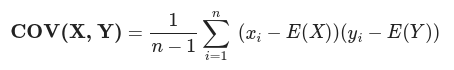
This explains how much X varies from its mean when Y varies from its own mean.
Covariance: How much does X vary from its mean when Y varies from its mean.
FÖnÜà1MXMià1FiÖn
average prediction
So saying "learning is slow" is really the same as saying that those partial derivatives are small.
given the same learning rate between 2 examples, as learning rate also affects the learning.
$$w = w - grad*lr$$
Monte Carlo Dropout boils down to training a neural network with the regular dropout and keeping it switched on at inference time. This way, we can generate multiple different predictions for each instance.
.
Long Short-Term Memory (LSTM) networks are a modified version of recurrent neural networks, which makes it easier to remember past data in memory. The vanishing gradient problem of RNN is resolved here.
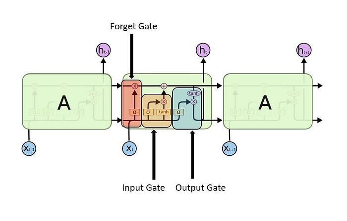
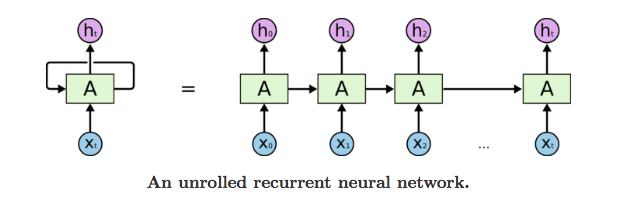
RNN is recurrent in nature as it performs the same function for every input of data while the output of the current input depends on the past one computation.
performs the same operation on every input of data,except it also previous outputs(called context) as another input.
Description:
First.it takes the X(0) from the sequence of input and then it outputs h(0) which together with X(1) is the input for the next step. So, the h(0) and X(1) is the input for the next step. Similarly, h(1) from the next is the input with X(2) for the next step and so on
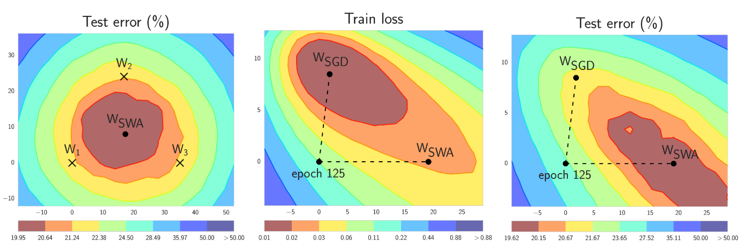
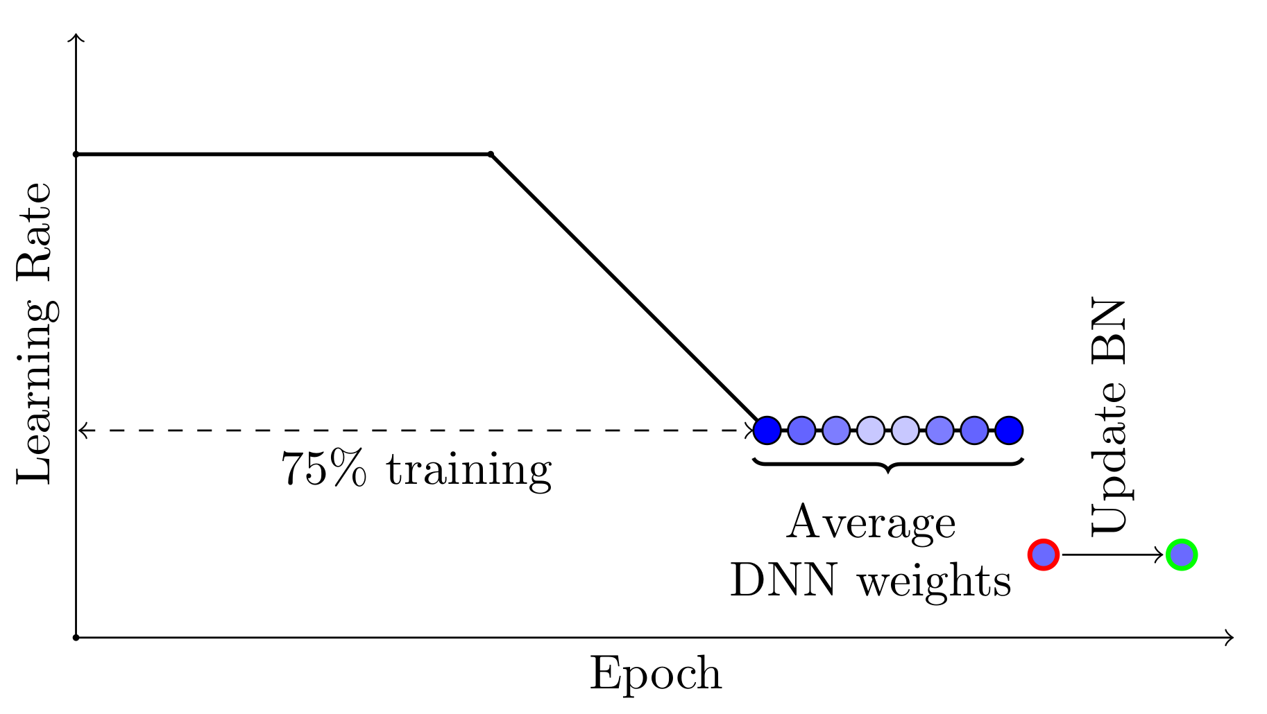
SWA uses a modified learning rate schedule so that SGD continues to explore the set of high-performing networks instead of simply converging to a single solution. For example, we can use the standard decaying learning rate strategy for the first 75% of training time, and then set the learning rate to a reasonably high constant value for the remaining 25% of the time (see the Figure 2 below). The second ingredient is to average the weights of the networks traversed by SGD. For example, we can maintain a running average of the weights obtained in the end of every epoch within the last 25% of training time (
Smaller batch sizes are used for two main reasons: Smaller batch sizes are noisy, offering a regularizing effect and lower generalization error. Smaller batch sizes make it easier to fit one batch worth of training data in memory (i.e. when using a GPU). A third reason is that the batch size is often set at something small, such as 32 examples, and is not tuned by the practitioner. Small batch sizes such as 32 do work well generally. … [batch size] is typically chosen between 1 and a few hundreds, e.g. [batch size] = 32 is a good default value — Practical recommendations for gradient-based training of deep architectures, 2012.
Training with a small batch size has a regularizing effect, and like most regularizers, can lead to very good generalization. In general, batch size 1 has the best generatlization:
Small batches can offer a regularizing effect (Wilson and Martinez, 2003), perhaps due to the noise they add to the learning process. Generalization error is often best for a batch size of 1. Training with such a small batch size might require a small learning rate to maintain stability because of the high variance in the estimate of the gradient. The total runtime can be very high as a result of the need to make more steps, both because of the reduced learning rate and because it takes more steps to observe the entire training set. (Deep Learning Book, p276)
The random noise from sampling mini-batches of data inSGD-like algorithms and random initialization of the deep neural networks, combined with the factthat there is a wide variety of local minima solutions in high dimensional optimization problem (Geet al., 2015; Kawaguchi, 2016; Wen et al., 2019), results in the following observation: deep neuralnetworks trained with different random seeds can converge to very different local minima althoughthey share similar error rates.
causes neural networks with the same architecture to converge to <mark>different local minima, but very similar error rates.</mark>.
On calling backward(), gradients are populated only for the nodes which have both requires_grad and is_leaf True. Gradients are of the output node from which .backward() is called, w.r.t other leaf nodes.
All layers declared inside of a neural network's __init__ method or as part of nn.Sequential automatically have their parameters set up with requires_grad=True and is_leaf=True. Autograd will therefore automatically store their gradients during a backward() call
However, it is well known that too large of a batch size will lead to poor generalization (although currently it’s not known why this is so).
the assumption in "Train longer, generalize better" is that it is due to making fewer updates: "we conducted experiments to show empirically that the "generalization gap" stems from the relatively small number of updates rather than the batch size, and can be completely eliminated by adapting" the training regime they use.
or equations (in LaTeX format)
Wrap your equation between 2$ on each side. $$Example$$.
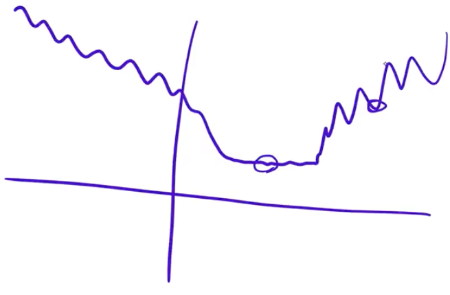
Loss functions usually have bumpy and flat areas (if you visualise them in 2D or 3D diagrams). Have a look at Fig. 3.2. If you end up in a bumpy area, that solution will tend not to generalise very well. This is because you found a solution that is good in one place, but it’s not very good in other place. But if you found a solution in a flat area, you probably will generalise well. And that’s because you found a solution that is not only good at one spot, but around it as well.
Another key point is that test distribution and train distribution are not always identical, therefore if you're in a flat area and test distribution shifts, you will still be in the flat area of the loss function but more around the edges. If you're in a sharp minima and distribution shifts, you're kicked out of it and end up somewhere higher up on the loss surface.
As mentioned earlier, I tested a lot of activation functions this year before Mish, and in most cases while things looked awesome in the paper, they would fall down as soon as I put them to use on more realistic datasets like ImageNette/Woof.Many of the papers show results using only MNIST or CIFAR-10, which really has minimal proof of how they will truly fare in my experience.
You should start with CIFAR-10 and MNIST only to get some initial results, but to see if those ideas hold up more broadly, test them on more realistic datasets like ImageWoof, ImageNet.
RAdam achieves this automatically by adding in a rectifier that dynamically tamps down the adaptive learning rate until the variance stabilizes.
RAdam reduces the variance of the adaptive learning rate early on Source
It is a good practice to first grid search through some orders of magnitude between 0.0 and 0.1, then once a level is found, to grid search on that level.
Once you can confirm that weight regularization may improve your overfit model, you can test different values of the regularization parameter.
Before using a hyperparmeter, first test that it will add value to your model. Only after that decide on value for it. If you don't want to use the default values, which you probably shouldn't given that hyperparameter values are very dependent on model architecture and dataset, then do something like grid search or randomized search through a model to find the best hyperparameter
An overfit model should show accuracy increasing on both train and test and at some point accuracy drops on the test dataset but continues to rise on the training dataset.
can also use loss: If training loss decreases while validation loss increases -> overfitting.
A weight regularizer can be added to each layer when the layer is defined in a Keras model.
i.e you can also set other hyperparameters(weight decay, learning rate, momentum, etc) per layer instead of whole network
add a penalty for weight size to the loss function.
l2 regularization can be done either by adding a penalty to the loss function and also directly to the weights through weight decay
SWA can be used with any learning rate schedule that encourages exploration of the flat region of solutions. For example, you can use cyclical learning rates in the last 25% of the training time instead of a constant value, and average the weights of the networks corresponding to the lowest values of the learning rate within each cycle (see Figure 3).
This is very similar to what a snapshot ensemble does, except that a snapshot ensemble doesn't average out the weights at the end. Instead, it uses each network it saved as part of an ensemble during inference.
The problem could be the optimizer’s old nemesis, pathological curvature. Pathological curvature is, simply put, regions of dt-math[block] { display: block; } fff which aren’t scaled properly. The landscapes are often described as valleys, trenches, canals and ravines. The iterates either jump between valleys, or approach the optimum in small, timid steps. Progress along certain directions grind to a halt. In these unfortunate regions, gradient descent fumbles.
Pathological curvature is a big problem for gradient descent and makes it significantly slow down: for a ravine, instead of going straight down through it, it oscillates sideways a lot since that's the direction where the gradient is larger, as it is immediately steeper:
